$\mathcal{R}^{2}$ curvature-squared corrections on Langevin diffusion coefficients

Abstract

The effect of finite coupling corrections to the Langevin diffusion coefficients on a moving heavy quark in the Super Yang-Mills plasma is investigated. These corrections are related to curvature squared corrections in the corresponding gravity sector. We compare the results of both longitudinal and perpendicular Langevin diffusion coefficients with those in $\mathcal{N}$=4 Super Yang-Mills plasma. It is observed that the curvature-squared corrections influence the Langevin diffusion coefficients, and the corrections for both Langevin diffusion coefficients demonstrate the dependence on the velocity of the moving heavy quark and the specifics of the higher derivative correction. In addition, we conduct calculations for the Langevin diffusion coefficients of a moving heavy quark within the Gauss-Bonnet background.

I Introduction

The heavy ion collisions experiments (HICs) at the Relativistic Heavy Ion Collider (RHIC) and the Large Hadron Collider (LHC) are believed to create almost the most perfect fluid Quark Gluon Plasma (QGP) Arsene et al. (2005); Adcox et al. (2005); Back et al. (2005); Adams et al. (2005). This provides a novel window for studying the physics of Quantum Chromodynamics (QCD) at strongly coupled regime. Since the properties of a strongly coupled system cannot be reliably calculated directly by perturbative techniques, one have to resort to some nonperturbative approaches to conquer the challenges.

AdS/CFT correspondence Maldacena (1998); Witten (1998a); Gubser et al. (1998) is one of the very promising approaches to deal with these problems in QCD at strong couple scenario where can’t be perturbatively handled properly Witten (1998b); Aharony et al. (2000). It is believed, on gravity sector, that an external quark on the gauge theory side is related to a string which has a single endpoint at the boundary and extends down to the horizon of an AdS black hole Gubser (2006); Herzog et al. (2006). Moreover, the diffusion of heavy quarks in a strongly coupled plasma can be understood as the fluctuation correlations of the trailing string. The studying of the stochastic nature of a heavy quark in a holography was proposed by Gubser (2008); Casalderrey-Solana and Teaney (2007). Soon the stochastic motion is formulated as a Langevin process de Boer et al. (2009); Son and Teaney (2009). Since the heavy quarks in HICs experiments are relativistic in many cases, the relativistic Langevin equation are studied in Giecold et al. (2009) and in non-conformal frameworks in Gursoy et al. (2010); Kiritsis et al. (2012) towards the multiple scales of QCD.

Methods in AdS/CFT relate a 4-dimensional $\mathcal{N}=4$ Super Yang-Mills (SYM) theory to a type-IIB string theory on the $AdS_{5}\times S^{5}$, and string theory contains higher derivative corrections to classical gravity from stringy $1/\lambda$ or quantum effects $1/N_{c}$ corrections. It’s natural to conduct computations for finite ’t Hooft coupling of gauge theory corresponding to studying the effect of higher derivative corrections on computations in classical Einstein gravity. The leading order corrections in $1/\lambda$ arises from stringy corrections to the low energy effective action of type-IIB supergravity $\alpha^{\prime 3}\mathcal{R}^{4}$ Pawelczyk and Theisen (1998), and apply such corrections to the ratio of shear viscosity over to entropy density of gauge field, $\eta/s$, was calculated in Benincasa and Buchel (2006); Buchel et al. (2005). Soon, it was found in Kats and Petrov (2009) that the universal low bound on the $\eta/s$ and causality can be violated when given a general $\mathcal{R}^{2}$ corrections to the gravitational action in GB gravity Brigante et al. (2008a); Kats and Petrov (2009); Brigante et al. (2008b); Buchel (2008); Neupane and Dadhich (2009); Neupane (2009); Ge et al. (2008). For instance the authors of Buchel (2008) studied the ratio of $\eta/s$ in 5 dimension setting, and the authors of Ge et al. (2008) studied the ratio in RN-AdS black branes solution finding that $\eta/s$ bound is violated and the Maxwell charge slightly reduces the deviation. For instance, the authors of Buchel (2008) studied the ratio of $\eta/s$ in a 5-dimensional setting, while Ge et al. (2008) discovered that the $\eta/s$ bound is violated and the presence of Maxwell charge slightly reduces the deviation in the RN-AdS black brane solution. Motivated by these vast string landscapes, the effect of high derivative curvature $\mathcal{R}^{4}$ or $\mathcal{R}^{2}$ corrections on the different aspects properties of QGP has been studied in Ali-Akbari and Bitaghsir Fadafan (2010); Ali-Akbari and Fadafan (2011); Zhang et al. (2023); Arnold et al. (2012); Atashi and Bitaghsir Fadafan (2020); Li et al. (2018); Zhang et al. (2018). Besides, the authors of Myers and Robinson (2010); Oliva and Ray (2010a, b); Zhu et al. (2024) studied curvature-cubic $\mathcal{R}^{3}$ corrections to $\mathrm{AdS_{5}}$.

One of the significant applications of the AdS/CFT correspondence is the investigation of jet quenching phenomena involving high transverse momentum partons produced in HICs. It is found in Ficnar et al. (2014) that introducing $\mathcal{R}^{2}$ corrections to the $\mathrm{AdS_{5}}$ yields a substantial increase in nuclear modification factor $R_{AA}$. The initial $1/\lambda$ correction to the jet quenching parameter was found in Armesto et al. (2006), followed by the jet quenching parameter include $\mathcal{R}^{2}$ correction Zhang et al. (2016); Bitaghsir Fadafan (2010). The trailing string, which models the drag force on a moving heavy quark, has been examined within the framework of higher derivative gravity to investigate the $\mathcal{R}^{2}$ and $\mathcal{R}^{4}$ correction to drag force in Vazquez-Poritz (2008); Fadafan (2008). In this study, we focus on investigating $\mathcal{R}^{2}$ corrections to Langevin diffusion coefficients (LGV-coefficients) that are related to the fluctuations of the trailing string.

The organization of this paper is as follows. In the subsequent section, section II, we will review the main procedures to deduce LGV-coefficients within the membrane paradigm. Additionally, we also discuss numerical results of $\mathcal{R}^{2}$ correction to LGV-Coefficients in section II. In section III, we will study $\mathcal{R}^{2}$ correction with GB gravity to LGV-coefficients as in section II. The last part section IV is devoted to conclusions and discussion.

II Curvature squared corrections to AdS-Schwarzschild black brane

The curvature squared corrections to solution of $AdS_{5}$-Schwarzschild black brane can be described by the general action Brigante et al. (2008b, a)

$$\begin{split}S=\frac{1}{16\pi G_{5}}&\int d^{5}\sqrt{-g}\times\left[\mathcal{R}-\Lambda+L^{2}\left(c_{1}\mathcal{R}^{2}+c_{2}\mathcal{R}_{\mu\nu}\mathcal{R}^{\mu\nu}+c_{3}\mathcal{R}_{\mu\nu\rho\sigma}\mathcal{R}^{\mu\nu\rho\sigma}\right)\right]\end{split}$$ (1)

where $G_{5}=\pi L^{3}/2N_{c}^{2}$ is 5-dimensional Newton constant, $\mathcal{R}$ is the Ricci scalar, $\mathcal{R}_{\mu\nu}$ and $\mathcal{R}_{\mu\nu\rho\sigma}$ are the Ricci tensor and Riemann tensor, respectively. The negative cosmological constant $\Lambda=-\frac{12}{L^{2}}$ creates an $AdS$ space with the radius $L$. The parameter $c_{i}$ are are expected to be of $o(\alpha^{\prime})$ which means $c_{i}=0$ in the limit of large ’t Hooft coupling. At this order, $c_{3}$ is unambiguous while $c_{1}$ and $c_{2}$ can be arbitrarily varied by a metric redefinition Kats and Petrov (2009); Noronha and Dumitru (2009).

The black brane solution of $AdS_{5}$ space for (1) is given by Kats and Petrov (2009),

$$ds^{2}=-(\frac{r^{2}}{L^{2}})f(r)dt^{2}+(\frac{r^{2}}{L^{2}})d\vec{x}^{2}+\frac{L^{2}}{r^{2}f(r)}dr^{2},$$ (2)

where

$$f(r)=1-\frac{r_{h}^{4}}{r^{4}}+\alpha+\beta\frac{r_{h}^{8}}{r^{8}}$$ (3)

and

$$\alpha=\frac{2}{3}\left(10c_{1}+2c_{2}+c_{3}\right),\,\,\,\beta=2c_{3}.$$ (4)

The boundary of the asymptotically AdS geometry is located at $r\rightarrow\infty$ where $r$ denotes the 5th dimensional radial coordinate, and $(t,\vec{x})$ label the left 4-dimensional spacetime of gauge theory on boundary. One can solve $f(r)=0$ to find location of the horizon $r=r_{h}$.

The heat bath temperature is given by

$$T_{R^{2}}=\frac{r_{h}}{\pi L^{2}}\left(1+\frac{1}{4}\alpha-\frac{5}{4}\beta\right).$$ (5)

By following the authors of Gursoy et al. (2010); Giataganas and Soltanpanahi (2014); Finazzo et al. (2016), we compute the LGV-coefficients of a heavy quark in squared-curvature correction background. It more conveniences to conduct the calculation in a more general form,

$$ds^{2}=g_{tt}dt^{2}+g_{x_{p}x_{p}}dx^{2}+g_{rr}dr^{2}.$$ (6)

From (2), one has the

$$g_{tt}=-(\frac{r^{2}}{L^{2}})f(r),\quad g_{x_{p}x_{p}}=\frac{r^{2}}{L^{2}},\quad g_{rr}=\frac{L^{2}}{r^{2}f(r)}.$$ (7)

Holographically, the moving heavy quark of infinite mass on the boundary CFT correspond to the endpoint of the trailing string. The string dynamics are captured by the Nambu-Goto action

$$\begin{split}S_{NG}=-\frac{1}{2\pi\alpha^{\prime}}\int\mathrm{d}\sigma^{\alpha}\mathrm{d}\sigma^{\beta}\sqrt{-\mathrm{det}g_{\alpha\beta}},\qquad g_{\alpha\beta}=g_{\mu\nu}\frac{\partial X^{\mu}}{\partial\sigma^{\alpha}}\frac{\partial X^{\nu}}{\partial\sigma^{\beta}}.\end{split}$$ (8)

where $g_{\alpha\beta}$ is the induced metric, and $g_{\mu\nu}$ and $X_{\mu}$ are the branes metric and target space coordinates.

Given a moving heavy quark with a constant velocity $v$, one can choose to compute in static gauge for the string world-sheet and has the usual parametrization

$$t=\sigma^{\alpha},\quad r=\sigma^{\beta},\quad x=vt+\xi(r),$$ (9)

where $\xi$ is the profile of the string in the bulk. It’s is deduced the world-sheet metric

$$g_{\alpha\beta}=\left(\begin{matrix}g_{tt}+v^{2}g_{pp}&g_{pp}v\xi^{\prime}\\ g_{pp}v\xi^{\prime}&g_{rr}+g_{pp}\xi^{{}^{\prime}2}\end{matrix}\right),$$ (10)

and the corresponding action

$$S_{NG}=-\frac{1}{2\pi\alpha^{\prime}}\int\mathrm{d}t\mathrm{d}r\sqrt{-(g_{tt}g_{rr}+g_{tt}g_{pp}\xi^{\prime 2}+g_{pp}g_{rr}v^{2})}.$$ (11)

It’s obvious that radial conjugate momentum $\pi_{\xi}$ is conserved for the simple motion

$$\begin{split}\pi_{\xi}=\frac{\delta S}{\delta\xi}=-\frac{1}{2\pi\alpha^{\prime}}\frac{g_{tt}g_{pp}\xi^{\prime}}{2\sqrt{-(g_{tt}g_{rr}+g_{tt}g_{pp}\xi^{\prime 2}+g_{pp}g_{rr}v^{2})}}.\end{split}$$ (12)

It is easy to find $\xi^{\prime}$ from (12) as

$$\xi^{\prime}=\sqrt{\frac{-g_{tt}g_{rr}-g_{pp}g_{rr}v^{2}}{g_{tt}g_{xx}(1+\frac{g_{tt}g_{xx}}{C^{2}})}},$$ (13)

where $C\equiv 2\pi\alpha^{\prime}\pi_{\xi}$. The world-sheet of the string has a horizon and turns out to be the same with critical point $r_{c}$ at which both numerator and denominator change their sign. By inserting (7) into $g_{\alpha\alpha}(r_{c})=0$, one can identify the critical point $r_{c}$ as

$$r_{c}=\sqrt[4]{\frac{r_{h}^{4}\sqrt{1-4\beta\left(\alpha-v^{2}+1\right)}+r_{h}^{4}}{2\left(\alpha-v^{2}+1\right)}}.$$ (14)

One can also find the effective temperature $T_{ws}$ of the world-sheet horizon by diagonal world-sheet metric (10). One can change coordinates to diagonalize the induced metric, by means of the reparametrization,

$$d\sigma^{\alpha}\rightarrow d\sigma^{\alpha}+\frac{g_{\alpha\beta}}{g_{\alpha\alpha}}d\sigma^{\beta}.$$ (15)

The diagonal induced world-sheet metric $h_{\alpha\beta}$ given

$$h_{\alpha\beta}=\left(\begin{matrix}g_{tt}+g_{pp}v^{2}&\\ &\frac{g_{tt}g_{pp}g_{rr}}{g_{tt}g_{pp}+v^{2}g_{pp}|_{r=r_{c}}}\end{matrix}\right).$$ (16)

Following the usual procedure, the effective world sheet temperature reads

$$T^{2}_{ws} =\frac{1}{16\pi^{2}}\left(h_{\alpha\alpha}^{\prime}\,\left(h^{\beta\beta}\right)^{\prime}\right)\bigg{|}_{r_{c}}$$ (17)

$$=\frac{1}{16\pi^{2}}\left[(g_{tt}+v^{2}g_{pp})^{\prime}(\frac{g_{tt}g_{pp}+v^{2}(g_{pp}|_{r_{c}})^{2}}{g_{tt}g_{pp}g_{uu}})^{\prime}\right]^{2}\bigg{|}_{r=r_{c}}$$

$$=\frac{1}{16\pi^{2}}\absolutevalue{\frac{g^{{}^{\prime}2}_{tt}-v^{4}g^{{}^{\prime}2}_{pp}}{g_{tt}g_{pp}}}\bigg{|}_{r=r_{c}}$$

$$=\frac{1}{16\pi^{2}}\absolutevalue{\frac{1}{g_{tt}g_{rr}}(g_{tt}g_{pp})^{\prime}(\frac{g_{tt}}{g_{pp}})^{\prime}}\bigg{|}_{r=r_{c}}.$$

By inserting (14) into (17), one have the effective temperature $T^{ws}_{R^{2}}$ in

$$T^{ws}_{R^{2}}=\frac{1}{4\pi}\absolutevalue{\sqrt{\left(\frac{8\beta r_{h}^{8}}{r_{c}^{9}}-\frac{4r_{h}^{4}}{r_{c}^{5}}\right)\left(4r_{c}^{3}\left(\alpha+\frac{\beta r_{h}^{8}}{r_{c}^{8}}-\frac{r_{h}^{4}}{r_{c}^{4}}+1\right)+r_{c}^{4}\left(\frac{4r_{h}^{4}}{r_{c}^{5}}-\frac{8\beta r_{h}^{8}}{r_{c}^{9}}\right)\right)}}.$$ (18)

In the conformal limit, where $\alpha\rightarrow 0,\,\beta\rightarrow 0$, the background solution reduces to AdS-BH, the world-sheet temperature (18) is simply

$$T_{R^{2}}=\gamma\lim_{\alpha\rightarrow 0,\beta\rightarrow 0}T^{ws}_{R2},$$ (19)

where $\gamma$ is the Lorentz factor $\gamma=1/\sqrt{1-v^{2}}$.

Considering the fluctuation in classical trailing string, one has

$$t=\sigma^{\alpha},r=\sigma^{\beta},x_{p}=vt+\xi(r)+\delta x_{p}(\sigma^{\alpha},\sigma^{\beta}),$$ (20)

where the fluctuation of the form $\delta x_{p}(\sigma^{\alpha},\sigma^{\beta})$ along longitudinal and transverse direction of $x_{p}|_{(1,2,3)}$. A simple expression for the quadratic action in the worldsheet embedding fluctuations capturing fluctuations of heavy quark reads

$$\begin{split}S_{quadratic}=-\frac{1}{2\pi\alpha^{\prime}}\int d\tau dr\frac{H^{\alpha\beta}}{2}\times(N[r]\partial_{\alpha}\delta x_{p}\partial_{\beta}\delta x_{p}+\sum_{i\neq p}g_{ii}\partial_{\alpha}\delta x_{i}\partial_{\beta}\delta x_{i}),\\ N(r)\equiv\frac{g_{tt}g_{pp}+C^{2}}{g_{tt}+g_{pp}v^{2}},\\ H^{\alpha\beta}=\sqrt{-det(h)}h^{\alpha\beta},\\ \end{split}$$ (21)

where $h^{\alpha\beta}$ is inverse of the diagonalized induced world-sheet metric. We recommend referring to Gubser (2008); Gursoy et al. (2010); Giataganas and Soltanpanahi (2014); Chakrabortty et al. (2014) for a detailed proof. For an arbitrary massless fluctuation $\phi$ with an action

$$S_{example}=-1/2\int dxdr\sqrt{-g}Q(r)g^{\alpha\beta}\partial_{\alpha}\partial_{\beta}\phi.$$ (22)

Taking advantage of the membrane paradigm Iqbal and Liu (2009), one can directly reads the transport coefficient associated with the retarded Green’s function form (22) without solving motion equation as

$$\begin{split}\chi_{R}&=-\lim_{k_{\mu}\rightarrow 0}\frac{\imaginary G_{R}(\vec{k},\omega)}{\omega}=Q(r_{h})\end{split}$$ (23)

where $Q$ is the effective coupling of the fluctuation and the metric dependence drops out in 2-dimension.

The LGV-coefficient is defined in terms of the symmetric correlator as

$$\begin{split}\kappa_{a}&=\lim_{\omega\rightarrow 0}G^{a}_{sym}(\omega)\\ &=-\coth{\frac{\omega}{2T_{ws}}}\lim_{\omega\rightarrow 0}(\imaginary G^{a}_{R}(\omega))\\ &=-2T_{ws}\lim_{\omega\rightarrow 0}\frac{\imaginary G^{a}_{R}(\omega)}{\omega}\\ &=2T_{ws}\chi_{R}^{a}\\ &=2T_{ws}Q^{a}(r_{c}).\end{split}$$ (24)

where $a=(\perp,\parallel)$. The second step has employed the $\omega\rightarrow 0$ limit of $G^{a}_{sym}(\omega)=\coth{\frac{\omega}{2T}}\imaginary G^{a}_{R}(\omega)$, and the third step has employed (23). By comparison of (21) and (22) yields,

$$Q^{\perp}=\frac{1}{2\pi\alpha}g_{kk}\bigg{|}_{r=r_{c}},\qquad Q^{\parallel}=\frac{1}{2\pi\alpha}\lim_{r\rightarrow r_{c}}N(r)=\frac{1}{2\pi\alpha}\frac{(g_{tt}g_{pp})^{\prime}}{g_{pp}(\frac{g_{tt}}{g_{pp}})^{\prime}}\bigg{|}_{r=r_{c}}.$$ (25)

Noticing $N(r_{c})=\frac{0}{0}$, therefore, one needs to use the L’Hopital’s rule to calculate the limit. One can also insert (25) into (24) and yields,

$$\kappa_{\perp}=\frac{1}{\pi\alpha^{\prime}}g_{kk}|_{r=r_{c}}T_{ws},\qquad\kappa_{\parallel}=\frac{1}{\pi\alpha^{\prime}}\frac{(g_{tt}g_{pp})^{\prime}}{g_{pp}(\frac{g_{tt}}{g_{pp}})^{\prime}}\bigg{|}_{r=r_{c}}T_{ws}.$$ (26)

In our case, one can also insert metric (7) into (26) and yields,

$$\kappa_{\perp}=\frac{\sqrt{\lambda}}{\pi}r_{c}^{2}T^{ws}_{R2},$$ (27)

and

$$\kappa_{\parallel}=\frac{-4r_{c}^{3}\sqrt{\lambda}\left(\alpha+\frac{\beta r_{h}^{8}}{r_{c}^{8}}-\frac{r_{h}^{4}}{r_{c}^{4}}+1\right)-r_{c}^{4}\left(\frac{4r_{h}^{4}}{r_{c}^{5}}-\frac{8\beta r_{h}^{8}}{r_{c}^{9}}\right)}{\pi r_{c}^{2}\left(\frac{8\beta r_{h}^{8}}{r_{c}^{9}}-\frac{4r_{h}^{4}}{r_{c}^{5}}\right)}T^{ws}_{R2}.$$ (28)

In conformal limit, one can obtain the well-known results Gubser (2008); Casalderrey-Solana and Teaney (2007)

$$\begin{split}\kappa_{\perp}^{SYM}=\sqrt{\lambda}\pi T^{3}\gamma^{\frac{1}{2}},\qquad\kappa_{\parallel}^{SYM}=\sqrt{\lambda}\pi T^{3}\gamma^{\frac{5}{2}}.\end{split}$$ (29)

One can check that (27) and (28) reduce to this results by taking the limit of $\alpha\rightarrow 0$ and $\beta\rightarrow 0$.

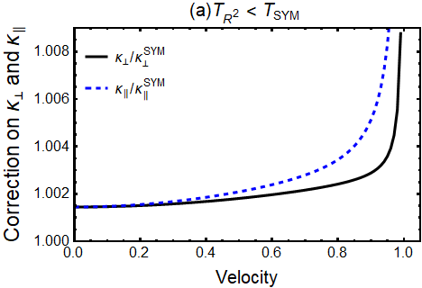
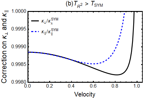
Figure 1: The correction to transverse LGV-coefficients $\kappa_{\perp}$ and longitudinal LGV-coefficients $\kappa_{\parallel}$ as a function of velocity of the heavy quark, normalized by the conformal limit respectively.

The effects from $\mathcal{R}^{2}$ corrections to the classical trailing string, which models the drag force on a moving heavy quark in SYM plasma, were studied by the authors of Fadafan (2008) at two distinct scenarios: $T_{R^{2}}<T_{SYM}$ and $T_{R^{2}}>T_{SYM}$. Following their convention, we find it is convenient to explore the curvature squared corrections on the fluctuations of the trailing string that is related to LGV-coefficients. More precisely, we investigate the $\mathcal{R}^{2}$ corrections to $\kappa_{\perp}$ and $\kappa_{\parallel}$ by evaluating (27) and (28) using two distinct sets of values for the parameters $\alpha$ and $\beta$.

Fig.1 demonstrates the impact of $\mathcal{R}^{2}$ corrections on LGV-coefficients where $\kappa_{\perp}$ and $\kappa_{\parallel}$ normalized by the SYM result at zero baryon density given in (29). Plots (a) in Fig.1 show $\mathcal{R}^{2}$ corrections on LGV-coefficients at fixed small values of $\alpha=-0.0005$ and $\beta=+0.0006$ corresponding to $T_{R^{2}}<T_{SYM}$. It is clear from this plot that the $\mathcal{R}^{2}$ corrections to the both $\kappa_{\perp}$ and $\kappa_{\parallel}$ are increased monotonically with increasing the moving velocity of the heavy quark and the corrections to the LGV-coefficient are larger than SYM case at all velocities.

However, it is also observed that this kind of $\mathcal{R}^{2}$ correction can also be smaller than $\mathcal{N}=4$ SYM results in Plots (b) in Fig.1 at $\alpha=-0.0005$ and $\beta=-0.0007$ corresponding to $T_{R^{2}}>T_{SYM}$. In this case, a critical velocity ($v_{c}$) exists where the corrections increase both $\kappa_{\perp}$ and $\kappa_{\parallel}$ if $v>v_{c}$ while corrections decrease both $\kappa_{\perp}$ and $\kappa_{\parallel}$ if $v>v_{c}$.

As a result, we conclude that the finite coupling corrections affect the both $\kappa_{\perp}$ and $\kappa_{\parallel}$ on a moving quark in the strongly-coupled plasma and depend on the details of curvature squared corrections. The LGV-coefficient can be larger than or smaller than that in the infinite-coupling case. But at a fixed velocity, one can always find that the corrected $\kappa_{\parallel}$ is at least as large as corrected $\kappa_{\perp}$. Moreover, the universal relation, $\kappa_{L}\geq\kappa_{T}$ which founded by the authors of Gursoy et al. (2010), always hold both when $T_{R^{2}}>T_{SYM}$ and $T_{R^{2}}<T_{SYM}$. Our findings are similar to the case of drag force on a moving heavy quark in Fadafan (2008).

III Gauss-Bonnet gravity as special case of curvature squared correction

The Gauss-Bonnet (GB) gravity Zwiebach (1985) is one of the most general theory of gravity with curvature squared correction in five dimensions. The exact solutions and thermodynamic properties of the GB background were discussed in Cai (2002); Nojiri and Odintsov (2001, 2002). One can also consider the GB gravity as a special case of the general action (1) where $c_{2}=-4c_{1}$ and $c_{1}=c_{3}=\lambda_{GB}/2$. This yields the action defined as,

$$\begin{split}S=&\frac{1}{16\pi G_{5}}\int d^{5}x\sqrt{-g}\times\Bigg{[}\mathcal{R}-\Lambda+L^{2}\frac{\lambda_{GB}}{2}\left(\mathcal{R}^{2}-4\mathcal{R}_{\mu\nu}\mathcal{R}^{\mu\nu}+\mathcal{R}_{\mu\nu\rho\sigma}\mathcal{R}^{\mu\nu\rho\sigma}\right)\Bigg{]}.\end{split}$$ (30)

The dimensionless Gauss-Bonnet coupling constant $\lambda_{GB}$ can be constrained by causality Brigante et al. (2008a) and the positive boundary energy density on the boundary Hofman and Maldacena (2008) to be:

$$-\frac{7}{36}<\lambda_{GB}\leq\frac{9}{100}.$$ (31)

A black hole solution in this case is known analytically Cai (2002):

$$ds^{2}=-a\frac{r^{2}}{L^{2}}f_{GB}(r)dt^{2}+\frac{r^{2}}{L^{2}}d\vec{x}^{2}+\frac{L^{2}}{r^{2}f_{GB}(r)}dr^{2},$$ (32)

where

$$\begin{split}f_{GB}(r)&=\frac{1}{2\lambda_{GB}}\left(1-\sqrt{1-4\lambda_{GB}(1-r_{h}^{4}/r^{4})}\right)\,,\\ a&=\frac{1}{2}\left(1+\sqrt{1-4\lambda_{GB}}\right)\,.\end{split}$$ (33)

The boundary of the metric (32) is at $r\rightarrow\infty$. We choose the parameter $a$ to specify the speed of light of the boundary gauge theory be unity. As a result, one can easily find

$$f_{GB}(r\xrightarrow{}\infty)=\frac{1}{a}.$$ (34)

The heat bath temperature of the black hole is given by

$$T_{GB}=\frac{\sqrt{a}r_{h}}{\pi L^{2}},$$ (35)

where the horizon position $r_{h}$ depends on $\lambda_{GB}$ in a fixed $T_{GB}$.

Using a general form of metric, one has

$$\begin{split}g_{tt}(r)=-a\frac{r^{2}}{L^{2}}f_{GB}(r),\qquad g_{xx}(r)=\frac{r^{2}}{L^{2}},\qquad g_{rr}(r)=\frac{L^{2}}{r^{2}f_{GB}(r)}.\end{split}$$ (36)

In our analysis, we set $AdS_{5}$-radius to be unity for convenience. Using the same procedures as before, we can easily find the critical value $r^{c}_{GB}$ where the numerator and denominator change sign at the same value,

$$r^{c}_{GB}=\frac{\sqrt{a}(r_{h})}{\left(a(a-v^{2})+\lambda_{GB}v^{4}\right)^{\frac{1}{4}}}.$$ (37)

The world-sheet temperature of GB gravity of a quark feel is denoted as $T^{ws}_{GB}$,

$$T^{ws}_{GB}=\frac{1}{4\pi}\left(\absolutevalue{\frac{4(r_{h})^{4}\left(-\frac{2a(1-K_{10})(r^{c}_{GB})^{3}}{\lambda_{GB}}-\frac{4a(r_{h})^{4}}{K_{10}r^{c}_{GB}}\right)}{K_{10}(r^{c}_{GB})^{5}}}\right)^{\frac{1}{2}},\qquad K_{10}=\sqrt{1-4\lambda_{GB}\left(1-\frac{(r_{h})^{4}}{(r^{c}_{GB})^{4}}\right)}.$$ (38)

Asserting (36) to (17), (28) and (27), one get longitudinal and perpendicular LGV-coefficients as

$$\begin{split}\kappa^{\perp}_{GB}&=\frac{\sqrt{\lambda}}{\pi}(r^{c}_{GB})^{2}T^{ws}_{GB}\end{split}$$ (39)

and

$$\begin{split}\kappa^{\parallel}_{GB}&=-\frac{\sqrt{\lambda}K_{10}(r^{c}_{GB})^{3}\left(-\frac{2a(1-K_{10})(r^{c}_{GB})^{3}}{\lambda_{GB}}-\frac{4a(r_{h})^{4}}{K_{10}r^{c}_{GB}}\right)}{4\pi a(r_{h})^{4}}T^{ws}_{GB}.\end{split}$$ (40)

One can check that (39) and (40) reduce to the results in conformal limit (29) by taking the limit of $\lambda_{GB}\rightarrow 0$.

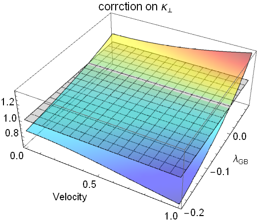
Figure 2: The corrections to the transverse LGV-coefficients $\kappa_{\perp}$ (left panel) and the longitudinal LGV-coefficients $\kappa_{\parallel}$ (right panel) are shown as functions of both velocity and $\lambda_{GB}$, respectively normalized by the conformal limit.

By employing GB gravity, we now discuss the $\mathcal{R}^{2}$ corrections on the LGV-coefficients, normalized by the limits given in (29) for $\mathcal{N}=4$ SYM. Plots (a) and (b) in Figure 2 depict $\kappa_{\perp}$ and $\kappa_{\parallel}$ respectively as functions of moving velocity and $\lambda_{GB}$. It is evident that both the $\kappa_{\perp}$ and $\kappa_{\parallel}$ are independent on the values of moving velocity and $\lambda_{GB}$. It’s also find that the correction behaviors to $\kappa_{\perp}$ and $\kappa_{\parallel}$ are notably similar, and the universal relation $\kappa_{\parallel}\geq\kappa_{\perp}$ identified by the authors of Gursoy et al. (2010) also holds in the context of GB gravity.

It is found that the results of LGV-coefficients in the GB gravity, when $\lambda_{GB}=0$, will reduce to the case corresponding to $\mathcal{N}=4$ SYM. For $\lambda_{GB}>0$, Fig.2 demonstrates that the corrections to the $\kappa_{\perp}$ and $\kappa_{\parallel}$ become stronger monotonically with increasing velocity of the moving heavy quark or with the increasing $\lambda_{GB}$. Conversely, for $\lambda_{GB}<0$, the $\kappa_{\perp}$ and $\kappa_{\parallel}$ for a moving heavy quark under GB gravity will be less than those in the $\mathcal{N}=4$ SYM case. Furthermore, the corrections to the $\kappa_{\perp}$ and $\kappa_{\parallel}$ increase monotonically with the increasing the absolute value of $\lambda_{GB}$, and also increase with the growing velocity of the moving heavy quark.

IV Summary

Using classical gravity to understand a quantum system is one of the most profound discoveries of contemporary theoretical physics. The majority of computations, achieved through classical two-derivative gravity calculations, hold strict validity within the context of a large ’t Hooft coupling $\lambda$ and the limit of color number $N_{c}$. The modification of quenched jets provide one of the most effective tools for constraining properties of the QGP produced in heavy ion collisions. In this study, we take an investigation on finite coupling corrections to heavy quark diffusion.

We have examined the influences from curvature-squared $\mathcal{R}^{2}$ corrections on the AdS black brane metric to LGV-coefficients with both a more general $\mathcal{R}^{2}$ gravity and the GB gravity. Our investigation reveals that finite coupling corrections can indeed impact the $\kappa_{\perp}$ and $\kappa_{\parallel}$ values of a moving heavy quark. However, the specific correction behaviors depend on the details of higher derivative gravity. Both the $\kappa_{L}$ and $\kappa_{T}$ can be larger than or smaller than that in the infinite coupling case. Both $\kappa_{L}$ and $\kappa_{T}$ values can either increase or decrease in comparison to the infinite coupling scenario. We confirm the persistence of the universal relation $\kappa_{L}\geq\kappa_{T}$ across all cases we examined. Our findings regarding curvature squared corrections to $\kappa_{L}$ and $\kappa_{T}$ closely resemble the features obtained for the drag force on a moving heavy quark discussed in Fadafan (2008). Finally, we should emphasize that we do not predict the effects of finite ’t Hooft correction to $\mathcal{N}=4$ SYM, since the leading correction in gauge theory enters at order $R^{4}$.

References

- Arsene et al. (2005) I. Arsene et al. (BRAHMS), Nucl. Phys. A 757, 1 (2005), arXiv:nucl-ex/0410020 .
- Adcox et al. (2005) K. Adcox et al. (PHENIX), Nucl. Phys. A 757, 184 (2005), arXiv:nucl-ex/0410003 .
- Back et al. (2005) B. B. Back et al. (PHOBOS), Nucl. Phys. A 757, 28 (2005), arXiv:nucl-ex/0410022 .
- Adams et al. (2005) J. Adams et al. (STAR), Nucl. Phys. A 757, 102 (2005), arXiv:nucl-ex/0501009 .
- Maldacena (1998) J. M. Maldacena, Adv. Theor. Math. Phys. 2, 231 (1998), arXiv:hep-th/9711200 .
- Witten (1998a) E. Witten, Adv. Theor. Math. Phys. 2, 253 (1998a), arXiv:hep-th/9802150 .
- Gubser et al. (1998) S. S. Gubser, I. R. Klebanov, and A. M. Polyakov, Phys. Lett. B 428, 105 (1998), arXiv:hep-th/9802109 .
- Witten (1998b) E. Witten, Adv. Theor. Math. Phys. 2, 505 (1998b), arXiv:hep-th/9803131 .
- Aharony et al. (2000) O. Aharony, S. S. Gubser, J. M. Maldacena, H. Ooguri, and Y. Oz, Phys. Rept. 323, 183 (2000), arXiv:hep-th/9905111 .
- Gubser (2006) S. S. Gubser, Phys. Rev. D 74, 126005 (2006), arXiv:hep-th/0605182 .
- Herzog et al. (2006) C. P. Herzog, A. Karch, P. Kovtun, C. Kozcaz, and L. G. Yaffe, JHEP 07, 013 (2006), arXiv:hep-th/0605158 .
- Gubser (2008) S. S. Gubser, Nucl. Phys. B 790, 175 (2008), arXiv:hep-th/0612143 .
- Casalderrey-Solana and Teaney (2007) J. Casalderrey-Solana and D. Teaney, JHEP 04, 039 (2007), arXiv:hep-th/0701123 .
- de Boer et al. (2009) J. de Boer, V. E. Hubeny, M. Rangamani, and M. Shigemori, JHEP 07, 094 (2009), arXiv:0812.5112 [hep-th] .
- Son and Teaney (2009) D. T. Son and D. Teaney, JHEP 07, 021 (2009), arXiv:0901.2338 [hep-th] .
- Giecold et al. (2009) G. C. Giecold, E. Iancu, and A. H. Mueller, JHEP 07, 033 (2009), arXiv:0903.1840 [hep-th] .
- Gursoy et al. (2010) U. Gursoy, E. Kiritsis, L. Mazzanti, and F. Nitti, JHEP 12, 088 (2010), arXiv:1006.3261 [hep-th] .
- Kiritsis et al. (2012) E. Kiritsis, L. Mazzanti, and F. Nitti, J. Phys. G 39, 054003 (2012), arXiv:1111.1008 [hep-th] .
- Pawelczyk and Theisen (1998) J. Pawelczyk and S. Theisen, JHEP 09, 010 (1998), arXiv:hep-th/9808126 .
- Benincasa and Buchel (2006) P. Benincasa and A. Buchel, JHEP 01, 103 (2006), arXiv:hep-th/0510041 .
- Buchel et al. (2005) A. Buchel, J. T. Liu, and A. O. Starinets, Nucl. Phys. B 707, 56 (2005), arXiv:hep-th/0406264 .
- Kats and Petrov (2009) Y. Kats and P. Petrov, JHEP 01, 044 (2009), arXiv:0712.0743 [hep-th] .
- Brigante et al. (2008a) M. Brigante, H. Liu, R. C. Myers, S. Shenker, and S. Yaida, Phys. Rev. D 77, 126006 (2008a), arXiv:0712.0805 [hep-th] .
- Brigante et al. (2008b) M. Brigante, H. Liu, R. C. Myers, S. Shenker, and S. Yaida, Phys. Rev. Lett. 100, 191601 (2008b), arXiv:0802.3318 [hep-th] .
- Buchel (2008) A. Buchel, Phys. Lett. B 665, 298 (2008), arXiv:0804.3161 [hep-th] .
- Neupane and Dadhich (2009) I. P. Neupane and N. Dadhich, Class. Quant. Grav. 26, 015013 (2009), arXiv:0808.1919 [hep-th] .
- Neupane (2009) I. P. Neupane, Int. J. Mod. Phys. A 24, 3584 (2009), arXiv:0904.4805 [gr-qc] .
- Ge et al. (2008) X.-H. Ge, Y. Matsuo, F.-W. Shu, S.-J. Sin, and T. Tsukioka, JHEP 10, 009 (2008), arXiv:0808.2354 [hep-th] .
- Ali-Akbari and Bitaghsir Fadafan (2010) M. Ali-Akbari and K. Bitaghsir Fadafan, Nucl. Phys. B 835, 221 (2010), arXiv:0908.3921 [hep-th] .
- Ali-Akbari and Fadafan (2011) M. Ali-Akbari and K. B. Fadafan, Nucl. Phys. B 844, 397 (2011), arXiv:1008.2430 [hep-th] .
- Zhang et al. (2023) Z.-q. Zhang, X. Zhu, and D.-f. Hou, Eur. Phys. J. C 83, 389 (2023).
- Arnold et al. (2012) P. Arnold, P. Szepietowski, and D. Vaman, JHEP 07, 024 (2012), arXiv:1203.6658 [hep-th] .
- Atashi and Bitaghsir Fadafan (2020) M. Atashi and K. Bitaghsir Fadafan, Phys. Lett. B 800, 135090 (2020), arXiv:1906.11621 [hep-th] .
- Li et al. (2018) F. Li, Z.-Q. Zhang, and G. Chen, Chin. Phys. C 42, 123109 (2018), arXiv:1809.10898 [hep-th] .
- Zhang et al. (2018) Z.-q. Zhang, Z.-j. Luo, and D.-f. Hou, Annals Phys. 391, 47 (2018), arXiv:1803.00775 [hep-th] .
- Myers and Robinson (2010) R. C. Myers and B. Robinson, JHEP 08, 067 (2010), arXiv:1003.5357 [gr-qc] .
- Oliva and Ray (2010a) J. Oliva and S. Ray, Class. Quant. Grav. 27, 225002 (2010a), arXiv:1003.4773 [gr-qc] .
- Oliva and Ray (2010b) J. Oliva and S. Ray, Phys. Rev. D 82, 124030 (2010b), arXiv:1004.0737 [gr-qc] .
- Zhu et al. (2024) Z.-R. Zhu, M. Sun, R. Zhou, and J. Han, (2024), arXiv:2401.05893 [hep-ph] .
- Ficnar et al. (2014) A. Ficnar, S. S. Gubser, and M. Gyulassy, Phys. Lett. B 738, 464 (2014), arXiv:1311.6160 [hep-ph] .
- Armesto et al. (2006) N. Armesto, J. D. Edelstein, and J. Mas, JHEP 09, 039 (2006), arXiv:hep-ph/0606245 .
- Zhang et al. (2016) Z.-q. Zhang, D.-f. Hou, Y. Wu, and G. Chen, Adv. High Energy Phys. 2016, 9503491 (2016), arXiv:1512.09266 [hep-ph] .
- Bitaghsir Fadafan (2010) K. Bitaghsir Fadafan, Eur. Phys. J. C 68, 505 (2010), arXiv:0809.1336 [hep-th] .
- Vazquez-Poritz (2008) J. F. Vazquez-Poritz, (2008), arXiv:0803.2890 [hep-th] .
- Fadafan (2008) K. B. Fadafan, JHEP 12, 051 (2008), arXiv:0803.2777 [hep-th] .
- Noronha and Dumitru (2009) J. Noronha and A. Dumitru, Phys. Rev. D 80, 014007 (2009), arXiv:0903.2804 [hep-ph] .
- Giataganas and Soltanpanahi (2014) D. Giataganas and H. Soltanpanahi, Phys. Rev. D 89, 026011 (2014), arXiv:1310.6725 [hep-th] .
- Finazzo et al. (2016) S. I. Finazzo, R. Critelli, R. Rougemont, and J. Noronha, Phys. Rev. D 94, 054020 (2016), [Erratum: Phys.Rev.D 96, 019903 (2017)], arXiv:1605.06061 [hep-ph] .
- Chakrabortty et al. (2014) S. Chakrabortty, S. Chakraborty, and N. Haque, Phys. Rev. D 89, 066013 (2014), arXiv:1311.5023 [hep-th] .
- Iqbal and Liu (2009) N. Iqbal and H. Liu, Phys. Rev. D 79, 025023 (2009), arXiv:0809.3808 [hep-th] .
- Zwiebach (1985) B. Zwiebach, Phys. Lett. B 156, 315 (1985).
- Cai (2002) R.-G. Cai, Phys. Rev. D 65, 084014 (2002), arXiv:hep-th/0109133 .
- Nojiri and Odintsov (2001) S. Nojiri and S. D. Odintsov, Phys. Lett. B 521, 87 (2001), [Erratum: Phys.Lett.B 542, 301 (2002)], arXiv:hep-th/0109122 .
- Nojiri and Odintsov (2002) S. Nojiri and S. D. Odintsov, Phys. Rev. D 66, 044012 (2002), arXiv:hep-th/0204112 .
- Hofman and Maldacena (2008) D. M. Hofman and J. Maldacena, JHEP 05, 012 (2008), arXiv:0803.1467 [hep-th] .