Operating conditions and thermodynamic bounds of dual radiative heat engines

Abstract

A dual radiative heat engine is a device made of two facing optoelectronic components (diodes) and capable of generating electrical power from heat. It can operate in three different regimes depending on the component biases, namely in thermoradiative-negative electroluminescent (TRNEL), thermoradiative-photovoltaic (TRPV) or thermophotonic (TPX) regimes. The use of dual engines gives access to operating conditions which are unachievable by single radiative engines such as thermophotovoltaic systems: at the radiative limit, TRNEL devices systematically reach the Carnot efficiency, while TPX devices can achieve large power outputs by means of electroluminescent enhancement. Upper bounds of the maximum power output and related efficiency achieved by dual engines are derived analytically, and compared to usual bounds. Spectral filtering and nonradiative recombinations are also briefly considered. This work provides common framework and guidelines for the study of radiative engines, which represent a promising solution for reliable and scalable energy conversion.

The conversion of heat into electrical power by optoelectronic means has gathered sizeable attention in the past decades. The two most popular solutions are photovoltaics (PV) for solar application, and thermophotovoltaics (TPV) [1, 2, 3, 4]. In the latter case, the radiation comes from a hot emitter maintained at a high temperature by the input heat. This gives access to a broad range of applications, for instance in latent heat TPV batteries [5]. Apart from PV and TPV, other optoelectronic systems are able to convert heat to electricity. One is the thermoradiative (TR) cell: as opposed to the PV cell, it is able to generate electrical power by emitting negative electroluminescent radiation to the cold surroundings [6, 7] (e.g. the night sky, outer space) or towards a cold absorber [8]. TR cells, along with PV and TPV cells, are single radiative heat engines: they are heat engines in which one active component produces electrical power either by emitting or absorbing radiation [9]. Their typical electrical characteristic is provided in Section I of Supp. Mat. [10]. Radiative engines are part of the larger group of solid-state heat engines [11], along with thermoelectric [12] and thermionic generators [13], and thus compete with such systems in the field of reliable and scalable energy conversion.

It is also possible to couple two different optoelectronic components into a dual radiative heat engine (see Fig. 1). One such dual engine is the thermoradiative-photovoltaic (TRPV) device [14, 15], in which a hot TR cell is coupled to a cold PV cell: both components are then able to generate electrical power, although production by the TR cell limits its emission due to negative electroluminescence, and therefore reduces the PV cell production. Nonetheless, having two components provides better control of the operating conditions. Thermophotonics (TPX) [16, 17, 18] has also gathered interest recently. In such a device, the hot emitter is a light-emitting diode (LED). While an LED consumes electrical power, it is able to emit electroluminescent radiation towards the PV cell with an above-unity wall-plug efficiency, enabling a significant increase in power output. Recently, TPX devices have mostly been studied in near-field operation, as near-field radiation further increases the power output [19, 20] and limits the impact of non-radiative losses [21].

Figure 1: Representation of the dual radiative engine (here in a thermophotonic configuration).

Although the aforementioned systems are all radiative heat engines and share the same core physical laws, they are studied independently of one another in the literature. This makes the comparison of their performance less straightforward. Therefore, in the current Letter, we provide a complete overview of the performance of dual radiative heat engines achieved for various bandgaps, and highlight the interests of each operating regime. In particular, we focus on the maximum achievable power and efficiency, and derive analytical upper bounds for these two quantities.

In the following, we assume that the dual engine operates in the far field. To maximise the achievable power output, the emission of radiation is assumed to follow the modified Planck law. Furthermore, the bandgaps of the two components are assumed to be equal, and the radiation exchanged below the bandgap is neglected to obtain an upper bound of the efficiency. Thus, the emitted photon flux density $\dot{N}$ and the related heat flux density $q$ can be expressed as

$$\dot{N}_{i} =\frac{1}{4\pi^{2}c^{2}\hbar^{3}}\int_{E_{g}}^{\infty}\frac{E^{2}}{\exp\left(\frac{E-\mu_{i}}{k_{\mathrm{B}}T_{i}}\right)-1}dE,$$ (1a)

$$q_{i} =\frac{1}{4\pi^{2}c^{2}\hbar^{3}}\int_{E_{g}}^{\infty}\frac{E^{3}}{\exp\left(\frac{E-\mu_{i}}{k_{\mathrm{B}}T_{i}}\right)-1}dE,$$ (1b)

where $i$ relates to the emitting body (either “h” or “c”) with bandgap energy $E_{g}$ and temperature $T_{i}$. $\mu_{i}$ is the chemical potential of the emitted radiation, which must remain strictly smaller than $E_{g}$ and is assumed to be related to the voltage $U_{i}$ applied to the component through $\mu_{i}=eU_{i}$ [22, 23], $e$ being the elementary charge. The above integrals can be expressed analytically using polylogarithms [24], leading to

$$\begin{split}\dot{N}_{i}&=\frac{(k_{\mathrm{B}}T_{i})^{3}}{4\pi^{2}c^{2}\hbar^{3}}\bigl{(}e_{g,i}^{2}\operatorname{Li}_{1}(e^{-x_{i}})+2e_{g,i}\operatorname{Li}_{2}(e^{-x_{i}})\\ &\hphantom{=\frac{(k_{\mathrm{B}}T_{i})^{3}}{4\pi^{2}c^{2}\hbar^{3}}}+2\operatorname{Li}_{3}(e^{-x_{i}})\bigr{)},\end{split}$$ (2a)

$$\begin{split}q_{i}&=\frac{(k_{\mathrm{B}}T_{i})^{4}}{4\pi^{2}c^{2}\hbar^{3}}\bigl{(}e_{g,i}^{3}\operatorname{Li}_{1}(e^{-x_{i}})+3e_{g,i}^{2}\operatorname{Li}_{2}(e^{-x_{i}})\\ &\hphantom{=\frac{(k_{\mathrm{B}}T_{i})^{4}}{4\pi^{2}c^{2}\hbar^{3}}}+6e_{g,i}\operatorname{Li}_{3}(e^{-x_{i}})+6\operatorname{Li}_{4}(e^{-x_{i}})\bigr{)},\end{split}$$ (2b)

where $\operatorname{Li}_{n}$ is the n-th order polylogarithm, $e_{g,i}=E_{g}/k_{\mathrm{B}}T_{i}$ and $x_{i}=(E_{g}-\mu_{i})/k_{\mathrm{B}}T_{i}$. Finally, to obtain an upper bound of the dual engine performance, we assume that any active component operates at the radiative limit (i.e. without any non-radiative losses). The electrical power generated by a component $i$ facing a component $j$ is then

$$P_{i}=U_{i}\cdot e(\dot{N}_{j}-\dot{N}_{i})=\mu_{i}(\dot{N}_{j}-\dot{N}_{i}).$$ (3)

The total power output is therefore

$$P=(\mu_{\mathrm{c}}-\mu_{\mathrm{h}})(\dot{N}_{\mathrm{h}}-\dot{N}_{\mathrm{c}}).$$ (4)

Since $q_{\mathrm{source}}=q_{\mathrm{h}}-q_{\mathrm{c}}+P_{\mathrm{h}}$, the overall heat engine efficiency is

$$\eta=\frac{P}{q_{\mathrm{source}}}=\frac{(\mu_{\mathrm{c}}-\mu_{\mathrm{h}})(\dot{N}_{\mathrm{h}}-\dot{N}_{\mathrm{c}})}{q_{\mathrm{h}}-q_{\mathrm{c}}-\mu_{\mathrm{h}}(\dot{N}_{\mathrm{h}}-\dot{N}_{\mathrm{c}})}.$$ (5)

Using these constitutive equations, we start by studying how the power output of the dual engine varies in the ($\mu_{\mathrm{h}}$,$\mu_{\mathrm{c}}$) plane. The results obtained considering $T_{\mathrm{h}}=600$ K and $E_{g}=5k_{\mathrm{B}}T_{\mathrm{h}}$ are illustrated in Fig. 2(a). The dual system can also operate as a heat pump [25, 26], and we indicate in a blue colour scale the cooling power. Note that such high cooling powers can only be achieved because below-bandgap radiation is neglected [27].

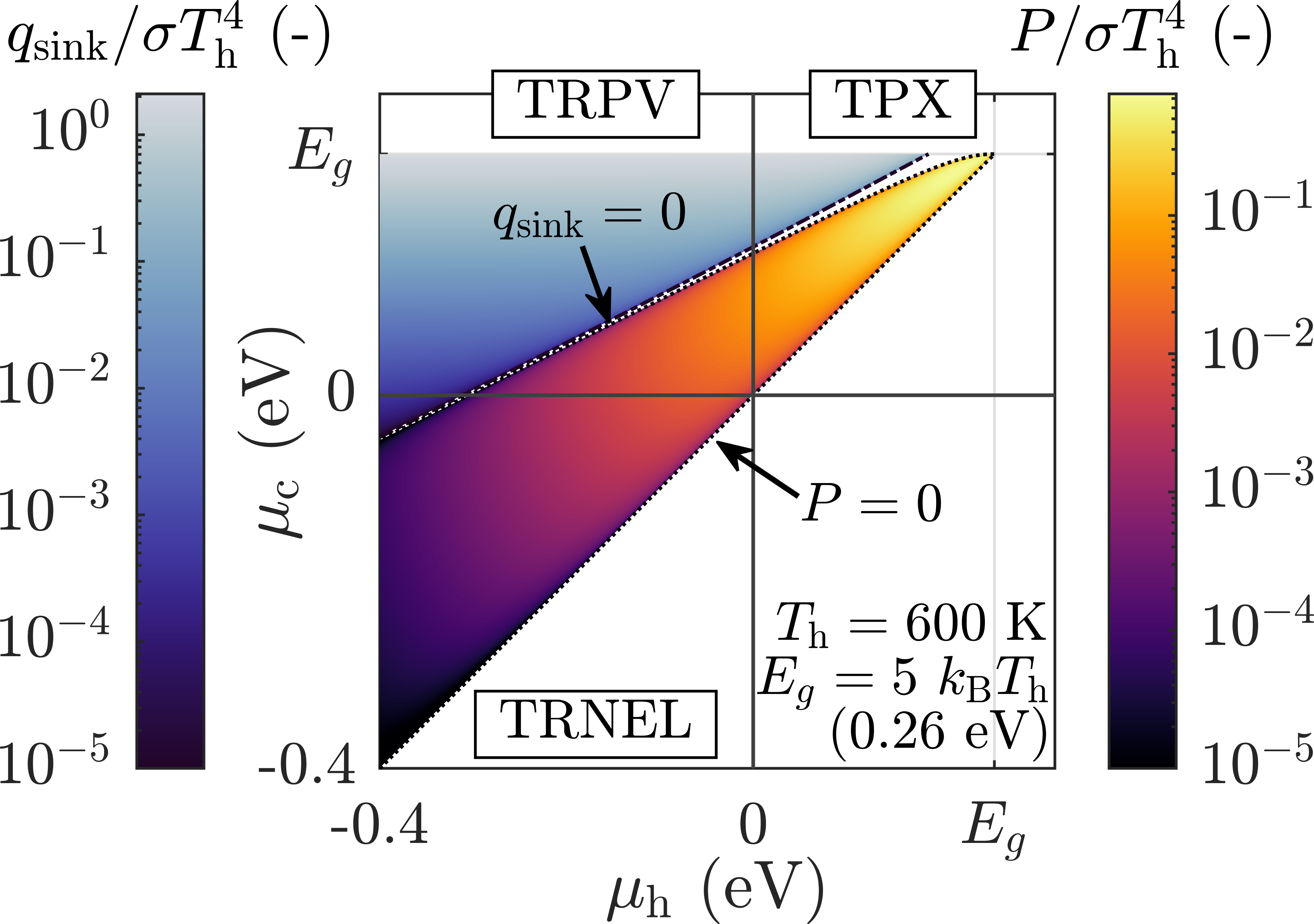
(a)

(b)

Figure 2: (a) Performance of dual radiative systems operating as heat engines or heat pumps, at the radiative limit and for $E_{g}=5k_{\mathrm{B}}T_{\mathrm{h}}=0.26$ eV. (b) Operating regions of dual radiative systems in the limit of an infinite bandgap.

For the bandgap selected, the dual system is able to operate both as a heat engine and a heat pump in three of the four quadrants: namely, the TPX quadrant (upper-right), the TRPV quadrant (upper-left) but also the “TRNEL” quadrant, in which a cold negative electroluminescent (NEL) diode consumes electrical power to limit the radiation sent to the hot facing TR cell. To the best of our knowledge, the TRNEL device has never been mentioned in literature. Globally, both the power output and the cooling power increases with $\mu_{\mathrm{c}}$, while $P$ also increases with $\mu_{\mathrm{h}}$: the maximum power point (MPP) is therefore located in the TPX quadrant, while the maximum cooling power is reached in TRPV operation for $\mu_{\mathrm{c}}\rightarrow E_{g}$. Despite $\mu_{\mathrm{c}}\rightarrow E_{g}$, the cooling power converges towards a constant value, as demonstrated in [28]. Additionally, note that for low $E_{g}$, the TPX device becomes unable to perform cooling (see Section II of Supp. Mat. [10]).

Note how the dual system does not switch directly from heat engine to heat pump operation as $\mu$ varies. Indeed, there is a narrow region in-between where the system is neither able to generate electrical power nor to cool the cold source. This gap can especially be observed when $E_{g}-\mu_{h}$ becomes lower than $k_{\mathrm{B}}T_{\mathrm{h}}$, but globally narrows down as the bandgap increases: in the limit of infinite bandgaps, the two operating regions become adjacent as $q_{\mathrm{h}}=q_{\mathrm{c}}$ and $\dot{N}_{\mathrm{h}}=\dot{N}_{\mathrm{c}}$ are equivalent. This is schematised in Fig. 2(b). In this situation, the term related to the lowest-order polylogarithm dominates in the expressions provided in Eq. (2). By linearising $\operatorname{Li}_{1}$, we obtain that the transition from one region to the other - which corresponds to open-circuit conditions - occurs approximately for

$$\mu_{\mathrm{c}}=\frac{T_{\mathrm{c}}}{T_{\mathrm{h}}}\mu_{\mathrm{h}}+\left(1-\frac{T_{\mathrm{c}}}{T_{\mathrm{h}}}\right)E_{g}+k_{\mathrm{B}}T_{\mathrm{c}}\ln\left(\frac{T_{\mathrm{h}}}{T_{\mathrm{c}}}\right),$$ (6)

this linearised expression being a very good approximation as long as $E_{g}-\mu_{i}\gg k_{\mathrm{B}}T_{i}$. The other side of the power production region is simply delimited by the condition $\mu_{\mathrm{h}}=\mu_{\mathrm{c}}$. These two expressions have already been mentioned for TPX devices in [20].

To quantify and compare the performance of TPX, TRPV and TRNEL devices, we provide in Fig. 3 the $\eta-P$ plots obtained by varying both $\mu_{\mathrm{h}}$ and $\mu_{\mathrm{c}}$, considering three different bandgaps and a heat source temperature of 600 K. For each device, the shaded area corresponds to achievable operation, while the full line is the envelope of this area. Looking at the three cases considered, it is first interesting to notice that while the shape of the admissible $\eta-P$ area changes significantly when considering each engine individually, it remains mostly unchanged with varying bandgaps for the full dual radiative engine. For any of the bandgaps considered, the efficiency at maximum power remains mostly constant (between 28% and 34% of the Carnot efficiency $\eta_{\mathrm{C}}=1-T_{\mathrm{c}}/T_{\mathrm{h}}$), while the maximum efficiency is always $\eta_{\mathrm{C}}$ and is reached at zero power.

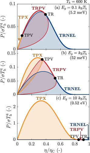
Figure 3: $\eta-P$ plots of dual radiative engines at the radiative limit, for $T_{\mathrm{h}}=600$ K and for various bandgaps.

If we now compare the different engines, TRNEL appears to be the optimal choice to maximise the efficiency, being always able to reach the Carnot efficiency. Note that this is true only because it operates at the radiative limit: in Section III of Supp. Mat. [10], we analyse the impact of non-radiative losses on performance by considering a spectrally flat quantum efficiency, and pinpoint that the interest of TRNEL operation vanishes when the quantum efficiency goes significantly below unity. Even at the radiative limit, the advantage of TRNEL operation shrinks for large bandgap: as $E_{g}\rightarrow\infty$, all radiative engines are able to approach the Carnot efficiency in open-circuit conditions. This has already been demonstrated for TR [6, 7] and TPV [29], but can in fact be shown for any radiative engine. In the limit of an infinite bandgap $(q_{\mathrm{h}}-q_{\mathrm{c}})/(\dot{N}_{\mathrm{h}}-\dot{N}_{\mathrm{c}})\rightarrow E_{g}$, leading $\eta$ to be expressed as $(\mu_{\mathrm{c}}-\mu_{\mathrm{h}})/(E_{g}-\mu_{\mathrm{h}})$. Using Eq. (6), and keeping in mind that $E_{g}-\mu_{\mathrm{h}}\gg k_{\mathrm{B}}T_{\mathrm{h}}$, we obtain that the efficiency in open-circuit conditions equals $\eta_{\mathrm{C}}$.

In contrast, to maximise the power output, TPX is almost always the best candidate, TRPV becoming optimal only for very low bandgap energies (here, for $E_{g}<k_{\mathrm{B}}T_{\mathrm{h}}\approx 0.05$ eV) which are not achievable physically. This remains true for lower or higher heat source temperatures (see Section IV of Supp. Mat. [10]). TPX devices generally outperform other radiative engines in terms of power output because the hot emitter operates as an LED: it is therefore able to largely enhance its emission by electroluminescence, increasing consequently the various energy flows in the system. For high enough bandgaps, this can even cause $P_{\mathrm{max}}$ to exceed $\sigma T_{\mathrm{h}}^{4}$ (see Fig. 3c), which is physically impossible for single radiative engines.

While TRNEL devices allow maximising efficiency and TPX devices power, TRPV systems can in some conditions provide interesting trade-offs between power and efficiency (see Fig. 3b). However, this can only be observed for low bandgaps (a few $k_{\mathrm{B}}T_{\mathrm{h}}$ at most) which are hardly achievable for the heat source temperature considered.

The study of $\eta-P$ plots directly highlights that the maximum efficiency of dual radiative engines is always the Carnot efficiency, reached for zero power output. Regarding the MPP, it was observed that $P_{\mathrm{max}}$ increases significantly with $E_{g}$ while $\eta_{\mathrm{MPP}}$ varies only slowly, but no analytical expressions of these quantities have yet been formulated. Therefore, in the following, we focus on the analytical derivation of $P_{\mathrm{max}}$ and $\eta_{\mathrm{MPP}}$. To do so, we consider once again that $E_{g}\rightarrow\infty$, since this allows reaching the largest possible power output (see Section V of Supp. Mat. [10]). By doing so, the $\operatorname{Li}_{1}$ term dominates the expressions provided in Eq. (2). Using that $\mu_{\mathrm{c}}-\mu_{\mathrm{h}}=x_{\mathrm{h}}k_{\mathrm{B}}T_{\mathrm{h}}-x_{\mathrm{c}}k_{\mathrm{B}}T_{\mathrm{c}}$, and defining $X_{i}$ as $\exp(-x_{i})$, the power output can be expressed as:

$$\begin{split}P=\frac{E_{g}^{2}k_{\mathrm{B}}^{2}T_{\mathrm{h}}^{2}}{4\pi^{2}c^{2}\hbar^{3}}&\left(\ln(X_{\mathrm{h}})-\frac{T_{\mathrm{c}}}{T_{\mathrm{h}}}\ln(X_{\mathrm{c}})\right)\times\\ &\left(\ln(1-X_{\mathrm{h}})-\frac{T_{\mathrm{c}}}{T_{\mathrm{h}}}\ln(1-X_{\mathrm{c}})\right),\end{split}$$ (7)

since $\operatorname{Li}_{1}(x)=\ln(1-x)$. By using the symmetry of this expression with respect to $X_{\mathrm{h}}$ and $X_{\mathrm{c}}$, one can show that $P$ reaches its maximum for $X_{\mathrm{h}}=X_{\mathrm{c}}=1/2$, thus for $\mu_{i}=E_{g}-\ln(2)k_{\mathrm{B}}T_{i}$ (see Section VI of Supp. Mat. [10]). Consequently, the maximum power output is

$$P_{\mathrm{max}}=\frac{1}{\hbar}\left(\frac{\ln(2)E_{g}k_{\mathrm{B}}(T_{\mathrm{h}}-T_{\mathrm{c}})}{2\pi c\hbar}\right)^{2},$$ (8)

and varies quadratically with both the bandgap energy and the temperature difference. Such variations were already pointed out in [28], although without a complete closed-form expression. Since $E_{g}\gg k_{\mathrm{B}}T_{i}$, both chemical potentials are greater than 0 and the maximum is reached in TPX regime, consistently with the results from Fig. 3.

To derive a closed-form expression of the efficiency at maximum power, we use that $x_{\mathrm{h,MPP}}=x_{\mathrm{c,MPP}}=\ln(2)$ to obtain $(\mu_{\mathrm{c,MPP}}-\mu_{\mathrm{h,MPP}})/(E_{g}-\mu_{\mathrm{h,MPP}})=\eta_{\mathrm{C}}$. Dividing both the numerator and the denominator of Eq. (5) by $(\dot{N}_{\mathrm{h}}-\dot{N}_{\mathrm{c}})(E_{g}-\mu_{\mathrm{h}})$, one gets

$$\eta_{\mathrm{MPP}}=\frac{\eta_{\mathrm{C}}}{1+\left(\frac{1}{\rho}-1\right)\frac{1}{\ln(2)}\frac{E_{g}}{k_{\mathrm{B}}T_{\mathrm{h}}}},$$ (9)

where $\rho=E_{g}(\dot{N}_{\mathrm{h}}-\dot{N}_{\mathrm{c}})/(q_{\mathrm{h}}-q_{\mathrm{c}})$ corresponds to the fraction of radiative energy being useful to optoelectronic conversion. To express it, both $\operatorname{Li}_{1}$ and $\operatorname{Li}_{2}$ terms are necessary. One obtains

$$\left(\frac{1}{\rho}-1\right)\frac{1}{\ln(2)}\frac{E_{g}}{k_{\mathrm{B}}T_{\mathrm{h}}}\underset{E_{g}\rightarrow\infty}{\sim}(2-\eta_{\mathrm{C}})\frac{1}{\ln(2)}\frac{\operatorname{Li}_{2}(1/2)}{\operatorname{Li}_{1}(1/2)}.$$ (10)

The polylogarithmic terms having closed-form expressions for $x=1/2$, the efficiency at maximum power obtained as $E_{g}\rightarrow\infty$ is

$$\eta_{\mathrm{MPP,}E_{g}\rightarrow\infty}=\frac{\eta_{\mathrm{C}}}{1+(2-\eta_{\mathrm{C}})\chi},$$ (11)

$\chi$ being a constant equal to $\frac{1}{2}\left(\frac{1}{6}\left(\frac{\pi}{\ln(2)}\right)^{2}-1\right)\approx 1.21$. The temperature variation of $\eta_{\mathrm{MPP,}E_{g}\rightarrow\infty}$ is provided in Fig. 4 (black line), and matches well the numerical results obtained for bandgaps larger than $100k_{\mathrm{B}}T_{\mathrm{h}}$. It also gives a good estimate of the efficiency obtained for standard bandgaps, as long as $E_{g}\gg k_{\mathrm{B}}T_{\mathrm{h}}$: for $T_{\mathrm{h}}=600$ K, $\eta_{\mathrm{MPP},E_{g}\rightarrow\infty}=17.7$% while $\eta_{\mathrm{MPP,1\;eV}}=$17.1% and $\eta_{\mathrm{MPP,0.52\;eV}}=16.6$%.

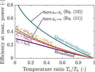
Figure 4: Variation of the efficiency at maximum power with the heat source temperature. For simplicity, only the TPX quadrant has been considered.

To better understand how efficient dual radiative engines are at maximum power, one can compare Eq. (11) with classical upper bounds for $\eta_{\mathrm{MPP}}$. We choose to perform the comparison with the Novikov-Curzon-Ahlborn [30, 31] efficiency $\eta_{\mathrm{NCA}}=1-\sqrt{T_{\mathrm{c}}/T_{\mathrm{h}}}$ and the Schmiedl-Seifert [32] efficiency $\eta_{\mathrm{SS}}=2\eta_{\mathrm{C}}/(4-\eta_{\mathrm{C}})$, which were found to be efficiency bounds for endoreversible and exoreversible thermoelectric generators respectively [33]. For the temperatures previously considered, both efficiencies are close to 29%, hence 11 percent points higher than $\eta_{\mathrm{MPP,}E_{g}\rightarrow\infty}$. This significant difference, which highlights the presence of additional losses in radiative engines, can be attributed to thermalisation losses - i.e., to the fraction of radiative energy exchanged which is useless to optoelectronic conversion. To prove this, we now consider that the radiation is quasi-monochromatic around $E_{g}$, which makes the ratio $\rho$ equal to 1. In this scenario, $\mu_{i\mathrm{,MPP}}$ is found to tend towards $E_{g}$ (see Section VII of Supp. Mat. [10]). Then, the Bose-Einstein distributions can be simplified using that $[\exp(x)-1]^{-1}\sim x^{-1}$ around 0. Setting any of the two partial derivatives of $P$ with respect to $\mu_{i}$ to zero leads to

$$\eta_{\mathrm{MPP,}\hbar\omega=E_{g}}=1-\sqrt{\frac{T_{\mathrm{c}}}{T_{\mathrm{h}}}},$$ (12)

exactly the Novikov-Curzon-Ahlborn efficiency. $\delta E$ being the radiation spectral bandwidth, the maximum power output is then

$$P_{\mathrm{max}}=\frac{1}{\hbar}\left(\frac{E_{g}\sqrt{k_{\mathrm{B}}}(\sqrt{T_{\mathrm{h}}}-\sqrt{T_{\mathrm{c}}})}{2\pi c\hbar}\right)^{2}\delta E,$$ (13)

an expression similar to Eq. (8). Since $P$ goes to zero as $\delta E\rightarrow 0$, there is a trade-off between power and efficiency as the bandwidth varies, as illustrated in Fig. 5: to achieve non-zero output power, the efficiency must fall below the usual bounds. It is noteworthy that the efficiency starts to decrease for bandwidths as low as few meV (corresponding to a quality factor $Q=E_{g}/\delta E$ close to 100 for $E_{g}=0.52$ eV), while reaching the broadband limit for a bandwidth of few tenths of eV (i.e. for $Q\approx 1$ considering $E_{g}=0.52$ eV). If the efficiency at maximum power is too low for a given application, two main leverages are thus available to increase it, although at the expense of power: decrease the radiation bandwidth, or change $\mu_{\mathrm{h}}$ and $\mu_{\mathrm{c}}$ to move in the broadband $\eta-P$ plots provided in Fig. 3, which can allow exceeding the aforementioned bounds [4]. The interest of each of these leverages depends on the bandgap, and on how far the system operates from the radiative limit. In some cases, spectral filtering can allow extending the region of achievable operating conditions, limiting the power loss undergone when high efficiency is required (see Section VIII of Supp. Mat [10]).

Figure 5: Variation of the maximum power and related efficiency for varying spectral bandwidth, considering $T_{\mathrm{h}}=600$ K. For simplicity, only the TPX quadrant has been considered.

In conclusion, we have studied the power output and efficiency achievable by dual radiative heat engines, especially when they operate at the radiative limit. A unified view allows shining light on their similarities and respective merits. In particular, TRNEL devices are found to systematically reach Carnot efficiency, while TPX devices are almost always the best dual engines in terms of power output, and offer the broadest range of operating conditions of all dual engines for bandgaps over a few $k_{\mathrm{B}}T_{\mathrm{h}}$. We have analytically derived an upper bound for the maximum power and related efficiency, the latter mostly lying between 30% and 40% of $\eta_{\mathrm{C}}$ and being several percent points below usual efficiency bounds due to thermalisation losses (11 points below for $T_{\mathrm{h}}=600$ K). Interestingly, spectral filtering can mitigate part of the power loss when high efficiencies are targeted. In practice, below-bandgap radiation, more rigorous non-radiative losses and resistive losses shall be included, as well as thermal resistance effects at the thermostats which reduce the operating temperature difference $T_{\mathrm{h}}-T_{\mathrm{c}}$ [23]. In addition, it would be worth investigating how the performance of such engines changes in the near field, where radiative emission exceeds the modified Planck law [19, 20, 23].