Abstract

The use of machine-learning techniques has grown in numerous research areas. Currently, it is also widely used in statistics, including the official statistics for data collection (e.g. satellite imagery, web scraping and text mining, data cleaning, integration and imputation) but also for data analysis. However, the usage of these methods in survey sampling including small area estimation is still very limited. Therefore, we propose a predictor supported by these algorithms which can be used to predict any population or subpopulation characteristics based on cross-sectional and longitudinal data. Machine learning methods have already been shown to be very powerful in identifying and modelling complex and nonlinear relationships between the variables, which means that they have very good properties in case of strong departures from the classic assumptions. Therefore, we analyse the performance of our proposal under a different set-up, in our opinion of greater importance in real-life surveys. We study only small departures from the assumed model, to show that our proposal is a good alternative in this case as well, even in comparison with optimal methods under the model. What is more, we propose the method of the accuracy estimation of machine learning predictors, giving the possibility of the accuracy comparison with classic methods, where the accuracy is measured as in survey sampling practice. The solution of this problem is indicated in the literature as one of the key issues in integration of these approaches. The simulation studies are based on a real, longitudinal dataset, freely available from the Polish Local Data Bank, where the prediction problem of subpopulation characteristics in the last period, with "borrowing strength" from other subpopulations and time periods, is considered.

KEYWORDS: Machine learning; Survey sampling; Small area estimation; Plug-in predictors; Bootstrap

1 Introduction

Model-based approach in survey sampling and small area estimation can be used to make an inference on population and subpopulation characteristics based on data from random and non-random samples, including longitudinal surveys, web surveys, and integrated datasets obtained from different sources. In contrast to conventional econometrics applications, the objective of the analysis is not the prediction of a random variable (for a future period or for an unobserved population element), but rather the prediction of a specific function of random variables in a population or subpopulation. Examples of such functions can be their linear combination, such as the mean, or more complex functions such as quantiles. This approach requires making assumptions about the population distribution of the variable under study, called – in survey sampling – the superpopulation model (see e.g. Valliant et al.,, 2000) or shortly the model.

In the model-based approach, it is possible to find optimal predictors under the assumed model. Different classes of optimal predictors are considered in the literature. If the problem of prediction of any linear combination of the variable of interest is analysed, the Best Linear Unbiased Predictors (BLUPs) and their estimated versions called the Empirical Best Linear Unbiased Predictors (EBLUPs), can be used. BLUPs, considered for example by Henderson, (1950) and Royall, (1976), are predictors which minimises the Mean Squared Error (MSE) in the class of unbiased predictors. The difference between the MSE of the EBLUP and the MSE of the BLUP, resulting from the estimation of model parameters, is usually very small. For example, in simulation studies conducted by Żądło, (2006) based on a dataset from the Polish agriculture census, the obtained MSEs of EBLUPs are higher only by $0.03\%-1.1\%$ comparing with the MSEs of BLUPs. Hence, it is very difficult to find predictors more accurate than EBLUPs in the class of unbiased predictors under the correctly specified model. The overview of various EBLUPs modifications, including Spatial EBLUPs (Pratesi and Salvati,, 2008; Molina et al.,, 2009) and Geographically Weighted EBLUP (e.g. Chandra et al.,, 2012), is presented in the third chapter of Krzciuk, (2024).

If the objective is to predict not only the linear combination but any function of the variable of interest minimising the MSE, the Best Predictor (BP), studied for example by Molina and Rao, (2010), can be considered. Hence, the BP is a very useful predictor, but it requires very strong (distributional) assumptions to be met, which is not necessary for the EBLUP. Its estimated version, obtained by replacing parameters usually by their residual maximum likelihood estimators, is called the Empirical Best Predictor (EBP). A different approach to the estimation process of model parameters in the case of the BP leading to the Observed BP is proposed by Jiang et al., (2011), and then developed by Sugasawa et al., (2019) to include the process of model selection, which gives the Observed Best Selective Predictor (OBSP). In contrast to the differences between the MSEs of EBLUPs and BLUPs, the difference between the MSE of EBP and the MSE of BP can be large. In simulation studies presented by Chwila and Żądło, (2022) based on real data from U.S. Census Bureau, the obtained MSEs of EBPs under correctly specified Linear Mixed Model (LMM) are higher by $0.3\%-188.2\%$ comparing with the MSEs of BPs. Therefore, due to possible even very high differences between the accuracy of the BP and its estimated version, it is purposeful to look for predictors more accurate than the EBP. Chwila and Żądło, (2022) show that in many cases the PLUG-IN predictors under the LMM are more accurate (or have similar accuracy) compared with the EBPs. Hence, further studies on the PLUG-IN predictors, which allow to predict any function of the variable of interest (even the distribution function - see e.g. Stachurski,, 2021) and, at the same time, do not require strong distributional assumptions, should be performed. This class of predictors, with an additional property of robustness on model misspecification, is of our interest.

Machine learning methods can offer several advantages over linear models, especially when the deviations from the linear models assumptions are meaningful. They can model complex nonlinear relationships, automatically capture interaction effects between variables and outlier observations, whereas in classic linear models these would need to be manually specified. Kontokosta et al., (2018), Chen et al., (2019) and Jumin et al., (2020) show the advantage of the methods over the linear model in the case of different prediction problems. Because the performance of the methods in the case of strong and moderate departures of classic assumptions is known, the performance of the proposed predictor under a different setup, considering small deviations from the assumed model, will be analysed. This issue is crucial for practitioners who are usually conscious of strong or moderate departures from the classic assumptions, but are interested in the performance of the methods they employ (including optimal predictors under the assumed model) and their alternatives when the deviations from the model can be difficult to identify.

Furthermore, it is noteworthy that the assessment of machine learning methods, discussed e.g. in James et al., (2013, p. 29-30) and Hastie et al., (2009, pp. 241-249), is conducted in a distinct manner than the accuracy assessment in the model-based approach in survey sampling. Hence, integration of the machine learning and model-based methods used in survey sampling requires the ability of the assessment of prediction accuracy of machine learning methods following the approach used in survey sampling.

Summing up, there are the following aims of the paper:

• the proposal of a plug-in predictor of any population or subpopulation characteristic based on one of machine learning methods, which can be used for longitudinal data,

• the comparison of its properties and properties of classic methods, including optimal predictors, based on Monte Carlo simulation study under small departures from the assumed model,

• proposals of estimators (parametric, residual and double bootstrap) of prediction-accuracy measures based on quantiles of absolute prediction errors of the proposed predictor under the model of interest,

• the Monte Carlo comparative simulation studies of the properties of the prediction-RMSE estimators and the proposed quantile-based accuracy measures estimators of the proposed predictor and other predictors.

2 Survey sampling and machine-learning

In the previous section, we have introduced the aims of the paper against the background of model-based survey sampling methods. In this section, we present a review of the literature on the use of machine learning methods in survey sampling.

According to Corral et al., (2022, p. 5) machine learning methods has become popular among academics and policymakers after the publication of Jean et al., (2016) who demonstrated that obtaining socioeconomic information from high-resolution daytime satellite images can help in precise estimation of poverty and wealth. In 2018, a survey on the use of machine learning in official statistics was conducted by the Federal Statistical Office of Germany (Beck et al.,, 2018) among 33 national statistical offices, Eurostat, and the OECD. Of those surveyed, 21 institutions reported running projects using machine learning techniques, but primarily for data collection and preparation. The usage of the machine learning methods for the inference on the population or subpopulation characteristics, as well as the accuracy assessment – considered in this paper – was not reported. In the same year, researchers from the UK and Germany proposed a general framework for the process of producing small area statistics (Tzavidis et al.,, 2018). Similar problems were also discussed by De Broe et al., (2020). In both publications, Authors note the relatively low use of machine learning methods in survey sampling compared to other applications. As the key issue, they define the problem considered in our paper – the ability to obtain correct uncertainty estimates for the considered estimators or predictors.

According to Meertens et al., (2022), "currently, a paradigm shift from a data modelling culture to an algorithmic modelling culture, as envisioned by Breiman, (2001), is taking place in the field of official statistics (De Broe et al.,, 2020)". In 2021, a paper addressing the use of machine learning techniques from a public statistics perspective was published (Puts and Daas,, 2021). The Authors noted that machine learning methods can be used to extract information from images and text, which can be particularly useful for official statistics. Ashofteh and Bravo, (2021) claimed that the role of longitudinal models and machine learning methods, which we consider in this paper, for official statistics will be increasing. The same year, a report (UNECE,, 2021) on the use of machine learning in the production of official statistics was published with similar conclusions. The Authors see the integration challenges as the critical step in the further development of these methods within the official statistics. Issues considered in this paper can help to solve this problem. The proposed procedure of prediction accuracy estimation (as it is understood in survey sampling) of new machine learning methods is absolutely essential in practice. It is a crucial step for implementation of the theoretical concept of new predictors in the production of statistics, including the acceptance of the methods by data users. It is because it allows for comparisons with standard methods already used in real surveys.

The use of a machine learning for small area estimation purposes is an issue that has been considered in the literature in recent years. In some papers (see Robinson et al.,, 2017; Kontokosta et al.,, 2018; Singleton et al.,, 2020) Authors use a fully machine learning-based approach for prediction in subpopulations, usually based on data at the subpopulation-level. Their approach is distant from small area estimation methods, and the estimation of prediction accuracy following survey sampling methodology is not considered. The methodology similar to our approach is studied by Krennmair and Schmid, (2022). They propose a new machine learning model – a random forest with the addition of random effects, effects that are commonly used for small area statistics problems. The Authors propose an algorithm to fit the model, the predictor of the small area mean, which can be treated as the generalization of the EBLUP, and the method, similar to the residual bootstrap, of the prediction accuracy estimation under the proposed model. In contrast, our approach allows to predict not only the subpopulation mean but any function of the population (or subpopulation) vector of the variable of interest and compare the prediction accuracy of our method with competitors based on any specified model. What should be noted, for the problem of subpopulation mean prediction in nonsampled areas our predictor simplifies to the predictor proposed by Krennmair and Schmid, (2022, p. 1872).

Dagdoug et al., (2023) present a model-assisted (not model-based) proposal which can be treated as an alternative solution but only for estimation of the population total. The proposed estimators are generalisations of the generalized regression (GREG) estimator considered by Deville and Särndal, (1992). The Authors replace parametric model-based fitted values in the formula of GREG by values which can be fitted by any parametric or nonparametric procedure. Their proposal can be easily modified to apply the machine-learning for the estimation of the subpopulation total as well. Rao and Molina, (2015) in chapters 2.4.2, 2.4.3 and 2.5 present how to modify GREG of the population total to obtain three calibration estimators of the subpopulation totals: with population-specific auxiliary information (given there by equation (2.4.8)), domain-specific auxiliary information (given by (2.4.11)) and modified GREG (given by (2.5.1)). Their formulae can be written as functions of fitted values of a linear model, denoted in Rao and Molina, (2015) by: $\hat{y}_{j}$ in (2.4.8), $\mathbf{x}_{j}\mathbf{\hat{B}}_{i}$ in (2.4.11) (see the description of all notations below this equation), and $\mathbf{x}_{j}\mathbf{\hat{B}}$ in (2.5.1), where subscript $j$ and $i$ are used to denote the $j$th sampled element and the $i$th subpopulation, respectively. If in these formulae values fitted by a linear model are replaced by values fitted by any model (including machine-learning algorithms), the appropriate generalization will be obtained. What is more, Dagdoug et al., (2023) derive the design-variance estimator of their estimator and study its properties in the design-based simulation analyses.

The next two sections will introduce the proposed methodology. In Section 3 we will propose a machine learning-based PLUG-IN predictor of any function of the population vector of the variable of interest that can be used both for cross-sectional and longitudinal surveys. In Section 4 we will present our proposal for an accuracy estimation procedure of the predictor.

3 Models and predictors

Let the random variable of interest for the $t$ period ($t=1,2,\dots,M$) and the $i$th population element ($i=1,2,\dots,N_{t}$), be denoted by $Y_{it}$, where $M$ and $N_{t}$ are the number of time periods (possibly including the considered future periods) and the population size in the $t$th period, respectively. Let $N_{(L)}=\sum_{t=1}^{M}{N_{t}}$. In a special case, when the population does not change in $M$ considered periods ($\forall t~{}N_{t}=N$), then $N_{(L)}=N\times M$. When only cross-sectional population data are considered ($M=1$), we obtain $N_{(L)}=N$. We assume that random or non-random longitudinal sample data are available, where the number of observed cases will be denoted by $n_{(L)}$.

Let the population vector of random variables of interest $Y_{it}$, where $t=1,2,\dots,M$ and $i=1,2,\dots,N_{t}$, of size $N_{(L)}\times 1$ be denoted by $\mathbf{Y}$. Let the fixed (non-random) matrix of auxiliary variables of size $N_{(L)}\times p$ be denoted by $\mathbf{X}$.

Let us assume that

$$\left\{\begin{array}[]{c}\mathbf{Y}=m(\mathbf{X})+\boldsymbol{\xi}\\ E(\boldsymbol{\xi})=\mathbf{0}\\ Var(\boldsymbol{\xi})=\mathbf{V}\end{array}\right.,$$ (1)

where $m$ is some fixed but unknown function of auxiliary variables, $\boldsymbol{\xi}$ is a random term with $\mathbf{0}$ mean and unknown variance-covariance matrix $\mathbf{V}$. What is important, the formula (1) covers many models. Let us consider two special cases. Firstly, in machine-learning procedures, see Hastie et al., (2009, p. 28), usually (1) is considered, where the independence of elements of $\boldsymbol{\xi}$ is additionally assumed. Secondly, the General Linear Mixed Model, which special cases will be analyzed in Section 5.1, can also be written as (1). It is given by (e.g. Rao and Molina, (2015), p. 98):

$$\left\{\begin{array}[]{c}\mathbf{Y}=\mathbf{X}\boldsymbol{\beta}+\mathbf{Z}\mathbf{v}+\mathbf{e}\\ E(\mathbf{e})=\mathbf{0},E(\mathbf{v})=\mathbf{0}\\ Var(\mathbf{e})=\mathbf{R}(\boldsymbol{\delta}),Var(\mathbf{v})=\mathbf{G}(\boldsymbol{\delta})\end{array}\right.,$$ (2)

where $\boldsymbol{\beta}$ is a vector of fixed effects of size $p\times 1$ and $\boldsymbol{\delta}$ is a vector of parameters called the variance components. The random part of the model is described by: a known matrix $\mathbf{Z}$ of size $N_{(L)}\times h$, a vector $\mathbf{v}$ of random effects of size $h\times 1$ and a vector $\mathbf{e}$ of random components of size $N_{(L)}\times 1$, where $\mathbf{e}$ and $\mathbf{v}$ are assumed to be independent. Hence, defining in (1):

• $\boldsymbol{\xi}$ as $\mathbf{Z}\mathbf{v}+\mathbf{e}$ (see the random term in (2)),

• and $m(\mathbf{X})$ as $\mathbf{X}\boldsymbol{\beta}$ (see the fixed term in (2))

shows that (2) is a special case of (1), where $\mathbf{V}$ in (1), using the notation used in (2), is given by: $\mathbf{V}=\mathbf{Z}\mathbf{G}\mathbf{Z}^{T}+\mathbf{R}$.

Let us assume, without the loss of generality, that the first $n_{(L)}$ elements of $\mathbf{Y}$ are for the sample elements. Then, we can decompose the random vector $\mathbf{Y}$ into the observed and non-observed subvectors: $\mathbf{Y}=[\mathbf{Y}_{s}^{T}~{}\mathbf{Y}_{r}^{T}]^{T}$, where $\mathbf{Y}_{s}$ and $\mathbf{Y}_{r}$ are of sizes $n_{(L)}\times 1$ and $(N_{(L)}-n_{(L)})\times 1$, respectively. Similarly, we can decompose matrices $\mathbf{X}$ and $\mathbf{Z}$ into: $\mathbf{X}=[\mathbf{X}_{s}^{T}~{}\mathbf{X}_{r}^{T}]^{T}$ and $\mathbf{Z}=[\mathbf{Z}_{s}^{T}~{}\mathbf{Z}_{r}^{T}]^{T}$, where $\mathbf{X}_{s}$, $\mathbf{Z}_{s}$, $\mathbf{X}_{r}$ and $\mathbf{Z}_{r}$ are of sizes $n_{(L)}\times p$, $n_{(L)}\times h$, $(N_{(L)}-n_{(L)})\times p$ and $(N_{(L)}-n_{(L)})\times h$, respectively.

Let us consider the problem of prediction of any given function of the population vector of the variable of interest $\theta=\theta(\mathbf{Y})=\theta([\mathbf{Y}_{s}^{T}~{}\mathbf{Y}_{r}^{T}]^{T})$. We consider the PLUG-IN predictor, which for a given $\theta$ is defined as:

$$\hat{\theta}=\theta([\mathbf{Y}_{s}^{T}~{}\hat{m}(\mathbf{X}_{r}^{T})]^{T})$$ (3)

where $\hat{m}(\mathbf{X}_{r})$ is a $(N_{(L)}-n_{(L)})\times 1$ vector of fitted values, based on any assumed model, for non-observed random variables. The vector construction will be discussed for two special cases: the General Linear Mixed Model and machine learning algorithms in the following paragraphs in this section.

In the case of the General Linear Mixed Model the fitted values of non-observed random variables, denoted in (3) by $\hat{m}(\mathbf{X}_{r})$, are defined as follows $\hat{m}_{GLMM}(\mathbf{X}_{r})=\mathbf{X}_{r}\hat{\boldsymbol{\beta}}+\mathbf{Z}_{r}\hat{\mathbf{v}}$, where $\hat{\boldsymbol{\beta}}$ and $\hat{\mathbf{v}}$ are given by the formulae of the best linear unbiased estimator of $\boldsymbol{\beta}$ and the best linear unbiased predictor of $\mathbf{v}$ (see Rao and Molina, (2015, p. 98) for more details), respectively, where unknown variance components $\boldsymbol{\delta}$ are replaced by their estimates (e.g. Restricted Maximum Likelihood estimates). What is interesting, the formula of $\hat{m}_{GLMM}(\mathbf{X}_{r})$ covers not only $\mathbf{X}_{r}\hat{\boldsymbol{\beta}}$ but also $\mathbf{Z}_{r}\hat{\mathbf{v}}$ which results from the assumptions (1), where the random part of the model $\boldsymbol{\xi}=\mathbf{Z}\mathbf{v}+\mathbf{e}$ can cover spatial or temporal correlations.

In machine learning, as stated in James et al., (2013, p. 17), $\hat{m}(.)$ represents an estimate for $m(.)$, usually treated as a black box in the sense that the form of $\hat{m}(.)$ is not of primary interest as opposed to goodness-of-fit and prediction accuracy. Although, any machine learning method can be used, we consider gradient-boosting regression trees – one of the most popular algorithms used for regression problems. It is due to its very good prediction results for real data applications (i.e. Kaggle competitions), relatively low computation time (for example in comparison with neural networks) and the fact that the algorithm does not require additional data preprocessing like other machine learning methods (including data standardization). The algorithm was introduced simultaneously in 1999 by Jerome H. Friedman (Friedman,, 2001) and four researchers: Llew Mason, Jonathan Baxter, Peter Bartlett and Marcus Frean (Mason et al.,, 2001).

The decision tree in its basic structure divides data many times into segments (leaves), accordingly to certain cut-off values determined for auxiliary variables (see Hastie et al.,, 2009, chapter 9.2). The gradient boosting (GB) algorithm is an enhanced version of the decision tree model: the trees are built many times, based on the subsamples of variables and records, during an iterative procedure. The applied GB trees algorithm can be presented in the following steps (Hastie et al.,, 2009).

1. Select the train dataset, the subsample size is defined by the researcher (i.e. 70% of the sample size).

2. For the subsample drawn in the previous step, the decision tree is fitted with CART algorithm (Breiman et al.,, 1984). During each following split of the single segment into two separate leaves, the different, randomly drawn subsample of the auxiliary variables is considered (i.e. 80% of variables). The subsample size of auxiliary variables is defined by the researcher.

3. After the creation of a tree in the $b$th step, the fitted values $\hat{\mathbf{y}}_{b}$ for each observation in the train dataset are calculated.

4. The fitted values are multiplied by a learning rate hyperparameter $\eta$ from range $[0,1]$ i.e. by $0.01$. The residuals of the model are calculated as follows:

   $$\mathbf{r}_{b}=\mathbf{y}-\eta\hat{\mathbf{y}}_{b}.$$

5. Vector $\mathbf{y}$ is replaced by the residuals obtained in the previous step: $\mathbf{y}=\mathbf{r}_{b}.$

6. The algorithm goes back to the first step. The steps (a)-(e) are repeated $B$ times, where $B$ is a defined hyperparameter, i.e. $B=500$.

7. The final form of the GB tree is given by:

   $$\hat{\mathbf{y}}_{boost}=\sum_{b=1}^{B}\eta\hat{\mathbf{y}}_{b}.$$

The hyperparameters of the model can be chosen based on the procedure of the K-folded cross-validation, where the decision is based on the averaged over cross-validation steps the test MSE (ex-post MSE), as discussed for example by James et al., (2013, pp. 181-183). The initial set of hyperparameters can be obtained with the so-called random search or grid search procedures, which allow to create a given number of randomly selected hyperparameters (see e.g. Swamynathan,, 2019, pp. 312-316). The hyperparameters with the lowest average ex-post MSE are chosen for parameters estimation based on the whole sample for the model creation purpose.

4 Prediction accuracy estimation

In our opinion, in order to integrate machine learning and small-area techniques, it is essential to be able to compare their accuracy in real-life surveys. Therefore, it is crucial to follow the survey methodology to make the comparison. In this section, we will introduce prediction accuracy measures, including our proposal, and procedures of their estimation applying the model-based approach in small area estimation and survey sampling.

4.1 Prediction accuracy measures

We consider the problem of prediction of any given function of the population vector $\mathbf{Y}$, denoted by $\theta=\theta(\mathbf{Y})$ by any predictor $\hat{\theta}$, including the PLUG-IN predictor given by $(\ref{plug_in})$. Our aim is to assess the accuracy of $\hat{\theta}$ under the Linear Mixed Model (LMM) given by (2) with additional assumption of normality of random effects and random components. However, this approach can be used for any model allowing for the generation of the population vector of the variable of interest, including generalized linear mixed models with logistic mixed model as a special case (González-Manteiga et al.,, 2007; Flores-Agreda and Cantoni,, 2019). Let the prediction error be defined as $U=\hat{\theta}-\theta$. The prediction Root MSE (RMSE) is given by

$$RMSE(\hat{\theta})=\sqrt{E(\hat{\theta}-\theta)^{2}}=\sqrt{E({{U}^{2}})}.$$ (4)

Because the MSE is the mean of positively skewed squared prediction errors, we will also use the prediction measure called the Quantile of Absolute Prediction Errors (QAPE) introduced and studied by Żądło, (2013) and Wolny-Dominiak and Żądło, (2022), and defined as:

$$QAPE_{p}(\hat{\theta})=\inf\left\{{x:P\left({\left|{{\hat{\theta}-\theta}}\right|\leq x}\right)\geq p}\right\}=\inf\left\{{x:P\left({\left|{{U}}\right|\leq x}\right)\geq p}\right\}.$$ (5)

Hence, this measure is the $p$th quantile of the absolute prediction error $|U|$. The above described accuracy prediction measures RMSE and QAPE can be estimated using different bootstrap techniques.

4.2 Parametric and residual bootstrap

The parametric bootstrap procedure is implemented according to González-Manteiga et al., (2007) and González-Manteiga et al., (2008) and presented in Appendix A. Based on the procedure, in $B$ iterations we obtain $B$ bootstrap realizations of the prediction errors given by:

$$u^{*(b)}=\hat{\theta}^{*(b)}-\theta^{*(b)}.$$ (6)

where $b=1,2,\dots,B$, $\theta^{*(b)}$ is the predicted characteristic computed based on the $b$th bootstrapped population vector of the variable of interest, and $\hat{\theta}^{*(b)}$ is its predictor computed based on the $b$th bootstrapped sample vector of the variable of interest.

The parametric bootstrap estimators of (4) and (5) are given respectively by:

$$\widehat{RMSE}(\hat{\theta})=\left(B^{-1}\sum_{b=1}^{B}u^{*(b)^{2}}\right)^{0.5}$$ (7)

and

$$\widehat{QAPE}_{p}(\hat{\theta})=q_{p}(|u^{*(1)}|,\dots,|u^{*(b)}|,\dots,|u^{*(B)}|),$$ (8)

where $u^{*(b)}$, for $b=1,2,...B$, are given by (6), $B$ is the number of bootstrap iterations and $q_{p}(.)$ is the quantile of order $p$.

To estimate the prediction accuracy, the residual bootstrap procedure can also be used. The detailed description of the algorithm, which can be found in Carpenter et al., (2003), Chambers and Chandra, (2013), and Thai et al., (2013), is discussed in Appendix A. Residual bootstrap RMSE and QAPE estimators are given by (7) and (8), where parametric bootstrap prediction errors are replaced by the residual bootstrap prediction errors.

4.3 Double bootstrap

The double bootstrap algorithm has been proposed to obtain the bias-corrected MSE estimators. This procedure, studied, among others, by Hall and Maiti, (2006), Erciulescu and Fuller, (2014), Pfeffermann et al., (2013), consists of two levels, where the parametric bootstrap is used at each level. At the first level, first level bootstrap prediction errors given by (6) and the parametric bootstrap MSE and QAPE estimators, given by (7) and (8), are computed. Based on the second level iterations ($c=1,2,\dots,C$), conducted in each $b$th iteration of the first level, second-level bootstrap prediction errors are computed as

$$u^{**(b,c)}=\hat{\theta}^{**(b,c)}-\theta^{**(b,c)}.$$ (9)

where $b=1,2,\dots,B$, $c=1,2,\dots,C$, $\theta^{**(b,c)}$ and $\hat{\theta}^{**(b,c)}$ are the predicted characteristic and its predictor, respectively, computed in the $c$th iteration of the second level within the $b$ iteration of the first level.

The following double bootstrap MSE estimators are considered in the literature. The classic double-bootstrap estimator, considered by Hall and Maiti, (2006, p. 228) and Erciulescu and Fuller, (2014, p. 3310), where the number of second level bootstrap iterations $C\geq 1$, is given by:

$$\widehat{MSE}^{dbC}(\hat{\theta})=2\widehat{MSE}^{param}-\widehat{MSE}^{db-2lev}=B^{-1}\sum_{b=1}^{B}{{{u_{1}^{**(b)}}^{2}}},$$ (10)

where

$$\widehat{MSE}^{db-2lev}=B^{-1}C^{-1}\sum_{b=1}^{B}\sum_{c=1}^{C}{u^{**(b,c)}}^{2},$$ (11)

$${u_{1}^{**(b)}}^{2}=2{u^{*(b)}}^{2}-C^{-1}\sum_{c=1}^{C}{u^{**(b,c)}}^{2}$$ (12)

and $u^{*(b)}$ and $u^{**(b,c)}$ are given by (6) and (9), respectively. Its special case proposed by Davidson and MacKinnon, (2007) (compare Erciulescu and Fuller,, 2014, p. 3310), where $C=1$, is as follows:

$$\widehat{MSE}^{db1}(\hat{\theta})=B^{-1}\sum_{b=1}^{B}{{{u_{2}^{**(b)}}^{2}}},$$ (13)

where

$${u_{2}^{**(b)}}^{2}=2{u^{*(b)}}^{2}-{u^{**(b,c)}}^{2}.$$ (14)

Erciulescu and Fuller, (2014, p. 3310) propose a modification of (13) called the telescoping bootstrap MSE estimator. It is given by:

$$\widehat{MSE}^{dbTel}(\hat{\theta})=B^{-1}\sum_{b=1}^{B}{{{u_{3}^{**(b)}}^{2}}},$$ (15)

where

$${u_{3}^{**(b)}}^{2}={u^{*(b)}}^{2}+{u^{*(b+1)}}^{2}-{u^{**(b,c)}}^{2}.$$ (16)

According to formula (16) the number of first level bootstrap prediction errors to be computed for (15) is $B+1$.

Due to observed in simulation studies possible unacceptable bias corrections included in the above formulae, which can lead even to negative values of MSE estimators, modifications of (10), (13) and (15) are proposed. A modification of (10), with the number of second level iterations $C\geq 1$, considered by Hall and Maiti, (2006, p. 228) is as follows:

$$\begin{array}[]{c}\widehat{MSE}^{dbCHM}(\hat{\theta})=\\ \left\{\begin{array}[]{ccc}2\widehat{MSE}^{param}-\widehat{MSE}^{db-2lev}&if&\widehat{MSE}^{param}\geq\widehat{MSE}^{db-2lev}\\ \widehat{MSE}^{param}exp[\frac{\widehat{MSE}^{param}-\widehat{MSE}^{db-2lev}}{\widehat{MSE}^{db-2lev}}]&if&\widehat{MSE}^{param}<\widehat{MSE}^{db-2lev}\\ \end{array}\right..\end{array}$$ (17)

Erciulescu and Fuller, (2014) propose the following modification of (13):

$$\widehat{MSE}^{db1EF}(\hat{\theta})=\left\{\begin{array}[]{ccc}q\times\widehat{MSE}^{param}&if&\ \left(\widehat{MSE}^{param}\right)^{-1}B^{-1}\sum_{b=1}^{B}{u^{**(b,c)}}^{2}<q\\ \widehat{MSE}^{db1}&&otherwise\end{array},\right.$$ (18)

where $C=1$ giving for the $b$th first level iteration only one value of ${u^{**(b,c)}}$, and the Authors’ choice of $q$ value is $0.77$.

Erciulescu and Fuller, (2014, p. 3311) similarly modify the formula of telescoping bootstrap MSE estimator (15):

$$\widehat{MSE}^{dbTelEF}(\hat{\theta})=\left\{\begin{array}[]{ccc}\widehat{MSE}^{param}&if&\ \left(\widehat{MSE}^{param}\right)^{-1}B^{-1}\sum_{b=1}^{B}{u^{**(b,c)}}^{2}<q\\ \widehat{MSE}^{db-telesc}&&otherwise\end{array}\right.$$ (19)

where $C=1$ and Authors assume that $q=0.77$.

Based on the idea of double bootstrap MSE estimators (10), (13) and (15) we would like to propose double bootstrap QAPE estimators. Let us use corrected squares of bootstrap prediction errors (12), (14) and (16) to obtain the following modified double bootstrap prediction errors:

$${u_{i\>mod}^{**(b)}}=\left\{\begin{array}[]{ccc}\sqrt{{u_{i}^{**(b)}}^{2}}&if&{u_{i}^{**(b)}}^{2}\geq 0\\ {u^{*(b)}}&if&{u_{i}^{**(b)}}^{2}<0\end{array}\right.,i=1,...,3,$$ (20)

where ${u^{*(b)}}$ is given by (6), ${u_{i}^{**(b)}}^{2}$ for $i=1,2,3$ are given by (12), (14), and (16), respectively. Based on (20), the following three double bootstrap $QAPE$ estimators are proposed:

$${\widehat{QAPE}^{dbC}_{p}(\hat{\theta})={{q}}_{p}}(|u_{1\>mod}^{**(1)}|,\dots,|u_{1\>mod}^{**(b)}|,\dots,|u_{1\>mod}^{**(B)}|),$$ (21)

$${\widehat{QAPE}^{db1}_{p}(\hat{\theta})={{q}}_{p}}(|u_{2\>mod}^{**(1)}|,\dots,|u_{2\>mod}^{**(b)}|,\dots,|u_{2\>mod}^{**(B)}|),$$ (22)

$${\widehat{QAPE}^{dbTel}_{p}(\hat{\theta})={{q}}_{p}}(|u_{3\>mod}^{**(1)}|,\dots,|u_{3\>mod}^{**(b)}|,\dots,|u_{3\>mod}^{**(B)}|),$$ (23)

where $q_{p}(.)$ is the $p$th quantile, and values of $u_{i\>mod}^{**(b)}$ for $i=1,\dots,3$ are given by (20) for $i=1,2,3$.

5 Monte Carlo simulation studies

In this section, two simulation studies will be conducted. In the first one, the prediction accuracy of the proposed machine learning-based predictor and its competitors will be studied under small departures from the assumed model. In our opinion, large deviations from the classic assumptions are of minor interest in practice, because of two implications. Firstly, they are easier to identify, giving the possibility of the correction of the classic model. Secondly, the merits of machine learning methods over the classic competitors are known in such a case (Kontokosta et al.,, 2018; Chen et al.,, 2019; Jumin et al.,, 2020) implying that they become the natural choice in such a situation.

The second simulation study aims to determine whether the comparison of the accuracy of the two approaches is reliable. In our opinion, it will be reliable if: (i) the same approach is used to estimate the accuracy measures for all considered predictors (as proposed in the previous section) and (ii) the properties of estimators of accuracy measures for these predictors are similar and acceptable.

5.1 Dataset and assumptions

We consider a population longitudinal dataset for Polish poviats (until 2016 LAU level 1, formerly NUTS 4) in years 2018-2020 which gives $N\times M=1140$ observations in total, where the number of periods $M=3$ and the population size in one period is $N=380$. Data are freely available via the Statistics Poland’s Local Data Bank website (https://bdl.stat.gov.pl). The variable of interest is the average price of $1m^{2}$ of residential premises in a poviat. The following auxiliary variables, are also taken into account: total number of flats ($x_{1}$), average usable floor area of one flat ($x_{2}$), average usable floor space per one person ($x_{3}$), flats per $1000$ inhabitants ($x_{4}$), average number of rooms in one flat ($x_{5}$), average number of people per one flat ($x_{6}$), flats put into use per $1000$ people ($x_{7}$), average usable floor space of one flat completed ($x_{8}$), sale – total number of new notarial deeds ($x_{9}$).

In the case of the considered gradient-boosting plug-in predictor, the process of choosing the auxiliary variables is taken into account in the algorithm. In the case of the plug-in predictor based on the linear mixed model, we use the permutation tests (see Krzciuk and Żądło,, 2014) to test their significance. Based on the test procedure, under 0.05 significance level, we can state, that $x_{1}$, $x_{4}$ and $x_{7}$ have significant influence on the variable of interest. Values of the auxiliary variables in the whole considered dataset are assumed to be known, while the variable of interest is assumed to be known only in the sample.

The aim of the analysis is the prediction of the mean and the median of the variable of interest in the last period in the arbitrarily chosen subpopulation based on the sample data. The subpopulation is Dolnoslaskie voivodeship, the first NUTS 2 region according to the Statistics Poland’s identifier list. The simulation analysis is fully model-based. The balanced panel is considered, where a simple random sample without replacement is drawn once in the first period ($n=0.2N$) and the same elements are assumed to be in the sample in the upcoming periods.

In the simulation study, we generate the values of the variable of interest based on the four models – the linear model and three non-linear models, where the assumed values of the regression parameters are equal to the restricted maximum likelihood estimates obtained based on the considered real population dataset. Hence, the distributions of the values of the variable of interest generated based on the models are similar (see Figure 1), allowing for simulation comparisons of predictor’s properties under small departures from the linear model. The considered models, which define four simulation scenarios, are as follows:

• the linear mixed model (denoted by LM)

  $$Y_{idt}=\beta_{1.pop}x_{1idt}+\beta_{2.pop}x_{4idt}+\beta_{3.pop}x_{7idt}+u_{d}+e_{idt},$$ (24)

  where $u_{d}\sim N\left(0,\sigma_{u.popL}^{2}\right)$, $e_{idt}\sim N\left(0,\sigma_{e.popL}^{2}\right)$ and the values of the parameters $\beta_{1.pop}$, $\beta_{2.pop}$, $\beta_{3.pop}$, $\sigma_{u.popL}^{2}$ and $\sigma_{e.popL}^{2}$ are assumed to be equal to the REML estimates based on (24) and the whole population dataset,

• the first nonlinear mixed model (denoted by NLM1)

  $$Y_{idt}=\beta_{1.pop}\log(x_{1idt})+\beta_{2.pop}\log(x_{4idt})+\beta_{3.pop}\log(x_{7idt})$$ (25)

  $$+\beta_{4.pop}\log(x_{1idt})log(x_{4idt})+\beta_{5.pop}\log(x_{1idt})\log(x_{7idt})$$

  $$+\beta_{6.pop}\log(x_{4idt})\log(x_{7idt})+v_{d}+\epsilon_{idt},$$

  where $v_{d}\sim N\left(0,\sigma_{v.popN}^{2}\right)$, $\epsilon_{idt}\sim N\left(0,\sigma_{\epsilon.popN}^{2}\right)$ and the values of the parameters $\beta_{1.pop}$, $\beta_{2.pop}$, $\dots$, $\beta_{6.pop}$, $\sigma_{v.popL}^{2}$ and $\sigma_{\epsilon.popL}^{2}$ are assumed to be equal to the REML estimates based on (25) and the whole population dataset,

• the second and the third nonlinear mixed model (denoted by NLM10 and NLM20)

  $$Y_{idt}=\beta_{1.pop}\log(x_{1idt})+\beta_{2.pop}\log(x_{4idt})+\beta_{3.pop}\log(x_{7idt})$$ (26)

  $$+\beta_{4.pop}\log(x_{1idt})log(x_{4idt})+\beta_{5.pop}\log(x_{1idt})\log(x_{7idt})$$

  $$+\beta_{6.pop}\log(x_{4idt})\log(x_{7idt})+v_{d}+e_{idt},$$

  where the values of the parameters $\beta_{1.pop}$, $\beta_{2.pop}$, $\dots$, $\beta_{6.pop}$, $\sigma_{v.popL}^{2}$ and $\sigma_{\epsilon.popL}^{2}$ are the same as in (25), $v_{d}\sim N\left(0,\sigma_{v.popN}^{2}\times a^{-2}\right)$, $\epsilon_{idt}\sim N\left(0,\sigma_{\epsilon.popN}^{2}\times a^{-2}\right)$, where $a=10$ in the case of model NLM10 and $a=20$ in the case of model NLM20. It means that the only difference between NLM1 and models NLM10 and NLM20 is that in the case ofNLM10 and NLM20 the standard deviations of random effects and random components are 10 or 20 times smaller.

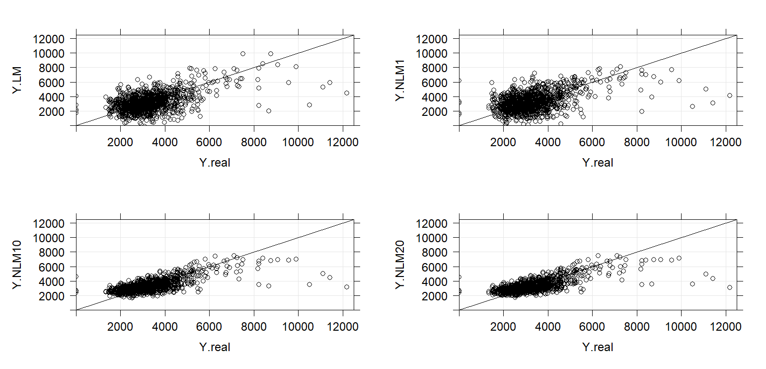
Figure 1: One realization of a model versus real values

In Figure 1 we can compare the distribution of the real population values of the variable of interest (Y.real on OX axis) and one realization of the variable of interest generated from: model LM given by (24) (Y.LM on OY axis), model NLM1 given by (25) (Y.NLM1 on OY axis), model NLM10 given by (26) with $a=10$ (Y.NLM10 on OY axis), model NLM20 given by (26) with $a=20$ (Y.NLM20 on OY axis). The scatter plots are similar because fixed effects in all models are assumed to be equal to estimates based on the population real dataset.

5.2 Simulation study of properties of predictors

In the simulation study of accuracy of predictors, the number of Monte Carlo iterations is set to be equal $K=2000$. We study four plug-in predictors given by general formula (3):

• of the subpopulation mean based on the LMM (24) fitted to the data (in figures denoted by LMM mean),

• of the subpopulation mean based on the GB (GB mean),

• of the subpopulation median based on the LMM (24)(LMM median),

• of the subpopulation median based on the GB (GB median).

The GB tree algorithm in the simulation study is performed with xgboost R library.

In the Figure 2 we present the following relative measures allowing for the accuracy assessment of the predictors:

• the relative prediction bias

  $${rB}^{(sym)}\left(\hat{\theta}\right)=\frac{\frac{1}{K}\sum_{k=1}^{K}{{(\hat{\theta}}^{(k)}-\theta^{(k)})}}{\frac{1}{K}\sum_{k=1}^{K}\theta^{(k)}}100,$$ (27)

• the prediction relative RMSE (rRMSE)

  $${rRMSE}^{\left(sym\right)}\left(\hat{\theta}\right)=\frac{\sqrt{\frac{1}{K}\sum_{k=1}^{K}\left({\hat{\theta}}^{(k)}-\theta^{(k)}\right)^{2}}}{\frac{1}{K}\sum_{k=1}^{K}\theta^{(k)}}100.$$ (28)

In Figure 3 we present the computed values of absolute prediction measures:

• the RMSE

  $${RMSE}^{\left(sym\right)}\left(\hat{\theta}\right)={\sqrt{\frac{1}{K}\sum_{k=1}^{K}\left({\hat{\theta}}^{(k)}-\theta^{(k)}\right)^{2}}},$$ (29)

• the quantile of absolute prediction error (QAPE) of order $p$

  $${QAPE}_{p}(\hat{\theta})=q_{p}(|{\hat{\theta}}^{(1)}-\theta^{(1)}|,\dots,|{\hat{\theta}}^{(k)}-\theta^{(k)}|,\dots,|{\hat{\theta}}^{(K)}-\theta^{(K)}|).$$ (30)

  where $q_{p}(.)$ is the $p$th quantile.

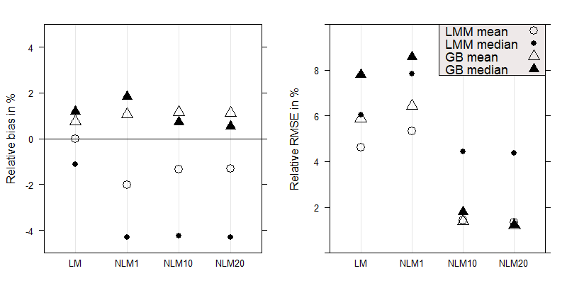
Figure 2: Relative biases and relative RMSEs (in %) of predictors

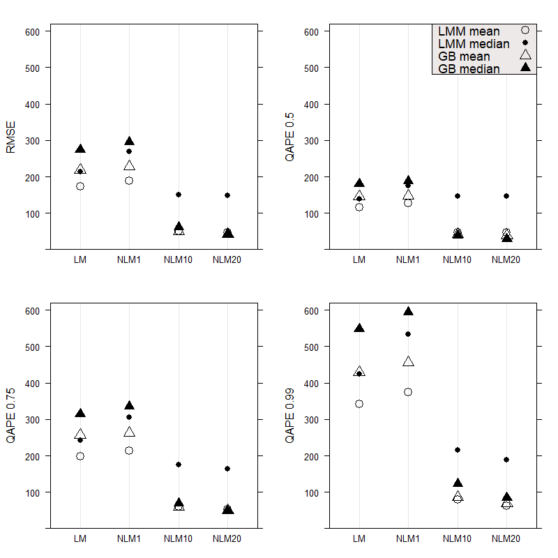
Figure 3: RMSEs and QAPEs of predictors

Firstly, let us consider the results under the correctly specified model where the mean is predicted, which means that the values of the variable of interest are generated based on LM model and the same model is used to construct LMM mean predictor, which is the EBLUP in this case. It means it is the empirical (estimated) version of the optimal predictor, in the sense that the predictor minimizes the prediction MSE in the class of the unbiased predictors. We can see these theoretical properties in our simulation results. The relative simulation biases presented on the left part of Figure 2 of the LMM mean EBLUP predictor (denoted by "$\circ$" symbol) under LM are very close to zero, and – see the right part of Figure 2 – the rRMSE of the predictor is smaller, under LM model, comparing with another mean predictor – GB mean (denoted by "$\triangle$" symbol). Similarly, in Figure 3, values of all considered accuracy measures for LMM mean predictor are smaller comparing with GB mean under LM model. To sum up, although LMM mean predictor is optimal in the discussed sense, the GB mean predictor is only slightly less accurate in this case.

Secondly, let us consider the results under the correctly specified LM model where the median is predicted. In this case, LMM median predictor is not EBLUP. The absolute values of the relative biases of LMM median (denoted by "$\bullet$" symbol) and GB median (denoted by "$\blacktriangle$" symbol) presented in the left part of Figure 2 are similar (but their biases have opposite signs). The values of all considered accuracy measures presented in the right part of the Figure 2 and in Figure 3 are smaller for LMM median predictor comparing with GB median, but – as it was observed for the case, where the mean is predicted – only slightly.

Thirdly, the problem of model misspecification is studied. Under models NLM1, NLM10 and NLM20, the absolute biases of the proposed GB-based predictors are smaller than the respective absolute biases of the LMM-based predictors (see the left part of Figure 2). As shown on the right part of Figure 2 and in Figure 3, under model NLM1, even though the model is misspecified, the accuracy of LMM-based predictors is still slightly better than the accuracy of GB-based predictors. However, under NLM10 and NLM20 the accuracy of GB-based predictor of the mean measured by the RMSE (and rRMSE) and QAPEs of orders 0.5 and 0.75 is better by up to 15% (if measured by QAPE of order 0.5 for NLM20), and in the case of QAPE of order 0.99 – very similar. For the same models, GB-based predictor of the median is from 1.75 to 5.25 times more accurate comparing with the LMM-based predictor of the median, where the results depend on the accuracy measure.

Summing up, we have shown that the GB-based predictors are very good alternatives to the LMM-based predictors (including optimal predictors), giving only slightly less accurate results under the correctly specified LMM, and better results even for small departures from the assumed models. Hence, having a new predictor with good properties, the next step is essential. The step without which, it is not possible to use the proposed predictor appropriately in practice. It is the ability to compare the accuracy of the predictor with its competitors properly based on sample data. It means that the proposed estimators of accuracy measures of the proposed predictor should have very good properties which are similar comparing with estimators of accuracy measures of the competitive predictors.

5.3 Simulation study of properties of accuracy measures estimators

In this simulation study, the properties of RMSE and QAPE estimators are analysed. The assumed number of Monte Carlo iterations is $K=1000$; the number of the parametric, residual and the first level of double bootstrap iterations equals $B=200$; and the number of the double bootstrap second level iterations is assumed to be $C=1$. The assumed value of $C$ is set due to the time-consuming computations but it is shown to be the best choice in the case of the EBP (see Erciulescu and Fuller,, 2014). Although the considered PLUG-IN predictor is similar to the EBP, in further research other values of $C$ can be considered as well, especially if the double bootstrap procedure will occur to be the preferable method based on the results of the conducted simulation analysis.

We study the properties of RMSE estimators based on:

• parametric bootstrap, given by (7) (denoted below by param),

• residual bootstrap with and without the correction, given by (7), where parametric bootstrap prediction errors are replaced by appropriate residual bootstrap prediction errors (rbCor and rb),

• double bootstrap, given by (13), (15), (17) with $C=1$, (18), and (19) (denoted by db1, dbTel, db1HM, db1EF, and dbTelEF, respectively),

and QAPE estimators based on:

• parametric bootstrap, given by (8) (param),

• residual bootstrap with and without the correction, given by (8), where parametric bootstrap prediction errors are replaced by appropriate residual bootstrap prediction errors (rb and rbCor),

• double bootstrap, given by (22) and (23) (db1 and dbTel).

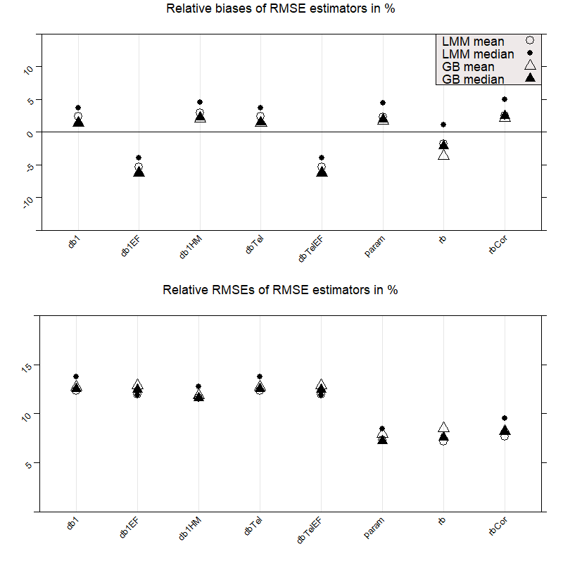
Figure 4: Relative biases and relative RMSEs (in %) of RMSE estimators

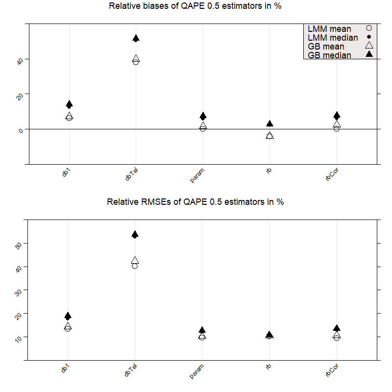
Figure 5: Relative biases and relative RMSEs (in %) of QAPE(0.5) estimators

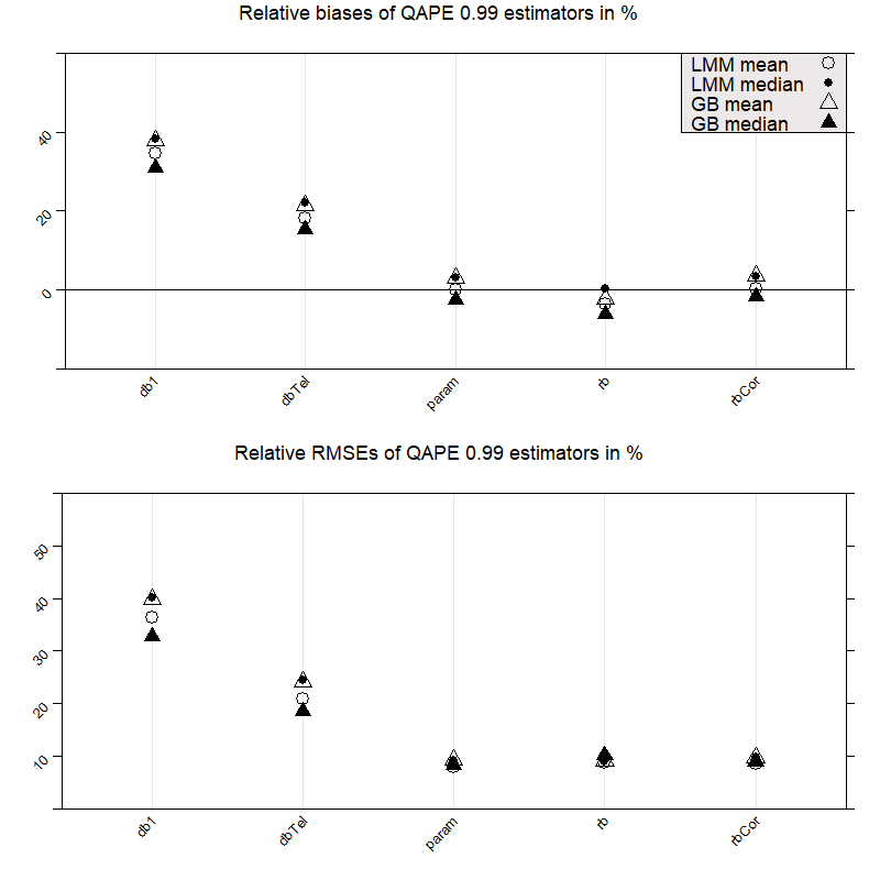
Figure 6: Relative biases and relative RMSEs (in %) of QAPE(0.99) estimators

We present values of their relative biases and relative RMSEs. They are computed based on (27) and (28), respectively, where $\hat{\theta}^{(k)}$ are replaced by the values of the bootstrap RMSE estimators (or bootstrap QAPE estimators) obtained in the $k$th iteration of the simulation study, and ${\theta}^{(k)}$ are replaced by the RMSE given by the square of (29) (or by the QAPE given by (30)).

Firstly, let us analyse the biases of RMSE estimators presented in the top part of Figure 4 and of QAPE estimators presented in the top parts of Figures 5 and 6. For all the considered cases, both for GB-based and LMM-based predictors, the parametric and residual (with and without correction) bootstrap algorithms lead to only slightly biased RMSE and QAPE estimators, while the results for various double bootstrap estimators are not conclusive. Secondly, the accuracy of RMSE estimators presented in the bottom part of Figure 4 and of QAPE estimators presented in the bottom parts of Figure 5 and 6 is analysed. In this case, the smallest values of relative RMSEs are observed if the parametric and both residual bootstrap algorithms are used - relative RMSEs do not exceed: for RMSE estimators $10\%$, for QAPE(0.5) estimators $14\%$, and for QAPE(0.99) estimators $11\%$.

Summing up, for each of the considered bootstrap algorithms the properties of a certain RMSE or QAPE estimator are very similar irrespective of the predictor (GB-based or LM-based) and the prediction problem (the prediction of the mean or the median). What is more, RMSE and QAPE estimators based on three bootstrap algorithms, namely the parametric and two residual bootstrap methods, have very good properties. It means that using them, we can accurately estimate the accuracy of the proposed predictor and reliably compare it with the estimated accuracy of different predictors. This, in our opinion, paves the way for the possibility of practical use of the proposed predictor in practice, where it is important not only to be able to assess the population or subpopulation characteristics, but also to estimate the prediction accuracy and to compare the prediction accuracy estimates.

6 Conclusion

We proposed a gradient-boosting based predictor of any population or subpopulation characteristic. We showed the under the LMM the accuracy of the proposed predictor is similar to the accuracy of the plug-in predictor based on the LMM, but it is better regarding even relatively small departures from the linearity. Therefore, we lose little under the correctly specified model, and we can gain a lot (we obtained up to 5.25 times more accurate results) under an even slightly misspecified model.

What is more, the properties of all studied accuracy measures estimators under the LMM are very similar for both predictors. Hence, in practice, we can compare estimators of accuracy measures of the proposed predictor and classic predictors based on the LMM. Finally, we showed very good properties of the parametric and residual bootstrap RMSE and QAPE estimators, which allows us to recommend them for empirical research.

Appendix A. Parametric and residual bootstrap procedures

The parametric bootstrap procedure is implemented according to González-Manteiga et al., (2007) and González-Manteiga et al., (2008) and could be described in the following steps.

1. Based on $n_{(L)}$ sample observations of the dependent and independent variables, model parameters are estimated.

2. Based on $N_{(L)}$ population observations of the independent variables, a realization of the population vector of the dependent variable of size $N_{(L)}\times 1$ is generated under (2), where parameters are replaced by their estimates (e.g. Restricted Maximum Likelihood estimates) and under normality of random effects and random components.

3. The population vector of the dependent variable generated in the previous step is decomposed into two subvectors: the first of size $n_{(L)}\times 1$ for the sample observations, and the second of size $(N_{(L)}-n_{(L)})\times 1$ for non-sampled observations.

4. Based on the generated population vector of the dependent variable, the bootstrap realization of the predicted characteristic, denoted for the $b$th iteration by $\theta^{*(b)}$, is computed.

5. The generated sample vector of the dependent variable is used to compute the vector of estimates of model parameters, and based on these vectors, the bootstrap realization of the predictor $\hat{\theta}$, denoted for the $b$th iteration by $\hat{\theta}^{*(b)}$, is computed.

6. The bootstrap realization of the prediction error is calculated as

   $$u^{*(b)}=\hat{\theta}^{*(b)}-\theta^{*(b)}.$$

7. Steps (b)-(f) are repeated $B$ times.

The detailed description of the algorithm can be found in Carpenter et al., (2003), Chambers and Chandra, (2013), and Thai et al., (2013). To obtain the residual bootstrap procedure, the step (b) in the parametric bootstrap algorithm presented above should be replaced with:

1. Based $N_{(L)}$ on population observations of the independent variables, estimated fixed effects, and simple random samples with replacement of predicted random effects and estimated random components, a realization of the population vector of the dependent variable of size $N_{(L)}\times 1$ is generated under (2).

If the model covers more than one vector of random effect at the same level of grouping, then the predicted values of these effects for the same level are sampled jointly (rows of the matrix formed by these vectors are sampled with replacement). The residual bootstrap algorithm can also be performed with a so-called “correction procedure” (Thai et al.,, 2013, p. 132) to improve the properties of the residual bootstrap estimators due to the underdispersion of the uncorrected residual bootstrap distributions.

Appendix B. Double bootstrap procedure

As presented by Hall and Maiti, (2006), Erciulescu and Fuller, (2014), Pfeffermann et al., (2013), the double bootstrap procedure consists of two parametric bootstrap levels. For the $b$th iteration of the first level, the following second level is conducted.

In the $c$th iteration ($c=1,2,...,C$) of the second level:

1. Based on $n_{(L)}$ sample observations of the dependent variable generated at the first level and independent variables, model parameters are estimated.

2. Based on $N_{(L)}$ population observations of the independent variables, a realization of the population vector of the dependent variable of size $N_{(L)}\times 1$ is generated under (2) where parameters are replaced by their estimates (obtained in the previous step of the second level bootstrap procedure) and under normality of random effects and random components.

3. The population vector of the dependent variable generated in the previous step is decomposed into two subvectors: the first of size $n_{(L)}\times 1$ for the sample observations, and the second of size $(N_{(L)}-n_{(L)})\times 1$ for non-sampled observations.

4. Based on the generated (at the second level bootstrap procedure) population vector of the dependent variable, the bootstrap realization of the predicted characteristic, denoted by $\theta^{**(b,c)}$, is computed.

5. The generated (at the second level bootstrap procedure) sample vector of the dependent variable is used to compute the vector of estimates of model parameters, and based on these vectors, the bootstrap realization of the predictor $\hat{\theta}$, denoted by $\hat{\theta}^{**(b,c)}$, is computed.

6. The second-level bootstrap prediction error is computed as

   $$u^{**(b,c)}=\hat{\theta}^{**(b,c)}-\theta^{**(b,c)}.$$

7. Steps (b)-(f) are repeated $C$ times.

References

- Ashofteh and Bravo, (2021) Ashofteh, A. and Bravo, J. M. (2021). "Data science training for official statistics: A new scientific paradigm of information and knowledge development in national statistical systems". Statistical Journal of the IAOS, 37(3):771–789. Publisher: IOS Press.
- Beck et al., (2018) Beck, M., Dumpert, F., and Feuerhake, J. (2018). Machine learning in official statistics. arXiv preprint arXiv:1812.10422.
- Breiman, (2001) Breiman, L. (2001). "Statistical Modeling: The Two Cultures (with comments and a rejoinder by the author)". Statistical Science, 16(3).
- Breiman et al., (1984) Breiman, L., Friedman, J., Stone, C. J., and Olshen, R. A. (1984). Classification and Regression Trees. Taylor & Francis.
- Carpenter et al., (2003) Carpenter, J. R., Goldstein, H., and Rasbash, J. (2003). "A novel bootstrap procedure for assessing the relationship between class size and achievement". Journal of the Royal Statistical Society: Series C (Applied Statistics), 52(4):431–443.
- Chambers and Chandra, (2013) Chambers, R. and Chandra, H. (2013). "A Random Effect Block Bootstrap for Clustered Data". Journal of Computational and Graphical Statistics, 22(2):452–470.
- Chandra et al., (2012) Chandra, H., Salvati, N., Chambers, R., and Tzavidis, N. (2012). "Small area estimation under spatial nonstationarity". Computational Statistics & Data Analysis, 56.
- Chen et al., (2019) Chen, J., de Hoogh, K., Gulliver, J., Hoffmann, B., Hertel, O., Ketzel, M., Bauwelinck, M., van Donkelaar, A., Hvidtfeldt, U. A., Katsouyanni, K., Janssen, N. A. H., Martin, R. V., Samoli, E., Schwartz, P. E., Stafoggia, M., Bellander, T., Strak, M., Wolf, K., Vienneau, D., Vermeulen, R., Brunekreef, B., and Hoek, G. (2019). "A comparison of linear regression, regularization, and machine learning algorithms to develop Europe-wide spatial models of fine particles and nitrogen dioxide". Environment International, 130:104934.
- Chwila and Żądło, (2022) Chwila, A. and Żądło, T. (2022). "On properties of empirical best predictors". Communications in Statistics - Simulation and Computation, 51(1):220–253.
- Corral et al., (2022) Corral, P., Molina, I., Cojocaru, A., and Segovia, S. (2022). "Guidelines to Small Area Estimation for Poverty Mapping". World Bank.
- Dagdoug et al., (2023) Dagdoug, M., Goga, C., and Haziza, D. (2023). "Model-Assisted Estimation Through Random Forests in Finite Population Sampling". Journal of the American Statistical Association, 118(542):1234–1251.
- Davidson and MacKinnon, (2007) Davidson, R. and MacKinnon, J. G. (2007). "Improving the reliability of bootstrap tests with the fast double bootstrap". Computational Statistics & Data Analysis, 51(7):3259–3281.
- De Broe et al., (2020) De Broe, S., Struijs, P., Daas, P., van Delden, A., Burger, J., van den Brakel, J., ten Bosch, O., Zeelenberg, K., and Ypma, W. (2020). "Updating the paradigm of official statistics: New quality criteria for integrating new data and methods in official statistics". Working paper 02-20, Center for Big Data Statistics, Statistics Netherlands, The Hague.
- Deville and Särndal, (1992) Deville, J.-C. and Särndal, C.-E. (1992). "Calibration Estimators in Survey Sampling". Journal of the American Statistical Association, 87(418):376–382.