Gravitational Lensing and Clues of $r_{d}$ and $H_{0}$ Tension: Viscous Modified Chaplygin Gas and Variable Modified Chaplygin Gas in Loop Quantum Cosmology

Abstract

This paper investigates the accelerated cosmic expansion in the late Universe by examining two dark energy models, namely viscous modified Chaplygin gas (VsMCG) and variable modified Chaplygin gas (VMCG), within the framework of loop quantum cosmology alongside the $\Lambda$CDM model. Our main objective is to constrain fundamental cosmic parameters in these dark energy models with $\Lambda$CDM model using 30 of the latest $H(z)$ measurements obtained from the cosmic chronometers method (CC), including Type Ia Supernovae, Gamma-Ray Bursts (GRB), Quasars, and 24 uncorrelated baryon acoustic oscillations (BAO) measurements from recent galaxy surveys across a redshift range from $0.106<z<2.33$. Additionally, we include the most recent Hubble constant measurement from Riess in 2022 to further enhance our constraints on fundamental cosmic parameters. In the $\Lambda$CDM, VsMCG, and VMCG frameworks, Our investigation yields best-fit parameters for the Hubble parameter ($H_{0}$) and sound horizon ($r_{d}$). The outcomes underscore a significant disparity between ($H_{0}$) and $r_{d}$) values using late-time observational measurements, reflecting the widely recognized $H_{0}$ and $r_{d}$ tensions. Further, we study the gravitational lensing optical depth of the two dark energy models by plotting $\tau(z_{s})/F$ vs $z_{s}$ graphs. The probability of finding gravitational lenses (optical depth) in both our models increases with source redshift $z_{s}$. The change in optical depth behaviour for different sets of parameter value constraints through data sets is also graphically analysed. Joint analysis of VsMCG and VMCG with standard cosmological model $\Lambda$CDM is also carried out to study the optical depth behaviour. While the three models diverge in the early Universe, but for low redshift, they are found to be indistinguishable from each other. Finally, by employing the Akaike information criteria approach for model comparison, our analysis indicates that none of the two dark energy models can be dismissed based on the latest observational measurements.

I Introduction

Our universe is undergoing accelerated expansion, a phenomenon supported by multiple independent studies [1, 2, 3, 4] conducted over the past two decades. While the actual cause of this accelerated phenomenon is still debatable, many attribute it to huge negative pressure build-up in our present Universe. Many assume that some kind of ‘mysterious’ energy must be at play here and have named it ‘dark energy’ (DE, hereafter). Dark energy, or DE, almost occupies $70\%$ of our Universe, so its study has been of immense importance. Over the years, researchers have proposed numerous such DE candidates to explain our accelerating Universe, and among them, the cosmological constant $\Lambda$ happens to be the simplest. The other candidates includes Chaplygin gas [5, 6], quintessence [7, 8], phantom energy [9], holographic dark energy [10, 11], among the numerous others in literature [12]. Despite the diverse range of proposed dark energy candidates, the key to unravelling the mysteries of dark energy lies not only in theoretical constructs but also in empirical observations. Observational cosmology has thus become instrumental in discerning the nature of dark energy. Among the observational probes employed by cosmologists, the study of the large-scale structure of the Universe stands out prominently. Observations of the large-scale structure, which include the spatial distribution of galaxies, galaxy clusters, and cosmic voids, offer invaluable insights into the underlying dynamics of cosmic evolution [13]. By scrutinizing the cosmic web on vast scales, cosmologists can glean crucial information about the composition of the Universe, its expansion history, and the influence of dark energy on cosmic structures [14]. However, as observational techniques have advanced, they have revealed a perplexing tension between early-time and late-time cosmological observations. This tension manifests in discrepancies between measurements obtained from the early Universe, such as those derived from the cosmic microwave background (CMB) radiation [15] and those obtained from more recent observations of the local Universe, such as those from Type Ia supernovae [16] and Baryon Acoustic Oscillations (BAO). BAO plays a pivotal role, offering a unique and powerful tool for understanding the large-scale structure of the Universe. These oscillations are imprints left on the distribution of matter in the early Universe, originating from the coupled interaction between photons and baryons (protons and neutrons) before the era of recombination [17]. The significance of BAO lies in their ability to serve as standard rulers on cosmological scales. As the Universe expands, these primordial density fluctuations lead to characteristic patterns in the distribution of galaxies and cosmic microwave background radiation. The formation of BAO can be traced back to the sound waves that propagated through the primordial plasma of the early Universe. As the Universe expanded, the sound waves left behind a distinctive pattern of overdense and underdense regions, creating a preferred scale known as the BAO scale or sound horizon [18]. This scale acts as a standard ruler, allowing cosmologists to measure the geometry and expansion rate of the Universe over cosmic time. The BAO scale, or sound horizon, serves as a crucial cosmological standard because its size is determined by fundamental cosmological parameters, such as the density of baryons and dark matter, as well as the speed of sound in the primordial plasma. Observations of BAO in the large-scale distribution of galaxies provide a powerful constraint on these parameters and offer insights into the nature of dark energy [19]. In the field of cosmology, the study of BAO and the sound horizon has become an essential tool for precision cosmological measurements. Large galaxy surveys, such as the Sloan Digital Sky Survey (SDSS), have played a key role in mapping the distribution of galaxies and detecting the BAO signal [20]. By analyzing the BAO scale in the clustering of galaxies, researchers can infer the expansion history of the Universe and shed light on the mysterious components of dark matter and dark energy. Thus, Baryon Acoustic Oscillations stand as a cornerstone in our quest to unravel the fundamental properties and evolution of the cosmos.

While BAO provide valuable insights about the large-scale structure of the Universe and the behavior of dark energy, the accelerating expansion of the cosmos remains a profound puzzle that has spurred researchers to explore alternative explanations. Many assume that Einstein’s gravitational theory might be incomplete. So, researchers modified the underlying gravity theory (and hence, the name modified theory of gravity [21, 22]) to incorporate the accelerating phase of our Universe. While these theories effectively explain the formation of structures and gravitational interactions on a large scale, quantum gravity becomes necessary to understand behaviors at smaller scales. Further, the backward evolution of our Universe in time results in the collapse of our Universe into a single point with diverging energy density. Such instances lead to the failure of our classical gravity theory, rendering it ineffective in describing the unfolding events. Quantum gravity, with its distinct dynamics on smaller scales, is expected to solve this dilemma. One such theory based upon quantum gravity is loop quantum cosmology (LQC, hereafter) [23, 24]. In recent years, several DE models have been studied in its framework. Jamil et al. [25] investigated the combination of modified Chaplygin gas with dark matter within the LQC framework, resolving the cosmic coincidence problem. The authors in ref. [26], discovered that loop quantum effects could prevent future singularities in the FRW cosmology. Given its importance, in our present study as well, we considered two models of Chaplygin gas, namely, viscous modified Chaplygin gas (VsMCG) and variable modified Chaplygin gas (VMCG) in LQC framework, to analyze their optical depth behaviour by constraining the model parameters to their best-fit values. Further, the significance of the study of gravitational lensing also has long been recognised in cosmology, and the phenomenal work of Refsdal et al. [27] in this context is worth mentioning. Over recent years, gravitational lensing emerged as an important tool for studying dark matter, dark energy, and black holes, among many others. Gravitational lensing optical depth represents the likelihood of the formation of multiple images owing to the influence of gravitational lenses in our Universe. It was first used by ref. [28, 29] and consequently by many others [30, 31, 32], including Kundu et al. [33] to study and understand dark energy models. Our present paper uses this lensing phenomenon to qualitatively analyse the two DE models against their constraint parameter values and record the changes graphically. This methodology of studying the gravitational lensing optical depth of DE models can give us an estimation in understanding the large-scale structure of our Universe, thereby helping us better understand our models.

Finally, our paper is organized as follows: Section II delves into the background equations of the two dark energy models within the framework of loop quantum cosmology. Section III outlines the methodology employed to constrain the parameters of the dark energy models using various datasets. Section IV is dedicated to the study of the lensing phenomenon, including the derivation of the equation for optical depth to be used in our study. In Section V, we present the outcomes of our study, and we conclude by discussing our findings in Section VI.

II Background equations: Loop Quantum Cosmology

In loop quantum cosmology, for a isotropic and homogeneous Universe the background equations are defined by:

$$H^{2}=\frac{1}{3}\left(1-\frac{\rho}{\rho_{1}}\right)\rho,$$ (1)

$$\dot{H}=-\frac{1}{2}\left(1-\frac{2\rho}{\rho_{1}}\right)(\rho+p)$$ (2)

where $\rho_{1}=\frac{\sqrt{3}}{16\pi^{2}\gamma^{3}G^{2}\hbar}$ is the critical loop quantum density and $\gamma$ the dimensionless “Barbero-Immirzi parameter”. The conservation equation in LQC is given by:

$$\dot{\rho}+3H(\rho+p)=0$$ (3)

Assuming the matter content of our Universe to be a combination of DM and DE, the quantities $\rho$ and $p$ defined in Eqs (1) and (2) will modify to $\rho=\rho_{m}+\rho_{d}$ and $p=p_{m}+p_{d}$. With the consideration that both DM and DE are separately conserved, the equation (3) now seperates into two distinct equations as follows:

$$\dot{\rho}_{m}+3H(\rho_{m}+p_{m})=0,$$ (4)

$$\dot{\rho}_{d}+3H(\rho_{d}+p_{d})=0,$$ (5)

Since, pressure in dark matter is very negligible (i.e. $p_{m}=0$), equation (4) gives $\rho_{m}=\rho_{m0}(1+z)^{3}$. Here, $\rho_{m0}$ represent the density value at the present epoch.

II.1 Viscous modified Chaplygin gas (VsMCG)

The expression for pressure in the case of viscous modified Chaplygin gas (VsMCG) is given by [34]:

$$p_{d}=A\rho_{d}-\frac{B}{\rho_{d}^{\alpha}}-3\zeta_{0}\sqrt{\rho_{d}}H$$ (6)

where $A$, $B$ and $\alpha$ are constants. Substituting $p_{d}$ from Eq (6) in Eq (5), we get:

$$\rho_{d}=\left(\frac{B}{1+A-\sqrt{3}\zeta_{0}}+\frac{C_{1}}{a^{3(1+\alpha)(1+A-\sqrt{3}\zeta_{0})}}\right)^{\frac{1}{1+\alpha}}$$ (7)

where $C_{1}$ is an integrating constant. The above expression can be further re-written as:

$$\rho_{d}=\rho_{d0}\{A_{s}+(1-A_{s})(1+z)^{3(1+\alpha)(1+A-\sqrt{3}\zeta_{0})}\}^{\frac{1}{1+\alpha}}$$ (8)

where $\rho_{d0}$ being the DE density value at the present epoch, $A_{s}=\frac{B}{(1+A-\sqrt{3}\zeta_{0})C_{1}+B}$ satisfying the conditions $0<A_{s}<1$ and $1+A-\sqrt{3}\zeta_{0}>0$, and $\rho_{d0}^{1+\alpha}=\frac{(1+A-\sqrt{3}\zeta_{0})C_{1}+B}{1+A-\sqrt{3}\zeta_{0}}$. Thus, we can write the Hubble parameter from equation (1) as follows:

$$H^{2}(z)=H_{0}^{2}\bigg{[}\Omega_{m0}(1+z)^{3}+\Omega_{d0}\Big{\{}A_{s}+(1-A_{s})(1+z)^{3(1+\alpha)(1+A-\sqrt{3}\zeta_{0})}\Big{\}}^{\frac{1}{1+\alpha}}\bigg{]}\times\\ \bigg{[}1-\frac{3H_{0}^{2}}{\rho_{1}}\Big{\{}\Omega_{m0}(1+z)^{3}+\Omega_{d0}\Big{\{}A_{s}+(1-A_{s})(1+z)^{3(1+\alpha)(1+A-\sqrt{3}\zeta_{0})}\Big{\}}^{\frac{1}{1+\alpha}}\Big{\}}\bigg{]}$$ (9)

where $\Omega_{m0}=\frac{\rho_{m0}}{3H_{0}^{2}}$ and $\Omega_{d0}=\frac{\rho_{d0}}{3H_{0}^{2}}$ are the dimensionless parameters all defined at the present epoch. Further, substituting $z=0$ in equation (9) and equating the RHS to ‘$1$’ we get:

$$\Big{[}\Omega_{m0}+\Omega_{d0}\Big{]}\times\bigg{[}1-\frac{3H_{0}^{2}}{\rho_{1}}\Big{\{}\Omega_{m0}+\Omega_{d0}\Big{\}}\bigg{]}=1$$ (10)

which simplifies to

$$\Omega_{d0}=\frac{1}{6H_{0}^{2}}\left(\rho_{1}+\sqrt{\rho_{1}^{2}-12\rho_{1}H_{0}^{2}}\right)-\Omega_{m0}$$ (11)

II.2 Variable modified Chaplygin gas (VMCG)

The expression for pressure in the case of variable modified Chaplygin gas (VMCG) is given by [35]:

$$p_{d}=C\rho_{d}-\frac{D(a)}{\rho_{d}^{\beta}}$$ (12)

where $0\leq\beta\leq 1$ and $C>0$. Assuming, $D(a)=D_{0}a^{-n}$ where $D_{0}>0$ and $n>0$, we get from Eq (5):

$$\rho_{d}=\left[\frac{3(1+\beta)D_{0}}{\{3(1+\beta)(1+C)-n\}a^{n}}+\frac{K}{a^{3(1+C)(1+\beta)}}\right]^{\frac{1}{1+\beta}}$$ (13)

where $K(>0)$ is an arbitrary integrating constant and $3(1+\beta)(1+C)-n>0$. Also, here $n$ must be positive, or else for $a\rightarrow\infty$ we would have $\rho_{d}\rightarrow\infty$ thereby contradicting our case for expanding Universe. The expression for $\rho_{d}$ above can be further simplified to:

$$\rho_{d}=\rho_{d0}\left[\frac{C_{s}}{a^{n}}+\frac{1-C_{s}}{a^{3(1+C)(1+\beta)}}\right]^{\frac{1}{1+\beta}}$$ (14)

where $\rho_{d0}$ denotes the DE density value at the present epoch, $C_{s}=1-\frac{K}{\rho_{d0}^{1+\beta}}$ and $\rho_{d0}^{1+\beta}=K+\frac{3(1+\beta)D_{0}}{3(1+\beta)(1+C)-n}$. Thus, we can write the Hubble parameter from equation (1) as follows:

$$H^{2}(z)=H_{0}^{2}\bigg{[}\Omega_{m0}(1+z)^{3}+\Omega_{d0}\Big{\{}C_{s}(1+z)^{n}+(1-C_{s})(1+z)^{3(1+C)(1+\beta)}\Big{\}}^{\frac{1}{1+\beta}}\bigg{]}\times\\ \bigg{[}1-\frac{3H_{0}^{2}}{\rho_{1}}\Big{\{}\Omega_{m0}(1+z)^{3}+\Omega_{d0}\Big{\{}C_{s}(1+z)^{n}+(1-C_{s})(1+z)^{3(1+C)(1+\beta)}\Big{\}}^{\frac{1}{1+\beta}}\Big{\}}\bigg{]}$$ (15)

where $\Omega_{d0}$ is given in (11).

III Methodology

In our study, we carefully picked a specific set of recent Baryon Acoustic Oscillation (BAO) measurements from various galaxy surveys, with the primary contributions coming from observations made by the Sloan Digital Sky Survey (SDSS) [36, 37, 38, 39, 40, 41]. We also included valuable data from the Dark Energy Survey (DES) [42], the Dark Energy Camera Legacy Survey (DECaLS) [43], and 6dFGS BAO [44] to enhance the diversity of our dataset. Recognizing the potential for correlations among selected data points, we took steps to address this issue. While we intentionally crafted a subset to minimize highly correlated points, acknowledging and dealing with possible correlations within our chosen data points was deemed crucial. For a robust estimation of systematic errors, we used mocks generated from N-body simulations to accurately determine covariance matrices. Given the diverse nature of measurements from various observational surveys, obtaining precise covariance matrices between them posed a significant challenge. To address this, we adopted the covariance analysis approach outlined in [45], specifically using $C_{ii}=\sigma_{i}^{2}$. To simulate correlations within our chosen subsample, we introduced non-diagonal elements into the covariance matrix while maintaining symmetry. Incorporating non-negative correlations involved randomly selecting up to 12 pairs of data points and assigning non-diagonal elements with magnitudes of $C_{ij}=0.5\sigma_{i}\sigma_{j}$. Here, $\sigma_{i}$ and $\sigma_{j}$ denote the 1$\sigma$ errors of data points $i$ and $j$. This approach allowed us to effectively represent correlations within 55% of our chosen BAO dataset. The variation of some cosmological parameters of $\Lambda$CDM according to the number of correlated pairs is shown in Table 1. Fig. 1 displays the posterior distributions for the $\Lambda$CDM Model with and without the incorporation of a test random covariance matrix comprising fourteen components. The influence of this covariance matrix, ranging from null to fourteen components, appears negligible, closely resembling the uncorrelated dataset. Moving on to determining the best-fit values for our cosmological model parameters, we expanded the BAO dataset by incorporating thirty uncorrelated Hubble parameter measurements obtained through the cosmic chronometers (CC) method discussed in [46, 47, 48, 49]. Additionally, we included the latest Pantheon sample data on Type Ia Supernovae [50]. To broaden our observational scope further, we introduced 24 binned quasar distance modulus data from [51], a set of 162 Gamma-Ray Bursts (GRBs) as outlined in [52], and the recent Hubble constant measurement (R22) [53] as an additional prior. In our analysis, we used a nested sampling approach implemented in the open-source Polychord package [54], complemented by the GetDist package [55] to present our results in a clear and informative manner.

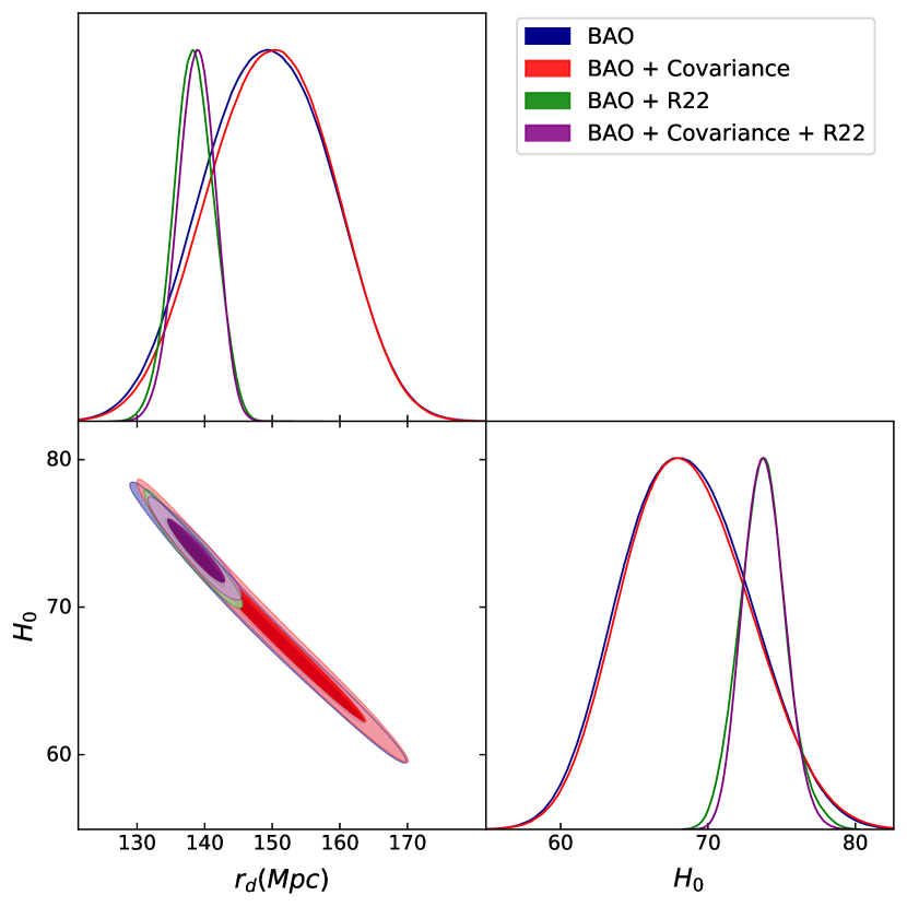
(a) $r_{d}$ vs $H_{0}$

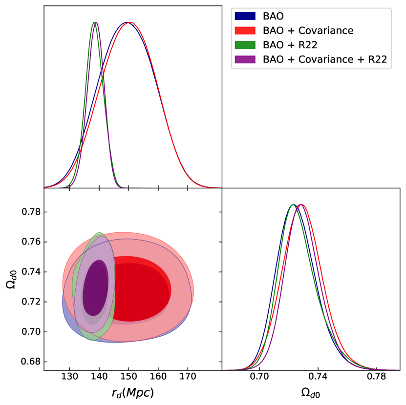
(b) $r_{d}$ vs $\Omega_{d0}$

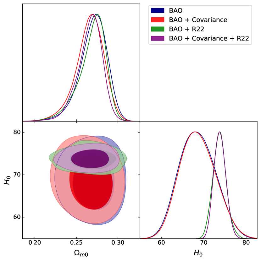
(c) $H_{0}$ vs $\Omega_{d0}$

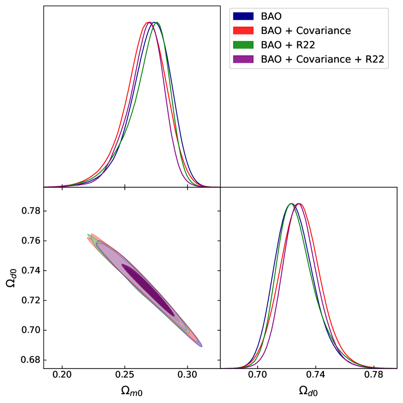
(d) $\Omega_{m0}$ vs $\Omega_{d0}$

Figure 1: Comparison of posterior distributions in $\Lambda$CDM with and without a randomly tested covariance matrix of fourteen components shows negligible impact. This renders the dataset nearly indistinguishable from an uncorrelated one. Covariance matrices beyond fourteen components exhibit minimal influence.

Parameters	$n$ correlated pairs	BAO	BAO+R22
$\Omega_{m0}$	n = 0	$0.270\pm 0.015$	$0.266\pm 0.015$
$\Omega_{\Lambda 0}$		$0.725\pm 0.011$	$0.728\pm 0.0125$
$\Omega_{m0}$	n = 7	$0.264\pm 0.016$	$0.261\pm 0.015$
$\Omega_{\Lambda 0}$		$0.730\pm 0.013$	$0.733\pm 0.011$
$\Omega_{m0}$	n = 14	$0.266\pm 0.015$	$0.264\pm 0.016$
$\Omega_{\Lambda 0}$		$0.728\pm 0.011$	$0.730\pm 0.012$

Table 1: The table shows slight variations in different cosmological parameters when comparing scenarios with uncorrelated pairs ($n=0$) to those with $n=7$ and $n=14$ randomly introduced correlated pairs.

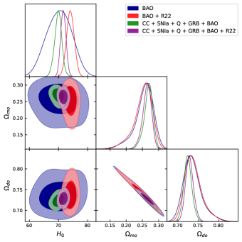
Figure 2: The figure illustrates 1$\sigma$ and 2$\sigma$ regions using the standard $\Lambda$CDM model to demonstrate the posterior distribution of various observational data measurements.

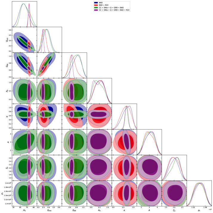
Figure 3: The figure illustrates the posterior distribution of various observational data measurements using the Viscous Modified Chaplygin Gas model, highlighting the 1$\sigma$ and 2$\sigma$ regions.

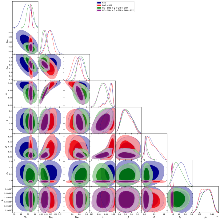
Figure 4: The figure illustrates the posterior distribution of various observational data measurements using the Variable Modified Chaplygin Gas model, highlighting the 1$\sigma$ and 2$\sigma$ regions.

MCMC Results
Model	Parameters	Priors	BAO	BA0 + R22	CC + SC + BAO	CC + SC + BAO + R22
	$H_{0}$	[50,100]	$69.089209_{\pm 4.396874}^{\pm 6.252595}$	$73.906596_{\pm 1.357697}^{\pm 2.788642}$	$69.854848_{\pm 1.259100}^{\pm 2.386935}$	$71.616475_{\pm 1.003940}^{\pm 1.936192}$
$\Lambda$CDM Model	$\Omega_{m0}$	[0.,1.]	$0.256796_{\pm 0.025772}^{\pm 0.069423}$	$0.254859_{\pm 0.026912}^{\pm 0.068716}$	$0.268654_{\pm 0.012822}^{\pm 0.028134}$	$0.264407_{\pm 0.013179}^{\pm 0.030224}$
	$\Omega_{d0}$	[0.,1.]	$0.734631_{\pm 0.020888}^{\pm 0.038211}$	$0.736400_{\pm 0.021510}^{\pm 0.034343}$	$0.724585_{\pm 0.009373}^{\pm 0.016999}$	$0.728562_{\pm 0.009532}^{\pm 0.018197}$
	$r_{d}$ (Mpc)	[100,200]	$149.504236_{\pm 10.037166}^{\pm 15.212831}$	$139.447508_{\pm 2.914639}^{\pm 5.883881}$	$146.543556_{\pm 2.598566}^{\pm 5.101856}$	$143.299915_{\pm 2.218062}^{\pm 4.358875}$
	$r_{d}/r_{fid}$	[0.9,1.1]	$1.008382_{\pm 0.066344}^{\pm 0.101188}$	$0.940599_{\pm 0.020806}^{\pm 0.037308}$	$0.990266_{\pm 0.019826}^{\pm 0.035810}$	$0.967284_{\pm 0.015101}^{\pm 0.030444}$
	$H_{0}$	[50,100]	$65.168094^{\pm 6.617797}_{\pm 10.434466}$	$73.07201^{\pm 0.978415}_{\pm 1.889797}$	$67.447204^{\pm 2.514723}_{\pm 1.878032}$	$72.860428^{\pm 1.040048}_{\pm 2.328246}$
	$\Omega_{m0}$	[0.,1.]	$0.365902^{\pm 0.069461}_{\pm 0.115990}$	$0.305203^{\pm 0.041952}_{\pm 0.071096}$	$0.346451^{\pm 0.069036}_{\pm 0.105164}$	$0.289643^{\pm 0.012301}_{\pm 0.025106}$
VsMCG Model	$\Omega_{d0}$	[0.,1.]	$0.809753^{\pm 0.133984}_{\pm 0.234411}$	$0.676112^{\pm 0.101291}_{\pm 0.190216}$	$0.779877^{\pm 0.158516}_{\pm 0.239042}$	$0.652845^{\pm 0.028308}_{\pm 0.059635}$
	$A_{s}$	[0.,1.]	$0.514312_{\pm 0.279102}^{\pm 0.491146}$	$0.504348_{\pm 0.324263}^{\pm 0.457075}$	$0.436312_{\pm 0.319504}^{\pm 0.416373}$	$0.447568_{\pm 0.357146}^{\pm 0.430062}$
	$\alpha$	[0.,1.]	$0.683658_{\pm 0.232932}^{\pm 0.445186}$	$0.628384_{\pm 0.262042}^{\pm 0.440275}$	$0.665943_{\pm 0.064040}^{\pm 0.144111}$	$0.667478_{\pm 0.074594}^{\pm 0.157306}$
	$A$	[2.,4.]	$3.089772_{\pm 0.649737}^{\pm 1.049832}$	$2.965524_{\pm 0.602096}^{\pm 0.891859}$	$3.014177_{\pm 0.699794}^{\pm 0.952994}$	$3.093859_{\pm 0.615597}^{\pm 1.043732}$
	$\zeta_{0}$	[1.5,2.5]	$1.962968_{\pm 0.310779}^{\pm 0.442674}$	$1.990460_{\pm 0.349834}^{\pm 0.453422}$	$2.101817_{\pm 0.297352}^{\pm 0.555898}$	$2.050346_{\pm 0.357694}^{\pm 0.511089}$
	$\rho_{1}$	[1310000,1390000]	$1351709.4_{\pm 28642.8}^{\pm 38561.9}$	$1349170.2_{\pm 26320.8}^{\pm 36390.3}$	$1349393.1_{\pm 26568.3}^{\pm 37491.8}$	$1353509.1_{-25630.2}^{+41653.0}$
	$r_{d}$ (Mpc)	[100,200]	$149.571115_{\pm 8.752594}^{\pm 16.426449}$	$140.757158_{\pm 8.454083}^{\pm 12.992500}$	$147.559044_{\pm 2.723020}^{\pm 5.811905}$	$141.158148_{\pm 2.299581}^{\pm 4.709648}$
	$r_{d}/r_{fid}$	[0.9,1.1]	$1.009424_{\pm 0.059881}^{\pm 0.104352}$	$0.990016_{\pm 0.056765}^{\pm 0.083577}$	$0.995630_{\pm 0.019954}^{\pm 0.039894}$	$0.993363_{\pm 0.016175}^{\pm 0.031652}$
	$H_{0}$	[50,100]	$65.796665^{\pm 6.461974}_{\pm 10.070874}$	$73.799085^{\pm 1.325015}_{\pm 2.574862}$	$69.204717^{\pm 2.413623}_{\pm 1.056031}$	$73.025435^{\pm 1.390057}_{\pm 2.671485}$
	$\Omega_{m0}$	[0.,1.]	$0.286515^{\pm 0.075623}_{\pm 0.172756}$	$0.197851^{\pm 0.052402}_{\pm 0.100870}$	$0.229029^{\pm 0.065811}_{\pm 0.145501}$	$0.181731^{\pm 0.060864}_{\pm 0.119488}$
VMCG Model	$\Omega_{d0}$	[0.,1.]	$0.700150^{\pm 0.113069}_{\pm 0.186913}$	$0.803863^{\pm 0.129291}_{\pm 0.276353}$	$0.801456^{\pm 0.120813}_{\pm 0.212190}$	$0.717771^{\pm 0.067980}_{\pm 0.116377}$
	$n$	[0.5,1.5]	$0.990322^{\pm 0.007463}_{\pm 0.034757}$	$0.980549^{\pm 0.017220}_{\pm 0.048783}$	$0.976961^{\pm 0.018299}_{\pm 0.051484}$	$0.970191^{\pm 0.026968}_{\pm 0.065479}$
	$\beta$	[0.8,1.4]	$1.018741^{\pm 0.086082}_{\pm 0.115003}$	$1.020759^{\pm 0.084889}_{\pm 0.112896}$	$1.021356^{\pm 0.085708}_{\pm 0.115778}$	$1.025479^{\pm 0.097275}_{\pm 0.123108}$
	$C$	[0.,0.3]	$0.082870^{\pm 0.057201}_{\pm 0.079413}$	$0.082870^{\pm 0.057201}_{\pm 0.079413}$	$0.045065^{\pm 0.036463}_{\pm 0.044343}$	$0.038790^{\pm 0.033014}_{\pm 0.037825}$
	$C_{s}$	[0.,1.]	$0.599738^{\pm 0.361244}_{\pm 0.545885}$	$0.599738^{\pm 0.361244}_{\pm 0.545885}$	$0.376236^{\pm 0.293035}_{\pm 0.364827}$	$0.481279^{\pm 0.380702}_{\pm 0.472094}$
	$\rho_{1}$	[1310000,1390000]	$1351317.6^{\pm 27841.6}_{\pm 39991.2}$	$1349811.1^{\pm 25642.0}_{\pm 36678.6}$	$1354908.4^{\pm 26738.7}_{\pm 42104.6}$	$1350850.4^{\pm 27481.4}_{\pm 37505.8}$
	$r_{d}$ (Mpc)	[100,200]	$148.683108_{\pm 8.949488}^{\pm 14.573363}$	$139.365379_{\pm 9.762761}^{\pm 14.205048}$	$147.906003_{\pm 2.386071}^{\pm 4.444459}$	$141.623321_{\pm 2.638046}^{\pm 5.305695}$
	$r_{d}/r_{fid}$	[0.9,1.1]	$1.002078_{\pm 0.063968}^{\pm 0.097008}$	$1.000626_{\pm 0.067223}^{\pm 0.094807}$	$0.995166_{\pm 0.016201}^{\pm 0.030789}$	$0.994314_{\pm 0.019600}^{\pm 0.035566}$

Table 2: The table presents constraints on cosmological parameters for the $\Lambda$CDM, VsMCG, and VMCG models at a 95% confidence level.

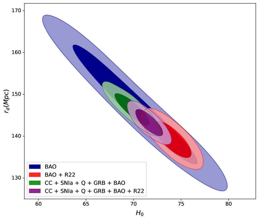
(a) $\Lambda$CDM Model

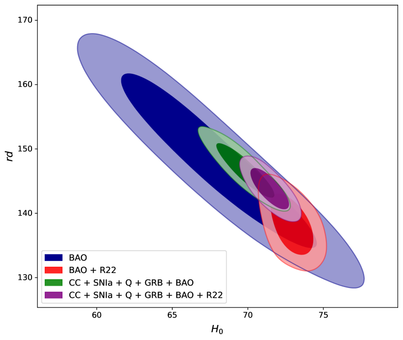
(b) VsMCG Model

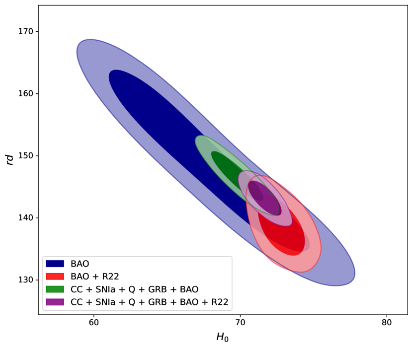
(c) VMCG Model

Figure 5: The figure shows the posterior distribution of diverse observational data measurements within the $r_{d}-H_{0}$ contour plane using the $\Lambda$CDM, VsMCG and VMCG models. The shaded regions correspond to the 1$\sigma$ and 2$\sigma$ confidence plane.

IV Gravitational Lensing

The differential probability that a distribution of galaxies per unit redshift will be multiply imaged by a source with redshift $z_{s}$ is [33]:

$$\frac{d\tau}{dz_{l}}=n(1+z_{l})^{3}S\frac{cdt}{dz_{l}}$$ (16)

where $n$ denotes the co-moving number density of lenses, $S$ is the lens cross-section and $cdt/dz_{l}$ the proper distance interval. Further, following numerous work [29, 56] done previously, we assume an singular isothermal sphere (SIS) profile for our lensing model. Thus, the expression for lensing cross-section in an SIS profile is given by:

$$S=16\pi^{3}\left(\frac{\sigma}{c}\right)^{4}\left(\frac{D_{l}D_{ls}}{D_{s}}\right)^{2}$$ (17)

where $\sigma$ is the velocity dispersion, $D_{s}$, $D_{l}$ and $D_{ls}$ represents the angular diameter distances between observer-source, observer-lens and lens-source respectively, given by:

$$D_{z_{1}z_{2}}=\frac{1}{\sqrt{H_{0}}(1+z_{2})}\int_{z_{1}}^{z_{2}}\frac{1}{\sqrt{H(z)}}dz\hskip 28.45274pt(k=0)$$ (18)

and finally the proper distance interval reads:

$$\frac{cdt}{dz_{l}}=\frac{c}{(1+z_{l})H(z_{l})}$$ (19)

Now, in order to calculate $n$ present in Eq. (16), we use the Schechter function given by:

$$\frac{dn}{dL}=\frac{n^{*}_{i}}{L^{*}_{i}}{\left(\frac{L}{L_{i}^{*}}\right)}^{\gamma_{i}}e^{(-L/L_{i}^{*})}$$ (20)

where $i$ depends on the type of galaxy morphology (i.e. $S,S_{0}$ or $E$, $n_{i}^{*}$ denotes the characteristic number density, and $l_{i}^{*}$ the characteristic luminosity. Additionally, with the help of the power-law relation $L/L_{i}^{*}=(\sigma/\sigma_{i}^{*})^{g_{i}}$, equation (20) further reduces to

$$\frac{dn}{d\sigma}=\frac{n^{*}_{i}}{\sigma^{*}_{i}}{\left(\frac{\sigma}{\sigma_{i}^{*}}\right)}^{g_{i}\gamma_{i}+g_{i}-1}e^{(-\sigma/\sigma_{i}^{*})^{g_{i}}}g_{i}$$ (21)

Thus, the differential optical depth can now be obtained by integrating eqn. (16) from $0$ to $z_{s}$ as follows:

$$\tau(z_{s})=\left(\sum_{i=S,S_{0},E}F_{i}\right)\int_{0}^{\chi_{s}}\left(\frac{\chi_{s}-\chi_{l}}{\chi_{s}}\right)^{2}\chi_{l}^{2}d\chi_{l}$$ (22)

where

$$\chi_{i}=\sqrt{H_{0}}\int_{0}^{z_{i}}\frac{dz}{\sqrt{H(z)}}$$ (23)

is the co-moving distances, $F_{i}$ represents the ability of the $i$th class of galaxy morphology to produce multiple images, relying exclusively on the intrinsic and statistical properties of the galaxies. Using equation (21), we may calculate $F_{i}$ in the form:

$$\begin{split}F_{i}&=16\pi^{3}\sigma^{4}H_{0}^{-3}\int_{0}^{\infty}\frac{n^{*}_{i}}{\sigma^{*}_{i}}{\left(\frac{\sigma}{\sigma_{i}^{*}}\right)}^{g_{i}\alpha_{i}+g_{i}-1}e^{(-\sigma/\sigma_{i}^{*})^{g_{i}}}g_{i}d\sigma\\ &=16\pi^{3}\sigma^{4}H_{0}^{-3}n_{i}^{*}\Gamma(\alpha_{i}+1)\end{split}$$ (24)

Considering the uncertainties extensively addressed in the literature [57, 58, 59, 60], we will treat $F$ to be a normalized factor, denoted as $F\equiv\sum_{i=S,S_{0},E}F_{i}$. Therefore, from equations (22) and (24), we deduce a straightforward analytical expression for the optical depth of a point source at redshift $z_{s}$ in an FRW Universe with dark matter and dark energy components [33]:

$$\tau(z_{s})=\frac{F}{30}\chi_{s}^{3}$$ (25)

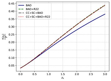
Figure 6: Variation in optical depth behaviour of VsMCG model w.r.t $z_{s}$ for parameters constrained through different data sets given in Table 2.

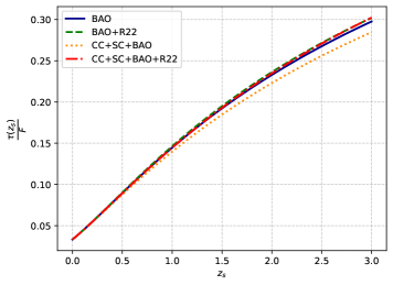
Figure 7: Variation in optical depth behaviour of VMCG model w.r.t $z_{s}$ for parameters constrained through different data sets given in Table 2.

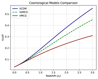
Figure 8: Variation in optical depth behaviour of $\Lambda$CDM ($H_{0}=71.67,\Omega_{m0}=0.26$), VsMCG ($H_{0}=72.86,\Omega_{m0}=0.28,A_{s}=0.44,\alpha=0.66,A=3.09,\zeta=2.05,\rho_{1}=1.35351\times 10^{6}$) and VMCG ($H_{0}=74.02,\Omega_{m0}=0.18,n=0.97,\beta=1.02,C=0.03,C_{s}=0.48,\rho_{1}=1.35085\times 10^{6}$) model w.r.t source redshift $z_{s}$.

V Results

For the standard $\Lambda$CDM model, the posterior distribution of the key cosmological parameters is shown at the $68\%$ and $95\%$ confidence levels in Fig. 2. Detailed results from MCMC simulations are outlined in Table 2. When the R22 prior is incorporated into the joint dataset, the optimal fitting value for $H_{0}$ is $71.50\pm 0.882$, diverging [15] from but aligning closely with measurements from the SNIe sample in [53]. In the absence of R22 priors with the Joint dataset, the estimated $H_{0}=69.837\pm 1.204$ corresponds more closely to the value in [15]. Figs 3 and 4 portray the $68\%$ and $95\%$ confidence levels for crucial cosmological parameters in VsMCG and VMCG models. Across these models, when the R22 prior is included in the Joint dataset, the optimal fitting value for $H_{0}$ diverges from [15] but aligns more closely with the SNIe sample in [53]. Conversely, without R22 priors and using the Joint dataset, the estimated $H_{0}=69.837\pm 1.204$ aligns more closely with [15]. The determined values for the matter density, denoted as $\Omega_{m0}$, and the dark energy density, denoted as $\Omega_{d0}$, in the $\Lambda$CDM and VMCG Models, appear to be lower compared to the values documented in [15] ($\Omega_{m0}=0.315\pm 0.007$, $\Omega_{d0}=0.685\pm 0.007$). However, in the case of the VsMCG Model, it is higher than the value documented in [15]. However, this observation has been documented in alternative studies [61, 62]. In the context of the Baryon Acoustic Oscillations (BAO) scale, it is defined by the cosmic sound horizon imprinted in the cosmic microwave background during the drag epoch, denoted as $z_{d}$. This epoch marks the separation of baryons and photons. The BAO scale, represented by $r_{d}$, is determined by the integral of the ratio of the speed of sound ($c_{s}$) to the Hubble parameter ($H_{0}$) over the redshift range from $z_{d}$ to infinity. The speed of sound, $c_{s}$, is given by $\sqrt{\frac{\delta p_{\gamma}}{\delta\rho_{B}+\delta\rho_{\gamma}}}$, where $\delta p_{\gamma}$ is the pressure perturbation in photons, and $\delta\rho_{B}$ and $\delta\rho_{\gamma}$ are perturbations in the baryon and photon energy densities, respectively. This expression is further simplified to $\frac{1}{\sqrt{3(1+R)}}$, with $R$ defined as the ratio of baryon density perturbation to photon density perturbation ($R\equiv\frac{\delta\rho_{B}}{\delta\rho_{\gamma}}=\frac{3\rho_{B}}{4\rho_{\gamma}}$). Observational data from [15] provides the redshift at the drag epoch as $z_{d}=1059.94\pm 0.30$. In the case of a $\Lambda$CDM model, measurements from [15] estimate the BAO scale $r_{d}$ to be $147.09\pm 0.26$ megaparsecs (Mpc). In our exploration of the $\Lambda$CDM model, Fig 5(a) illustrates the posterior distribution of the contour plane for $r_{d}-H_{0}$. The BAO datasets provide an estimated $r_{d}$ of $145.807\pm 9.06$ Mpc, aligning with the reported findings in [63]. However, when we exclusively incorporate R22 prior into the BAO dataset, the determined sound horizon at the drag epoch is $138.345\pm 2.45$ Mpc. Examining the Joint dataset reveals an estimated BAO scale ($r_{d}$) of $145.811\pm 2.34$ Mpc, closely aligning with the outcomes reported in [15]. Additionally, incorporating the R22 prior into the comprehensive dataset results in $r_{d}$ of $142.591\pm 1.49$ Mpc, indicating proximity to the findings in [64]. Now, shifting to the VsMCG Model, Fig 5(b) presents the posterior distribution for the $r_{d}-H_{0}$ contour plane. For the BAO datasets, the resulting $r_{d}$ is $149.571\pm 8.752$ Mpc, consistent with the Planck results as reported in [63]. However, incorporating R22 prior exclusively into the BAO dataset leads to a sound horizon at the drag epoch of $140.757\pm 8.454$ Mpc. In the case of the Joint dataset, the determined $r_{d}$ is $147.559\pm 2.72$ Mpc, aligning closely with the Planck results. Furthermore, integrating the R22 prior into the full dataset results in $r_{d}=141.158\pm 2.299$ Mpc, showing proximity to the findings presented in [64]. In the context of the VMCG Model, Fig 5(c) illustrates the posterior distribution of the $r_{d}-H_{0}$ contour plane. When considering BAO datasets, the estimated BAO scale ($r_{d}$) is $148.683\pm 8.949$ Mpc, a result consistent with the findings reported in [63]. However, introducing the R22 prior into the BAO dataset alone yields a sound horizon at the drag epoch of $139.365\pm 9.762$ Mpc. In the case of the Joint dataset, the calculated BAO scale ($r_{d}$) is $147.906\pm 2.386$ Mpc, which closely matches the results obtained from the Planck mission. Additionally, when we include the R22 prior in the complete dataset, the resulting $r_{d}$ is $141.623\pm 2.638$ Mpc, indicating a close agreement with the findings reported in [64]. The results from $\Lambda$CDM, VsMCG and VMCG models exhibit tension with the $r_{d}$ value estimated by Planck. However, these results still demonstrate agreement with the findings presented in [64] reports that by employing Binning and Gaussian methods to combine measurements of 2D BAO and SNIa data, the values of the absolute $\mathrm{BAO}$ scale range from 141.45 Mpc to $r_{d}\leq 159.44\mathrm{Mpc}$ (Binning) and 143.35 Mpc to $r_{d}\leq 161.59\mathrm{Mpc}$ (Gaussian). These findings highlight a clear discrepancy between early and late-time observational measurements, analogous to the $H_{0}$ tension. It is noteworthy that our results are contingent on the range of priors for $r_{d}$ and $H_{0}$, influencing the estimated values in the $r_{d}-H_{0}$ contour plane. An interesting observation is that when we exclude the R22 prior, the results for $H_{0}$ and $r_{d}$ tend to align with the Planck and SDSS results, mitigating the tension observed in the absence of this particular prior.

Now, in the study of the gravitational lensing optical depth, we use the analytical expression given by eqn. (25). After constraining the model parameters of the DE models as discussed above and finding their best-fit values, we plot the graphs of $\tau(z_{s})/F$ against redshift $z_{s}$ for both models. Figs. 6 and 7, respectively, show changes in the optical depth behaviour of the two DE models here w.r.t $z_{s}$. We notice that the probability of finding gravitational lenses (i.e. optical depth) increases for both the models with increasing $z_{s}$ value. Further, from fig. 6, we observe that the graphs of $\tau(z_{s})$ for parameter sets constrained through different data sets show similar behaviour except for the parameters constraint through $BAO$ only. However, for $z_{s}<1$, they all coincide with each other. From these, we can conclude that the parameter values constraint through different data sets have very little to no effect in detecting the distribution of gravitational lenses in our Universe. Again, if we analyse fig. 7, we observe that parameters constrained through the combination of $CC+SC+BAO+R22$ give a lower probability of finding gravitational lenses as compared to the other three combinations. However, for the other three combinations of data sets, viz. $BAO,BAO+R22,CC+SC+BAO$, we can observe small deviations in $\tau(z_{s})$ for higher redshift values but for $z_{s}<1$, the graph shows same lensing probability. This implies that in this DE model, parameter values constrained through $CC+SC+BAO+R22$ data sets give a slightly better approximation of the distribution of gravitational lenses than the rest. Finally, we conclude our study by plotting the optical depth of the two DE models considered here along with $\Lambda$CDM against source redshift $z_{s}$. We observe from Fig. 8 that although at the present epoch, the gravitational lensing probability for the three models coincides with each other, however moving back in time (or higher redshift values), all the models highly diverge from each other with $\Lambda$CDM gives the highest lensing probability and VMCG the lowest.

VI Discussions and Conclusions

Assuming our Universe to be filled with dark matter and dark energy combinations in a flat FRW Universe, we reviewed two models of modified Chaplygin gas as the fluid source. For the dark energy candidates, we considered viscous modified Chaplygin gas (VsMCG) and variable modified Chaplygin gas (VMCG) in the framework of loop quantum cosmology. We determined the respective Hubble parameter and, consequently, constraint the associated model parameters with the help of the latest observational data. Our investigation involved the selection of 24 Baryon Acoustic Oscillation (BAO) points were deliberately chosen to minimize correlations from an extensive dataset comprising 333 BAO data points. The objective was to mitigate inherent errors in the posterior distribution, which could potentially stem from correlations between measurements. Employing a method that mimics the introduction of random correlations into the covariance matrix, we conducted a systematic procedure. Our subsequent verification process attested that these introduced correlations do not lead to substantial alterations in the resulting cosmological parameters. Furthermore, we incorporated a variety of datasets into our analysis. This involved the inclusion of 30 uncorrelated data points from Cosmic Chronometers, a carefully selected set of 40 points obtained from Type Ia supernovae, 24 points extracted from the Hubble diagram for quasars, and a considerable dataset consisting of 162 points derived from Gamma Ray Bursts. Additionally, we integrated the most recent measurement of the Hubble constant conducted by researcher R22. Our recent investigation, conducted through a comprehensive array of observational assessments, brings attention to the persistent existence of the Hubble tension, although it is somewhat mitigated to a $2\sigma$ level for $H_{0}$. By introducing the sound horizon ($r_{d}$) as a free parameter, we have derived specific values for $H_{0}$ and $r_{d}$ in various cosmological models, including the Standard $\Lambda$CDM, VsMCG, and VMCG models. In the $\Lambda$CDM model, our analysis reveals $H_{0}=69.828145\pm 1.009964\ \mathrm{km/s/Mpc}$ and $r_{d}=146.826212\pm 2.201612\ \mathrm{Mpc}$. For the VsMCG model, we obtain $H_{0}=67.447204\pm 8.878032\ \mathrm{km/s/Mpc}$ and $r_{d}=147.559044\pm 2.723020\ \mathrm{Mpc}$. Similarly, in the case of VMCG, the results indicate $H_{0}=69.204717\pm 8.056031\ \mathrm{km/s/Mpc}$ and $r_{d}=147.906003\pm 2.386071\ \mathrm{Mpc}$. Crucially, our assessments highlight that the values of $H_{0}$ and $r_{d}$ based on low-redshift measurements align with early Planck estimates [15]. We also studied the gravitational lensing optical depth of our two dark energy models with the help of the constrained model parameter values. The graph showing changes in optical depth is plotted against their source redshift (fig. 6 & 7). For both models, the probability of finding gravitational lenses increases with higher redshift values. However, for low redshift ($z_{s}<1$), the lensing probability in both the DE models coincides irrespective of the different sets of constrained parameter values obtained by considering different combinations of data sets. Lastly, we also carried out a joint analysis of the two DE models considered here with that of $\Lambda$CDM model (fig. 8). We found that the three models are indistinguishable for low redshift value ($z_{s}<1)$; however, they highly diverge from each other in the early Universe. Finally, we conclude our study with a statistical evaluation of our cosmological models and utilize both the Akaike Information Criterion (AIC) and the Bayesian Information Criterion (BIC). The AIC is expressed as [65, 66]: $\mathrm{AIC}=-2\ln(\mathcal{L}_{\text{max}})+2k+\frac{2k(2k+1)}{N_{\text{tot}}-k-1}$ Here, $\mathcal{L}_{\max}$ signifies the maximum likelihood of the data, incorporating the entire dataset without the R22 prior. The parameters encompass $N_{\text{tot}}$, the total number of data points (in our instance, $N_{\text{tot}}=296$), and $k$, the number of parameters. For large $N_{\text{tot}}$, this expression simplifies to:$\mathrm{AIC}\simeq-2\ln(\mathcal{L}_{\max})+2k$ which is the conventional form of the AIC criterion [65]. In contrast, the Bayesian Information Criterion is formulated as [66]: $\mathrm{BIC}=-2\ln(\mathcal{L}_{\max})+k\ln N_{\text{tot}}$. By applying these criteria, we compute the AIC and BIC for the standard $\Lambda$CDM, VsMCG, and VMCG models. The obtained values for $\Lambda$CDM, VsMCG, and VMCG models are, respectively AIC = $[277.38,281.16,281.12]$ and BIC = $[277.59,283.12,282.34]$. Despite the $\Lambda$CDM model displaying the best fit due to the lowest AIC, our collective AIC and BIC results lend support to all the tested models. This suggests that none of the models can be dismissed based on the existing data. In the evaluation of the VsMCG and VMCG models relative to $\Lambda$CDM, we acknowledge that $\Lambda$CDM is embedded within both proposed extensions, differing by 5 degrees of freedom. This distinction allows for the application of standard statistical tests. The yardstick for comparison is the reduced chi-square statistic, defined as $\chi_{\text{red}}^{2}=\chi^{2}/\text{Dof}$, where Dof represents the degrees of freedom of the model, and $\chi^{2}$ denotes the weighted sum of squared deviations with an equal number of runs for the three models, the statistic approximates 1, expressed as: $\left(\frac{\chi^{2}}{Dof_{\Lambda CDM}},\frac{\chi^{2}}{Dof_{VsMCG}},\frac{\chi^{2}}{Dof_{VMCG}}\right)\approx\{0.961646,0.971234,0.954310\}$. This comparative analysis offers valuable insights into the goodness of fit for each model, with values near 1 signifying a satisfactory alignment with the observed data. The findings suggest that both the VsMCG and VMCG models provide viable alternatives to the standard $\Lambda$CDM model, with comparable goodness of fit and support from statistical criteria.

References

- [1] A. G. Riess, A. V. Filippenko, and et al., “Observational evidence from supernovae for an accelerating universe and a cosmological constant,” Astron. J., vol. 116, no. 3, p. 1009, 1998.
- [2] D. N. Spergel, L. Verde, and et al., “First-year Wilkinson Microwave Anisotropy Probe (WMAP)* observations: determination of cosmological parameters,” Astrophys. J. Suppl. Ser., vol. 148, no. 1, p. 175, 2003.
- [3] A. R. Liddle and D. H. Lyth, Cosmological inflation and large-scale structure. Cambridge university press, 2000.
- [4] E. Komatsu, J. Dunkley, and et al., “FIVE-YEAR WILKINSON MICROWAVE ANISOTROPY PROBE OBSERVATIONS: COSMOLOGICAL INTERPRETATION,” Astrophys. J. Suppl. Ser., vol. 180, pp. 330–376, feb 2009.
- [5] A. Kamenshchik, U. Moschella, and V. Pasquier, “An alternative to quintessence,” Physics Letters B, vol. 511, no. 2-4, pp. 265–268, 2001.
- [6] U. Debnath, A. Banerjee, and S. Chakraborty, “Role of modified chaplygin gas in accelerated universe,” Classical and Quantum Gravity, vol. 21, no. 23, p. 5609, 2004.
- [7] P. Peebles and B. Ratra, “Cosmology with a time-variable cosmological’constant’,” Astrophysical Journal, Part 2-Letters to the Editor (ISSN 0004-637X), vol. 325, Feb. 15, 1988, p. L17-L20. NSF-supported research., vol. 325, pp. L17–L20, 1988.
- [8] R. R. Caldwell, R. Dave, and P. J. Steinhardt, “Cosmological imprint of an energy component with general equation of state,” Physical Review Letters, vol. 80, no. 8, p. 1582, 1998.
- [9] U. Alam, V. Sahni, T. Deep Saini, and A. A. Starobinsky, “Is there supernova evidence for dark energy metamorphosis?,” Monthly Notices of the Royal Astronomical Society, vol. 354, no. 1, pp. 275–291, 2004.
- [10] S. D. Hsu, “Entropy bounds and dark energy,” Phys. Lett. Sect. B Nucl. Elem. Part. High-Energy Phys., vol. 594, no. 1-2, pp. 13–16, 2004.
- [11] M. Li, “A model of holographic dark energy,” Phys. Lett. Sect. B Nucl. Elem. Part. High-Energy Phys., vol. 603, no. 1-2, pp. 1–5, 2004.
- [12] E. J. COPELAND, M. SAMI, and S. TSUJIKAWA, “DYNAMICS OF DARK ENERGY,” Int. J. Mod. Phys. D, vol. 15, pp. 1753–1935, nov 2006.
- [13] V. Springel, C. S. Frenk, and S. D. White, “The large-scale structure of the universe,” nature, vol. 440, no. 7088, pp. 1137–1144, 2006.
- [14] A. Jenkins, C. Frenk, F. Pearce, P. Thomas, J. Colberg, S. D. White, H. Couchman, J. Peacock, G. Efstathiou, and A. Nelson, “Evolution of structure in cold dark matter universes,” The Astrophysical Journal, vol. 499, no. 1, p. 20, 1998.
- [15] P. Collaboration, N. Aghanim, Y. Akrami, M. Ashdown, J. Aumont, C. Baccigalupi, M. Ballardini, A. Banday, R. Barreiro, N. Bartolo, et al., “Planck 2018 results. vi. cosmological parameters,” 2020.
- [16] A. G. Riess, A. V. Filippenko, P. Challis, A. Clocchiatti, A. Diercks, P. M. Garnavich, R. L. Gilliland, C. J. Hogan, S. Jha, R. P. Kirshner, et al., “Observational evidence from supernovae for an accelerating universe and a cosmological constant,” The astronomical journal, vol. 116, no. 3, p. 1009, 1998.
- [17] D. J. Eisenstein and W. Hu, “Baryonic features in the matter transfer function,” The Astrophysical Journal, vol. 496, no. 2, p. 605, 1998.
- [18] P. J. Peebles and J. Yu, “Primeval adiabatic perturbation in an expanding universe,” Astrophysical Journal, vol. 162, p. 815, vol. 162, p. 815, 1970.
- [19] D. J. Eisenstein, I. Zehavi, D. W. Hogg, R. Scoccimarro, M. R. Blanton, R. C. Nichol, R. Scranton, H.-J. Seo, M. Tegmark, Z. Zheng, et al., “Detection of the baryon acoustic peak in the large-scale correlation function of sdss luminous red galaxies,” The Astrophysical Journal, vol. 633, no. 2, p. 560, 2005.
- [20] S. Alam, F. D. Albareti, C. A. Prieto, F. Anders, S. F. Anderson, T. Anderton, B. H. Andrews, E. Armengaud, É. Aubourg, S. Bailey, et al., “The eleventh and twelfth data releases of the sloan digital sky survey: final data from sdss-iii,” The Astrophysical Journal Supplement Series, vol. 219, no. 1, p. 12, 2015.
- [21] S. NOJIRI and S. D. ODINTSOV, “INTRODUCTION TO MODIFIED GRAVITY AND GRAVITATIONAL ALTERNATIVE FOR DARK ENERGY,” Int. J. Geom. Methods Mod. Phys., vol. 04, pp. 115–145, feb 2007.
- [22] S. Capozziello and M. De Laurentis, “Extended Theories of Gravity,” Phys. Rep., vol. 509, pp. 167–321, dec 2011.
- [23] A. Ashtekar and J. Lewandowski, “Background independent quantum gravity: a status report,” Classical and Quantum Gravity, vol. 21, no. 15, p. R53, 2004.
- [24] M. Bojowald, “Loop quantum cosmology,” Living Reviews in Relativity, vol. 11, pp. 1–131, 2008.
- [25] M. Jamil and U. Debnath, “Interacting modified chaplygin gas in loop quantum cosmology,” Astrophysics and Space Science, vol. 333, pp. 3–8, 2011.
- [26] X. Fu, H. Yu, and P. Wu, “Dynamics of interacting phantom scalar field dark energy in loop quantum cosmology,” Physical Review D, vol. 78, no. 6, p. 063001, 2008.
- [27] S. Refsdal and H. Bondi, “The gravitational lens effect,” Monthly Notices of the Royal Astronomical Society, vol. 128, no. 4, pp. 295–306, 1964.
- [28] E. L. Turner, J. P. Ostriker, and J. R. Gott III, “The statistics of gravitational lenses-the distributions of image angular separations and lens redshifts,” The Astrophysical Journal, vol. 284, pp. 1–22, 1984.
- [29] J. R. Gott III, M.-G. Park, and H. M. Lee, “Setting limits on q0 from gravitational lensing,” Astrophysical Journal, Part 1 (ISSN 0004-637X), vol. 338, March 1, 1989, p. 1-12., vol. 338, pp. 1–12, 1989.
- [30] Z.-H. Zhu, “Gravitational lensing statistical properties in general frw cosmologies with dark energy component (s): analytic results,” International Journal of Modern Physics D, vol. 9, no. 05, pp. 591–600, 2000.
- [31] Z.-H. Zhu, “Gravitational lensing statistics as a probe of dark energy,” Modern Physics Letters A, vol. 15, no. 16, pp. 1023–1029, 2000.
- [32] R. Freitas, S. Gonçalves, and A. Oliveira, “Gravitational lenses in the dark universe,” Astrophysics and Space Science, vol. 349, pp. 443–455, 2014.
- [33] R. Kundu, U. Debnath, and A. Pradhan, “Gravitational lensing: dark energy models in non-flat frw universe,” The European Physical Journal C, vol. 83, no. 6, p. 553, 2023.
- [34] D. Aberkane, N. Mebarki, and S. Benchikh, “Viscous modified chaplygin gas in classical and loop quantum cosmology,” Chinese Physics Letters, vol. 34, no. 6, p. 069801, 2017.
- [35] U. Debnath, “Variable modified chaplygin gas and accelerating universe,” Astrophysics and Space Science, vol. 312, no. 3-4, pp. 295–299, 2007.
- [36] A. J. Ross, L. Samushia, C. Howlett, W. J. Percival, A. Burden, and M. Manera, “The clustering of the sdss dr7 main galaxy sample–i. a 4 per cent distance measure at z= 0.15,” Monthly Notices of the Royal Astronomical Society, vol. 449, no. 1, pp. 835–847, 2015.
- [37] S. Alam, M. Ata, S. Bailey, F. Beutler, D. Bizyaev, J. A. Blazek, A. S. Bolton, J. R. Brownstein, A. Burden, C.-H. Chuang, et al., “The clustering of galaxies in the completed sdss-iii baryon oscillation spectroscopic survey: cosmological analysis of the dr12 galaxy sample,” Monthly Notices of the Royal Astronomical Society, vol. 470, no. 3, pp. 2617–2652, 2017.
- [38] H. Gil-Marín, J. E. Bautista, R. Paviot, M. Vargas-Magaña, S. de La Torre, S. Fromenteau, S. Alam, S. Ávila, E. Burtin, C.-H. Chuang, et al., “The completed sdss-iv extended baryon oscillation spectroscopic survey: measurement of the bao and growth rate of structure of the luminous red galaxy sample from the anisotropic power spectrum between redshifts 0.6 and 1.0,” Monthly Notices of the Royal Astronomical Society, vol. 498, no. 2, pp. 2492–2531, 2020.
- [39] A. Raichoor, A. De Mattia, A. J. Ross, C. Zhao, S. Alam, S. Avila, J. Bautista, J. Brinkmann, J. R. Brownstein, E. Burtin, et al., “The completed sdss-iv extended baryon oscillation spectroscopic survey: large-scale structure catalogues and measurement of the isotropic bao between redshift 0.6 and 1.1 for the emission line galaxy sample,” Monthly Notices of the Royal Astronomical Society, vol. 500, no. 3, pp. 3254–3274, 2021.
- [40] J. Hou, A. G. Sánchez, A. J. Ross, A. Smith, R. Neveux, J. Bautista, E. Burtin, C. Zhao, R. Scoccimarro, K. S. Dawson, et al., “The completed sdss-iv extended baryon oscillation spectroscopic survey: Bao and rsd measurements from anisotropic clustering analysis of the quasar sample in configuration space between redshift 0.8 and 2.2,” Monthly Notices of the Royal Astronomical Society, vol. 500, no. 1, pp. 1201–1221, 2021.
- [41] H. D. M. Des Bourboux, J. Rich, A. Font-Ribera, V. de Sainte Agathe, J. Farr, T. Etourneau, J.-M. Le Goff, A. Cuceu, C. Balland, J. E. Bautista, et al., “The completed sdss-iv extended baryon oscillation spectroscopic survey: baryon acoustic oscillations with ly forests,” The Astrophysical Journal, vol. 901, no. 2, p. 153, 2020.
- [42] T. Abbott, M. Aguena, S. Allam, A. Amon, F. Andrade-Oliveira, J. Asorey, S. Avila, G. Bernstein, E. Bertin, A. Brandao-Souza, et al., “Dark energy survey year 3 results: A 2.7% measurement of baryon acoustic oscillation distance scale at redshift 0.835,” Physical Review D, vol. 105, no. 4, p. 043512, 2022.
- [43] S. Sridhar, Y.-S. Song, A. J. Ross, R. Zhou, J. A. Newman, C.-H. Chuang, R. Blum, E. Gaztanaga, M. Landriau, and F. Prada, “Clustering of lrgs in the decals dr8 footprint: Distance constraints from baryon acoustic oscillations using photometric redshifts,” The Astrophysical Journal, vol. 904, no. 1, p. 69, 2020.
- [44] F. Beutler, C. Blake, M. Colless, D. H. Jones, L. Staveley-Smith, L. Campbell, Q. Parker, W. Saunders, and F. Watson, “The 6df galaxy survey: baryon acoustic oscillations and the local hubble constant,” Monthly Notices of the Royal Astronomical Society, vol. 416, no. 4, pp. 3017–3032, 2011.
- [45] L. Kazantzidis and L. Perivolaropoulos, “Evolution of the f 8 tension with the planck 15/cdm determination and implications for modified gravity theories,” Physical Review D, vol. 97, no. 10, p. 103503, 2018.
- [46] M. Moresco, “Raising the bar: new constraints on the hubble parameter with cosmic chronometers at z 2,” Monthly Notices of the Royal Astronomical Society: Letters, vol. 450, no. 1, pp. L16–L20, 2015.
- [47] M. Moresco, L. Pozzetti, A. Cimatti, R. Jimenez, C. Maraston, L. Verde, D. Thomas, A. Citro, R. Tojeiro, and D. Wilkinson, “A 6% measurement of the hubble parameter at z 0.45: direct evidence of the epoch of cosmic re-acceleration,” Journal of Cosmology and Astroparticle Physics, vol. 2016, no. 05, pp. 014–014, 2016.
- [48] M. Moresco, L. Verde, L. Pozzetti, R. Jimenez, and A. Cimatti, “New constraints on cosmological parameters and neutrino properties using the expansion rate of the universe to z 1.75,” Journal of Cosmology and Astroparticle Physics, vol. 2012, no. 07, p. 053, 2012.
- [49] M. Moresco, A. Cimatti, R. Jimenez, L. Pozzetti, G. Zamorani, M. Bolzonella, J. Dunlop, F. Lamareille, M. Mignoli, H. Pearce, et al., “Improved constraints on the expansion rate of the universe up to z 1.1 from the spectroscopic evolution of cosmic chronometers,” Journal of Cosmology and Astroparticle Physics, vol. 2012, no. 08, pp. 006–006, 2012.
- [50] D. M. Scolnic, D. Jones, A. Rest, Y. Pan, R. Chornock, R. Foley, M. Huber, R. Kessler, G. Narayan, A. Riess, et al., “The complete light-curve sample of spectroscopically confirmed sne ia from pan-starrs1 and cosmological constraints from the combined pantheon sample,” The Astrophysical Journal, vol. 859, no. 2, p. 101, 2018.
- [51] C. Roberts, K. Horne, A. O. Hodson, and A. D. Leggat, “Tests of cdm and conformal gravity using grb and quasars as standard candles out to ,” arXiv preprint arXiv:1711.10369, 2017.
- [52] M. Demianski, E. Piedipalumbo, D. Sawant, and L. Amati, “Cosmology with gamma-ray bursts-ii. cosmography challenges and cosmological scenarios for the accelerated universe,” Astronomy & Astrophysics, vol. 598, p. A113, 2017.
- [53] A. G. Riess, W. Yuan, L. M. Macri, D. Scolnic, D. Brout, S. Casertano, D. O. Jones, Y. Murakami, G. S. Anand, L. Breuval, et al., “A comprehensive measurement of the local value of the hubble constant with 1 km s- 1 mpc- 1 uncertainty from the hubble space telescope and the sh0es team,” The Astrophysical journal letters, vol. 934, no. 1, p. L7, 2022.
- [54] W. Handley, M. Hobson, and A. Lasenby, “Polychord: nested sampling for cosmology,” Monthly Notices of the Royal Astronomical Society: Letters, vol. 450, no. 1, pp. L61–L65, 2015.
- [55] A. Lewis, “Getdist: a python package for analysing monte carlo samples,” arXiv preprint arXiv:1910.13970, 2019.
- [56] J. R. Gott III and J. E. Gunn, “The double quasar 1548+ 115a, b as a gravitational lens,” Astrophysical Journal, vol. 190, p. L105, vol. 190, p. L105, 1974.
- [57] E. L. Turner, “Gravitational lensing limits on the cosmological constant in a flat universe,” Astrophys. J., vol. 365, pp. L43—-L46, 1990.
- [58] M. Fukugita, T. Futamase, and M. Kasai, “A possible test for the cosmological constant with gravitational lenses,” Mon. Not. R. Astron. Soc., vol. 246, p. 24P, 1990.
- [59] L. M. Krauss and M. White, “Gravitational lensing, finite galaxy cores, and the cosmological constant,” Astrophys. J., vol. 394, pp. 385–395, 1992.
- [60] C. S. Kochanek, “Analytic results for the gravitational lens statistics of singular isothermal spheres in general cosmologies,” Mon. Not. R. Astron. Soc., vol. 261, no. 2, pp. 453–463, 1993.
- [61] R. C. Nunes, S. K. Yadav, J. Jesus, and A. Bernui, “Cosmological parameter analyses using transversal bao data,” Monthly Notices of the Royal Astronomical Society, vol. 497, no. 2, pp. 2133–2141, 2020.
- [62] R. C. Nunes and A. Bernui, “Bao signatures in the 2-point angular correlations and the hubble tension,” The European Physical Journal C, vol. 80, pp. 1–8, 2020.
- [63] L. Verde, J. L. Bernal, A. F. Heavens, and R. Jimenez, “The length of the low-redshift standard ruler,” Monthly Notices of the Royal Astronomical Society, vol. 467, no. 1, pp. 731–736, 2017.
- [64] T. Lemos, Ruchika, J. C. Carvalho, and J. Alcaniz, “Low-redshift estimates of the absolute scale of baryon acoustic oscillations,” The European Physical Journal C, vol. 83, no. 6, p. 495, 2023.
- [65] H. Akaike, “A new look at the statistical model identification,” IEEE transactions on automatic control, vol. 19, no. 6, pp. 716–723, 1974.
- [66] G. Schwarz, “Estimating the dimension of a model,” The annals of statistics, pp. 461–464, 1978.