Naked singularities and black hole Killing horizons

Abstract

In this chapter, we study special photon orbits defined by means of Killing vectors and present a framework based on the properties of such null orbits. For concreteness, we restrict ourselves to the case of axially symmetric spacetimes describing either black holes with Killing horizons or naked singularities. The null-orbits framework is then applied to analyze properties of naked singularities and concepts of black hole thermodynamics.

0.1 Introduction

The creation of a naked singularity (NS) through accretion onto a (extreme) black hole (BH) is forbidden. In particular, the horizon area cannot decrease in any process with suitable conditions on the energy and no repulsive gravity. More precisely, the total horizon area of (classical) BHs cannot decrease over time (Hawking’s area theorem -Hawking71 ; Hawking74 ; Hawking75 ). Observational data of GW150914 have been recently considered as an observational confirmation of Hawking’s black-hole area theorem– Isi:2020tac . However, assuming the existence of NSs, the reverse process, consisting in the conversion, at some point of the singularity formation or evolution, into a BH is still debated in different contexts. A classical method for extracting energy from a spinning BH and from a hypothetical NS is, for example, the Penrose process, which is based on the frame-dragging effects of the ergoregion of a spinning BH –Penrose69 . In this region, a small body may have negative energy, as measured by an observer at infinity and, if fragmented into two parts, and the part with negative-energy will be swallowed by the BH, it will decrease its (total) mass, while the other part, with positive energy, can be ejected. In this process, the Kerr BH rotational energy decreases and consequently, the Kerr BH area (determined by its outer horizon) increases.

In this chapter, we focus on BH spacetimes with Killing horizons and on naked singularity solutions of the corresponding field equations. It is possible to study the singularities using light surfaces related to the background Killing fields, and in particular to the generators of Killing horizons. Special null orbits associated to the Killing vectors of the geometry can generate a useful framework for the study of the more diverse geometries, such as wormholes, accelerating black holes, or binary black hole systems, pointing out the existence of common properties of the light surfaces in different spacetimes.

Here, we will use the properties of the Killing vectors, generators of the BH Killing horizons, limiting ourselves to the cases of the Kerr and Kerr–Newman spacetimes.

The Kerr-Newman (KN) solution is an electrically charged, electro–vacuum, asymptotically flat, axially symmetric (and stationary) solution of the Einstein–Maxwell equations, used to describe the spacetime around an electrically charged gravitational source, spinning along it symmetry axis. The Kerr solution can be read as a limit of the KN metric when the electric charge is null. According to the ”no–hair” theorems, the Einstein–Maxwell BH solutions are characterized only by mass, electric charge, and angular momentum; therefore the Kerr–Newman spacetime is the most general asymptotically flat stationary BH solution of the Einstein–Maxwell equations. On the other hand, there are other stationary axisymmetric solutions of the Einstein–Maxwell equations with additional parameters, such as acceleration, magnetic charge, NUT charge, and cosmological constant, having therefore up to seven parameters. Furthermore, the theorem has been proved to be violated, for example, by the self–gravitating Yang–Mills solitons or dilaton fields with asymptotically–defined global charges. The KN spacetime has also as a limiting case the static and electrically charged Reissner–Nordström solution. The Schwarzschild spacetime is a static, neutral and spherically symmetric solution.

The KN BH horizons are Killing horizons. A Killing horizon is a hypersurface where a Killing vector of the metric becomes null. Or, more precisely, a Killing horizon is a null hypersurface, whose null tangent vector can be normalized to coincide with a Killing vector field. In other words, a Killing horizon is a null surface, whose normal is a Killing vector field. Null geodesics, whose tangent vectors are normal to a null hypersurface $N$ are called generators of $N$. In particular, the event horizon of a stationary and asymptotically flat BH geometry is a Killing horizon (Hawking rigidity theorem) with respect to a Killing vector, say $\mathcal{L}^{a}$. We shall consider the null vector $\mathcal{L}^{a}$ in all points of the spacetime, including the case of naked singularities. The light surfaces considered here are null hypersurfaces defined by Killing vectors and characterized by a constant parameter $\omega$, which is the photon orbital frequency.

Within this framework, we can explore properties enfolding along the entire family of geometries, and the notion of Killing horizons are reconsidered from a special perspective, where NS solutions are related to BH solutions.

The relevance of this new representation, together with the possible conceptual significance, lies also in the fact that the entire family of solutions is considered as a unique geometric object. In this new framework, we can find properties of the spacetime geometries where several geometric quantities, such as the BH horizons, acquire a completely different significance, when considered for the entire family, where naked singularity solutions, for example, are related to the BH horizons.

A key element in the definition of this frame is, therefore, the BH Killing horizons. Horizons define BHs, fixing their geometrical, thermodynamical and even quantum properties. Bekenstein first suggested the idea that the event horizon defines the BH entropy–Bekenstein73 ; Bekenstein75 . The BH thermodynamic properties acquire, therefore, a purely geometric meaning. A BH macrostate is defined and determined only by the mass $M$, spin $J$, and electric charge $Q$, while the number of BH microstates increases with the horizon area, which is a function of the outer horizon. Hence, the BH state may correspond to a large number of microstates, leading to a very high BH entropy.

In a very multifaceted sense, BH horizons define also its quantum properties. The progenitor collapse into a BH appears as an irreversible process of information degeneration, where the information becomes inaccessible to the distant observers and the BH has no observable hair. However, if BHs have an entropy and a temperature, this would imply the possibility of BH radiation. The Hawking radiation (tightly connected to the Unruh effect) is explained by effects of quantum fluctuation of matter fields in the region close to the horizon, which possibly could be observed in the thermal profile. The derivation of Hawking radiation is, however, semi-classical and yet does not determine if the BH can evaporate completely or some remnants are left (in this case, the emitted radiation may be entangled with the BH remnant, which should have entropy). This fact is at basis of the so called BH information paradox. A possibility is that the final radiation of the complete evaporation does not “bring” information of the initial matter state (see, for example, JP16 for a review on the BH information problem).

However, a BH singularity is an “active” gravitational object in the sense that it can interact with its environment constituted by matter and fields. Then, a BH transition from a state to another, corresponding to a change of the BH characteristic parameters, is regulated by the laws of BH thermodynamics. Such transition may follow, for example, by a BH energy extraction, which can be detectable by observing jet emissions. Therefore, we will explore in this framework also the concepts of BH thermodynamics.

The light surfaces considered here define particular structures known as metric Killing bundles (or more simply metric bundles–MBs), enlightening some properties of the spacetime causal structure as spanning in different geometries. Metric bundles collect all the geometries of the same metric family having a particular characteristic in common. In the Kerr spacetime, for example, metric bundles collect all geometries having equal photon circular orbiting frequency. One advantage of the MBs is the establishment of a new framework of analysis where the entire family of metric solutions is studied as a unique geometric object, and the single spacetime is a part of the plane (extended plane), where MBs are defined as curves tangent to the Killing horizons curve, which is the curve in the extended plane representing all the BH horizons. In this way, the properties of the spacetime solutions are studied as unfolding across the spacetimes of the plane. Different geometries are, therefore, related through metric bundles. The extended plane establishes also a BH–NS connection, through the tangency condition, providing a global frame, in particular, for the study of NS solutions bundle-EPJC-complete ; LQG ; observers ; ella-correlation ; remnants . At the base of this relation, for example, in the Kerr spacetime, is the fundamental property that all the MBs photon circular orbits are the frequency of an inner or outer Kerr BH horizon. These photon circular orbits are known as horizon replicas. A consequence of this fact is that the horizons curves emerge as the envelope surfaces of all the curves associated to the MBs in the extended plane.

In details, the structure of this chapter is as follows: in Sec. (0.2), we introduce the Kerr-Newman geometry. In Sec. (0.3), we build the MBs framework using the properties of special light surfaces and the BH horizons, discussing some of their characteristics and relevance for BH and NS spacetimes, while in the following sections we detail these definitions for the Kerr geometry. We start in Sec. (0.3.1) examining the Killing horizon definitions in the context of metric bundles. Stationary observers and metric bundles are the focus of Sec. (0.3.2). Light surfaces are investigated in Sec. (0.3.3). MBs characteristics in the extended plane of the Kerr geometries are explored in Sec. (0.3.4). Finally, we close this section with the analysis of some limiting cases in Sec. (0.3.5). In Sec. (0.4), we detail the BH thermodynamic properties in terms of metric bundles. Sec. (0.4.1) discusses the role of metric bundles in BH thermodynamics, focusing on the concept of BH surface gravity, the first law of BH thermodynamics and concluding with some notes on the BH transitions as described by the laws of BH thermodynamics. Following this analysis, in Sec. (0.4.2), we explore BH transitions in the extended plane. The BH irreducible mass is the subject of Sec. (0.4.3), where we examine the extraction of BH rotational energy as constrained with MBs. Sec. (0.4.4), BH thermodynamics in the extended plane, closes this section. Finally, Sec. (0.5) contains some concluding remarks.

0.2 The Kerr-Newman metric

Although in this chapter we will focus mainly on the properties of the Kerr metric, it is useful to consider the Kerr geometry as a limiting case of the more general Kerr-Newman solution.

The Kerr-Newman (KN) spacetime is a solution of the Einstein–Maxwell equations, for an electro-vacuum, asymptotically flat spacetime describing the geometry surrounding a rotating, electrically charged mass, with mass parameter $M$, charge parameter $Q$, and dimensionless spin parameter $a\equiv J/M$ (the specific angular momentum, the rotational parameter associated to the central singularity), while $J$ is the total angular momentum.

The line element in Boyer–Lindquist (BL) coordinates $(t,r,\theta,\phi)$ is:

$$ds^{2}=\frac{\sin^{2}\theta\left[d\phi\left(a^{2}+r^{2}\right)-adt\right]^{2}}{\Sigma}-\frac{\Delta\left(ad\phi\sin^{2}\theta-dt\right)^{2}}{\Sigma}+\frac{\Sigma dr^{2}}{\Delta}+\Sigma d\theta^{2},$$ (1)

with $r\in[0,+\infty)$, $t\in[0,+\infty)$, $\theta\in[0,\pi]$ and $\phi\in[0,2\pi]$, where $G=c=1$ and

$$\Delta\equiv a^{2}+Q^{2}+r^{2}-2Mr\quad\mbox{and}\quad\Sigma\equiv a^{2}\cos^{2}\theta+r^{2}.$$ (2)

In the following analysis, we shall use also the parameter $\sigma\equiv\sin^{2}\theta\in[0,1]$. Let us introduce the total charge:

$$Q_{T}\equiv\sqrt{a^{2}+Q^{2}}.$$ (3)

The KN metric describes black hole (BH) solutions for $Q_{T}\leq M$, with outer and inner horizons

$$r_{\pm}\equiv M\pm\sqrt{M^{2}-Q_{T}^{2}},$$ (4)

respectively in terms of the total charge. Extreme KN BHs are for $Q_{T}=M$, where $r_{+}=r_{-}=M$. The metric (1) describes NSs for $Q_{T}>M$.

The KN metric reduces to the Kerr solution for $Q=0$, where $Q_{T}=a$ (vacuum exact solution of the Einstein equations describing an axisymmetric, stationary, asymptotically flat spacetime).

For $a=0$ the KN metric is the electrically charged, spherically symmetric, asymptotically flat Reissner–Nordström (RN) solution, where $Q_{T}=Q$. The static, electrically neutral and spherically symmetric asymptotically flat Schwarzschild geometry is the limit for $Q=0$ and $a=0$ (i.e. $Q_{T}=0$) where the BH horizon is $r=2M$.

The ergosurfaces of the KN spacetimes are defined by the zeros of the norm of the Killing vector field $\xi_{(t)}^{a}=\partial_{t}$, which in BL coordinates are

$$r_{\epsilon}^{\pm}\equiv M\pm\sqrt{M^{2}-Q^{2}-a^{2}\cos^{2}\theta},$$ (5)

for the outer and inner ergosurfaces, respectively (the Killing vector $\xi_{(t)}^{a}$ is space-like in the region $r\in]r_{\epsilon}^{-},r_{\epsilon}^{+}[$). In the spherically symmetric cases ($a=0$), we obtain $r_{\epsilon}^{\pm}\equiv r_{\pm}$ and there are no ergosurfaces.

In the following sections, where convenient in complex expressions, we adopt dimensionless quantities where $r\rightarrow r/M$ and $a\rightarrow a/M$.

0.3 Light-surfaces and metric bundles

In this section, we build the metric bundles (MBs) framework using the properties of special light surfaces and the BH horizons. We will introduce the concept of metric bundles on the basis of some spacetime light surfaces. We will illustrate some of their characteristics and relevance for BH and NS spacetimes. In the next sections, we will precise these definitions for the Kerr geometry, discussing details and applications.

First introduced in remnants for the Kerr geometries, framed in the analysis of properties of the Kerr BHs and NSs, MBs can be generally defined in spacetimes with Killing horizons (for generalizations to other spacetimes with Killing fields, see LQG ; wormhole ).

The idea is to bundle geometries according to some particular characteristics common to all the geometries of the bundle. This formalism, therefore, allows to explore properties in the bundled metrics from a special, “global”, perspective, studying spacetime properties as unfolding along the entire set of solutions. Bundles enlighten properties attributable to different points of spacetime and, on the other hand, connect different geometries, and in particular connect points of BHs and NSs spacetimes. These properties can be measured through the observation of special light-like orbits.

In this framework, we introduce the concept of extended plane which, in brief, can be defined as a graphic representing the collection of metrics (MBs curves) related by a common property. We specify below the details of these definitions, while in the next sections we develop in details the set-up and applications.

For the Kerr geometry, a metric Killing bundle is a collection of Kerr spacetimes characterized by a particular photon circular frequency, $\omega$ (bundles characteristic frequency), at which the norm of the stationary observers four-velocity vanishes. We detail this aspect in Sec. (0.3.2). It is straightforward to prove that $\omega$ is also the frequency (angular velocity) of a BH (inner or outer) horizon of the bundle. A metric bundle is represented by a curve in the extended plane, i.e., a plane $\mathcal{P}-r$, where $\mathcal{P}$ is a parameter of the spacetime. In the Kerr geometry $\mathcal{P}$, for example, is the dimensionless spin, where $r$ is the (dimensionless) radial Boyer-Lindquist coordinate. Thus, an extended plane represents all the metrics of the same spacetime family so that, by varying the parameter $\mathcal{P}$, we can extend a particular analysis to include all metrics. In Figs (1)–upper panel, we represent the extended plane of the Kerr spacetime on the equatorial plane $\sigma=1$.

Concentrating on the Kerr spacetime, the metrics of one metric Killing bundle with characteristic orbital frequency $\bar{\omega}$ are all and the only Kerr (BHs or NSs) spacetimes, where at some point $r$ the light-like (circular) orbital frequency is $\omega=\bar{\omega}$. In the extended plane, all the curves associated to the MBs (bundle curves) are tangent to the horizons curve (the curve representing in the extended plane the Killing horizons of all Kerr BHs). Then, this tangency condition implies that each bundle characteristic frequency $\omega$ coincides with the frequency of a BH Killing horizon. Consequently, the horizons in the extended plane emerge as the envelope surface of the collection of all the metric bundles curve–(Figs (1)–upper panel).

The metric bundles of the Kerr spacetimes contain either BHs or BHs and NSs. Therefore, it is possible to find a BH-NS correspondence through the tangency condition of the MBs to the horizons curve in the extended plane, providing also an alternative interpretation of NSs and BHs horizons.

In fact, the exploration of MBs singles out some fundamental properties of the BHs and NSs solutions, which are related, in particular, to the thermodynamic properties of BH spacetimes. We shall explore this aspect in Sec. (0.4).

The analysis of light surfaces defining MBs opens the possibility to extract information about the BH horizons, i.e., to detect properties which are directly attributable to the presence of a BH horizon. From Kerr metric bundles, we define the “horizons replicas” special orbits of a Kerr spacetime with photon (circular) orbital frequency equal to the BH (inner or outer) horizon frequency, which coincides with the characteristic frequency of (one of the two) bundle(s) crossing the point on the extended plane $(r,a)$ corresponding to the replica orbit $r$ on of the spacetime with spin parameter $a$ (at fixed poloidal angle $\theta$)–Figs (2,3,4).

Therefore, replicas could be detected, for example, from the spectra of electromagnetic emissions coming from BHs and, in particular, from locations close to the BH rotational axis–nuclear ; GRG-letter .

On the other hand, for the Kerr geometry it was pointed out that NSs with spin-mass ratio $a=J/M$ close to the value of the extreme BH, were related, in the extended plane, to MBs curves tangent to a portion of the inner horizon, and faster spinning NSs, with $a>2M$, to the outer horizons curve. This property of the NS spacetimes in the extended plane explains a peculiarity emerging in some light surfaces.

The light surfaces defining MBs, functions of the spin parameter $a$ and the frequency $\omega$, bound a region in the plane $r-\omega$ for NS spacetimes called Killing throats (tunnels). In NS geometries, a Killing throat or tunnel is a connected and bounded region in the $r-\omega$ plane, containing all the stationary observers allowed within two limiting frequencies $\omega\in]\omega_{-},\omega_{+}[$. On the other hand, in the case of BHs, a Killing throat is either a disconnected region or a region bounded by singular surfaces in the extreme Kerr BH spacetime. We detail this aspect in Sec. (0.3.3).

Slowly spinning NSs are characterized by “restrictions”, called “Killing bottlenecks”, of the Killing tunnel, which are related to metric bundles in the extended plane, through the MB curve tangency condition to the horizons curve remnants . The BH extreme Kerr spacetime, therefore, represents the limiting case of the Killing bottleneck (as defined in the BL coordinates), where the tunnel narrowing closes on the BH horizon–Figs (1)–lower panel. Killing bottlenecks were also connected with the concept of pre-horizon regime introduced in de-Felice1-frirdtforstati ; de-Felice-first-Kerr . The pre-horizon regime was analyzed in de-Felice-first-Kerr . It was shown that a gyroscope would conserve a “memory” of the static or stationary initial state de-Felice3 ; de-Felice-mass ; de-Felice4-overspinning ; Chakraborty:2016mhx . Adopting a similar idea of plasticity, bottlenecks have also been named horizon remnants. Killing throats and bottlenecks were also grouped in Tanatarov:2016mcs in structures named “whale diagrams” of the Kerr and Kerr-Newman spacetimes–see also Mukherjee:2018cbu ; Zaslavskii:2018kix .

Below, we precise the MBs definitions for Kerr spacetimes and relate them explicitly to quantities of importance in BH thermodynamics. We discuss the relations between MBs, stationary observes, and light surfaces, which are used to constrain many processes associated to the physics of jet emission, accretion disks, and energy extraction from BHs.

In details, in Sec. (0.3.1), we discuss the Killing horizon definitions in relation to metric bundles. Stationary observers and metric bundles are the focus in Sec. (0.3.2). Light-surfaces and bottlenecks are investigated in Sec. (0.3.3). MBs characteristics in the Kerr extended plane are explored in Sec. (0.3.4). Finally, we close this section with the analysis of some limiting cases in Sec. (0.3.5).

0.3.1 Killing horizons

Let us introduce the Killing vector $\mathcal{L}^{a}=\xi^{a}_{(t)}+\omega\xi_{(\phi)}^{a}$ with $\xi_{(t)}^{a}=\partial_{t}$ representing the stationarity of the background and the rotational Killing field $\xi^{a}_{(\phi)}=\partial_{\phi}$ of the KN spacetime. The quantity $\mathbf{\mathcal{L_{N}}}\equiv g(\mathcal{L},\mathbf{\mathcal{L}})$ becomes null for photon-like particles with orbital frequencies $\omega=\omega_{\pm}$.

The limiting frequencies (or relativistic velocities) $\omega_{H}^{\pm}\equiv\lim_{r\to r_{\pm}}\omega_{\pm}$ are the outer and inner BH horizons frequencies (relativistic angular velocities), representing the BH rigid rotation.

Thus, the null frequencies $\omega=\omega_{\pm}$ evaluated on the BH horizons, are the BH inner and outer horizons frequencies, $\omega_{H}^{\mp}$, respectively. There is $\omega_{H}^{-}\geq\omega_{H}^{+}$, where $\omega_{H}^{-}=\omega_{H}^{+}=1/2$ for the extreme Kerr BH.

The vector fields $\mathcal{L}_{H}^{\pm}\equiv\mathcal{L}(r_{\pm})=\xi_{(t)}+\omega_{H}^{\pm}\xi_{(\phi)}$ define, therefore, the BH horizons as Killing horizons.

The Killing horizons are null (light–like) hypersurfaces generated by the flow of a Killing vector, whose null generators coincide with the orbits of a one-parameter group of isometries, i.e., in general, there exists a Killing field $\mathcal{L}$, which is normal to the null surface. The Kerr BH horizon $r_{+}$ is, therefore, a non-degenerate (bifurcate) Killing horizon generated by the vector field $\mathcal{L}$. In the case $a=0$ (the Schwarzschild and RN spacetimes, where $\omega=0$), the Killing vector $\xi_{(t)}$, generator of $r_{+}$, is hypersurface-orthogonal.

Metric Killing bundles or metric bundles are structures defined as solutions of $\mathcal{L}_{\mathcal{N}}\equiv g(\mathcal{L},\mathcal{L})=0$ with constant $\omega$. Therefore, they are the collections of all and only geometries defined as solutions of $g(\mathcal{L},\mathcal{L})=0$, having photon circular orbits with equal (constant) orbital frequency $\omega$, called bundle characteristic frequency. It has been proved that (Kerr) metric Killing bundles always contain at least one BH geometry. A bundle can contain BHs or BHs and NSs solutions.

Notably, many quantities considered in this analysis are conformal invariants of the metric and inherit some of the properties of the Killing vector $\mathcal{L}$ up to a conformal transformation. The simplest case is when one considers a conformal expanded (or contracted) spacetime where $\tilde{\mathcal{L}}_{\mathcal{N}}\equiv\tilde{g}(\mathcal{L},\mathcal{L})=\Omega^{2}g(\mathcal{L},\mathcal{L})=\Omega^{2}\mathcal{L}_{\mathcal{N}}$. This holds also for a Killing tensor $\tilde{\mathcal{L}}\equiv\Omega\mathcal{L}$.

Focusing our discussion on the KN and Kerr spacetimes, the bundle characteristic frequency coincides (in magnitude) to an (inner or outer) BH horizon frequency, $\omega_{H}^{+}$ or $\omega_{H}^{-}$, of the bundle.

Kerr MBs can be found, for example, as solutions for the dimensionless spin $a:\mathcal{L}_{\mathcal{N}}=0$ for each fixed values of the constant $\omega$. We can consider the co-rotating, $a\omega>0$, and the counter-rotating, $a\omega<0$, orbits separately with frequencies that are equal in magnitude to the horizon frequencies. Nevertheless, here we will consider mainly $a\geq 0$ and $\omega\geq 0$.

Below, we explore in details the definitions of MBs in relation to stationary observers and horizons replicas, introducing the concept of extended plane allowing the MBs representation as curves tangent to the BH horizon curves in the plane. We also investigate metric bundles in the Schwarzschild spacetime as limits of bundles of the Kerr and RN spacetimes.

0.3.2 Stationary observers and metric bundles

The definition of MBs is tightly connected to the definition of stationary observers, whose worldlines have a tangent vector which is a Killing vector. Hence, in the Kerr spacetime, for example, their four-velocity $u^{a}$ is a linear combination of the two Killing vectors $\xi^{a}_{(\phi)}$ and $\xi_{(t)}^{a}$, i.e. $u^{a}=\Omega\mathcal{L}^{a}=\Omega(\xi_{(t)}^{a}+\omega\xi_{(\phi)}^{a}$), where $\Omega$ is a normalization factor and $d\phi/{dt}={u^{\phi}}/{u^{t}}\equiv\omega$ is the stationary observer relativistic angular velocity. The causal structure defined by timelike stationary observers is characterized by a frequency bounded in the range $\omega\in]\omega_{-},\omega_{+}[$ (malament ). The limiting frequencies $\omega_{\pm}$ are then solutions of the condition $\mathcal{L_{N}}=0$, determining the frequencies $\omega_{H}^{\pm}$ of the Killing horizons, which coincide with the metric bundles characteristic frequency.

MBs provide, therefore, the limiting orbital frequencies of stationary observers, constraining the timelike (matter circular) motion.

0.3.3 Light surfaces and bottlenecks

Light surfaces

For Kerr spacetimes, the solutions $a:\mathcal{L}_{\mathcal{N}}=0$ for fixed constant $\omega$ define the MBs with characteristic frequency $\omega=$constant. For a fixed Kerr spacetime ($a/M=$constant), the solutions $\omega=\omega_{\pm}:\mathcal{L}_{\mathcal{N}}=0$ define the spacetime stationary observers limiting frequencies $\omega_{\pm}$ as functions of the orbit $r$. Also, for a fixed Kerr spacetime ($a/M=$constant), the solutions $r=r^{\pm}_{s}:\mathcal{L}_{\mathcal{N}}=0$, define the light surfaces of the Kerr spacetimes having photon-like (circular orbiting) frequencies $\omega_{\pm}$. Physical (timelike) stationary observers are located between the two light surfaces $]r_{s}^{-},r_{s}^{+}[$ with orbital frequencies in the range $\omega\in]\omega_{-},\omega_{+}[$ (where $\omega_{-}<\omega_{+}$). We have that $\omega_{+}=\omega_{-}$ on $r=0$ and $r=r_{\pm}$. Therefore, at each point of the extended plane, there is a maximum of two MBs curves crossing with characteristic frequency $\omega_{+}$ and $\omega_{-}$, respectively.

In other words, MBs are related to the light surfaces $r^{\pm}_{s}$ in a fixed spacetime, defining the photon orbits $r=r^{\pm}_{s}$ with orbital frequencies $\omega_{\pm}$, constraining the stationary observers. MBs have characteristic frequencies $\omega_{\pm}$, therefore, MBs relate different geometries through their light surfaces $r_{s}^{\pm}$.

Killing tunnels and Killing bottlenecks

Slowly spinning Kerr NSs are characterized by the emergence of special structures in their light surfaces, the Killing bottlenecks, which can be seen through MBs.

Let us concentrate on the plane $r-\omega$ for $\sigma=1$ (equatorial plane), of the NSs geometries as represented in Figs (1)–lower panel. At fixed spin $a>M$, for each Kerr spacetime, the regions bounded by the light surfaces $r_{s}^{\pm}$ are called Killing throats or tunnels. Stationary observers orbits of the Kerr NSs are defined in the Killing throats.

In the Kerr BH spacetimes, there is $r_{s}^{-}=r_{s}^{+}$ on the singularity $r=0$ and on the horizons $r_{\pm}$. The surfaces, $r_{s}^{\pm}$ in Figs (1)–lower panel, merge for $a=M$, the extreme Kerr spacetime, where $r_{s}^{\pm}=r_{\pm}=M$. Increasing the spin $a>M$, the Killing throat is defined by the connected surfaces $r_{s}^{\pm}$.

The Killing bottleneck is as restriction of the Killing tunnel (and in particular of the orbital range bounded by $r_{s}^{\pm}$) boundaries for NSs, for spins $a=]0,2M]$, close to the orbits $r=M$. Killing bottlenecks, therefore, are restrictions of the Killing throats appearing in special classes of slowly spinning NSs and they are related to the MBs features and the ergoregions, where repulsive gravity effects appear. In this region, the stationary observer orbital range restrict to a (non zero) minimum range, which is null in the limit of extreme BHs.

Similar structures have been recognized in de-Felice1-frirdtforstati ; de-FeliceKerr ; de-Felice-anceKerr ; de-Felice-first-Kerr , by using the concept of pre-horizons, introduced in de-Felice1-frirdtforstati . There is a pre-horizon regime in the spacetime when there are mechanical effects allowing circular orbit observers which can recognize the close presence of an event horizon de-Felice3 ; de-Felice-mass ; de-Felice4-overspinning .

The concept of remnants, bundles with close characteristic frequencies values, evokes a sort of spacetime “plasticity” (or memory), which we will deepened in the next section introducing the concept of extended plane. (See also Chakraborty:2016mhx , for a discussion on similar surfaces).

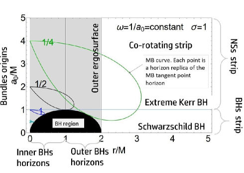
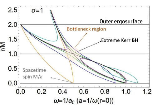
Figure 1: Upper panel: Extended plane $a/M-r/M$ on the equatorial plane $(\sigma=\sin^{2}\theta=1)$ of the Kerr geometry. Metric bundles (MBs) with characteristic frequency $\omega=1/a_{0}=$constant are shown for different values of $\omega$, where $a_{0}$ is the bundle origin spin (bundles value at $r=0$). The black region represents the BH region with the outer and inner horizons $a_{\pm}$, as functions of $r/M$. A horizontal line on the extended plane at $\sigma=1$ represents a fixed spacetime $a/M=$constant. In particular, $a=0$ corresponds to the Schwarzschild BH spacetime and $a=M$ to the extreme Kerr BH. Naked singularities correspond to values $a>M$. The extended plane is shown for co-rotating orbits, i.e., for $a_{0}\geq 0$ and $\omega\geq 0$. The frequencies of the inner and outer horizons curve are clearly distinguished. The frequency $\omega^{\pm}_{H}=1/2$ corresponds to the extreme Kerr BH. On the equatorial plane, the point $r=2M$ is the outer ergosurface (the Schwarzschild BH horizon for $a=0$). Lower panel: Light surfaces $r_{s}^{\pm}(\omega;a)$ on the equatorial plane, solutions of condition $\mathcal{L}_{\mathcal{N}}=0$, as functions of the frequency $\omega$, for different spacetimes. Here, $\omega=1/a_{0}$ corresponds to $r=0$. The extreme BH spacetime and the bottleneck region are also pointed out.

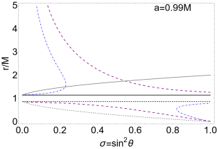
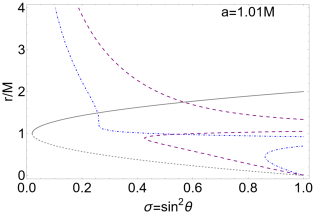
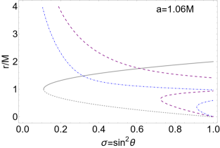
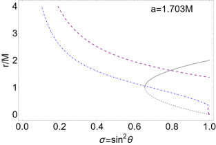
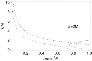
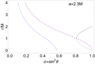
Figure 2: Co-rotating replicas in the Kerr geometry with dimensionless spin $a/M$. Panels show the replicas radius $r$ on each plane $\sigma\equiv\sin^{2}\theta\in[0,1]$ for the BH with spin $a=0.99M$ in the BH spacetime (upper left panel) and in different NSs spacetimes with spin $a/M$ signed on the panels. Lower right panel is a close-up view of the lower left panel. Gray solid (dashed) curve is the outer (inner) ergosphere $r_{\epsilon}^{+}(\sigma)$ ($r_{\epsilon}^{-}(\sigma)$). Purple large-dashed (blue dotted-dashed) curves are the outer (inner) horizons co-rotating replicas for the BH with spin $a=0.99M$. See also Figs (3) and Figs (4).

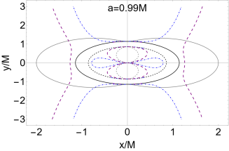
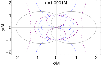
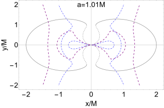
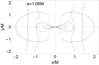
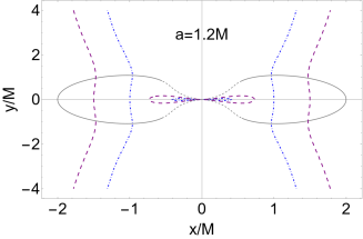
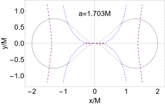
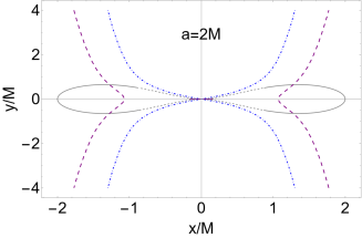
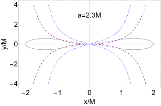
Figure 3: Co-rotating replicas of the BH horizons represented in Fig. (2) for different values of $a/M$ corresponding to BH s with spin $a=0.99M$ and NSs with different spin–mass rations $a/M$ as signed on the panels. Gray solid (dashed) curve is the outer (inner) ergosurface. Black solid (dashed) is the outer (inner) BH horizon. Purple large-dashed (blue dotted-dashed) curve is the outer (inner) BH horizon co-rotating replica. (Here $x=r\sin\theta$ and $y=r\cos\theta$). See also Figs (2) and Figs (4).

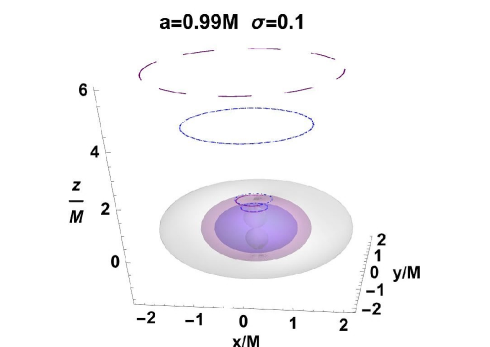
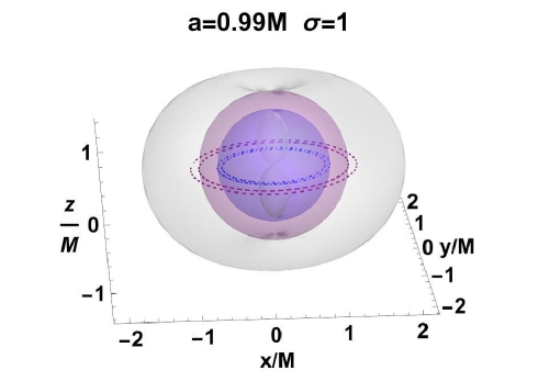
Figure 4: Co-rotating replicas of the BH horizons represented in Fig. (2) for the BH with spin $a/M=0.99$ on the plane $\sigma=0.1$ (with $\sigma\equiv\sin^{2}\theta\in[0,1]$)–upper panel– and on the equatorial plane $\sigma=1$–lower panel. Purple large-dashed (blue dotted-dashed) curve is the outer (inner) BH horizon co-rotating replicas. Here, $\{z=r\cos\theta,y=r\sin\theta\sin\phi,x=r\sin\theta\cos\phi\}$. The central singularity is the point $(x=0,y=0,z=0)$. Gray surfaces are the outer and inner ergosurfaces. Blue surface is the inner horizon, purple surface is the outer horizon. See also Figs (2) and Figs (4).

0.3.4 MBs characteristics in the Kerr extended plane

Below we list some of the main MBs characteristics in the extended plane. The concept of metric bundles and some of their main features are illustrated in Fig. (1)–upper panel, using the extended plane $a/M-r/M$ of the Kerr geometry on the equatorial plane $(\sigma=\sin^{2}\theta=1)$.

Metric bundles of the Kerr spacetimes are solutions of $\mathbf{\mathcal{L_{N}}}=0$, expressed as functions of $(\omega,r,\sigma)$ and can be represented as curves of a plane $a-r$ or $\mathcal{A}-r$ (extended plane), where $\mathcal{A}\equiv a\sqrt{\sigma}$ is the origin spin for any plane $\sigma$–remnants ; bundle-EPJC-complete ; LQG . Figs (1)–upper panel represents the extended plane of the Kerr geometry for $\sigma=1$, where the Kerr bundle curves can be represented through the (dimensionless) spin-function:

$$a(r,\omega)=\frac{2\omega\pm\sqrt{r^{2}\omega^{2}\left[1-r(r+2)\omega^{2}\right]}}{(r+1)\omega^{2}}.$$ (6)

The black region is the BH region bounded by the outer $(r=r_{+}\in[M,2M])$ and inner $(r=r_{-}\in]0,M])$ horizons curves $a_{\pm}\in[0,M]$ of the extended plane $a-r$. Bundles are not defined in the region $]r_{-},r_{+}[$ of BH spacetimes, but they are defined in the BH region $r\in[0,r_{-}]$ and in $r\in[0,2M]$ of NS. The point $(a=0,r=0)$ is the singularity, $(a=M,r=M)$, the maximum of the curve $a_{\pm}$, is the horizon of the extreme Kerr BH, $(a=0,r=2M)$ is the horizon of the Schwarzschild BH . The radius $r=2M$ in the extended plane coincides also with the outer ergosurface on the equatorial plane of all the Kerr BHs and NSs. Each line $a_{\pm}=$constant in this extended plane is a BH geometry. In particular $a=0$ to the Schwarzchild geometry and the zero MBs. Per definition the bundle characteristic frequency $\omega$ is constant along the MBs curve, in particular, the frequency of the origin $r=0$ coincides with the bundle frequency $\omega$.

At a point $r$, in general, there are two different limiting photon frequencies $\omega_{\pm}$ for the stationary observers; then, it follows that at each point of the extended plane (at fixed $\sigma$ and with the exception of the horizon curve) there have to be a maximum of two different crossing metric bundles.

Each MB curve is tangent to the horizon curves in the extended plane at one point only, defining, therefore, uniquely the BH with the MB frequency $\omega$, coinciding with the frequency of the horizon at the point where the bundle is tangent to the horizon curve. The fact that metric bundles are tangent to the horizons curve in the extended plane has significant implications.

The tangent point distinguishes the tangent spin $a=a_{g}\in[0,M]$, on the curve $a_{\pm}$, but it is defined by the tangent radius $r_{g}\in[0,M]$ on inner horizons curve or $r_{g}\in[M,2M]$ on the outer horizon curve. The horizon curve emerge as the envelope surface of all MBs.

Bundles can contain either only BHs or BHs and NSs. In the extended plane, NSs are “necessary” for the construction of horizons curve. The outer horizons curve emerges as envelope surface of bundles with origin in NSs. Part of the inner horizons curve (on the equatorial plane) emerges from MBs with origin in the slowly spinning NSs. Bottlenecks in these NSs spacetimes coincide in the extended plane with the region where these MBs curves are defined. Killing bottlenecks appear in the NSs region of the extended plane containing parts of the MBs tangent to the inner horizons. (The light surface $r_{s}(\omega):\mathcal{L}_{\mathcal{N}}=0$ emerge as the collections of all points, crossing of the MB curve with a line $a=$constant on the extended plane.)

MB curves in the extended plane connect points of different (BH or BH and NS) geometries having all the same characteristic null frequency $\omega$, which is the replica of a BH horizon. Fig. (1) shows metric bundles at $\sigma=1$ for different characteristic frequencies $\omega=1/a_{0}=$constant, where $a_{0}$ is the bundle origin on the plane $\sigma=1$ (corresponding to the solution $a=a_{0}:\mathcal{L}_{\mathcal{N}}=0$ for $r=0$ and $\sigma=1$). In general, $\sigma\in]0,1]$, the bundle origin spin is $\mathcal{A}_{0}\equiv 1/\omega\sqrt{\sigma}$.

Replicas

Replicas are light-like (circular) orbits, of NSs as BHs spacetimes having the same frequency as a BH $\omega_{H}^{\pm}$. All the points of a MB curve are the replica of the BH horizon frequency $\omega_{H}^{+}$ or $\omega_{H}^{-}$ of the BH individuated by the tangent point of a MB curve to the horizon curve $(a_{g},r_{g})$. The study of replicas is the study of the MBs curves in the extended plane.

Per definition all orbits of a bundle are a replica of the horizon the bundle is tangent to. More precisely, replicas connect measurements in different spacetimes characterized by the same value of the property $\mathcal{Q}$ function of $\omega$, by connecting the two null vectors, $\mathcal{L}(r_{\star},a_{\star},\sigma_{\star})$ and $\mathcal{L}(r,a,\sigma)$, to $\mathcal{L}(r_{g},a_{g},\sigma_{g})$ where $r_{g}$ is the tangent radius of the MB  to the outer or inner Killing BH horizon and $(\sigma_{g},a_{g})$, $(\sigma_{\star},a_{\star})$ are generally different from $(\sigma,a)$. In some cases, horizons (frequencies) replicas are in the same spacetime ($a=a_{\star}=a_{g}$).

More precisely, the orbital frequency $\omega$ of a photon on a replica coincides with the BH horizon frequency, which is also the bundle characteristic frequency. Although here we restrict our analysis to the co-rotating replicas, i.e. $\omega>0$ as $a>0$, the study of counter-rotating photon circular orbits with frequency $\omega<0$ is possible with MBs in the extended plane $a\in\mathrm{R}$ with $\omega>0$. Notably not all BH frequencies are replicated. There is a confinement, when a horizon frequency is not replicated i.e. there is no replica connected to that frequency.

On the equatorial plane an exact expression of the Kerr inner horizons replicas in a fixed BH spacetime $a$, $r^{-}_{-}:\quad\omega_{-}(r_{-}^{-})=\omega_{-}(r_{-})=\omega_{H}^{-}$ and outer horizons replicas $r_{+}^{+}:\quad\omega_{+}(r_{+}^{+})=\omega_{+}(r_{+})=\omega_{H}^{+}$ are

$$r^{\mp}_{\mp}=\frac{1}{2}\left(\sqrt{\frac{32r_{\mp}}{a^{2}}-a^{2}\pm 6\sqrt{1-a^{2}}-22}-r_{\mp}\right).$$ (7)

Since $0<r_{-}^{-}<r_{-}<r_{+}<r_{+}^{+}$ – see Figs (2,3,4)– while the outer horizon replicas can be detected on the equatorial plane, the inner horizon replicas remain confined to the observer.

In the Kerr spacetime, part of the inner horizon frequencies are “confined”. However, importantly for the observational point of view, some replicas of the inner horizons are in the proximity of the BH poles, while confined on different planes $(\sigma<1)$. In nuclear ; GRG-letter , the BH poles $(\sigma\approx 0)$ have been studied for the observation of the photon orbits with MBs characteristic frequency. One of the intriguing applications of MBs in BH physics is the possibility to explore the regions close to the BH rotational axes (poles), where it is possible to measure the Kerr inner horizons replicas–nuclear ; GRG-letter . In Figs (2,3), we show the BH horizons replicas in some NSs spacetimes of the two bundles of the Kerr extended plane $\mathcal{A}_{0}-r$ (at different $\sigma$), defined by the characteristic frequencies $\omega_{H}^{\pm}$, respectively, for the spacetime with $a=0.99M$, hence with tangent equal to the tangent spin $a_{g}=0.99M$, but different tangent radius $r_{g}=r_{\mp}$, corresponding to the inner and outer horizon of the BH with spin $a=0.99M$.

Therefore, replicas in a fixed geometry, allow an observer to detect the horizon frequency on a different orbit. The topology of the MBs curves in the extended plane provides information about the local properties of the spacetime replicated in regions more accessible to observes, which can detect the presence of a replica at the point $(r_{\star},\sigma_{\star})$ of the BH spacetime with spin $a_{\star}$, by measuring the BH horizon frequency $\omega_{H}^{+}(a_{\star})$ or $\omega_{H}^{-}(a_{\star})$ (the outer or inner BH horizon frequency) at the point $(r_{\star},\sigma_{\star})$.

The stationary observers orbital frequency is $\omega\in]\omega_{-},\omega_{+}[$ where one of ($\omega_{-},\omega_{+}$) is the horizon’s frequency $\omega_{H}^{+}$, replicated on a pair of orbits $(r_{+},r_{s}^{*})$, where $r_{s}^{*}$ is a light surface orbit, i.e. $r_{s}^{*}=r_{s}^{+}$ or $r_{s}^{*}=r_{s}^{-}$. The second light-like frequency is the frequency of a horizon in a BH spacetime.

From Figs (3) is it possible to see that, for slow spinning NSs, the inner horizons co-rotating replicas change slowly, increasing the singularity spin-mass ratio. The outermost co-rotating replicas of the outer horizon change slowly, increasing the NSs spin with respect to the outermost horizon replicas. The innermost outer horizon replicas change from very slow spinning NSs (upper right panel), slow spinning NSs and very fast spinning NSs. It is clear the change of the NSs replicas between in the spacetimes of very slow spinning NSs (which is similar to the case of BH spacetimes), slow spinning NSs and faster spinning NSs. For very slow spinning NSs the replicas are very close to the inner and outer horizons (upper right and left panels), describing the NSs bottleneck and horizon remnants.

Horizons curve in the extended plane

The horizon curve $a_{\pm}$, solution of $r_{\pm}=r$, boundary of the BH region in the extended plane, is

$$a_{\pm}\equiv\sharp\sqrt{r(2-r)},\quad(\mbox{where}\quad r\in[0,2])$$ (8)

where $\sharp=\pm$, for the co-rotating $(\omega>0)$ and counter-rotating $(\omega<0)$ orbits, respectively.

Frequencies in the extended plane

Explicitly, the limiting frequencies $\omega_{\pm}:\mathcal{L_{N}}=g(\mathbf{\mathcal{L},\mathcal{L}})=0$ are

$$\omega_{\pm}\equiv\frac{\pm\sqrt{\sigma\Delta\Sigma^{2}}-2ar\sigma}{\sigma\left[a^{2}\sigma\Delta-\left(a^{2}+r^{2}\right)^{2}\right]},\quad\mbox{where}\quad\lim_{r\rightarrow\infty}\omega_{\pm}=0$$ (9)

$$\mbox{and}\quad\lim_{r\rightarrow 0}\omega_{\pm}=\frac{1}{a\sqrt{\sigma}}=\frac{1}{\mathcal{A}_{0}}\equiv\omega_{0},$$

where we introduced the frequency function $\omega_{0}$ expressing the bundle characteristic frequency as frequency at the origin $r=0$. Considering the limiting cases of the static Schwarzschild spacetime and of the faster spinning NSs geometry, we obtain

$$\lim_{a\rightarrow 0}\omega_{\pm}=\mp\frac{(r-2)}{\sqrt{(r-2)r^{3}\sigma}}\quad\mbox{and}\quad\lim_{a\rightarrow\infty}\omega_{\pm}=0.$$ (10)

We can write the frequencies in Eq. (9) as frequencies of the horizon curves in the extended plane as

$$\omega_{H}^{\pm}(r)\equiv\omega_{\pm}(a_{\pm})=\frac{\sqrt{(2-r)r}}{2r}\quad\mbox{where},$$ (11)

$$r\in[0,2]\quad\mbox{and}\quad\lim_{a\to 0}\omega_{H}^{\pm}=0,$$

where $r\in[0,2]$ is the horizons radius in the extended plane. Note that $\omega_{H}^{\pm}=0$ for $r=2$. The characteristic frequency $\omega$ is related to the bundles origin $a_{0}\in[0,+\infty]$ (or $\mathcal{A}_{0}\in[0,+\infty]$), and the radius $r\in[0,2]$ on the horizon curve in the extended plane as follows

$$\omega=\frac{1}{\mathcal{A}_{0}}=\frac{1}{a_{0}\sqrt{\sigma}}=\frac{\sqrt{(2-r)r}}{2r}=\omega_{H}^{\pm}(r)\quad(\mbox{where}\quad r\in[0,2]).$$ (12)

Then, $\omega_{\pm}=1/\sqrt{\sigma}$ for the extreme BH, and $\omega_{\pm}$ has a minimum on the equatorial plane, where it is $\omega_{\pm}=\omega_{0}=M/a$.

Note that the light surfaces $r_{s}^{\pm}$ on the Kerr spacetimes equatorial plane can be written as functions of the frequency $\omega$ and parametrized in terms of the bundle characteristic frequency of the origin point $\omega_{0}$ as follows

$$r_{s}^{-}\equiv\frac{2\beta_{1}\sin\left[\frac{1}{3}\arcsin\beta_{0}\right]}{\sqrt{3}},\quad r_{s}^{+}\equiv\frac{2\beta_{1}\cos\left[\frac{1}{3}\arccos(-\beta_{0})\right]}{\sqrt{3}},$$ (13)

$$\mbox{where}\quad\beta_{1}\equiv\sqrt{\frac{1}{\omega^{2}}-\frac{1}{\omega_{0}^{2}}},\quad\beta_{0}\equiv\frac{3\sqrt{3}\beta_{1}\omega^{2}}{\left(\frac{\omega}{\omega_{0}}+1\right)^{2}}$$

–see Figs (1)–lower panel.

MBs curve origin spin

Conversely, the origin spin $a_{0}$ can be read as

$$a_{0}=\frac{2}{\sqrt{\sigma}}\sqrt{\frac{r}{2-r}}=\pm\frac{1}{\omega\sqrt{\sigma}}\quad(\mbox{where}\quad r\in[0,2]).$$ (14)

MBs curve tangent radius

The MB tangent radius $r_{g}\in[0,2]$ to the horizons curve can be expressed in terms of the frequency $\omega$ and the bundle origin spin as

$$r_{g}(\omega)=\frac{2}{4\omega^{2}+1}=\frac{2\mathcal{A}_{0}^{2}}{\mathcal{A}_{0}^{2}+4}$$ (15)

–Figs (5).

MBs curve tangent spin

The MBs tangent spin reads

$$a_{g}(a_{0})=4\sqrt{\frac{\omega^{2}}{\left(4\omega^{2}+1\right)^{2}}}=\frac{4\mathcal{A}_{0}}{\mathcal{A}_{0}^{2}+4},$$ (16)

–Figs (5).

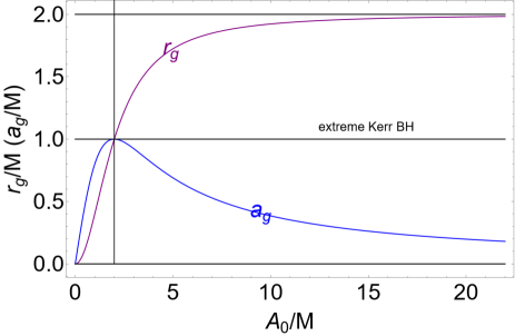
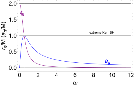
Figure 5: MBs tangent radius $r_{g}$ (purple) and tangent spin $a_{g}$ (blue) as function of the bundle origin spin $\mathcal{A}_{0}\equiv a_{0}\sqrt{\sigma}$. Here we show $\sigma\equiv\sin^{2}\theta\in[0,1]$) (upper panel) and the bundle characteristic frequency $\omega$ (lower panel). See discussion of Sec. (0.3.4). The radius $r_{g}$ is defined in Eq. (15) and tangent spin $a_{g}$ is defined in Eq. (16). The extreme Kerr BH case, for $a_{g}=M$, $r_{g}=M$, $\omega=1/2$, $\mathcal{A}_{0}=2M$ is also shown.

In the next section we shall analyze MBs characteristics for the limits of the KN solution as seen in the extended plane.

0.3.5 Limiting cases

It is possible to explain some MBs properties and their representation in the extended plane by considering some limiting cases, in particular the zeros of the MBs curves in the extended plane. Here, we discuss the limiting cases of the static RN solution and electrically neutral and static limit of the Schwarzschild spacetime.

The definition of the extended plane in the Schwarzschild spacetime is complicated due to the identification of the metric parameter defining MBs. On the other hand, MBs in the Schwarzschild case can be studied as zero limits of the extended planes of the RN and Kerr spacetimes (in the Schwarzschild case, the horizon is the axis $r=2M$ on the Kerr extended plane shown in Figs (1)–left panel.). More generally in static geometries, the bundle characteristic frequencies, solutions of $\mathcal{L}_{\mathcal{N}}=0$, are null and the tangency condition of the metric bundles with respect to the horizons curves is to be understood as an asymptotic condition. In this situation, the horizon replicas are the asymptotic solutions for orbits far from the gravitational source.

Below, first we analyze Schwarzschild MBs as the zeros of the extended planes. Then, we shall discuss the Schwarzschild MBs as limits of the RN MBs, concluding this section with the analysis of the Schwarzschild MBs as limits of the Kerr MBs.

The Schwarzschild MBs as zeros in the extended planes

The Schwarzschild metric case corresponds to the zeros of the metric bundles of the Kerr and RN spacetimes (solutions with $a=0$ and $Q=0$, respectively). The Schwarzschild limiting photon orbital frequencies are

$$\omega=\pm\frac{\sqrt{r-2}}{r^{3/2}\sqrt{\sigma}},$$ (17)

where $\omega=0$ on the BH horizon ($r_{+}=2$).

The Schwarzschild MBs as limits of RN MBs

Let first discuss the RN case, where the horizons are represented as the curve $Q_{\pm}=\sqrt{r(2-r)}$ in the extended plane $Q-r$. Let us consider the Killing field $\mathcal{L}$ and the quantity $\mathcal{L}_{\mathcal{N}}$:

$$\mathcal{L}^{a}\equiv\xi_{(t)}^{a}+\omega\xi_{(\phi)}^{a}\quad\mathcal{L}_{\mathcal{N}}\equiv{g}(\mathcal{L},\mathcal{L})=g_{tt}+g_{\phi\phi}\omega^{2}.$$ (18)

From the equation $\mathcal{L}_{\mathcal{N}}=0$, we find the limiting (photon orbital) frequencies $\omega_{\pm}$ for the RN geometry:

$$\omega_{\pm}=\pm\frac{-g_{tt}}{g_{\phi\phi}}={\pm}\frac{\sqrt{Q^{2}+(r-2)r}}{\sqrt{\sigma}r^{2}}$$ (19)

where $\omega_{\pm}=0$ on $r_{\pm}$. Differently from the Kerr case given in Eq. (9), the frequencies functions in Eq. (19) are even in the electric charge parameter $Q$. In a static spacetime, we can define relatively counter-rotating photon orbits and following the same procedure in the spherically symmetric background, the expression of the MBs in the RN spacetime reflects this property. RN MBs in the extended plane can be represented as the function

$$Q(r)\equiv\sqrt{r}\sqrt{r^{3}\sigma\omega^{2}-r+2}.$$ (20)

The Schwarzschild MBs as limits of the Kerr MBs

Metric bundles of the Schwarzschild geometry are the limiting case of the metric bundles of the Kerr geometry for $a=0$. In this case, $\omega=0$ on the horizon. From Eqs (15), (14) and (16), we obtain

$$\lim_{\omega\to 0}r_{g}(\omega)=2,\quad\lim_{\omega\to 0}a_{0}=\infty\quad\mbox{and}\quad\lim_{a_{0}\to\infty}a_{g}=0.$$ (21)

The first and second limits define the static case for the null horizon frequency $\omega=0$, described as a limiting situation occurring for the horizon tangent point $r_{g}=2$ (the Schwarzschild horizon radius), corresponding to the zero of the (outer) horizon curves in the Kerr extended plane. The frequency $\omega=0$ corresponds also to the MBs origin spin $a_{0}$ for extremely fast spinning NSs. The MBs in the limiting case of very slowly spinning BHs have origins corresponding to extreme fast spinning NSs, as it is clear from the third limit.

0.4 Black hole thermodynamics

Israel’s theorem concerns the uniqueness of the Schwarzschild BH (the only static and asymptotically flat vacuum spacetime with a regular horizon is the Schwarzschild solution) and establishes that the event horizon must be spherically symmetric, implying that the sphericity of an isolated and static BH cannot be broken Israel1 ; Israel2 and HE ; H72152 . This is the first version of the so called “no-hair theorem”, later formulated by Wheeler, and which today refers more generally to a set of theorems and conjectures. The first result of Israel established the uniqueness of the Schwarzschild metric, which was then extended to the case of spinning and charged BHs Carterspinning ; Robinson . Although some steps have been made towards a full generalization of the Israel theorem, there is still no proof for a general no-hair theorem remaining, therefore, a conjecture.

The “no–hair theorem” states also what is known as the simplicity of the isolated BHs in equilibrium, which (in General Relativity) can be fully characterized by the mass $M$, the angular momentum $J$, and the electric charge $Q$. Said differently, all stationary BH solutions of the Einstein–Maxwell equations are defined by only three independent (classical and observable) parameters. The term “hairs” refers to any further “information” as, for example, the matter of the BH progenitor or other “conserved numbers” of the matter swallowed by the BH, which could not be traced back by a far away observer. Hence, the physical BH (as final result of a physical process in a progenitor lifetime) after collapse has left with no other defining (independent) “remnant” parameters, when the matter-field information (prior horizon formation /crossing) “disappeared” behind the BH horizon, inaccessible to the outside observer and, therefore, lost to the observer’s universe.

Hairs, in other words, are fields (different from the electromagnetic ones) and matter, which is associated to and determines stationary BHs.

The conjecture also outlines the BH information paradox (problem) in its classical and quantum formulation, when considering the possible quantum effects associated to the BH and the spacetime close to the horizons. This and the approximation of the general formulation of the conjecture has led to several reformulations, revisions, and modifications to the initial conjecture, as confirmations or exceptions were encountered in relation to specific “hairs–fields” soft1 ; soft2 ; soft3 .

In the first theorem formulation, the electromagnetic field was singled out (excluding, however, a magnetic charge), and excluding further “degrees of freedom” as the Baryon number, for example, or other quantum numbers (as strangeness, etc), which, therefore, could not be measured by a (far away) observer, being destroyed during the collapse (or crossing the horizon).

Therefore, the theorem had the further issue to isolate, without physical foundation, the electromagnetic field (gauge fields subjected to Gaussian law ) with respect to other fields. Several counter–examples have been found with fields hairs for stationary and stable BH solutions. There are stationary BHs with hairs as exterior fields constituting exceptions. Stable stationary BHs solutions with gauge field hair are also known (the BH pierced by cosmic strings are another example of hair as other solutions in non-abelian gauge theories.).

Remarkably, there is no clear, univocal and physically supported indication (or criterion) on the fields to consider as possible BH – “hairs”, this constituting a deeper and broader issue in the “no-hairs” theorem investigation. It should be noted that mass, electric charge and angular momentum are all conserved quantities holding the Gauss law. An eventual magnetic charge, according to this requirement, would be a “proper ” BH hair. However, many BH solutions with gauge fields (different from the Maxwell fields), subjected to a Gauss law were also found.

Therefore, the formulation of a no-hair theorem itself is under scrutiny, so that more than one theorem is to be proved; it resulted into an idea to be tested on a case-by-case basis which, with negative results, confirms the conjecture for that specific case, or provides a counter-examples by narrowing the field of analysis on a possible geometric justification of the BH hair fields, giving raise to a sequence of “no–hair theorems” (there are, for example, non scalar–hair theorem, etc). It would, therefore, be more correct to say that, in the context of General Relativity, the no-hair theorem refers to a series of statements concerning the “degrees of freedom” defining a BH and observable to a distant observer. Another issue of the no-hair theorem is the role of conditions at infinity (and the asymptotic flatness), relevant, for example, in cosmological models, where formulations are known for positive cosmological constant–see BaPRL . Obviously a no-hair theorem would imply the BH “simplicity” and would have consequences on the BH uniqueness. A conceptual consequence of the no–hair theorems (BH simplicity) is that in this way the BH entropy, defined by the BH area, would provide the “real” measure of the BH degrees of freedom. However, the information on the BH “past” (with respect to the state of observation), in the sense of BH “hair”, is to be considered eliminated or inaccessible to far away observers.

This field of investigation with its problematic aspects is a promising cross-road among BH physics, quantum gravity, information theory, and theories of great unification. Nevertheless, this relevant aspect of BH physics diverges from the purposes of this chapter and we refer the reader, for further details on this issue, to the extensive literature on the subject.

Here we explore the laws of BH thermodynamics in the extended plane, using the Smarr’s formula connecting, in the Kerr BH spacetime, $(M,J,A_{area})$, where $A_{area}$ is the (outer) BH horizon area Smarr . The extended plane and MBs can be used to relate different states of a BH, interacting with its environment. Replicas can connect BH spacetimes related in a transition and governed by the thermodynamic laws in the extended plane. Hence, it is possible to reformulate BH thermodynamics in terms of the light surfaces, exploring the thermodynamic properties of the geometries through the metric bundles.

This formalism turns out to be adapted to the description of the BH state transitions, constrained by the properties of the null vector $\mathcal{L}$, building up many of the thermodynamic properties of BHs, as it enters the definitions of thermodynamic variables and stationary observers.

In this section, we detail the BH thermodynamic properties in terms of the null vector $\mathcal{L}$ and, therefore, of the metric bundles. Sec. (0.4.1) discusses the role of metric bundles and the quantity $\mathcal{L_{\mathcal{N}}}$ in BH thermodynamics, introducing the concept of BH surface gravity, the first law of BH thermodynamics, and concluding with some notes on the BHs states transitions as described by the laws of BH thermodynamics.

In this framework, we explore BH states transition in the extended plane in Sec. (0.4.2). The BH irreducible mass is the subject of Sec. (0.4.3), where we discuss also the extraction of BH rotational energy as constrained with MBs. Finally, Sec. (0.4.4), BH thermodynamics in the extended plane, closes this section.

0.4.1 Black hole thermodynamics, metric bundles and the quantity $\mathcal{L_{\mathcal{N}}}$

In this section, we discuss some concepts of BH thermodynamics in terms of metric bundles and the quantity $\mathcal{L_{\mathcal{N}}}$. First, we introduce the concept of BH surface gravity, we then discuss the first law of BH thermodynamics, concluding the section with some notes on the BHs states transitions.

BH surface gravity

We start our analysis of the BH thermodynamics by introducing the concept of BH surface gravity and derive a surface gravity function in the extended plane, expressed in terms of MBs characteristics.

The surface gravity $\ell$ for a BH Killing horizon is defined by the fact that the Killing vector defines a non-affinely parametrized geodesic on the Killing horizon (a global Killing vector field $\mathcal{L}^{a}$ becomes null on the event horizon). According to the Zeroth Law of BH thermodynamic, the surface gravity of a stationary BH is constant over the event horizon (somehow fixing a concept of BH thermal equilibrium)– see for example WW .

In general terms, given an object and its surface, we can define the surface gravity as the (gravitational) acceleration a test particle in the proximity of the object is subject to. Then, a BH surface gravity is the acceleration, as exerted at infinity, of a test particle located in close proximity to the BH outer horizon, which is necessary to keep it at the horizon. For a static BH, it can be expressed as the force exerted at infinity to hold a test particle at close proximity of the horizon. Notice that the locally exerted force at the horizon is infinite.

A similar definition holds for stationary BHs and, in general, for BHs with “well defined” Killing horizons. However, surface gravity is a classical geometrical concept, playing a major role in BH thermodynamics–BCH . Bekenstein first suggested the analogy leading to the concepts of BH entropy and temperature and the formulation of classical BH thermodynamics–Bekenstein73 ; Bekenstein75 .

Hawking later confirmed Bekenstein’s conjecture of a reliability of a BH entropy definition, establishing the (correct) constant of proportionality relating the BH entropy and BH area, following a more complex and complete argument relating BH thermodynamics and BH energy extraction Hawking75 ; H77 ; SV96 .

The introduction of a temperature leads naturally to inquire about a possible BH radiation emission, which would be regulated by the temperature defined by its surface gravity. (However, although the BH temperature could be null, the BH entropy could not vanish). An interpretation of this suggestion has been realized in the quantum (semi-classical) frame. BH thermal radiation has been shown to be the result of quantum mechanical effects governed by the BH temperature and, therefore, its surface gravity (Hawking semi-classical radiation). The surface gravity regulates also the probability of a negative energy particle tunneling through the horizon–Hawking75 . Because it radiates, one can expect the BH mass to decrease and eventually disappear. Nevertheless, the actual fate of the BH and the information carried in the BH during and before the evaporation process, the possible existence of remnant at the end of process, and the entropy evolution are matters of an ongoing (vivacious) debate–see for example JP16 ; LS ; Hawking05 . The actual fate of a BH, following the characteristic thermal emission, is an example of controversial aspects of the surface gravity physics.

Thus, the BH (Bekenstein-Hawking) entropy links gravitation, BH thermodynamics, geometry, and quantum theory. The so-called (BH) information paradox is seen today as the source of one of most promising hints for a quantum theory of gravity.

The relation between area and entropy and the discussion around their constant of proportionality had enormous relevance far beyond the study of BHs. The Bekenstein bound was the starting point, for example, of the holographic principle and in general shred light on profound aspects of geometric theories and problems of quantum information theory.

The history of Bekenstein bound confirmations, developments and applications is broad and complex. As it goes beyond the discussion in this chapter, we refer the interested reader to the extensive literature on the subject. Here, we will reformulate the relation (proportionality) between the concept of entropy and BH area, in terms of light surfaces through the MBs.

Formally, surface gravity may be defined as the rate at which the norm of the Killing vector $\mathcal{L}$ vanishes from outside (i.e. from $r>r_{+}$). In fact, $\ell$ is (the constant) defined through the relation $\nabla^{a}\mathcal{L_{N}}=-2\ell\mathcal{L}^{a}$ (on the outer horizon).

Equivalently, $\mathcal{L}^{b}\nabla_{a}\mathcal{L}_{b}=-\ell\mathcal{L}_{a}$ and $L_{\mathcal{L}}\ell=0$, where $L_{\mathcal{L}}$ is the Lie derivative,-a non affine geodesic equation, i.e., $\ell=$constant on the orbits of $\mathcal{L}$. (The norm $\mathcal{L_{N}}\equiv g(\mathcal{L},\mathcal{L})$ is constant on the horizon.)

For the Kerr spacetime it is $\ell=(r_{+}-r_{-})/2(r_{+}^{2}+a^{2})$. In the extreme Kerr spacetime ($a=M$), where $r_{\pm}=M$, the surface gravity is zero and the BH temperature is also null ($T_{H}=0$), but with a non-vanishing entropy Wald:1999xu ; WW . This relevant fact establishes a profound topological difference between BHs and extreme BHs, implying that a BH cannot reach the extremal limit in a finite number of steps–(third law of BH thermodynamics)– having consequences also regarding the stability against Hawking radiation.

On the other hand, the condition (constancy of ) $\nabla^{a}\mathcal{L}=0$ when $\ell=0$ substantially constitutes the definition of the degenerate Killing horizon BH. In the case of Kerr geometries, only the extreme BH case is degenerate. Therefore, in the extended plane it corresponds to the point ($a=M$, $r=M$). (The BH surface gravity $\ell$, is also a conformal invariant of the metric. Furthermore the surface gravity re-scales with the conformal Killing vector, i.e. it is not the same on all generators but, because of the symmetries, it is constant along one specific generator–see also J-S09 ; Jacobson:2010iu .)

First law of BH thermodynamics

The Kerr BH area is given by the function

$$A_{area}=\int\limits_{0}^{\pi}d\theta\int\limits_{0}^{2\pi}\sqrt{g_{\phi\phi}g_{\theta\theta}}d\phi=4\pi\left(a^{2}+r^{2}\right),$$ (22)

evaluated on the outer horizon $r=r_{+}$. The BH (horizon) area $A_{area}^{+}$ is related to the outer horizon definition, $A_{area}^{+}=8\pi mr_{+}$, where $M=c^{2}m/G=m$ in geometric units. (For simplicity, in some of the expressions we do not consider the factor $8\pi$ and in some expressions we write spin, radius, characteristic frequency and origin spin as dimensionless parameters.)

The BH horizon area is non-decreasing, a property which is considered as the second law of BH thermodynamics (establishing the impossibility to achieve with any physical process a BH state with zero surface gravity). Note that the (Hawking) temperature term is related to the surface gravity by $T^{+}_{H}={\hslash c\ell^{+}}/{2\pi k_{B}}$, while the horizon area $A_{area}^{+}$ defines the BH entropy as $S^{+}=k_{B}A_{area}^{+}/l_{P}^{2}$, $l_{P}$ is the Planck length, $\hslash$ the reduced Planck constant, and $c$ is the speed of light, $k_{B}$ is the Boltzmann constant. (We use the notation $(+)$ or $\mathcal{Q}_{H}^{+}$ for all the quantities $\mathcal{Q}$, evaluated on the outer Killing horizon.)

The first law of BH thermodynamics, $\delta M=(1/8\pi)\ell_{H}^{+}\delta A^{+}_{area}+\omega^{+}_{H}\delta J$, relates the variation of the mass $\delta M$, to the (outer) horizon area $\delta A^{+}_{area}$, and angular momentum $\delta J$ with the surface gravity $\ell_{H}^{+}$ and angular velocity $\omega_{H}^{+}$ on the outer horizon. In this expression, the term $p^{+}=-\omega_{H}^{+}$, could be seen as “pressure-term”, where the internal energy is $U=GM$. The term $\omega_{H}^{+}\delta J$ is interpreted as the “work”. The volume term is $V=GJ/c^{2}$ (where $J=amc^{3}/G$).

We shall consider generalized definitions in the extended plane, where we express some of the concepts of BH thermodynamics in terms of the norm $\mathcal{L}_{\mathcal{N}}$, which defines the metric bundles. It will be necessary to consider quantities evaluated on the inner horizon, where we use the notation $(-)$ or $\mathcal{Q}_{H}^{-}$ for a quantity $\mathcal{Q}$.

BHs transitions

We can describe the BH transition from an initial state $(0)$ to a new state $(1)$ in terms of the characteristic bundle frequency (appearing explicitly in the first law as the work term $\omega^{+}_{H}\delta J$). We use the notation $(0)$ and $(1)$ to indicate any quantity related to the initial and final state, respectively; therefore, $\omega_{H}^{+}(0)$ is the MB frequency tangent to the outer horizon of the BH at the initial state $(0)$. The notation $\delta\mathcal{Q}\equiv\mathcal{Q}(1)-\mathcal{Q}(0)$ denotes the change of the quantity $\mathcal{Q}$ from the initial $(0)$ to the final state $(1)$ of the transition. As in the bundles framework we evaluate quantities in the extended plane, we express many quantities considered here as evaluated on the inner horizons. There is a relation between the quantities $(\delta A_{area}^{-},\delta J,\delta M)$ and $(\omega_{H}^{-}(0),\ell^{-}(0))$ evaluated on the inner horizon $r_{-}$. All the quantities are expressed in terms of bundles at $\omega_{H}^{\pm}(0)=$constant and $(\delta A_{area}^{\pm},\delta J,\delta M)$, describing the transition from the initial to final state.

0.4.2 Masses and BH thermodynamics

We proceed relating the parameters $(\ell^{\pm},\omega^{\pm}_{H})$, regulating the BH transition from one state to another, represented as a transition from a point $r(0)$ to a point $r(1)$ along the horizons curve in the extended plane in the following two cases: 1. $(r(0),r(1))\in[0,1]$, inner horizon range, and 2. $(r(0),r(1))\in[1,2]$, outer horizon range (note, we included the horizon $r_{\pm}=1$ for the extreme Kerr spacetime in both the inner and outer horizons ranges). We will connect properties defined on the outer horizons curve of the extended plane with properties defined on the inner horizons curve of the extended plane.

The frequency $\omega_{H}^{\pm}$ will be considered always positive or null, i.e., $J\omega_{H}^{\pm}\geq 0$, or $a\omega_{H}^{\pm}\geq 0$, vanishing only for $J=a=0$. This implies that we will not consider counter-rotating orbits, nor we shall connect proprieties defined in the positive section of the extended plane to the negative section of the extended plane. However, with $J\omega_{H}^{\pm}\geq 0$, the surface gravity $\ell_{H}^{\pm}$ can be negative, when evaluated on a point of the inner horizon ($\ell_{H}^{-}\leq 0$).

We consider the quantity $s$ such that $\mathcal{P}_{\pm}(r(0))=s\mathcal{P}^{*}_{\pm}(r(1))$, where $\mathcal{P}_{\pm}\in\{\ell_{H}^{\pm},\omega_{H}^{\pm}\}$ and the notation $(*)$ represents an eventual change in sign. Note that $\delta A_{area}^{+}=-\delta A_{area}^{-}$ for $\delta M=0$ (as, per definition, $\delta M^{+}=\delta M^{-}\equiv\delta M$). For a fixed BH spacetime $\delta M^{+}=\delta M^{-}$, but the relation regulating this variation with the other characteristic quantities depends on the point on the horizons curve.

More generally, we can consider $\delta M^{\star}(a(0))=s\delta M^{\ast}(a(1))$, where $(a(0),a(1))\in[0,M]$, $s$ is a constant, and for $a(0)=a(1)$ there is $(\star=\ast=\pm,s=1)$. In general, it can be proved that

$$\delta M^{+}=\ell_{H}^{+}\delta A_{area}^{+}+\omega_{H}^{+}\delta J^{+}=\delta M=$$ (23)

$$\ell_{H}^{+}\delta A_{area}^{+}+\omega_{H}^{+}\delta J=\delta M^{-}\equiv\ell_{H}^{-}\delta A_{area}^{-}+\omega_{H}^{-}\delta J^{-}.$$

Assuming $s\geq 0$ and $s\neq 1$, we consider the relations $\omega_{H}^{*}(r(0))=s\omega^{\star}_{H}(r(1))$ and $\ell_{H}^{\circ}(r(0))=-s\ell^{\diamond}_{H}(r(1))$, where $(\circ,\diamond)=\pm$. Note that s $\ell_{H}^{+}(a)\geq 0$ (surface gravity as function of the spin $a$ in the extended plane) and $\ell_{H}^{-}(a)\leq 0$, where $\ell_{H}^{+}(a)<-\ell_{H}^{-}(a)$. Also, $\ell_{H}^{\circ}(s)<0$ for $s\in]0,1[$ and $\ell(r)\gtreqless 0$ for $r\gtreqless 1$ (surface gravity/acceleration as function of the radius $r$ on the extended plane). We obtain a horizon parametrization in terms of the constant $s$, where $r(0)$ and $r(1)$ correspond to the horizons of the BH spacetime with $a(r(0))=a(r(1))$. However, the limiting case $s=1$ corresponds to the extreme Kerr BH. Also, for $s\in]0,1[$ we have that $r(1)=r_{-}(1)$ and $r(0)=r_{+}(0)$, and for $s>1$, it holds $r(1)=r_{+}(1)$ and $r(0)=r_{-}(0)$, where

$$\frac{r(1)}{r(0)}=s,\quad r(1)=\frac{2s}{s+1},\quad\omega(r(1))=\frac{1}{2\sqrt{s}},\quad\ell(r(1))=\frac{s-1}{4s}$$ (24)

$$\mbox{where}\quad a(r(1))=a(r(0))=2\sqrt{\frac{s}{(s+1)^{2}}}$$

($\omega$ is the bundle characteristic frequency). It is noteworthy that the $s$ factor is different according with the spin, i.e., expressed in terms of the spin it is $s=\hat{s}_{\mp}\equiv[({2-a^{2}})\mp 2\sqrt{({1-a^{2}})}]/{a^{2}}$.

0.4.3 The BH irreducible mass

The total BH mass $M$ of the Kerr BH can be decomposed into the mass $M_{irr}$ and the rotational energy. From the first law of BH thermodynamics, we obtain $M^{2}=M_{irr}^{2}+J^{2}/4M_{irr}^{2}$ (note, $J$ has units of mass $M^{2}$ and it is measured in the asymptotic flat region). The Kerr BH irreducible (or rest) mass $M_{irr}=\sqrt{a^{2}+r_{+}^{2}}/2$, where $A_{area}=16\pi M_{irr}^{2}$ (evaluated on the outer horizon). It follows that

$$\frac{M^{+}_{irr}}{M}=+\frac{\sqrt{1+\sqrt{1-\frac{J(0)^{2}}{M(0)^{4}}}}}{\sqrt{2}},$$ (25)

or, more generally the four solutions

$$\frac{M_{irr}}{M}=\flat\frac{\sqrt{1\natural\sqrt{1-(a_{(\pm)})^{2}}}}{\sqrt{2}},\quad\mbox{where}\quad\flat=\mp;\;\natural=\pm.$$ (26)

Here, $a_{(\pm)}$ is the dimensionless spin on the horizons curve, where

$$\frac{M^{+}_{irr}}{M^{-}_{irr}}=\sqrt{\frac{r_{+}}{r_{-}}}=\sqrt{\frac{\omega_{H}^{-}}{\omega_{H}^{+}}}=\sqrt{\frac{-\ell_{H}^{-}}{\ell_{H}^{+}}}=\frac{\sqrt{r_{+}}}{\sqrt{2-r_{+}}}=\sqrt{\frac{1}{4(\omega_{H}^{+})^{2}}}=\frac{\mathcal{A}_{0}}{2},$$ (27)

in terms of the bundles origin spin $\mathcal{A}_{0}\geq 2$. (The notation $\pm$ refers to the radii $r_{\pm}$.) (Note that $M_{irr}/M=\{0,1\}$ for $a=0$ and $M_{irr}/M=\pm 1/\sqrt{2}$ for $a=M$.).

Equations (27) and (26) are in terms of quantities defined on the extended plane where, in terms of the irreducible mass $M_{irr}$, we obtain

$$\mathcal{A}_{0}(all)=\frac{2M_{irr}}{\sqrt{1-M_{irr}^{2}}}.$$ (28)

Here and in the following analysis, for $\mathcal{Q}(all)$ it is intended a generic quantity $\mathcal{Q}$, considering the entire horizon curve in the positive section of the extended plane.

Therefore, the BH irreducible mass can be written as follows:

$$M_{irr}(all)=\sqrt{\frac{\mathcal{A}_{0}^{2}}{\mathcal{A}_{0}^{2}+4}}=\sqrt{\frac{r}{2}}=\sqrt{\frac{1}{4\omega^{2}+1}},$$ (29)

$$\mbox{and}\quad M_{irr}^{\mp}=\sqrt{\frac{1}{2}\mp\frac{1}{2}\sqrt{\frac{\left(\mathcal{A}_{0}^{2}-4\right)^{2}}{\left(\mathcal{A}_{0}^{2}+4\right)^{2}}}}=\sqrt{\frac{r_{\mp}}{2}},$$

–Fig. (6)– ($r$ is a point on the horizon curve in the extended plane).

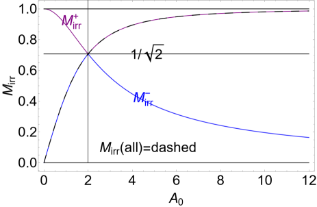
Figure 6: Irreducible mass function $M_{irr}$ versus bundle origin spin $\mathcal{A}_{0}\equiv a_{0}\sqrt{\sigma}$ ($\sigma\equiv\sin^{2}\theta$). The functions $M_{irr}^{\pm}$ and $M_{irr}(all)$ are defined in Eq. (29). The limiting value $M_{irr}^{\pm}=M_{irr}(all)=1/\sqrt{2}$ for $\mathcal{A}_{0}=2$ (corresponding to the extreme Kerr BH ) is also shown. For $\mathcal{A}_{0}>2$ ($\mathcal{A}_{0}<2$) metric bundles are tangent to the outer (inner) horizons curves in the extended plane. See the analysis of Sec. (0.4.3). All quantities are dimensionless.

The dependence on $\sigma$, implicit in the bundle origin definition $\mathcal{A}_{0}\equiv a\sqrt{\sigma}$, does not contradict the BH horizon rigidity, as it has to be considered as a representation of the light surfaces frequencies on different poloidal angle $\sigma$s. In Eq. (29), we note the special value $\mathcal{A}_{0}=2$, corresponding to a bundle characteristic frequency $\omega=1/2$, tangent to the horizon curve point, corresponding to the extreme Kerr BH $(r=r_{\pm}=1)$, where $M_{irr}=1/\sqrt{2}$.

In terms of the bundle origin spin, we obtain the limiting values,

$$\lim_{\mathcal{A}_{0}\to\mathbf{X}}M_{irr}(all)=\left\{1,0,\frac{1}{\sqrt{5}},\frac{1}{\sqrt{2}}\right\},\quad\mbox{and}$$ (30)

$$\lim_{\mathcal{A}_{0}\to\mathbf{X}}M_{irr}(r_{+})=\left\{1,1,\frac{2}{\sqrt{5}},\frac{1}{\sqrt{2}}\right\}$$

for $\mathbf{X}=\{+\infty,0,1,2\}$, respectively.

The rotational energy $\xi$

The upper limit of the the amount of energy that can be extracted from a Kerr BH is the total rotational energy, occurring when the Kerr BH final state is a Schwarzschild BH Ruffini . The total mass $M$ at the end of a (stationary) process of the energy extraction has to be with $M_{irr}$, which is the maximum rotational energy that can be extracted from the black hole is $\xi\propto(M-M_{irr})$. Hence, the maximum rotational energy which can be extracted is the limit of $\xi=\xi_{\ell}\equiv\left(2-\sqrt{2}\right)/2$, where at the state $(0)$ (prior to the extraction) there is an extreme Kerr spacetime (with spin $a=M$). In general, $\xi\in[0,\xi_{\ell}]$.

The extracted rotational energy $\xi$ is

$$\frac{\xi}{M(0)}=1-\frac{\sqrt{1+\sqrt{1-\frac{J(0)^{2}}{M(0)^{4}}}}}{\sqrt{2}}.$$

In the extended plane, we can express the tangent (dimensionless) spin as function of the rotational energy parameter $\xi$:

$$a_{\xi}(\xi)\equiv 2\sqrt{(2-\xi)(\xi-1)^{2}\xi},$$ (31)

linking the former state spin $a(0)$ to the rotational extraction in the subsequent phase, where the BH is settled in a Schwarzschild spacetime. More generally, solving $a_{\xi}(\xi)\equiv a_{(\pm)}$ for $\xi$, we obtain the four solutions

$$\xi_{s}^{(\pm)}=1\flat\frac{\sqrt{1\natural\sqrt{1-a_{(\pm)}^{2}}}}{\sqrt{2}},\quad\mbox{where}\quad\flat=\mp;\quad\natural=\pm,$$ (32)

where $a_{(\pm)}$ is the dimensionless spin on the horizons curve.

The dimensionless spin $a/M\equiv J(0)/M(0)^{2}$ refers to an initial state before the transition, defined by the mass $M(0)$ and spin $J(0)$, function of the extracted rotational energy $\xi/M(0)=1-M_{irr}(0)/M(0)$, and, therefore, of the ratio $M_{irr}(0)/M(0)$. Measuring $\xi$, therefore, will provide and indication of the BH spinDaly0 ; Daly2 ; Daly3 ; GarofaloEvans ; ella-correlation , relating the dimensionless BH spin $a/M$ to the dimensionless ratio $\xi$ (as total released rotational energy versus BH mass, measured by an observer at infinity, and assuming a process ending with the total extraction of the rotational energy of the central Kerr BH).

We have that $a_{\xi}(\xi)\in[0,M]$ (dimensionless) with $\xi\in[0,\xi_{\ell}]$, limiting, therefore, the (rotational) energy extracted (through a classical process) to a maximum of $\approx 29\%$ of the mass $M$. More in details: $\xi=1$ for $a_{\xi}({\xi})=0$ (the static limit corresponds also to the values $\xi=\{0,2\}$). For the extreme case, where $a=M$ and the frequency is $\omega=1/2$, it is $\xi=1\pm{1}/{\sqrt{2}}$. There is a maximum $\xi_{\ell}\equiv\left(2-\sqrt{2}\right)/2$ (and $\xi_{m}\equiv\left(2+\sqrt{2}\right)/2$), where $a_{\xi}(\xi)=M$ and $r_{+}=M$ (the extreme Kerr BH).

We can relate the rotational energy parameter $\xi$ to the horizons, in the extension of the plane for extended values of $\xi$, where the following two cases are possible

$$\mathbf{(1)}\quad\xi^{\mp}_{\pm}=1\pm\sqrt{\frac{r_{\mp}}{2}},\quad\mbox{and}\quad\xi_{\nu}^{\mp}\equiv 1\mp\sqrt{\frac{r}{2}},\quad\mbox{then}\quad\xi_{\tau}^{\mp}\equiv 1\mp\frac{1}{\sqrt{4\omega^{2}+1}},$$

$$\mathbf{(2)}\quad\xi_{\mu}^{\mp}=1\mp\sqrt{1-\frac{r}{2}},\quad\mbox{then}\quad\xi_{\tau\tau}^{\mp}\equiv 1\mp\frac{2\omega}{\sqrt{4\omega^{2}+1}}$$ (33)

–Figs (7). Here, $r$ is a point of the horizon curve in the extended plane. However, as $\xi\propto M-M_{irr}$ the solution $\xi_{-}^{+}$ has to be considered.

Within this parametrization, the frequency $\omega_{H}^{+}={1}/{2\sqrt{2}}$ for the outer horizon $r/M=4/3$ (BH with dimensionless spin $a/M={2\sqrt{2}}/{3}$) is also the saddle point of $\xi_{\tau}^{\pm}$ as function of $\omega$. The maximum extractable rotational energy decreases/increases faster with the horizon (and MBs) frequencies constrained by the limiting values $\omega_{H}^{+}={1}/{2\sqrt{2}}$.

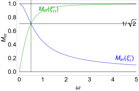
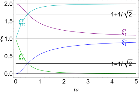
Figure 7: Black hole irreducible mass functions $M_{irr}$ (upper panel) and maximum extractable rotational energy $\xi$ (lower panel) versus bundle characteristic frequency $\omega$. See the analysis of Sec. (0.4.3). The functions $\xi_{\tau}^{\pm}$ and $\xi_{\tau\tau}^{\pm}$ are in Eq. (33), with limiting values $\xi_{\tau}^{+}=\xi_{\tau\tau}^{+}=1+1/\sqrt{2}$ and $\xi_{\tau}^{-}=\xi_{\tau\tau}^{-}=1-1/\sqrt{2}$ for $\omega=1/2$ (corresponding to the extreme Kerr BH ) are also shown. The functions $M_{irr}(\xi_{\tau}^{-})$ and $M_{irr}(\xi_{\tau\tau}^{-})$ are in Eq. (35). The limiting value $M_{irr}(\xi_{\tau}^{-})=M_{irr}(\xi_{\tau\tau}^{-})=1/\sqrt{2}$ for $\omega=1/2$ (corresponding to the extreme BH ) is shown. All quantities are dimensionless.

The characteristic bundle (horizons) frequencies, can be expressed in terms of the dimensionless parameter $\xi$ as

$$\omega_{\pm}\equiv\frac{1\pm\sqrt{4(\xi-2)\xi(\xi-1)^{2}+1}}{4\sqrt{(2-\xi)(\xi-1)^{2}\xi}}.$$ (34)

With the irreducible mass definitions and Eqs (33) we obtain, respectively

$$\mathbf{(1)}\quad\frac{M_{irr}}{M}=1-\xi^{\mp}_{\pm}=\mp\sqrt{\frac{r_{\mp}}{2}},\quad\mbox{where}\quad\frac{M_{irr}(\xi_{\nu}^{\mp})}{M}\equiv 1-\xi_{\nu}^{\mp}=\pm\sqrt{\frac{r}{2}}$$

$$\mbox{and}\quad\frac{M_{irr}(\xi_{\tau}^{\mp})}{M}\equiv 1-\xi_{\tau}^{\mp}=\pm\frac{1}{\sqrt{4\omega^{2}+1}}$$

$$\mathbf{(2)}\quad\frac{M_{irr}(\xi_{\mu}^{\mp})}{M}\equiv 1-\xi_{\mu}^{\mp}\equiv\pm\sqrt{1-\frac{r}{2}},$$ (35)

$$\mbox{and}\quad\frac{M_{irr}(\xi_{\tau\tau}^{\mp})}{M}\equiv 1-\xi_{\tau\tau}^{\mp}=\pm\frac{2\omega}{\sqrt{4\omega^{2}+1}}$$

–Figs (7). For $r=0$, according to Eqs (33), it is $M_{irr}/M=\{1,0\}$, with $M_{irr}/M=1/\sqrt{2}$ for $r=M$, and $M_{irr}/M=0$ for $r=2M$.

0.4.4 BH thermodynamics in the extended plane

Let us start from the relation

$$\frac{\delta M_{irr}}{M_{irr}}=\frac{\delta M-\delta J\omega_{H}^{+}(0)}{\sqrt{M(0)^{2}-\frac{J(0)^{2}}{M(0)^{2}}}},$$

where $\delta M_{irr}\geq 0$, thus $(\delta M-\delta J\omega_{H}^{+}(0))\geq 0$ and all quantities are evaluated on the outer Killing horizon for the initial BH.

Note, the upper bound $\delta M_{irr}\geq 0$ sets the limit

$$\frac{\delta J}{\delta M}\leq\frac{1}{\omega^{+}_{H}(0)}=\mathcal{A}_{0}(0)=\frac{2r(0)}{\sqrt{(2-r(0))r(0)}}$$

$$(\mbox{where}\quad\mathcal{A}_{0}(0)\geq 2,\quad r(0)\in[1,2])$$ (36)

to any spin variation of the BH , where we have used Eq. (12) in terms of the dimensionless origin spin of the bundle and its dimensionless tangent radius to the outer horizon curve. It is a well known fact that limits of BH energy extraction are imposed by the BH horizon. Indeed, massive particles or photons with momentum $p^{a}$ that cross the outer horizon $r_{+}$ of a Kerr BH should satisfy the inequality $-p_{a}(\mathcal{L}_{H}^{+})^{a}\geq 0$, This implies that $\mathcal{E}-\omega_{H}^{+}\mathcal{L}\geq 0$, for $\mathcal{E}\equiv-p_{a}\xi^{a}_{(t)}$ (energy of the particle as measured at infinity), where $\mathcal{L}=p_{a}\xi^{a}_{(\phi)}$ is the $\phi$ component of the particle (photon) angular momentum. Thus, the specific angular momentum $\mathcal{L}/\mathcal{E}\leq 1/\omega_{H}^{+}=\mathcal{A}_{0}$. If the energy $\mathcal{E}$ is negative, $\mathcal{L}$ is negative and the BH spin is reduced (BH spin–down). (The bound regulates also the super-irradiance as the analogue of the Penrose process for radiation scattering by a Kerr BH. For a wave–mode of angular-frequency $\omega$, $\omega$ is amplified if $\omega\in]0,{z}/{\mathcal{A}_{0}}[$, where $z\in Z-\{0\}$ is the wave angular momentum number).

More generally, the BH area is a function of the horizon radius as $A_{area}(a_{\pm})=8\pi r$. Considering the variation of the horizon area (and the irreducible masses) for the ADM mass $M$, the area $A_{area}$ and the momentum $J$, we obtain

$$\delta M^{\mp}=\frac{\ell^{\mp}}{8\pi}\delta A_{area}^{\mp}+\omega_{H}^{\mp}\delta J^{\mp},$$ (37)

where the following relation holds

$$\frac{da_{\pm}}{dr}=\mp\left.\frac{\ell}{\omega_{\pm}}\right|_{a=a_{\pm}},$$ (38)

in terms of frequency and surface gravity function evaluated on the horizon curve $a_{\pm}$.

Explicitly, using the expressions for the bundle frequencies and the surface gravity function,

$$\omega=\frac{\sqrt{2-r}}{2\sqrt{r}}=\frac{1}{2}\sqrt{1-4\ell},\quad\mbox{and}\quad\ell(r,a_{\pm})=\frac{r-1}{2r},$$

which are related by $\ell=\omega_{\mathbf{EBH}}^{2}-\omega^{2}$, where $\omega_{\mathbf{EBH}}=1/2$ is the extreme BH horizon frequency.

Finally, in the extended plane, we obtain

$$\delta M=\frac{\delta A_{area}(r-1)}{2r}+\frac{\delta J\sqrt{2-r}}{2\sqrt{r}},\quad\mbox{and}$$ (39)

$$\delta M=\delta A_{area}\left(\frac{1}{4}-\omega^{2}\right)+\delta J\omega,\quad\mbox{or}\quad\delta M=\left(\frac{1}{4}-\frac{1}{\mathcal{A}_{0}^{2}}\right)\delta A_{area}+\frac{\delta J}{\mathcal{A}_{0}}$$

in terms of the MBs tangent radius $r$, characteristic frequency $\omega$, and origin spin $\mathcal{A}_{0}$, where the limiting case $\mathcal{A}_{0}=2$, $\omega=1/2$ and $r=1$ corresponds here to the extreme Kerr BH , distinguishing the relations defined on the inner and outer horizons curves in the extended plane, where the terms relative to the surface gravity change sign.

From $A_{area}^{-}=-A_{area}^{+}+4M^{2}$, we can write $\delta A_{area}^{-}=-\delta A_{area}^{+}+8M\delta M$, (with $\delta J=0$ then $\delta M={\delta A_{area}^{+}\ell_{H}^{+}}/{2M}$).

In the special case of $\delta M=0$ (invariant BH mass), $\delta A^{+}_{area}=-\delta A_{area}^{-}$ and

$$\frac{\delta J}{\delta A_{area}^{+}}=\frac{\ell^{-}+\ell^{+}}{\omega_{H}^{-}-\omega_{H}^{+}}.$$ (40)

Then, using quantities as defined in the extended plane, we obtain

$$\frac{\delta J}{\delta A_{area}^{\mp}}=(\pm)\frac{\sqrt{1-a^{2}}}{a}=\frac{4-\mathcal{A}_{0}^{2}}{4\mathcal{A}_{0}}=\frac{4\omega^{2}-1}{4\omega}=\frac{1-r}{\sqrt{r(2-r)}},$$ (41)

which represents the variation of the angular momentum versus area in terms of the initial bundle tangent point of the horizon $(a,r)$, or, alternately, the characteristic frequency $\omega$ or its origin spin $\mathcal{A}_{0}$ in dependence from the poloidal angle $\sigma$. Note that the limiting case $\mathcal{A}_{0}=2$ (a NS) is equivalent to $\omega=1/2$ for the extreme Kerr spacetime i.e. $(a=1,r=1)$.

0.5 Final remarks

Metric bundles relate all the geometries and all the orbits with equal photon circular orbital frequency. These geometries always include BHs and in some cases also NSs. In the Kerr background, for example, the bundles characteristic frequencies coincide with the frequencies of the Kerr Killing horizons. In this way, NS solutions are related to BH solutions (in the bundle). So, the BH horizon distinguishing the characteristic bundle frequency and some properties typical of the NS light surfaces can be explained in terms of MBs, and their relation to the Killing horizons are expressed in the extended plane.

MBs have a natural application in BH astrophysics since they are constructed by photon (circular) orbits which can be measured by observers. Some aspects of the background causal structure are determined by the crossings of metric bundles in the extended plane, which has been proved to be essentially determined by the horizon curves. Replicas connect different spacetime regions allowing to explore, for example, regions close to the BH horizon.

Horizon replicas are bundle orbits, other than that of BH horizons, but characterized by photons with orbital frequency equal to the (inner or outer) horizon frequency of the BH spacetime. From an observational viewpoint, it is worth to note that MBs can be used also to characterize the geometry and causal structure in the regions close to the BH poles and rotational axis–nuclear ; GRG-letter . In fact, this constitutes an aspect of information extraction of the BH properties into the region accessible to far away observers. Horizon replicas depend on the angle $(\sigma\in[0,1])$ with respect to the rotational axis, and the exploration of this region may have important implications for the knowledge of spacetimes structures closed to the singularity.

Replicas can also be defined for counter-rotating photons, i.e., negative frequencies with respect to the positive frequencies in the positive section of the extended plane. Extended planes and metric bundles allow us to connect different points of one geometry, but also different geometries. Through the notion of replica we highlight those properties of a BH horizon, which can be replicated in other points of the same or different spacetimes, providing a new and global frame for the interpretation of these metrics and, in particular, of NS solutions which result connected, through MBs curves tangency properties, to the BH horizons in the extended plane. This property establishes a BHs–NSs connection, highlighting important properties of the Kerr geometries. The extended plane is, therefore, equivalent to a function relating the characteristic bundle (BHs horizon frequencies) to the (bundles origin) spin leading to an alternative definition of the Killing horizons. The bottlenecks and remnants (or pre-horizons regime) can also be interpreted in terms of metric bundles, describing some properties of the Killing horizons in axially symmetric spacetimes and event horizons in the spherically symmetric case.

We have shown that it is possible to write aspects of classic black hole thermodynamics reformulated in terms of light surfaces and horizons, relating the initial and final states of a BH transition, expressed by the laws of BH thermodynamics in terms of the light surfaces.

The extended plane can represent a significant global frame also for the analysis of BHs transitions, where the MBs utility lies in enlightening spacetime properties emerging in the extended plane, related to the local causal structure and BH thermodynamics. A (stationary) BH transition from a state to another is defined by a transition of its characteristic parameters, and it is regulated by the laws of BH thermodynamics, governed by the values BH state horizon frequency and surface gravity, before the transition. We can express the BH surface gravity using the light surfaces of the corresponding geometry for a BH in equilibrium, i.e., stationary. Initial and final states of BH transitions can be related using MBs, or rephrased alternatively, the BH states are given in terms of the bundle characteristic frequency. The analysis through bundles enlighten the possible existence of privileged or not allowed state transitions.

References

- (1) J. M. Bardeen, B. Carter, S. W. Hawking, Commun. Math. Phys. 31, 2 (1973).
- (2) J. D. Bekenstein, Phys. Rev. D 7, 2333 (1973).
- (3) J. D. Bekenstein, Phys. Rev. D 12, 3077 (1975).
- (4) S. Bhattacharya, A. Lahiri, Phys. Rev. Lett. 99, (20) 201101 (2007).
- (5) G. D. Birkhoff, Relativity and Modern Physics, Cambridge, Massachusetts: Harvard University Press. LCCN 23008297 (1923).
- (6) O. Brodbeck, M. Heusler, N. Straumann, Phys. Rev. D 53, 754–761, (1996).
- (7) O. Brodbeck, M. Heusler, N. Straumann, M. Volkov, Phys. Rev. Lett. 79, 4310–4313, (1997).
- (8) B. Carter, Phys. Rev. Lett. 26 (6), 331–333 (1971).
- (9) C. Chakraborty, M. Patil, et al Phys. Rev. D 95, 8, 084024 (2017).
- (10) D. M. Christodoulou& R. Ruffini, Phys. Rev. D 4, 3552 (1971).
- (11) M. Dafermos & J. Luk,[arXiv:1710.01722 [gr-qc]]).
- (12) R. A. Daly, Ap.J. 691, L72-L76, 1 (2009).
- (13) R. A. Daly, Mont. Notice R. astr. Soc. 414, 1253-1262 (2011).
- (14) R. A. Daly &T. B. Sprinkle, Mont. Notice R. astr. Soc. 438, 3233-3242 (2014).
- (15) F. de Felice, Mont. Notice R. astr. Soc. 252 197-202 (1991).
- (16) F. de Felice, L. Sigalotti, Ap.J. 389, 386-391 (1992)
- (17) F. de Felice, Class. Quantum Grav. 11, 1283-1292 (1994).
- (18) F. de Felice and S. Usseglio-Tomasset, Class. Quantum Grav. 8., 1871-1880 (1991).
- (19) F. de Felice, S. Usseglio-Tomasset, Gen. Rel. Grav. 24, 10 (1992).
- (20) F. de Felice, S. Usseglio-Tomasset, Gen. Rel. Grav. 28, 2 (1996).
- (21) F. de Felice, Y. Yunqiang, Class. Quantm Grav. 10, 353-364 (1993).
- (22) H. Friedrich, I. Racz, R. Wald, Commun. Math. Phys. 204, 691–707 (1999).
- (23) D. Garofalo, D. A. Evans, R. M. Sambruna, Mont. Notice R. astr. Soc. 406, 975-986 (2010).
- (24) S. Haco, S. W. Hawking, M. J. Perry, A. Strominger, JHEP (12): 98 (2018).
- (25) S. W. Hawking, Phys. Rev. Lett. 26, 1344 (1971).
- (26) S. W. Hawking, Commun. Math. Phys. 25, 152 (1972).
- (27) S. W. Hawking, Nature 248, 30-31, (1974).
- (28) S. W. Hawking, Comm. Math. Phys. 43, 199 (1975) Erratum - ibidem 46, 206 (1976).
- (29) S. W. Hawking, Scientific American 236, 1, 34–40 (1977).
- (30) S. W. Hawking, Phys. Rev. D. 72 (8), 4 (2005).
- (31) S. W. Hawking, G. F. R. Ellis, The large scale structure of space–time, Cambridge University Press, Cambridge, (1973).
- (32) S. W. Hawking, M. J. Perry, A. Strominger, Phys. Rev. Lett. 116 (23), 231301 (2016).
- (33) G. T. Horowitz, Physics 9. (2016).
- (34) M. Isi, W. M. Farr, M. Giesler, et al.Phys. Rev. Lett. 127, 1, 011103 (2021).
- (35) W. Israel, Phys. Rev. 164 (5), 1776–1779 (1967).
- (36) W. Israel, Commun. Math. Phys. 8 (3), 245–260 (1968).
- (37) T. Jacobson& T. P. Sotiriou, Phys. Rev. Lett. 103, 141101 (2009).
- (38) T. Jacobson & T. P. Sotiriou, J. Phys. Conf. Ser. 222, 012041 (2010).
- (39) B. Kleihaus and J. Kunz, Phys. Rev. Lett. 79, 1595-1598, (1997).
- (40) D. B. Malament, J. Math. Phys. 18, 1399 (1977).
- (41) M. Mars et al., Class. Quantum Grav. 35, 155015, (2018).
- (42) S. Mukherjee, R. K. Nayak, Astrophys. Space Sci., 363, 8 163 (2018).
- (43) A. Y. Nielsen, Class. Quantum Grav. 25 (8), 085010 (2008).
- (44) R. Penrose, Riv. Nuovo Cim. 1, 252-276 (1969).
- (45) M. Pielahn, G. Kunstatter, A. B. Nielsen, Phys. Rev. D. 84 (10), 104008(11) (2011).
- (46) J. Polchinski, Contribution to: TASI, 353-397 (2015).
- (47) D. Pugliese, G. Montani, Entropy 22(4), 402 (2020).
- (48) D. Pugliese, H. Quevedo Eur. Phys. J. C, 78 1 69 (2018).
- (49) D. Pugliese, H. Quevedo, Eur. Phys. J. C, 79 3 209 (2019).
- (50) D. Pugliese, H. Quevedo, Nucl. Phys. B 972, 115544 (2021).
- (51) D. Pugliese, H. Quevedo, Gen. Rel. Grav. 53, 10, 89 (2021).
- (52) D. Pugliese, H. Quevedo, Eur. Phys. J. C 81 3 258 (2021).
- (53) D. Pugliese, H. Quevedo, Eur. Phys. J. C 82, 1090 (2022).
- (54) D. Pugliese, Z. Stuchlík, Class. Quant. Grav., 38 14 14 (2021).
- (55) S. A. Ridgway, E. J. Weinberg, Phys. Rev. D, 52, 3440-3456, (1995).
- (56) R. J. Riegert, Phys. Rev. Lett. 53, 315 (1984).
- (57) D. C. Robinson, Gen. Rel. Grav. 8, 695–698 (1977).
- (58) M. Simpson& R. Penrose, Int. J. Theor. Phys. 7 (1973).
- (59) L. Smarr, Phys. Rev. Lett. 30, 71 (1973). Erratum: [Phys. Rev. Lett. 30, 521 (1973)].
- (60) A. Strominger, C. Vafa, Phys. Lett. B. 379 (1–4), 99–104 (1996).
- (61) L. Susskind, The Black Hole War: My Battle with Stephen Hawking to Make the World Safe for Quantum Mechanics, Little, Brown, (2008).
- (62) I. V. Tanatarov and O. B. Zaslavskii, Gen. Rel. Grav. 49, 9, 119 (2017). Wald:1999xu
- (63) R. M. Wald, Class. Quant. Grav. 16, A177 (1999).
- (64) R. M. Wald, Living Rev. Relativ. 4(1), 6 (2001).
- (65) O. B. Zaslavskii, Phys. Rev. D 98, 10, 104030 (2018).