First-order behavior of the time constant in non-isotropic continuous first-passage percolation

Abstract

Let $N$ be a norm on $\mathbb{R}^{d}$ with $d\geq 2$ and consider $\chi$ a homogeneous Poisson point process on $\mathbb{R}^{d}$ with intensity $\varepsilon\in[0,\infty)$. We define the Boolean model $\Sigma_{N,\varepsilon}$ as the union of the balls of diameter $1$ for the norm $N$ and centered at the points of $\chi$. For every $x,y\in\mathbb{R}^{d}$, Let $T_{N,\varepsilon}(x,y)$ be the minimum time needed to travel from $x$ to $y$ if one travels at speed $1$ outside $\Sigma_{N,\varepsilon}$ and at infinite speed inside $\Sigma_{N,\varepsilon}$: this defines a continuous model of first-passage percolation, that has been studied in [10, 11] for $N=\|\cdot\|_{2}$, the Euclidean norm. The exact calculation of the time constant of this model $\mu_{N,\varepsilon}(x):=\lim_{n\rightarrow\infty}T_{N,\varepsilon}(0,nx)/n$ is out of reach. We investigate here the behavior of $\varepsilon\mapsto\mu_{N,\varepsilon}(x)$ near $0$, and enlight how the speed at which $N(x)-\mu_{N,\varepsilon}(x)$ goes to $0$ depends on $x$ and $N$. For instance, if $N$ is the $p$-norm for $p\in(1,\infty)$, we prove that $N(x)-\mu_{\|\cdot\|_{p},\varepsilon}(x)$ is of order $\varepsilon^{\kappa_{p}(x)}$ with

$$\kappa_{p}(x):=\frac{1}{d-\frac{d_{1}(x)-1}{2}-\frac{d-d_{1}(x)}{p}}\,,$$

where $d_{1}(x)$ is the number of non null coordinates of $x$. Together with the study of the time constant, we also prove a control on the $N$-length of the geodesics, and get some informations on the number of points of $\chi$ really useful to those geodesics. The results are in fact more natural to prove in a slightly different setting, where instead of centering a ball of diameter $1$ at each point of $\chi$ and traveling at infinite speed inside $\Sigma_{N\varepsilon}$, we put a reward of one unit of time at those points.

1 Introduction and main results

1.1 Background and motivations

First-passage percolation on $\mathbb{Z}^{d}$.

First-passage percolation was introduced by Hammersley and Welsh [13] in 1965 as a toy model to understand propagation phenomenon. Whereas the model of percolation questions if the propagation occurs or not, first-passage percolation describes at what speed the propagation occurs. The media is represented by the graph $\mathbb{Z}^{d}$ ($d\geq 2$). With each edge $e$ between nearest neighbours in $\mathbb{Z}^{d}$, we associate a non-negative random variable $\tau(e)$ called the passage time of $e$, i.e., the time needed to cross the edge $e$. The family $(\tau(e))$ is chosen i.i.d. with common distribution function $F$. This interpretation leads naturally to the definition of a random pseudo metric $\tau$ on $\mathbb{Z}^{d}$ in the following way. If $\pi=(x_{0},e_{1},x_{1},\dots,e_{n},x_{n})$ is a path between two vertices $x_{0}$ and $x_{n}$ of $\mathbb{Z}^{d}$, i.e., an alternating sequence of vertices $(x_{i})$ and edges $(e_{i})$ such that $e_{i}$ is precisely the edge of endpoints $x_{i-1}$ and $x_{i}$, the passage time $\tau(\pi)$ of $\pi$ is defined by $\tau(\pi)=\sum_{i=1}^{n}\tau(e_{i})$. For any couple of vertices $(x,y)\in\mathbb{Z}^{d}\times\mathbb{Z}^{d}$, the minimal time needed to observe propagation from $x$ to $y$ is thus defined as $\tau(x,y)=\inf\{\tau(\pi)\,|\,\pi:x\rightarrow y\}$ where the infimum is taken over all paths $\pi$ from $x$ to $y$. We refer to the surveys [2, 15] for an overview on classical results in this model. By Kingman’s ergodic subadditive theorem, it is well known that under a moment assumption on $F$, for any $z\in\mathbb{R}^{d}\setminus\{0\}$, we have

$$\lim_{n\rightarrow\infty}\frac{\tau(0,\lfloor nz\rfloor)}{n}=\bm{\mu}_{F}(z)\quad\textrm{ a.s. and in }L^{1}\,,$$ (1)

where $\lfloor nz\rfloor$ designates the coordinate-wise integer part of $nz$. The term $\bm{\mu}_{F}(z)$ appearing here is a constant, called the time constant of the model in the direction $z$, that depends on $z$ but also on the dimension $d$ of the underlying graph $\mathbb{Z}^{d}$ and on the distribution $F$ of the passage times. The function $z\mapsto\bm{\mu}_{F}(z)$ is either the null function or a norm on $\mathbb{R}^{d}$. Moreover, under a stronger moment assumption on $F$, the convergence (1) towards the time constant is uniform in the directions: this result is known as the shape theorem (see [6, 15, 21]).

Properties of $F\mapsto\bm{\mu}_{F}(z)$.

The study of the properties of $\bm{\mu}_{F}(z)$ is a challenge, that has attracted attention of mathematicians over the last $50$ years. Let us roughly list some of the known properties of $\bm{\mu}_{F}(z)$ as a function of the distribution $F$:

• it is continuous for the topology of weak convergence (see [5, 7, 15])

• it is strictly increasing (in a sense made clear in [18, 23])

• $\bm{\mu}_{F}=0\quad\iff\quad\mathbb{P}[\tau(e)=0]\geq p_{c}(d)$, where $p_{c}(d)$ is the critical parameter of Bernoulli bond percolation on $\mathbb{Z}^{d}$ (see [15]).

It worth noticing that the value of $\bm{\mu}_{F}((1,0,\dots,0))$ cannot be computed in any case when it is not null, except if the distribution is trivial: if $\tau(e)=a$ a.s. then $\bm{\mu}_{F}(z)=a\|z\|_{1}$, where $\|z\|_{1}$ is the $1$-norm of $z$ defined by $\|z\|_{1}=\sum_{i=1}^{d}|z_{i}|$ if $z=(z_{1},\dots,z_{d})$.

Bernoulli first-passage percolation on $\mathbb{Z}^{d}$.

Since it is hard to understand how $\bm{\mu}_{F}(z)$ depends on the distribution $F$, it is relevant to look at particular and simple choices of distributions. One natural choice among others is to consider a Bernoulli distribution with parameter $1-\varepsilon$, i.e., $\mathbb{P}[\tau(e)=0]=\varepsilon=1-\mathbb{P}[\tau(e)=1]$. Let us denote by $\bm{\mu}_{\varepsilon}(z)$ the corresponding passage time. Combining the results previously roughly stated, we know that $\varepsilon\mapsto\bm{\mu}_{\varepsilon}(z)$ is equal to $\|z\|_{1}$ at $\varepsilon=0$, is equal to $0$ at $\varepsilon=p_{c}(d)$, and is strictly decreasing with $\varepsilon$ on $[0,p_{c}(d)]$. Chayes, Chayes and Durrett [4] investigate in dimension $d=2$ the behavior of $\varepsilon\mapsto\bm{\mu}_{\varepsilon}((1,0))$ when $\varepsilon$ goes to $p_{c}(2)$, and prove that it decays polynomially fast towards $0$, at a power that is linked with the speed of decreasing of the correlation length in the corresponding percolation model. The authors investigate in [3] at what speed $\bm{\mu}_{\varepsilon}(z)$ goes to $\|z\|_{1}$ when $\varepsilon$ goes to $0$, and they prove that

$$\bm{\mu}_{\varepsilon}(z)=\|z\|_{1}-C(z)\,\varepsilon^{1/d_{1}(z)}+o(\varepsilon^{1/d_{1}(z)})$$ (2)

where $d_{1}(z)$ is the number of non null coordinates of $z$, and $C(z)$ is a constant whose dependence on $z$ is partially explicit.

Boolean model.

Many variants of classical first-passage percolation on $\mathbb{Z}^{d}$ can be defined. One of them is built on $\mathbb{R}^{d}$ from the Boolean model, that can be described as follows. Let $N$ be a norm on $\mathbb{R}^{d}$ and denote by $B_{N}(c,r)$ the ball for the norm $N$ centered at $c\in\mathbb{R}^{d}$ and of radius $r\in(0,\infty)$. Let $\xi$ be a Poisson point process on $\mathbb{R}^{d}\times(0,+\infty)$ with intensity $\lambda|\cdot|\otimes\nu$, where $\lambda\in(0,+\infty)$, $|\cdot|$ designates the Lebesgue measure on $\mathbb{R}^{d}$ and $\nu$ designates a probability measure on $(0,+\infty)$. The Boolean model $\Sigma_{N,\lambda,\nu}$ is defined by

$$\Sigma_{N,\lambda,\nu}=\bigcup_{(c,r)\in\xi}B_{N}(c,r)\,.$$

Roughly speaking, it is built by throwing uniformly on $\mathbb{R}^{d}$ the centers of the balls according to a Poisson point process $\chi$ of intensity $\lambda|\cdot|$, and then adding around each center $c\in\chi$ a ball of radius $R(c)$ for the norm $N$, where the radii $R(c)$ are chosen independently according to the distribution $\nu$. The Poisson point process of the centers of the balls, namely $\chi$, can be properly defined as the projection of $\xi$ on $\mathbb{R}^{d}$. A common choice for the norm $N$ is of course the Euclidean norm that we designate by $\|\cdot\|_{2}$. We refer to the book by Meester and Roy [20] for background on the Boolean model in the Euclidean case, and to books by Schneider and Weil [22] and by Last and Penrose [17] for background on Poisson processes.

Continuous first-passage percolation.

A continuous model of first-passage percolation can be defined from the Boolean model by assuming that propagation occurs at speed $1$ outside $\Sigma_{N,\lambda,\nu}$, and at infinite speed inside $\Sigma_{N,\lambda,\nu}$. Hence, the travel time $\tilde{T}_{N,\lambda,\nu}(\pi)$ of a path $\pi$ is the $N$-length of $\pi$ outside $\Sigma_{N,\lambda,\nu}$. Optimizing on polygonal paths from $x$ to $y$ leads to the definition of the travel time $\tilde{T}_{N,\lambda,\nu}(x,y)$ between $x$ and $y$ as the minimal time needed to see propagation from $x$ to $y$. More formal definitions are given in Section 1.2. In the case where $N$ is the Euclidean norm, this model was studied by the second and third authors in [10, 11], and previously introduced by Marchand and the second author in [9] as a tool to study another growth model considered by Deijfen [8]. By standard subadditive argument, it is well known that for every $z\in\mathbb{R}^{d}$, there exists a constant $\tilde{\mu}_{N,\lambda,\nu}(z)\in[0,1]$ such that

$$\lim_{s\rightarrow\infty}\frac{\tilde{T}_{N,\lambda,\nu}(0,sz)}{s}=\tilde{\mu}_{N,\lambda,\nu}(z)\quad\textrm{ a.s. and in }L^{1}.$$

This constant $\tilde{\mu}_{N,\lambda,\nu}(z)$ is still called the time constant in the direction $z$. By isotropy, for $N=\|\cdot\|_{2}$, the time constant $\tilde{\mu}_{\|\cdot\|_{2},\lambda,\nu}(z)$ depends only on $\|z\|_{2}$.

Properties of $(\lambda,\nu)\mapsto\tilde{\mu}_{\|\cdot\|_{2},\lambda,\nu}(z)$.

Fix $z\in\mathbb{R}^{d}\setminus\{0\}$. Under some moment assumption on the distribution $\nu$ of the radii of the balls in the Boolean model, we know that

• $\tilde{\mu}_{\|\cdot\|_{2},\lambda,\nu}(z)>0$ if and only if the corresponding Boolean model $\Sigma_{\|\cdot\|_{2},\lambda,\nu}$ is in some strongly subcritical percolation regime (see [10] for more details)

• $(\lambda,\nu)\mapsto\tilde{\mu}_{\|\cdot\|_{2},\lambda,\nu}(z)$ is continuous under some domination assumptions (see [11] for more details).

However, as on $\mathbb{Z}^{d}$, there is no way to calculate explicitly the value of $\tilde{\mu}_{\|\cdot\|_{2},\lambda,\nu}(z)$ when it is not null, even more so for the value of $\tilde{\mu}_{N,\lambda,\nu}(z)$ for general $N$. Similarly, it makes thus sense to consider specific choices of parameters $(\lambda,\nu)$. Mimicking what was done on $\mathbb{Z}^{d}$, we restrict ourselves to the case where $\nu=\delta_{1/2}$ and $\lambda=\varepsilon$ for small $\varepsilon$, i.e., the diameter of the balls is equal to $1$, and the Poisson point process $\chi$ describing the centers of the balls has a small intensity $\varepsilon$. We write $\tilde{\mu}_{N,\varepsilon}(z)=\tilde{\mu}_{N,\varepsilon,\delta_{1/2}}(z)$ for short.

Aim of this work, part I.

When $\varepsilon=0$, $\tilde{T}_{N,0,\delta_{1/2}}(0,z)=N(z)$, thus $\tilde{\mu}_{N,0}(z)=N(z)$. The main goal of this work is to understand the behaviour of $\varepsilon\mapsto\tilde{\mu}_{N,\varepsilon}(z)$ near $0$, for a given norm $N$ and a given point $z\in\mathbb{R}^{d}$. With the choice $N=\|\cdot\|_{1}$, this setting is very close to Bernoulli first-passage percolation on $\mathbb{Z}^{d}$, and we can expect that the behaviour of $\tilde{\mu}_{\|\cdot\|_{1},\varepsilon}(z)$ is still given by (2) at the first order in $\varepsilon$, i.e., that $\tilde{\mu}_{\|\cdot\|_{1},\varepsilon}(z)-\|z\|_{1}$ is of order $\varepsilon^{1/d_{1}(z)}$ when $\varepsilon$ goes to $0$, where $d_{1}(z)$ is the number of non-null coordinates of $z$. However, for $N=\|\cdot\|_{2}$, the isotropy of the model implies necessarily a different behaviour. This paper aims also at understanding how the underlying norm $N$ impacts the behaviour of $\tilde{\mu}_{N,\varepsilon}(z)$ at the first order in $\varepsilon$.

An equivalent setting.

The image of the homogeneous Poisson point process $\chi$ on $\mathbb{R}^{d}$ with intensity $\varepsilon$ by the map $x\in\mathbb{R}^{d}\mapsto x\varepsilon^{1/d}$ is a homogeneous Poisson point process $\Xi$ on $\mathbb{R}^{d}$ with intensity $1$, thus the image of $\Sigma_{N,\varepsilon,\delta_{1/2}}$ by this map has the same distribution as $\Sigma_{N,1,\delta_{\varepsilon^{1/d}/2}}$. This implies that $\tilde{\mu}_{N,\varepsilon}(z)=\tilde{\mu}_{N,\varepsilon,\delta_{1/2}}(z)=\tilde{\mu}_{N,1,\delta_{\varepsilon^{1/d}/2}}(z)$. In what follows we adopt this point of view, i.e., the diameters of the balls are equal to $\varepsilon^{1/d}$, and the centers of the balls are distributed according to a homogeneous Poisson point process $\Xi$ with intensity $1$. We write $\tilde{T}_{N,\varepsilon}=\tilde{T}_{N,1,\delta_{\varepsilon^{1/d}/2}}$ for short.

A different but close model.

In this setting, since the diameter of each ball in the Boolean model is $\varepsilon^{1/d}$ with small $\varepsilon$, it can be useful to neglect first the possible overlaps between different balls, or the fact that a path can travel inside the Boolean model without reaching the center of each ball it intersects. Instead, suppose that a path going through the center of a ball save a time $\varepsilon^{1/d}$ : it can be seen as a reward that the path earns. We define the alternative travel time $T_{N,\varepsilon}(\pi)$ of a path $\pi$ as the $N$-length of $\pi$, minus $\varepsilon^{1/d}$ times the number of rewards that $\pi$ collects. Optimizing on polygonal paths from $x$ to $y$ leads to the definition of the alternative travel time $T_{N,\varepsilon}(x,y)$ between $x$ and $y$ as the minimal time needed to see propagation from $x$ to $y$. More formal definitions are given in Section 1.2. We emphasize the fact that $T_{N,\varepsilon}$ may be negative. An alternative time constant can be defined in this setting for small enough $\varepsilon$: for every $z\in\mathbb{R}^{d}$, there exists a constant $\mu_{N,\varepsilon}(z)$ such that

$$\lim_{s\rightarrow\infty}\frac{T_{N,\varepsilon}(0,sz)}{s}=\mu_{N,\varepsilon}(z)\quad\textrm{ a.s. and in }L^{1}.$$

Since $T_{N,\varepsilon}(0,z)$ may be negative, the existence of $\mu_{N,\varepsilon}(z)$ is not a trivial consequence of standard subadditive arguments, and we refer to Theorem 1 for more details. Obviously, $\mu_{N,0}(z)=\tilde{\mu}_{N,0}(z)=N(z)$.

Aim of the work, part II.

This alternative setting is interesting on its own, and the same questions arise: what is the behaviour of $\mu_{N,\varepsilon}(z)$ at the first order in $\varepsilon$ when $\varepsilon$ goes to $0$, and how does it depends on $N$ ? Is it the same as the behaviour of $\tilde{\mu}_{N,\varepsilon}(z)$ ?

Aim of this work, part III.

Our study of $\mu_{N,\varepsilon}(z)$ requires us to work with geodescis,i.e., paths of minimal travel time $T_{N,\varepsilon}$. Our third and last goal is to understand some properties of those geodesics, in particular to prove bounds on their $N$-length and the number of rewards they collect, when $\varepsilon$ goes to $0$.

1.2 Definitions

We gather in this section all the definitions we need, even if some of them have been stated informally in the previous section.

The space $\mathbb{R}^{d}$.

Throughout the paper, $d\in\mathbb{N}$ designates the dimension of the space, and we always assume that $d\geq 2$. Let $\cdot$ designate the standard scalar product on $\mathbb{R}^{d}$. We consider different norms on $\mathbb{R}^{d}$. We write $N$ to designate a generic norm on $\mathbb{R}^{d}$, whereas $\|\cdot\|_{p}$ designates the $p$-norm, defined as usually: if $z=(z_{1},\cdots,z_{d})$, then

$$\textrm{for }p\in[1,\infty)\,,\qquad\|z\|_{p}=\left(\sum_{i=1}^{d}|z_{i}|^{p}\right)^{1/p}\,;\textrm{ for }p=\infty\,,\qquad\|z\|_{\infty}=\max_{1\leq i\leq d}|z_{i}|\,.$$

We denote by $B_{N}(c,r)$ the closed ball for the norm $N$ centered at $c\in\mathbb{R}^{d}$ and of radius $r\in(0,\infty)$, and write $B_{N}(r)=B_{N}(0,r)$ for short. We designate by $|\cdot|$ the Lebesgue measure - usually on $\mathbb{R}^{d}$ or on $\mathbb{R}^{d-1}$, we omit the precision when it is not confusing, but write $|\cdot|_{k}$ for the Lebesgue measure on $\mathbb{R}^{k}$ if needed. For a subset $A$ of $\mathbb{R}^{d}$, we denote by $A^{c}=\mathbb{R}^{d}\setminus A$ its complement. Throughout the paper, $u$ designates a vector of $\mathbb{R}^{d}$ such that $N(u)=1$. For such a vector $u$, that lies on the boundary of $B_{N}(1)$, we can consider $H$ a supporting hyperplane of $B_{N}(1)$ at $u$, i.e., satisfying

$$\forall v\in H\,,\qquad N(u+v)\geq N(u)=1\,.$$

Such a supporting hyperplane always exists by convexity of $B_{N}(1)$ (but it may not be unique). For given $u$ and $H$, we designate by $u^{\star}$ the vector normal to $H$ and satisfying $u\cdot u^{\star}=1$.

The Poisson point process.

Let $\Xi$ be a Poisson point process on $\mathbb{R}^{d}$ with intensity $|\cdot|=|\cdot|_{d}$. Let $\varepsilon>0$. We consider two different models (see $T$ and $\tilde{T}$ below). The points of $\Xi$ are seen as the locations of rewards of value $\varepsilon^{1/d}$, or as centers of balls of diameter $\varepsilon^{1/d}$ for the norm $N$. In this setting, we define the Boolean model $\Sigma_{N,\varepsilon}$ as

$$\Sigma_{N,\varepsilon}=\bigcup_{c\in\Xi}B_{N}\left(c,\frac{\varepsilon^{1/d}}{2}\right)\,.$$

The paths.

A polygonal path $\pi$ is a finite sequence of distinct points $\pi=(x_{0},x_{1},\dots,x_{n})$, except maybe that $x_{0}=x_{n}$, and such that $x_{i}\in\Xi$ for all $i\in\{1,\dots,n-1\}$ (we emphasize the fact that we do not require that $x_{0}$ or $x_{n}$ belong to $\Xi)$. We consider the set $\Pi(x,y)$ of polygonal paths $\pi=(x_{0}=x,x_{1},\dots,x_{n}=y)$ from $x$ to $y$. On occasions, we will discuss about generalized paths, that designate finite sequences of distinct points $\pi=(x_{0},x_{1},\dots,x_{n})$, except maybe that $x_{0}=x_{n}$ (without consideration for the Poisson point process $\Xi$ at all), and we denote by $\hat{\Pi}(x,y)$ the set of generalized paths from $x$ to $y$. Sometimes, we will also need to consider the polygonal curve associated with $\pi=(x_{0},\ldots,x_{n})$ which we will denote by $[\pi]$. For a given segment $[a,b]\subset\mathbb{R}^{d}$, we write $N([a,b])=N(b-a)$ for the $N$-length of the segment $[a,b]$. By a slight abuse of notation, since $[a,b]\cap\Sigma_{N,\varepsilon}$ is a finite disjoint union of segments, we denote by $N([a,b]\cap\Sigma_{N,\varepsilon})$ the finite sum of the $N$-lengths of the disjoint connected components of $[a,b]\cap\Sigma_{N,\varepsilon}$. We define $N([a,b]\cap\Sigma_{N,\varepsilon}^{c})=N([a,b])-N([a,b]\cap\Sigma_{N,\varepsilon})$. For any path $\pi=(x_{0},x_{1},\dots,x_{n})$, we denote by $N(\pi)$ the length of $\pi$ for the norm $N$, i.e.,

$$N(\pi)=\sum_{i=1}^{n}N([x_{i-1},x_{i}])=\sum_{i=1}^{n}N(x_{i}-x_{i-1})\,.$$

We denote by $N(\pi\cap\Sigma_{N,\varepsilon}^{c})$ the $N$-length of $\pi$ outside $\Sigma_{N,\varepsilon}$, i.e.,

$$N(\pi\cap\Sigma_{N,\varepsilon}^{c})=\sum_{i=1}^{n}N([x_{i-1},x_{i}]\cap\Sigma_{N,\varepsilon}^{c})\,.$$

We denote by $\sharp\pi$ the number of distinct points in $\Xi\cap[\pi]$. Note that for any generalized path, this quantity is a.s. finite and for a polygonal path $\pi=(x_{0},x_{1},\dots,x_{n})$ such that $x_{0},x_{n}\notin\Xi$, we have a.s.

$$\sharp\pi=n-1\,.$$

The model with balls.

We first consider the model where a ball of diameter $\varepsilon^{1/d}$ is located at each point of $\Xi$. The travel time $\tilde{T}_{N,\varepsilon}(\pi)$ of a generalized path $\pi=(x_{0},x_{1},\dots,x_{n})$ is

$$\tilde{T}_{N,\varepsilon}(\pi)=N(\pi\cap\Sigma_{N,\varepsilon}^{c}).$$

We define the travel time $\tilde{T}_{N,\varepsilon}(x,y)$ between $x$ and $y$ as

$$\tilde{T}_{N,\varepsilon}(x,y)=\inf_{\pi\in\hat{\Pi}(x,y)}\tilde{T}_{N,\varepsilon}(\pi)\,.$$

We want to emphasize that the optimization can be made on paths instead of generalized paths, i.e.,

$$\tilde{T}_{N,\varepsilon}(x,y)=\inf_{\pi\in\Pi(x,y)}\tilde{T}_{N,\varepsilon}(\pi)$$

(see Proposition 17). We denote by $\tilde{\gamma}_{N,\varepsilon}(x,y)$ a geodesic from $x$ to $y$ for the time $\tilde{T}_{N,\varepsilon}$, i.e., $\tilde{\gamma}_{N,\varepsilon}(x,y)\in\hat{\Pi}(x,y)$ such that $\tilde{T}_{N,\varepsilon}(x,y)=\tilde{T}_{N,\varepsilon}(\tilde{\gamma}_{N,\varepsilon}(x,y))$, and with minimal $N$-length among the possible geodesics (see Proposition 18 for the existence of a geodesic). For short, we write $\tilde{\gamma}_{N,\varepsilon}(z):=\tilde{\gamma}_{N,\varepsilon}(0,z)$. The time constant in this model is defined through standard subadditive arguments in the following way: for every $z\in\mathbb{R}^{d}$, there exists a constant $\tilde{\mu}_{N,\varepsilon}(z)\geq 0$ such that

$$\lim_{s\rightarrow\infty}\frac{\tilde{T}_{N,\varepsilon}(0,sz)}{s}=\tilde{\mu}_{N,\varepsilon}(z)\quad\textrm{ a.s. and in }L^{1}.$$ (3)

When $N$ is the $p$-norm, we write $\tilde{T}_{p,\varepsilon}$, $\tilde{\gamma}_{p,\varepsilon}$ and $\tilde{\mu}_{p,\varepsilon}$ instead of $\tilde{T}_{\|\cdot\|_{p},\varepsilon}$, $\tilde{\gamma}_{\|\cdot\|_{p},\varepsilon}$ and $\tilde{\mu}_{\|\cdot\|_{p},\varepsilon}$.

The model with rewards.

We now consider the model where a reward of value $\varepsilon^{1/d}$ is located on each point of $\Xi$. The alternative travel time $T_{N,\varepsilon}(\pi)$ of a path $\pi=(x_{0},x_{1},\dots,x_{n})$ is

$$T_{N,\varepsilon}(\pi)=N(\pi)-\varepsilon^{1/d}\sharp\pi\,.$$

We emphasize that $T_{N,\varepsilon}(\pi)$ may be negative, the terminology alternative travel time is chosen by analogy with the model with balls but may be confusing. We define the alternative travel time $T_{N,\varepsilon}(x,y)$ between $x$ and $y$ by

$$T_{N,\varepsilon}(x,y)=\inf_{\pi\in\hat{\Pi}(x,y)}T_{N,\varepsilon}(\pi)\,.$$

Our first result states that, for $\varepsilon$ small enough, a finite geodesic exists a.s. between any points $x,y\in\mathbb{R}^{d}$ and such geodesic can be chosen to be a polygonal path. Moreover, an alternative time constant can be defined in this setting. Note that its existence is not trivial since the travel time may be negative.

Theorem 1.

For $\varepsilon$ small enough (depending on $N$ and $d$),

• There exists a.s. for all $x,y\in\mathbb{R}^{d}$ a finite polygonal path $\gamma_{N,\varepsilon}(x,y)\in\Pi(x,y)$ from $x$ to $y$ such that

  $$T_{N,\varepsilon}(x,y)=T_{N,\varepsilon}(\gamma_{N,\varepsilon}(x,y))\,.$$

  The path $\gamma_{N,\varepsilon}(x,y)$ is called a geodesic from $x$ to $y$.

• For every $z\in\mathbb{R}^{d}$, there exists a constant $\mu_{N,\varepsilon}(z)$ such that

  $$\lim_{s\rightarrow\infty}\frac{T_{N,\varepsilon}(0,sz)}{s}=\mu_{N,\varepsilon}(z)\quad\textrm{ a.s. and in }L^{1}.$$ (4)

  Moreover, the application $\mu_{N,\varepsilon}(\cdot)$ is a norm on $\mathbb{R}^{d}$.

Note that this theorem does not say anything about the uniqueness of the geodesics. For some norms $N$, they can in fact be non unique. For instance, consider the case $N=\|\cdot\|_{1}$ and $z=(1,\dots,1)$: this non uniqueness is a consequence of the fact that geodesics for the norm $N=\|\cdot\|_{1}$ from $0$ to $z$ are not unique either.

For short, we write $\gamma_{N,\varepsilon}(z):=\gamma_{N,\varepsilon}(0,z)$. To lighten the notations, when $N$ is the $p$-norm, we write $T_{p,\varepsilon}$, $\gamma_{p,\varepsilon}$ and $\mu_{p,\varepsilon}$ instead of $T_{\|\cdot\|_{p},\varepsilon}$, $\gamma_{\|\cdot\|_{p},\varepsilon}$ and $\mu_{\|\cdot\|_{p},\varepsilon}$.

1.3 Main results for a general norm $N$

We can now state the main results we obtain. We consider $u\in\mathbb{R}^{d}$ such that $N(u)=1$. The vector $u$ gives a direction, and we want to study the behaviour of $\mu_{N,\varepsilon}(u)$. To do so, we need some tools that capture the geometrical properties of the norm $N$ that matter in our model. Let $H$ be a supporting hyperplane of $B_{N}(1)$ at $u$, i.e.,

$$\forall v\in H,\;N(u+v)\geq N(u)=1.$$

For a given $\eta\geq 0$, let us consider the two following subsets of $H$:

$$K_{\eta}(u):=\{v\in H\,:\,N(u+v)\leq 1+\eta\}\qquad\mbox{ and }\qquad M_{\eta}(u):=K_{\eta}(u)\cap(-K_{\eta}(u))\,.$$

We emphasize the fact that $K_{\eta}(u)$ and $M_{\eta}(u)$ depends on $u$ but also on $H$, even if this dependence on $H$ is not explicit in the notation. The sets $K_{\eta}(u)$ and $M_{\eta}(u)$ are subsets of $H$, which is a hyperplane. We thus write $|K_{\eta}(u)|:=|K_{\eta}(u)|_{d-1}$ (resp. $|M_{\eta}(u)|:=|M_{\eta}(u)|_{d-1}$) to designate the $(d-1)$-dimensional Lebesgue measure of $K_{\eta}(u)$ (resp. $M_{\eta}(u)$). We define

$$h_{u}(\eta):=\eta^{-d}|K_{\eta}(u)|\qquad\mbox{ and }\qquad\bar{h}_{u}(\eta)=\eta^{-d}|M_{\eta}(u)|.$$

Proposition 2.

The functions $\eta\mapsto h_{u}(\eta)$ and $\eta\mapsto\bar{h}_{u}(\eta)$ are continuous decreasing homeomorphism from $(0,\infty)$ to $(0,\infty)$. We denote by $g_{u}$ and $\bar{g}_{u}$ their inverse functions. Note that $g_{u}$ and $\bar{g}_{u}$ are also continuous decreasing homeomorphism from $(0,\infty)$ to $(0,\infty)$.

We can now consider the model with rewards located at the points of $\Xi$.

Theorem 3.

There exist constants $C_{1},C_{2}>0$ (depending only on $N$ and $d$) such that the following assertions hold.

• For $\varepsilon$ small enough, we have

  $$\bar{g}_{u}(C_{1}\varepsilon^{-1})\leq 1-\mu_{N,\varepsilon}(u)\leq g_{u}(C_{2}\varepsilon^{-1})\,.$$

• Recall that $\gamma_{N,\varepsilon}(su)\in\Pi(0,su)$ designates any geodesic from $0$ to $su$ for the time $T_{N,\varepsilon}(0,su)$. For $\varepsilon$ small enough, we have, for any $\delta>0$, a.s. for large $s$,

  $$(1-\delta)\varepsilon^{-1/d}\bar{g}_{u}(C_{1}\varepsilon^{-1})s\leq \sharp\gamma_{N,\varepsilon}(su) \leq(1+\delta)\varepsilon^{-1/d}g_{u}(C_{2}\varepsilon^{-1})s$$

  $$N(\gamma_{N,\varepsilon}(su))-s \leq(1+\delta)g_{u}(C_{2}\varepsilon^{-1})s.$$

Notice that how small $\varepsilon$ has to be in Points (i) and (ii) of Theorem 3 depends on $N$ and $d$ but also on $u$ and $H$. This dependence appears for instance through the use of Lemma 10 (see how (10) implies (11) for $\eta$ small enough).

It is a little bit frustrating not to be able to give a lower bound on $N(\gamma_{N,\varepsilon}(su))$ in Theorem 3. In fact, such a lower bound exists in some specific cases, for directions $u$ in which $B_{N}(1)$ does not have a $(d-1)$-dimensional flat edge, see Proposition 15 in Section 5 for more details. However, we have no hope to obtain a lower bound in any direction, see Remark 27 for a concrete example.

We can now state the corresponding result for the model with balls centered at the points of $\Xi$, together with a comparison between the time constants in both models.

Theorem 4.

There exists some constant $C_{2},C_{3}>0$ (depending only on $N$ and $d$) such that the following assertions hold.

• For $\varepsilon$ small enough, we have

  $$\bar{g}_{u}(C_{3}\varepsilon^{-1})\leq 1-\tilde{\mu}_{N,\varepsilon}(u)\leq 1-\mu_{N,\varepsilon}(u)\leq g_{u}(C_{2}\varepsilon^{-1})\,.$$

• Recall that $\tilde{\gamma}_{N,\varepsilon}(su)\in\hat{\Pi}(0,su)$ designates any geodesic from $0$ to $su$ for the time $\tilde{T}_{N,\varepsilon}(0,su)$, with minimal $N$-length among possible geodesics. For $\varepsilon$ small enough, we have, for any $\delta>0$, a.s. for large $s$,

  $$N(\tilde{\gamma}_{N,\varepsilon}(su))-s\leq(1+\delta)g_{u}(C_{2}\varepsilon^{-1})s.$$

• Moreover, we have

  $$\lim_{\varepsilon\to 0}\frac{\mu_{N,\varepsilon}(u)-\tilde{\mu}_{N,\varepsilon}(u)}{g_{u}(C_{2}\varepsilon^{-1})}=0.$$

Let us emphasize the fact that we do not state a control on $\sharp\tilde{\gamma}_{N,\varepsilon}(su)$ in Theorem 4: indeed $\tilde{\gamma}_{N,\varepsilon}(su)\in\hat{\Pi}(0,su)$ is a generalized path, that do not have to travel between points of $\Xi$, thus the quantity $\sharp\tilde{\gamma}_{N,\varepsilon}(su)$ does not have a relevant signification. However, we do obtain a control on the number of balls of the Boolean model really useful to a geodesic if we look at geodesics inside a set of paths that are easier to deal with: for more details, we refer to Proposition 18 in Section 6.1) that state the existence of a geodesic $\check{\gamma}_{\varepsilon}(0,su)$ in a restrictive set $\check{\Pi}(0,su)\subset\Pi(0,su)$, and to Equation (31) that gives an upper bound for $\sharp\check{\gamma}_{\varepsilon}(0,su)$ - the lower bound on $\sharp\check{\gamma}_{\varepsilon}(0,su)$ is a straigthforward consequence of the upper bound on $\mu_{N,\varepsilon}(u)$, as in the proof of Corollary 12 in the model with rewards.

For specific choices of the norm $N$, namely when $N$ is the $p$-norm, it can be proved that the upper bound and lower bound appearing in Theorems 3 $(i)$ and 4 $(i)$ are of the same order in $\varepsilon$ (see Section 1.4). In this case, Assertion $(iii)$ in Theorem 4 implies that Theorem 4 $(i)$ is a consequence of Theorem 3 $(i)$. However, it is not true in general, thus the different assertions in Theorem 4 must be stated separately.

1.4 Main results for the $p$-norm

We now look at the particular case where $N$ is the $p$-norm, for a $p\in[1,\infty]$. Let $u=(u_{1},\dots,u_{d})\in\mathbb{R}^{d}$. We define

$$d_{1}(u) =\textrm{card}(\{i\in\{1,\dots,d\}\,:\,u_{i}\neq 0\})$$

$$d_{2}(u) =d-d_{1}(u)$$

$$d_{3}(u) =\textrm{card}(\{i\in\{1,\dots,d\}\,:\,|u_{i}|=\|u\|_{\infty}\})$$ (5)

$$d_{4}(u) =d-d_{3}(u)$$

where $\mbox{card}(A)$ designates the cardinality of the finite set $A$. For a given $p\in[1,\infty]$, for $u\in\mathbb{R}^{d}$ such that $\|u\|_{p}=1$, we define

$$\kappa_{p}(u)=\left\{\begin{array}[]{ll}\dfrac{1}{d_{1}(u)}&\textrm{ if }p=1\,,\\ \dfrac{1}{d-\frac{d_{1}(u)-1}{2}-\frac{d_{2}(u)}{p}}&\textrm{ if }p\in(1,\infty)\,,\\ \dfrac{1}{d_{4}(u)+1}&\textrm{ if }p=\infty\,.\end{array}\right.$$ (6)

Notice that for any $p\in[1,\infty]$, and $u\in\mathbb{R}^{d}$ such that $\|u\|_{p}=1$, $d_{1}(u)\geq 1$ and $d-\frac{d_{1}(u)-1}{2}-\frac{d_{2}(u)}{p}\geq d-(d_{1}(u)-1)-d_{2}(u)=1$, thus $\kappa_{p}(u)\leq 1$.

We can rewrite Theorem 3 when $N$ is the $p$-norm, with the advantage that we can compute explicitly the power of $\varepsilon$ that appears at the first order in all our estimates, and notice that the lower bounds and upper bounds are of the same order.

Theorem 5.

There exist constants $C^{\prime}_{i}=C^{\prime}_{i}(p,d,u)>0$, $i=1,\dots,6$ such that the following assertions hold.

• For $\varepsilon$ small enough, we have

  $$C^{\prime}_{1}\varepsilon^{\kappa_{p}(u)}\leq 1-\mu_{p,\varepsilon}(u)\leq C^{\prime}_{2}\varepsilon^{\kappa_{p}(u)}.$$

• Recall that $\gamma_{p,\varepsilon}(su)\in\Pi(0,su)$ designates any geodesic from $0$ to $su$ for the time $T_{p,\varepsilon}(0,su)$. For $\varepsilon$ small enough, we have a.s. for large $s$,

  $$C^{\prime}_{3}\varepsilon^{\kappa_{p}(u)}s\leq \varepsilon^{\frac{1}{d}}\sharp\gamma_{p,\varepsilon}(su) \leq C^{\prime}_{4}\varepsilon^{\kappa_{p}(u)}s$$

  $$\|\gamma_{p,\varepsilon}(su)\|_{p}-s \leq C^{\prime}_{5}\varepsilon^{\kappa_{p}(u)}s.$$

• Moreover, except if $p=1$ and $d_{1}(u)=d$, or if $p=\infty$ and $d_{3}(u)=1$, we have

  $$C^{\prime}_{6}\varepsilon^{\kappa_{p}(u)}s\leq\|\gamma_{p,\varepsilon}(su)\|_{p}-s\,.$$

The same holds concerning Theorem 4.

Theorem 6.

There exist constants $C^{\prime\prime}_{i}=C^{\prime\prime}_{i}(p,d,u)>0$, $i=1,\dots,3$ such that the following assertions hold.

• For $\varepsilon$ small enough, we have

  $$C^{\prime\prime}_{1}\varepsilon^{\kappa_{p}(u)}\leq 1-\tilde{\mu}_{p,\varepsilon}(u)\leq C^{\prime\prime}_{2}\varepsilon^{\kappa_{p}(u)}.$$

• Recall that $\tilde{\gamma}_{p,\varepsilon}(su)\in\hat{\Pi}(0,su)$ designates any geodesic from $0$ to $su$ for the time $\tilde{T}_{p,\varepsilon}(0,su)$ with minimal $p$-length. For $\varepsilon$ small enough, we have a.s. for large $s$,

  $$\|\tilde{\gamma}_{p,\varepsilon}(su)\|_{p}-s\leq C^{\prime\prime}_{3}\varepsilon^{\kappa_{p}(u)}s.$$

• Moreover we have

  $$\lim_{\varepsilon\to 0}\frac{\mu_{p,\varepsilon}(u)-\tilde{\mu}_{p,\varepsilon}(u)}{\varepsilon^{\kappa_{p}(u)}}=0.$$

Beyond these applications of the previous results stated for a generic norm $N$ to the $p$-norms, some specific properties of the $p$-norms allow us to obtain even the existence of the limit of $(1-\mu_{p,\varepsilon}(u))/\varepsilon^{\kappa_{p}(u)}$ when $\varepsilon$ goes to zero, at least for some values of $p$ and some specific directions $u$.

Theorem 7.

Suppose we are in one of the following cases:

• $p\in[1,\infty]$ and $u=(1,0,\dots,0)$ ;

• $p\in\{1,2\}$, whatever $u\in\mathbb{R}^{d}$ such that $\|u\|_{p}=1$ ;

• $p=\infty$ and $u\in\mathbb{R}^{d}$ such that $\|u\|_{\infty}=1$ and $d_{3}(u)\in\{1,2\}$.

Then there exists a constant $K_{p}(u)\in(0,\infty)$ such that

$$\lim_{\varepsilon\rightarrow 0}\frac{1-\mu_{p,\varepsilon}(u)}{\varepsilon^{\kappa_{p}(u)}}=\lim_{\varepsilon\rightarrow 0}\frac{1-\tilde{\mu}_{p,\varepsilon}(u)}{\varepsilon^{\kappa_{p}(u)}}=K_{p}(u)\,.$$

For $p=1$ and $p=2$, we obtain the existence of the limit of $(1-\mu_{p,\varepsilon}(u))/\varepsilon^{\kappa_{p}(u)}$ when $\varepsilon$ goes to zero for any direction $u$. For $p=1$, our results are similar to the ones previously obtained on the graph $\mathbb{Z}^{d}$ for the corresponding time constant $\bm{\mu}_{\varepsilon}(z)$, see Equation (2). For $p=2$, we have $\kappa_{2}(u)=\frac{2}{d+1}$ whatever $u$, as prescribed by the isotropy of the model, and we obtain that

$$\mu_{2,\varepsilon}(u)=1-C\varepsilon^{2/(d+1)}+o(\varepsilon^{2/(d+1)})$$

where for any $u\in\mathbb{R}^{d}$ such that $\|u\|_{2}=1$, with $C=K_{p}(u)$ that does not depend on such a $u$.

1.5 Organization of the paper

The paper is organized as follows.

In Section 2 we prove Theorem 1, i.e., we prove the existence of the time constant $\mu_{N,\varepsilon}$, we state its basic properties, and we also discuss the existence of geodesics in the model with rewards.

Section 3 is devoted to the study of some geometrical properties of objects defined from the norm $N$. Among other things, Proposition 2 is proved in this section.

Sections 4 and 5 are devoted to the study of the model with rewards at the points of $\Xi$, i.e., to the proof of Theorem 3. In Section 4, we use a greedy algorithm to construct a path from the origin towards the direction $u$, whose $N$-length is not too high, but that collects a certain amount of rewards: this gives a lower bound on $1-\mu_{N,\varepsilon}(u)$ and $\sharp\gamma_{N,\varepsilon}(su)$ for large $s$. In Section 5, we prove that a path $\pi$ from $0$ to $su$ (for $s$ large enough) whose $N$-length is upper-bounded cannot collect too much rewards (see Proposition 13). We then use an initial rough upper bound on $N(\gamma_{N,\varepsilon}(su))$, together with a bootstrap argument, to strengthen the control obtained in Proposition 13 and prove the desired upper bounds on $1-\mu_{N,\varepsilon}(u)$, $\sharp\gamma_{N,\varepsilon}(su)$ and $N(\gamma_{N,\varepsilon}(su))$.

Section 6 is devoted to the study of the model with balls centered at the points of $\Xi$, i.e., to the proof of Theorem 4. First we prove in Section 6.1 that we can deal with geodesics that have nice properties. Then we compare $\tilde{\mu}_{N,\varepsilon}(u)$ with $\mu_{N,\varepsilon}(u)$ in Section 6.2 to prove assertion $(iii)$ of Theorem 4. Finally we adapt in Sections 6.3 and 6.4 the proofs written in the study of the previous model to this setting to complete the proof of assertions $(i)$ and $(ii)$ of Theorem 4.

Finally in Section 7 we consider the case where $N=\|\cdot\|_{p}$, the $p$-norm, for $p\in[1,\infty]$. First in Section 7.1, for a given direction $u\in\mathbb{R}^{d}$ such that $\|u\|_{p}=1$, we choose adequately the supporting hyperplane $H$ of $B_{\|\cdot\|_{p}}(1)$ at $u$ we consider. By computing an estimate of $|K_{\eta}(u)|$ in Section 7.2 and an estimate of $|M_{\eta}(u)|$ in Section 7.3, we can prove Theorems 5 and 6 in Section 7.4. By a monotonicity argument, we finally prove Theorem 7 in Section 7.5.

1.6 Notations

From Section 2 to Section 6, we work with a fixed generic norm $N$. For that reason, we will omit the subscript $N$ in our notations, since no confusion is possible (we write $T_{\varepsilon}$, $\mu_{\varepsilon}$, $\gamma_{\varepsilon}(su)$ instead of $T_{N,\varepsilon}$, $\mu_{N,\varepsilon}$, $\gamma_{N,\varepsilon}(su)$). In Section 7, we manipulate $p$-norms with different values of $p$, thus we put again the subscript $p$ to recall the dependence on $p$.

2 Existence and basic properties of $\mu_{\varepsilon}$

Fix a norm $N$ on $\mathbb{R}^{d}$ and consider the model where a reward of value $\varepsilon^{1/d}$ is located at each point of $\Xi$. Recall that the alternative travel time $T_{\varepsilon}(\pi)$ of a generalized path $\pi=(x_{0},\ldots,x_{n})$ is defined by

$$T_{\varepsilon}(\pi)=N(\pi)-\varepsilon^{1/d}\sharp\pi,$$

where $[\pi]:=\bigcup_{i=1}^{n}[x_{i-1},x_{i}]$ is the polygonal curve with vertices $(x_{0},\ldots,x_{n})$ and $\sharp\pi$ denotes the number of distinct points of the a.s. finite set $\Xi\cap[\pi]$.

The first result states that minimizing the travel time over generalized paths does not get a better result than minimizing over polygonal paths.

Lemma 8.

For all $x,y\in\mathbb{R}^{d}$,

$$T_{\varepsilon}(x,y):=\inf\{T_{\varepsilon}(\pi)\,|\,\pi\in\hat{\Pi}(x,y)\}=\inf\{T_{\varepsilon}(\pi)\,|\,\pi\in\Pi(x,y)\}.$$

Proof.

Let $\pi_{1}=(x=x_{0},\ldots,x_{n}=y)\in\hat{\Pi}(x,y)$ be a generalized path. Let denote by $a_{1},\ldots,a_{k}$ the points of $\Xi$ which are in $[\pi_{1}]\setminus\{x_{0},x_{n}\}$ ranked by their order of apparition in the curve $[\pi_{1}]$. Then $\pi_{2}=(x_{0},a_{1},\ldots,a_{k},x_{n})$ belongs to $\Pi(x,y)$. We have by construction $\sharp\pi_{1}\leq\sharp\pi_{2}$ and by triangle inequality, $N(\pi_{2})\leq N(\pi_{1})$. This yields $T_{\varepsilon}(\pi_{2})\leq T_{\varepsilon}(\pi_{1})$.

∎

As already noted, the alternative travel time $T_{\varepsilon}(\pi)$ of a polygonal path $\pi$ may be negative. Let us also note that the alternative travel time between $x$ and $y$ does not satisfy the triangle inequality $T_{\varepsilon}(x,y)\leq T_{\varepsilon}(x,z)+T_{\varepsilon}(z,y)$. Hence, we cannot directly use classical theorems to prove the existence of finite geodesic between two points of $\mathbb{R}^{d}$ or the existence of a time constant for this model. The following paragraphs are so devoted to rigorously prove the existence of this two objects. Even if the proofs are not difficult nor very innovant, we give them for the sake of completeness.

Proof of Theorem 1 $(i)$: Existence of a geodesic..

To prove that a finite geodesic exists between two points, we need to show that paths with a large $N$-length cannot have a small travel time. Let denote by $\Pi(0,\star)$ the set of polygonal paths starting from $0$. For any $s>0$ and $k>1$, we have

$$\mathbb{P}(\exists\pi\in\Pi(0,\star),N(\pi)\geq ks,T_{\varepsilon}(\pi)\leq s) \leq \sum_{i\geq 0}\mathbb{P}(\exists\pi\in\Pi(0,\star),\#\pi=i,N(\pi)\geq ks,T_{\varepsilon}(\pi)\leq s)$$

$$= \sum_{i\geq 0}\mathbb{P}(\exists\pi\in\Pi(0,\star),\#\pi=i,ks\leq N(\pi)\leq s+i\varepsilon^{1/d})$$

$$= \sum_{i\geq(k-1)s\varepsilon^{-1/d}}\mathbb{P}(\exists\pi\in\Pi(0,\star),\#\pi=i,N(\pi)\leq s+i\varepsilon^{1/d}).$$

Setting $\xi_{0}=0$, we have, for $\beta>0$, using that $1_{x\geq 0}\leq e^{\beta x}$,

$$\mathbb{P}(\exists\pi\in\Pi(0,\star),\#\pi=i,N(\pi)\leq s+i\varepsilon^{1/d}) = \mathbb{P}(\exists(\xi_{j})_{j\leq i}\in\Xi,\sum_{j=1}^{i}N(\xi_{j}-\xi_{j-1})\leq s+i\varepsilon^{1/d})$$

$$\leq \int_{(\mathbb{R}^{d})^{i}}\exp(\beta(s+i\varepsilon^{1/d}-\sum_{j=1}^{i}N(\xi_{j}-\xi_{j-1}))d\xi_{1}\ldots d\xi_{i}$$

$$\leq \exp(\beta s)\left(\int_{\mathbb{R}^{d}}\exp(\beta(\varepsilon^{1/d}-N(z))dz\right)^{i}$$

$$\leq \exp(\beta s)\left(\frac{\exp(\beta\varepsilon^{1/d})}{\beta^{d}}\int_{\mathbb{R}^{d}}\exp(-N(z))dz\right)^{i}.$$

Let take $\beta$ such that $\frac{1}{\beta^{d}}\int_{\mathbb{R}^{d}}\exp(-N(z))dz<1/4$ and $\varepsilon_{0}$ small enough such that $\exp(\beta\varepsilon_{0}^{1/d})<2$. We get then, for $\varepsilon<\varepsilon_{0}$,

$$\mathbb{P}(\exists\pi\in\Pi(0,\star),\#\pi=i,N(\pi)\leq s+i\varepsilon^{1/d})\leq\frac{\exp(\beta s)}{2^{i}}.$$ (7)

In particular, for all $s>0$, for $\varepsilon<\varepsilon_{0}$,

$$\lim_{k\to\infty}\mathbb{P}(\exists\pi\in\Pi(0,\star),N(\pi)\geq ks,T_{\varepsilon}(\pi)\leq s)=0.$$ (8)

Fix $n\in\mathbb{N}$ and let us now prove that there exists a.s. a geodesic from $x$ to $y$ for any $x,y\in B_{N}(n)$. Using (8), we get that there exists a.s. a (random) $K$ such that for any polygonal path $\pi$ starting from $0$ with $N(\pi)\geq Kn$, we have $T_{\varepsilon}(\pi)\geq 4n$. Let now $\bar{\pi}=(x,x_{1},\ldots,x_{k},y)$ be a polygonal path from $x$ to $y$ such that $N(\bar{\pi})\geq(K+1)n$. Then $\pi=(0,x_{1},\ldots,x_{k},y)$ is a polygonal path starting from $0$ and by triangle inequality $N(\pi)\geq N(\bar{\pi})-N(x)\geq Kn$ and so that $T_{\varepsilon}(\pi)\geq 4n$. Using that $T_{\varepsilon}(\pi)\leq N(x)+T_{\varepsilon}(\bar{\pi})$, we deduce that $T_{\varepsilon}(\bar{\pi})\geq 3n$. Since $T_{\varepsilon}(x,y)\leq N(y-x)\leq 2n$, we get in particular that, for all $x,y\in B_{N}(n)$,

$$\inf\{T_{\varepsilon}(\pi)\,:\,\pi\in\Pi(x,y)\} = \inf\{T_{\varepsilon}(\pi)\,:\,\pi\in\Pi(x,y),\pi\subset B_{N}(K^{\prime})\}$$

$$= \min\{T_{\varepsilon}(\pi)\,:\,\pi\in\Pi(x,y),\pi\subset B_{N}(K^{\prime})\}$$

with $K^{\prime}:=(K+2)n$. The last infinimum is taken on a finite set of paths since there is a finite number of points of $\Xi$ in $B_{N}(K^{\prime})$. This implies the almost sure existence of a finite geodesic between $x$ and $y$. This holds for any $n\in\mathbb{N}$, so we deduce the a.s. existence of a geodesic for any $x,y\in\mathbb{R}^{d}$.

∎

Proof of Theorem 1 $(ii)$: Existence of the time constant..

Let define, for $x\in\mathbb{R}^{d}$

$$J_{\varepsilon}(x)=\inf\{T_{\varepsilon}(\pi)\,:\,\pi\in\Pi(x,\star)\}\quad\mbox{ and }\quad X_{\varepsilon}(x,y)=T_{\varepsilon}(x,y)-J_{\varepsilon}(x)-J_{\varepsilon}(y)\,,$$

where $\Pi(x,\star)$ is the set of finite polygonal paths starting from $x$. Taking $\pi=(x)$, we note that $J_{\varepsilon}(x)\leq 0$. Moreover, note that Equation (8) implies that $J_{\varepsilon}(x)$ and $T_{\varepsilon}(x,y)$ are a.s. finite for $\varepsilon$ small enough so $X_{\varepsilon}(x,y)$ is well defined. Moreover, since $J_{\varepsilon}(x)\leq T_{\varepsilon}(x,y)$, we get that $X_{\varepsilon}(x,y)$ is non-negative. Let us prove that $X_{\varepsilon}(x,y)$ satisfies the triangle inequality, i.e., for $x,y,z\in\mathbb{R}^{d}$, $X_{\varepsilon}(x,z)\leq X_{\varepsilon}(x,y)+X_{\varepsilon}(y,z)$.

Let $\gamma_{\varepsilon}(y,x)=(y,a_{1},\ldots,a_{n-1},x)$ be a geodesic from $y$ to $x$ and $\gamma_{\varepsilon}(y,z)=(y,b_{1},\ldots,b_{m-1},z)$ be a geodesic from $y$ to $z$. Set $a_{0}=b_{0}=y$ and $a_{n}=x$, $b_{m}=z$. Let $i_{0},j_{0}$ be two indices such that $a_{i_{0}}=b_{j_{0}}$ and such $\{a_{i_{0}+1},\ldots,a_{n}\}$ and $\{b_{j_{0}+1},\ldots,b_{m}\}$ are disjoints. Such indices exist since $a_{0}=b_{0}=y$. Let $\gamma_{1}:=(a_{i_{0}},\ldots,a_{n-1},x)$ and $\gamma_{2}:=(b_{j_{0}},\ldots,b_{m-1},z)$ ($\gamma_{1}$ and $\gamma_{2}$ can be reduced to a point if $i_{0}=n$ or $j_{0}=m$). Let $\gamma^{\prime}_{1}:=(y,a_{1}\ldots,a_{i_{0}})$ and $\gamma^{\prime}_{2}:=(y,b_{1}\ldots,b_{j_{0}})$. We have

$$T_{\varepsilon}(x,y)=T_{\varepsilon}(\gamma_{1})+T_{\varepsilon}(\gamma^{\prime}_{1})+\varepsilon^{1/d}1_{\{a_{i_{0}}\in\Xi\}}$$

$$T_{\varepsilon}(y,z)=T_{\varepsilon}(\gamma_{2})+T_{\varepsilon}(\gamma^{\prime}_{2})+\varepsilon^{1/d}1_{\{b_{j_{0}}\in\Xi\}}$$

(the potential reward located at $a_{i_{0}}=b_{j_{0}}$ is taking into account both in $T_{\varepsilon}(\gamma_{1})$ and in $T_{\varepsilon}(\gamma^{\prime}_{1})$). Moreover, noticing that $(x,a_{n-1},\ldots,a_{i_{0}}=b_{j_{0}},\ldots,b_{m-1},z)$ is a polygonal path from $x$ to $z$ with distinct vertices, we get

$$T_{\varepsilon}(x,z)\leq T_{\varepsilon}(\gamma_{1})+T_{\varepsilon}(\gamma_{2})+\varepsilon^{1/d}1_{\{a_{i_{0}}\in\Xi\}}.$$

Besides, $T_{\varepsilon}(\gamma^{\prime}_{1})\geq J_{\varepsilon}(y)$ and $T_{\varepsilon}(\gamma^{\prime}_{2})\geq J_{\varepsilon}(y)$. So

$$T_{\varepsilon}(x,y)+T_{\varepsilon}(y,z)\geq 2J_{\varepsilon}(y)+T_{\varepsilon}(x,z).$$

This yields

$$X_{\varepsilon}(x,y)+X_{\varepsilon}(y,z)\geq 2J_{\varepsilon}(y)+T_{\varepsilon}(x,z)-J_{\varepsilon}(x)-2J_{\varepsilon}(y)-J_{\varepsilon}(z)=X_{\varepsilon}(x,z)$$

and so the random variables $(X_{\varepsilon}(x,y),x,y\in\mathbb{R}^{d})$ satisfy the triangle inequality. In particular, for any $u\in\mathbb{R}^{d}$, if we set for $m\geq n\geq 0$, $X_{n,m}:=X_{\varepsilon}(nu,mu)$, the process $(X_{n,m},0\leq n\leq m)$ is subadditive:

$$X_{l,m}\leq X_{l,n}+X_{n,m}\mbox{ for any }0\leq l\leq n\leq m.$$

To apply Kingman’s subadditive ergodic theorem, we must also check that $\mathbb{E}(X_{0,n})$ is finite. We have

$$0\leq X_{0,n}=T_{\varepsilon}(0,nu)-J_{\varepsilon}(nu)-J_{\varepsilon}(0).$$

Using that $T_{\varepsilon}(0,nu)\leq nN(u)$, we get

$$\mathbb{E}(X_{0,n})\leq nN(u)+2\mathbb{E}(|J_{\varepsilon}(0)|).$$

Recall that $J_{\varepsilon}(0)\leq 0$ and we have for $s\geq 0$,

$$P(J_{\varepsilon}(0)\leq-s)\leq\sum_{i\geq 0}\mathbb{P}(\exists\pi\in\Pi(0,\star),\#\pi=i,N(\pi)\leq-s+\varepsilon^{1/d}i).$$

Note that the bound obtain in (7) holds in fact also if $s<0$, so we get, for $\varepsilon<\varepsilon_{0}$,

$$P(|J_{\varepsilon}(0)|\geq s)\leq\sum_{i\geq 0}\frac{\exp(-\beta s)}{2^{i}}=2\exp(-\beta s)$$

which proves the integrability of $J_{\varepsilon}(0)$ for $\varepsilon$ small enough. Using the stationarity and the ergodicity of the process, Kingman’s subadditive ergodic theorem [16] implies the existence of a limit

$$\mu_{\varepsilon}(u):=\lim_{n\to\infty}\frac{X_{0,n}}{n}=\inf_{n\geq 0}\frac{\mathbb{E}(X_{0,n})}{n}\mbox{ a.s. and in $L^{1}$.}$$

Note that we have $\mu_{\varepsilon}(u)\geq 0$ since $X_{0,n}\geq 0$. Moreover, since, for any $n\geq 0$, the random variables $J_{\varepsilon}(nu)$ have the same law and have finite expectation, we get that

$$\lim_{n\to\infty}\frac{J_{\varepsilon}(nu)+J_{\varepsilon}(0)}{n}=0\mbox{ a.s. and in $L^{1}$.}$$

So we also get

$$\mu_{\varepsilon}(u)=\lim_{n\to\infty}\frac{T_{\varepsilon}(0,nu)}{n}\mbox{ a.s. and in $L^{1}$.}$$

It just remains to prove that this limit holds in fact for $s$ going to infinity, $s\in\mathbb{R}$. We write, for $s>0$,

$$\frac{T(0,\lfloor s\rfloor u)-N(su-\lfloor s\rfloor u)}{s} \leq \frac{T(0,su)}{s}\leq\frac{T(0,\lfloor s\rfloor u)+N(su-\lfloor s\rfloor u)}{s}$$

$$\frac{T(0,\lfloor s\rfloor u)}{\lfloor s\rfloor}\frac{\lfloor s\rfloor}{s}-\frac{(s-\lfloor s\rfloor)N(u)}{s} \leq \frac{T(0,su)}{s}\leq\frac{T(0,\lfloor s\rfloor u)}{\lfloor s\rfloor}\frac{\lfloor s\rfloor}{s}+\frac{(s-\lfloor s\rfloor)N(u)}{s}$$

which yields

$$\mu_{\varepsilon}(u)=\lim_{s\to\infty}\frac{T_{\varepsilon}(0,su)}{s}\mbox{ a.s. and in $L^{1}$.}$$

It remains to prove that for $\varepsilon$ small enough $\mu_{\varepsilon}(\cdot)$ is a norm. Triangle inequality and homogeneity are straightforward. For the separation, using (7), we have, for $\varepsilon$ small enough and $u\in\mathbb{R}^{d}$ such that $N(u)=1$,

$$\mathbb{P}\left(T_{\varepsilon}(0,su)\leq\frac{s}{2}\right)\leq\sum_{i\geq s\varepsilon^{-1/d}/2}\mathbb{P}\left(\exists\pi\in\Pi(0,\star),\#\pi=i,N(\pi)\leq\frac{s}{2}+i\varepsilon^{1/d}\right)\leq\frac{2\exp(\beta s/2)}{2^{s\varepsilon^{-1/d}/2}}$$

which tends to 0 as $s$ tends to infinity if $\varepsilon$ is small enough (uniformly in $u$). In particular, this implies that, for small enough $\varepsilon$, for all $u\in B_{N}(1)$, $\mu_{\varepsilon}(u)\geq 1/2$. Hence, we get that, for small enough $\varepsilon$, $\mu_{\varepsilon}(\cdot)$ is a norm and, in fact, for all $u\in\mathbb{R}^{d}$,

$$\frac{N(u)}{2}\leq\mu_{\varepsilon}(u)\leq N(u).$$

∎

3 Some geometric results

We gather in this section the statement and proof of geometrical results. In particular, we establish a link between $|K_{\eta}(u)|$ and an integral, namely $I^{+}(\eta)$ (see Lemma 10), which is the quantity that appears in some of our forthcoming proofs.

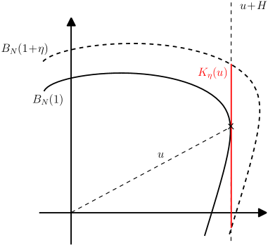
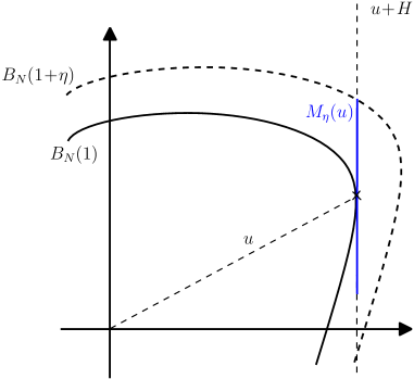
Figure 1: Illustration of the sets $K_{\eta}(u)$ and $M_{\eta}(u)$ (note that $M_{\eta}(u)$ is here strictly included in $K_{\eta}(u)$).

We first prove Proposition 2.

Proof of Proposition 2.

Let $u\in\mathbb{R}^{d}$ such that $N(u)=1$. Let $H$ be a supporting hyperplane of $B_{N}(1)$ at $u$. Let $\eta\geq 0$. We recall the following definitions (see Figure 1 for an illustration):

$$K_{\eta}(u):=\{v\in H\,:\,N(u+v)\leq 1+\eta\}\qquad\mbox{ and }\qquad M_{\eta}(u):=K_{\eta}(u)\cap(-K_{\eta}(u))$$

and

$$h_{u}(\eta):=\eta^{-d}|K_{\eta}(u)|\qquad\mbox{ and }\qquad\bar{h}_{u}(\eta):=\eta^{-d}|M_{\eta}(u)|.$$

Let us prove that $h_{u}$ is a continuous decreasing homeomorphism from $(0,\infty)$ to $(0,\infty)$. The reader can check that the proof can be easily adapted to show that $\bar{h}_{u}$ is also a continuous decreasing homeomorphism from $(0,\infty)$ to $(0,\infty)$.

First notice that $v\in H\mapsto N(u+v)$ is convex. Indeed, for all $v,v^{\prime}\in H$, for all $\lambda\in[0,1]$, we have

$$N(u+\lambda v+(1-\lambda)v^{\prime}) =N(\lambda(u+v)+(1-\lambda)(u+v^{\prime}))$$

$$\leq N(\lambda(u+v))+N((1-\lambda)(u+v^{\prime}))=\lambda N(u+v)+(1-\lambda)N(u+v^{\prime})\,.$$

By convexity, for all $\lambda\in[0,1]$ and $\eta,\eta^{\prime}>0$ we have

$$\lambda K_{\eta}(u)+(1-\lambda)K_{\eta^{\prime}}(u)\subset K_{\lambda\eta+(1-\lambda)\eta^{\prime}}(u)$$

so

$$|K_{\lambda\eta+(1-\lambda)\eta^{\prime}}(u)|^{\frac{1}{d-1}}\geq|\lambda K_{\eta}(u)+(1-\lambda)K_{\eta^{\prime}}(u)|^{\frac{1}{d-1}}.$$

Using Brunn-Minkowski’s inequality, we have

$$|\lambda K_{\eta}(u)+(1-\lambda)K_{\eta^{\prime}}(u)|^{\frac{1}{d-1}}\geq\lambda|K_{\eta}(u)|^{\frac{1}{d-1}}+(1-\lambda)|K_{\eta^{\prime}}(u)|^{\frac{1}{d-1}}\,,$$

so

$$\eta\mapsto|K_{\eta}(u)|^{\frac{1}{d-1}}$$ (9)

is concave and so, in particular, is continuous. This already proves that $h_{u}$ is continuous. Let $v\in H$ and $\eta>0$. For all $\lambda\in[0,1]$, by convexity, we have

$$N(u+\lambda v)\leq\lambda N(u+v)+(1-\lambda)N(u)=\lambda N(u+v)+(1-\lambda)$$

thus

$$N(u+v)-1\leq\eta\implies N(u+\lambda v)-1\leq\lambda\eta\,,$$

and so

$$\lambda K_{\eta}(u)\subset K_{\lambda\eta}(u)\,.$$

This gives that for all $0<\eta_{1}\leq\eta_{2}$,

$$\left(\frac{\eta_{1}}{\eta_{2}}\right)^{d-1}|K_{\eta_{2}}(u)|\leq|K_{\eta_{1}}(u)|$$

so the function $r_{u}(\eta):=\frac{|K_{\eta}(u)|}{\eta^{d-1}}$ is non-increasing. This implies that $h_{u}(\eta)=r_{u}(\eta)/\eta$ is decreasing. Moreover, by triangle inequality, we have, for any $u\in\mathbb{R}^{d}$ such that $N(u)=1$,

$$\{v\in H\,:\,N(v)\leq\eta\}\subset K_{\eta}(u)\subset\{v\in H\,:\,N(v)\leq 2+\eta\}.$$

Using that $N$ is equivalent to the euclidean norm, we get, for some constants $c,c^{\prime}$ depending only on $d$ and $N$,

$$\{v\in H,\|v\|_{2}\leq c\eta\}\subset K_{\eta}(u)\subset\{v\in H,\|v\|_{2}\leq c^{\prime}(2+\eta)\}.$$

Since $H$ is $(d-1)$-dimensional, this gives that, for some $A:=A(d,N)>0$ and $B:=B(d,N)>0$,

$$A\eta^{d-1}\leq|K_{\eta}(u)|\leq B(2+\eta)^{d-1}\,,$$

and so

$$A\eta^{-1}\leq h_{u}(\eta)\leq B\eta^{-d}(2+\eta)^{d-1}.$$

This implies in particular that $h_{u}$ tends to $+\infty$ at 0 and to $0$ at infinity, and for $\eta\in(0,1)$,

$$A\eta^{-1}\leq h_{u}(\eta)\leq B^{\prime}\eta^{-d}.$$

∎

We now state a geometrical lemma that will be useful in what follows.

Lemma 9.

For $u\in\mathbb{R}^{d}$ such that $N(u)=1$ and $H$ a supporting hyperplane of $B_{N}(1)$ at $u$, let denote by $u^{\star}$ the vector normal to $H$ such that $u\cdot u^{\star}=1$. There exist two constants $c,c^{\prime}>0$ depending only on $d$ and $N$ such that, for all $u\in B_{N}(1)$,

$$c\leq\|u^{\star}\|_{2}\leq c^{\prime}.$$

Proof.

Using that $N$ and $||\cdot||_{2}$ are equivalent, there exist $\alpha,\beta>0$ such that

$$B_{\|\cdot\|_{2}}(\alpha)\subset B_{N}(1)\subset B_{\|\cdot\|_{2}}(\beta).$$

So, we get the lower bound on $\|u^{\star}\|_{2}$ noticing that, for $u\in B_{N}(1)$,

$$1=u\cdot u^{\star}\leq\|u\|_{2}\|u^{\star}\|_{2}\leq\beta\|u^{\star}\|_{2}.$$

Moreover, $H$ is a supporting hyperplane of $B_{N}(1)$ at $u$ and $u^{\star}$ is normal to $H$ so $B_{N}(1)$ is included in $\{v\in\mathbb{R}^{d}\,:\,v\cdot u^{\star}\leq u\cdot u^{\star}\}$. Applying this inequality to $\alpha u^{\star}/\|u^{\star}\|_{2}\in B_{\|\cdot\|_{2}}(\alpha)\subset B_{N}(1)$, we get

$$\alpha\|u^{\star}\|_{2}=\alpha\frac{u^{\star}}{\|u^{\star}\|_{2}}\cdot u^{\star}\leq u\cdot u^{\star}=1.$$

Finally, we get

$$\beta^{-1}\leq\|u^{\star}\|_{2}\leq\alpha^{-1}.$$

∎

We introduce now a function $I$ defined by an integral and check that this function is of the same order as the function $h_{u}$ whose inverse $g_{u}$ appears in the statement of Theorem 3. We recall that for $\eta\geq 0$, $h_{u}(\eta)$ is defined by

$$h_{u}(\eta)=\eta^{-d}|K_{\eta}(u)|\,.$$

Lemma 10.

For $u\in\mathbb{R}^{d}$ such that $N(u)=1$ and $H$ a supporting hyperplane of $B_{N}(1)$ at $u$, let denote by $u^{\star}$ the vector normal to $H$ such that $u\cdot u^{\star}=1$ and define, for $\eta>0$,

$$I^{+}(\eta)=\int_{\mathbb{R}^{d}\cap\{x:x\cdot u^{\star}>0\}}\exp(-(N(x)-(1-\eta)x\cdot u^{\star}))dx.$$

Then there exists two constant $c_{1},c_{2}$ depending only on $N$ and $d$ such that, for $\eta>0$, we have

$$c_{1}h_{u}(\eta)\leq I^{+}(\eta)\leq c_{2}h_{u}(\eta).$$ (10)

Moreover, define also, for $\eta>0$,

$$I(\eta)=\int_{\mathbb{R}^{d}}\exp(-(N(x)-(1-\eta)x\cdot u^{\star}))dx\,,$$

then for $\eta$ small enough, we have

$$c_{1}h_{u}(\eta)\leq I(\eta)\leq 2c_{2}h_{u}(\eta).$$ (11)

Proof.

Let $\|\cdot\|_{2}$ be the Euclidean norm. Let $\overline{\psi}:=\overline{\psi}_{\eta}:H\rightarrow H$ be an affine transformation with positive determinant such that

$$N(u+\overline{\psi}(t))\leq 1+\eta\textrm{ for all }t\in H\textrm{ such that }\|t\|_{2}\leq 1$$ (12)

and

$$N(u+\overline{\psi}(t))\geq 1+\eta\textrm{ for all }t\in H\textrm{ such that }\|t\|_{2}\geq d-1.$$ (13)

Let us prove that such an application $\overline{\psi}$ exists. The set

$$K_{\eta}(u)=\{v\in H\,:\,N(u+v)\leq 1+\eta\}$$

is compact, convex, with non-empty interior. Thus, by John-Loewner Theorem (see for instance Theorem III in [14]), there exists a centered ellipsoïde $J$ of $H$ and a $c\in H$ such that

$$c+J\subset K_{\eta}(u)\subset c+(d-1)J.$$

Let $B_{H}(r):=B_{\|\cdot\|_{2},H}(r)$ be the ball of $H$ of radius $r$ for the Euclidean norm $\|\cdot\|_{2}$. Let $\psi:H\mapsto H$ be the linear function with positive determinant such that $\psi(B_{H}(1))=J$ and $\overline{\psi}:=c+\psi$. Then, we have

$$\overline{\psi}(B_{H}(1))=c+J\subset K_{\eta}\subset c+(d-1)J=\overline{\psi}(B_{H}(d-1))$$

which shows that (12) and (13) hold. Moreover, we can find bounds on the determinant of $\psi$. Indeed, we have

$$\det(\psi)=\frac{|\psi(B_{H}(1))|}{|B_{H}(1)|}=\frac{|\psi(B_{H}(1))|}{V_{d-1}}$$

where $V_{d-1}$ is the volume of the unit euclidean ball of $\mathbb{R}^{d-1}$. Using that

$$|\psi(B_{H}(1))|\leq|K_{\eta}(u)|\leq|\psi(B_{H}(d-1))|$$

we get

$$V_{d-1}\det(\psi)\leq|K_{\eta}(u)|\leq(d-1)^{d-1}V_{d-1}\det(\psi)$$ (14)

Recall now that

$$I^{+}(\eta)=\int_{\mathbb{R}^{d}\cap\{x:x\cdot u^{\star}>0\}}\exp(-(N(x)-(1-\eta)x\cdot u^{\star}))dx\,.$$

By the change of variable $x=\lambda u+v$ with $\lambda=x\cdot u^{\star}$ and $v\in H$, we have

$$I^{+}(\eta) =\frac{1}{\|u^{\star}\|_{2}}\int_{0}^{\infty}\int_{H}\exp(-(N(\lambda u+v)-(1-\eta)\lambda))dv\,d\lambda$$

$$=\frac{1}{\|u^{\star}\|_{2}}\int_{0}^{\infty}\int_{H}\lambda^{d-1}\exp\left(-\eta\lambda-\eta\lambda\frac{N(u+w)-1}{\eta}\right)dw\,d\lambda\,.$$

Let $x=\lambda\eta$ and $w=\overline{\psi}(t)$. Then

$$I^{+}(\eta)=\frac{1}{\|u^{\star}\|_{2}}\eta^{-d}\det(\psi)G(\eta)$$

with

$$G(\eta)=\int_{0}^{\infty}\int_{H}x^{d-1}\exp\left(-x-x\frac{N(u+\overline{\psi}(t))-1}{\eta}\right)dt\,dx\,.$$

Let us prove that there exists two constants $c,c^{\prime}>0$ (depending only on $N$ and $d$) such that $c\leq G(\eta)\leq c^{\prime}$ for $\eta>0$. Let define

$$g_{\eta}(t):=\frac{N(u+\overline{\psi}(t))-1}{\eta}\,.$$

First recall that if $t\in B_{H}(1)$, then $g_{\eta}(t)\leq 1$. Thus

$$G(\eta)\geq\int_{0}^{\infty}\int_{B_{H}(1)}x^{d-1}\exp(-2x)dt\,dx=V_{d-1}\int_{0}^{\infty}x^{d-1}\exp(-2x)dx=\frac{V_{d-1}d!}{2^{d}}:=c\,.$$

On the other side, if $\|t\|_{2}\geq d$ then $g_{\eta}(t)\geq 1$. Let $t_{0}=\overline{\psi}^{-1}(0)$. Note that $g_{\eta}(t_{0})=0$ and so $\|t_{0}\|_{2}\leq d$. Using the convexity of $g_{\eta}$, we get that for $\|t\|_{2}\geq d$,

$$g_{\eta}(t)\geq\frac{\|t-t_{0}\|_{2}}{d+\|t_{0}\|_{2}}\geq\frac{\|t\|_{2}}{2d}-\frac{1}{2}\,.$$

Since $g_{\eta}$ is non-negative on $H$, this lower bound holds in fact on $H$. This yields

$$G(\eta) \leq\int_{0}^{\infty}\int_{H}x^{d-1}\exp\left(-x-x\left(\frac{\|t\|_{2}}{2d}-\frac{1}{2}\right)\right)dt\,dx$$

$$\leq\int_{0}^{\infty}\int_{\mathbb{R}^{d-1}}x^{d-1}\exp\left(-\frac{x}{2}-\frac{\|xt\|_{2}}{2d}\right)dt\,dx$$

$$\leq\int_{0}^{\infty}\exp(-\frac{x}{2})dx\int_{\mathbb{R}^{d-1}}\exp\left(-\frac{\|v\|_{2}}{2d}\right)dv:=c^{\prime}\,<\,\infty\,.$$

Hence we get, using (14), that for $\eta>0$

$$\frac{c}{\|u^{\star}\|_{2}}((d-1)^{d-1}V_{d-1})^{-1}|K_{\eta}(u)|\leq\eta^{d}I^{+}(\eta)\leq\frac{c^{\prime}}{\|u^{\star}\|_{2}}(V_{d-1})^{-1}|K_{\eta}(u)|\,.$$

We conclude the study of $I^{+}(\eta)$ using Lemma 9 which bounds $\|u^{\star}\|_{2}$ uniformly in $u\in B_{N}(1)$. We now study $I(\eta)$ defined by

$$I(\eta)=\int_{\mathbb{R}^{d}}\exp(-(N(x)-(1-\eta)x\cdot u^{\star}))dx.$$

We have $I(\eta)=I^{+}(\eta)+I^{-}(\eta)$ where

$$I^{-}(\eta)=\int_{\mathbb{R}^{d}\cap\{x:x\cdot u^{\star}<0\}}\exp(-(N(x)-(1-\eta)x\cdot u^{\star}))dx.$$

Note that for $\eta\in[0,1]$, $0\leq I^{-}(\eta)\leq\int_{\mathbb{R}^{d}}\exp(-N(x))dx<\infty$ so $I^{-}$ is bounded around $0$. On the contrary, since $I^{+}(\eta)$ is of the same order as $h_{u}(\eta):=K_{\eta}(u)\eta^{-d}$, Proposition 2 implies that $I^{+}$ tends to infinity at $0$. So we get that $I(\eta)\sim I^{+}(\eta)$ for $\eta$ going to $0$ and so for $\eta$ small enough, we have

$$c_{1}h_{u}(\eta)\leq I(\eta)\leq 2c_{2}h_{u}(\eta)$$

as desired. ∎

4 Proof of the lower bound on $1-\mu_{\varepsilon}(u)$

This section is devoted to the proof of a lower bound on $1-\mu_{\varepsilon}(u)$, i.e., the proof of Proposition 11 - and incidentally, as a corollary, we get a lower bound on $\sharp\gamma_{\varepsilon}(su)$ for large $s$ too, see Corollary 12 below. To do so, it is enough to exhibit a path from $0$ to $su$ (for a given direction $u$ and $s$ large enough) whose $N$-length is not too high, but that gather enough rewards. This is done in Proposition 11 through a greedy algorithm. This algorithm adds recursively to the path $\pi=(0,x_{1}\cdots,x_{n-1})$ the closest point $x_{n}$ of the Poisson point process $\Xi$ (in a certain sense) which is located in a cone with origin $x_{n-1}$ and oriented in the direction $u$. This cone condition gives us a good upper bound on the $N$-length of the path we construct. However, we have to be careful in our procedure to be sure that the path $\pi$ does not go too far away from the prescribed direction $u$. We thus take care to compensate any gap previously created between the direction of $x_{n-1}$ and the prescribed direction $u$ by choosing wisely the direction of the next point $x_{n}$ the path collects. At this stage, we need to deal with some symmetries, this is the reason why it is the set $M_{\eta}(u)$, which is a symmetrized version of $K_{\eta}(u)$, that arises in the proof.

Fix a direction $u\in\mathbb{R}^{d}$ with $N(u)=1$, $H$ a supporting hyperplane of $B_{N}(1)$ at $u$ and recall that

$$M_{\eta}(u):=\{v\in H\,:\,N(u+v)\leq 1+\eta\mbox{ and }N(u-v)\leq 1+\eta\}\qquad\mbox{ and }\qquad\bar{h}_{u}(\eta):=\eta^{-d}|M_{\eta}(u)|\,.$$

Proposition 2 states that $\eta\mapsto\bar{h}_{u}(\eta)$ is a continuous decreasing homeomorphism from $(0,\infty)$ to $(0,\infty)$ so we can define its inverse function $\bar{g}_{u}$ which is also a continuous decreasing homeomorphism from $(0,\infty)$ to $(0,\infty)$. To prove the lower bound on $1-\mu_{\varepsilon}(u)$ given in (i) of Theorem 3, we prove in fact the following proposition.

Proposition 11.

There exists a constant $c>0$ (depending only on $d,N$) such that, for all direction $u\in\mathbb{R}^{d}$ with $N(u)=1$, for all $\eta\in(0,1)$, we have

$$\mu_{\varepsilon}(u)\leq 1+\eta-c\varepsilon^{1/d}|M_{\eta}(u)|^{1/d}.$$

In particular, with $C_{1}:=\left(\frac{2}{c}\right)^{d}$, we have that for $\varepsilon$ small enough,

$$\mu_{\varepsilon}(u)\leq 1-\bar{g}_{u}\left(C_{1}\varepsilon^{-1}\right)\,.$$

Proof.

To prove this proposition, we construct, using a greedy algorithm, a path $\pi_{s}$ from $0$ to $su$ with length close to $s(1+\eta)$ but going through a number of points of $\Xi$ larger than $c|M_{\eta}(u)|^{1/d}s$ (see Figure 2).

We first introduce some notation. For $s\geq 0$, let

$$C_{\eta}(s) :=\{x=\lambda u+v\,:\,0\leq\lambda\leq s\,,\,v\in H\,,\,N(\lambda u+v)\leq\lambda(1+\eta),N(\lambda u-v)\leq\lambda(1+\eta)\}\,.$$

Hence, $C_{\eta}(s)$ is a cone with axis $u$ and of basis $M_{\eta}$ (basis not necessarily orthogonal to its axis). Thus, if $u^{\star}$ denotes the vector orthogonal to $H$ such that $u\cdot u^{\star}=1$, we have

$$|C_{\eta}(s)|=\frac{1}{d\|u^{\star}\|_{2}}|M_{\eta}(u)|s^{d}.$$

In the algorithm, we construct a path $(0,x_{1},\dots,x_{n},su)$ from $0$ to $su$ such that $x_{i+1}$ is the first point of $\Xi$ in the cone $x_{i}+C_{\eta}(\infty)$. By construction, we prove that the length of such path cannot be much larger than $(1+\eta)s$ and its number of points is at least of order $|M_{\eta}(u)|^{1/d}s$. Optimizing on $\eta$ yields then Proposition 11.

Recall that $\Xi$ denotes the points of a Poisson point process with intensity $|\cdot|$ on $\mathbb{R}^{d}$. By induction we define a sequence $(X_{n})_{n\geq 0}$ in $\mathbb{R}^{d}$ with $X_{0}=0$ and if

$$\lambda_{n+1}:=\inf\{s>0\,:\,(X_{n}+C_{\eta}(s))\cap\Xi\neq\emptyset\}\,,$$

we set $X_{n+1}=X_{n}+\lambda_{n+1}u+W_{n+1}$ with $W_{n+1}\in H$ and such that $\{X_{n+1}\}=(X_{n}+C_{\eta}(\lambda_{n+1}))\cap\Xi$. We define $S_{n}=\sum_{i=1}^{n}\lambda_{i}$ and $V_{n}=\sum_{i=1}^{n}W_{i}$. By the proprieties of Poisson point processes, $(\lambda_{i})_{i\geq 1}$ and $(W_{i})_{i\geq 1}$ are i.i.d. random variables and since $M_{\eta}(u)$ is a symmetric set, $W_{1}$ has also a symmetric distribution and so $V_{n}$ is a symmetric random walk.

Let us now define, for $s>0$,

$$Z(s):=\sup\{n\geq 0\,:\,S_{n}\leq s\}$$

and consider the path $\pi_{s}=(0,X_{1},\dots,X_{Z(s)},su)$ (see Figure 2 for an illustration of the greedy algorithm). Let us find an upper bound of $T_{\varepsilon}(\pi_{s})$ by finding an upper bound of its length and a lower bound of $Z(s)$, its number of points.

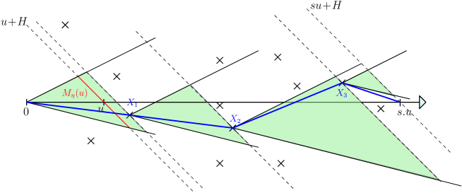
Figure 2: Illustration of the greedy algorithm. The path constructed is drawn in blue. At each step, the path goes through the first point of $\Xi$ in the green cone in front of it.

The sequence $(\lambda_{i})_{i\geq 1}$ is i.i.d. and we have

$$\mathbb{P}(\lambda_{1}\geq t) =\exp\left(-\frac{1}{d\|u^{\star}\|_{2}}|M_{\eta}(u)|t^{d}\right)$$

so that

$$\mathbb{E}(\lambda_{1})=\left(\frac{|M_{\eta}(u)|}{d\|u^{\star}\|_{2}}\right)^{-1/d}\int_{0}^{\infty}\exp(-v^{d})dv:=\frac{|M_{\eta}|^{-1/d}}{2c_{u}}$$

where

$$2c_{u}:=\left(\frac{1}{d\|u^{\star}\|_{2}}\right)^{1/d}\left(\int_{0}^{\infty}\exp(-v^{d})dv\right)^{-1}.$$

Since $S_{n}=\sum_{i=1}^{n}\lambda_{i}$, a standard renewal theorem yields that, for $s$ large enough, we have

$$c_{u}|M_{\eta}(u)|^{1/d}s\leq Z(s)\leq 3c_{u}|M_{\eta}(u)|^{1/d}s\,.$$ (15)

This gives a lower bound for the number of points of $\pi_{s}$. It remains now to find an upper bound for the length of $\pi_{s}$. Note first that if we consider the path $\pi^{\prime}_{s}=(0,X_{1},\dots,X_{Z(s)})$, we have by construction

$$N(X_{i+1}-X_{i})\leq(1+\eta)\lambda_{i+1}$$

so

$$N(\pi^{\prime}_{s})\leq(1+\eta)S_{Z(s)}\,.$$

Thus

$$N(\pi_{s})\leq(1+\eta)S_{Z(s)}+N(su-(S_{Z(s)}u+V_{Z(s)}))\leq(1+\eta)S_{Z(s)}+s-S_{Z(s)}+N(V_{Z(s)})\leq(1+\eta)s+N(V_{Z(s)})\,.$$

Let us now prove that $N(V_{Z(s)})/s$ tends a.s. to $0$. The process $(V_{k})_{k\geq 0}$ is a symmetric random walk and by construction, we have

$$N(\lambda_{1}u+V_{1})\leq\lambda_{1}(1+\eta)$$

which yields

$$N(V_{1})\leq\lambda_{1}(1+\eta)+N(\lambda_{1}u)\leq 3\lambda_{1}$$

for $\eta\in(0,1)$. This implies that $\mathbb{E}(N(V_{1}))$ is finite. Using that for $s$ large enough $Z(s)\leq 3c_{u}|M_{n}|^{1/d}s$ a.s., the law of large number implies that

$$\lim_{n\to\infty}\frac{N(V_{Z(s)})}{s}=0\quad\mbox{a.s.}$$

Hence, for all $\eta\in(0,1)$, we have, for $s$ large enough,

$$T_{\varepsilon}(0,su)\leq T_{\varepsilon}(\pi_{s})\leq s\left(1+\eta+\frac{N(V_{Z(s)})}{s}-\varepsilon^{1/d}c_{u}|M_{\eta}(u)|^{1/d}\right)\,.$$

We deduce

$$\mu_{\varepsilon}(u)=\lim_{s\rightarrow\infty}\frac{T_{\varepsilon}(0,su)}{s}\leq 1+\eta-\varepsilon^{1/d}c_{u}|M_{\eta}(u)|^{1/d}=1-\eta\left(c_{u}\left(\varepsilon\bar{h}_{u}(\eta)\right)^{1/d}-1\right)\,.$$

Let define $c_{1}:=\inf\{c_{u},u\in B_{N}(1)\}$ and note, in view of Lemma 9, that $c_{1}>0$. We get, for all $u\in B_{N}(1)$,

$$\mu_{\varepsilon}(u)\leq 1-\eta\left(c_{1}\left(\varepsilon\bar{h}_{u}(\eta)\right)^{1/d}-1\right)\,.$$

This proves the first part of Proposition 11. Taking

$$\eta=\bar{g}_{u}\left(\left(\frac{2}{c_{1}}\right)^{d}\varepsilon^{-1}\right)\,,$$

(notice that $\eta<1$ for $\varepsilon$ small enough), we obtain that $c_{1}\left(\varepsilon\bar{h}_{u}(\eta)\right)^{1/d}=2$, thus

$$\mu_{\varepsilon}(u)\leq 1-\eta\,.$$

∎

Let us note that this implies a lower bound for the number of points taken by the geodesic, that we state in the following Corollary.

Corollary 12.

Let $C_{1}=C_{1}(d,N)$ be the constant given by Proposition 11. For $\varepsilon$ small enough, we have, for any $\delta>0$, a.s. for large $s$,

$$\varepsilon^{1/d}\sharp\gamma_{\varepsilon}(su)\geq(1-\delta)\bar{g}_{u}(C_{1}\varepsilon^{-1})s\,,$$ (16)

where $\gamma_{\varepsilon}(su)$ denotes any geodesic from $0$ to $su$ for the time $T_{\varepsilon}(0,su)$.

Proof.

Indeed, if $\gamma_{\varepsilon}(su)$ denotes a geodesic from $0$ to $su$, we have

$$\varepsilon^{1/d}\sharp\gamma_{\varepsilon}(su)=N(\gamma_{\varepsilon}(su))-T_{\varepsilon}(0,su)\geq s\left(1-\frac{T_{\varepsilon}(0,su)}{s}\right)\,.$$

Using that $1-\frac{T_{\varepsilon}(0,su)}{s}$ converges to $1-\mu_{\varepsilon}(u)$ and Proposition 11, we get that for any $\varepsilon$ small enough, for any $\delta>0$, a.s. for $s$ large enough,

$$\varepsilon^{1/d}\sharp\gamma_{\varepsilon}(su)\geq(1-\delta)\bar{g}_{u}(C_{1}\varepsilon^{-1})s\,.$$

∎

5 Proof of the upper bound on $1-\mu_{\varepsilon}(u)$

We want now to find the lower bound for $\mu_{\varepsilon}(u)$ of Theorem 3. In the course of the proof, we will also prove the upper bounds on the length and the number of rewards of the geodesic stated in Point (ii) of the theorem. The idea of the proof is the following. For any geodesic $\gamma_{\varepsilon}(su)$ from 0 to $su$, we have

$$N(\gamma_{\varepsilon}(su))=T_{\varepsilon}(0,su)+\varepsilon^{1/d}\sharp\gamma_{\varepsilon}(su)\leq s+\varepsilon^{1/d}\sharp\gamma_{\varepsilon}(su).$$ (17)

Any upper bound on $\sharp\gamma_{\varepsilon}(su)$ thus provides an upper bound on $N(\gamma_{\varepsilon}(su))$. In the next proposition, we prove that, for any $\eta>0$ small enough, for any $s$ large enough and any path $\pi$ from 0 to $su$, we have

$$N(\pi)\leq(1+\eta)s\;\Longrightarrow\;\sharp\pi\leq c|K_{\eta}(u)|^{1/d}s.$$ (18)

In particular, any good upper bound on $N(\gamma_{\varepsilon}(su))$ provides in turn an upper bound on $\sharp\gamma_{\varepsilon}(su)$. We then prove the following crude inequality (see (23)): for some constant $c$, almost surely, for any path $\pi$ from 0 to a faraway point,

$$\sharp\pi\leq cN(\pi).$$ (19)

Plugging (19) in (17) gives a first upper bound on $N(\gamma_{\varepsilon}(su))$ (see (22)). Using repeatedly and alternately (17) and (18), we then get, after a finite number of steps, the upper bounds on $N(\gamma_{\varepsilon}(su))$ and $\sharp\gamma_{\varepsilon}(su)$ given in Theorem 3. From the upper bound on $\sharp\gamma_{\varepsilon}(su)$ we deduce straightforwardly a lower bound on $\mu_{\varepsilon}(u)$. We conclude this section by noticing that, at least under some added hypothesis, we can recover a lower bound on $N(\gamma_{\varepsilon}(su))$ (see Proposition 15) by a final last use of Proposition 13 and the lower bound on $\sharp\gamma_{\varepsilon}(su)$ proved in Section 4 (see Corollary 12).

We start by proving the following proposition, that states that a path from $0$ to $su$ with small $N$-length cannot collect too much rewards.

Proposition 13.

Let consider the event

$$\mathcal{E}(\eta,s,u,c):=\{\exists\pi\in\Pi(0,su),N(\pi)\leq(1+\eta)s,\sharp\pi\geq c|K_{\eta}(u)|^{1/d}s\}.$$

Then there exists some $c,c^{\prime}>0$ depending only on $d$ and $N$ such that for any $u\in B_{N}(1)$ and any hyperplane $H$ which is a supporting hyperplane of $B_{N}(1)$ at $u$, there exists $\bar{\eta}>0$ (depending only on $d,u,H$) such that, for $\eta<\bar{\eta}$, for all $s>0$, we have

$$\mathbb{P}[\mathcal{E}(\eta,s,u,c)]\leq 2\exp[-sc^{\prime}|K_{\eta}(u)|^{1/d}].$$ (20)

In particular, for all $\eta\in(0,\bar{\eta})$ there exists a.s. $s_{\eta}$ such that, for $s\geq s_{\eta}$, every path $\pi\in\Pi(0,su)$ such that $N(\pi)\leq(1+\eta)s$ satisfies $\sharp\pi\leq c|K_{\eta}(u)|^{1/d}s$.

To prove this proposition, we will need the following lemma which roughly states the same thing except that we consider now a path from the origin $0$ to the hyperplane $su+H$. We denote by $\Pi(0,su+H)$ the set of all polygonal paths $\pi\in\Pi(0,y)$ for some $y\in su+H$.

Lemma 14.

For $A>0$ and $H$ a supporting plane of $B_{N}(1)$ at $u$, define

$$\mathcal{E}(\eta,s,u,A,H):=\{\exists\pi\in\Pi(0,su+H),\forall x\in\pi,x\cdot u^{\star}\leq s,N(\pi)\leq(1+\eta)s,\sharp\pi\geq As\}.$$

Then, for all $s>0$ and $\eta>0$,

$$\mathbb{P}[\mathcal{E}(\eta,s,u,A,H)]\leq\exp[-s(A\log 2-2^{1+1/d}I(\eta)^{1/d}\eta)]\,.$$

We first explain how Lemma 14 implies the proposition.

Proof of Proposition 13 using Lemma 14.

A path $\pi\in\Pi(0,su)$ can be decomposed into two paths $\pi_{1}$ and $\pi_{2}$ where $\pi_{1}$ is the restriction of the path $\pi$ until it intersects the hyperplane $su+H$ and $\pi_{2}$ is the intersection of the path $\pi$ afterwards. Note that $N(\pi)=N(\pi_{1})+N(\pi_{2})$ and moreover $N(\pi_{1})\geq s$. If $\pi$ satisfies the property appearing in the definition of the event $\mathcal{E}(\eta,s,u,c)$, we thus get $N(\pi_{2})\leq\eta s$ and moreover we have either $\sharp\pi_{1}\geq c|K_{\eta}(u)|^{1/d}s/2$ or $\sharp\pi_{2}\geq c|K_{\eta}(u)|^{1/d}s/2$. Hence, if we define

$$\mathcal{F}(\eta,s,u,c):=\{\exists\pi\in\Pi(su,\star),N(\pi)\leq\eta s,\sharp\pi\geq\frac{c}{2}|K_{\eta}(u)|^{1/d}s\}\,,$$

we get

$$\mathcal{E}(\eta,s,u,c)\subset\mathcal{E}\left(\eta,s,u,\frac{c}{2}|K_{\eta}(u)|^{1/d},H\right)\cup\mathcal{F}(\eta,s,u,c)\,.$$

Using (11) in Lemma 10, we see that we can choose $c$ such that for $\eta$ small enough we have

$$\frac{c|K_{\eta}(u)|^{1/d}}{2}\log 2\geq\eta 5I(\eta)^{1/d}$$

so that

$$\frac{c|K_{\eta}(u)|^{1/d}}{2}\log 2-2^{1+1/d}I(\eta)^{1/d}\eta\geq I(\eta)^{1/d}\eta(5-4)=I(\eta)^{1/d}\eta.$$

Thus by Lemma 14 we get

$$\mathbb{P}\left[\mathcal{E}\left(\eta,s,u,\frac{c}{2}|K_{\eta}(u)|^{1/d},H\right)\right]\leq\exp[-sI(\eta)^{1/d}\eta)]\leq\exp[-sc_{1}|K_{\eta}(u)|^{1/d}]$$

for some constant $c_{1}$. Moreover, let $q=\frac{c}{2}|K_{\eta}(u)|^{1/d}s$, then for any $\beta>0$,

$$\mathbb{P}[\mathcal{F}(\eta,s,u,c)] = \mathbb{P}[\exists\pi\in\Pi(0,\star),N(\pi)\leq\eta s,\sharp\pi\geq q]$$

$$\leq \mathbb{P}[\exists(x_{1},\ldots,x_{q})\in\Xi,\;\sum_{i=1}^{q}N(x_{i}-x_{i-1})\leq\eta s]$$

$$= \exp(\beta\eta s)\left(\int\exp(-\beta N(x))dx\right)^{q}$$

$$= \exp(\beta\eta s)\left(\frac{1}{\beta^{d}}\int\exp(-N(x))dx\right)^{q}\,.$$

Chose $\beta_{0}:=\beta_{0}(d)$ such that the bracket above is equal to $1/2$. Then

$$\mathbb{P}[\mathcal{F}(\eta,s,u,c)] \leq \exp(\beta_{0}\eta s-q\log 2)$$

$$= \exp\left(-\eta s\left(\frac{c}{2}h_{u}(\eta)^{1/d}\log 2-\beta_{0}\right)\right),$$

where $h_{u}(\eta)=\eta^{-d}|K_{\eta}(u)|$. By Proposition 2, $h_{u}(\eta)$ tends to infinity as $\eta$ tends to 0, we choose $\bar{\eta}:=\bar{\eta}(d,u,H)$ such that $\beta_{0}\leq\frac{c}{4}h_{u}(\eta)^{1/d}(2\log 2-1)$ for $\eta\leq\bar{\eta}$. This yields

$$\mathbb{P}[\mathcal{F}(\eta,s,u,c)]\leq\exp\left[-s\frac{c}{4}|K_{\eta}(u)|^{1/d})\right].$$

This implies that (20) holds with $c^{\prime}=\min(c_{1},c/4)$. Moreover, if we set $\lambda_{n}=n/(c|K_{\eta}(u)|^{1/d})$, we get

$$\sum_{n=1}^{\infty}\mathbb{P}[\mathcal{E}(\eta,\lambda_{n},u,c)]\leq 2\sum_{n=1}^{\infty}\exp\left[-\frac{c^{\prime}}{c}n\right]\,.$$

Thus, Borel-Cantelli Lemma yields that for $n$ large enough, every path $\pi\in\Pi(0,\lambda_{n}u)$ such that $N(\pi)\leq(1+\eta)\lambda_{n}$ satisfies $\sharp\pi<c|K_{\eta}(u)|^{1/d}\lambda_{n}=n$. Then for $s\in[\lambda_{n},\lambda_{n+1}[$, if $\pi$ is a path from $0$ to $su$ such that $N(\pi)\leq(1+\eta)s$, adding to $\pi$ a straight line colinear to $u$ yields a path from $0$ to $\lambda_{n+1}u$ such that $N(\pi)\leq(1+\eta)\lambda_{n+1}$. Thus we deduce that $\sharp\pi<n+1$. Since $\lfloor c|K_{\eta}(u)|^{1/d}s\rfloor=n$, this implies in fact that $\sharp\pi\leq c|K_{\eta}(u)|^{1/d}s$. ∎

We now prove Lemma 14.

Proof of Lemma 14.

Let $q=\lceil As\rceil$. Let $\pi=(0,x_{1},\ldots,x_{q},x_{q+1})\in\Pi(0,su+H)$ where $x_{1},\ldots,x_{q}$ are points of the $\Xi$ and $x_{q+1}-x_{q}$ is colinear to $u$. Set $x_{0}=0$. Thus

$$N(\pi)=\sum_{i=1}^{q+1}N(x_{i}-x_{i-1})=\sum_{i=1}^{q}N(x_{i}-x_{i-1})+|s-x_{q}\cdot u^{\star}|=\sum_{i=1}^{q}N(x_{i}-x_{i-1})+s-x_{q}\cdot u^{\star}\,.$$

Thus

$$N(\pi)\leq(1+\eta)s\Leftrightarrow\sum_{i=1}^{q}N(x_{i}-x_{i-1})\leq\eta s+x_{q}\cdot u^{\star}.$$

We get for any $\alpha,\beta>0$,

$$\mathbb{P}[\mathcal{E}(\eta,s,u,A,H)] = \mathbb{P}(\exists x_{1},\ldots,x_{q}\in\Xi,x_{q}\cdot u^{\star}\leq s,\sum_{i=1}^{q}N(x_{i}-x_{i-1})\leq\eta s+x_{q}\cdot u^{\star})$$

$$\leq \int_{(\mathbb{R}^{d})^{q}}\exp\left(\beta(s-x_{q}\cdot u^{\star})+\alpha\left(\eta s-\sum_{i=1}^{q}N(x_{i}-x_{i-1})+x_{q}\cdot u^{\star}\right)\right)dx_{1}\ldots dx_{q}\,.$$

Taking $\beta=\alpha\eta$, we get

$$\mathbb{P} [\mathcal{E}(\eta,s,u,A,H)]$$

$$\leq\exp(2\alpha\eta s)\int_{(\mathbb{R}^{d})^{q}}\exp\left(-\alpha\left(\sum_{i=1}^{q}N(x_{i}-x_{i-1})-(1-\eta)\sum_{i=1}^{q}(x_{i}-x_{i-1})\cdot u^{\star}\right)\right)dx_{1}\ldots dx_{q}$$

$$=\exp(2\alpha\eta s)\left(\int_{\mathbb{R}^{d}}\exp\left(-\alpha(N(x)-(1-\eta)x\cdot u^{\star})\right)dx\right)^{q}$$

$$=\exp(2\alpha\eta s)\left(\frac{I(\eta)}{\alpha^{d}}\right)^{q}.$$

We conclude taking $\alpha$ such that $\alpha^{d}=2I(\eta)$.

∎

We can now prove the upper bound on the number of points and the length of a geodesic given in (ii) of Theorem 3, i.e., we can prove that there exists a constant $C_{2}$ (depending only on $d$ and $N$) such that if $\gamma_{\varepsilon}(su)$ is a geodesic from $0$ to $su$, then, for $\varepsilon$ small enough, we have for any $\delta>0$, a.s., for $s$ large enough

$$N(\gamma_{\varepsilon}(su))\leq s(1+(1+\delta)g_{u}(C_{2}\varepsilon^{-1}))\textrm{ and }\sharp\gamma_{\varepsilon}(su)\leq(1+\delta)g_{u}(C_{2}\varepsilon^{-1})\varepsilon^{-1/d}s.$$ (21)

Proof of (21).

We begin by proving that there exists some $C>0$ such that, for $\varepsilon$ small enough, we have a.s. for $s$ large enough

$$N(\gamma_{\varepsilon}(su))\leq s[1+C\varepsilon^{1/d}]\,.$$ (22)

We use tools that come from the study of the greedy paths and greedy lattice animals. Let

$$G(s):=\sup\left\{\frac{\sharp\pi}{N(\pi)}\,:\,\pi\in\Pi(0,\star)\,,\,\pi\not\subset B_{N}(s)\right\}\leq\sup\left\{\frac{\sharp\pi}{N(\pi)}\,:\,\pi\in\Pi(0,\star)\right\}:=G\,.$$

Let $G(\infty)$ be the increasing limit of $G(s)$. We have the follonwing properties : $G(\infty)\leq G$, $G(\infty)$ is constant a.s. and

$$G(\infty)=\mathbb{E}[G(\infty)]\leq\mathbb{E}[G]\leq c\int_{0}^{\infty}\delta_{1}([r,+\infty[)^{1/d}dr:=C/4\,.$$

This is a consequence of $(11)$ and Lemma 2.1 in [9] (which is the analog in a continuous setting of a result by Martin [19] in a discrete setting), and these results have already been useful to study continuous first-passage percolation (see [10] Theorem 3.1 or [11] Theorem 13 and Corollary 14). Thus, a.s. for large enough $s$, for all $\pi\in\Pi(0,\star)$ such that $\pi\not\subset B_{N}(s/2)$ we have

$$\sharp\pi\leq(C/2)N(\pi)\,.$$ (23)

In particular, this holds for $\gamma_{\varepsilon}(su)$, a geodesic from $0$ to $su$. Using that $T(\gamma_{\varepsilon}(su))\leq s$, we get

$$s\geq T(\gamma_{\varepsilon}(su))=N(\gamma_{\varepsilon}(su))\left[1-\varepsilon^{1/d}\frac{\sharp\gamma_{\varepsilon}(su)}{N(\gamma_{\varepsilon}(su))}\right]\geq N(\gamma_{\varepsilon}(su))[1-C\varepsilon^{1/d}/2]$$

which gives $N(\gamma_{\varepsilon}(su))\leq s[1-C\varepsilon^{1/d}/2]^{-1}\leq s[1+C\varepsilon^{1/d}]$ for $\varepsilon$ small enough.

Let now consider $c>0$ such that the conclusion of Proposition 13 holds, i.e., for any $u\in B_{N}(1)$, for $\eta$ small enough we have a.s. that for $s$ large enough, any path $\pi:0\mapsto su$ such that $N(\pi)\leq(1+\eta)s$ go trough less than $c|K_{\eta}(u)|^{1/d}$ points of $\Xi$. Let now define the sequence $(\eta_{n})_{n\geq 0}$ by

$$\eta_{0}=C\varepsilon^{1/d}\mbox{ and }\eta_{n+1}=c|K_{\eta_{n}}(u)|^{1/d}\varepsilon^{1/d}.$$

The function $\eta\mapsto|K_{\eta}(u)|$ is continuous and increases with $\eta$ so the sequence $(\eta_{n})$ is monotonic. Assume that $\varepsilon$ is small enough such that $C\varepsilon^{1/d}\leq 1$ and $c|K_{1}(u)|^{1/d}\varepsilon^{1/d}\leq 1$. We get then by induction that the the sequence $(\eta_{n})$ remains in $[0,1]$ so it converges to a solution of the equation

$$\eta=c|K_{\eta}(u)|^{1/d}\varepsilon^{1/d}\,,$$

i.e, either to $0$ or to $\eta_{\infty}:=g_{u}((c^{d}\varepsilon)^{-1})$. Note that in both cases, if we fix some $\delta>0$, we have, for $n$ large enough, $\eta_{n}\leq(1+\delta)\eta_{\infty}$.

Assume moreover that $\varepsilon$ is small enough such that Proposition 13 holds for $\eta_{0}$, i.e., $\eta_{0}\leq\bar{\eta}$. Let us prove by induction on $n$ that for all $n\geq 1$, there exists a.s. (a random) $s_{n}$ such that, for $s>s_{n}$, $\sharp\gamma_{\varepsilon}(su)\leq\eta_{n}\varepsilon^{-1/d}s$. We have seen that for $s$ large enough, $N(\gamma_{\varepsilon}(su))\leq s[1+\eta_{0}]$. Using Proposition 13, we get that for $s$ large enough $\sharp\gamma_{\varepsilon}(su)\leq c|K_{\eta_{0}}(u)|^{1/d}s=\eta_{1}\varepsilon^{-1/d}s$. Note that if the sequence $(\eta_{n})$ is non-decreasing, this directly implies that $\sharp\gamma_{\varepsilon}(su)\leq\eta_{n}\varepsilon^{-1/d}s$. Thus we can assume that $(\eta_{n})$ is non-increasing.

Assume now that we proved that for $s$ large enough $\sharp\gamma_{\varepsilon}(su)\leq\eta_{n}\varepsilon^{-1/d}s$. Since $T(\gamma_{\varepsilon}(su))\leq s$, we get that $N(\gamma_{\varepsilon}(su))=T(\gamma_{\varepsilon}(su))+\varepsilon^{1/d}\sharp\gamma_{\varepsilon}(su)\leq s(1+\eta_{n})$. Since $\eta_{n}\leq\eta_{0}\leq\bar{\eta}$, we can again apply Proposition 13 which yields that for $s$ large enough $\sharp\gamma_{\varepsilon}(su)\leq c|K_{\eta_{n}}(u)|^{1/d}s=\eta_{n+1}\varepsilon^{-1/d}s$. Hence, for all $n\geq 0$, we have a.s. for $s$ large enough

$$\sharp\gamma_{\varepsilon}(su)\leq\eta_{n}\varepsilon^{-1/d}s$$

and

$$N(\gamma_{\varepsilon}(su))\leq s(1+\eta_{n})\,.$$

We conclude using that for $n$ large enough, $\eta_{n}\leq(1+\delta)\eta_{\infty}$. ∎

End of the proof of Theorem 3.

Using (21) and the inequality $T_{\varepsilon}(0,su)\geq s-\varepsilon^{1/d}\sharp\gamma_{\varepsilon}(su)$ we get that, for $\varepsilon$ small enough, we have for any $\delta>0$, a.s. for $s$ large enough,

$$T_{\varepsilon}(0,su)\geq(1-(1+\delta)g_{u}(c\varepsilon^{-1}))s\,.$$

Since $\mu_{\varepsilon}(u)=\lim_{s\rightarrow\infty}T_{\varepsilon}(0,su)/s$, we get for $\varepsilon$ small enough, for any $\delta>0$,

$$1-\mu_{\varepsilon}(u)\leq(1+\delta)g_{u}(c\varepsilon^{-1}).$$

Letting $\delta$ tends to $0$, we get the upper bound in (i) of Theorem 3. The lower bound in (i) of Theorem 3 have been established in Proposition 11. Moreover we just proved the upper bounds in (ii) of Theorem 3 and the lower bound on $\sharp\gamma_{\varepsilon}(su)$ have been established in Corollary 12. ∎

At this stage, we could hope to get a lower bound on $N(\gamma_{\varepsilon}(su))$, using Proposition 13 and the lower bound on $\sharp\gamma_{\varepsilon}(su)$ obtained in Theorem 3 $(ii)$. However, in a general setting, we cannot control the difference between $g_{u}$ and $\bar{g}_{u}$, thus what we get is not very satisfying. Nevertheless, we can state the following result, that will be useful for specific choices of the norm $N$. Consider the case where $|K_{0}(u)|=0$. This hypothesis corresponds to the fact that $B_{N}(u)$ does not have a $(d-1)$-dimensional flat edge in the direction of $u$. Notice that $\hat{\ell}_{u}:\eta\mapsto|K_{\eta}(u)|$ is continuous and strictly increasing. Indeed $\hat{\ell}_{u}$ is obviously non-decreasing, and since $\hat{\ell}_{u}(\eta)=\eta^{d}h_{u}(\eta)$ the continuity of $\hat{\ell}_{u}$ is a consequence of the continuity of $h_{u}$ stated in Proposition 2. In the course of the proof of Proposition 2, we in fact proved that $(\hat{\ell}_{u})^{\frac{1}{d-1}}$ is concave, see (9). Since $(\hat{\ell}_{u})^{\frac{1}{d-1}}$ is concave, non-decreasing and goes to infinity when $\eta$ goes to infinity, this function has to be increasing, thus $\hat{\ell}_{u}$ is increasing. If $|K_{0}(u)|=0$, then $\hat{\ell}_{u}$ is a bijection from $[0,\infty)$ onto $[0,\infty)$. Let us denote by $\ell_{u}$ its inverse function. We can now state the following result.

Proposition 15.

Suppose that $|K_{0}(u)|=0$, and denote by $\ell_{u}:[0,\infty)\rightarrow[0,\infty)$ the inverse function of $\eta\mapsto|K_{\eta}(u)|$. Let $c$ be the constant appearing in Proposition 13, and $C_{1}$ the constant appearing in Theorem 3. Let denote by $\gamma_{\varepsilon}(su)$ a geodesic from $0$ to $su$. For $\varepsilon$ small enough, we have, for any $\delta\in(0,1]$, a.s. for large $s$

$$N(\gamma_{\varepsilon}(su))-s\geq\ell_{u}\left((1-\delta)^{d}c^{-d}\varepsilon^{-1}\bar{g}_{u}(C_{1}\varepsilon^{-1})^{d}\right)s\,.$$

Proof of Proposition 15.

Let $c$ be the constant appearing in Proposition 13, and $C_{1}$ the constant appearing in Theorem 3. From the lower bound on $\sharp\gamma_{\varepsilon}(su)$ obtained in Theorem 3 $(ii)$, we know that for $\varepsilon$ small enough, for any $\delta\in(0,1]$, we have a.s. for large $s$,

$$\sharp\gamma_{\varepsilon}(su)\geq\left(1-\frac{\delta}{2}\right)\varepsilon^{-1/d}\bar{g}_{u}(C_{1}\varepsilon^{-1})s\,.$$ (24)

Define $\eta:=\ell_{u}\left((1-\delta)^{d}c^{-d}\varepsilon^{-1}\bar{g}_{u}(C_{1}\varepsilon^{-1})^{d}\right)$. Since we assume that $|M_{0}(u)|\leq|K_{0}(u)|=0$, we get that $\bar{h}_{u}(\eta)=\eta^{-d}|M_{\eta}(u)|=o(\eta^{-d})$ as $\eta$ tends to 0. So its inverse function $\bar{g}_{u}$ satisfies in turn that $\bar{g}_{u}(x)=o(x^{-1/d})$ as $x$ tends to infinity. Using that $\ell_{u}(0)=0$ and $\eta\leq\ell_{u}\left(c^{-d}\varepsilon^{-1}\bar{g}_{u}(C_{1}\varepsilon^{-1})^{d}\right)$, we get that $\eta$ tends to 0 as $\varepsilon$ tends to $0$ (uniformly with respect to $\delta\in(0,1])$. Moreover, we have $|K_{\eta}(u)|=(1-\delta)^{d}c^{-d}\varepsilon^{-1}\bar{g}_{u}(C_{1}\varepsilon^{-1})^{d}$ by definition of $\ell_{u}$. This leads to

$$c|K_{\eta}(u)|^{1/d}=(1-\delta)\varepsilon^{-1/d}\bar{g}_{u}(C_{1}\varepsilon^{-1})\,.$$ (25)

By Proposition 13, we know that for $\varepsilon$ small enough, so that $\eta<\bar{\eta}$, a.s., for $s$ large enough, every path $\pi\in\Pi(0,su)$ such that $N(\pi)\leq(1+\eta)s$ satisfies $\sharp\pi\leq c|K_{\eta}(u)|^{1/d}s$. From (24) and (25), we get that a.s., for $s$ large enough,

$$N(\gamma_{\varepsilon}(su))>(1+\eta)s$$

which ends the proof of Proposition 15. ∎

Remark 16.

For $u\in\mathbb{R}^{d}$ with $N(u)=1$ and $H$ a supporting hyperplane of $B_{N}(1)$ at $u$, recall that $\Pi(0,su+H)$ is the set of paths from $0$ to some $y\in su+H$. We can define the time travel from $0$ to $su+H$ by

$$T_{\varepsilon}(su+H):=\inf\{T_{\varepsilon}(\pi),\pi\in\Pi(0,su+H)\}$$

and prove, for small enough $\varepsilon$, that

$$\mu_{\varepsilon}(u,H):=\lim_{s\to\infty}\frac{T_{\varepsilon}(su+H)}{s}\quad\mbox{ exists a.s. and in $L^{1}$}.$$

Note that, in view of Lemma 14, one can use the same argument than above to show that $1-\mu_{\varepsilon}(u,H)\leq g_{u}\left(C_{2}\varepsilon^{-1}\right)$. Moreover, to get an lower bound for this quantity, we can use a very similar greedy algorithm than the one explained in Section 4 except that instead of looking at the next point of $\Xi$ in a cone of basis $M_{\eta}$, we look at the next point of $\Xi$ in a cone of basis $K_{\eta}$. The set $K_{\eta}$ not being symmetric, we cannot control anymore the deviation of the path with respect to the direction $u$ ($(V_{n})_{n\geq 0}$ is not anymore a symmetric random walk) but the path created will still end at tome $su+y$, with $y\in H$, giving that $1-\mu_{\varepsilon}(u,H)\geq g_{u}\left(C_{1}\varepsilon^{-1}\right).$ Hence, we finally get

$$g_{u}\left(C_{1}\varepsilon^{-1}\right)\leq 1-\mu_{\varepsilon}(u,H)\leq g_{u}\left(C_{2}\varepsilon^{-1}\right),$$

with the same function $g_{u}$ appearing on both sides of the inequalities.

6 Study of $\tilde{\mu}_{\varepsilon}(u)$

6.1 Some properties of the geodesics $\tilde{\gamma}_{\varepsilon}(su)$

Recall that for $x,y\in\mathbb{R}^{d}$, $\tilde{T}_{\varepsilon}(x,y)$ denotes the travel time between $x$ and $y$ in the first passage percolation model defined in Section 1.2

$$\tilde{T}_{\varepsilon}(x,y):=\inf_{\pi\in\hat{\Pi}(x,y)}\tilde{T}_{\varepsilon}(\pi)\,,$$

where, for a path $\pi$,

$$\tilde{T}_{\varepsilon}(\pi)=N(\pi\cap\Sigma_{\varepsilon}^{c}).$$

In this section, we prove that, for $\varepsilon$ small enough, geodesics and time constant exist for this model and besides, we can impose some properties on the geodesics such that this model can be easily compared to the model with rewards. We begin by proving that, as in the model with rewards, the infimum can in fact be taken only on polygonal paths.

Proposition 17.

For every $x,y\in\mathbb{R}^{d}$, we have

$$\tilde{T}_{\varepsilon}(x,y)\,=\,\inf_{\pi\in\hat{\Pi}(x,y)}\tilde{T}_{\varepsilon}(\pi)\,=\,\inf_{\pi\in\Pi(x,y)}\tilde{T}_{\varepsilon}(\pi).$$

Proof.

Fix $x,y\in\mathbb{R}^{d}$ and consider a path $\pi\in\hat{\Pi}(x,y)$. We want to construct a path $\pi^{\prime}\in\Pi(x,y)$ such that $\tilde{T}_{\varepsilon}(\pi^{\prime})\leq\tilde{T}_{\varepsilon}(\pi)$.

We associate with the path $\pi$ the sequence $(\mathcal{C}_{1},\dots,\mathcal{C}_{k})$ of the $k$ connected components of $\Sigma_{\varepsilon}$ that the curve $[\pi]$ intersects ranked by their order in apparition in $[\pi]$ ($k\in\mathbb{N}$ may be null). If there exists $i_{0}<i_{1}$ such $\mathcal{C}_{i_{0}}=\mathcal{C}_{i_{1}}:=\mathcal{C}$, we can replace $\pi$ by $\hat{\pi}$ defined as the concatenation of the three following paths:

• the subpath $\pi_{1}$ of $\pi$ from $x$ to the first point $a$ in $[\pi]\cap\mathcal{C}$;

• the subpath $\pi_{3}$ of $\pi$ from the last point $b$ in $[\pi]\cap\mathcal{C}$ to $y$;

• between those subpaths, a path $\pi_{2}$ between $a$ and $b$ satisfying $[\pi_{2}]\subset\mathcal{C}$, i.e., that remains inside $\mathcal{C}$.

Since $\tilde{T}_{\varepsilon}(\pi_{2})=0$, we have $\tilde{T}_{\varepsilon}(\hat{\pi})=\tilde{T}_{\varepsilon}(\hat{\pi}_{1})+\tilde{T}_{\varepsilon}(\hat{\pi}_{3})\leq\tilde{T}_{\varepsilon}(\pi)$, thus we can suppose that the connected components $(\mathcal{C}_{1},\dots,\mathcal{C}_{k})$ are distinct and the path $\pi$ successively enters in the distinct connected components $(\mathcal{C}_{1},\dots,\mathcal{C}_{k})$ and never go back to one of them once it has left it. For sake of clarity, we assume here that $x$ and $y$ does not belong to $\Sigma_{\varepsilon}$. We let the reader check that the proof below can be easily adapted if this condition does not hold.

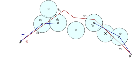
Figure 3: The path $\pi$ (in red) is a generalized path from $x$ to $y$. In blue, a polygonal path $\pi^{\prime}$ from $x$ to $y$ such that $T_{\varepsilon}(\pi^{\prime})\leq T_{\varepsilon}(\pi)$.

Let denote by $(a_{i},1\leq i\leq k)$ the first point of $[\pi]$ in $\mathcal{C}_{i}$ and $(b_{i},1\leq i\leq k)$ its last point (see Figure 3). Then we have

$$T_{\varepsilon}(\pi)=\sum_{i=0}^{k}N(a_{i+1}-b_{i})$$

with the convention $x=b_{0}$ and $y=a_{k+1}$. Let $c_{i}\in\Sigma\cap\mathcal{C}_{i}$ such that $a_{i}\in\partial B_{N}(c_{i},\varepsilon^{1/d}/2)$ and $d_{i}\in\Sigma\cap\mathcal{C}_{i}$ such that $b_{i}\in\partial B_{N}(c_{i},\varepsilon^{1/d}/2)$. Let $\pi_{i}=(c_{i},x_{i,1},\ldots,x_{i,n_{i}},d_{i})$ be a polygonal path (i.e., with vertices in $\Xi$) from $c_{i}$ to $d_{i}$ which remains in $\mathcal{C}_{i}$. Consider now the path $\pi^{\prime}$ from $x$ to $y$ which is the concatenation of the paths $(\pi_{i},1\leq i\leq k)$, namely

$$\pi^{\prime}:=(x,c_{1},x_{1,1},\ldots,x_{1,n_{1}},d_{1},c_{2},\ldots,d_{k},y).$$

By construction $\pi^{\prime}\in\Pi(x,y)$ and

$$T_{\varepsilon}(\pi^{\prime}) = N([x,c_{1}]\cap\Sigma_{\varepsilon}^{c})+N([d_{k},y]\cap\Sigma_{\varepsilon}^{c})+\sum_{i=1}^{k-1}N([d_{i},c_{i+1}]\cap\Sigma_{\varepsilon}^{c})$$ (26)

$$\leq N(c_{1}-x)-\frac{\varepsilon^{1/d}}{2}+N(y-d_{k})-\frac{\varepsilon^{1/d}}{2}+\sum_{i=1}^{k-1}\left(N(c_{i+1}-d_{i})-\varepsilon^{1/d}\right).$$

But, by triangle inequality, we have

$$N(c_{i+1}-d_{i})\leq N(b_{i}-d_{i})+N(a_{i+1}-b_{i})+N(c_{i+1}-a_{i+1})=\varepsilon^{1/d}+N(a_{i+1}-b_{i})\,,$$

and

$$N(c_{1}-x)\leq N(a_{1}-x)+\frac{\varepsilon^{1/d}}{2}\qquad\textrm{and}\qquad N(y-d_{k})\leq N(y-b_{k})+\frac{\varepsilon^{1/d}}{2}.$$

So we get that $T_{\varepsilon}(\pi^{\prime})\leq T_{\varepsilon}(\pi)$ as wanted.

∎

The next step is now to prove the existence of geodesics and of a time constant for this model. However, the proofs are more classical in this case than for the model with rewards. Indeed, the random variables $(\tilde{T}_{\varepsilon}(x,y),x,y\in\mathbb{R}^{d})$ are the travel times in a first passage percolation model, in particular, they are non negative, satisfy the triangle inequality and are bounded by $N(y-x)$. A classical use of Kingman’s subadditive ergodic theorem enables then to prove the existence of the time constant: for every $z\in\mathbb{R}^{d}$, there exists a constant $\tilde{\mu}_{\varepsilon}(z)\in[0,N(z)]$ such that

$$\lim_{s\rightarrow\infty}\frac{\tilde{T}_{\varepsilon}(0,sz)}{s}=\tilde{\mu}_{\varepsilon}(z)\quad\textrm{ a.s. and in }L^{1}.$$

Besides, the Euclidean case $N:=\|\cdot\|_{2}$, has been studied in [10] where a condition is given to ensure that $\tilde{\mu}_{\varepsilon}(\cdot):=\tilde{\mu}_{2,\varepsilon}(\cdot)$ is strictly positive in terms of a percolation event for the Boolean model $\Sigma_{\|\cdot\|_{2},\varepsilon}$. This result implies in particular that $\tilde{\mu}_{2,\varepsilon}(\cdot)$ is a norm for small enough $\varepsilon$. Using the equivalence of the norm on $\mathbb{R}^{d}$, we have that $\Sigma_{N,\varepsilon}\subset\Sigma_{\|\cdot\|_{2},c\varepsilon}$ for some $c>0$ so it is easy to deduce that, in fact, for any norm $N$, the function $\tilde{\mu}_{N,\varepsilon}(\cdot)$ is strictly positive for small enough $\varepsilon$. When $\tilde{\mu}_{\varepsilon}:=\tilde{\mu}_{N,\varepsilon}(\cdot)$ is a norm, a shape theorem also holds:

$$\mbox{for any $\delta>0$, for $t$ large enough }\quad\{z\in\mathbb{R}^{d},\tilde{T}_{\varepsilon}(0,z)\leq t\}\subset(1+\delta)B_{\tilde{\mu}_{\varepsilon}}(1)\mbox{ a.s.}$$

where $B_{\tilde{\mu}_{\varepsilon}}(1)$ denotes the unit ball for the norm $\tilde{\mu}_{\varepsilon}$. This implies in particular that for any $n\in\mathbb{N}$ and any $x,y\in B_{N}(n)$, there exists a.s. some $K>0$ such that

$$\tilde{T}_{\varepsilon}(x,y):=\inf\{\tilde{T}_{\varepsilon}(\pi)\,:\,\pi\in\Pi(x,y)\}=\min\{\tilde{T}_{\varepsilon}(\pi)\,:\,\pi\in\Pi(x,y),\pi\subset B_{N}(K)\}\,,$$

since the last set of paths is a.s. finite. This gives the existence, for any $x,y\in\mathbb{R}^{d}$, of a geodesic $\gamma_{\varepsilon}(x,y)\in\Pi(x,y)$, i.e., a polygonal path such that

$$\tilde{T}_{\varepsilon}(x,y)=\tilde{T}_{\varepsilon}(\gamma_{\varepsilon}(x,y)).$$

Of course, such geodesic is not unique since we can modify it inside any connected component of $\Sigma_{\varepsilon}$. To compare the model with rewards and the first passage percolation model, we will need in fact more properties on the geodesics we consider. So we introduce here a third set of paths, namely $\check{\Pi}_{\varepsilon}(x,y)$, and prove that the geodesics can be chosen inside this set. For a path $\pi=(x=x_{0},x_{1},\dots,x_{n}=y)$ from $x$ to $y$, let denote by $(\mathcal{C}_{1},\ldots,\mathcal{C}_{k})$ the connected component of $\Sigma_{\varepsilon}$ that the curve $[\pi]$ intersects. Define $\check{\Pi}_{\varepsilon}(x,y)$ as the set of paths from $x$ to $y$ such that

• $\pi\in\Pi(x,y)$.

• When $[\pi]$ exits a connected component of $\Sigma_{\varepsilon}$ it never enters it again.

• for every connected component $\mathcal{C}_{i}$, the subpath $[\pi]\cap\mathcal{C}_{i}$ can be written as $\pi_{i}=(a_{i},x_{i,0},\dots,x_{i,m_{i}},b_{i})$ where $m_{i}\geq 0$, $a_{i}$ (resp. $b_{i}$) is in the boundary of $\mathcal{C}_{i}$ and $B_{N}(x_{i,0},\varepsilon^{1/d}/2)$ (resp. $B_{N}(x_{i,m_{i}},\varepsilon^{1/d}/2)$) and for every $j\in\{0,\dots,m_{i}-1\}$, $N(x_{i,j+1}-x_{i,j})\leq\varepsilon^{1/d}$.

We emphasize that we impose that $m_{i}\geq 0$ in the third point. This means that each time the path enters a connected component $\mathcal{C}$ of $\Sigma_{\varepsilon}$, it gets at least trough one point of $\Xi\cap\mathcal{C}$.

Proposition 18.

For $\varepsilon$ small enough there exists a.s., for every $x,y\in\mathbb{R}^{d}$, a path $\check{\gamma}_{\varepsilon}(x,y)\in\check{\Pi}_{\varepsilon}(x,y)$ such that

$$\tilde{T}_{\varepsilon}(x,y)=\tilde{T}_{\varepsilon}(\check{\gamma}_{\varepsilon}(x,y))\,.$$

Proof.

Consider $\pi\in\hat{\Pi}(x,y)$ a geodesic between $x$ and $y$. We have already noticed that such path necessarily satisfies Point (ii) of the definition of $\check{\Pi}_{\varepsilon}(x,y)$. We construct now of new path $\pi^{\prime}$ between $x$ and $y$ in the exact same way than in proof of Proposition 17 except that we impose moreover that the polygonal subpath $\pi_{i}=(c_{i},x_{i,1},\ldots,x_{i,n_{i}},d_{i})$ created inside $\mathcal{C}_{i}$ between $c_{i}$ and $d_{i}$ satisfies $N(x_{i,j+1}-x_{i,j})\leq\varepsilon^{1/d}$ (such sequence of points necessarily exists since $\mathcal{C}_{i}$ is a connected component of balls of diameter $\varepsilon^{1/d}$). Besides, since $\pi$ is a geodesic, we necessarily have $T_{\varepsilon}(\pi)=T_{\varepsilon}(\pi^{\prime})$ so in particular, Inequality (26) must be an equality. This implies that $[\pi^{\prime}]$ cannot intersects other connected components of $\Sigma_{\varepsilon}$ than the one already intersected by $\pi$. So we deduce that each time $\pi^{\prime}$ enters a connected component $\mathcal{C}$ of $\Sigma_{\varepsilon}$, it get at least trough one point of $\Xi\cap\mathcal{C}$. Hence, $\pi^{\prime}$ is indeed a path of $\check{\Pi}_{\varepsilon}(x,y)$. ∎

6.2 Comparison between $\tilde{\mu}_{\varepsilon}(u)$ and $\mu_{\varepsilon}(u)$

The comparison between $\tilde{\mu}_{\varepsilon}(u)$ and $\mu_{\varepsilon}(u)$ is made in two steps. The first and easy step is to notice that, by looking at nice geodesics for the model with balls, we can prove that $\tilde{T}_{\varepsilon}(0,x)\geq T_{\varepsilon}(0,x)$ for every $x$, thus $\tilde{\mu}_{\varepsilon}(u)\leq\mu_{\varepsilon}(u)$. In the second step, we have to prove that $\tilde{T}_{\varepsilon}(0,x)-T_{\varepsilon}(0,x)$ is not too big. When a path $\pi=(0,x_{1},\dots,x_{n})$ goes through points $(x_{i})$ of $\Xi$ that are at $N$-distance bigger than $\varepsilon^{1/d}$, the corresponding balls of the Boolean model do not overlap, thus $\tilde{T}_{\varepsilon}(\pi)\leq T_{\varepsilon}(\pi)$. The travel time $\tilde{T}_{\varepsilon}(\pi)$ may be larger than $T_{\varepsilon}(\pi)$ only if $\pi$ goes through balls of the Boolean model that overlap. The difference $\tilde{T}_{\varepsilon}(\pi)-T_{\varepsilon}(\pi)$ can thus be controlled for a path $\pi=(0,x_{1},\dots,x_{n})$ by obtaining an upper bound on the numbers of couples of points among the $(x_{i})$ that are at $N$-distance less than $\varepsilon^{1/d}$ (see Inequality (28)). This upper bound is proved through Lemmas 19 and 20, using ideas that are quite similar to the ones used in Section 5.

By Proposition 18, for all $x\in\mathbb{R}^{d}$,we know that there exists a geodesic $\tilde{\gamma}_{\varepsilon}(x)=(0=x_{0},\ldots,x_{n}=x)\in\check{\Pi}_{\varepsilon}(0,x)$ for $\tilde{T}_{\varepsilon}(0,x)$ such that, for all $0<i<n$, $x_{i}\in\Xi$ and if $x_{i}$ and $x_{i+1}$ are in the same connected component of $\Sigma_{\varepsilon}$, $N(x_{i+1}-x_{i})\leq\varepsilon^{1/d}$. Let $(\mathcal{C}_{1},\dots,\mathcal{C}_{k})$ be the distinct connected components of $\Sigma_{\varepsilon}$ that the curve $[\tilde{\gamma}_{\varepsilon}(x)]$ intersects, and write $[\tilde{\gamma}_{\varepsilon}(x)]\cap\mathcal{C}_{i}=(a_{i},x_{i,0},\dots,x_{i,m_{i}},b_{i})$ as in property $(iii)$ of the definition of $\check{\Pi}_{\varepsilon}(0,x)$. Then

$$N(\tilde{\gamma}_{\varepsilon}(x)\cap\Sigma_{\varepsilon})=\sum_{i=1}^{k}N(\tilde{\gamma}_{\varepsilon}(x)\cap\mathcal{C}_{i})$$

and

$$N(\tilde{\gamma}_{\varepsilon}(x)\cap\mathcal{C}_{i})=\frac{\varepsilon^{1/d}}{2}+\sum_{j=0}^{m_{i}-1}N(x_{i,j+1}-x_{i,j})+\frac{\varepsilon^{1/d}}{2}\leq(m_{i}+1)\varepsilon^{1/d}\,.$$

We get that

$$N(\tilde{\gamma}_{\varepsilon}(x)\cap\Sigma_{\varepsilon})\leq\varepsilon^{1/d}\sharp\tilde{\gamma}_{\varepsilon}(x)$$ (27)

thus

$$\tilde{T}_{\varepsilon}(0,x)\geq T_{\varepsilon}(0,x).$$

This already yields that $\tilde{\mu}_{\varepsilon}(u)\geq\mu_{\varepsilon}(u)$.

Let now find an upper bound for $\tilde{\mu}_{\varepsilon}(u)-\mu_{\varepsilon}(u)$. For any polygonal path $\pi=(x_{0},\ldots,x_{q+1})$ with $x_{i}\in\Xi$ for $1\leq i\leq q$, we define

$$Y(\pi):=\{j\in\llbracket 1\,:\,q+1\rrbracket,\exists i<j,N(x_{j}-x_{i})\leq\varepsilon^{1/d}\}\,.$$

Note that if $j\notin Y(\pi)$, then $B_{N}(x_{j},\varepsilon^{1/d}/2)$ does not intersect any other ball $B_{N}(x_{i},\varepsilon^{1/d}/2)$ with $i<j$. Hence, we see that

$$\tilde{T}(\pi)\leq N(\pi)-\varepsilon^{1/d}(q-1-\mbox{card}(Y(\pi)))\leq T(\pi)+\varepsilon^{1/d}(2+\mbox{card}(Y(\pi))).$$

Applying this inequality to the geodesic $\gamma_{\varepsilon}(su)$ from $0$ to $su$ in the model with rewards studied previously, we get

$$\tilde{T}(\gamma_{\varepsilon}(su))\leq T(\gamma_{\varepsilon}(su))+\varepsilon^{1/d}(2+\mbox{card}(Y(\gamma_{\varepsilon}(su)))).$$ (28)

We obtain an upper bound for $\mbox{card}(Y(\gamma_{\varepsilon}(su)))$ by proving the following two lemmas.

Lemma 19.

For $\pi=(x_{0},\ldots,x_{q+1})$ a path let define

$$Z(\pi):=\{j\in\llbracket 1\,:\,q+1\rrbracket,N(x_{j}-x_{j-1})\leq 5\varepsilon^{1/d}\}.$$

Then we have a.s. for any geodesic $\gamma$, $\mbox{card}(Y(\gamma))\leq 2\mbox{card}(Z(\gamma))$.

Lemma 20.

Let $C_{2}$ be such that Theorem 3 holds. Fix some direction $u$ and some supporting plane $H$ of $B_{N}$ at $u$. Then, for any $\lambda>0$, there exists $\varepsilon_{0}>0$ thus that for $\varepsilon<\varepsilon_{0}$, we have, a.s. for $s$ large enough,

$$\mbox{card}(Z(\gamma_{\varepsilon}(su)))\leq\lambda g_{u}(C_{2}\varepsilon^{-1})\varepsilon^{-1/d}s.$$

Assuming these lemmas hold, we get that for any $\lambda>0$, for $\varepsilon$ small enough we have a.s. for $s$ large enough,

$$\tilde{T}(\gamma_{\varepsilon}(su))\leq T(\gamma_{\varepsilon}(su))+(2\varepsilon^{1/d}+2\lambda g_{u}(C_{2}\varepsilon^{-1})s)$$

which implies that

$$\limsup_{\varepsilon\to 0}\frac{\tilde{\mu}_{\varepsilon}(u)-\mu_{\varepsilon}(u)}{g_{u}(C_{2}\varepsilon^{-1})}\leq 2\lambda$$

and so Theorem 4 $(iii)$ holds.

Proof of Lemma 19.

To prove this inequality between the cardinal of $Y(\pi)$ and $Z(\pi)$, we in fact prove that

$$\mbox{card}(Y(\pi)\setminus Z(\pi))\leq\mbox{card}(Z(\pi)).$$

Let us first note that for a path $\pi=(0,x_{1},\ldots,x_{q})$ with $x_{i}\in\Xi$ for $1\leq i\leq q$, we have a.s. (since $0\notin\Xi$ a.s.)

$$T_{\varepsilon}(\pi)=\sum_{i=1}^{q}\left(N(x_{i}-x_{i-1})-\varepsilon^{1/d}\right)\,.$$

Thus if $T_{\varepsilon}(\pi)\leq-K\varepsilon^{1/d}$ it implies in particular that $\mbox{card}(Z(\pi))\geq K$. Let now $\gamma=(0,x_{1},\ldots,x_{q},x)$ be a finite geodesic from $0$ to $x$ for $T_{\varepsilon}$ and let $j(1)<\ldots<j(l)$ the indices such that

$$Y(\gamma)\setminus Z(\gamma)=\{x_{j(1)},\ldots,x_{j(l)}\}.$$

Let define, for $i\leq q$, the truncated path $\gamma_{i}=(0,x_{1},\ldots,x_{i})$. Let us prove by induction on $i$ that

$$\mbox{card}(Z(\gamma_{j(i)}))\geq i$$ (29)

which would imply that

$$\mbox{card}(Z(\gamma))\geq\mbox{card}(Z(\gamma_{j(l)}))\geq l=\mbox{card}(Y(\gamma)\setminus Z(\gamma))\,.$$

We have by definition $x_{j(1)}\in Y(\gamma)\setminus Z(\gamma)$, i.e., there exists some $k<j(1)$ such that $N(x_{j(1)}-x_{k})\leq\varepsilon^{1/d}$ but $N(x_{j(1)}-x_{j(1)-1})\geq 5\varepsilon^{1/d}$. Using that

$$\varepsilon^{1/d}\geq N(x_{k}-x_{j(1)})\geq T_{\varepsilon}(x_{k},x_{j(1)})=T_{\varepsilon}(x_{k},x_{j(1)-1})+T_{\varepsilon}(x_{j(1)-1},x_{j(1)})\geq T_{\varepsilon}(x_{k},x_{j(1)-1})+3\varepsilon^{1/d}$$

we get that

$$T_{\varepsilon}(x_{k},x_{j(1)-1})\leq-2\varepsilon^{1/d}$$

which implies in particular that

$$\mbox{card}(Z(\gamma_{j(1)}))\geq\mbox{card}(Z((x_{k},\ldots,x_{j(1)-1})))\geq 1.$$

Fix $i$, and assume now that for every $m<i$, we have $\mbox{card}(Z(\gamma_{j(m)}))\geq m$. Let $k<j(i)$ such that $N(x_{j(i)}-x_{k})\leq\varepsilon^{1/d}$. Let $m<i$ such that $j(m)<k\leq j(m+1)$ with the convention $j(0)=0$. We have

$$\varepsilon^{1/d}\geq T_{\varepsilon}(x_{k},x_{j(i)})=T_{\varepsilon}(x_{k},x_{j(m+1)-1})+\sum_{p=m+1}^{i}T_{\varepsilon}(x_{j(p)-1},x_{j(p)})+\sum_{p=m+1}^{i-1}T_{\varepsilon}(x_{j(p)},x_{j(p+1)-1})\,.$$

By definition of the indexes $j(p)$, we have $T_{\varepsilon}(x_{j(p)-1},x_{j(p)})\geq 3\varepsilon^{1/d}$ so we get

$$T_{\varepsilon}(x_{k},x_{j(m+1)-1})+\sum_{p=m+1}^{i-1}T_{\varepsilon}(x_{j(p)},x_{j(p+1)-1})\leq\varepsilon^{1/d}(1-3(i-m))\leq-2(i-m)\varepsilon^{1/d}\,.$$

This implies in particular that

$$\mbox{card}(Z((x_{k},\ldots,x_{j(i)})))\geq i-m$$

for some $k\geq j(m)$. But, by hypothesis, we have

$$\mbox{card}(Z((0,\ldots,x_{k-1})))\geq\mbox{card}(Z((0,\ldots,x_{j(m)})))\geq m$$

so we get

$$\mbox{card}(Z(\gamma_{j(i)}))\geq i\,.$$

∎

Proof of Lemma 20.

Fix some $C_{2}$ such that Theorem 3 holds. Fix some $\lambda>0$. Setting $\eta_{\infty}:=g_{u}(C_{2}\varepsilon^{-1})$, we want to prove that for $\varepsilon$ small enough, we have, a.s. for $s$ large enough

$$\mbox{card}(Z(\gamma_{\varepsilon}(su)))\leq\lambda\eta_{\infty}\varepsilon^{-1/d}s.$$

Recall that we have a.s. for $s$ large enough $N(\gamma_{\varepsilon}(su))\leq s(1+2\eta_{\infty})$ and $\sharp\gamma_{\varepsilon}(su)\leq 2\eta_{\infty}\varepsilon^{-1/d}s$. Thus, it is sufficient to show that for $s$ large enough, for any path $\pi$ from $0$ to $su+H$ such that $N(\pi)\leq s(1+2\eta_{\infty})$ and $\sharp\pi\leq 2\eta_{\infty}\varepsilon^{-1/d}s$ , we have

$$\sharp Z(\pi)\leq\lambda\eta_{\infty}\varepsilon^{-1/d}s.$$

Let $q_{0}:=\lambda\eta_{\infty}\varepsilon^{-1/d}s$, $q_{1}:=2\eta_{\infty}\varepsilon^{-1/d}s$, $\eta:=2\eta_{\infty}$ and set

$$\mathcal{F}(s):=\{\exists\pi\in\Pi(0,su+H),N(\pi)\leq(1+\eta)s,\sharp\pi\leq q_{1},\;\mbox{card}(Z(\pi))\geq q_{0}\}.$$

Proving that $\mathcal{F}(s)$ does not occur a.s. for $s$ large enough will yield Lemma 20. To bound $\mathbb{P}(\mathcal{F}(s))$, we roughly use the same idea as in Section 5. For a sequence of points $(x_{i})_{1\leq i\leq q}$ in $\Xi$, let denote by $(t_{i})_{1\leq i\leq q}$ their increments, i.e., $t_{i}=x_{i}-x_{i-1}$ (with the convention $t_{1}=x_{1}$). Then, we have

$$\mathbb{P}[\mathcal{F}(s)]=\sum_{q\leq q_{1}}\sum_{Z\subset\{1,\ldots,q\},|Z|\geq q_{0}}\mathbb{P}(\mathcal{A}_{Z})$$

where

$$\mathcal{A}_{Z}:=\{\exists(x_{i})_{1\leq i\leq q}\in\Xi^{q},x_{q}\cdot u^{\star}\leq s,\sum_{i=1}^{q}N(t_{i})\leq\eta s+x_{q}\cdot u^{\star},\forall j\in Z,t_{j}\cdot u^{\star}\leq 5\varepsilon^{1/d}\}.$$

Using Chernov inequality, we have for all $\alpha,\beta>0$,

$$\mathbb{P} [\mathcal{A}_{Z}]$$

$$\leq\int_{(\mathbb{R}^{d})^{q}}\exp\left(\beta(s-x_{q}\cdot u^{\star})+\alpha(\eta s+x_{q}\cdot u^{\star}-\sum_{i=1}^{q}N(t_{i}))\right)\prod_{j\in Z}\exp\left(\frac{\alpha}{2}(4\varepsilon^{1/d}-(t_{j}\cdot u^{\star}))\right)dt_{1}\ldots dt_{q}\,.$$

Taking $\beta=\alpha\eta$, we get

$$\mathbb{P}[\mathcal{A}_{Z}] \leq \exp(\alpha(2\eta s+2\varepsilon^{1/d}\mbox{card}(Z))\int_{(\mathbb{R}^{d})^{q}}\exp\left(-\alpha\sum_{i=1}^{q}\left[N(t_{i})-\left(1-\eta-\frac{1_{j\in Z}}{2}\right)(t_{i}\cdot u^{\star})\right]\right)dt_{1}\ldots dt_{q}$$

$$= \exp(2\alpha(\eta s+\varepsilon^{1/d}\mbox{card}(Z))\left(\frac{I(\eta)}{\alpha^{d}}\right)^{q-\mbox{card}(Z)}\left(\frac{I(\frac{1}{2}+\eta)}{\alpha^{d}}\right)^{\mbox{card}(Z)}$$

$$= \exp(2\alpha(\eta s+\varepsilon^{1/d}\mbox{card}(Z))\left(\frac{I(\eta)^{1-\mbox{card}(Z)/q}I(\frac{1}{2}+\eta)^{\mbox{card}(Z)/q}}{\alpha^{d}}\right)^{q}.$$

We know that $\lim_{\eta\to 0}I(\eta)=\lim_{\eta\to 0}h_{u}(\eta)=+\infty$ whereas $I(\eta)$ is bounded on $[1/2,1]$. Since $\eta_{\infty}$ tends to 0 as $\varepsilon$ tends to 0, we deduce that for $\varepsilon$ small enough, $I(\eta)\geq I(\frac{1}{2}+\eta)$ and so we get that for $\mbox{card}(Z)\geq q_{0}$ and $q\leq q_{1}$,

$$I(\eta)^{1-\mbox{card}(Z)/q}I\left(\frac{1}{2}+\eta\right)^{\mbox{card}(Z)/q} \leq I(\eta)^{1-q_{0}/q_{1}}I\left(\frac{1}{2}+\eta\right)^{q_{0}/q_{1}}$$

$$=I(\eta)^{1-\lambda/2}I\left(\frac{1}{2}+\eta\right)^{\lambda/2}$$

$$\leq c_{1}I(2\eta_{\infty})^{1-\lambda/2}$$

for $\lambda\in(0,1)$ and $c_{1}:=\sup\{I(x),x\in[1/2,1]\}\vee 1$. Using (11) in Lemma 10, which states that $I$ is of the same order than $h_{u}$ near 0, we also get, for some constant $c_{2}$, for $\varepsilon$ small enough,

$$I(2\eta_{\infty})\leq c_{2}h_{u}(2\eta_{\infty})\leq c_{2}h_{u}(\eta_{\infty})=c_{2}C_{2}\varepsilon^{-1}.$$

So we get, for some constant $c_{3}>0$,

$$\mathbb{P}[\mathcal{F}(s)] \leq \sum_{q_{0}\leq q\leq q_{1}}2^{q}\exp(2\alpha(2\eta_{\infty}s+\varepsilon^{1/d}q_{1})\left(\frac{c_{3}\varepsilon^{-1+\lambda/2}}{\alpha^{d}}\right)^{q}.$$

$$\leq \sum_{q\geq q_{0}}\exp(8\alpha\eta_{\infty}s)\left(\frac{2c_{3}\varepsilon^{-1+\lambda/2}}{\alpha^{d}}\right)^{q}$$

Taking $\alpha^{d}=4c_{3}\varepsilon^{-1+\lambda/2}$, i.e., $\alpha=c_{4}\varepsilon^{-(1/d)+\lambda/(2d)}$, we obtain

$$\mathbb{P}[\mathcal{F}(s)] \leq 2\exp(8c_{4}\varepsilon^{-(1/d)+\lambda/(2d)}\eta_{\infty}s-q_{0}\log 2)$$

$$= 2\exp(-s\varepsilon^{-1/d}\eta_{\infty}(\lambda\log 2-8c_{4}\varepsilon^{\lambda/(2d)})).$$

Hence, for any $\lambda\in(0,1)$, if $\varepsilon$ is small enough, this quantity decreases to 0 exponentially fast in $s$. Taking

$$s_{n}:=n\varepsilon^{1/d}/(\lambda\eta_{\infty})$$

Borel-Cantelli Lemma yields that there exists a.s. $n_{0}$ such that, for $n\geq n_{0}$, $\mathcal{F}(s_{n})$ does not occur. Since for $s\in[s_{n},s_{n+1}[$, $\lfloor\lambda\eta_{\infty}\varepsilon^{-1/d}s\rfloor=\lfloor\lambda\eta_{\infty}\varepsilon^{-1/d}s_{n}\rfloor$, we deduce using the same argument as in proof of Proposition 13, that in fact $\mathcal{F}(s)$ does not occur for $s$ large enough.

∎

6.3 Proof of the lower bound on $1-\tilde{\mu}_{\varepsilon}(u)$

When $1-\mu_{\varepsilon}(u)$ is of order $g_{u}(C_{2}\varepsilon^{-1})$ when $\varepsilon$ goes to $0$, it is a straightforward consequence of Theorem 4 $(iii)$ that the same holds for $1-\tilde{\mu}_{\varepsilon}(u)$. It will be the case for specific choices of the norm $N$, namely the $p$-norms, see Section 7. However, in general setting, the lower bound on $1-\mu_{\varepsilon}(u)$ given by Theorem 3 is $\bar{g}_{u}(C_{1}\varepsilon^{-1})$, and there is no way to deduce the same lower bound for $1-\tilde{\mu}_{\varepsilon}(u)$ through Theorem 4 $(iii)$. It is however easy to adapt the greedy algorithm used to prove the lower bound on $1-\mu_{\varepsilon}(u)$ in Section 4 to get the same type of lower bound on $1-\tilde{\mu}_{\varepsilon}(u)$. The idea is to add an extra space between two consecutive points of the process $\Xi$ that are collected by the greedy algorithm, to make sure that the corresponding balls of diameter $\varepsilon^{1/d}$ in the Boolean model do not intersect. Let us get into details.

Fix a direction $u\in\mathbb{R}^{d}$ with $N(u)=1$, $H$ a supporting hyperplane of $B_{N}(1)$ at $u$ and recall that

$$M_{\eta}:=\{v\in H\,:\,N(u+v)\leq 1+\eta\mbox{ and }N(u-v)\leq 1+\eta\}\qquad\textrm{and}\qquad\bar{h}_{u}(\eta):=\eta^{-d}|M_{\eta}(u)|\,.$$

We state the following analog of Proposition 11.

Proposition 21.

There exists a constant $c^{\prime}>0$ (depending only on $d,N$) such that, for all direction $u\in\mathbb{R}^{d}$ with $N(u)=1$, for all $\eta\in(0,1)$, we have

$$\tilde{\mu}_{\varepsilon}(u)\leq 1+\eta-c^{\prime}\varepsilon^{1/d}|M_{\eta}|^{1/d}\,.$$

In particular, we have, with $C_{1}^{\prime}:=\left(\dfrac{2}{c^{\prime}}\right)^{d}$,

$$\tilde{\mu}_{\varepsilon}(u)\leq 1-\bar{g}_{u}(C^{\prime}_{1}\varepsilon^{-1})\,.$$

Proof.

We use almost the same greedy algorithm as in the proof of Proposition 11 except that we impose also that two consecutive points taken by the greedy path must be at distance at least $1$. Recall that for $s\geq 0$

$$C_{\eta}(s) :=\{x=\lambda u+v\,:\,0\leq\lambda\leq s\,,\,v\in H\,,\,N(\lambda u+v)\leq\lambda(1+\eta),N(\lambda u-v)\leq\lambda(1+\eta)\}\,,$$

and we have

$$|C_{\eta}(s)|=\frac{1}{d\|u^{\star}\|_{2}}|M_{\eta}|s^{d}\,.$$

Recall that $\Xi$ denotes the points of a Poisson point process with unit intensity on $\mathbb{R}^{d}$. By induction we define a sequence $(X_{n})_{n\geq 0}$ in $\mathbb{R}^{d}$ with $X_{0}=0$ and if

$$\lambda_{n+1}:=\inf\{s>1\,:\,(X_{n}+C_{\eta}(s))\cap\Xi\neq\emptyset\}$$

(we emphasize the fact that we require that $s>1$), we set $X_{n+1}=X_{n}+\lambda_{n+1}u+W_{n+1}$ with $W_{n+1}\in H$ and such that $X_{n+1}=(X_{n}+C_{\eta}(\lambda_{n+1}))\cap\Xi$. We define $S_{n}=\sum_{i=1}^{n}\lambda_{i}$ and $V_{n}=\sum_{i=1}^{n}W_{i}$. By the properties of Poisson point processes, $(\lambda_{i})_{i\geq 1}$ and $(W_{i})_{i\geq 1}$ are i.i.d. random variables and since $M_{\eta}(u)$ is a symmetric set, $W_{1}$ has also a symmetric distribution and so $V_{n}$ is a symmetric random walk.

Let us now define, for $s>0$,

$$Z(s):=\sup\{n\geq 0\,:\,S_{n}\leq s\}$$

and consider the path $\pi_{s}=(0,X_{1},\dots,X_{Z(s)},su)$. Let us find an upper bound of $\tilde{T}_{\varepsilon}(\pi_{s})$ by finding an upper bound of its length and a lower bound of $Z(s)$, its number of points.

The sequence $(\lambda_{i})_{i\geq 1}$ is i.i.d. and we have for $t\geq 1$,

$$\mathbb{P}(\lambda_{1}\geq t) =\exp\left(-\frac{1}{d\|u^{\star}\|_{2}}|M_{\eta}(u)|(t^{d}-1)\right)$$

so that

$$\mathbb{E}(\lambda_{1}) =1+\int_{1}^{\infty}\exp\left(-\frac{1}{d\|u^{\star}\|_{2}}|M_{\eta}(u)|(t^{d}-1)\right)du$$

$$=1+\left(\frac{|M_{\eta}(u)|}{d\|u^{\star}\|_{2}}\right)^{-1/d}\int_{(|M_{\eta}(u)|/\|u^{\star}\|_{2})^{1/d}}^{\infty}\exp(-v^{d})dv:=1+\frac{|M_{\eta}(u)|^{-1/d}}{2c^{\prime}_{u}}$$

where

$$2c^{\prime}_{u}:=\left(\frac{1}{d\|u^{\star}\|_{2}}\right)^{1/d}\left(\int_{(|M_{\eta}(u)|/\|u^{\star}\|_{2})^{1/d}}^{\infty}\exp(-v^{d})dv\right)^{-1}\,.$$

Using that for any $\eta\in(0,1)$, $M_{\eta}(u)\subset B_{N}(0,3)$ we see that the $(d-1)$-dimensional volume $|M_{\eta}(u)|$ of $M_{\eta}(u)$ is bounded by some constant $c_{1}^{\prime}$ (depending only on $d$ and $N$) for $\eta\in(0,1)$. By Lemma 9, we also know that $c\leq\|u^{\star}\|_{2}\leq c^{\prime}$ for constants $c,c^{\prime}\in(0,\infty)$ (depending only on $d$ and $N$). We deduce that there exist some constants $c_{2},c_{3}>0$ (depending only on $d$ and $N$ also) such that for $\eta\in(0,1)$,

$$c_{2}|M_{\eta}|^{-1/d}\leq\mathbb{E}(\lambda_{1})\leq c_{3}|M_{\eta}|^{-1/d}\,.$$

Since $S_{n}=\sum_{i=1}^{n}\lambda_{i}$, a standard renewal theorem yields that, setting $c_{4}=1/(2c_{3})$ and $c_{5}=2/c_{2}$, for $s$ large enough, we have a.s.

$$c_{4}|M_{\eta}|^{1/d}s\leq Z(s)\leq c_{5}|M_{\eta}|^{1/d}s\,.$$ (30)

This gives a lower bound for the number of points in $\pi_{s}$. The rest of the proof of Proposition 21 is a copy of the proof of Proposition 11 with Equation (30) instead of (15). ∎

6.4 Upper bound on $N(\tilde{\gamma}_{\varepsilon}(su))$

We recall that $\tilde{\gamma}_{\varepsilon}(su)\in\hat{\Pi}(0,su)$ designates a generalized path that is a geodesic for $\tilde{T}_{\varepsilon}(0,su)$ and has minimal $N$-length. To complete the proof of Theorem 4, it remains to prove $(ii)$,i.e., the upper bound on $N(\tilde{\gamma}_{\varepsilon}(su))$. In fact, if $\check{\gamma}_{\varepsilon}(su)\in\check{\Pi}_{\varepsilon}(0,su)$ designates a path that is a geodesic for $\tilde{T}_{\varepsilon}(0,su)$, then $\check{\gamma}_{\varepsilon}(su)\in\hat{\Pi}(0,su)$ too and by minimality we know that $N(\tilde{\gamma}_{\varepsilon}(su))\leq N(\check{\gamma}_{\varepsilon}(su))$. We will in fact prove an upper bound for $N(\check{\gamma}_{\varepsilon}(su))$. Since $\check{\gamma}_{\varepsilon}(su)\in\check{\Pi}_{\varepsilon}(0,su)$, Equation (27) states that

$$N(\check{\gamma}_{\varepsilon}(su)\cap\Sigma_{\varepsilon})\leq\varepsilon^{1/d}\sharp\check{\gamma}_{\varepsilon}(su)$$

which gives that

$$N(\check{\gamma}_{\varepsilon}(su))\leq\tilde{T}(\check{\gamma}_{\varepsilon}(su))+\varepsilon^{1/d}\sharp\check{\gamma}_{\varepsilon}(su)\leq s+\varepsilon^{1/d}\sharp\check{\gamma}_{\varepsilon}(su).$$

One can check that the proof of (21) (which gives an upper bound for the length and the number of points of the geodesic in the model with rewards) only use a similar inequality between $N(\gamma_{\varepsilon}(su))$ and $\sharp\gamma_{\varepsilon}(su)$. Mimicking this proof, we can so also obtain that, for any $\delta>1$,

$$N(\check{\gamma}_{\varepsilon}(su))\leq s(1+\delta g_{u}(C_{2}\varepsilon^{-1}))\textrm{ and }\sharp\check{\gamma}_{\varepsilon}(su)\leq\delta g_{u}(C_{2}\varepsilon^{-1})\varepsilon^{-1/d}s.$$ (31)

7 $p$-norm

In this section, we suppose that $N$ is the $p$-norm for some $p\in[1,\infty]$. We put a subscript $p$ in our notations to emphasize the dependence on $p$. For a given $u\in\mathbb{R}^{d}$, we recall that the definition of $d_{i}(u)$, $i\in\{1,\dots,4\}$ is given in (1.4). For a given $p\in[1,\infty]$ the definition of $\kappa_{p}(u)$ is given in (6).

This section is organized as follows. First in Section 7.1 we specify for each $p\in[1,\infty]$ and each $u\in\mathbb{R}^{d}$ such that $\|u\|_{p}=1$ what hyperplane $H$ we consider as a supporting hyperplane of $B_{p}(1)$ at $u$, and fix some notations. In this setting, we evaluate $|K_{\eta}(u)|$ in Section 7.2. This must be done separately for $p\in(1,\infty)$, $p=1$ and $p=+\infty$, since the estimations are based on a proper rescaling of $K_{\eta}(u)$ which is not exactly of the same nature in those different situations. Then in Section 7.3 we compare $|M_{\eta}(u)|$ to $|K_{\eta}(u)|$. This allows us to apply the results proved for a general norm $N$ to the $p$-norm in Section 7.4 to prove Theorems 5 and 6. Finally in Section 7.5 we prove Theorem 7, i.e., the existence of $\lim_{\varepsilon\rightarrow 0}(1-\mu_{\varepsilon}(u))/\varepsilon^{\kappa_{p}(u)}$, by an argument of monotonicity, at least for some $p$ and $u$.

7.1 Choice and description of the supporting hyperplane $H$

We have to deal separately with the cases $p\in(1,\infty)$, $p=1$ and $p=\infty$. From now on, until the end of Section 7, we always consider that the hyperplane $H$ we work with is the one described here.

Case $p\in(1,\infty)$.

Consider $N=\|\cdot\|_{p}$ for some $p\in(1,\infty)$. Let $u\in\mathbb{R}^{d}$ such that $\|u\|_{p}=1$. Let $d_{1}:=d_{1}(u)$ be the number of coordinates of $u$ that are not null. By invariance of the model under symmetries along the hyperplanes of coordinates and by permutations of coordinates, we can suppose that $u=(u_{1},\dots,u_{d_{1}},0,\dots,0)$ with $u_{i}>0$ for $i\in\{1,\dots,d_{1}\}$. The ball $B_{p}(1)$ is strictly convexe, and the (unique) supporting hyperplane $H$ of $B_{p}(1)$ at $u$ is

$$H:=\{v\in\mathbb{R}^{d}\,:\,v\cdot u^{\star}=0\}$$

where $u^{\star}=(u_{1}^{p-1},\ldots,u_{d_{1}}^{p-1},0,\ldots,0)$ satisfies $u\cdot u^{\star}=\sum_{i=1}^{d_{1}}u_{i}^{p}=1$ ($u^{\star}$ is the dual vector of $u$). Note that we have $H=H_{1}\oplus H_{2}$ where $H_{1}\subset\mbox{Vect}(e_{1},\ldots,e_{d_{1}})$ and $H_{2}=\mbox{Vect}(e_{d_{1}+1},\ldots,e_{d})$, for $(e_{1},\dots,e_{d})$ the canonical orthonormal basis of $\mathbb{R}^{d}$. For $v\in H$, we write $v=v_{1}+v_{2}$ with $v_{1}=(v_{1,1},\dots,v_{1,d_{1}},0,\dots,0)\in H_{1}$ and $v_{2}=(0\dots,0,v_{2,d_{1}+1},\dots,v_{2,d})\in H_{2}$.

Case $p=1$.

Consider $N=\|\cdot\|_{1}$ and let $u\in\mathbb{R}^{d}$ such that $\|u\|_{1}=1$. We can suppose that $u=(u_{1},\ldots,u_{d_{1}},0,\ldots,0)$ with $u_{i}>0$ for all $i\in\{1,\ldots,d_{1}\}$ with $d_{1}=d_{1}(u)$. In this case, a supporting hyperplane $H$ of $B_{1}(1)$ at $u$ is

$$H:=\{v\in\mathbb{R}^{d}\,:\,v\cdot u^{\star}=0\}$$

where $u^{\star}=(1,\ldots,1,0,\ldots,0)$ satisfies $u\cdot u^{\star}=\sum_{i=1}^{d_{1}}u_{i}=1$. We emphasize the fact that this hyperplane $H$ is not the unique supporting hyperplane of $B_{1}(1)$ at $u$ if $d_{1}<d$, but this is the most natural choice of supporting hyperplane since it is the most symmetric. As for $p\in(1,\infty)$, note that we have $H=H_{1}\oplus H_{2}$ where $H_{1}\subset\mbox{Vect}(e_{1},\ldots,e_{d_{1}})$ and $H_{2}=\mbox{Vect}(e_{d_{1}+1},\ldots,e_{d})$, for $(e_{1},\dots,e_{d})$ the canonical orthonormal basis of $\mathbb{R}^{d}$. For $v\in H$, we write $v_{1}=(v_{1,1},\dots,v_{1,d_{1}},0,\dots,0)\in H_{1}$ and $v_{2}=(0\dots,0,v_{2,d_{1}+1},\dots,v_{2,d})\in H_{2}$.

Case $p=\infty$.

Consider $N=\|\cdot\|_{\infty}$ and let $u\in\mathbb{R}^{d}$ such that $\|u\|_{\infty}=1$. We can suppose that $u=(1,\ldots,1,u_{d_{3}+1},\ldots,u_{d})$ with $u_{i}\in[0,1)$ for all $i\in\{d_{3}+1,\ldots,d\}$ with $d_{3}:=d_{3}(u)$. In this case, a supporting hyperplane $H$ of $B_{\infty}(1)$ at $u$ is

$$H:=\{v\in\mathbb{R}^{d}\,:\,v\cdot u^{\star}=0\}$$

where $u^{\star}=(1/d_{3},\ldots,1/d_{3},0,\ldots,0)$ (with $d_{3}$ non null coordinates) satisfies $u\cdot u^{\star}=\sum_{i=1}^{d_{3}}1/d_{3}=1$. We emphasize the fact that this hyperplane $H$ is not the unique supporting hyperplane of $B_{\infty}(1)$ at $u$ if $d_{3}>1$, but this is the most natural choice of supporting hyperplane since it is the most symmetric. Note that we have $H=H_{3}\oplus H_{4}$ where $H_{3}\subset\mbox{Vect}(e_{1},\ldots,e_{d_{3}})$ and $H_{4}=\mbox{Vect}(e_{d_{3}+1},\ldots,e_{d})$, for $(e_{1},\dots,e_{d})$ the canonical orthonormal basis of $\mathbb{R}^{d}$. For $v\in H$, we write $v_{3}=(v_{3,1},\dots,v_{3,d_{3}},0,\dots,0)\in H_{3}$ and $v_{4}=(0\dots,0,v_{4,d_{3}+1},\dots,v_{4,d})\in H_{4}$.

7.2 Evaluation of $|K_{\eta}(u)|$

The aim of this section is to prove the following estimate of $|K_{\eta}(u)|$.

Proposition 22.

Consider $N=\|\cdot\|_{p}$ for some $p\in[1,\infty]$. Let $u\in\mathbb{R}^{d}$ such that $\|u\|_{p}=1$ and $H$ the supporting hyperplane of $B_{p}(1)$ at $u$ as defined in Section 7.1. There exist two constants $A_{1}:=A_{1}(p,d,u)$, $A_{2}:=A_{2}(p,d,u)$, such that for any $\eta\in(0,1]$, we have

$$A_{1}\eta^{\gamma_{p}(u)}\leq|K_{\eta}(u)|\leq A_{2}\eta^{\gamma_{p}(u)}$$

with

$$\gamma_{p}(u):=\left\{\begin{array}[]{ll}\frac{d_{1}(u)-1}{2}+\frac{d_{2}(u)}{p}&\textrm{ if }p\in(1,\infty)\,,\\ d_{2}(u)=d-d_{1}(u)&\textrm{ if }p=1\,,\\ d_{3}(u)-1=d-(d_{4}(u)+1)&\textrm{ if }p=\infty\,.\end{array}\right.$$ (32)

The proof of Proposition 22 is based on the simple idea that $K_{\eta}(u)$, when properly rescaled with $\eta$, looks roughly like a Euclidean ball in $H$. However, the good rescaling depends on $p$, and has to be done in a specific way for $p=1$ and $p=\infty$.

7.2.1 $p$-norm with $p\in(1,\infty)$

The good rescaling in $\eta$ in this case is of order $\eta^{1/2}$ in $H_{1}$ whereas it is of order $\eta^{1/p}$ in $H_{2}$. We make it clear in the following lemma.

Lemma 23.

Let $p\in(1,\infty)$ and

$$\hat{K}_{\eta}(u):=\{v\in H\,:\,\|u+\eta^{1/2}v_{1}+\eta^{1/p}v_{2}\|_{p}^{p}\leq 1+\eta\}\,.$$

Then, there exist $\eta_{0}>0$, $R_{1}>R_{0}>0$ (depending on $p$, $d$ and $u$) such that, for all $\eta\in(0,\eta_{0})$,

$$B_{H}(R_{0})\subset\hat{K}_{\eta}(u)\subset B_{H}(R_{1})$$

where $B_{H}(r):=\{v\in H\,:\,\|v\|_{2}\leq r\}$.

Proof of Lemma 23.

Let us find $R_{0}$ such that $B_{H}(R_{0})\subset\hat{K}_{\eta}(u)$ for $\eta\in(0,1]$. We have

$$|1+t|^{p}=1+pt+O(t^{2})\,.$$

Thus, there exists $c>0$, such that, for all $t\in[-1,1]$,

$$|1+t|^{p}\leq 1+pt+ct^{2}.$$

Let $R$ be small enough such that $R\leq\min\{u_{i},i\leq d_{1}\}$ and $dR^{p}+cR^{2}\sum_{i\leq d_{1}}u_{i}^{p-2}\leq 1$. Let $v\in H$ such that $\|v\|_{\infty}\leq R$. Then

$$\|u+\eta^{1/2}v_{1}+\eta^{1/p}v_{2}\|_{p}^{p}=\eta\|v_{2}\|_{p}^{p}+\sum_{i\leq d_{1}}|u_{i}+\eta^{1/2}v_{1,i}|^{p}\,.$$

If $\eta\leq 1$, we have for all $1\leq i\leq d_{1}$,

$$\left\|\frac{\eta^{1/2}v_{1,i}}{u_{i}}\right\|\leq\frac{R}{u_{i}}\leq 1\,,$$

hence we have

$$|u_{i}+\eta^{1/2}v_{1,i}|^{p}\leq u_{i}^{p}+\eta^{1/2}p\,v_{1,i}\,u_{i}^{p-1}+\eta\,c\,v_{1,i}^{2}\,u_{i}^{p-2}\,.$$

Using that $v_{1}\cdot u^{\star}=0$ and $||u||_{p}=1$, we get

$$\|u+\eta^{1/2}v_{1}+\eta^{1/p}v_{2}\|_{p}^{p} \leq \eta d\|v_{2}\|_{\infty}^{p}+1+\eta c\sum_{i\leq d_{1}}v_{1,i}^{2}u_{i}^{p-2}$$

$$\leq 1+\eta\left(dR^{p}+cR^{2}\sum_{i\leq d_{1}}u_{i}^{p-2}\right)$$

$$\leq 1+\eta$$

which proves that $v\in\hat{K}_{\eta}(u)$. Using that $\|v\|_{2}\geq\|v\|_{\infty}$, we get that $B_{H}(R)\subset\hat{K}_{\eta}(u)$.

Let us now find $\eta_{0}>0$ and $R_{1}>0$ such that $\hat{K}_{\eta}(u)\subset B_{H}(R_{1})$ for $\eta\in(0,\eta_{0}]$. We have

$$|1+t|^{p}=1+pt+\frac{p(p-1)}{2}t^{2}+O(t^{3})\,.$$

Thus, there exists $c>0$ such that, for all $t\in\mathbb{R}$,

$$|1+t|^{p}\geq 1+pt+\frac{p(p-1)}{2}t^{2}-c|t|^{3}.$$

Let $R>0$ such that

$$\min\left(R^{p},\frac{p(p-1)}{2}R^{2}\min_{i\leq d_{1}}u_{i}^{p-2}\right)>2$$

and let $\eta_{0}>0$ such that $R^{3}\,c\,\eta_{0}^{1/2}\sum_{i\leq d_{1}}u_{i}^{p-3}=1$. Let $v\in H$ such that $\|v\|_{\infty}=R$. We have, for all $1\leq i\leq d_{1}$,

$$|u_{i}+\eta^{1/2}v_{1,i}|^{p}\geq u_{i}^{p}+\eta^{1/2}\,p\,v_{1,i}\,u_{i}^{p-1}+\eta\,\frac{p(p-1)}{2}\,v_{1,i}^{2}\,u_{i}^{p-2}-c\eta^{3/2}\,|v_{1,i}|^{3}\,u_{i}^{p-3}\,.$$

Using that $v_{1}\cdot u^{\star}=0$ and $\|u\|_{p}=1$, we get, for $\eta\in(0,\eta_{0})$

$$\|u+\eta^{1/2}v_{1}+\eta^{1/p}v_{2}\|_{p}^{p} \geq \eta\|v_{2}\|_{p}^{p}+1+\eta\,\frac{p(p-1)}{2}\sum_{i\leq d_{1}}v_{1,i}^{2}\,u_{i}^{p-2}-c\,\eta^{3/2}\sum_{i\leq d_{1}}|v_{1,i}|^{3}\,u_{i}^{p-3}$$

$$\geq 1+\eta\left(\|v_{2}\|_{\infty}^{p}+\frac{p(p-1)}{2}\|v_{1}\|_{\infty}^{2}\min_{i\leq d_{1}}u_{i}^{p-2}-\|v_{1}\|_{\infty}^{3}\,c\,\eta_{0}^{1/2}\sum_{i\leq d_{1}}u_{i}^{p-3}\right)$$

$$\geq 1+\eta\left(\|v_{2}\|_{\infty}^{p}+\frac{p(p-1)}{2}\|v_{1}\|_{\infty}^{2}\min_{i\leq d_{1}}u_{i}^{p-2}-R^{3}\,c\,\eta_{0}^{1/2}\sum_{i\leq d_{1}}u_{i}^{p-3}\right)$$

$$> 1+\eta$$

using that $R=\|v\|_{\infty}=\max(\|v_{1}\|_{\infty},\|v_{2}\|_{\infty})$. Hence, for $\eta\in(0,\eta_{0})$, we get that $\hat{K}_{\eta}(u)\cap\{v\in H\,:\,\|v\|_{\infty}=R\}=\emptyset$. Since $\hat{K}_{\eta}$ is connexe and contains $0$, we deduce that $\hat{K}_{\eta}(u)\subset\{v\in H\,:\,\|v\|_{\infty}<R\}$ for $\eta\in(0,\eta_{0})$. Using that $\|v\|_{2}\leq\sqrt{d}\,\|v\|_{\infty}$, it implies that $\hat{K}_{\eta}(u)\subset B_{H}(\sqrt{d}R)$. ∎

Proof of Proposition 22, case $p\in(1,\infty)$.

Recall that

$${K}_{\hat{\eta}}(u) = \{v\in H\,:\,\|u+v\|_{p}\leq 1+\hat{\eta}\}$$

$$\hat{K}_{\eta}(u) = \{v\in H\,:\,\|u+\eta^{1/2}v_{1}+\eta^{1/p}v_{2}\|_{p}^{p}\leq 1+\eta\}\,,$$

thus

$$v=v_{1}+v_{2}\in\hat{K}_{\eta}(u)\Longleftrightarrow\eta^{1/2}v_{1}+\eta^{1/p}v_{2}\in K_{\hat{\eta}}(u)\mbox{ with }\hat{\eta}:=(1+\eta)^{1/p}-1\,.$$

Hence

$$|\hat{K}_{\eta}(u)|=|K_{\hat{\eta}}(u)|\,\eta^{-\gamma_{p}(u)}$$

with

$$\gamma_{p}(u):=\frac{d_{1}(u)-1}{2}+\frac{d_{2}}{p}\,.$$

Lemma 23 implies that there exists constants $A^{\prime}_{1}(p,d,u)$, $A^{\prime}_{2}(p,d,u)$ such that, for $\eta$ small enough,

$$A^{\prime}_{1}\leq|\hat{K}_{\eta}(u)|\leq A^{\prime}_{2}$$

thus

$$A^{\prime}_{1}\eta^{\gamma_{p}(u)}\leq|K_{\hat{\eta}}(u)|\leq A^{\prime}_{2}\eta^{\gamma_{p}(u)}\,.$$

Since $\hat{\eta}\sim\eta/p$, we also get the existence of constants $A^{\prime\prime}_{1}(p,d,u)$, $A^{\prime\prime}_{2}(p,d,u)$ such that, for $\hat{\eta}\leq\hat{\eta}_{0}$ small enough,

$$A^{\prime\prime}_{1}\hat{\eta}^{\gamma_{p}(u)}\leq|K_{\hat{\eta}}(u)|\leq A^{\prime\prime}_{2}\hat{\eta}^{\gamma_{p}(u)}\,.$$

Since $\eta\mapsto\eta^{\gamma_{p}(u)}$ is bounded away from $0$ and $\infty$ on $[\hat{\eta}_{0},1]$, we obtain the existence of constants $A_{1}(p,d,u)$, $A_{2}(p,d,u)$ such that, for every $\eta\in(0,1]$,

$$A_{1}\eta^{\gamma_{p}(u)}\leq|K_{\eta}(u)|\leq A^{\prime\prime}_{2}\eta^{\gamma_{p}(u)}\,.$$

∎

7.2.2 $1$-norm

The good rescaling in $\eta$ is now of order $1$ in $H_{1}$ whereas it is of order $\eta$ in $H_{2}$. We make it clear in the following lemma.

Lemma 24.

Let

$$\hat{K}_{\eta}(u):=\{v\in H\,:\,\|u+v_{1}+\eta\,v_{2}\|_{1}\leq 1+\eta\}\,.$$

Then, there exist $R_{1}>R_{0}>0$ (depending on $d$ and $u$) such that, for all $\eta\in(0,1]$,

$$B_{H}(R_{0})\subset\hat{K}_{\eta}(u)\subset B_{H}(R_{1})$$

where $B_{H}(r):=\{v\in H\,:\,\|v\|_{2}\leq r\}$.

Proof of Lemma 24.

As for the $p$-norm, it is sufficient to prove that for $\|v\|_{\infty}$ small enough, we have $v\in\hat{K}_{\eta}(u)$, and for $\|v\|_{\infty}=3$ for instance, we have $v\notin\hat{K}_{\eta}(u)$. We have

$$\|u+v_{1}+\eta\,v_{2}\|_{1}=\|u+v_{1}\|_{1}+\|\eta v_{2}\|_{1}=\sum_{i\leq d_{1}}|u_{i}+v_{1,i}|+\eta\|v_{2}\|_{1}\,.$$

If $\|v\|_{\infty}\leq\min(u_{i},i\leq d_{1})\wedge(1/d)$, we have $|u_{i}+v_{1,i}|=u_{i}+v_{1,i}$ for all $1\leq i\leq d_{1}$, thus using that $\|u\|_{1}=1$ and $v_{1}\in H$ thus $\sum_{i=1}^{d_{1}}v_{1,i}=0$, we get

$$\|u+v_{1}+\eta v_{2}\|_{1}=1+\eta\|v_{2}\|_{1}\leq 1+\eta\,,$$

thus $v\in\hat{K}_{\eta}(u)$.

Assume now that $\|v\|_{\infty}=3$. Either $\|v_{1}\|_{\infty}=3$: then, since $\|u+v_{1}\|_{1}\geq\|v_{1}\|_{\infty}-\|u\|_{\infty}\geq 2$, we get

$$\|u+v_{1}+\eta\,v_{2}\|_{1}\geq 2.$$

Or $\|v_{2}\|_{\infty}=3$: then using that $v_{1}\in H$ and so $\|u+v_{1}\|_{1}\geq 1$, we get

$$\|u+v_{1}+\eta v_{2}\|_{1}\geq 1+3\eta\,.$$

In both cases, $v\notin\hat{K}_{\eta}(u)$. ∎

Proof of Proposition 22, case $p=1$.

It is similar to the proof in the case $p\in(1,\infty)$. We now have

$$|\hat{K}_{\eta}(u)|=|K_{\eta}(u)|\eta^{-d_{2}(u)}:=|K_{\eta}(u)|\eta^{-\gamma_{1}(u)}$$

with $\gamma_{1}(u):=d_{2}(u)$, which yields similarly to the existence of constants $A_{1}(1,d,u)$, $A_{2}(1,d,u)$ such that, for every $\eta\in(0,1]$,

$$A_{1}\eta^{\gamma_{1}(u)}\leq|K_{\eta}(u)|\leq A_{2}\eta^{\gamma_{1}(u)}\,.$$

∎

7.2.3 $\infty$-norm

The good rescaling in $\eta$ is now of order $\eta$ in $H_{3}$ whereas it is of order $1$ in $H_{4}$. We make it clear in the following lemma.

Lemma 25.

Let

$$\hat{K}_{\eta}(u):=\{v\in H\,:\,\|u+\eta\,v_{3}+v_{4}\|_{\infty}\leq 1+\eta\}\,.$$

Then, there exist $R_{1}>R_{0}>0$ (depending on $d$ and $u$) such that, for all $\eta\in(0,1]$,

$$B_{H}(R_{0})\subset\hat{K}_{\eta}(u)\subset B_{H}(R_{1})$$

where $B_{H}(r):=\{v\in H\,:\,\|v\|_{2}\leq r\}$.

Proof of Lemma 25.

If $\|v\|_{\infty}\leq\min(1-u_{i},i>d_{3})$ and $v\in H$, then for all $i>d_{3}$ we have

$$|u_{i}+v_{4,i}|\leq u_{i}+|v_{4,i}|\leq u_{i}+\|v\|_{\infty}\leq 1\,,$$

and for all $i\leq d_{3}$ we have

$$|u_{i}+\eta v_{3,i}|\leq u_{i}+\eta|v_{3,i}|\leq 1+\eta\|v\|_{\infty}\leq 1+\eta\,,$$

thus

$$\|u+\eta\,v_{3}+v_{4}\|_{\infty}\leq 1+\eta\,,$$

and so $v\in\hat{K}_{\eta}(u)$.

If $\|v\|_{\infty}=2d$, either $\|v_{4}\|_{\infty}=2d$ and then

$$\|u+\eta v_{3}+v_{4}\|_{\infty}\geq\|v_{4}\|_{\infty}-1>1+\eta\,,$$

or $\|v_{3}\|_{\infty}=2d$ and then since $\sum_{i=1}^{d_{3}}v_{3,i}=0$, this implies that there exists some index $i_{0}\leq d_{3}$ such that $v_{3,i_{0}}\geq 2$, and then

$$\|u+\eta v_{3}+v_{4}\|_{\infty}\geq u_{i_{0}}+\eta\,v_{3,i_{0}}>1+\eta\,.$$

In both cases, we conclude that $v\notin\hat{K}_{\eta}(u)$. ∎

Proof of Proposition 22, case $p=\infty$.

In this case, we have

$$|\hat{K}_{\eta}(u)|=|K_{\eta}(u)|\eta^{-(d_{3}-1)}:=|K_{\eta}(u)|\eta^{-\gamma_{\infty}(u)}$$

with $\gamma_{\infty}(u):=d_{3}(u)-1$, which yields similarly to the existence of constants $A_{1}(\infty,d,u)$, $A_{2}(\infty,d,u)$ such that, for every $\eta\in(0,1]$,

$$A_{1}\eta^{\gamma_{\infty}(u)}\leq|K_{\eta}(u)|\leq A_{2}\eta^{\gamma_{\infty}(u)}\,.$$

∎

7.3 Evaluation of $|M_{\eta}(u)|$

We now compare $|M_{\eta}(u)|$ with $|K_{\eta}(u)|$.

Proposition 26.

Consider $N=\|\cdot\|_{p}$ for some $p\in[1,\infty]$. Let $u\in\mathbb{R}^{d}$ such that $\|u\|_{p}=1$ and $H$ the supporting hyperplane of $B_{p}(1)$ at $u$ as defined in Section 7.1. There exists $\Delta=\Delta(p,d,u)>0$ such that, for all $\eta\in(0,1]$,

$$\Delta|K_{\eta}(u)|\leq|M_{\eta}(u)|\leq|K_{\eta}(u)|\,.$$

Proof.

We write the proof for $p\in(1,\infty)$ but it can be easily adapted to the cases $p=1$ and $p=\infty$. Let $u=(u_{1},\ldots,u_{d_{1}},0,\ldots,0)$ with $u_{i}>0$ and $\|u\|_{p}=1$,

$$H:=\{v\in\mathbb{R}^{d}\,:\,v\cdot u^{\star}=0\}$$

where $u^{\star}=(u_{1}^{p-1},\ldots,u_{d_{1}}^{p-1},0,\ldots,0)$ as given in Section 7.1. Recall that Lemma 23 states that if

$$\hat{K}_{\eta}(u):=\{v\in H,||u+\eta^{1/2}v_{1}+\eta^{1/p}v_{2}||_{p}^{p}\leq 1+\eta\}\,,$$

then there exist $\eta_{0}>0$, $R_{1}>R_{0}>0$ such that, for all $\eta\in(0,\eta_{0})$,

$$B_{H}(R_{0})\subset\hat{K}_{\eta}(u)\subset B_{H}(R_{1})$$

with $B_{H}(r):=\{v\in H\,:\,\|v\|_{2}\leq r\}$. Define $\hat{M}_{\eta}(u):=\hat{K}_{\eta}(u)\cap(-\hat{K}_{\eta}(u))$, we also have

$$B_{H}(R_{0})\subset\hat{M}_{\eta}(u)\subset B_{H}(R_{1})$$

and so

$$\Delta\leq\frac{|\hat{M}_{\eta}(u)|}{|\hat{K}_{\eta}(u)|}\leq 1$$

for some $\Delta(p,d,u)>0$. Using that a change of variable yields that $|K_{\hat{\eta}}(u)|=\eta^{\gamma_{p}(u)}|\hat{K}_{\eta}(u)|$ and $|M_{\hat{\eta}}(u)|=\eta^{\gamma_{p}(u)}|\tilde{M}_{\eta}(u)|$ with $\hat{\eta}:=(1+\eta)^{1/p}-1$, we also get

$$\Delta\leq\frac{|{M}_{\eta}(u)|}{|{K}_{\eta}(u)|}\leq 1\,.$$

∎

7.4 Proof of Theorems 5 and 6

Proof.

This is an application of Theorems 3, 4 and Proposition 15. Fix $p\in[1,\infty]$, $u\in\mathbb{R}^{d}$ such that $\|u\|_{p}=1$, $H$ as given in Section 7.1 and recall that the definition of $\gamma_{p}(u)$ is given in (32). By Proposition 22, we know that there exist $A_{1}(p,d,u),A_{2}(p,d,u)$ such that for any $\eta\in(0,1]$,

$$A_{1}\eta^{\gamma_{p}(u)}\leq|K_{\eta}(u)|\leq A_{2}\eta^{\gamma_{p}(u)}\,.$$ (33)

Recall that $h_{u}(\eta)=\eta^{-d}|K_{\eta}(u)|$, thus for any $\eta\in(0,1]$,

$$A_{1}\eta^{\gamma_{p}(u)-d}\leq h_{u}(\eta)\leq A_{2}\eta^{\gamma_{p}(u)-d}\,.$$

By definition, $g_{u}=h_{u}^{-1}$, thus the previous inequalities imply that for any $x$ large enough (such that $g_{u}(x)\leq 1$), we have

$$B_{1}x^{\frac{1}{\gamma_{p}(u)-d}}\leq g_{u}(x)\leq B_{2}x^{\frac{1}{\gamma_{p}(u)-d}}$$

with $B_{1}(p,d,u)=A_{2}^{\frac{-1}{\gamma_{p}(u)-d}}$ and $B_{2}(p,d,u)=A_{1}^{\frac{-1}{\gamma_{p}(u)-d}}$. Applying these inequalities to $x=C\varepsilon^{-1}$ for some constant $C=C(d,p)$ we obtain that for $\varepsilon$ small enough,

$$B_{1}^{\prime}\varepsilon^{\frac{1}{d-\gamma_{p}(u)}}\leq g_{u}(C\varepsilon^{-1})\leq B^{\prime}_{2}\varepsilon^{\frac{1}{d-\gamma_{p}(u)}}$$

for some constants $B^{\prime}_{i}=B^{\prime}_{i}(p,d,u)$. Notice that by definition on $\gamma_{p}(u)$ (see (32)) and $\kappa_{p}(u)$ (see (6)), we have

$$\kappa_{p}(u)=\frac{1}{d-\gamma_{p}(u)}\,,$$

thus we have just proved that for $\varepsilon$ small enough,

$$B_{1}^{\prime}\varepsilon^{\kappa_{p}(u)}\leq g_{u}(C\varepsilon^{-1})\leq B^{\prime}_{2}\varepsilon^{\kappa_{p}(u)}\,.$$ (34)

Similarly, combining Proposition 22 with Proposition 26, and recalling that $\bar{h}_{u}(\eta)=\eta^{-d}|M_{\eta}(u)|$ and $\bar{g}_{u}=\bar{h}_{u}^{-1}$, we obtain the existence of $B^{\prime\prime}_{i}=B^{\prime\prime}_{i}(p,d,u)$, $i=1,2$, such that, for every $\varepsilon$ small enough,

$$B_{1}^{\prime\prime}\varepsilon^{\kappa_{p}(u)}\leq\bar{g}_{u}(C\varepsilon^{-1})\leq B^{\prime\prime}_{2}\varepsilon^{\kappa_{p}(u)}\,.$$ (35)

Finally, recall that in Proposition 15 we defined $\ell_{u}:[0,\infty)\rightarrow[0,\infty)$ as the inverse function of $\hat{\ell}_{u}:\eta\mapsto|K_{\eta}(u)|$ when $|K_{0}(u)|=0$. First, since $K_{0}(u)=\{v\in H\,:\,\|u+v\|_{p}=\|u\|_{p})\}$, the case $|K_{0}(u)|\neq 0$ corresponds to the case where $u$ belongs to a $(d-1)$-dimensional flat edge of $B_{p}(1)$. For $p\in(1,\infty)$, $B_{p}(1)$ is strictly convex thus $|K_{0}(u)|=0$ for every direction $u$. For $p=1$, $|K_{0}(u)|=0$ if and only if $d_{1}(u)<d$. For $p=\infty$, $|K_{0}(u)|=0$ if and only if $d_{3}(u)\geq 2$. We suppose from now on that we are in one of those cases, i.e., that $|K_{0}(u)|=0$. In other words, we restrict ourselves to the cases where $\gamma_{p}(u)>0$. Equation (33) tells us that for any $\eta\in(0,1]$,

$$A_{1}\eta^{\gamma_{p}(u)}\leq\hat{\ell}_{u}(\eta)\leq A_{2}\eta^{\gamma_{p}(u)}\,.$$

This implies the existence of constants $\mathcal{A}_{i}(p,d,u)$, $i=1,2$, such that for every $x$ small enough (so that $\ell_{u}(x)\leq 1$), we have

$$\mathcal{A}_{1}x^{\frac{1}{\gamma_{p}(u)}}\leq\ell_{u}(x)\leq\mathcal{A}_{2}x^{\frac{1}{\gamma_{p}(u)}}\,.$$

In particular, for constants $C,C^{\prime}$ depending on $d$ and $u$, if $x=C^{\prime}\varepsilon^{-1}\bar{g}_{u}(C\varepsilon^{-1})^{d}$, we have for $\varepsilon$ small enough,

$$x\geq C^{\prime}\varepsilon^{-1}(B_{1}^{\prime\prime}\varepsilon^{\kappa_{p}(u)})^{d}=\mathcal{A}_{3}\varepsilon^{-1+d\kappa_{p}(u)}=\mathcal{A}_{3}\varepsilon^{\kappa_{p}(u)\gamma_{p}(u)}$$

for a constant $\mathcal{A}_{3}=\mathcal{A}_{3}(p,d,u)$. Since $\ell_{u}$ is increasing, we get for $\varepsilon$ small enough that

$$\ell_{u}(x)\geq\ell_{u}(\mathcal{A}_{3}\varepsilon^{-1+d\kappa_{p}(u)})\geq\mathcal{A}_{1}(\mathcal{A}_{3}\varepsilon^{\kappa_{p}(u)\gamma_{p}(u)})^{\frac{1}{\gamma_{p}(u)}}=\mathcal{A}_{4}\varepsilon^{\kappa_{p}(u)}$$ (36)

for a constant $\mathcal{A}_{4}=\mathcal{A}_{4}(p,d,u)$. Combining Theorems 3, 4 and Proposition 15 with Equations (34), (35) and (36) ends the proof of Theorems 5 and 6. ∎

Remark 27.

It is not a surprise that our proof does not provide a lower bound for the $N$-length of the geodesic in any cases. Consider for instance the case $d=2$ and $N=\|\cdot\|_{1}$:, choose $u\in\mathbb{R}^{d}$ satisfying $\|u\|_{1}=1$ and $d_{1}(u)=2$, for instance $u=(1/2,1/2)$. If we consider only oriented paths from $0$ to $su$, going successively vertically to the north or horizontally to the east, those paths have a $\|\cdot\|_{1}$-length equal to $s$. The maximal number $M_{s}$ of rewards, i.e., of points of the Poisson point process $\Xi$, that such an oriented path from $0$ to $su$ can collect has been introduced and studied by Hammersley [12], and is known to be of order $1$ - in fact, this problem is even solvable, it was proved by Logan and Shepp and by Vershik and Kerov in 1977, and in a more probabilistic way by Aldous and Diaconis [1] in 1995, that $\lim_{s\rightarrow\infty}M_{s}/s=1$. Thus, by restricting ourselves to oriented paths from $0$ to $su$ (whose $\|\cdot\|_{1}$-length is $s$), it is already possible to obtain a quantity of rewards of order $s$, and thus a gain in time of order $\varepsilon^{1/d}s=\varepsilon^{1/d_{1}(u)}s$. Since our approach does not allow us to get something better than the order of $1-\mu_{1,\varepsilon}(u)$ and $\sharp\gamma_{1,\varepsilon}(su)$, we have no hope it allows us to exclude that $\|\gamma_{1,\varepsilon}(su)\|_{1}$ could be $s$.

7.5 Monotonicity

Theorem 7 is now a direct consequence of the following proposition.

Proposition 28.

Suppose we are in one of the following cases:

• $p\in[1,\infty]$ and $u=(1,0,\dots,0)$ ;

• $p\in\{1,2\}$, whatever $u\in\mathbb{R}^{d}$ such that $\|u\|_{p}=1$ ;

• $p=\infty$ and $u\in\mathbb{R}^{d}$ such that $\|u\|_{\infty}=1$ and $d_{3}(u)\in\{1,2\}$.

Then the function $\frac{1-\mu_{p,\varepsilon}(u)}{\varepsilon^{\kappa_{p}(u)}}$ increases with respect to $\varepsilon$.

We prove first (i) for $p\in(1,\infty)$ which also implies, by isotropy, that (ii) holds for the Euclidean norm. We then prove (ii) for the $1$-norm and in the last section, we establish (iii).

Remark 29.

In the realm of application of Proposition 28, we obtain the monotonicity of $\varepsilon\mapsto\frac{1-\mu_{p,\varepsilon}(u)}{\varepsilon^{\kappa_{p}(u)}}$ as a consequence of a much stronger property. Indeed, by a rescaling argument, we express $\frac{1-\mu_{p,\varepsilon}(u)}{\varepsilon^{\kappa_{p}(u)}}$ as

$$\frac{1-\mu_{p,\varepsilon}(u)}{\varepsilon^{\kappa_{p}(u)}}=\min_{s\rightarrow\infty}\,\inf_{\pi=(x_{0}\dots,x_{q+1})\in\Pi(0,su)}\,\sum_{i=1}^{q}f_{p,d,u,s,\pi,i}(\varepsilon)$$

for given functions $f_{p,d,u,s,\pi,i}$. What we actually prove is the monotonicity of each one of those functions $f_{p,d,u,s,\pi,i}$. The monotonicity of all the functions $f_{p,d,u,s,\pi,i}$ is not true for every $p\in[1,\infty]$ and every $u\in\mathbb{R}^{d}$ such that $\|u\|_{p}=1$. However, it doesn’t imply that the monotonicity of $\varepsilon\mapsto\frac{1-\mu_{p,\varepsilon}(u)}{\varepsilon^{\kappa_{p}(u)}}$ is not true, only that our approach cannot work.

7.5.1 $p$-norm with $p\in(1,\infty)$

Consider the $p$-norm with $p\in(1,\infty)$ and the direction $e_{1}=(1,0,\ldots,0)$. We want to prove that the fraction $(1-\mu_{p,\varepsilon}(e_{1}))/\varepsilon^{\kappa_{p}(e_{1})}$ increases with respect to $\varepsilon$. To simplify notations, we write

$$\kappa:=\kappa_{p}(e_{1})=\frac{1}{d-\frac{d-1}{p}}=\frac{p}{pd-d+1}\,.$$

Let $H=\mbox{Vect}(e_{2},\ldots,e_{d})$ and for $x\in\mathbb{R}^{d}\setminus H$, we write $x=\lambda_{x}(e_{1}+t_{x})$ with $\lambda_{x}\in\mathbb{R}$, $t_{x}\in H$. For $\pi=(0,x_{1},\ldots,x_{q},se_{1})$ a path from $0$ to $se_{1}$, let define $y_{i}:=x_{i+1}-x_{i}$ with the convention $x_{0}=0$, $x_{q+1}=se_{1}$. Then, a.s.,

$$T_{p,\varepsilon}(\pi)=\sum_{i=0}^{q}\left(||y_{i}||_{p}-\varepsilon^{1/d}\right)+\varepsilon^{1/d}$$

and so

$$\mu_{\varepsilon}(e_{1})=\lim_{s\to\infty}\inf_{\pi\in\Pi(0,su)}\frac{\sum_{i=0}^{q}\left(||y_{i}||_{p}-\varepsilon^{1/d}\right)}{s}=\lim_{s\to\infty}\inf_{\pi\in\Pi(0,su)}\frac{\sum_{i=0}^{q}\left(|\lambda_{y_{i}}|(1+||t_{y_{i}}||^{p}_{p})^{1/p}-\varepsilon^{1/d}\right)}{s}.$$

Using that $s=\sum\lambda_{y_{i}}$, we get

$$\frac{1-\mu_{\varepsilon}(e_{1})}{\varepsilon^{\kappa}} =\lim_{s\to\infty}\sup_{\pi\in\Pi(0,su)}\sum_{i=0}^{q}\frac{\lambda_{y_{i}}-|\lambda_{y_{i}}|(1+||t_{y_{i}}||^{p}_{p})^{1/p}+\varepsilon^{1/d}}{s\varepsilon^{\kappa}}.$$

Let $\psi:\mathbb{R}^{d}\mapsto\mathbb{R}^{d}$ be the linear map defined for $x=\lambda(e_{1}+t)$ with $t\in H$ by

$$\psi(\lambda(e_{1}+t)):=\varepsilon^{-\kappa+\frac{1}{d}}\lambda(e_{1}+\varepsilon^{\frac{\kappa}{p}}t).$$

Recall that $\kappa=p/(pd-d+1)$ (we are here in the case $d_{1}=1$ and $d_{2}=d-1$). Using that $H$ is of dimension $d-1$, we get $\det(\psi)=\varepsilon^{\alpha}$ with

$$\alpha=d\left(-\kappa+\frac{1}{d}\right)+(d-1)\frac{\kappa}{p}=\kappa\left(-d+\frac{d-1}{p}\right)+1=0.$$

Hence, $\psi$ preserves the Lebesgue measure on $\mathbb{R}^{d}$ and so $\psi^{-1}(\Xi)$ has the same law as $\Xi$. So we also have

$$\frac{1-\mu_{\varepsilon}(e_{1})}{\varepsilon^{\kappa}} =\lim_{s\to\infty}\sup_{\pi\in\Pi(0,su)}\sum_{i=0}^{q}\frac{\varepsilon^{-\kappa+\frac{1}{d}}\lambda_{y_{i}}-\varepsilon^{-\kappa+\frac{1}{d}}|\lambda_{y_{i}}|(1+||\varepsilon^{\frac{\kappa}{p}}t_{y_{i}}||^{p}_{p})^{1/p}+\varepsilon^{1/d}}{\varepsilon^{-\kappa+\frac{1}{d}}s\varepsilon^{\kappa}}$$

$$=\lim_{s\to\infty}\sup_{\pi\in\Pi(0,su)}\sum_{i=0}^{q}\frac{|\lambda_{y_{i}}|(\mbox{sgn}(\lambda_{y_{i}})-(1+\varepsilon^{\kappa}||t_{y_{i}}||^{p}_{p})^{1/p})+\varepsilon^{\kappa}}{s\varepsilon^{\kappa}}.$$

We then conclude the proof using the following elementary lemma.

Lemma 30.

For any $c\geq 0$, the functions $f:x\mapsto\frac{1-(1+cx)^{1/p}}{x}$ and $g:=x\mapsto\frac{-1-(1+cx)^{1/p}}{x}$ are non-decreasing on $\mathbb{R}_{+}$

Indeed, assuming this lemma, the function $(1-\mu_{\varepsilon}(e_{1}))/\varepsilon^{\kappa}$ is increasing with respect to $\varepsilon$ since each term of the previous sum increases with it.

Proof of Lemma 30.

By a change a variable, it is sufficient to prove the case $c=1$. Moreover since $g(x)=f(x)-\frac{2}{x}$, it is sufficient to prove that $f$ is non-decreasing. We have

$$f^{\prime}(x)=\frac{1}{x^{2}}\left((1+x)^{\frac{1}{p}-1}\left(-\frac{x}{p}+1+x\right)-1\right).$$

So

$$f^{\prime}(x)\geq 0\Longleftrightarrow 1+\left(1-\frac{1}{p}\right)x\geq(1+x)^{1-\frac{1}{p}}.$$

The last inequality holds for all $x\geq 0$ by concavity of the function $(1+x)^{1-1/p}$. ∎

7.5.2 $1$-norm

Consider the $1$-norm. Let $u=(u_{1},\ldots,u_{d_{1}},0,\ldots,0)$ with $u_{i}>0$ and $||u||_{1}=1$. Recall the definition of $H$, $H_{1}$ and $H_{2}$ given in Section 7.1. For $x\in\mathbb{R}^{d}\setminus H$, we write $x=\lambda_{x}(u+t_{1,x}+t_{2,x})$ with $\lambda_{x}\in\mathbb{R}$, $t_{1,x}\in H_{1}$ and $t_{2,x}\in H_{2}$. With the same convention as in the previous paragraph, we have

$$\frac{1-\mu_{\varepsilon}(u)}{\varepsilon^{\kappa}} =\lim_{s\to\infty}\sup_{\pi\in\Pi(0,su)}\sum_{i=0}^{q}\frac{\lambda_{y_{i}}-|\lambda_{y_{i}}|\;||u+t_{1,y_{i}}+t_{2,y_{i}}||_{1}+\varepsilon^{1/d}}{s\varepsilon^{\kappa}}.$$

Recall that now we have $\kappa:=\kappa_{d}(u)=1/d_{1}$. Let $\psi:\mathbb{R}^{d}\mapsto\mathbb{R}^{d}$ be the linear map defined for $x=\lambda(u+t_{1}+t_{2})$ with $t_{1}\in H_{1}$ and $t_{2}\in H_{2}$ by

$$\psi(\lambda(u+t_{1}+t_{2})):=\varepsilon^{-\kappa+\frac{1}{d}}\lambda(u+t_{1}+\varepsilon^{\kappa}t_{2}).$$

Using that $H_{2}$ is of dimension $d_{2}$, we get $\det(\psi)=\varepsilon^{\alpha}$ with

$$\alpha=d\left(-\kappa+\frac{1}{d}\right)+d_{2}\kappa=1+(d_{2}-d)\kappa=0.$$

As before, $\psi$ preserves the Lebesgue measure and so we get, using that $||u+t_{1}+t_{2}||_{1}=||u+t_{1}||_{1}+||t_{2}||_{1}$,

$$\frac{1-\mu_{\varepsilon}(u)}{\varepsilon^{\kappa}} =\lim_{s\to\infty}\sup_{\pi\in\Pi(0,su)}\sum_{i=0}^{q}\frac{|\lambda_{y_{i}}|(\mbox{sgn}(\lambda_{y_{i}})-(||u+t_{1,y_{i}}||_{1}+\varepsilon^{\kappa}||t_{2,y_{i}}||_{1}))+\varepsilon^{\kappa}}{s\varepsilon^{\kappa}}$$

$$=\lim_{s\to\infty}\sup_{\pi\in\Pi(0,su)}\sum_{i=0}^{q}\left(\frac{|\lambda_{y_{i}}|(\mbox{sgn}(\lambda_{y_{i}})-||u+t_{1,y_{i}}||_{1})}{s\varepsilon^{\kappa}}+\frac{|\lambda_{y_{i}}|\,||t_{2,y_{i}}||_{1}+1}{s}\right).$$

Since, by definition of $H$, $||u+t_{1,y_{i}}||_{1}\geq 1$, the numerator $|\lambda_{y_{i}}|(\mbox{sgn}(\lambda_{y_{i}})-||u+t_{1,y_{i}}||_{1})$ is non positive and so each term of the previous sum is again increasing with respect to $\varepsilon$.

7.5.3 $\infty$-norm

Consider the $\infty$-norm. By symmetry, it is sufficient to prove the result for $u=(1,u_{2},\ldots,u_{d})$ or $u=(1,1,u_{3},\ldots,u_{d})$ with $u_{i}\in[0,1)$. Recall the definition of $H,H_{3}$ and $H_{4}$ given in Section 7.1. For $x\in\mathbb{R}^{d}\setminus H$, we write $x=\lambda_{x}(u+t_{3,x}+t_{4,x})$ with $\lambda_{x}\in\mathbb{R}$, $t_{3,x}\in H_{3}$ and $t_{4,x}\in H_{4}$. With the same convention as in the previous paragraph, we have

$$\frac{1-\mu_{\varepsilon}(u)}{\varepsilon^{\kappa}} =\lim_{s\to\infty}\sup_{\pi\in\Pi(0,su)}\sum_{i=0}^{q}\frac{\lambda_{y_{i}}-|\lambda_{y_{i}}|\;||u+t_{3,y_{i}}+t_{4,y_{i}}||_{\infty}+\varepsilon^{1/d}}{s\varepsilon^{\kappa}}.$$

Recall that now $\kappa:=\kappa_{d}(u)=1/(d_{4}+1)$. Let $\psi:\mathbb{R}^{d}\mapsto\mathbb{R}^{d}$ be the linear map defined for $x=\lambda(u+t_{3}+t_{4})$ with $t_{3}\in H_{3}$ and $t_{4}\in H_{4}$ by

$$\psi(\lambda(u+t_{3}+t_{4})):=\varepsilon^{-\kappa+\frac{1}{d}}\lambda(u+\varepsilon^{\kappa}t_{3}+t_{4}).$$

As before, $\psi$ preserves the Lebesgue measure since $d(-\kappa+\frac{1}{d})+(d_{3}-1)\kappa=0$ and so we get

$$\frac{1-\mu_{\varepsilon}(u)}{\varepsilon^{\kappa}} =\lim_{s\to\infty}\sup_{\pi:0\to su}\sum_{i=0}^{q}\frac{|\lambda_{y_{i}}|(\mbox{sgn}(\lambda_{y_{i}})-||u+\varepsilon^{\kappa}t_{3,y_{i}}+t_{4,y_{i}}||_{\infty})+\varepsilon^{\kappa}}{s\varepsilon^{\kappa}}.$$

Let us check that if $d_{3}\in\{1,2\}$, the function $f(x)=\frac{1-||u+xt_{3}+t_{4}||_{\infty}}{x}$ is non-decreasing on $\mathbb{R}^{*}_{+}$ for any $(t_{3},t_{4})\in H_{3}\times H_{4}$.

If $d_{3}=1$, then $H_{3}=\{0\}$. So using that $1-||u+t_{4}||_{\infty}\leq 0$, the function $f$ is indeed non-decreasing.

If $d_{3}=2$, then $H_{3}=\mbox{Vect}(e_{2}-e_{1})$, so there exists some $c\in\mathbb{R}$ such that $t_{3}=c(e_{2}-e_{1})$ and by symmetry, we can assume $c\geq 0$. Writing $u=e_{1}+e_{2}+u_{4}$ with $u_{4}\in H_{4}$, we have, for $x\geq 0$,

$$||u+xt_{3}+t_{4}||_{\infty}=\max(1+cx,||u_{4}+t_{4}||_{\infty})\quad\mbox{i.e.}\quad f(x)=-\max\left(c,\frac{||u_{4}+t_{4}||_{\infty}-1}{x}\right)$$

and one can check that the function $x\mapsto\max(c,c^{\prime}/x)$ is non-increasing on $\mathbb{R}^{*}_{+}$ for any $(c,c^{\prime})\in\mathbb{R}_{+}\times\mathbb{R}$.

References

- [1] D. Aldous and P. Diaconis. Hammersley’s interacting particle process and longest increasing subsequences. Probab. Theory Relat. Fields, 103(2):199–213, 1995.
- [2] A. Auffinger, M. Damron, and J. Hanson. 50 years of first passage percolation. In University Lecture Series, volume 68. American Mathematical Society, 2017.
- [3] A-L. Basdevant, J-B. Gouéré, and M. Théret. First-order behavior of the time constant in Bernoulli first-passage percolation. Ann. Appl. Probab., 32(6):4535–4567, 2022.
- [4] J. T. Chayes, L. Chayes, and R. Durrett. Critical behavior of the two-dimensional first passage time. Journal of Statistical Physics, 45(5):933–951, 1986.
- [5] J. T. Cox. The time constant of first-passage percolation on the square lattice. Adv. in Appl. Probab., 12(4):864–879, 1980.
- [6] J. T. Cox and R. Durrett. Some limit theorems for percolation processes with necessary and sufficient conditions. Ann. Probab., 9(4):583–603, 1981.
- [7] J. T. Cox and H. Kesten. On the continuity of the time constant of first-passage percolation. J. Appl. Probab., 18(4):809–819, 1981.
- [8] M. Deijfen. Asymptotic shape in a continuum growth model. Adv. Appl. Probab., 35(2):303–318, 2003.
- [9] J-B. Gouéré and R. Marchand. Continuous first-passage percolation and continuous greedy paths model: Linear growth. Ann. Appl. Probab., 18(6):2300–2319, 2008.
- [10] J-B. Gouéré and M. Théret. Positivity of the time constant in a continuous model of first passage percolation. Electron. J. Probab., 22:21, 2017. Id/No 49.
- [11] J-B. Gouéré and M. Théret. Continuity of the time constant in a continuous model of first passage percolation. Ann. Inst. Henri Poincaré, Probab. Stat., 58(4):1900–1941, 2022.
- [12] J. M. Hammersley. A few seedlings of research. Proc. 6th Berkeley Symp. Math. Stat. Probab., Univ. Calif. 1970, 1, 345-394 (1972)., 1972.
- [13] J. M. Hammersley and D. J. A. Welsh. First-passage percolation, subadditive processes, stochastic networks, and generalized renewal theory. In Proc. Internat. Res. Semin., Statist. Lab., Univ. California, Berkeley, Calif, pages 61–110. Springer-Verlag, New York, 1965.
- [14] Fritz John. Extremum problems with inequalities as subsidiary conditions. Studies Essays, pres. to R. Courant, 187-204 (1948)., 1948.
- [15] H. Kesten. Aspects of first passage percolation. In École d’été de probabilités de Saint-Flour, XIV—1984, volume 1180 of Lecture Notes in Math., pages 125–264. Springer, Berlin, 1986.
- [16] J. F. C. Kingman. Subadditive ergodic theory. Ann. Probab., 1:883–909, 1973.
- [17] G. Last and M. Penrose. Lectures on the Poisson Process. Institute of Mathematical Statistics Textbooks. Cambridge University Press, 2017.
- [18] R. Marchand. Strict inequalities for the time constant in first passage percolation. Ann. Appl. Probab., 12(3):1001–1038, 2002.
- [19] J. B. Martin. Linear growth for greedy lattice animals. Stochastic Processes Appl., 98(1):43–66, 2002.
- [20] R. Meester and R. Roy. Continuum percolation, volume 119 of Camb. Tracts Math. Cambridge: Cambridge Univ. Press, 1996.
- [21] D. Richardson. Random growth in a tessellation. Proc. Cambridge Philos. Soc., 74:515–528, 1973.
- [22] R. Schneider and W. Weil. Stochastic and integral geometry. Probab. Appl. Berlin: Springer, 2008.
- [23] J. van den Berg and H. Kesten. Inequalities for the time constant in first-passage percolation. Ann. Appl. Probab., 3(1):56–80, 1993.