Affine term structure models driven by independent Lévy processes

Michał Barski
Faculty of Mathematics, Warsaw University, Poland
m.barski@mimuw.edu.pl


Rafał Łochowski111The research of RŁ was partially supported by the National Science Centre (Poland) under the grant agreements no. 2019/35/B/ST1/04292 and 2022/47/B/ST1/02114.
Department of Mathematics and Mathematical Economics,
Warsaw School of Economics, Poland
rlocho@sgh.waw.pl
Abstract

We characterize affine term structure models of non-negative short rate $R$ which may be obtained as solutions of autonomous SDEs driven by independent, one-dimensional Lévy martingales, that is equations of the form

$$\displaystyle\textnormal{d}R(t)=F(R(t))\textnormal{d}t+\sum_{i=1}^{d}G_{i}(R(t-))\textnormal{d}Z_{i}(t),\quad R(0)=r_{0}\geq 0,\quad t>0,$$ (1)

with deterministic real functions $F,G_{1},...,G_{d}$ and independent one-dimensional Lévy martingales $Z_{1},...,Z_{d}$. Using a general result on the form of the generators of affine term structure models due to Filipović [16], it is shown, under the assumption that the Laplace transforms of the driving noises are regularly varying, that all possible solutions $R$ of (1) may be obtained also as solutions of autonomous SDEs driven by independent stable processes with stability indices in the range $(1,2]$. The obtained models include in particular the $\alpha$-CIR model, introduced by Jiao et al. [19], which proved to be still simple yet more reliable than the classical CIR model. Results on heavy tails of $R$ and its limit distribution in terms of the stability indices are proven. Finally, results of numerical calibration of the obtained models to the market term structure of interest rates are presented and compared with the CIR and $\alpha$-CIR models.

1 Introduction

Affine property of a Markov process is (roughly saying) the property that the logarithm of the characteristic function of its transition kernel $p_{t}(x,\cdot)$ is given as an affine transformation of the initial state $x$. This property was fundamental in the study of continuous state branching processes with immigration (CBI) by Kawazu and Watanabe [20]; this and other attractive analytical properties motivated Filipović to bring in the pioneering paper [16] affine processes, which constitute the class of conservative CBI processes, in the field of finance. Affine processes are widely used in various areas of mathematical finance, they appear in term structure models, credit risk modelling and are applied within the stochastic volatility framework. Solid fundamentals of affine processes in finance were laid down by Filipović [16] and by Duffie, Filipović and Schachermeyer [13]. The results obtained in these papers settled a reference point for further research and proved the usefulness and strength of the Markovian approach. Missing questions on regularity and existence of càdlàg versions were answered by Cuchiero, Filipović and Teichmann [8] and Cuchiero and Teichmann [9]. Dawson and Li [11] gave a construction of CBI processes as strong solutions of systems of stochastic integral equations with random and non-Lipschitz coefficients, and jumps of Poisson type selected from some random sets. Such systems were further investigated by Fu and Li [17] and Dawson and Li [12].

The appearance of affine processes in finance has arguably started with the introduction of classical stochastic short rate models based on the Wiener process, like CIR (Cox, Ingersoll, Ross) [7] and Vasiček [29]. Further research resulted in discovering new models, also with jumps; see, among others, Filipović [16], Dai and Singleton [10], Duffie and Gârleanu [14], Barndorff-Nielsen and Shephard [2], Keller-Ressel and Steiner [22], Jiao, Ma and Scotti [19]. A model framework based on stochastic dynamics is of particular interest as it allows constructing discretization schemes enabling e.g. Monte Carlo simulations which are essential for pricing exotic, i.e. path-dependent, derivatives. A treatment of simulating schemes for affine processes and pricing methods can be found in [1]. Stochastic equations allow also to identify the number of random sources in the model which is of some use by calibration and hedging. Before we introduce the stochastic integral equations of Dawson and Li [11] let us state the form of the generator of a conservative CBI-process (satisfying $p_{t}\left(x,[0,+\infty)\right)=1$, $t,x\geq 0$). A conservative CBI-process has (under the existence of the first moments assumption) the generator of the form

$\displaystyle\mathcal{A}f(x)=$ $\displaystyle cxf^{\prime\prime}(x)+(\beta x+b)f^{\prime}(x)+\int_{(0,+\infty)}\Big{(}f(x+y)-f(x)\Big{)}m(\textnormal{d}y)$ (1.1)
$\displaystyle+\int_{(0,+\infty)}\Big{(}f(x+y)-f(x)-f^{\prime}(x)y\Big{)}x\mu(\textnormal{d}y),\quad x\geq 0,$

where $c,b\geq 0$, $\beta\in\mathbb{R}$ and $m(\textnormal{d}y)$, $\mu(\textnormal{d}y)$ are nonnegative Borel measures on $(0,+\infty)$ satisfying

$$\displaystyle\int_{(0,+\infty)}(1\wedge y)m(\textnormal{d}y)+\int_{(0,+\infty)}(y\wedge y^{2})\mu(\textnormal{d}y)<+\infty.$$ (1.2)

If $B$ is a standard Brownian motion, $N_{m}\left(\textnormal{d}s,\textnormal{d}y\right)$ and $N_{\mu}\left(\textnormal{d}s,\textnormal{d}y,\textnormal{d}u\right)$ are Poisson random measures with intensities $\textnormal{d}s\,m(\textnormal{d}y)$ and $\textnormal{d}s\,\mu(\textnormal{d}y)\,\textnormal{d}u$ respectively, $B$, $N_{m}\left(\textnormal{d}s,\textnormal{d}y\right)$ and $N_{\mu}\left(\textnormal{d}s,\textnormal{d}y,\textnormal{d}u\right)$ are independent, and $\tilde{N}_{\mu}\left(\textnormal{d}s,\textnormal{d}y,\textnormal{d}u\right)$ denotes the compensated $N_{\mu}\left(\textnormal{d}s,\textnormal{d}y,\textnormal{d}u\right)$ measure then (under some technical assumption on $m(\textnormal{d}y)$) the stochastic equation

$\displaystyle X(t)=$ $\displaystyle X_{0}+\sqrt{2c}\int_{0}^{t}\sqrt{X(s)}\textnormal{d}B_{s}+\int_{0}^{t}\left(\beta X(s)+b\right)\textnormal{d}s+\int_{0}^{t}\int_{0}^{+\infty}y{N}_{m}\left(\textnormal{d}s,\textnormal{d}y\right)$
$\displaystyle+\int_{0}^{t}\int_{0}^{+\infty}\int_{0}^{X(s-)}y\tilde{N}_{\mu}\left(\textnormal{d}s,\textnormal{d}y,\textnormal{d}u\right),\quad t\geq 0,$ (1.3)

has a unique non-negative strong solution, which is a CBI process with the generator given by (1.1), see [11, Sect. 5], [17] and [12, Sect. 3].

In this paper we focus on recovering from the form of their generator those affine processes, which are given as solutions of less general stochastic equations, namely the SDEs which are driven by a multidimensional Lévy process with independent coordinates. Specifically, we focus on the equation

$$\displaystyle\textnormal{d}R(t)=F(R(t-))\textnormal{d}t+\sum_{i=1}^{d}G_{i}(R(t-))\textnormal{d}Z_{i}(t),\quad R(0)=r_{0},\quad t>0,$$ (1.4)

where $r_{0}$ is a nonnegative constant, $F$, $\{G_{i}\}_{i=1,2,...,d}$ are deterministic functions and $\{Z_{i}\}_{i=1,2,...,d}$ are independent Lévy processes and martingales. A solution $R(t),t\geq 0$, if nonnegative, will be identified here with the short rate process which defines the bank account process by $B(t):=\exp\left(\int_{0}^{t}R(s)ds\right),$ $t\geq 0$. Related to the savings account are zero coupon bonds. Their prices form a family of stochastic processes $P(t,T),t\in[0,T]$, parametrized by their maturity times $T\geq 0$. The price of a bond with maturity $T$ at time $T$ is equal to its nominal value, typically assumed, also here, to be $1$, that is $P(T,T)=1$. The family of bond prices is supposed to have the affine structure

$$\displaystyle P(t,T)=e^{-A(T-t)-B(T-t)R(t)},\quad 0\leq t\leq T,$$ (1.5)

for some smooth deterministic functions $A$, $B:[0,+\infty)\rightarrow\mathbb{R}$. Hence, the only source of randomness in the affine model (1.5) is the short rate process $R$ given by (1.4). As the resulting market constituted by $(B(t),\{P(t,T)\}_{T\geq 0})$ should exclude arbitrage, the discounted bond prices

$$\hat{P}(t,T):=B^{-1}(t)P(t,T)=e^{-\int_{0}^{t}R(s)ds-A(T-t)-B(T-t)R(t)},\quad 0\leq t\leq T,$$

are supposed to be local martingales for each $T\geq 0$. This requirement affects in fact our starting equation (1.4). Thus the functions $F$, $\{G_{i}\}_{i=1,...,d}$ and the noise $Z=(Z_{1},...,Z_{d})$ should be chosen such that (1.4)italic-(1.4italic-)\eqref{rownanie 1} has a nonnegative solution for any $x\geq 0$ and such that, for some functions $A$, $B:[0,+\infty)\rightarrow\mathbb{R}$ and each $T\geq 0$,  $\hat{P}(t,T)$ is a local martingale on $[0,T]$. If this is the case, (1.4) will be called to generate an affine model or to be a generating equation, for short.

The description of all generating equations with one-dimensional noise is well known, see Section 2.2.2 for a brief summary. This paper deals with (1.4) in the case $d>1$. The multidimensional setting makes the description of generating equations more involved due to the fact that two apparently different generating equations may have solutions which are Markov processes with identical generators. For brevity, we will call such solutions ’identical’ or ’the same solutions’. The resulting bond markets are then the same, so such equations can be viewed as equivalent. The main results of the paper, i.e. Theorem 3.1, Corollary 3.2 and Proposition 3.3 imply under mild assumptions (regularly varying Laplace transforms of the driving noises) that any generating equation (1.4) has the same solution as that of the following equation

$$\displaystyle\textnormal{d}R(t)=(aR(t-)+b)\textnormal{d}t+\sum_{k=1}^{g}d_{k}^{1/\alpha_{k}}R(t-)^{1/\alpha_{k}}\textnormal{d}Z^{\alpha_{k}}_{k}(t),$$ (1.6)

with some $1\leq g\leq d$ and parameters $a\in\mathbb{R}$, $b\geq 0$, $d_{k}>0$, $k=1,2,...,g$, driven by independent stable processes $\{Z_{k}^{\alpha_{k}}\}$ with indices $\{\alpha_{k}\}$ such that $2\geq\alpha_{1}>\alpha_{2}>...>\alpha_{g}>1$. All generating equations having the same solutions as (1.6) form a class which we denote by

$$\displaystyle\mathbb{A}_{g}(a,b;\alpha_{1},\alpha_{2},...,\alpha_{g};\eta_{1},\eta_{2},...,\eta_{g}),$$ (1.7)

where $\eta_{1}:=d_{1}/2$ if $\alpha_{1}=2$, $\eta_{i}:=\frac{\Gamma(2-\alpha_{i})}{\alpha_{i}(\alpha_{i}-1)}d_{i}$, if $\alpha_{i}\in(1,2)$, $i=1,...,g$; $\Gamma(\cdot)$ is the Gamma function. We call (1.6) a canonical representation of (1.7). By changing values of the parameters in (1.7) one can thus split all generating equations into disjoint subfamilies with a tractable canonical representation for each of them. This classification is conceptually similar to that of Dai and Singleton [10] obtained for the multivariate Wiener case.

The number and structure of generating equations from the class (1.7) depend on the noise dimension in (1.4). As one may expect, this class becomes larger as $d$ increases. In Section 3.3 we determine all generating equations on a plane by formulating specific conditions for $F,G$ and $Z_{1},Z_{2}$ in (1.4). For $d=2$ the class $\mathbb{A}_{1}(a,b;\alpha_{1};\eta_{1})$ consists of a wide variety of generating equations while $\mathbb{A}_{2}(a,b;\alpha_{1},\alpha_{2};\eta_{1},\eta_{2})$ turns out to be a singleton. The passage to the case $d=3$ makes, however, $\mathbb{A}_{2}(a,b;\alpha_{1},\alpha_{2};\eta_{1},\eta_{2})$ a non-singleton. This phenomenon is discussed in Section 3.4.

A tractable form of canonical representations is supposed to be an advantage for applications. One finds in (1.6) with $g=1,\alpha_{1}=2$ the classical CIR model equation and (1.6) with $g=1,\alpha_{1}\in(1,2)$ is the equation of the stable CIR model, considered e.g. in [25], [3]. One may expect that additional stable noise components improve the model of the bond market. For $g=2,\alpha_{1}=2$ and $\alpha_{2}\in(1,2)$, (1.6) becomes the equation of the $\alpha$-CIR model studied in [19] (it is in place to mention that in [19] the authors introduce also much wider class of models, which they call $\alpha$-CIR integral type processes, they contain all models from the classes $\mathbb{A}_{g}$, $g=1,2,\ldots$). It was shown in [19] that empirical behavior of the European sovereign bond market is closer to that implied by the $\alpha$-CIR model than by the CIR model due to the permanent overestimation of the short rates by the latter one. The $\alpha$-CIR model allows also reconciling low interest rates with large fluctuations related to the presence of jump part whose tail fatness is controlled by the parameter $\alpha_{2}$. Exact asymptotics of tails of the short rate in the stable CIR model was given in [25, Proposition 3.1]. In this paper we prove that the tail fatness of the short rate in the models from the class $\mathbb{A}_{g}(a,b;\alpha_{1},...,\alpha_{g};\eta_{1},...,\eta_{g})$ is controlled by the parameter $\alpha_{g}$. We also show estimations for the $p$-th moments of $R$ with $p<\alpha_{g}$ and characterize the limit distribution of $R(t)$ as $t\rightarrow+\infty$.

In the last part of the paper we focus on the calibration of canonical representations to market data. Into account are taken the spot rates of European Central Bank implied by the $AAA$ - ranked bonds. We compute numerically the fitting error for (1.4) in the Python programming language with $g$ in the range from $1$ up to $5$. This illustrates, in particular, the influence of $g$ on the reduction of fitting error which is always less than in the CIR model. The freedom of choice of stability indices makes the canonical model curves more flexible, hence with shapes better adjusted to the market curves. We observed that the $\alpha$-CIR model outperform the CIR model in this regard that it reduced the fitting error at least by $30\%$ in about $45\%$ considered cases, and in more than $65\%$ cases considered the fitting error decreased by more than $10\%$. Unfortunately, addition of more noises (consideration of models from the classes $\mathbb{A}_{g}$, $g\geq 3$) did not reduce the fitting error considerably; however, let us notice that addition of sufficiently fat tailed noise may be desirable from the risk management point of view since the noise with the fattest tail controls the tail fatness of the short rate.

The structure of the paper is as follows. Section 2 contains a preliminary characterization of generating equations, i.e. Proposition 2.1, which is a version of the result from [16] characterizing the generator of a Markovian short rate. This leads to a precise formulation of the problem studied in the paper. Further we describe one dimensional generating equations and discuss the non-uniqueness of generating equations in the multidimensional case. Sect. 3 is concerned with the classification of generating equations. Sect. 3.1 contains the main results of the paper. In Sect. 3.2 we discuss the fatness of the tails of $R$ from the class $\mathbb{A}_{g}(a,b;\alpha_{1},\alpha_{2},...,\alpha_{g};\eta_{1},...,\eta_{g})$ as well as the limit distribution of the short rate. Sections 3.3 and 3.4 are devoted to generating equations on a plane and an example in the three-dimensional case, respectively. In Sect. 4 we discuss the calibration of canonical representations. In the Appendix we prove Proposition 2.1 and Theorem 3.11 .

2 Preliminaries

In this section we present a version of the result on generators of Markovian affine processes [16], see Proposition 2.1, which is used for a precise formulation of the problem considered in the paper. We explain the meaning of the projections of the noise and show in Example 2.3 two different generating equations having the same projections, hence identical solutions. For illustrative purposes we keep referring to the one-dimensional case where the forms of generating equations are well known, see Section 2.2.2 below. For the sake of notational convenience we often use a scalar product notation $\langle\cdot,\cdot\rangle$ in $\mathbb{R}^{d}$ and write (1.4) in the form

$$\displaystyle\textnormal{d}R(t)=F(R(t-))\textnormal{d}t+\langle G(R(t-)),\textnormal{d}Z(t)\rangle,\quad R(0)=r_{0}\geq 0,\qquad t>0,$$ (2.1)

where $G:=(G_{1},G_{2},...,G_{d}):[0,+\infty)\longrightarrow\mathbb{R}^{d}$ and $Z:=(Z_{1},Z_{2},...,Z_{d})$ is a Lévy process in $\mathbb{R}^{d}$.

2.1 Laplace exponents of Lévy processes

Let $Z$ be an $\mathbb{R}^{d}$-valued Lévy process with the characteristic triplet $(a,Q,\nu(\textnormal{d}y))$ meaning that the characteristic function of $Z_{t}$, $t\geq 0$, reads

$$\mathbb{E}\left[e^{{\mathrm{i}}\langle\lambda,X(t)\rangle}\right]=\exp\left(t\left({\mathrm{i}}\langle\lambda,a\rangle-\frac{1}{2}\langle Q\lambda,\lambda\rangle+\int_{\mathbb{R}^{d}\setminus\left\{0\right\}}e^{{\mathrm{i}}\langle\lambda,y\rangle}-1-{\mathrm{i}}\langle\lambda,y\rangle{\mathbf{1}}_{\{\mid y\mid\leq 1\}}\textnormal{d}y\right)\right),\quad\lambda\in\mathbb{R}^{d}.$$

We consider the case when $Z$ is a martingale. Consequently,

$$\int_{\mathbb{R}^{d}}(|y|\wedge|y|^{2})\nu(\textnormal{d}y)<+\infty,$$

the characteristic triplet of $Z$ is

$$\displaystyle\left(-\int_{\{\mid y\mid>1\}}y\ \nu(\textnormal{d}y),\ Q,\ \nu(\textnormal{d}y)\right)$$ (2.2)

and we have the decomposition

$$Z(t)=W(t)+X(t),\qquad X(t):=\int_{0}^{t}\int_{\mathbb{R}^{d}}y\ \tilde{\pi}(\textnormal{d}s,\textnormal{d}y),\quad t\geq 0,$$

where $\tilde{\pi}(\textnormal{d}s,\textnormal{d}y)={\pi}(\textnormal{d}s,\textnormal{d}y)-\textnormal{d}s\nu(\textnormal{d}y)$ is the compensated jump measure of $Z$ and $W$ is a $d$-dimensional Wiener process independent from $X$. The martingale $X$ will be called the jump part of $Z$. Its Laplace exponent $J_{X}$, defined by $\mathbb{E}\left[e^{-\langle\lambda,X(t)\rangle}\right]=e^{tJ_{X}(\lambda)},$ has the following representation

$$J_{X}(\lambda)=\int_{\mathbb{R}^{d}}(e^{-\langle\lambda,y\rangle}-1+\langle\lambda,y\rangle)\nu(\textnormal{d}y),$$ (2.3)

and is finite for $\lambda\in\mathbb{R}^{d}$ satisfying

$$\int_{\mid y\mid>1}e^{-\langle\lambda,y\rangle}\nu(\textnormal{d}y)<+\infty.$$

By the independence of $X$ and $W$ the Laplace exponent $J_{Z}$ of $Z$ equals

$$J_{Z}(\lambda)={{\frac{1}{2}\langle Q\lambda,\lambda\rangle+J_{X}(\lambda)}}.$$ (2.4)

By a canonical stable martingale with index $\alpha=2$ (or a canonical $2$-stable martingale) we will mean a one-dimensional standard Brownian motion $B$. By a canonical stable martingale with index $\alpha\in(1,2)$ (or a canonical $\alpha$-stable martingale) we will mean a real Lévy martingale $Z^{\alpha}(t),t\geq 0$, with no Wiener part and the Lévy measure of the form $\nu(\textnormal{d}v):=\frac{1}{v^{\alpha+1}}\mathbf{1}_{\{v>0\}}\textnormal{d}v$. The Laplace exponent of a canonical stable martingale with index $\alpha\in(1,2]$ reads $J_{B}(\lambda)=c_{2}\lambda^{2}\text{ if }\alpha=2$ and

$\displaystyle J_{Z^{\alpha}}(\lambda)$ $\displaystyle=\int_{0}^{+\infty}\left(e^{-\lambda v}-1+\lambda v\right)\frac{1}{v^{\alpha+1}}\textnormal{d}v=c_{\alpha}\lambda^{\alpha},\quad\lambda\geq 0,\quad$ (2.5)

if $\alpha\in(1,2)$ with

$$\displaystyle c_{2}=\frac{1}{2},\quad c_{\alpha}=\frac{\Gamma(2-\alpha)}{\alpha(\alpha-1)},\quad\alpha\in(1,2),$$ (2.6)

where $\Gamma$ stands for the Gamma function. For $\alpha\in(1,2)$ using [27, Property 1.2.15] we obtain the following tail asymptotics

$$\mathbb{P}\left(Z^{\alpha}(t)>z\right)\sim\frac{-tc_{\alpha}}{\Gamma\left(1-\alpha\right)}\frac{1}{z^{\alpha}}=\frac{t}{\alpha z^{\alpha}}\text{ as }z\rightarrow+\infty.$$ (2.7)

2.1.1 Projections of the noise

For equation (2.1) we consider the projections of $Z$ along $G$ given by

$$\displaystyle Z^{G(x)}(t):=\langle G(x),Z(t)\rangle,\qquad x,t\geq 0.$$ (2.8)

As linear transformations of $Z$, the projections form a family of real Lévy processes parametrized by $x\geq 0$. If $Z$ is a martingale, then $Z^{G(x)}$ is a Lévy martingale for any $x\geq 0$. By the identity $\mathbb{E}\left[e^{-\gamma\cdot Z^{G(x)}(t)}\right]=\mathbb{E}\left[e^{-\langle\gamma G(x),Z(t)\rangle}\right]$, $\gamma\in\mathbb{R},$ and (2.4) the Laplace exponent of $Z^{G(x)}$ equals

$$\displaystyle J_{Z^{G(x)}}(\gamma)=J_{Z}(\gamma G(x))=\frac{1}{2}\gamma^{2}\langle QG(x),G(x)\rangle+\int_{\mid y\mid>0}\left(e^{-\gamma\langle G(x),y\rangle}-1+\gamma\langle G(x),y\rangle\right)\nu(\textnormal{d}y).$$ (2.9)

Using the Lévy measure $\nu_{G(x)}(\textnormal{d}v)$ of $Z^{G(x)}$, which is the image of the Lévy measure $\nu(dy)$ under the linear transformation $y\mapsto\langle G(x),y\rangle$ given by

$$\displaystyle\nu_{G(x)}(A):=\nu\{y\in\mathbb{R}^{d}:\langle G(x),y\rangle\in A\},\quad A\in\mathcal{B}(\mathbb{R})$$ (2.10)

we obtain that

$$\displaystyle J_{Z^{G(x)}}(\gamma)=\frac{1}{2}\gamma^{2}\langle QG(x),G(x)\rangle+\int_{\mid v\mid>0}\left(e^{-\gamma v}-1+\gamma v\right)\nu_{G(x)}(\textnormal{d}v).$$ (2.11)

Thus the characteristic triplet of the projection $Z^{G(x)}$ has the form

$$\displaystyle\left(-\int_{\mid v\mid>1}y\ \nu_{G(x)}(\textnormal{d}v),\ \langle QG(x),G(x)\rangle,\ \nu_{G(x)}(\textnormal{d}v)\mid_{v\neq 0}\right).$$ (2.12)

Above we used the restriction $\nu_{G(x)}(\textnormal{d}v)\mid_{v\neq 0}$ by cutting off zero which may be an atom of $\nu_{G(x)}(\textnormal{d}v)$.

2.2 Preliminary characterization of generating equations

In Proposition 2.1 below we provide a preliminary characterization for (2.1) to be a generating equation. Note that the independence of coordinates of $Z$ is not assumed here. The central role play here the noise projections (2.8). The result is deduced from Theorem 5.3 in [16], where the generator of a general non-negative Markovian short rate process for affine models was characterized.

Proposition 2.1

Let $Z$ be a Lévy martingale with characteristic triplet (2.2) and $Z^{G(x)}$ be its projection (2.8) with the Lev́y measure $\nu_{G(x)}(\textnormal{d}v)$ given by (2.10).

  1. (A)

    Equation (1.4) generates an affine model if and only if the following conditions are satisfied:

    1. a)

      For each $x\geq 0$ the support of $\nu_{G(x)}$ is contained in $[0,+\infty)$ which means that $Z^{G(x)}$ has positive jumps only, i.e. for each $t\geq 0$, with probability one,

      $$\displaystyle\triangle Z^{G(x)}(t):=Z^{G(x)}(t)-Z^{G(x)}(t-)=\langle G(x),\triangle Z(t)\rangle\geq 0.$$ (2.13)
    2. b)

      The jump part of $Z^{G(0)}$ has finite variation, i.e.

      $$\displaystyle\int_{(0,+\infty)}v\ \nu_{G(0)}(\textnormal{d}v)<+\infty.$$ (2.14)
    3. c)

      The characteristic triplet (2.12) of $Z^{G(x)}$ is linear in $x$, i.e.

      $\displaystyle\frac{1}{2}\langle QG(x),G(x)\rangle$ $\displaystyle=cx,\quad x\geq 0,$ (2.15)
      $\displaystyle\nu_{G(x)}(\textnormal{d}v)\mid_{(0,+\infty)}$ $\displaystyle=\nu_{G(0)}(\textnormal{d}v)\mid_{(0,+\infty)}+x\mu(\textnormal{d}v),\quad x\geq 0,$ (2.16)

      for some $c\geq 0$ and a measure $\mu(\textnormal{d}v)\ \text{on}\ (0,+\infty)\ \text{satisfying}$

      $$\displaystyle\int_{(0,+\infty)}(v\wedge v^{2})\mu(\textnormal{d}v)<+\infty.$$ (2.17)
    4. d)

      The function $F$ is affine, i.e.

      $$\displaystyle F(x)=ax+b,\ \text{where}\ a\in\mathbb{R},\ b\geq\int_{(1,+\infty)}(v-1)\nu_{G(0)}(\textnormal{d}v).$$ (2.18)
  2. (B)

    Equation (1.4) generates an affine model if and only if the generator of $R$ is given by

    $\displaystyle\mathcal{A}f(x)=cxf^{\prime\prime}(x)$ $\displaystyle+\Big{[}ax+b+\int_{(1,+\infty)}(1-v)\{\nu_{G(0)}(\textnormal{d}v)+x\mu(\textnormal{d}v)\}\Big{]}f^{\prime}(x)$
    $\displaystyle+\int_{(0,+\infty)}[f(x+v)-f(x)-f^{\prime}(x)(1\wedge v)]\{\nu_{G(0)}(\textnormal{d}v)+x\mu(\textnormal{d}v)\}.$ (2.19)

    for $f\in\mathcal{L}(\Lambda)\cup C_{c}^{2}(\mathbb{R}_{+})$, where $\mathcal{L}(\Lambda)$ is the linear hull of $\Lambda:=\{f_{\lambda}:=e^{-\lambda x},\lambda\in(0,+\infty)\}$ and $C_{c}^{2}(\mathbb{R}_{+})$ stands for the set of twice continuously differentiable functions with compact support in $[0,+\infty)$. The constants $a,b,c$ and the measures $\nu_{G(0)}(\textnormal{d}v),\mu(\textnormal{d}v)$ are those from part (A).

The poof of Proposition 2.1 is postponed to Appendix.

Note that conditions (2.15)-(2.16) describe the distributions of the noise projections. In the sequel we use an equivalent formulation of (2.15)-(2.16) involving the Laplace exponents of (2.8). Taking into account (2.11) we obtain the following.

Remark 2.2

The conditions (2.15) and (2.16) are equivalent to the following decomposition of the Laplace exponent of $Z^{G}$:

$$\displaystyle J_{Z^{G(x)}}(b)=cb^{2}x+J_{\nu_{G(0)}}(b)+xJ_{\mu}(b),\quad b,x\geq 0,$$ (2.20)

where

$$\displaystyle J_{\mu}(b):=\int_{0}^{+\infty}(e^{-bv}-1+bv)\mu(\textnormal{d}v),\quad J_{\nu_{G(0)}}(b):=\int_{0}^{+\infty}(e^{-bv}-1+bv)\nu_{G(0)}(\textnormal{d}v).$$ (2.21)

2.2.1 Problem formulation

In virtue of part $(A)$ of Proposition 2.1 we see that the drift $F$ of a generating equation is an affine function while the function $G$ and the noise $Z$ must provide projections $Z^{G(x)},x\geq 0$ with particular distributions. Their characteristic triplets are characterized by a constant $c\geq 0$ carrying information on the variance of the Wiener part and two measures $\nu_{G(0)}(\textnormal{d}v)$, $\mu(\textnormal{d}v)$ describing jumps. A pair $(G,Z)$ for which the projections $Z^{G(x)}$ satisfy (2.13)-(2.17) will be called a generating pair. Note that the concrete forms of the measures $\nu_{G(0)}(\textnormal{d}v)$, $\mu(\textnormal{d}v)$ are, however, not specified. As for $Z$ with independent coordinates of infinite variation necessarily $G(0)=0$, see Proposition 3.5, and, consequently, $\nu_{G(0)}(\textnormal{d}v)$ vanishes, our goal is to determine the measure $\mu(\textnormal{d}v)$ in this case.

Having the required form of $\mu(\textnormal{d}v)$ at hand one knows the distributions of the noise projections $Z^{G(x)}$ and, by part $(B)$ of Proposition 2.1, also the generator of the solution of (2.1). The generating pairs $(G,Z)$ can not be, however, uniquely determined, except the one-dimensional case. This issue is discussed in Section 2.2.2 and Section 2.2.3 below. For this reason we construct canonical representations - generating equations with noise projections corresponding to a given form of the measure $\mu(\textnormal{d}v)$.

2.2.2 One-dimensional generating equations

Let us summarize known facts on generating equations in the case $d=1$. If $Z=W$ is a Wiener process, the only generating equation is the classical CIR equation

$$\displaystyle\textnormal{d}R(t)=(aR(t)+b)\textnormal{d}t+C\sqrt{R(t)}\textnormal{d}W(t),$$ (2.22)

with $a\in\mathbb{R}$, $b,C\geq 0$, see [7]. The case with a general one-dimensional Lévy process $Z$ was studied in [3], [4] and [5] with the following conclusion. If the variation of $Z$ is infinite and $G\not\equiv 0$, then $Z$ must be an $\alpha$-stable process with index $\alpha\in(1,2]$, with either positive or negative jumps only, and (1.4) has the form

$$\displaystyle\textnormal{d}R(t)=(aR(t-)+b)\textnormal{d}t+C\cdot R(t-)^{{1}/{\alpha}}\textnormal{d}Z^{\alpha}(t),$$ (2.23)

with $a\in\mathbb{R},b\geq 0$ and $C$ such that it has the same sign as the jumps of $Z^{\alpha}$. Clearly, for $\alpha=2$ equation (2.23) becomes (2.22). If $Z$ is of finite variation then the noise enters (1.4) in the additive way, that is

$$\displaystyle\textnormal{d}R(t)=(aR(t-)+b)\textnormal{d}t+C\ \textnormal{d}Z(t).$$ (2.24)

Here $Z$ can be chosen as an arbitrary process with positive jumps, $a\in\mathbb{R},C\geq 0$ and

$$b\geq C\int_{0}^{+\infty}y\ \nu(\textnormal{d}y),$$

where $\nu(\textnormal{d}y)$ stands for the Lévy measure of $Z$. The variation of $Z$ is finite, so is the right side above. Recall, (2.24) with $Z$ being replaced by a Wiener process is the well known Vasiček equation, see [29]. Then the short rate is a Gaussian process, hence it takes negative values with positive probability. This drawback is eliminated by the jump version of the Vasiček equation (2.24), where the solution never falls below zero.

It follows that the triplet $(c,\nu_{G(0)}(\textnormal{d}v),\mu(\textnormal{d}v))$ from Proposition 2.1 takes for the equations above the following forms

  1. a)

    $c\geq 0,\ \nu_{G(0)}(\textnormal{d}v)\equiv 0,\ \mu(\textnormal{d}v)\equiv 0$;
    This case corresponds to the classical CIR equation (2.22) where $c=\frac{1}{2}C^{2}$.

  2. b)

    $c=0,\ \nu_{G(0)}(\textnormal{d}v)\equiv 0,\ \mu(\textnormal{d}v)-\text{$\alpha$-stable},\ \alpha\in(1,2)$;
    In this case (2.1) becomes the stable CIR equation with $\alpha$-stable noise (2.23).

  3. c)

    $c=0,\ \nu_{G(0)}(\textnormal{d}v)-\text{any measure on $(0,+\infty)$ of finite variation},\ \mu(\textnormal{d}v)\equiv 0$;
    Here (2.1) becomes the generalized Vasiček equation (2.24).

Note the one to one correspondence between the triplets $(c,\nu_{G(0)}(\textnormal{d}v),\mu(\textnormal{d}v))$ and generating pairs $(G,Z)$ which holds up to multiplicative constants.

2.2.3 Non-uniqueness in the multidimensional case

In the case $d>1$ one should not expect a 1-1 correspondence between the triplets $(c,\nu_{G(0)}(\textnormal{d}v),\mu(\textnormal{d}v))$ and the generating equations (2.1). The reason is that the distribution of the noise projections $Z^{G(x)}$ does not determine the pair $(G,Z)$ in a unique way. Our illustrating example below shows two different equations driven by Lévy processes with independent coordinates which provide the same short rate $R$. Note that the components of the process $\bar{Z}$ are not stable.

Example 2.3

Let us consider the following two equations

$\displaystyle\textnormal{d}R(t)$ $\displaystyle=\langle G(R(t-)),\textnormal{d}Z(t)\rangle,\quad R(0)=R_{0},\quad t\geq 0,$ (2.25)
$\displaystyle d\bar{R}(t)$ $\displaystyle=\langle\bar{G}(\bar{R}(t-),\textnormal{d}\bar{Z}(t))\rangle,\quad\bar{R}(0)=R_{0},\quad t\geq 0,$ (2.26)

where

$$G(x):=2^{-1/\alpha}\cdot(x^{1/\alpha},x^{1/\alpha}),\quad Z:=(Z^{\alpha}_{1},Z^{\alpha}_{2}),$$

and

$$\bar{G}(x):=(x^{1/\alpha},x^{1/\alpha}),\quad\bar{Z}:=(\bar{Z}_{1},\bar{Z}_{2}),$$

with a fixed index $\alpha\in(1,2)$. We assume that $Z^{\alpha}_{1},Z^{\alpha}_{2}$ are independent canonical stable martingales with index $\alpha$ while $\bar{Z}_{1},\bar{Z}_{2}$ are independent martingales with Lévy measures

$$\nu_{1}(\textnormal{d}v)=\frac{\textnormal{d}v}{v^{\alpha+1}}\mathbf{1}_{E}(v),\quad\nu_{2}(\textnormal{d}v)=\frac{\textnormal{d}v}{v^{\alpha+1}}\mathbf{1}_{[0,+\infty)\setminus E}(v),$$

respectively, where $E$ is a Borel subset of $[0,+\infty)$ such that

$$|E|=\int_{E}\textnormal{d}v>0,\quad\text{and}\quad|[0,+\infty)\setminus E|=\int_{[0,+\infty)\setminus E}\textnormal{d}v>0.$$

The projections related to (2.25) and (2.26) take the forms

$\displaystyle Z^{G(x)}(t)$ $\displaystyle=\langle G(x),Z(t)\rangle=x^{1/\alpha}2^{-1/\alpha}(Z^{\alpha}_{1}(t)+Z^{\alpha}_{2}(t)),\quad x,t\geq 0,$
$\displaystyle\bar{Z}^{\bar{G}(x)}(t)$ $\displaystyle=\langle\bar{G}(x),\bar{Z}(t)\rangle=x^{1/\alpha}(\bar{Z}_{1}(t)+\bar{Z}_{2}(t)),\quad x,t\geq 0.$

Since both processes $2^{-1/\alpha}(Z^{\alpha}_{1}+Z^{\alpha}_{2})$ and $\bar{Z}_{1}+\bar{Z}_{2}$ are canonical stable martingales with index $\alpha$ we obtain that $(G,Z)$ and $(\bar{G},\bar{Z})$ are generating pairs with the same solutions.

It follows, in particular, that the noise coordinates of a generating equation do not need to be stable processes.

3 Classification of generating equations

3.1 Main results

This section deals with equation (2.1) in the case when the coordinates of the martingale $Z$ are independent. In view of Proposition 2.1 we are interested in characterizing possible distributions of projections $Z^{G}$ over all generating pairs $(G,Z)$. By (2.13) the jumps of the projections are necessarily positive. As the coordinates of $Z$ are independent, they do not jump together. Consequently, we see that, for each $x\geq 0$ and $t\geq 0$

$$\triangle Z^{G(x)}(t)=\langle G(x),\triangle Z(t)\rangle>0$$

holds if and only if, for some $i=1,2,...,d$,

$$\displaystyle G_{i}(x)\triangle Z_{i}(t)>0,\quad\triangle Z_{j}(t)=0,j\neq i.$$ (3.1)

Condition (3.1) means that $G_{i}(x)$ and $\triangle Z_{i}(t)$ are of the same sign. We can consider only the case when both are positive, i.e.

$$G_{i}(x)\geq 0,\quad i=1,2,...,d,\ x\geq 0,\qquad\triangle Z_{i}(t)\geq 0,\quad t>0,$$

because the opposite case can be turned into this one by replacing $(G_{i},Z_{i})$ with $(-G_{i},-Z_{i})$, $i=1,...,d$. The Lévy measure $\nu_{i}(\textnormal{d}y)$ of $Z_{i}$ is thus concentrated on $(0,+\infty)$ and, in view of (2.4), the Laplace exponent of $Z_{i}$ takes the form

$$\displaystyle J_{i}(b):=\frac{1}{2}q_{ii}b^{2}+\int_{0}^{+\infty}(e^{-bv}-1+bv)\nu_{i}(\textnormal{d}v),\quad b\geq 0,\ i=1,2,...,d,$$ (3.2)

with $q_{ii}\geq 0$. Recall, $q_{ii}$ stands on the diagonal of $Q$ - the covariance matrix of the Wiener part of $Z$. We will assume that $J_{i},i=1,2,...,d$ are regularly varying at zero. Recall, this means that

$$\lim_{x\rightarrow 0^{+}}\frac{J_{i}(bx)}{J_{i}(x)}=\psi_{i}(b),\quad b>0,\qquad i=1,2,...,d,$$

for some function $\psi_{i}$. In fact $\psi_{i}$ needs to be a power function, i.e.

$$\psi_{i}(b)=b^{\alpha_{i}},\quad b>0,$$

with some $-\infty<\alpha_{i}<+\infty$ and $J_{i}$ is called to vary regularly with index $\alpha_{i}$, see [15].

The distribution of noise projections are described by the following result.

Theorem 3.1

Let $Z_{1},...,Z_{d}$ be independent coordinates of the Lévy martingale $Z$ in $\mathbb{R}^{d}$. Assume that $Z_{1},...,Z_{d}$ satisfy

$$\triangle Z_{i}(t)\geq 0\text{ a.s. for }t>0\text{ and }Z_{i}\ \text{is of infinite variation}$$ (3.3)

or

$$\triangle Z_{i}(t)\geq 0\text{ a.s. for }t>0\text{ and }G(0)=0.$$ (3.4)

Further, let us assume that for all $i=1,\ldots,d$ the Laplace exponent (3.2) of $Z_{i}$ varies regularly at zero and the components of the function $G$ satisfiy

$$G_{i}(x)\geq 0,\ x\in[0,+\infty),\quad G_{i}\ \text{is continuous on }[0,+\infty).$$

Then (2.1) generates an affine model if and only if $F(x)=ax+b$, $a\in\mathbb{R},b\geq 0$, and the Laplace exponent $J_{Z^{G(x)}}$ of $Z^{G(x)}=\langle G(x),Z\rangle$ is of the form

$$\displaystyle J_{Z^{G(x)}}(b)=x\sum_{k=1}^{g}\eta_{k}b^{\alpha_{{k}}},\quad\eta_{k}>0,\quad\alpha_{k}\in(1,2],\quad k=1,2,\ldots,g,$$ (3.5)

with some $1\leq g\leq d$ and $\alpha_{k}\neq\alpha_{j}$ for $k\neq j$.

Theorem 3.1 allows determining the form of the measure $\mu(\textnormal{d}v)$ in Proposition 2.1.

Corollary 3.2

Let the assumptions of Theorem 3.1 be satisfied. If equation (2.1) generates an affine model then the function $J_{\mu}$ defined in (2.21) takes the form

$$\displaystyle J_{\mu}(b)=\sum_{k=l}^{g}\eta_{k}b^{\alpha_{{k}}},\quad l\in\{1,2\},\quad\eta_{k}>0,\quad\alpha_{k}\in(1,2),\quad k=l,l+1,\ldots,g,$$ (3.6)

with $1\leq g\leq d$, $2>\alpha_{l}>...>\alpha_{g}>1$ (for the case $l=2,g=1$ we set $J_{\mu}\equiv 0$, which means that $\mu(\textnormal{d}v)$ disappears). Above $l=2$ if $\alpha_{1}=2$ and $l=1$ otherwise. This means that $\mu(\textnormal{d}v)$ is a weighted sum of $g+1-l$ stable measures with indices $\alpha_{l},...,\alpha_{g}\in(1,2)$, i.e.

$$\displaystyle\mu(\textnormal{d}v)=\tilde{\mu}(\textnormal{d}v):=\frac{d_{l}}{v^{1+\alpha_{l}}}\mathbf{1}_{\{v>0\}}\textnormal{d}v+...+\frac{d_{g}}{v^{1+\alpha_{g}}}\mathbf{1}_{\{v>0\}}\textnormal{d}v,$$ (3.7)

with $d_{i}=\eta_{i}/c_{\alpha_{i}},i=l,...,g$, where $c_{\alpha_{i}}$ is given by (2.6) .

Note that each generating equation can be identified by the numbers $a,b$ appearing in the formula for the function $F$ and $\alpha_{1},...,\alpha_{g};\eta_{1},...,\eta_{g}$ from (3.5). Since $\nu_{G(0)}(\textnormal{d}v)=0$, see Proposition 3.5 in the sequel, the related generator of $R$ takes, by (B), the form

$\displaystyle\mathcal{A}f(x)=cxf^{\prime\prime}(x)$ $\displaystyle+\Big{[}x\Big{(}a+\int_{(1,+\infty)}(1-v)x\tilde{\mu}(\textnormal{d}v)\Big{)}+b\Big{]}f^{\prime}(x)$
$\displaystyle+\int_{(0,+\infty)}[f(x+v)-f(x)-f^{\prime}(x)(1\wedge v)]x\tilde{\mu}(\textnormal{d}v),$ (3.8)

with $\tilde{\mu}$ in (3.7). Recall, the constant $c$ above comes from the condition

$$\displaystyle\frac{1}{2}\langle QG(x),G(x)\rangle=cx,\quad\quad x\geq 0,$$ (3.9)

and, in view of Remark 2.2, $c=\eta_{1}$ if $\alpha_{1}=2$ and $c=0$ otherwise. The class of processes with generator of the form (3.1) is denoted as in Eq. (1.7) by $\mathbb{A}_{g}(a,b;\alpha_{1},...,\alpha_{g};\eta_{1},...,\eta_{g})$.

Note that the existence of the process being the strong, unique solution of (1.3) with $\mu$ given by (3.7), $m\equiv 0$ and the generator given by (3.1) is guaranteed by [12, Theorem 3.1].

Proposition 3.3 (Canonical representation of $\mathbb{A}_{g}(a,b;\alpha_{1},...,\alpha_{g};\eta_{1},...,\eta_{g})$)

Let $R$ be the solution of (2.1) with $F$, $G$ and $Z$ satisfying the assumptions of Theorem 3.1. Let $\tilde{Z}=(\tilde{Z}^{\alpha_{1}},\tilde{Z}^{\alpha_{2}},...,\tilde{Z}^{\alpha_{g}})$ be a Lévy martingale with independent coordinates which are canonical stable martingales with indices $\alpha_{k},k=1,2,...,g$, respectively, and $\tilde{G}(x)=(d^{1/\alpha_{1}}_{1}x^{1/\alpha_{1}},...,d^{1/\alpha_{g}}_{g}x^{1/\alpha_{g}})$, $x\geq 0$, where $d_{k}:=\eta_{k}/c_{\alpha_{k}}$ and $c_{\alpha_{k}}$ are given by (2.6), $k=1,2,...,g$. Then

$$J_{Z^{G(x)}}(b)=J_{\tilde{Z}^{\tilde{G}(x)}}(b),\quad b,x\geq 0.$$

Consequently, if $\tilde{R}$ is the solution of the equation

$$\displaystyle\textnormal{d}\tilde{R}(t)=(a\tilde{R}(t-)+b)\textnormal{d}t+\sum_{k=1}^{g}d_{k}^{1/{\alpha_{k}}}\tilde{R}(t-)^{1/{\alpha_{k}}}\textnormal{d}\tilde{Z}^{\alpha_{k}}(t),$$ (3.10)

then the generators of $R$ and $\tilde{R}$ are equal.

Equation (3.10) will be called the canonical representation of the class $\mathbb{A}_{g}(a,b;\alpha_{1},...,\alpha_{g};\eta_{1},...,\eta_{g})$. The existence and uniqueness of the strong solution of (3.10) follows for example from [17, Theorem 5.3].

Proof: By (3.5) we need to show that

$$\displaystyle J_{\tilde{Z}^{\tilde{G}(x)}}(b)=x\sum_{k=1}^{g}\eta_{k}b^{\alpha_{k}},\quad b,x\geq 0.$$

Recall, the Laplace exponent of $\tilde{Z}^{\alpha_{k}}_{k}$ equals $J_{k}(b)=c_{\alpha_{k}}b^{\alpha_{k}},k=1,2,...,g$. By independence and the form of $\tilde{G}$ we have

$\displaystyle J_{\tilde{Z}^{\tilde{G}(x)}}(b)$ $\displaystyle=\sum_{k=1}^{g}J_{k}(b\tilde{G}_{k}(x))=\sum_{k=1}^{g}c_{\alpha_{k}}b^{\alpha_{k}}d_{k}x=x\sum_{k=1}^{g}\eta_{k}b^{\alpha_{k}},\quad b,x\geq 0,$

as required. The second part of the thesis follows from Proposition 2.1(B). $\square$

Clearly, in the case $d=1$ the noise dimension can not be reduced, so $g=d=1$ and $\mathbb{A}_{1}(a,b;2;\eta_{1})$ corresponds to the classical CIR equation (2.22) while $\mathbb{A}_{1}(a,b;\alpha;\eta_{1}),\alpha\in(1,2)$ to its generalized version (2.23). Both classes are singletons and (2.22), (2.23) are their canonical representations. The $\alpha$-CIR equation from [19] is a canonical representation of the class $\mathbb{A}_{2}(a,b;2,\alpha;\eta_{1},\eta_{2})$ with $\alpha\in(1,2)$.

3.1.1 Proofs

The proofs of Theorem 3.1 and Corollary 3.2 are preceded by two auxiliary results, i.e. Proposition 3.4 and Proposition 3.5. The first one provides some useful estimation for the function

$$\displaystyle J_{\rho}(b):=\int_{0}^{+\infty}(e^{-bv}-1+bv)\rho(\textnormal{d}v),\quad b\geq 0,$$ (3.11)

where the measure $\rho(\textnormal{d}v)$ on $(0,+\infty)$ satisfies

$$\displaystyle 0<\int_{0}^{+\infty}\left(v^{2}\wedge v\right)\rho\left(\textnormal{d}v\right)<+\infty.$$ (3.12)

The second result shows that if all components of $Z$ are of infinite variation then $G(0)=0$.

Proposition 3.4

Let $J_{\rho}$ be a function given by (3.11) where the measure $\rho$ satisfies (3.12). Then the function $(0,+\infty)\ni b\mapsto{J_{\rho}(b)}/{b}$ is strictly increasing and $\lim_{b\rightarrow 0+}J_{\rho}(b)/b=0$, while the function $(0,+\infty)\ni b\mapsto{J_{\rho}(b)}/{b^{2}}$ is strictly decreasing and $\lim_{b\rightarrow+\infty}J_{\rho}(b)/b^{2}=0$. This yields, in particular, that, for any $b_{0}>0$,

$$\displaystyle\frac{J_{\rho}\left(b_{0}\right)}{b_{0}^{2}}b^{2}<J_{\rho}(b)<\frac{J_{\rho}\left(b_{0}\right)}{b_{0}}b,\quad b\in\left(0,b_{0}\right).$$ (3.13)

Proof: Let us start from the observation that the function

$$t\mapsto\frac{(1-e^{-t})t}{e^{-t}-1+t},\quad t\geq 0,$$

is strictly decreasing, with limit $2$ at zero and $1$ at infinity. This implies

$$(e^{-t}-1+t)<(1-e^{-t})t<2(e^{-t}-1+t),\quad t\in(0,+\infty),$$ (3.14)

and, consequently,

$$\int_{0}^{+\infty}(e^{-bv}-1+bv)\rho(\textnormal{d}v)<\int_{0}^{+\infty}(1-e^{-bv})bv\ \rho(\textnormal{d}v)<2\int_{0}^{+\infty}(e^{-bv}-1+bv)\rho(\textnormal{d}v),\quad b>0.$$

This means, however, that

$$J_{\rho}(b)<bJ_{\rho}^{\prime}(b)<2J_{\rho}(b),\quad b>0.$$

So, we have

$$\frac{1}{b}<\frac{J_{\rho}^{\prime}(b)}{J_{\rho}(b)}=\frac{d}{db}\ln J_{\rho}(b)<\frac{2}{b},\quad b>0,$$

and integration over some interval $[b_{1},b_{2}]$, where $b_{2}>b_{1}>0$, yields

$$\ln b_{2}-\ln b_{1}<\ln J_{\rho}\left(b_{2}\right)-\ln J_{\rho}\left(b_{1}\right)<2\ln b_{2}-2\ln b_{1}$$

which gives that

$$\frac{J_{\rho}\left(b_{2}\right)}{b_{2}}>\frac{J_{\rho}\left(b_{1}\right)}{b_{1}},\quad\frac{J_{\rho}\left(b_{2}\right)}{b_{2}^{2}}<\frac{J_{\rho}\left(b_{1}\right)}{b_{1}^{2}}.$$

To see that $\lim_{b\rightarrow 0+}{J_{\rho}\left(b\right)}/{b}=0$ it is sufficient to use de l’Hôpital’s rule, (3.12) and dominated convergence

$$\lim_{b\rightarrow 0+}\frac{J_{\rho}\left(b\right)}{b}=\lim_{b\rightarrow 0+}{J^{\prime}_{\rho}\left(b\right)}=\lim_{b\rightarrow 0+}\int_{0}^{+\infty}(1-e^{-bv})v\ \rho(\textnormal{d}v)=0.$$

To see that $\lim_{b\rightarrow+\infty}{J_{\rho}\left(b\right)}/{b^{2}}=0$ we also use de l’Hôpital’s rule, (3.12) and dominated convergence. If $\int_{0}^{+\infty}v\ \rho\left(\textnormal{d}v\right)<+\infty$, then we have

$$\lim_{b\rightarrow+\infty}\frac{J_{\rho}\left(b\right)}{b^{2}}=\lim_{b\rightarrow+\infty}\frac{J_{\rho}^{\prime}\left(b\right)}{2b}=\frac{\int_{0}^{+\infty}v\rho\left(\textnormal{d}v\right)}{+\infty}=0.$$

If $\int_{0}^{+\infty}v\ \rho\left(\textnormal{d}v\right)=+\infty$ then we apply de l’Hôpital’s rule twice and obtain

$$\lim_{b\rightarrow+\infty}\frac{J_{\rho}\left(b\right)}{b^{2}}=\lim_{b\rightarrow+\infty}\frac{J_{\rho}^{\prime}\left(b\right)}{2b}=\lim_{b\rightarrow+\infty}\frac{J_{\rho}^{\prime\prime}\left(b\right)}{2}=\frac{1}{2}\lim_{b\rightarrow+\infty}\int_{0}^{+\infty}e^{-bv}v^{2}\ \rho(\textnormal{d}v)=0.$$

$\square$

Proposition 3.5

If $(G,Z)$ is a generating pair and all components of $Z$ are of infinite variation then $G(0)=0$.

Proof: Let $(G,Z)$ be a generating pair. Since the components of $Z$ are independent, its characteristic triplet is such that $Q=\{q_{i,j}\}$ is a diagonal matrix, i.e.

$$q_{ii}\geq 0,\quad q_{i,j}=0,\qquad i\neq j,\quad i,j=1,2,...,d,$$

and the support of $\nu(\textnormal{d}y)$ is contained in the positive half-axes of $\mathbb{R}^{d}$, see [28] p.67. On the $i^{th}$ positive half-axis

$$\displaystyle\nu(\textnormal{d}y)=\nu_{i}(dy_{i}),\qquad y=(y_{1},y_{2},...,y_{d}),$$ (3.15)

for $i=1,2,...,d$. The $i^{th}$ coordinate of $Z$ is of infinite variation if and only if its Laplace exponent (3.2) is such that $q_{ii}>0$ or

$$\displaystyle\int_{0}^{1}y_{i}\nu_{i}(\textnormal{d}y_{i})=+\infty,$$ (3.16)

see [23, Lemma 2.12]. It follows from (2.15) that

$$\frac{1}{2}\langle QG(x),G(x)\rangle=\frac{1}{2}\sum_{j=1}^{d}q_{jj}G_{j}^{2}(x)=cx,$$

so if $q_{ii}>0$ then $G_{i}(0)=0$. If it is not the case, using (3.15) and (2.14) we see that the integral

$\displaystyle\int_{(0,+\infty)}v\nu_{G(0)}(\textnormal{d}v)$ $\displaystyle=\int_{\mathbb{R}^{d}_{+}}\langle G(0),y\rangle\nu(\textnormal{d}y)$
$\displaystyle=\sum_{j=1}^{d}\int_{(0,+\infty)}G_{j}(0)y_{j}\ \nu_{j}(\textnormal{d}y_{j})=\sum_{j=1}^{d}G_{j}(0)\int_{(0,+\infty)}y_{j}\ \nu_{j}(\textnormal{d}y_{j}),$

is finite, so if (3.16) holds then $G_{i}(0)=0$. $\square$

Proof of Theorem 3.1: By assumption (3.3) and Proposition 3.5 or by assumption (3.4) we have $G(0)=0$, so it follows from Remark 2.2 that

$$J_{Z^{G(x)}}(b)=J_{1}(bG_{1}(x))+J_{2}(bG_{2}(x))+...+J_{d}(bG_{d}(x))=x\tilde{J}_{\mu}(b),\quad b,x\geq 0,$$ (3.17)

where $\tilde{J}_{\mu}(b)=cb^{2}+{J}_{\mu}(b)$, $c\geq 0$ and ${J}_{\mu}(b)$ is given by (2.21). This yields

$$\frac{J_{1}\left(b\cdot G_{1}(x)\right)}{J_{1}\left(G_{1}(x)\right)}\cdot\frac{J_{1}\left(G_{1}(x)\right)}{x}+\ldots+\frac{J_{d}\left(b\cdot G_{d}(x)\right)}{J_{d}\left(G_{d}(x)\right)}\cdot\frac{J_{d}\left(G_{d}(x)\right)}{x}=\tilde{J}_{\mu}(b),$$ (3.18)

where in the case $G_{i}(x)=0$ we set $\frac{J_{i}\left(b\cdot G_{i}(x)\right)}{J_{i}\left(G_{i}(x)\right)}\cdot\frac{J_{i}\left(G_{i}(x)\right)}{x}=0$. Without loss of generality we may assume that $J_{1}$, $J_{2}$,$\ldots$,$J_{d}$ are non-zero (thus positive for positive arguments). By assumption, $J_{i}$, $i=1,2,\ldots,d$ vary regularly at 00 with some indices $\alpha_{i}$, $i=1,2,\ldots,d$, so for $b>0$

$$\lim_{y\rightarrow 0+}\frac{J_{i}\left(b\cdot y\right)}{J_{i}(y)}=b^{\alpha_{i}}.$$ (3.19)

Assume that

$$\alpha_{1}=\ldots=\alpha_{i\left(1\right)}>\alpha_{i\left(1\right)+1}=\ldots=\alpha_{i\left(2\right)}>\ldots\ldots>\alpha_{i\left(g-1\right)+1}=\ldots=\alpha_{i\left(g\right)}=\alpha_{d},$$

where $i(g)=d$. Let us denote $i_{0}=0$ and

$$\eta_{k}(x):=\frac{J_{i\left(k-1\right)+1}\left(G_{i\left(k-1\right)+1}(x)\right)+\ldots+J_{i\left(k\right)}\left(G_{i\left(k\right)}(x)\right)}{x},\quad k=1,2,\ldots,g.$$ (3.20)

We can rewrite equation (3.18) in the form

$$\sum_{k=1}^{g}\left(\sum_{i=i\left(k-1\right)+1}^{i\left(k\right)}\frac{J_{i}\left(b\cdot G_{i}(x)\right)}{J_{i}\left(G_{i}(x)\right)}\cdot\frac{J_{i}\left(G_{i}(x)\right)}{x}\right)=\tilde{J}_{\mu}(b).$$ (3.21)

By passing to the limit as $x\rightarrow 0+$, from (3.19) and (3.21) we get

$\displaystyle b^{\alpha_{i\left(1\right)}}\left(\lim_{x\rightarrow 0+}\eta_{1}(x)\right)+\ldots+b^{\alpha_{i\left(g\right)}}\left(\lim_{x\rightarrow 0+}\eta_{g}(x)\right)=\tilde{J}_{\mu}(b),$ (3.22)

thus

$$\displaystyle\tilde{J}_{\mu}(b)=\sum_{k=1}^{g}\eta_{k}b^{\alpha_{i\left(k\right)}},$$ (3.23)

provided that the limits $\eta_{k}:=\lim_{x\rightarrow 0+}\eta_{k}(x)$, $k=1,2,\ldots,g$, exist. Thus it remains to prove that for $k=1,2,\ldots,g$ the limits $\lim_{x\rightarrow 0+}\eta_{k}(x)$ indeed exist and that $\alpha_{i(k)}\in(1,2]$.

First we will prove that $\lim_{x\rightarrow 0+}\eta_{g}(x)$ exists. Assume, by contrary, that this is not true, so

$$\limsup_{x\rightarrow 0+}\eta_{g}(x)-\liminf_{x\rightarrow 0+}\eta_{g}(x)\geq\delta>0.$$ (3.24)

It follows from (3.17) that

$$\frac{J_{1}(G_{1}(x))+J_{2}(G_{2}(x))+...+J_{d}(G_{d}(x))}{x}=\sum_{k=1}^{g}\eta_{k}(x)=\tilde{J}_{\mu}(1).$$ (3.25)

Let now $b_{0}\in(0,1)$ be small enough so that

$$\tilde{J}_{\mu}(1)b_{0}^{\alpha_{i\left(g-1\right)}-\alpha_{i(g)}}<\frac{\delta}{6}.$$ (3.26)

Let us set in (3.21) $b=b_{0}$ and then divide both sides of (3.21) by $b_{0}^{\alpha_{i(g)}}$. It follows from (3.25) that each term $\frac{J_{i}\left(G_{i}(x)\right)}{x}$, $i=1,2,\ldots,d$, is bounded by $\tilde{J}_{\mu}(1)$. From this and (3.19) for $x>0$ sufficiently close to 00 we have

$$\eta_{g}(x)-\frac{\delta}{6}\leq\frac{1}{b_{0}^{\alpha_{i(g)}}}\left(\sum_{i=i\left(g-1\right)+1}^{i\left(g\right)}\frac{{J}_{i}\left(b_{0}\cdot G_{i}(x)\right)}{J_{i}\left(G_{i}(x)\right)}\cdot\frac{J_{i}\left(G_{i}(x)\right)}{x}\right)\leq\eta_{g}(x)+\frac{\delta}{6}$$

and

$\displaystyle\frac{1}{b_{0}^{\alpha_{i(g)}}}\sum_{k=1}^{g-1}\left(\sum_{i=i\left(k-1\right)+1}^{i\left(k\right)}\frac{J_{i}\left(b_{0}\cdot G_{i}(x)\right)}{J_{i}\left(G_{i}(x)\right)}\cdot\frac{J_{i}\left(G_{i}(x)\right)}{x}\right)\leq\sum_{k=1}^{g-1}2b_{0}^{\alpha_{i(k)}-\alpha_{i(g)}}\eta_{k}(x)$
$\displaystyle\leq 2b_{0}^{\alpha_{i(g-1)}-\alpha_{i(g)}}\tilde{J}_{\mu}(1)$

thus from (3.21), two last estimates and (3.26)

$$\eta_{g}(x)-\frac{\delta}{6}\leq\frac{\tilde{J}_{\mu}(b_{0})}{b_{0}^{\alpha_{i(g)}}}\leq\eta_{g}(x)+\frac{\delta}{6}+2\tilde{J}_{\mu}(1)b_{0}^{\alpha_{i(g-1)}-\alpha_{i(g)}}<\eta_{g}(x)+\frac{\delta}{2}.$$

But this contradicts (3.24) since we must have

$$\limsup_{x\rightarrow 0+}\eta_{g}(x)\leq\frac{\tilde{J}_{\mu}(b_{0})}{b_{0}^{\alpha_{i(g)}}}+\frac{\delta}{6},\quad\liminf_{x\rightarrow 0+}\eta_{g}(x)\geq\frac{\tilde{J}_{\mu}(b_{0})}{b_{0}^{\alpha_{i(g)}}}-\frac{\delta}{2}.$$

Having proved the existence of the limits $\lim_{x\rightarrow 0+}\eta_{g}(x)$, …, $\lim_{x\rightarrow 0+}\eta_{g-m+1}(x)$ we can proceed similarly to prove the existence of the limit $\lim_{x\rightarrow 0+}\eta_{g-m}(x)$. Assume that $\lim_{x\rightarrow 0+}\eta_{g-m}(x)$ does not exist, so

$$\limsup_{x\rightarrow 0+}\eta_{g-m}(x)-\liminf_{x\rightarrow 0+}\eta_{g-m}(x)\geq\delta>0.$$ (3.27)

Let $b_{0}\in(0,1)$ be small enough so that

$$\tilde{J}_{\mu}(1)b_{0}^{\alpha_{i\left(g-m-1\right)}-\alpha_{i(g-m)}}<\frac{\delta}{8}.$$ (3.28)

Let us set in (3.21) $b=b_{0}$ and then divide both sides of (3.21) by $b_{0}^{\alpha_{i(g-m)}}$. For $x>0$ sufficiently close to 00 we have

$$\eta_{g-m}(x)-\frac{\delta}{8}\leq\frac{1}{b_{0}^{\alpha_{i(g-m)}}}\sum_{i=i\left(g-m-1\right)+1}^{i\left(g-m\right)}\frac{{J}_{i}\left(b_{0}\cdot G_{i}(x)\right)}{J_{i}\left(G_{i}(x)\right)}\cdot\frac{J_{i}\left(G_{i}(x)\right)}{x}\leq\eta_{g-m}(x)+\frac{\delta}{8},$$
$\displaystyle\frac{1}{b_{0}^{\alpha_{i(g-m)}}}\sum_{k=1}^{g-m-1}\left(\sum_{i=i\left(k-1\right)+1}^{i\left(k\right)}\frac{J_{i}\left(b_{0}\cdot G_{i}(x)\right)}{J_{i}\left(G_{i}(x)\right)}\cdot\frac{J_{i}\left(G_{i}(x)\right)}{x}\right)\leq\sum_{k=1}^{g-m-1}2b_{0}^{\alpha_{i(k)}-\alpha_{i(g-m)}}\eta_{k}(x)$
$\displaystyle\leq 2b_{0}^{\alpha_{i(g-m-1)}-\alpha_{i(g-m)}}\tilde{J}_{\mu}(1)$

and

$\displaystyle\sum_{k=g-m+1}^{g}\frac{b_{0}^{\alpha_{i(k)}}\eta_{k}}{b_{0}^{\alpha_{i(g-m)}}}-\frac{\delta}{8}$ $\displaystyle\leq\frac{1}{b_{0}^{\alpha_{i(g-m)}}}\sum_{k=g-m+1}^{g}\sum_{i=i\left(k-1\right)+1}^{i\left(k\right)}\frac{{J}_{i}\left(b_{0}\cdot G_{i}(x)\right)}{J_{i}\left(G_{i}(x)\right)}\cdot\frac{J_{i}\left(G_{i}(x)\right)}{x}$
$\displaystyle\leq\sum_{k=g-m+1}^{g}\frac{b_{0}^{\alpha_{i(k)}}\eta_{k}}{b_{0}^{\alpha_{i(g-m)}}}+\frac{\delta}{8}$

thus from (3.21), last three estimates and (3.28)

$\displaystyle\eta_{g-m}(x)-\frac{\delta}{4}$ $\displaystyle\leq\frac{J_{\mu}(b_{0})}{b_{0}^{\alpha_{i(g-m)}}}-\sum_{k=g-m+1}^{g}\frac{b_{0}^{\alpha_{i(k)}}\eta_{k}}{b_{0}^{\alpha_{i(g-m)}}}$
$\displaystyle\leq\eta_{g-m}(x)+\frac{\delta}{4}+2\tilde{J}_{\mu}(1)b_{0}^{\alpha_{i(g-1)}-\alpha_{i(g)}}<\eta_{g-m}(x)+\frac{\delta}{2}.$

But this contradicts (3.27).

Now we are left with the proof that for $k=1,2,\ldots,g$, $\alpha_{i(k)}\in(1,2]$. Since the Laplace exponent of $Z_{i}$ is given by (3.2), by Proposition 3.4 we necessarily have that $J_{i}$ varies regularly with index $\alpha_{i}\in[1,2],i=1,2,...,d$. Thus it remains to prove that $\alpha_{i}>1,i=1,2,...,d$. If it was not true we would have $\alpha_{i(g)}=1$ in (3.23) and $\eta_{g}>0$. Then

$$\lim_{b\rightarrow 0+}\tilde{J}_{\mu}(b)/b=\lim_{b\rightarrow 0+}J_{\mu}(b)/b=\eta_{g}>0,$$

but, again, by Proposition 3.4 it is not possible. $\square$

Proof of Corollary 3.2 : From Remark 2.2 and Theorem 3.1 we know that

$$J_{Z^{G(x)}}(b)=xcb^{2}+x{J}_{\mu}(b)=x\sum_{k=1}^{g}\eta_{k}b^{\alpha_{{k}}},$$

where $1\leq g\leq d$, $\eta_{k}>0$, $\alpha_{k}\in(1,2]$, $\alpha_{k}\neq\alpha_{j}$, $k,j=1,2,\ldots,g$, $c\geq 0$. Without loss of generality we may assume that $2\geq\alpha_{1}>\alpha_{2}>\ldots>\alpha_{g}>1$. Thus, since the Laplace exponent is nonnegative, $x{J}_{\mu}(b)$ is of the form

$$\displaystyle x{J}_{\mu}(b)=x\sum_{k=1}^{g}\eta_{k}b^{\alpha_{{k}}},\qquad\text{if}\ c=0,$$ (3.29)

or

$$\displaystyle x{J}_{\mu}(b)=x\left[(\eta_{1}-c)b^{2}+\sum_{k=2}^{g}\eta_{k}b^{\alpha_{{k}}}\right],\qquad\text{if}\ 0<c\leq\eta_{1}\ \text{and}\ \alpha_{1}=2.$$ (3.30)

In the case (3.29) we need to show that $\alpha_{1}<2$. If it was not true, we would have

$$\lim_{b\rightarrow+\infty}\frac{{J}_{\mu}(b)}{b^{2}}=\eta_{1}>0,$$

but this contradicts Proposition 3.4. In the same way we prove that $\eta_{1}=c$ in (3.30). This proves the required representation (3.6). $\square$

3.2 Moments and tails of short rates from the class $\mathbb{A}_{g}(a,b;\alpha_{1},...,\alpha_{g};\eta_{1},...,\eta_{g})$

In this section we will prove that moments of order $p$ of short rates $R(t)$, $t\in(0,+\infty)$, from the class $\mathbb{A}_{g}(a,b;\alpha_{1},...,\alpha_{g};\eta_{1},...,\eta_{g})$ are finite for $p\in\left(0,\alpha_{g}\right)$ but $R(t)$, $t\in(0,+\infty)$, have fat tails if $\alpha_{g}\in(1,2)$ and $R(0)=r_{0}>0$ or $b>0$ in the sense that then for any $\varepsilon>0$

$$\mathbb{E}R(t)^{\alpha_{g}+\varepsilon}=+\infty.$$

We will also give some estimates of $\mathbb{E}\left(R(t)\right)^{p}$ for $p\in\left(1,\alpha_{g}\right)$.

Motivated by the form of canonical representations (3.10) we focus now on the equation

$$\displaystyle dR(t)=(aR(t-)+b)\textnormal{d}t+\sum_{i=1}^{g}d_{i}^{1/\alpha_{i}}R(t-)^{1/\alpha_{i}}\textnormal{d}Z^{\alpha_{i}}(t),\quad R(0)=r_{0},\ t>0,$$ (3.31)

where $a\in\mathbb{R},b\geq 0,d_{i}>0$ and $Z^{\alpha_{i}}$ is a canonical $\alpha_{i}$-stable martingale with $2\geq\alpha_{1}>\alpha_{2}>...>\alpha_{g}>1$ and $g\geq 1$. By Proposition 3.3, (3.31) is the canonical representation of the class $\mathbb{A}_{g}(a,b;\alpha_{1},...,\alpha_{g};\eta_{1},...,\eta_{g})$ where

$$\displaystyle d_{i}=\eta_{i}/c_{\alpha_{i}},\quad i=1,2,\ldots,g,$$ (3.32)

and $c_{\alpha_{i}}$ is given by (2.6).

The generator of $R$, that is the generator for the solution of (3.31), takes the form

$\displaystyle\mathcal{A}f(x)=cxf^{\prime\prime}(x)$ $\displaystyle+\left\{ax+b\right\}f^{\prime}(x)+x\int_{(0,+\infty)}\left\{f(x+v)-f(x)-f^{\prime}(x)v\right\}{\mu}(\textnormal{d}v),$ (3.33)

where

$$\displaystyle{\mu}(\textnormal{d}v):=\frac{d_{l}}{v^{1+\alpha_{l}}}\textnormal{d}v+...+\frac{d_{g}}{v^{1+\alpha_{g}}}\textnormal{d}v,\quad v>0.$$ (3.34)

Recall, if $\alpha_{1}=2$, then $c=d_{1}/2$ and $l=2$. Otherwise $c=0$ and $l=1$.

3.2.1 Moments of the rates $R(t)$, $t\in(0,+\infty)$

The very first observation we can make is that the expectation of the solution of (3.31) is equal to

$${\cal E}(t):=\mathbb{E}R(t)=\begin{cases}e^{at}{r_{0}}+\frac{b}{a}\left(e^{at}-1\right)&\text{ if }a\neq 0,\\ r_{0}+bt&\text{ if }a=0,\end{cases}$$

which readily follows from the fact that it satisfies $\textnormal{d}\mathcal{E}(t)=\left(a{\mathcal{E}}(t)+b\right)\textnormal{d}t$, ${\mathcal{E}}(0)=r_{0}$. It is also in place to notice that using the product rule for stochastic differentials one checks that $e^{-at}\left(R(t)-\mathbb{E}R(t)\right)$, $t\geq 0$, is a martingale. Below we construct another martingale to prove the following result giving a bound for the $p$-th moment of $R(t)$, $p\in(1,\alpha_{g})$.

Proposition 3.6

If $R(t)$, $t\in(0,+\infty)$, is from the class $\mathbb{A}_{g}(a,b;\alpha_{1},...,\alpha_{g};\eta_{1},...,\eta_{g})$ and $p\in\left(0,\alpha_{g}\right)$ then $\mathbb{E}\left(R(t)\right)^{p}<+\infty$. Moreover, for $p\in\left(1,\alpha_{g}\right)$,

$$\mathbb{E}\left(R(t)\right)^{p}\leq e^{apt}I_{p}(t),$$

where $I_{p}(t)$ satisfies the following ordinary differential equation

$$\frac{\textnormal{d}I_{p}(t)}{\textnormal{d}t}=e^{-at}(c(p-1)+b)p\left(I_{p}(t)\right)^{\left(p-1\right)/p}+\sum_{i=l}^{g}e^{a\left(1-\alpha_{i}\right)t}h_{\alpha_{i}}\left({I}_{p}(t)\right)^{\left(p+1-\alpha_{i}\right)/p},\,{I}_{p}(0)=r_{0}^{p},$$ (3.35)

with $h_{\alpha_{i}}=\frac{p(p-1)}{\Gamma(2-p)}\Gamma\left(\alpha_{i}-p\right)\eta_{i}$, $i=l,\ldots,g$, where $l=2$, $c=\eta_{1}$ in the case when $\alpha_{1}=2$ while $l=1$, $c=0$ in the case when $\alpha_{1}<2$.

Proof: First, we will prove that for any $p\in(1,\alpha_{g})$,

$$\mathbb{E}(R(t))^{p}<+\infty.$$

To prove this, let us fix some $B\geq r_{0}$ and $\Delta>0$, and consider a process $\bar{R}(t)$ which satisfies the equation

$$\displaystyle d\bar{R}(t)=(a\bar{R}(t-)+b)\textnormal{d}t+\sum_{i=1}^{g}d_{i}^{1/\alpha_{i}}\bar{R}(t-)^{1/\alpha_{i}}\textnormal{d}\bar{Z}^{\alpha_{i}}(t),\quad\bar{R}(0)=r_{0},\ t>0,$$ (3.36)

where $\bar{Z}^{\alpha_{i}}$ are Lévy martingales with the Lévy measure

$$\displaystyle{\bar{\mu}}(\textnormal{d}v):=\frac{d_{l}}{v^{1+\alpha_{l}}}{\bf 1}_{\left\{v\leq\Delta\right\}}\textnormal{d}v+...+\frac{d_{g}}{v^{1+\alpha_{g}}}{\bf 1}_{\left\{v\leq\Delta\right\}}\textnormal{d}v,\quad v>0,$$ (3.37)

with the same $d_{i}$, $i=l,\ldots,g$, as in (3.32). Next, let $\tilde{R}(t)$ be the process $\bar{R}(t)$ stopped at the moment when it reaches the level $B$ or higher, that is

$$\tilde{R}(t)=\bar{R}(t\wedge\tau^{B}),\quad t\geq 0,$$

where

$$\tau^{B}=\inf\left\{t\geq 0:\bar{R}(t)\geq B\right\}\geq 0.$$

The process $\tilde{R}$ is bounded, thus $\mathbb{E}\left(\tilde{R}(t)\right)^{p}<+\infty$. Let $f_{p}(r):=r^{p}$ and let $\tilde{{\cal A}}$ be the generator of $\tilde{R}(t)$. Since $f_{p}$ is convex and increasing, ${\cal\tilde{{\cal A}}}f_{p}(x)$, $x>0$, is bounded as below

$\displaystyle{\cal\tilde{{\cal A}}}f_{p}(x)$ $\displaystyle\leq cxf_{p}^{\prime\prime}(x)+(|a|x+b)f_{p}^{\prime}(x)+x\int_{(0,+\infty)}\left\{f_{p}(x+v)-f_{p}(x)-f^{\prime}_{p}(x)v\right\}\mu\left(\textnormal{d}v\right),$ (3.38)

where $\mu\left(\textnormal{d}v\right)$ is given by (3.34) (recall the generator (3.33) of $R$).

For $\alpha\in(p,2)$ we easily calculate

$\displaystyle\int_{(0,+\infty)}\left\{f_{p}(x+v)-f_{p}(x)-f^{\prime}_{p}(x)v\right\}\frac{1}{v^{1+\alpha}}\textnormal{d}v$
$\displaystyle=\int_{(0,+\infty)}\left\{(x+v)^{p}-x^{p}-px^{p-1}v\right\}\frac{1}{v^{1+\alpha}}\textnormal{d}v$
$\displaystyle=\frac{x^{p}}{x^{\alpha}}\int_{(0,+\infty)}\left\{(1+u)^{p}-1-pu\right\}\frac{1}{u^{1+\alpha}}\textnormal{d}u=c_{\alpha,p}x^{p-a},$

where

$$c_{\alpha,p}:=\frac{\Gamma(2-\alpha)}{\alpha(\alpha-1)}\frac{p(p-1)}{\Gamma(2-p)}\Gamma(\alpha-p).$$ (3.39)

For $x\geq 0$ let us define

$\displaystyle\tilde{{\cal H}}_{p}(x):$ $\displaystyle=(c(p-1)+b)px^{p-1}+\sum_{i=l}^{g}c_{\alpha_{i},p}d_{i}x^{p+1-\alpha_{i}}+|a|px^{p}=$
$\displaystyle=\sum_{l-1\leq i\leq g}h_{\alpha_{i}}x^{p+1-\alpha_{i}}+h_{1}x^{p}$

($1<\alpha_{g}<\alpha_{g-1}<\ldots<\alpha_{l}<\alpha_{l-1}=2$, $h_{1}$, $h_{\alpha_{i}}$ are defined by the last relation). By (3.38),

$${\cal\tilde{{\cal A}}}f_{p}(x)\leq\tilde{{\cal H}}_{p}(x).$$ (3.40)

The difference

$$f_{p}(\tilde{R}(t))-\int_{0}^{t}{\cal\tilde{{\cal A}}}f_{p}\left(\tilde{R}(s)\right)\textnormal{d}s$$

is a martingale. For $0<q<\alpha_{g}$, $t\geq 0$, we define

$$\tilde{\cal E}_{q}(t):=\mathbb{E}f_{q}(\tilde{R}(t))=\mathbb{E}(\tilde{R}(t))^{q}.$$

By Jensen’s inequality, for $q<p$

$$\tilde{\cal E}_{q}(t)\leq\left(\tilde{\cal E}_{p}(t)\right)^{q/p}.$$ (3.41)

By (3.40), $\tilde{\cal E}_{p}(t)$ satisfies

$\displaystyle\tilde{\cal E}_{p}(t)$ $\displaystyle=\mathbb{E}f_{p}(R(t))=\mathbb{E}\int_{0}^{t}{\cal\tilde{{\cal A}}}f_{p}\left(\tilde{R}(s)\right)\textnormal{d}s=\int_{0}^{t}\mathbb{E}{\cal\tilde{{\cal A}}}f_{p}\left(\tilde{R}(s)\right)\textnormal{d}s$
$\displaystyle\leq\int_{0}^{t}\mathbb{E}\tilde{{\cal H}}_{p}(\tilde{R}(s))\textnormal{d}s=h_{1}\int_{0}^{t}\tilde{\cal E}_{p}(s)\textnormal{d}s+\sum_{l-1\leq i\leq g}h_{\alpha_{i}}\int_{0}^{t}\tilde{\cal E}_{p+1-\alpha_{i}}(s)\textnormal{d}s,$

or, in differential notation,

$$\textnormal{d}{\cal E}_{p}(t)\leq h_{1}{\cal E}_{p}(t)\textnormal{d}t+\sum_{l-1\leq i\leq g}h_{\alpha_{i}}{\cal E}_{p+1-\alpha_{i}}(t)\textnormal{d}t.$$ (3.42)

Now, using (3.41), we obtain

$\displaystyle\textnormal{d}\tilde{\cal E}_{p}(t)$ $\displaystyle\leq h_{1}\tilde{\cal E}_{p}(t)\textnormal{d}t+\sum_{l-1\leq i\leq g}h_{\alpha_{i}}\tilde{\cal E}_{p+1-\alpha_{i}}(t)\textnormal{d}t$
$\displaystyle\leq h_{1}\tilde{\cal E}_{p}(t)\textnormal{d}t+\sum_{l-1\leq i\leq g}h_{\alpha_{i}}\left(\tilde{\cal E}_{p}(t)\right)^{\left(p+1-\alpha_{i}\right)/p}\textnormal{d}t.$

Denoting $h=\sum_{l-1\leq i\leq g}h_{\alpha_{i}}$ and using the inequality $y^{\left(p+1-\alpha_{i}\right)/p}\leq 1+y$ valid for any $y\geq 0$, we finally get the estimate

$$\textnormal{d}\tilde{\cal E}_{p}(t)\leq(h_{1}+h)\left(1+\tilde{\cal E}_{p}(t)\right)\textnormal{d}t$$

which yields, that $\tilde{\cal E}_{p}(t)$ is no greater than the solution of the differential equation

$$\textnormal{d}\tilde{E}_{p}(t)=(h_{1}+h)\left(1+\tilde{E}_{p}(t)\right)\textnormal{d}t,\quad\tilde{E}_{p}(0)=r_{0}^{p},$$

which is equal $e^{(h_{1}+h)t}(r_{0}^{p}+1)-1$. Thus

$$\mathbb{E}(\tilde{R}(t))^{p}=\tilde{\cal E}_{p}(t)\leq e^{(h_{1}+h)t}(r_{0}^{p}+1)-1.$$ (3.43)

Let us notice that the estimate (3.43) does not depend on $B$ and $\Delta$. Passing with $B$ and $\Delta$ to $+\infty$ we obtain that $\tilde{R}(t)$ tends almost surely to $R(t)$, thus $\mathbb{E}(R(t))^{p}<+\infty.$

Now, knowing that $\mathbb{E}(R(t))^{p}<+\infty$ we may reason in a similar way as before to obtain more precise estimate for $\mathbb{E}(R(t))^{p}$. Denoting now ${\cal E}_{q}(t):=\mathbb{E}f_{q}(R(t))$ and reasoning in a similar way as before we obtain the inequality

$$\textnormal{d}{\cal E}_{p}(t)\leq ap{\cal E}_{p}(t)\textnormal{d}t+(c(p-1)+b)p\left({\cal E}_{p}(t)\right)^{\left(p-1\right)/p}\textnormal{d}t+\sum_{i=l}^{g}c_{\alpha_{i},p}d_{i}\left({\cal E}_{p}(t)\right)^{\left(p+1-\alpha_{i}\right)/p}\textnormal{d}t,$$ (3.44)

where $c_{\alpha_{i},p}$ are defined by (3.39). Define

$${\cal I}_{p}(t):=e^{-apt}{\cal E}_{p}(t),\quad t\geq 0$$

We have

$\displaystyle\textnormal{d}{\cal I}_{p}(t)$ $\displaystyle=-ape^{-apt}{\cal E}_{p}(t)\textnormal{d}t+e^{-apt}\textnormal{d}{\cal E}_{p}(t)$
$\displaystyle\leq e^{-apt}(c(p-1)+b)p\left({\cal E}_{p}(t)\right)^{\left(p-1\right)/p}\textnormal{d}t+e^{-apt}\sum_{i=l}^{g}c_{\alpha_{i},p}d_{i}\left({\cal E}_{p}(t)\right)^{\left(p+1-\alpha_{i}\right)/p}\textnormal{d}t$
$\displaystyle=e^{-apt}\sum_{l-1\leq i\leq g}h_{\alpha_{i}}\left({\cal E}_{p}(t)\right)^{\left(p+1-\alpha_{i}\right)/p}\textnormal{d}t$
$\displaystyle=e^{-apt}\sum_{l-1\leq i\leq g}h_{\alpha_{i}}\left(e^{apt}{\cal I}_{p}(t)\right)^{\left(p+1-\alpha_{i}\right)/p}\textnormal{d}t$
$\displaystyle=\sum_{l-1\leq i\leq g}e^{a\left(1-\alpha_{i}\right)t}h_{\alpha_{i}}\left({\cal I}_{p}(t)\right)^{\left(p+1-\alpha_{i}\right)/p}\textnormal{d}t$

($1<\alpha_{g}<\alpha_{g-1}<\ldots<\alpha_{l}<\alpha_{l-1}=2$, $h_{\alpha_{i}}$ are defined by the last relation). This yields, that ${\cal I}_{p}(t)$ is no greater than the solution $I_{p}(t)$ of the differential equation (3.35) and

$$\mathbb{E}({R}(t))^{p}={\cal E}_{p}(t)=e^{apt}{\cal I}_{p}(t)\leq e^{apt}{I}_{p}(t).$$

$\square$

Remark 3.7

Let $p\in\left(1,\alpha_{g}\right)$. Using the notation from the formulation of Proposition 3.6 and denoting $h=(c(p-1)+b)p+\sum_{l\leq i\leq g}h_{\alpha_{i}}$, $\beta=a\left(1-\alpha_{g}\right)$, $\gamma=\left(p+1-\alpha_{g}\right)/p$ we see that if $a\geq 0$ then ${I}_{p}(t)$ is no greater than the solution of the differential equation

$$\frac{\textnormal{d}I(t)}{\textnormal{d}t}=he^{\beta t}\left(I(t)\right)^{\gamma},\quad I(0)=r_{0}^{p}\vee 1,$$

which is equal

$$I(t)=\begin{cases}\left(r_{0}^{p(1-\gamma)}\vee 1-(1-\gamma)\frac{h}{\beta}\left(1-e^{\beta t}\right)\right)^{\frac{1}{1-\gamma}}&\text{ if }\beta<0,\\ \left((1-\gamma)ht+r_{0}^{p(1-\gamma)}\vee 1\right)^{\frac{1}{1-\gamma}}&\text{ if }\beta=0.\end{cases}$$

This gives that $\mathbb{E}\left(R(t)\right)^{p}$ grows, as $t\rightarrow+\infty$, no faster than $\text{const}.e^{apt}$ when $a>0$ and no faster than $\text{const}.t^{p/\left(\alpha_{g}-1\right)}$ when $a=0$.

To analyze the situation for $a<0$ let us notice that the function $E_{p}(t)=e^{apt}I_{p}(t)$ satisfies the equation

$$\textnormal{d}{E}_{p}(t)=ap{E}_{p}(t)\textnormal{d}t+(c(p-1)+b)p\left({E}_{p}(t)\right)^{\left(p-1\right)/p}\textnormal{d}t+\sum_{i=l}^{g}h_{\alpha_{i}}\left({E}_{p}(t)\right)^{\left(p+1-\alpha_{i}\right)/p}\textnormal{d}t,$$ (3.45)

Let $e_{p}$ be the unique positive solution of the equation

$$ap\cdot{e}_{p}+(c(p-1)+b)p\cdot{{e}}^{\left(p-1\right)/p}_{p}+\sum_{i=l}^{g}h_{\alpha_{i}}{{e}}^{\left(p+1-\alpha_{i}\right)/p}_{p}=0,$$

If ${E}_{p}(t)<{e}_{p}$ then $\textnormal{d}E_{p}(t)>0$ and if ${E}_{p}(t)>{e}_{p}$ then $\textnormal{d}E_{p}(t)<0$. From this it follows that $\lim_{t\rightarrow+\infty}{E}_{p}(t)=e_{p}$ and we obtain

$$\limsup_{t\rightarrow+\infty}\mathbb{E}({R}(t))^{p}\leq\lim_{t\rightarrow+\infty}{E}_{p}(t)=e_{p}$$

.

In what follows we will use the concept of regularly varying random vectors introduced in [18]. For reader’s convenience let us recall the definition of such vectors. $\mathbb{R}^{g}$-valued vector $X$ is regularly varying if there exists a sequence $\left(a_{n}\right)$ of positive reals such that $a_{n}\rightarrow+\infty$ and a nonzero Radon measure $\nu$ on the Borel $\sigma$-field ${\cal B}\left(\bar{\mathbb{R}}^{g}_{0}\right)$ of Borel sets of $\bar{\mathbb{R}}^{g}_{0}:=\left([-\infty,+\infty]^{g}\right)\setminus\left\{0\right\}$ such that

$$\nu\left([-\infty,+\infty]^{g}\setminus\mathbb{R}^{g}\right)=0\text{ and }n\cdot\mathbb{P}\left(a_{n}^{-1}X\in\cdot\right)\rightarrow^{v}\nu(\cdot),$$ (3.46)

where $\rightarrow^{v}$ denotes the vague convergence on ${\cal B}\left(\bar{\mathbb{R}}^{g}_{0}\right)$. It can be shown that (3.46) implies that there exists some $\alpha>0$ such that for all $u>0$ and $A\in{\cal B}\left(\bar{\mathbb{R}}^{g}_{0}\right)$ such that $0\notin\bar{A}$, $\nu\left(uA\right)=u^{-\alpha}\nu(A)$. This is denoted by $X\in RV_{\alpha}\left(\left(a_{n}\right),\nu,{\cal B}\left(\bar{\mathbb{R}}^{g}_{0}\right)\right)$.

Proposition 3.8

The rates $R(t)$, $t\in(0,+\infty)$, from the class $\mathbb{A}_{g}(a,b;\alpha_{1},...,\alpha_{g};\eta_{1},...,\eta_{g})$ such that $\alpha_{g}\in(1,2)$ and $R(0)=r_{0}>0$ or $b>0$ have infinite moments of order $\alpha_{g}+\varepsilon$ for any $\varepsilon>0$.

Proof: Let ${Z(t)}=\left({Z}^{\alpha_{1}}(t),{Z}^{\alpha_{2}}(t),...,{Z}^{\alpha_{g}}(t)\right)$, $t\geq 0$, be vector of canonical stable martingales with indices $\alpha_{k},k=1,2,...,g$, respectively. Using (2.7) it is easy to notice that $Z(1)\in RV_{\alpha_{g}}\left(\left(a_{n}\right),\nu,{\cal B}\left(\bar{\mathbb{R}}^{g}_{0}\right)\right)$ with $a_{n}=n^{1/\alpha_{g}}$ and the $\alpha_{g}$-stable measure $\nu$ concentrated on the $g$th half-axis:

$$\nu\left(\textnormal{d}z_{1},\textnormal{d}z_{2},\ldots,\textnormal{d}z_{g}\right)=\delta_{0}(\textnormal{d}z_{1})\ldots\delta_{0}(\textnormal{d}z_{g-1})\frac{1}{\alpha_{g}}\frac{1}{z_{g}^{1+\alpha_{g}}}{\bf 1}_{\left\{z_{g}>0\right\}}\textnormal{d}z_{g},$$

where $\delta_{0}$ denotes Dirac’s delta measure on $\mathbb{R}$ concentrated at 00. By (3.31) $R(t)$ has the same distribution as the stochastic integral $r_{0}+\left(Y\cdot\tilde{Z}\right)(t)$ with the predictable càdlàg integrand

$$Y(t)=\left(aR(t-)+b,d_{1}^{1/\alpha_{1}}R(t-)^{1/\alpha_{1}},\ldots,d_{g}^{1/\alpha_{g}}R(t-)^{1/\alpha_{g}}\right)$$

and the integrator $\tilde{Z}(t)=\left(t,{Z}^{\alpha_{1}},{Z}^{\alpha_{2}},...,{Z}^{\alpha_{g}}\right)$. Assume that there exists some $\varepsilon>0$ such that

$$\mathbb{E}R(t)^{\alpha_{g}+\varepsilon}<+\infty.$$ (3.47)

Since $e^{-at}\left(R(t)-\mathbb{E}R(t)\right)$, $t\geq 0$, is a martingale, by the Doob maximal $L^{p}$ inequality applied to this martingale we obtain

$$\mathbb{E}\left(\sup_{0\leq s\leq t}R(s)\right)^{\alpha_{g}+\varepsilon}<+\infty.$$

This and the form of the integrand $Y$ means that we can apply [18, Theorem 3.4] and obtain that

$$R(t)\in RV_{\alpha_{g}}\left(\left(a_{n}\right),\nu^{*},{\cal B}\left(\bar{\mathbb{R}}_{0}\right)\right),$$

where the measure $\nu^{*}$ does not vanish. But this yields that for any $\varepsilon>0$

$$\mathbb{E}R(t)^{\alpha_{g}+\varepsilon}=+\infty.$$

which is a contradiction with (3.47). $\square$

Remark 3.9

We conjecture that when the assumptions of Proposition 3.8 are satisfied then in fact $\mathbb{E}R(t)^{\alpha_{g}}=+\infty$ as it is the case for stable CIR models ( $\mathbb{A}_{1}(a,b;\alpha_{1};\eta_{1})$ models with $\alpha_{1}\in(1,2)$ in our notation), see [25, Proposition 3.1]. However, for the brevity of the proof we decided to restrict to considering the moments strictly greater than $\alpha_{g}$.

3.2.2 Limit distributions of the rates $R(t)$ as $t\rightarrow+\infty$ and their tails

General results on the limit distributions of CBI processes are proven in [24], see also [21], [26] and [19, Proposition 3.7] (however, in our opinion the statement of [19, Proposition 3.7] is not true for all ’$\alpha$-CIR integral type processes’ defined in [19] since even an $\alpha$-CIR process may not possess the limit distribution).

To state the condition on the existence of the limit distributions of the rates $R(t)$, $t\in(0,+\infty)$, from the class $\mathbb{A}_{g}(a,b;\alpha_{1},...,\alpha_{g};\eta_{1},...,\eta_{g})$ we shall define two functions $\mathcal{R},\mathcal{F}$ (branching mechanism and immigration mechanism, respectively). $\mathcal{R}$ and $\mathcal{F}$ depend on the generator of $R$ and are defined as

$\displaystyle\mathcal{R}(\lambda)$ $\displaystyle:=-c\lambda^{2}+\Big{[}a+\int_{(1,+\infty)}(1-v){\mu}(\textnormal{d}v)\Big{]}\lambda+\int_{0}^{+\infty}(1-e^{-\lambda v}-\lambda(1\wedge v)){\mu}(\textnormal{d}v),$
$\displaystyle\mathcal{F}(\lambda)$ $\displaystyle:=b\lambda.$ (3.48)

From (3.34) we obtain

$\displaystyle\mathcal{R}(\lambda)$ $\displaystyle=-c\lambda^{2}+a\lambda-\int_{0}^{+\infty}(e^{-\lambda v}-1+\lambda v){\mu}(\textnormal{d}v)$
$\displaystyle=-c\lambda^{2}+a\lambda-\sum_{i=l}^{g}\eta_{k}\lambda^{\alpha_{k}}=a\lambda-\sum_{i=1}^{g}\eta_{k}\lambda^{\alpha_{k}}.$ (3.49)

By [21, Theorem 2.6] the following statements are equivalent:

  • $R(t)$, $t\geq 0$, converges (as $t\rightarrow+\infty$) in distribution to some random variable $R_{\infty}$ with the distribution $\mathcal{L}$;

  • $R(t)$, $t\geq 0$, has the unique invariant distribution $\mathcal{L}$;

  • it holds that $a=\mathcal{R}^{\prime}(0)\leq 0$ and

    $$-\int_{0}^{u}\frac{\mathcal{F}(\lambda)}{\mathcal{R}(\lambda)}\textnormal{d}\lambda<+\infty$$

    for some $u>0$.

Moreover, the limit distribution $\mathcal{L}$, in the case it exists, is infinitely divisible and its Laplace transform reads

$$\mathbb{E}\exp\left(-uR_{\infty}\right)=\exp\left(\int_{0}^{u}\frac{\mathcal{F}(\lambda)}{\mathcal{R}(\lambda)}\textnormal{d}\lambda\right),\quad u\geq 0.$$

From these statements we obtain the following.

Proposition 3.10

The rates $R(t)$, $t\in(0,+\infty)$, from the class $\mathbb{A}_{g}(a,b;\alpha_{1},...,\alpha_{g};\eta_{1},...,\eta_{g})$ converge (as $t\rightarrow+\infty$) in distribution to some random variable $R_{\infty}$ iff one of the following holds: (i) $b=0$ and $a\leq 0$ or (ii) $b>0$, $a<0$ or (iii) $b>0$, $a=0$ and $\alpha_{g}<2$. In the case (i) $\mathbb{P}\left(R_{\infty}=0\right)=1$, in the case (ii) $\mathbb{E}R_{\infty}=-b/a$ and in the case (iii) the tail of $R_{\infty}$ has the asymptotics

$$\mathbb{P}\left(R_{\infty}>r\right)\sim\frac{b}{\eta_{g}\left(2-\alpha_{g}\right)\Gamma\left(\alpha_{g}-1\right)}\frac{1}{r^{2-\alpha_{g}}}\text{ as }r\rightarrow+\infty.$$

Proof:

(i) In this case the ratio $-{\mathcal{F}(\lambda)}/{\mathcal{R}(\lambda)}$ reduces to 00 and the statement follows.

(ii) In this case the ratio $-{\mathcal{F}(\lambda)}/{\mathcal{R}(\lambda)}$ reduces to

$$-\frac{\mathcal{F}(\lambda)}{\mathcal{R}(\lambda)}=\frac{b}{-a+\sum_{i=1}^{g}\eta_{k}\lambda^{\alpha_{k}-1}}=-\frac{b}{a}+o(1)\text{ as }\lambda\rightarrow 0+$$

and we obtain

$\displaystyle\mathbb{E}\exp\left(-uR_{\infty}\right)=\exp\left(\int_{0}^{u}\frac{\mathcal{F}(\lambda)}{\mathcal{R}(\lambda)}\textnormal{d}\lambda\right)=1+\frac{b}{a}u+o(u)\text{ as }u\rightarrow 0+.$ (3.50)

Hence,

$$\mathbb{E}R_{\infty}=\lim_{u\rightarrow 0+}\frac{\mathbb{E}\exp\left(-uR_{\infty}\right)-1}{-u}=-\frac{b}{a}.$$

(iii) In this case the ratio $-{\mathcal{F}(\lambda)}/{\mathcal{R}(\lambda)}$ reduces to

$$-\frac{\mathcal{F}(\lambda)}{\mathcal{R}(\lambda)}=\frac{b}{\sum_{i=1}^{g}\eta_{k}\lambda^{\alpha_{k}-1}}=\frac{b}{\eta_{g}\lambda^{\alpha_{g}-1}}+o\left(\frac{1}{\lambda^{\alpha_{g}-1}}\right)\text{ as }\lambda\rightarrow 0+$$

and we obtain

$\displaystyle 1-\exp\left(\int_{0}^{u}\frac{\mathcal{F}(\lambda)}{\mathcal{R}(\lambda)}\textnormal{d}\lambda\right)=1-\exp\left(-\int_{0}^{u}\frac{b}{\eta_{g}}\lambda^{1-\alpha_{g}}+o\left({\lambda^{1-\alpha_{g}}}\right)\textnormal{d}\lambda\right)$ (3.51)
$\displaystyle=1-\left(1-\frac{b}{\eta_{g}\left(2-\alpha_{g}\right)}u^{2-\alpha_{g}}+o\left(u^{2-\alpha_{g}}\right)\right)=\frac{b}{\eta_{g}\left(2-\alpha_{g}\right)}u^{2-\alpha_{g}}+o\left(u^{2-\alpha_{g}}\right)\text{ as }u\rightarrow 0+.$ (3.52)

Hence, by the Tauberian theorem [15, Corollary 8.1.7],

$$\mathbb{P}\left(R_{\infty}>r\right)\sim\frac{b}{\eta_{g}\left(2-\alpha_{g}\right)\Gamma\left(\alpha_{g}-1\right)}\frac{1}{r^{2-\alpha_{g}}}\text{ as }r\rightarrow+\infty.$$

$\square$

3.3 Generating equations on a plane

In this section we characterize all equations (2.1), with $d=2$, which generate affine models by a direct description of the classes $\mathbb{A}_{1}(a,b;\alpha_{1};\eta_{1})$ and $\mathbb{A}_{2}(a,b;\alpha_{1},\alpha_{2};\eta_{1},\eta_{2})$. Our analysis requires an additional regularity assumption that the components of $G$ are strictly positive outside zero and

$$\displaystyle\frac{G_{2}(\cdot)}{G_{1}(\cdot)}\in C^{1}(0,+\infty).$$ (3.53)

Then $\mathbb{A}_{1}(a,b;\alpha_{1};\eta_{1})$ consists of the following equations

$$\bullet\quad\textnormal{d}R(t)=(aR(t)+b)\textnormal{d}t+c_{0}R(t)^{1/\alpha_{1}}\Big{(}G_{1}\textnormal{d}Z_{1}(t)+G_{2}\textnormal{d}Z_{2}(t)\Big{)},$$

where $c_{0}=({\eta_{1}}/{c_{\alpha_{1}}})^{1/{\alpha_{1}}}$, $G_{1},G_{2}$ are positive constants and $G_{1}Z_{1}(t)+G_{2}Z_{2}(t)$ is an $\alpha_{1}$-stable process,

$$\bullet\quad\textnormal{d}R(t)=(aR(t)+b)\textnormal{d}t+G_{1}(R(t-))\textnormal{d}Z_{1}(t)+\left(\frac{\eta_{1}R(t-)-c_{1}G_{1}^{\alpha_{1}}(R(t-))}{c_{2}}\right)^{1/\alpha_{1}}\textnormal{d}Z_{2}(t),$$

where $c_{1},c_{2}>0$, $G_{1}(\cdot)$ is any function such that

$$G_{1}(x)>0,\quad\frac{\eta_{1}x-c_{1}G_{1}^{\alpha_{1}}(x)}{c_{2}}>0,\qquad x>0,$$

and $Z_{1},Z_{2}$ are stable processes with index $\alpha_{1}$.
The class $\mathbb{A}_{2}(a,b;\alpha_{1},\alpha_{2};\eta_{1},\eta_{2})$ is a singleton.

The classification above follows directly from the following result.

Theorem 3.11

Let $G(x)=(G_{1}(x),G_{2}(x))$ be continuous functions such that $G_{1}(x)>0,G_{2}(x)>0,x>0$ and (3.53) holds. Let $Z(t)=(Z_{1}(t),Z_{2}(t))$ have independent coordinates of infinite variation with Laplace exponents varying regularly at zero with indices $\alpha_{1},\alpha_{2}$, respectively, where $2\geq\alpha_{1}\geq\alpha_{2}>1$.

  1. I)

    If $\tilde{J}_{\mu}$ is of the form

    $$\displaystyle\tilde{J}_{\mu}(b)=\eta_{1}b^{\alpha_{1}},\quad b\geq 0,$$ (3.54)

    with $\eta_{1}>0,1<\alpha_{1}\leq 2$, then $(G,Z)$ is a generating pair if and only if one of the following two cases holds:

    1. a)
      $$\displaystyle G(x)=c_{0}\ x^{1/\alpha_{1}}\cdot\left(\begin{array}[]{ccc}G_{1}\\ G_{2},\end{array}\right),\quad x\geq 0,$$ (3.57)

      where $c_{0}=(\frac{\eta_{1}}{c_{\alpha_{1}}})^{\frac{1}{\alpha_{1}}},G_{1}>0,G_{2}>0$ and the process

      $$G_{1}Z_{1}(t)+G_{2}Z_{2}(t),\quad t\geq 0,$$

      is $\alpha_{1}$-stable.

    2. b)

      $G(x)$ is such that

      $$\displaystyle c_{1}G^{\alpha_{1}}_{1}(x)+c_{2}G^{\alpha_{1}}_{2}(x)=\eta_{1}x,\quad x\geq 0,$$ (3.58)

      with some constants $c_{1},c_{2}>0$, and $Z_{1},Z_{2}$ are $\alpha_{1}$-stable processes.

  2. II)

    If $\tilde{J}_{\mu}$ is of the form

    $$\displaystyle\tilde{J}_{\mu}(b)=\eta_{1}b^{\alpha_{1}}+\eta_{2}b^{\alpha_{2}},\quad b\geq 0,$$ (3.59)

    with $\eta_{1},\eta_{2}>0,2\geq\alpha_{1}>\alpha_{2}>1$ then $(G,Z)$ is a generating pair if and only if

    $$\displaystyle G_{1}(x)=\left(\frac{\eta_{1}}{c_{1}}x\right)^{1/\alpha_{1}},\quad G_{2}(x)=\left(\frac{\eta_{2}}{d_{2}}x\right)^{1/\alpha_{2}},\quad x\geq 0,$$ (3.60)

    with some $c_{1},d_{2}>0$ and $Z_{1}$ is $\alpha_{1}$-stable, $Z_{2}$ is $\alpha_{2}$-stable.

For the proof of Theorem 3.11 we refer to Sect. 5.2 of the Appendix.

3.4 An example in 3D

In Section 3.3 we proved that in the case $d=2$ the set $\mathbb{A}_{2}(a,b;\alpha_{1},\alpha_{2};\eta_{1},\eta_{2})$ is a singleton. Here we show that this property breaks down when $d=3$. In the example below we construct a family of generating pairs $(G,Z)$ such that

$$\displaystyle J_{Z^{G(x)}}(b)=x\left(\eta_{1}b^{\alpha_{1}}+\eta_{2}b^{\alpha_{2}}\right),\quad b\geq 0,$$ (3.61)

with $\eta_{1},\eta_{2}>0,2\geq\alpha_{1}>\alpha_{2}>1$ and such that the related generating equations differ from the canonical representation of $\mathbb{A}_{2}(a,b;\alpha_{1},\alpha_{2};\eta_{1},\eta_{2})$.

Example 3.12

Let us consider a process $Z(t)=(Z_{1}(t),Z_{2}(t),Z_{3}(t))$ with independent coordinates such that $Z_{1}$ is $\alpha_{1}$-stable, $Z_{2}$ is $\alpha_{2}$-stable, $Z_{3}$ is a sum of an $\alpha_{1}$- and $\alpha_{2}$-stable processes. Then

$$J_{1}(b)=\gamma_{1}b^{\alpha_{1}},\quad J_{2}(b)=\gamma_{2}b^{\alpha_{2}},\quad J_{3}(b)=\gamma_{3}b^{\alpha_{1}}+\tilde{\gamma}_{3}b^{\alpha_{2}},\quad b\geq 0,$$

where $\gamma_{1}>0,\gamma_{2}>0,\gamma_{3}>0,\tilde{\gamma}_{3}>0$. We are looking for non-negative functions $G_{1},G_{2},G_{3}$ solving the equation

$$\displaystyle J_{1}(bG_{1}(x))+J_{2}(bG_{2}(x))+J_{3}(bG_{3}(x))=x\left(\eta_{1}b^{\alpha_{1}}+\eta_{2}b^{\alpha_{2}}\right),\quad x,b\geq 0.$$ (3.62)

It follows from (3.62) that

$$\gamma_{1}b^{\alpha_{1}}(G_{1}(x))^{\alpha_{1}}+\gamma_{2}b^{\alpha_{2}}(G_{2}(x))^{\alpha_{2}}+\gamma_{3}b^{\alpha_{1}}(G_{3}(x))^{\alpha_{1}}+\tilde{\gamma}_{3}b^{\alpha_{2}}(G_{3}(x))^{\alpha_{2}}=x\left[\eta_{1}b^{\alpha_{1}}+\eta_{2}b^{\alpha_{2}}\right],\quad x,b\geq 0,$$

and, consequently,

$$b^{\alpha_{1}}\left[\gamma_{1}G_{1}^{\alpha_{1}}(x)+\gamma_{3}G_{3}^{\alpha_{1}}(x)\right]+b^{\alpha_{2}}\left[\gamma_{2}G_{2}^{\alpha_{2}}(x)+\tilde{\gamma}_{3}G_{3}^{\alpha_{2}}(x)\right]=x\left[\eta_{1}b^{\alpha_{1}}+\eta_{2}b^{\alpha_{2}}\right],\quad x,b\geq 0.$$

Thus we obtain the following system of equations

$$\displaystyle\gamma_{1}G_{1}^{\alpha_{1}}(x)+\gamma_{3}G_{3}^{\alpha_{1}}(x)=x\eta_{1},$$
$$\displaystyle\gamma_{2}G_{2}^{\alpha_{2}}(x)+\tilde{\gamma}_{3}G_{3}^{\alpha_{2}}(x)=x\eta_{2},$$

which allows us to determine $G_{1}$ and $G_{2}$ in terms of $G_{3}$, that is

$$\displaystyle G_{1}(x)=\left(\frac{1}{\gamma_{1}}\left(x\eta_{1}-\gamma_{3}G_{3}^{\alpha_{1}}(x)\right)\right)^{\frac{1}{\alpha_{1}}}$$ (3.63)
$$\displaystyle G_{2}(x)=\left(\frac{1}{\gamma_{2}}\left(x\eta_{2}-\tilde{\gamma}_{3}G_{3}^{\alpha_{2}}(x)\right)\right)^{\frac{1}{\alpha_{2}}}.$$ (3.64)

The positivity of $G_{1},G_{2},G_{3}$ means that $G_{3}$ satisfies

$$\displaystyle 0\leq G_{3}(x)\leq\left(\frac{\eta_{1}}{\gamma_{3}}x\right)^{\frac{1}{\alpha_{1}}}\wedge\left(\frac{\eta_{2}}{\tilde{\gamma}_{3}}x\right)^{\frac{1}{\alpha_{2}}},\quad x\geq 0.$$ (3.65)

It follows that $(G,Z)$ with any $G_{3}$ satisfying (3.65) and $G_{1},G_{2}$ given by (3.63), (3.64) constitutes a generating pair.

4 Applications

In this section, We investigate the relevance of the equation (3.31) to the description of risk-free market rates. First, in Section 4.1, we describe the dependence of the arising bond prices

$$P(t,T)=e^{-A(T-t)-B(T-t)R(t)},$$

on the parameters by describing the dependence

$\displaystyle A(t,T)$ $\displaystyle=A(t,T)(a,b,d_{1},...,d_{g},\alpha_{1},...,\alpha_{g}),$
$\displaystyle B(t,T)$ $\displaystyle=B(t,T)(a,b,d_{1},...,d_{g},\alpha_{1},...,\alpha_{g}).$

Then, in Section 4.2, we pass to the calibration of the resulting model rates to the rate quotes of the European Central Bank. The source of data we use can be found at:
https://www.ecb.europa.eu/stats/financial_markets_and_interest_rates/euro_area_yield_curves/html/index.en.html.
It covers a wide time range $2004-2024$ embracing the whole spectrum of states of the European economy. The resulted variety of the market data allows us to test and to judge the performance of the model in a reliable way. In particular, we compare the model generated by (3.31) with a standard CIR model.

4.1 Bond prices in canonical models

Let us start with recalling the concept of pricing based on the semigroup

$$\displaystyle\mathcal{Q}_{t}f(x):=\mathbb{E}[e^{-\int_{0}^{t}R(s)ds}f(R(t))\mid R(0)=x],\quad t\geq 0,$$ (4.1)

which was developed in [16]. The formula provides the price at time 00 of the claim $f(R(t))$ paid at time $t$ given $R(0)=x$. By Theorem 5.3 in [16] for $f_{\lambda}(x):=e^{-\lambda x},\lambda\geq 0$ we know that

$$\displaystyle\mathcal{Q}_{t}f_{\lambda}(x)=e^{-\rho(t,\lambda)-\sigma(t,\lambda)x},\quad x\geq 0,$$ (4.2)

where $\sigma(\cdot,\cdot)$ satisfies the equation

$$\frac{\partial\sigma}{\partial t}(t,\lambda)=1+\mathcal{R}(\sigma(t,\lambda)),\quad\sigma(0,\lambda)=\lambda,$$

and $\rho(\cdot,\cdot)$ is given by

$$\rho(t,\lambda)=\int_{0}^{t}\mathcal{F}(\sigma(s,\lambda))ds,$$

where $\mathcal{R}$ and $\mathcal{F}$ are defined in (3.2.2) and (3.2.2).

Application of the pricing procedure above for $f_{\lambda}$ with $\lambda=0$ allows us to obtain from (4.2) the prices of zero-coupon bonds. Using the closed form formula (3.2.2) leads to the following result.

Theorem 4.1

The zero-coupon bond prices in the affine model generated by (3.31) are equal

$$\displaystyle P(t,T)=e^{-A(T-t)-B(T-t)R(t)},$$ (4.3)

where $B$ and $A$ are such that

$\displaystyle B^{\prime}(v)$ $\displaystyle=1+aB(v)-\sum_{i=1}^{g}\eta_{i}B^{\alpha_{i}}(v),\quad B(0)=0,$ (4.4)
$\displaystyle A^{\prime}(v)$ $\displaystyle=bB(v),\quad A(0)=0,$ (4.5)

with $\eta_{i}$, $i=1,\ldots,g$, given by (3.32).

In the case when $g=1$ and $\alpha_{1}=2$ equation (4.4) becomes a Riccati equation and its explicit solution provides bond prices for the classical CIR equation. In the opposite case (4.4) can be solved by numerical methods which exploit the tractable form of the function $\mathcal{R}$ given by (3.2.2). Note that $\mathcal{R}$ is continuous, $\mathcal{R}(0)=1$ and $\lim_{\lambda\rightarrow+\infty}\mathcal{R}(\lambda)=-\infty$. Thus $\lambda_{0}:=\inf\{\lambda>0:1+\mathcal{R}(\lambda)=0\}$ is a positive number and

$$\displaystyle 1+\mathcal{R}(\lambda_{0})=0,\quad\mathcal{R}^{\prime}(\lambda_{0})<0.$$ (4.6)

The function

$$\displaystyle\mathcal{G}(x):=\int_{0}^{x}\frac{1}{1+\mathcal{R}(y)}dy,\quad x\in[0,\lambda_{0}),$$ (4.7)

is strictly increasing and its behaviour near $\lambda_{0}$ can be estimated by substituting $z=\frac{1}{\lambda_{0}-y}$ in (4.7) and using the inequality

$$(\lambda_{0}-h)^{\alpha}\geq\lambda_{0}^{\alpha}-\alpha\lambda_{0}^{\alpha-1}h,\quad h\in(0,\lambda_{0}),\quad\alpha\in(1,2).$$

For the case when $\alpha_{1}=2$ this yields for $x\in[0,\lambda_{0})$

$\displaystyle\mathcal{G}(x)$ $\displaystyle=\int_{1/\lambda_{0}}^{1/(\lambda_{0}-x)}\frac{1}{1+\mathcal{R}(\lambda_{0}-\frac{1}{z})}\cdot\frac{1}{z^{2}}\textnormal{d}z$
$\displaystyle=\int_{1/\lambda_{0}}^{1/(\lambda_{0}-x)}\frac{\textnormal{d}z}{z^{2}+a\lambda_{0}z^{2}-az-\eta_{1}(\lambda_{0}z-1)^{2}-\sum_{i=2}^{g}\eta_{i}z^{2}(\lambda_{0}-\frac{1}{z})^{\alpha_{i}}}$
$\displaystyle\geq\int_{1/\lambda_{0}}^{1/(\lambda_{0}-x)}\frac{\textnormal{d}z}{z^{2}+a\lambda_{0}z^{2}-az-\eta_{1}(\lambda_{0}z-1)^{2}-\sum_{i=2}^{g}\eta_{i}z^{2}(\lambda_{0}^{\alpha_{i}}-\alpha_{i}\lambda_{0}^{\alpha_{i}-1}\frac{1}{z})}$
$\displaystyle=\int_{1/\lambda_{0}}^{1/(\lambda_{0}-x)}\frac{\textnormal{d}z}{z^{2}(1+a\lambda_{0}-\eta_{1}\lambda_{0}^{2}-\sum_{i=2}^{g}\eta_{i}\lambda_{0}^{\alpha_{i}})+z(2\eta_{1}\lambda_{0}-a+\sum_{i=2}^{g}\alpha_{i}\eta_{i}\lambda_{0}^{\alpha_{i}-1})-\eta_{1}}$
$\displaystyle=\int_{1/\lambda_{0}}^{1/(\lambda_{0}-x)}\frac{\textnormal{d}z}{(1+\mathcal{R}(\lambda_{0}))z^{2}-\mathcal{R}^{\prime}(\lambda_{0})z-\eta_{1}}\ .$ (4.8)

It follows from (4.1) and (4.6) that

$$\lim_{x\rightarrow\lambda_{0}^{-}}\mathcal{G}(x)=+\infty,$$

so $\mathcal{G}$ is invertible and $\mathcal{G}^{-1}$ exists on $[0,+\infty)$. Writing (4.4) as

$$B^{\prime}(v)=1+\mathcal{R}(B(v)),\quad B(0)=0,$$

we see that

$$\frac{d}{dv}\mathcal{G}(B(v))=\frac{1}{1+\mathcal{R}(B(v))}B^{\prime}(v)=1,$$

and consequently

$$\mathcal{G}(B(v))=v,\quad v\geq 0.$$

Representing $B(\cdot)$ as the inverse of $\mathcal{G}(\cdot)$ enables its numerical computation.

4.2 Calibration of canonical models

Our calibration procedure is concerned with the spot rates

$$\displaystyle\hat{y}(T_{i}),\ i=1,2,...,N,$$ (4.9)

of European Central Bank (ECB) which are computed from the zero coupon AAA-rated bonds. The maturity grip $\{T_{1},...,T_{N}\}$ consists of $N=13$ points: $3,6,9$ months and $1,2,3,4,5,10,15,20$, $25$ and $30$ years. Densely chosen small maturities save rapid changes of the market yield curve

$$T\rightarrow\hat{y}(T),$$

near zero, while sparsely distributed large maturities do not change the tail shape of the curve. The model spot rates are given by

$$\displaystyle y(T_{i}):=\frac{1}{T_{i}}\left(\frac{1}{P(0,T_{i})}-1\right),\quad i=1,2,...,N,$$ (4.10)

where $\{P(0,T_{i})\}_{i}$ denote the bond prices at time $t=0$ generated by the equation (3.31). The dependence of the model spot rates on the parameters $(a,b,\alpha_{1},...,\alpha_{g},d_{1},...,d_{g})$ is hidden in the function $\mathcal{G}(x)=\int_{0}^{x}{1}/\left(1+\mathcal{R}(y)\right)dy,$ as its inverse enables computing the bond prices via solving the equations (4.4-4.5) for $A(\cdot)$ and $B(\cdot)$. The calibration aim is to minimize the fitting error measured by a relative distance of the model spot rates (4.10) from the empirical ones (4.9). It is given by the formula

$$\displaystyle Error(a,b,\alpha_{1},...,\alpha_{g},d_{1},...,d_{g}):=\sum_{i=1}^{N}\frac{(y(T_{i})-\hat{y}(T_{i}))^{2}}{\hat{y}^{2}(T_{i})}.$$ (4.11)

In what follows we compare this error with the error of the CIR model.

4.2.1 Fitting of the $\alpha$-CIR model to market data

We start with fitting the $\alpha$-CIR model. Then (3.31) takes the form

$$\displaystyle dR(t)=(aR(t)+b)\textnormal{d}t+d_{1}^{1/2}R(t-)^{1/2}\textnormal{d}W(t)+d_{2}^{1/\alpha}R(t-)^{1/\alpha}\textnormal{d}Z^{\alpha}(t),$$ (4.12)

and the calibration error is minimized with respect to the parameters $(a,b,d_{1},d_{2},\alpha)$. The case $d_{2}=0$ yields the CIR model.

Our numerical results of calibration at randomly chosen $15$ dates reveal a significant reduction of the calibration error by the $\alpha$-CIR model in most cases as compared to the CIR model. In over $66\%$ of cases the error reduction exceeds $10\%$. In $46\%$ cases the improvement is greater than $30\%$ and in $33\%$ greater than $50\%$. In $20\%$ cases the error can not be reduced, see Tab. 1 for details.

Calibration error $\times 100$ Calibration error $\times 100$ Percentage
Date in CIR in $\alpha$-CIR error reduction
15.07.2008 0.092 0.091 1.96
03.06.2009 15.214 15.214 0.00
17.08.2010 10.194 10.194 0.00
06.10.2010 2.352 0.599 74.50
21.10.2011 4.712 3.289 30.21
20.03.2012 12.503 7.247 42.04
04.07.2012 328.212 307.701 6.25
23.09.2013 42.196 36.007 14.67
03.12.2014 177.865 56.485 68.24
03.07.2015 1.484 1.328 10.54
10.01.2018 0.951 0.445 53.22
21.11.2018 0.486 0.240 50.55
21.10.2019 13.979 13.979 0.00
08.04.2022 24.102 0.831 96.55
30.08.2022 11.499 8.960 22.08
Table 1: Calibration errors of CIR and $\alpha$-CIR models for the ECB rates at randomly chosen dates.

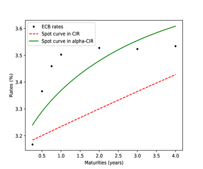
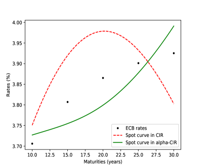
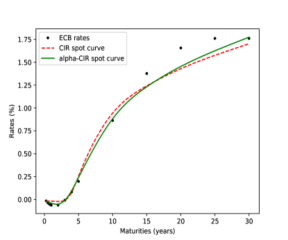
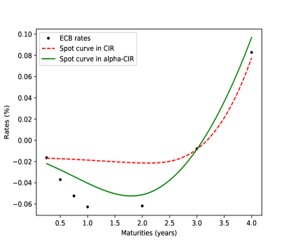
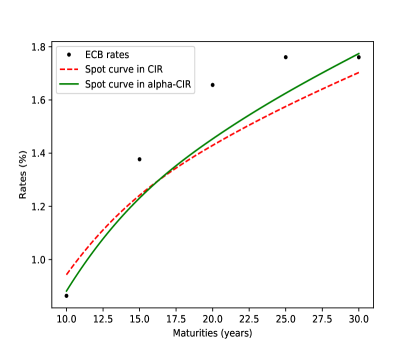
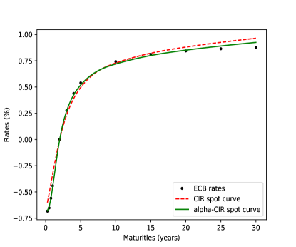
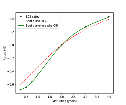
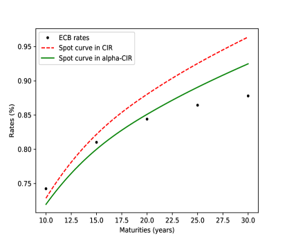
Parameters of models at dates with the best performance are presented in Tab. 2 and related plots in Fig.1, Fig.2 and Fig.3. The yield curves in the $\alpha$-CIR model turn out to be much more flexible than the CIR curves and almost all market quotes are better approached by the $\alpha$-CIR curve.

Date Model Parameters Error $\times 100$
$a$ $b$ $d_{1}$ $d_{2}$ $\alpha$
06.10.2010 CIR 0.011 0.000 0.002 2.352
$\alpha$-CIR 1.384 0.002 0.000 0.074 1.031 0.599
03.12.2014 CIR 1.332 0.000 0.032 177.865
$\alpha$-CIR 9.999 0.000 1.55 x $10^{-6}$ 0.752 1.057 56.485
08.04.2022 CIR -0.066 0.006 0.692 24.102
$\alpha$-CIR 0.939 0.005 1.902 9.12 x $10^{-6}$ 1.999 0.831
Table 2: Parameters of CIR and $\alpha$-CIR models for dates with the greatest error reduction.
Refer to caption
Refer to caption
Refer to caption
Figure 1: Calibration to the ECB rates from 6.10.2010. View for all/small/large maturities.
Refer to caption
Refer to caption
Refer to caption
Figure 2: Calibration to the ECB rates from 3.12.2014. View for all/small/large maturities.
Refer to caption
Refer to caption
Refer to caption
Figure 3: Calibration to the ECB rates from 8.04.2022. View for all/small/large maturities.

In our investigation we did not observe a significant error reduction by adding further stable noise components to the equation (4.12). Typical results we obtained in our implementation look like those in Tab.3, Tab.4 and Tab.5, where GCIR($k$) stands for the generalized CIR equation with $k$-dimensional noise. However, despite negligible calibration improvements, dimensions $k\geq 3$ may be desirable to adjust the heaviness of the tails of $R$. We observed that in the calibration process of GCIR($k$), $k\geq 3$, our algorithm was adding heavier noises than the one $\alpha$-stable noise appearing in the $\alpha$-CIR model.

Model Calibration error $\times 100$ Stability indices
CIR 2.35231805 $\alpha=2$
GCIR(1) 0.59992129 $\alpha_{1}=1.031$
GCIR(2) 0.5907987 $\alpha_{1}=1.02$, $\alpha_{2}=1.014$
GCIR(3) 0.58845355 $\alpha_{1}=1.017$, $\alpha_{2}=1.008$, $\alpha_{3}=1.007$
GCIR(4) 0.058819833 $\alpha_{1}=1.00944$, $\alpha_{2}=1.00943$, $\alpha_{3}=1.008$, $\alpha_{4}=1.006$
GCIR(5) 0.058796683 $\alpha_{1}=1.01$, $\alpha_{2}=1.009$, $\alpha_{3}=1.00898$, $\alpha_{4}=1.00896$, $\alpha_{5}=1.0003$
Table 3: Error reduction - calibration to the ECB rates from 6.10.2010.
Model Calibration error $\times 100$ Stability indices
CIR 177.86453440 $\alpha=2$
GCIR(1) 177.86453440 $\alpha=2$
GCIR(2) 56.48507979 $\alpha_{1}=2$, $\alpha_{2}=1.057$
GCIR(3) 56.44050315 $\alpha_{1}=2$, $\alpha_{2}=1.057$, $\alpha_{3}=1.056$
GCIR(4) 56.44050315 $\alpha_{1}=2$, $\alpha_{2}=1.602$, $\alpha_{3}=1.05728$, $\alpha_{4}=1.05724$
GCIR(5) 56.44050315 $\alpha_{1}=2$, $\alpha_{2}=1.611$, $\alpha_{3}=1.589$, $\alpha_{4}=1.05724$, $\alpha_{5}=1.05722$
Table 4: Error reduction - calibration to the ECB rates from 3.12.2014.
Model Calibration error $\times 100$ Stability indices
CIR 24.10280133 $\alpha=2$
GCIR(1) 24.10280133 $\alpha=2$
GCIR(2) 0.83059934 $\alpha_{1}=2$, $\alpha_{2}=1.99$
GCIR(3) 0.83055904 $\alpha_{1}=2$, $\alpha_{2}=1.17$, $\alpha_{3}=1.14$
GCIR(4) 0.83050323 $\alpha_{1}=2$, $\alpha_{2}=1.35$, $\alpha_{3}=1.25$, $\alpha_{4}=1.21$
GCIR(5) 0.83049801 $\alpha_{1}=2$, $\alpha_{2}=1.53$, $\alpha_{3}=1.48$, $\alpha_{4}=1.35$, $\alpha_{5}=1.23$
Table 5: Error reduction - calibration to the ECB rates from 8.04.2022.

4.2.2 Remarks on computational methodology

Our computations were implemented in the Python programming language. The calibration error was minimized with the use of the Nelder-Mead algorithm which turned out to be most effective among all available algorithms for local minimization in the Python library. The computation time of calibration for the $\alpha$-CIR model lied in most cases in the range 100-300 seconds. Calibration of models with a higher number of noise components took typically about 800 seconds but some outliers with 10.000 seconds also appeared. This stays in a strong contrast to the CIR model for which the closed form formulas shorten the calibration to the 2 second limit. We suspect that global optimization algorithms would provide even better fit, but they were too slow for the data with more than several maturities.

5 Appendix

5.1 Proof of Proposition 2.1

Proof: $(A)$ It was shown in [16, Theorem 5.3] that the generator of a general positive Markovian short rate generating an affine model is of the form

$\displaystyle\mathcal{A}f(x)=$ $\displaystyle cxf^{\prime\prime}(x)+(\beta x+\gamma)f^{\prime}(x)$ (5.1)
$\displaystyle+\int_{(0,+\infty)}\Big{(}f(x+y)-f(x)-f^{\prime}(x)(1\wedge y)\Big{)}(m(\textnormal{d}y)+x\mu(\textnormal{d}y)),\quad x\geq 0,$

for $f\in\mathcal{L}(\Lambda)\cup C_{c}^{2}(\mathbb{R}_{+})$, where $\mathcal{L}(\Lambda)$ is the linear hull of $\Lambda:=\{f_{\lambda}:=e^{-\lambda x},\lambda\in(0,+\infty)\}$ and $C_{c}^{2}(\mathbb{R}_{+})$ stands for the set of twice continuously differentiable functions with compact support in $[0,+\infty)$. Above $c,\gamma\geq 0$, $\beta\in\mathbb{R}$ and $m(\textnormal{d}y)$, $\mu(\textnormal{d}y)$ are nonnegative Borel measures on $(0,+\infty)$ satisfying

$$\displaystyle\int_{(0,+\infty)}(1\wedge y)m(\textnormal{d}y)+\int_{(0,+\infty)}(1\wedge y^{2})\mu(\textnormal{d}y)<+\infty.$$ (5.2)

The generator of the short rate process given by (2.1) equals

$\displaystyle\mathcal{A}_{R}f(x)=$ $\displaystyle f^{\prime}(x)F(x)+\frac{1}{2}f^{\prime\prime}(x)\langle QG(x),G(x)\rangle$
$\displaystyle+\int_{\mathbb{R}^{d}}\Big{(}f(x+\langle G(x),y\rangle)-f(x)-f^{\prime}(x)\langle G(x),y\rangle\Big{)}\nu(\textnormal{d}y)$
$\displaystyle=$ $\displaystyle f^{\prime}(x)F(x)+\frac{1}{2}f^{\prime\prime}(x)\langle QG(x),G(x)\rangle$
$\displaystyle+\int_{\mathbb{R}}\Big{(}f(x+v)-f(x)-f^{\prime}(x)v\Big{)}\nu_{G(x)}(\textnormal{d}v)$

where $f$ is a bounded, twice continuously differentiable function.

By Proposition 5.1 below, the support of the measure $\nu_{G(x)}$ is contained in $[-x,+\infty)$, thus it follows that

$\displaystyle\mathcal{A}_{R}f(x)=$ $\displaystyle f^{\prime}(x)F(x)+\frac{1}{2}f^{\prime\prime}(x)\langle QG(x),G(x)\rangle$
$\displaystyle+\int_{(0,+\infty)}\Big{(}f(x+v)-f(x)-f^{\prime}(x)(1\wedge v)\Big{)}\nu_{G(x)}(\textnormal{d}v)$
$\displaystyle+f^{\prime}(x)\int_{(0,+\infty)}\Big{(}(1\wedge v)-v\Big{)}\nu_{G(x)}(\textnormal{d}v)$
$\displaystyle+\int_{(-\infty,0)}\Big{(}f(x+v)-f(x)-f^{\prime}(x)v\Big{)}\nu_{G(x)}(\textnormal{d}v)$
$\displaystyle=$ $\displaystyle\frac{1}{2}f^{\prime\prime}(x)\langle QG(x),G(x)\rangle+f^{\prime}(x)\left[F(x)+\int_{(1,+\infty)}\Big{(}1-v\Big{)}\nu_{G(x)}(\textnormal{d}v)\right]$
$\displaystyle+\int_{(0,+\infty)}\Big{(}f(x+v)-f(x)-f^{\prime}(x)(1\wedge v)\Big{)}\nu_{G(x)}(\textnormal{d}v)$
$\displaystyle+\int_{[-x,0)}\Big{(}f(x+v)-f(x)-f^{\prime}(x)v\Big{)}\nu_{G(x)}(\textnormal{d}v).$ (5.3)

Comparing (5.1) with (5.1) applied to a function $f_{\lambda}$ with $\lambda>0$ such that $f_{\lambda}(x)=e^{-\lambda x}$ for $x\geq 0$, we get

$\displaystyle cx\lambda^{2}-(\beta x+\gamma)\lambda$
$\displaystyle+\int_{(0,+\infty)}\Big{(}e^{-\lambda y}-1+\lambda(1\wedge y)\Big{)}(m(\textnormal{d}y)+x\mu(\textnormal{d}y))$
$\displaystyle-\frac{1}{2}\lambda^{2}\langle QG(x),G(x)\rangle+\left[F(x)+\int_{(1,+\infty)}\Big{(}1-v\Big{)}\nu_{G(x)}(\textnormal{d}v)\right]\lambda$
$\displaystyle-\int_{(0,+\infty)}\Big{(}e^{-\lambda v}-1+\lambda(1\wedge v)\Big{)}\nu_{G(x)}(\textnormal{d}v)$
$\displaystyle=\int_{[-x,0)}\Big{(}e^{-\lambda v}-1+\lambda v\Big{)}\nu_{G(x)}(\textnormal{d}v),\quad\lambda>0,x\geq 0.$ (5.4)

Comparing the left and the right sides of (5.4) we see that the left side grows no faster than a quadratic polynomial of $\lambda$ while the right side grows faster that $de^{\lambda y}$ for some $d,y>0$, unless the support of the measure $\nu_{G(x)}(\textnormal{d}v)$ is contained in $[0,+\infty)$. It follows that $\nu_{G(x)}(\textnormal{d}v)$ is concentrated on $[0,+\infty)$, hence $(a)$ follows, and

$\displaystyle cx\lambda^{2}-(\beta x+\gamma)\lambda$
$\displaystyle-\frac{1}{2}\lambda^{2}\langle QG(x),G(x)\rangle+\left[F(x)+\int_{(1,+\infty)}\Big{(}1-v\Big{)}\nu_{G(x)}(\textnormal{d}v)\right]\lambda$
$\displaystyle=\int_{(0,+\infty)}\Big{(}e^{-\lambda y}-1+\lambda(1\wedge y)\Big{)}\left(\nu_{G(x)}(\textnormal{d}y)-m(\textnormal{d}y)-x\mu(\textnormal{d}y)\right),\quad\lambda>0,x\geq 0.$ (5.5)

Dividing both sides of the last equality by $\lambda^{2}$ and using the estimate

$$\frac{e^{-\lambda y}-1+\lambda(1\wedge y)}{\lambda^{2}}\leq\left(\frac{1}{2}y^{2}\right)\wedge\left(\frac{e^{-\lambda}-1+\lambda}{\lambda^{2}}\right)$$

we get that that the left side of (5.5) converges to $cx-\frac{1}{2}\langle QG(x),G(x)\rangle$ as $\lambda\rightarrow+\infty$, while the right side converges to 00. This yields (2.15), i.e.

$\displaystyle cx=$ $\displaystyle\frac{1}{2}\langle QG(x),G(x)\rangle,\quad x\geq 0.$ (5.6)

Next, fixing $x\geq 0$ and comparing (5.1) with (5.1) applied to a function from the domains of both generators and such that $f(x)=f^{\prime}(x)=f^{\prime\prime}(x)=0$ we get

$$\int_{(0,+\infty)}f(x+y)(m(\textnormal{d}y)+x\mu(\textnormal{d}y))=\int_{(0,+\infty)}f(x+v)\nu_{G(x)}(\textnormal{d}v)$$

for any such a function, which yields

$$\displaystyle\nu_{G(x)}(\textnormal{d}v)\mid_{(0,+\infty)}=m(\textnormal{d}v)+x\mu(\textnormal{d}v),\quad x\geq 0.$$ (5.7)

This implies also

$\displaystyle\beta x+\gamma=$ $\displaystyle F(x)+\int_{(1,+\infty)}\Big{(}1-v\Big{)}\nu_{G(x)}(\textnormal{d}v),\quad x\geq 0.$ (5.8)

$(b)$ Setting $x=0$ in (5.7) yields

$$\displaystyle\nu_{G(0)}(\textnormal{d}v)\mid_{(0,+\infty)}=m(\textnormal{d}v).$$ (5.9)

To prove (2.14), by (5.2) and (5.9), we need to show that

$$\displaystyle\int_{(1,+\infty)}v\nu_{G(0)}(\textnormal{d}v)<+\infty.$$ (5.10)

It is true if $G(0)=0$ and for $G(0)\neq 0$ the following estimate holds

$\displaystyle\int_{(1,+\infty)}v\nu_{G(0)}(\textnormal{d}v)$ $\displaystyle=\int_{\mathbb{R}^{d}}\langle G(0),y\rangle\mathbf{1}_{[1,+\infty)}(\langle G(0),y\rangle)\nu(\textnormal{d}y)$
$\displaystyle\leq\mid G(0)\mid\int_{\mathbb{R}^{d}}\mid y\mid\mathbf{1}_{[1/\mid G(0)\mid,+\infty)}(\mid y\mid)\nu(\textnormal{d}y),$

and (5.10) follows.

$(c)$ (2.16) follows from (5.7) and (5.9). To prove (2.17) we use (2.16), (2.14) and the following estimate for $x\geq 0$:

$\displaystyle\int_{0}^{+\infty}(v^{2}\wedge v)\nu_{G(x)}(\textnormal{d}v)$ $\displaystyle=\int_{\mathbb{R}^{d}}(\mid\langle G(x),y\rangle\mid^{2}\wedge\langle G(x),y\rangle)\nu(\textnormal{d}y)$
$\displaystyle\leq\Big{(}\mid G(x)\mid^{2}\vee\mid G(x)\mid\Big{)}\int_{\mathbb{R}^{d}}(\mid y\mid^{2}\wedge\mid y\mid)\nu(\textnormal{d}y)<+\infty.$

$(d)$ It follows from (5.8) and (2.16) that

$\displaystyle\beta x+\gamma$ $\displaystyle=F(x)+\int_{(1,+\infty)}(1-v)\nu_{G(x)}(\textnormal{d}v)$
$\displaystyle=F(x)+\int_{(1,+\infty)}(1-v)\nu_{G(0)}(\textnormal{d}v)+x\int_{(1,+\infty)}(1-v)\mu(\textnormal{d}v),\quad x\geq 0.$

Consequently, (2.18) follows with

$$a:=\Big{(}\beta-\int_{(1,+\infty)}(1-v)\mu(\textnormal{d}v)\Big{)},\ b:=\Big{(}\gamma-\int_{(1,+\infty)}(1-v)\nu_{G(0)}(\textnormal{d}v)\Big{)},$$

and $b\geq\int_{(1,+\infty)}(v-1)\nu_{G(0)}(\textnormal{d}v)$ because $\gamma\geq 0$.

$(B)$ We use (5.8), (2.18) and (5.7) to write (5.1) in the form

$\displaystyle\mathcal{A}f(x)=cxf^{\prime\prime}(x)$ $\displaystyle+\Big{[}ax+b+\int_{(1,+\infty)}(1-v)\nu_{G(x)}(\textnormal{d}v)\Big{]}f^{\prime}(x)$
$\displaystyle+\int_{(0,+\infty)}[f(x+v)-f(x)-f^{\prime}(x)(1\wedge v)]\nu_{G(x)}(\textnormal{d}v)\}.$

In view of (5.7) and (5.9) we see that (B) is true.

Proposition 5.1

Let $G:[0,+\infty)\rightarrow\mathbb{R}^{d}$ be continuous. If the equation (2.1) has a non-negative strong solution for any initial condition $R(0)=x\geq 0$, then

$$\displaystyle\forall x\geq 0\quad\nu{\{y\in\mathbb{R}^{d}:x+\langle G(x),y\rangle<0\}}=0.$$ (5.11)

In particular, the support of the measure $\nu_{G(x)}(\textnormal{d}v)$ is contained in $[-x,+\infty)$.

Proof: Let us assume to the contrary, that for some $x\geq 0$

$$\nu{\{y\in\mathbb{R}^{d}:x+\langle G(x),y\rangle<0\}}>0.$$

Then there exists $c>0$ such that

$$\nu{\{y\in\mathbb{R}^{d}:x+\langle G(x),y\rangle<-c\}}>0.$$

Let $A\subseteq\{y\in\mathbb{R}^{d}:x+\langle G(x),y\rangle<-c\}$ be a Borel set separated from zero. By the continuity of $G$ we have that for some $\varepsilon>0$:

$$\displaystyle\tilde{x}+\langle G(\tilde{x}),y\rangle<-\frac{c}{2},\quad\tilde{x}\in[(x-\varepsilon)\vee 0,x+\varepsilon],\quad y\in A.$$ (5.12)

Let $Z^{2}$ be a Lévy processes with characteristics $(0,0,\nu^{2}(dy))$, where $\nu^{2}(dy):=\mathbf{1}_{A}(y)\nu(dy)$ and $Z^{1}$ be defined by $Z(t)=Z^{1}(t)+Z^{2}(t)$. Then $Z^{1},Z^{2}$ are independent and $Z^{2}$ is a compound Poisson process. Let us consider the following equations

$$\displaystyle dR(t)=F(R(t))dt+\langle G(R(t-)),dZ(t)\rangle,\quad R(0)=x,$$
$$\displaystyle dR^{1}(t)=F(R^{1}(t))dt+\langle G(R^{1}(t-)),dZ^{1}(t)\rangle,\quad R^{1}(0)=x.$$

For the exit time $\tau_{1}$ of $R^{1}$ from the set $[(x-\varepsilon)\vee 0,x+\varepsilon]$ and the first jump time $\tau_{2}$ of $Z^{2}$ we can find $T>0$ such that $\mathbb{P}(\tau_{1}>T,\tau_{2}<T)=\mathbb{P}(\tau_{1}>T)\mathbb{P}(\tau_{2}<T)>0$. On the set $\{\tau_{1}>T,\tau_{2}<T\}$ we have $R(\tau_{2}-)=R^{1}(\tau_{2}-)$ and therefore

$$R(\tau_{2})=R^{1}(\tau_{2}-)+\langle G(R^{1}(\tau_{2}-)),\triangle Z^{2}(\tau_{2})\rangle<-\frac{c}{2}.$$

In the last inequality we used (5.12). This contradicts the positivity of $R$. $\square$

5.2 Proof of Theorem 3.11

Proof: In view of Theorem 3.1 the generating pairs $(G,Z)$ are such that

$$\displaystyle J_{1}(bG_{1}(x))+J_{2}(bG_{2}(x))=x\tilde{J}_{\mu}(b),\quad b,x\geq 0,$$ (5.13)

where $\tilde{J}_{\mu}$ takes the form (3.54) or (3.59). We deduce from (5.13) the form of $G$ and characterize the noise $Z$. First let us consider the case when

$$\displaystyle\left(\frac{G_{2}(x)}{G_{1}(x)}\right)^{\prime}=0,\qquad x>0.$$ (5.14)

Then $G(x)$ can be written in the form

$$\displaystyle G(x)=g(x)\cdot\left(\begin{array}[]{ccc}G_{1}\\ G_{2},\end{array}\right),\quad x\geq 0,$$

with some function $g(x)\geq 0,x\geq 0$, and constants $G_{1}>0,G_{2}>0$. Equation (2.1) amounts then to

$\displaystyle dR(t)$ $\displaystyle=F(R(t))+g(R(t-))\left(G_{1}dZ_{1}(t)+G_{2}dZ_{2}(t)\right)$
$\displaystyle=F(R(t))+g(R(t-))d\tilde{Z}(t),\quad t\geq 0,$

which is an equation driven by the one dimensional Lévy process $\tilde{Z}(t):=G_{1}Z_{1}(t)+G_{2}Z_{2}(t)$. It follows that $\tilde{Z}$ is $\alpha_{1}$-stable with $\alpha_{1}\in(1,2]$ and that $g(x)=c_{0}x^{1/\alpha_{1}},c_{0}>0$. Notice that $Z^{G(x)}(t)=c_{0}x^{\frac{1}{\alpha_{1}}}\tilde{Z}$, so $J_{Z^{G(x)}}(b)=c_{\alpha_{1}}(c_{0}x^{\frac{1}{\alpha_{1}}}b)^{\alpha_{1}}=xc_{0}^{\alpha_{1}}c_{\alpha_{1}}b^{\alpha_{1}}$ and $c_{0}=(\frac{\eta_{1}}{c^{\alpha_{1}}})^{\frac{1}{\alpha_{1}}}$. Hence (3.54) holds and this proves $(Ia)$.

If (5.14) is not satisfied, then

$$\displaystyle\left(\frac{G_{2}(x)}{G_{1}(x)}\right)^{\prime}\neq 0,\quad x\in(\underline{x},\bar{x}),$$ (5.15)

for some interval $(\underline{x},\bar{x})\subset(0,+\infty)$. In the rest of the proof we consider this case and prove $(Ib)$ and $(II)$.

$(Ib)$ From the equation

$$\displaystyle J_{1}(bG_{1}(x))+J_{2}(bG_{2}(x))=x\eta_{1}b^{\alpha_{1}},\quad b\geq 0,\ x\geq 0,$$ (5.16)

we explicitly determine unknown functions. Inserting $b/G_{1}(x)$ for $b$ yields

$$\displaystyle J_{1}(b)+J_{2}\left(b\frac{G_{2}(x)}{G_{1}(x)}\right)=\eta_{1}\frac{x}{G_{1}^{\alpha_{1}}(x)}b^{\alpha_{1}},\quad b\geq 0,\quad x>0.$$ (5.17)

Differentiation over $x$ yields

$$J_{2}^{\prime}\left(b\frac{G_{2}(x)}{G_{1}(x)}\right)\cdot b\left(\frac{G_{2}(x)}{G_{1}(x)}\right)^{\prime}=\eta_{1}\left(\frac{x}{G_{1}^{\alpha_{1}}(x)}\right)^{\prime}b^{\alpha_{1}},\quad b\geq 0,\quad x>0.$$

Using (5.15) and dividing by $\left(\frac{G_{2}(x)}{G_{1}(x)}\right)^{\prime}$ leads to

$$J_{2}^{\prime}\left(b\frac{G_{2}(x)}{G_{1}(x)}\right)\cdot b=\eta_{1}\frac{\left(\frac{x}{G^{\alpha_{1}}_{1}(x)}\right)^{\prime}}{\left(\frac{G_{2}(x)}{G_{1}(x)}\right)^{\prime}}\cdot b^{\alpha_{1}},\quad b\geq 0,\quad x\in(\underline{x},\bar{x}).$$

By inserting $b\frac{G_{1}(x)}{G_{2}(x)}$ for $b$ one computes the derivative of $J_{2}$:

$$J_{2}^{\prime}(b)=\eta_{1}\frac{\left(\frac{x}{G^{\alpha_{1}}_{1}(x)}\right)^{\prime}\left(\frac{G_{1}(x)}{G_{2}(x)}\right)^{\alpha_{1}-1}}{\left(\frac{G_{2}(x)}{G_{1}(x)}\right)^{\prime}}\cdot b^{\alpha_{1}-1},\quad b>0,\quad x\in(\underline{x},\bar{x}).$$

Fixing $x$ and integrating over $b$ provides

$$\displaystyle J_{2}(b)=c_{2}b^{\alpha_{1}},\quad b>0,$$ (5.18)

with some $c_{2}\geq 0$. Actually $c_{2}>0$ as $Z_{2}$ is of infinite variation and $J_{2}$ can not disappear.

By the symmetry of (5.16) the same conclusion holds for $J_{1}$, i.e.

$$\displaystyle J_{1}(b)=c_{1}b^{\alpha_{1}},\quad b>0,$$ (5.19)

with $c_{1}>0$. Using (5.18) and (5.19) in (5.16) gives us (3.58). This proves $(Ib)$.

$II)$ Solving the equation

$$\displaystyle J_{1}(bG_{1}(x))+J_{2}(bG_{2}(x))=x(\eta_{1}b^{\alpha_{1}}+\eta_{2}b^{\alpha_{2}}),\quad b,x\geq 0,$$ (5.20)

in the same way as we solved (5.16) yields that

$$\displaystyle J_{1}(b)=c_{1}b^{\alpha_{1}}+c_{2}b^{\alpha_{2}},\quad J_{2}(b)=d_{1}b^{\alpha_{1}}+d_{2}b^{\alpha_{2}},\quad b\geq 0,$$ (5.21)

with $c_{1},c_{2},d_{1},d_{2}\geq 0$, $c_{1}+c_{2}>0,d_{1}+d_{2}>0$. From (5.20) and (5.21) we can specify the following conditions for $G$:

$\displaystyle c_{1}G_{1}^{\alpha_{1}}(x)+d_{1}G_{2}^{\alpha_{1}}(x)$ $\displaystyle=\eta_{1}x,$ (5.22)
$\displaystyle c_{2}G_{1}^{\alpha_{2}}(x)+d_{2}G_{2}^{\alpha_{2}}(x)$ $\displaystyle=\eta_{2}x.$ (5.23)

We will show that $c_{1}>0,c_{2}=0,d_{1}=0,d_{2}>0$ by excluding the opposite cases.

If $c_{1}>0,c_{2}>0$, one computes from (5.22)-(5.23) that

$$\displaystyle G_{1}(x)=\left(\frac{1}{c_{1}}(\eta_{1}x-d_{1}G_{2}^{\alpha_{1}}(x))\right)^{\frac{1}{\alpha_{1}}}=\left(\frac{1}{c_{2}}(\eta_{2}x-d_{2}G_{2}^{\alpha_{2}}(x))\right)^{\frac{1}{\alpha_{2}}},\quad x\geq 0.$$ (5.24)

This means that, for each $x\geq 0$, the value $G_{2}(x)$ is a solution of the following equation of the $y$-variable

$$\displaystyle\left(\frac{1}{c_{1}}(\eta_{1}x-d_{1}y^{\alpha_{1}})\right)^{\frac{1}{\alpha_{1}}}=\left(\frac{1}{c_{2}}(\eta_{2}x-d_{2}y^{\alpha_{2}})\right)^{\frac{1}{\alpha_{2}}},$$ (5.25)

with $y\in\left[0,\left(\frac{\gamma_{1}x}{d_{1}}\right)^{\frac{1}{\alpha_{1}}}\wedge\left(\frac{\gamma_{2}x}{d_{2}}\right)^{\frac{1}{\alpha_{2}}}\right]$. If $d_{1}=0$ or $d_{2}=0$ we compute $y=y(x)$ from (5.25) and see that $d_{1}y^{\alpha_{1}}$ or $d_{2}y^{\alpha_{2}}$ must be negative either for $x$ sufficiently close to 00 or $x$ sufficiently large. Now we need to exclude the case $d_{1}>0,d_{2}>0$. However, in the case $c_{1},c_{2},d_{1},d_{2}>0$ equation (5.25) has no solutions because, for sufficiently large $x>0$, the left side of (5.25) is strictly less than the right side. This inequality follows from Proposition 5.2 proven below.

So, we proved that $c_{1}\cdot c_{2}=0$ and similarly one proves that $d_{1}\cdot d_{2}=0$. The case $c_{1}=0,c_{2}>0,d_{1}>0,d_{2}=0$ can be rejected because then $J_{1}$ would vary regularly with index $\alpha_{2}$ and $J_{2}$ with index $\alpha_{1}$, which is a contradiction. It follows that $c_{1}>0,c_{2}=0,d_{1}=0,d_{2}>0$ and in this case we obtain (3.60) from (5.22) and (5.23). $\square$

Proposition 5.2

Let $a,b,c,d>0$, $\gamma\in(0,1)$, $2\geq\alpha_{1}>\alpha_{2}>1$. Then for sufficiently large $x>0$ the following inequalities are true

$$\displaystyle\Big{(}ax-(bx-cz)^{\gamma}\Big{)}^{\frac{1}{\gamma}}-dz>0,\qquad z\in\Big{[}0,\frac{b}{c}x\Big{]},$$ (5.26)
$$\displaystyle(bx-cy^{\alpha_{1}})^{\frac{1}{\alpha_{1}}}<(ax-dy^{\alpha_{2}})^{\frac{1}{\alpha_{2}}},\quad y\in\Big{[}0,\Big{(}\frac{b}{c}x\Big{)}^{\frac{1}{\alpha_{1}}}\wedge\Big{(}\frac{a}{d}x\Big{)}^{\frac{1}{\alpha_{2}}}\Big{]}.$$ (5.27)

Proof: First we prove (5.26) and write it in the equivalent form

$$\displaystyle ax\geq(dz)^{\gamma}+(bx-cz)^{\gamma}=:h(z).$$ (5.28)

Since

$$h^{\prime}(z)=\gamma\Big{(}d^{\gamma}z^{\gamma-1}-c(bx-cz)^{\gamma-1}\Big{)},$$
$$h^{\prime\prime}(z)=\gamma(\gamma-1)\Big{(}d^{\gamma}z^{\gamma-2}+c^{2}(bx-cz)^{\gamma-2}\Big{)}<0,\quad z\in\Big{[}0,\frac{b}{c}x\Big{]},$$

the function $h$ is concave and attains its maximum at point

$$z_{0}:=\theta x:=\frac{bc^{\frac{1}{\gamma-1}}}{d^{\frac{\gamma}{\gamma-1}}+c^{\frac{\gamma}{\gamma-1}}}x\in\Big{[}0,\frac{b}{c}x\Big{]},$$

which is a root of $h^{\prime}$. It follows that

$\displaystyle h(z)\leq h(\theta x)$ $\displaystyle=(\theta x)^{\gamma}+(bx-c\theta x)^{\gamma}$
$\displaystyle=(\theta^{\gamma}+(b-c\theta)^{\gamma})x^{\gamma}<ax,$

provided that $x$ is sufficiently large and (5.26) follows. (5.27) follows from (5.26) by setting $\gamma=\alpha_{2}/\alpha_{1}$, $z=y^{\alpha_{1}}$. $\square$

References

  • [1] Alfonsi A.: Affine Diffusions and Related Processes: Simulation, Theory and Applications, (2015), Springer,
  • [2] Barndorff-Nielsen O.E., Shephard N.: Modelling by Lévy processes for financial econometrics, (2001), In: Barndorff-Nielsen, O.E., et al. (eds.) Lévy Processes: Theory and Applications, 283 - 318. Birkhäuser,
  • [3] Barski M., Zabczyk J.: On CIR equations with general factors, (2020), SIAM J.Financial Mathematics, 11,1,131-147,
  • [4] Barski M., Zabczyk J.: Bond Markets with Lévy Factors, (2020), Cambridge University Press,
  • [5] Barski M., Zabczyk J.: A note on generalized CIR equations, (2021), Communications in Information and Systems, 21, 2, 209-218,
  • [6] Cheridito P., Filipović D., Kimmel R.L.: A note on the Dai - Singleton canonical representation of Affine Term Structure Models, (2010), Mathematical Finance , 20, 3, 509-519,
  • [7] Cox, I., Ingersoll, J., Ross, S.: A theory of the Term Structure of Interest Rates, (1985), Econometrica, 53, 385-408,
  • [8] Cuchiero C., Filipović D., Teichmann J.: Affine models, (2010), Encyclopedia of Quantitative Finance,
  • [9] Cuchiero C., Teichmann J.: Path properties and regularity of affine processes on general state spaces, (2013), Séminaire de Probabilités XLV,
  • [10] Dai Q., Singleton K.: Specification Analysis of Affine Term Structure Models, (2000), The Journal of Finance, 5, 1943-1978,
  • [11] Dawson D. A., Li Z.: Skew Convolution Semigroups and Affine Markov Processes, (2006), The Annals of Probability, 34(3), 1103-1142,
  • [12] Dawson D. A., Li Z.: Stochastic Equations, Flows and Measure-Valued Processes, (2012), The Annals of Probability, 40(2), 813-857,
  • [13] Duffie D., Filipović D., Schachermayer W.: Affine processes and applications in finance, (2003), The Annals of Applied Probability, 13(3), 984-1053,
  • [14] Duffie, D., Gârleanu, N.: Risk and valuation of collateralized debt obligations, (2001), Financial Analysts Journal, 57, 41-59,
  • [15] Bingham N. H., Goldie C. M., Teugels J. L.: Regular variation, Cambridge University Press (1989),
  • [16] Filipović, D.: A general characterization of one factor affine term structure models, (2001), Finance and Stochastics, 5, 389-412,
  • [17] Fu Z., Li Z.: Stochastic equations of non-negative processes with jumps, (2010), Stochastic Processes and their Applications, 120, 306-330,
  • [18] Hult H., Lindskog F.: Extremal Behavior of Stochastic Integrals Driven by Regularly Varying Lévy Processes, (2007), The Annals of Probability, 35(1), 309-339,
  • [19] Jiao Y., Ma C., Scotti S.: Alpha-CIR model with branching processes in sovereign interest rate modeling, (2017) Finance and Stochastics, 21, 789-813,
  • [20] Kawazu K., Watanabe S.: Branching processes with immigration and related limit theorems, (1971) Theory Probab. Appl., 16, 36-54,
  • [21] Keller-Ressel M., Mijatović A.: On the limit distributions of continuous-state branching processes with immigration , (2012) Stochastic Processes and their Applications, 122, 2329-2345,
  • [22] Keller-Ressel M., Steiner T.: Yield curve shapes and the asymptotic short rate distribution in affine one-factor models, (2008) Finance and Stochastics, 12, 149-172,
  • [23] Kyprianou, A.E.: Introductory Lectures on Fluctuations of Lévy Processes with Applications, Springer (2006),
  • [24] Li Z.: Measure-Valued Branching Markov Processes, Springer (2011),
  • [25] Li Z., Ma Ch.: Asymptotic properties of estimators in a stable Cox-Ingersoll-Ross model, (2015), Stochastic Processes and their Applications, 125, 3196-3233,
  • [26] Pinsky M.: Limit theorems for continuous state branching processes with immigration, (1972) Bulletin of the AMS 78(2), 242–244,
  • [27] Samorodnitsky G., Taqqu M.: Stable Non-Gaussian Random Processes, Chapman & Hall (1994),
  • [28] Sato, K.I.: Lévy Processes and Infinite Divisible Distributions, Cambridge University Press (1999),
  • [29] Vasiček, O.: An equilibrium characterization of the term structure, (1997), Journal of Financial Economics, 5, (2), 177-188.