Expansion of higher-dimensional cubical complexes
with application to quantum locally testable codes

Abstract

We introduce a higher-dimensional “cubical” chain complex and apply it to the design of quantum locally testable codes. Our cubical chain complex can be constructed for any dimension $t$, and in a precise sense generalizes the Sipser-Spielman construction of expander codes (case $t=1$) and the constructions by Dinur et. al and Panteleev and Kalachev of a square complex (case $t$=2), which have been applied to the design of classical locally testable and quantum low-density parity check codes respectively. For $t=4$ our construction gives a family of quantum locally testable codes conditional on a conjecture about robustness of four-tuples of random linear maps. These codes have linear dimension, inverse poly-logarithmic relative distance and soundness, and polylogarithmic-size parity checks.

Our complex can be built in a modular way from two ingredients. Firstly, the geometry (edges, faces, cubes, etc.) is provided by a set $G$ of size $N$, together with pairwise commuting sets of actions $A_{1},\ldots,A_{t}$ on it.

Secondly, the chain complex itself is obtained by associating local coefficient spaces, which are finite-dimensional vector spaces, with each geometric object, and introducing local maps on those coefficient spaces.

These maps are constructed from a family of local codes, each specified by a parity check matrix $h_{1},\ldots,h_{t}$.

We prove lower bounds on the expansion properties of this high-dimensional complex. Concretely, we show that, under the right assumption about the sets $A_{j}$, and about the codes $h_{j}$, at each level $i=1,\ldots,t-1$, the cycle and co-cycle expansion of the chain complex are linear in the dimension of the space of $i$-chains $C_{i}$, up to a multiplicative factor that is inverse polynomial in $n$, the size of the sets $A_{j}$. The assumptions we need are two-fold: firstly, each Cayley graph $\mathrm{Cay}(G,A_{j})$ needs to be a good (spectral) expander, and secondly, the families $(h_{1},\ldots,h_{t})$ and $(h_{1}^{\perp},\ldots,h_{t}^{\perp})$ both need to satisfy a form of robustness (that generalizes the condition of agreement testability for pairs of codes). While the first assumption is easy to satisfy, it is currently not known if the second can be achieved.

1 Introduction

Expander graphs are bounded-degree graphs with strong connectivity, or more precisely expansion, properties. Explicit constructions of expander graphs are non-trivial, but, by now, abound; their use is ubiquitous in algorithms design, complexity theory, combinatorics, and other areas. High-dimensional expanders generalize the expansion requirements of expander graphs to higher-dimensional structures, composed of vertices and edges as well as higher-dimensional faces. Constructions of high-dimensional expanders (HDX) are difficult and comparatively few techniques are known. In recent years HDX have found impactful applications to randomized algorithms, complexity theory, and the design of error-correcting codes, among others. In addition to their intrinsic interest as combinatorial/geometric objects, the increasing range of applications further motivates the study of HDX.

In this paper we introduce a natural generalization of a family of two-dimensional (graphs are one-dimensional) expanders introduced recently and independently in [DEL⁺22, PK22] and used to simultaneously construct the first good classical locally testable codes (LTC) [DEL⁺22, PK22] and the first qood quantum low-density parity check codes (qLDPC) [PK22]. We extend this construction to arbitrary dimensions and prove lower bounds on its cyclic and co-cyclic expansion, which we define below. The bounds that we obtain depend on underlying parameters of the complex, namely the (spectral) expansion of an associated family of Cayley graphs and a certain robustness-like property of an associated family of constant-sized local codes. The main application of our construction, which has been our primary motivation, is towards the construction of good quantum locally testable codes (qLTC). We make progress towards this goal with two caveats. First, our construction loses polylogarithmic factors, so the parameters are “almost” good. Second, we require an unproven conjecture regarding the existence of good polylog-size local codes, akin to that conjectured in [KP22].

1.1 Construction

For any integer $t\geqslant 1$ we construct a $t$-dimensional cubical chain complex that generalizes the Sipser-Spielman construction of expander codes [SS96] (case $t=1$) and the lifted product codes from [PK21] (case $t=2$) to higher dimensions $t\geqslant 3$.

The construction is based on two ingredients. Firstly, there is the cubical complex $X$, which is a purely geometric structure (technically, a graded incidence poset with certain good expansion properties). Secondly, there is a system of local coefficients (a sheaf $\mathcal{F}$, in the terminology of [FK22]) that is constructed from a family of classical codes of small (constant, or polylogarithmic in the size of the complex) dimension and good “robustness” properties. The chain complex is a sequence of coboundary maps from $i$-cochains to $i+1$-cochains,

$$C^{0}(X,\mathcal{F})\to C^{1}(X,\mathcal{F})\to\cdots\to C^{t}(X,\mathcal{F}).$$

We expand on these ingredients below.

We first describe the (higher-dimensional) cubical complex $X$. This complex can be constructed from any set $G$ of size $N=|G|$, and finite subsets of permutations $A_{1},\ldots,A_{t}$ of $G$ of size $n=|A_{i}|$. The sets $A_{i}$ should be closed under inverse and such that permutations taken from different sets commute. For example, in the $t=2$-dimensional case we can take $G$ to be any finite group and let $A_{1}$ act by multiplication on the left, and $A_{2}$ by multiplication on the right; this choice underlies the square complex from [DEL⁺22, PK22]. For larger $t\geqslant 3$, one can take $G$ an Abelian group, such as $G=\mathbb{Z}_{2}^{\log N}$, and let $A_{i}$ be subsets of generators of $G$ acting by multiplication on it. This choice has disadvantages (achieving the right expansion requires sets $A_{i}$ of size $\Omega(\log|G|)$) and other, more structured choices may be possible. The resulting complex $X(G;\{A_{i}\}_{i=1}^{t}$) is $2^{t}$-partite, with vertex set $G\times\{0,1\}^{t}$ and $k$-dimensional faces associated with the $2^{|S|}$ vertices $\{g\cdot\prod_{j\in T}a_{j}:\,T\subseteq S\}$, where $S\subseteq\{1,\ldots,t\}$ has size $|S|=k$ and $a_{j}\in A_{j}$. Edges coming from permutations in $A_{i}$ are said to have direction $i$, and more generally, a face has type $S$ if $S$ is the set of directions of edges it contains. See Section 3.1 for a complete description, and Figure 1 for an illustration.

The only requirement on the permutation sets $A_{i}$ is that the associated graphs $\mathrm{Cay}(G,A_{i})$, with vertex set $G$ and edge set $\{g,\pi(g)\}$ for $\pi\in A_{i}$, have good spectral expansion. As we will show, this suffices to imply expansion of a natural set of high-dimensional random walks on the cubical complex that are used in the proof of (co)-cycle expansion.

Next we describe the second main ingredient, which is the system of local coefficients, namely the sheaf structure over the geometrical complex $X$. To each face $f$ of the complex, which can be a vertex, an edge, a square, a cube, etc., we associate a small coefficient space that is in some sense dual to it. For example, suppose $t=3$ and our complex $X$ is a cubical complex. Fix a $1$-dimensional face, namely an edge. Its space of coefficients is a space of $2$-dimensional matrices. If the edge is labeled by direction $1$, then the matrix dimensions are labeled using the other directions of the complex, namely $2,3$. These spaces are described in detail in Section 3.2. We introduce a system of linear maps $\mathcal{F}_{f\to f^{\prime}}$ from the coefficient space of a $k$-face $f$ to that of a ($k+1$)-face $f^{\prime}$. These maps will be constructed from a collection of parity check matrices $h_{1},\ldots,h_{t}$, where each $h_{i}\in\mathbb{F}_{2}^{m_{i}\times n}$ for some $m_{i}\leqslant n$. These matrices will be used as follows. Suppose for example that, as before, $t=3$, $f$ is an edge and $f^{\prime}$ is a face that contains the edge $f$, as well as another (pair of) edges in direction $2$ (and a fourth edge, parallel to $f$). Then the map $\mathcal{F}_{f\to f^{\prime}}$ is obtained by taking the coefficient $x(f)\in\mathbb{F}_{2}^{m_{2}\times m_{3}}$ associated with $f$, expanding it in the second direction by applying $h_{2}^{T}$ to obtain $h_{2}^{T}x(f)\in\mathbb{F}_{2}^{n\times m_{3}}$, and then restricting to the row indexed by the face $f^{\prime}$ (which is uniquely identified by its edge in direction $2$, labeled by an element of $A_{2}$ which has size $n$) and returning the resulting row vector, an element of the coefficient space $\mathbb{F}_{2}^{m_{3}}$ associated with the face $f^{\prime}$. These maps are described in much more detail in Section 3.3 (where they are denoted $\textrm{co-res}_{f,f^{\prime}}$).

1.2 Two-way robustness

The main requirement on the parity check matrices $(h_{1},\ldots,h_{t})$ is that they are (jointly) two-way robust. A collection of linear transformations $h_{i}:\mathbb{F}_{2}^{n}\to\mathbb{F}_{2}^{k_{i}}$, $1\leqslant i\leqslant t$, is said to be two-way robust if the $t$-fold homological product of $h_{1}^{T},\ldots,h_{t}^{T}$ is coboundary expanding, and the same holds also for $(h_{1}^{\perp})^{T},\ldots,(h_{t}^{\perp})^{T}$, where for each $i$, $h_{i}^{\perp}:\mathbb{F}_{2}^{n}\to\mathbb{F}_{2}^{n-k_{i}}$ is (some) matrix that satisfies $h_{i}^{\perp}h_{i}^{T}=0$, i.e. the code with parity check matrix $h_{i}^{\perp}$ is dual to the code with parity check matrix $h_{i}$. We refer to Section 4.2 for the precise definition. The reason for considering the $t$-fold homological product is that this is precisely the local view of the complex from a vertex. Namely, the view when restricting to cells that contain a fixed vertex. So our requirements for global co-cycle expansion boils down to a local condition (two-way robustness) on the restriction of the code to cells around a vertex and a global condition (spectral expansion of each $\mathrm{Cay}(G,A_{i})$). This is in perfect analogy to previous works on co-cycle expansion of simplicial complexes [KKL14, EK16] and of cubical complexes [DEL⁺22, PK22].

The notion of two-way robustness is a direct generalization of the notion of product expansion from [PK22]. It implies in particular that all $h_{i},h_{i}^{\perp}$ have good distance as error correcting codes, and that for every $i\neq j$ the pair is agreement testable. For $t=2$ agreement testability is equivalent to product expansion which is equivalent to two-way robustness. However, for $t\geqslant 3$ these notions diverge, as studied in [Kal23]. In their breakthrough work constructing good quantum LDPC codes [PK22], Panteleev and Kalachev proved that a pair of random maps $h_{1},h_{2}$ satisfy, with high probability, a version of two-way robustness. The robustness parameters were later improved in [KP22, DHLV23], but only for a pair of random maps, namely $t=2$. For three or more maps it was conjectured in [KP22] that random maps are product expanding. We conjecture further that with high probability, a random collection of $t$ linear maps are two-way robust, see Conjecture 4.10. The conjecture in [KP22] addresses coboundary expansion only in level $t-1$, whereas we require coboundary expansion for all levels.

1.3 Main result on expansion

To state our main result we need to define the notions of distance and expansion that we consider. We will use the term systolic (resp. co-systolic) distance to denote the lowest weight of a $k$-cycle (co-cycle) that is not a $k$-boundary (co-boundary). Namely, if $C(X)$ is a chain complex with boundary map $\partial$ and coboundary map $\delta$, then

$$\mu_{\mathrm{syst}}(k)\,=\,\min\big{\{}|x|\,:\,x\in\ker\partial_{k}-\mathrm{im}\,\partial_{k+1}\big{\}},\qquad\mu_{\mathrm{cosyst}}(k)\,=\,\min\big{\{}|x|\,:\,x\in\ker\delta_{k}-\mathrm{im}\,\delta_{k-1}\big{\}}\;.$$

Here we employ the usual notation $\partial_{k}:C_{k}(X)\to C_{k-1}(X)$ and $\delta_{k}:C^{k}(X)\to C^{k+1}(X)$, with $C_{k}(X)$ and $C^{k}(X)$ the (isomorphic) spaces of chains and co-chains respectively.

We establish lower bounds on the systolic and co-systolic distance of the complex, as well as lower bounds on the cycle and co-cycle expansion, which we define next. The lower bounds are attained via bounding a locally-minimal version of distance (see Definition 2.2), using the strategy initiated in [KKL14, EK16], and used also in [PK22, DEL⁺22]. The cycle expansion of the complex is the smallest size of the boundary of a $k$-chain, relative to the distance of the $k$-chain to the set of $k$-cycles. More formally,

$$\varepsilon_{\mathrm{cyc}}(k)\,=\,\min\Big{\{}\frac{|\partial_{k}(x)|}{dist(x,\ker\partial_{k})}\,:\,x\in C_{k}(X)-\ker\partial_{k}\Big{\}}\;,$$

and similarly, co-cycle expansion is defined by

$$\varepsilon_{\mathrm{cocyc}}(k)\,=\,\min\Big{\{}\frac{|\delta_{k}(x)|}{dist(x,\ker\delta_{k})}\,:\,x\in C_{k}(X)-\ker\delta_{k}\Big{\}}\;.$$

In the definitions above, $dist(\cdot,\cdot)$ and $|\cdot|$ refers to the Hamming weight, or, in the case of a sheaf complex, the block-Hamming weight. For precise definitions of all these notions, we refer to Section 2.1. We remark that co-cycle expansion was first studied in [KKL14] in the simplicial setting. The term cosystolic expansion was introduced in [EK16], and combined both co-systolic distance and co-cycle expansion. In retrospect it makes sense to separate into two definitions as above.

Our main result can informally be stated as follows.

Theorem 1.1 (Main result on expansion, informal).

Let $G$ and $\{A_{i}\}$ be a set and collections of permutations on it such that the graphs $\mathrm{Cay}(G,A_{i})$ are each $\lambda$-expanding (see Definition 5.4). Let $N=|G|$ and $n=|A_{1}|=\cdots=|A_{t}|$. Let $(h_{1},\ldots,h_{t})$ be a collection of matrices $h_{j}\in\mathbb{F}_{2}^{m_{j}\times n}$ such that the family $(h_{1},\ldots,h_{t})$ is two-way $\kappa$-robust (see Definition 4.9). Assume that $\lambda$ is small enough compared to $\kappa$. Then the dimension-$t$ cubical chain complex constructed from $G,\{A_{i}\}$ and $\{h_{i}\}$ as in Definition 3.3 has the following properties.

1. For every $0\leqslant k\leqslant t-2$, the co-complex $C$ has $\mu_{\mathrm{cosyst}}(k)$ co-systolic distance, and has $\varepsilon_{\mathrm{cocyc}}(k)$ co-cycle expansion in dimension $k$ with $\mu_{\mathrm{cosyst}}(k)=\operatorname{poly}(\kappa,1/n)|X(k)|$ and $\varepsilon_{\mathrm{cocyc}}(k)=\operatorname{poly}(\kappa,1/n)$. Furthermore, for $k=t-1$ the co-complex $C$ has co-systolic distance in dimension $k$ with $\mu_{\mathrm{cosyst}}(k)=\operatorname{poly}(\kappa,1/n)|X(k)|$.

2. For every $2\leqslant k\leqslant t$, the complex $C$ has $\mu_{\mathrm{syst}}(k)$ systolic distance in dimension $k$, and has $\varepsilon_{\mathrm{cyc}}(k)$ cycle-expansion, with $\mu_{\mathrm{syst}}(k)=\operatorname{poly}(\kappa,1/n)|X(k)|$ and $\varepsilon_{\mathrm{cyc}}(k)=\operatorname{poly}(\kappa,1/n)$. Furthermore, for $k=1$ the complex $C$ has systolic distance in dimension $k$ with $\mu_{\mathrm{syst}}(k)=\operatorname{poly}(\kappa,1/n)|X(k)|$.

In the theorem, the polynomials implicit in the terms $\operatorname{poly}(\kappa,1/n)$ have a degree that may depend on $t$, so our bounds get exponentially worse as $t$ increases. The precise requirement on $\lambda$ also depends exponentially on $t$, i.e. the requirement is that $\lambda<\kappa^{t}\exp(-O(t^{2}))$. The main application we have in mind, to quantum locally testable codes, requires only $t=4$, and we did not attempt to optimize the dependence on $t$. We refer to Theorem 3.6 for a precise statement of the theorem.

We note that for $t=1$ and $n$ a constant, our theorem recovers the special case that Sipser-Spielman codes based on good enough expander graphs and good local codes have a linear distance. For $t=2$ and $n$ a constant, the theorem recovers the expansion properties of square complexes that underlie the constructions of locally testable and quantum low-density parity check codes from [DEL⁺22, PK22].

1.4 Towards quantum locally testable codes

The existence of good quantum error-correcting codes is one of the pillars that underlie the promise of quantum computing to deliver impactful applications in the long term. Good codes with low-density parity checks are particularly sought after for their potential application to fault-tolerance [Got14] and quantum complexity theory [ABN23]. In the past few years a flurry of works obtained better understanding and better parameters [EKZ22, HHO21, BE21, PK21] culminating in a construction of good quantum LDPC codes [PK22]. This was followed by a couple of related variants [LH22, LZ22, DHLV23]. These constructions rely on a well-known connection between the design of quantum codes and chain complexes. In particular, all existing constructions of good qLDPC rely on virtually the same length-$3$ chain complex, the “square complex” from [DEL⁺22] (which is also a special case of “balanced product codes” from [BE21] and of “lifted product codes” from [PK21]).

Quantum locally testable (qLTC) codes were introduced in [AE15] as a natural quantization of the notion of local testability for classical codes. Although the formal definition, first given in [EH17], is somewhat technical, quantum LTCs have the same intuitive basis as their classical counterparts — informally, whenever a word (quantum state) is at a certain relative distance $\delta$ from the codespace, this word must violate a fraction $\rho\,\delta$, for some constant $\rho>0$ referred to as the soundness of the LTC, of the parity checks. The first constructions of qLTCs with soundness that scales better than inverse polynomial were given in [Has17, LLZ22]. These achieve soundness $1/\log^{2}(n)$ and $1/\log(n)$ respectively; however, the distance of the code is small ($\Theta(\sqrt{n})$), the codes have constant dimension, and the weight of the parity checks is logarithmic.

Good quantum LTCs, with constant, or even sub-inverse-polylogarithmic, relative dimension, distance and soundness, are not known to exist. Such codes are expected to have applications in quantum complexity theory. Until recently the most prominent was the famous “NLTS conjecture” [EH17]. However, the NLTS theorem was recently proven without the use of qLTC [ABN23], relying only on the recent qLDPC constructions from [PK22, LZ22]).

While there is no formal connection with the long-standing quantum PCP conjecture [AAV13], it is natural to hope that progress on the former may eventually lead to progress on the latter. One reason is that LTCs are strongly tied to PCPs in the classical world, which, perhaps more philosophically, is due to the inherent local-to-global nature of both questions, where a global property (being a codeword in the case of LTC and being a minimum energy state in the case of qPCP) is to be tested by random local tests. The local to global aspect manifests in high dimensional expanders, shedding some insight as to the connection between these objects.

Our construction of higher-dimensional cubical complexes provides a template for qLTC with simultaneously non-trivial dimension, distance and soundness. For the sake of concreteness we describe this application in the special case where $N$ is a power of $2$ and $G$ is the Abelian group $G=\mathbb{Z}_{2}^{\log N}$. For a more general statement we refer to Corollary 3.7. Let $n=\lceil c\log N\rceil$, for a sufficiently large constant $c$ such that there exist sets $A_{1},\ldots,A_{4}$ of size $n=|A_{j}|$ such that the graphs $\mathrm{Cay}(G,A_{j})$ have spectral expansion at most $\lambda$, where $\lambda$ is sufficiently small compared to the robustness parameter $\kappa$. In particular, if $\kappa$ is a constant independent of $n$ then we can always make $\lambda$ small enough by increasing $c$, independently of $n$. This is because it is well-known that for any target $\lambda$ (possibly depending on $\kappa$) there is a constant $c(\lambda)=O(1/\lambda^{2})$ and subsets $A_{j}$ of $G$ of size $|A_{j}|=c(\lambda)\log|G|$ such that $\mathrm{Cay}(G,A_{j})$ is $\lambda$-expanding. (This can be shown by a probabilistic argument [AR94], and also by explicit constructions [AGHP92].)

With these choices we obtain the main corollary.

Corollary 1.2.

Assume the existence of two-way $\kappa$-robust $4$-tuples of codes, with constant robustness $\kappa>0$. Then there exists a CSS code $\mathcal{C}=CSS(H_{X},H_{Z})$ such that $\mathcal{C}$ is an $[\ell,k,d]$ quantum code with $\ell=\Omega(N\operatorname{poly}\log N)$, parity checks of weight $O(\log\ell)$, $k=\Omega(\ell)$ and $d=\Omega(\ell/\operatorname{poly}\log\ell)$. Furthermore, the code is qLTC with soundness $\rho\geqslant 1/\operatorname{poly}\log\ell$.

The result in Corollary 1.2 comes short of constructing good quantum LTC in two respects. Firstly, it requires an unproven conjecture on two-way robustness; and secondly, the parameters differ from ideal parameters by an inverse poly-logarithmic factor. Still, these parameters mark an exponential improvement compared to previously known qLTCs, narrowing the gap to the optimal qLTC. Overcoming both limitations will require further work. At present it is only known how to satisfy the assumption on robustness for pairs of matrices $(h_{1},h_{2})$, and even then only through a probabilistic existence argument, see [DHLV23, KP22]. However, families that are $1$-sided robust exist and can be constructed from e.g. smooth codes as in [DSW06, BV08] or possibly from Reed-Muller codes. Thus, even though we are unable to show their existence we can naturally expect that general families $(h_{1},\ldots,h_{t})$ exist that are two-way robust. Removing the poly-logarithmic factors may require further ideas. Nevertheless, by applying distance balancing, weight reduction, and soundness amplification techniques [WLH23a, WLH23b], one can achieve codes with constant rate, constant relative distance, constant soundness, but polylog locality; or codes with constant locality, but inverse polylog rate, inverse polylog relative distance, and inverse polylog soundness.

The codes from the theorem are explicit CSS codes, and in particular have an efficient encoder. Moreover, although we do not show this explicitly, we expect these codes to have linear-time decoders and noisy syndrome decoders (often referred to as single-shot decoders), along the same lines as [DHLV23, GTC⁺23]. Although there is no formal connection known, we observe that qLTC may be of additional relevance to the problem of noisy syndrome decoding. This is because a simpler problem than decoding from a noisy syndrome is deciding, given an approximate bound on the size of the syndrome, if the state is close to the codespace or not—which is precisely the problem solved by qLTCs. This observation suggests that, beyond the basic LDPC requirement, the LTC condition may have applications to e.g. fault-tolerance that have not yet been fully explored.

1.5 Proof idea

Our construction of a higher-dimensional cubical chain complex, when instantiated at $t=2$, is not identical to the chain complex of [PK22], but rather can be seen as a “$90^{\circ}$ rotation” of it as in [DHLV23]. The vector spaces participating in the chain complex are ordered by geometric dimension, a feature that facilitates generalization to $t>2$. The price is that our construction is not self-dual, in the sense that the geometric properties of the complex are different from those of the co-complex. Therefore, the argument for showing co-cycle expansion is different from the argument for showing cycle expansion. Nevertheless, the latter is based on a reduction to the former for a different co-complex that is, in some sense, dual to the original one.

We first explain the argument for co-cycle expansion. The co-systolic distance and the co-cycle expansion are both bounded as a consequence of a lower bound on the locally co-minimal distance of the co-complex, at each level $k\in\{0,\ldots,t-1\}$. The locally co-minimal distance is defined as the minimal weight of any co-cycle that is “locally minimal”, i.e. its weight cannot be reduced by adding the boundary of a local element (i.e. that is supported on a single link). That the locally co-minimal distance implies co-cyclic expansion is direct and previously known, see e.g. [PK22]. The most interesting case for showing locally co-minimal distance is at the highest level of the complex, i.e. for co-chains in dimension $k=t-1$.

Consider an element $x\in C^{t-1}(X)$ such that $\delta(x)=0$. We let $\mathcal{A}$ denote the set of active faces, which is the subset of geometric faces $f\in X(t-1)$ such that $x(f)\neq 0$. The core of the proof consists in showing that the condition $\delta(x)=0$ implies that the set $\mathcal{A}$ does not expand according to a natural random walk $W$ on $X(t-1)$. However, the random walk is such that it is expanding (this is where the assumption that $\mathrm{Cay}(G,A_{i})$ expands is used); therefore either $\mathcal{A}=\emptyset$ or $|\mathcal{A}|$ is large, which is what needed to be shown. To show that the set $\mathcal{A}$ does not expand, we show that most neighbors of an $f\in\mathcal{A}$ according to $W$ lie in $\mathcal{A}$. This step uses the definition of $\delta$ to argue that the condition $\delta(x)=0$ implies that many neighbors of $f$ under $W$ must be in $\mathcal{A}$. The robustness condition is used crucially at this step. We note that the walk $W$ is defined as a mixture of $(t-1)$ different walks, each of which goes “down” $j\in[t-1]$ steps in the complex to a $(t-1-j)$-dimensional sub-face of $f$, and then “up” again $j$ steps to a “neighbor” of $f$ satisfying certain conditions. As such, this walk is analogous to iterations of the “down-up” random walk that is familiar in the combinatorial analysis of high-dimensional expanders. We refer to Section 6 for details on this part of the argument.

Once a lower bound on the locally co-minimal distance has been obtained, as discussed above bounds on the co-systolic distance and expansion follow. To bound the systolic distance and expansion, we perform a reduction to the co-systolic distance of a related complex. Here the most interesting case is the case where $k=1$, and $x\in C_{1}(X)$ satisfies $\partial(x)=0$. We show that this condition can be translated to the condition $\tilde{\delta}(\tilde{x})=0$, where now $\tilde{x}\in C^{t-1}(\tilde{X})$, with $\tilde{X}$ a $t$-dimensional complex constructed analogously to $X$, except that the maps $h_{1},\ldots,h_{t}$ are replaced by the dual maps $h_{1}^{\perp},\ldots,h_{t}^{\perp}$. The argument then concludes by using co-systolic distance of $\tilde{X}$, which requires robustness of the tuple $(h_{1}^{\perp},\ldots,h_{t}^{\perp})$ — this is where the assumption of two-way robustness enters the argument. We note that the “duality” argument that underlies this part is a non-trivial generalization of a similar duality already used in [DHLV23], and this proof technique may be of independent interest. The complete argument is described in Section 7.

1.6 Discussion

In this work we describe a family of high-dimensional expanders that naturally generalizes the case of expander codes built from Cayley graphs ($t=1$) and the square complexes from [PK22, DEL⁺22] ($t=2$). Our main contribution is a proof of cycle and co-cycle expansion of our complexes, under two assumptions on the building blocks: spectral expansion of the Cayley graphs (which is easy to obtain), and two-way robustness of the local codes (which is still conjectural). While there is a number of high dimensional expander (HDX) constructions known, mostly based on simplicial complexes [LSV05, KO18], which exhibit co-cycle expansion, there are are no constructions known that simultaneously also demonstrate cycle expansion (and have a co-homology of large dimension). Our work shows that achieving expansion “in both directions” is within reach — the only missing ingredient being a local property (two-way robustness) that, at least in principle, could be checked by exhaustive search.

Our work motivates the study of two-way robustness as a property of a family of codes that is of independent interest. While there has been extensive work on agreement testability, which is equivalent to robustness for $t=2$, there is less work, if any, on the $t\geqslant 3$ case. As observed in Section 4.2 robustness is equivalent to coboundary expansion of an elementary local complex constructed from the codes, and is thus a very natural property.

An alternative path towards quantum LTCs, which we did not explore, is to generalize the work of [LH22]. In that work there is no inner code, so robustness is not needed. However, spectral expansion is replaced with lossless expansion. Currently there are no known constructions of lossless expanders that have a sufficient group action, so this direction would be conjectural as well. However, potentially, if lossless graphs are constructed then generalizing [LH22] to $t=4$ would give an alternative path towards good quantum LTCs. We leave this as a future direction.

Generally speaking the connection between HDX and quantum codes has been extremely fruitful, leading to insights such as the distance balancing method from [EKZ22]. This connection crucially requires one to consider both the complex and the co-complex, to reflect the symmetry between $X$ and $Z$ parity checks in the definition of a quantum CSS code. Most constructions of HDX, including ours, do not exhibit a perfect symmetry between complex and co-complex. For our complexes, we are nevertheless able to reduce cycle expansion to co-cycle expansion of a related complex. This proof technique could be of independent interest, and lead to new constructions of HDX exhibiting expansion in both directions.

Quantum LDPC codes are intrinsically linked with the study of high-dimensional surfaces, and indeed their recent construction leads to new topological objects [FH21] (and vice-versa [Has16, Por23]). It will be interesting to determine if our higher-dimensional construction has similar consequences. Conversely, one may hope that a construction of a high-dimensional cubical complex with constant degree could be obtained by leveraging connections with group theory, a central source of constructions of simplicial complexes and HDX [Lub18].

Of course one of the main focus points of the area, which we leave entirely open, is the possible application of qLTC constructions to quantum complexity theory. By providing an explicit family of candidate good qLTC we uncover a concrete object that may form the basis for later explorations of the connections with complexity.

Organization

We start with some preliminaries regarding notation, chain complexes, quantum codes and local testability in Section 2. In Section 3.4 we give an overview of our results. In Section 3 we describe our high-dimensional cubical complex. In Section 4 we introduce an auxiliary “local” chain complex, that will be used in the analysis. In Section 5 we describe and analyze some random walks on the cubical complex, that will also be used in the analysis. Finally, in Section 6 and Section 7 we prove our main results, lower bounds on the locally co-minimal distance and distance respectively at each level of our chain complex.

Acknowledgments

ID is supported by ERC grant 772839, and ISF grant 2073/21. TV is supported by a research grant from the Center for New Scientists at the Weizmann Institute of Science, AFOSR Grant No. FA9550-22-1-0391, and ERC Consolidator Grant VerNisQDevS (101086733). TCL is supported in part by funds provided by the U.S. Department of Energy (D.O.E.) under the cooperative research agreement DE-SC0009919 and by the Simons Collaboration on Ultra-Quantum Matter, which is a grant from the Simons Foundation (652264 JM).

2 Preliminaries

2.1 Chain Complexes

Chain complexes are algebraic constructs that have proven helpful to connect the study of quantum codes with notions of high-dimensional expansion. Although there are more general definitions, for us a chain complex $C$ will always be specified by a sequence of finite-dimensional vector spaces $\{C_{i}\}_{i\in\mathbb{Z}}$ over $\mathbb{F}_{2}$, termed chain spaces, together with linear maps $\partial_{i}:C_{i}\to C_{i-1}$, termed boundary maps, that satisfy the condition $\partial_{i-1}\partial_{i}=0$ for all $i$. (It will always be the case that $C_{i}=\{0\}$ for all $|i|$ large enough.) Since $C_{i}$ is a finite vector space over $\mathbb{F}_{2}$, it always takes the form $C_{i}=\mathbb{F}_{2}^{D_{i}}$ for some integer $D_{i}$. Elements of $C_{i}$ are called $i$-chains. Taking the standard inner product on $\mathbb{F}_{2}^{D_{i}}$, we can define the dual space $C^{i}:=(C_{i})^{*}\simeq\mathbb{F}_{2}^{D_{i}}=C_{i}$. Elements of $C^{i}$ are called $i$-cochains, and the map $\partial_{i}^{*}:C^{i-1}\to C^{i}$ is denoted $\delta_{i-1}$ and called the co-boundary map.

Given a chain complex $C$, we can associate to it subsets of its $i$-chains called $i$-cycles (elements of $\ker\partial_{i}$) and $i$-boundaries (elements of $\mathrm{im}\,\partial_{i-1}$). We can also define further algebraic objects such as homology groups and various notions of distance and expansion. We avoid surveying all such quantities here, referring the interested reader to e.g. [PK22]. Instead, we focus on the definitions that are essential for this paper.

Sheaf complexes

We consider chain complexes that are obtained by attaching local coefficient spaces $\mathcal{F}$ (or, in the terminology of [FK22], a sheaf) to a graded poset $X$. While ultimately these are “usual” chain complexes as above, their definition from two distinct objects provides a convenient way to separate the “global (geometric) structure”, provided by $X$, and the “local (algebraic) structure”, provided by $\mathcal{F}$.

We give the definitions. Recall that a poset is a set $X$ equipped with a partial order $\preceq$. A graded poset is a poset $X$ together with a map $\rho:X\to\mathbb{Z}$ called a rank function such that for any $f,g\in X$, if $f\preceq g$ then $\rho(f)\leqslant\rho(g)$, and furthermore if $f\prec g$ and there is no $f^{\prime}\in X$ such that $f\prec f^{\prime}$ and $f^{\prime}\prec g$ (a condition which we write as $f\mathrel{\ooalign{$\prec$\cr\hbox{$\cdot\mkern 0.5mu$}}}g$), then $\rho(g)=\rho(f)+1$. Given a graded poset $X$ we define $X(i)=\{f\in X:r(f)=i\}$. Finally, we say that a graded poset $X$ is an incidence poset if for every $f\preceq f^{\prime\prime}$ such that $r(f^{\prime\prime})=r(f)+2$, there is an even number of $f^{\prime}\in X$ such that $f\mathrel{\ooalign{$\prec$\cr\hbox{$\cdot\mkern 0.5mu$}}}f^{\prime}\mathrel{\ooalign{$\prec$\cr\hbox{$\cdot\mkern 0.5mu$}}}f^{\prime\prime}$.

Given a graded poset $X$ with rank function $r$, a system of local coefficients, or sheaf $\mathcal{F}$ for $X$ is given by two collections of objects. Firstly, for each $f\in X$ we specify a local coefficient space $V_{f}$. Although in general $V_{f}$ may have a general group structure, here we only consider the case where each $V_{f}$ is a finite dimensional $\mathbb{F}_{2}$-vector space $V_{f}\simeq\mathbb{F}_{2}^{m(f)}$ for some “local dimension” parameter $m(f)$. Secondly, for every $f\succeq f^{\prime}$ there is a homomorphism (of vector spaces) $\mathcal{F}_{f\to f^{\prime}}:V_{f}\to V_{f^{\prime}}$ such that whenever $f\succeq f^{\prime}\succeq f^{\prime\prime}$, we have that $\mathcal{F}_{f^{\prime}\to f^{\prime\prime}}\circ\mathcal{F}_{f\to f^{\prime}}=\mathcal{F}_{f\to f^{\prime\prime}}$.

Given a graded incidence poset $X$ and a local system of coefficients $\mathcal{F}$ on $X$ we define a chain complex $C_{*}(X,\mathcal{F})$ as follows. For each $i\in\mathbb{Z}$, define $C_{i}(X,\mathcal{F})=\oplus_{f\in X(i)}V_{f}$ and $C_{*}(X)=\oplus_{i}C_{i}(X,\mathcal{F})$. Next, define linear maps $\partial_{i}:C_{i}(X,\mathcal{F})\to C_{i-1}(X,\mathcal{F})$ by letting, for $f\in X(i)$ and $u\in V_{f}$, $\partial_{i}(u)=\sum_{f^{\prime}\mathrel{\ooalign{$\prec$\cr\hbox{$\cdot\mkern 0.5mu$}}}f}\mathcal{F}_{f\to f^{\prime}}(u)$. It is easily verified that these maps satisfy the chain complex condition $\partial_{i-1}\partial_{i}=0$ as a result of the compatibility condition for the sheaves, and the incidence condition on the poset. We write $C^{*}(X,\mathcal{F})=\oplus_{i}C^{i}(X,\mathcal{F})$ for the co-complex. Sometimes, when the sheaf $\mathcal{F}$ is clear from context we write $C_{i}(X)$ and $C^{i}(X)$ for $C_{i}(X,\mathcal{F})$ and $C^{i}(X,\mathcal{F})$ respectively.

co-cycle and cycle expansion

The definition of co-cycle expansion is based on definitions from the domain of simplicial complexes. Coboundary expansion was introduced in [LM06, Gro10], and the extension to cycle and co-cycle expansion is direct. First, we introduce the notation

$$|x|\,=\,\sum_{f\in X}\,1_{x(f)\neq 0}\;,$$ (1)

where for $x\in C^{*}(X,\mathcal{F})$ and $f\in X$ we write $x(f)\in V_{f}$ for the coefficient of $x$ associated with the face $f$. Eq. (1) is an analogue of the Hamming weight which counts the number of faces on which $x$ has a nonzero coefficient. $|x|$ is called the block-Hamming weight, or weight for short, of $x$. Note that this quantity is in general smaller than the Hamming weight, which would sum the Hamming weights of each vector $x(f)$, $f\in X$.

Definition 2.1 (Co-cycle expansion).

Let $C^{*}(X,\mathcal{F})$ be a co-chain sheaf complex of dimension $t$. For integer $0\leqslant i<t$, let $\varepsilon_{\mathrm{cocyc}}(i)$ be the co-cycle expansion

$$\varepsilon_{\mathrm{cocyc}}(i)\,=\,\min\Big{\{}\frac{|\delta(x)|}{\min_{y\in\ker\delta_{i}}|x-y|}\,:\,x\in C^{i}(X)-\ker\delta_{i}\Big{\}}\;.$$

An analogous definition of cycle expansion $\varepsilon_{\mathrm{cyc}}$ is given in the obvious way, with the co-boundary map $\delta$ replaced by the boundary map $\partial$.

Co-systolic and systolic distance

We define the the co-systolic distance of $C^{i}(X)$ to be the smallest weight of a co-cycle that is not a coboundary,

$$\mu_{\mathrm{cosyst}}(i)\,=\,\min\big{\{}|x|\,:\,x\in\ker\delta_{i}-\mathrm{im}\,\delta_{i-1}\big{\}}\;,$$

The systolic distance $\mu_{\mathrm{syst}}$ is defined similarly by replacing the coboundary map by the boundary map $\partial$.

Local minimality

An important definition, that will be used throughout, is that of co-local minimality of a co-chain $u\in C^{i}(X)$, and of the locally co-minimal distance of a space $C^{i}(X,\mathcal{F})$.

The following definition is essentially from [KKL16].

Definition 2.2.

For $i>0$, an element $x\in C^{i}(X,\mathcal{F})$ is locally co-minimal if $|x+\delta(y)|\geqslant|x|$ for all $y\in C^{i-1}(X,\mathcal{F})$ supported on $X_{\geqslant v}(i-1)=\{f\in X(i-1):f\succeq v\}$ for some $v\in X(0)$.

This notion is referred to as local co-minimality because $X_{\geqslant v}(i-1)=\{f\in X(i-1):f\succeq v\}$ has a finite size and is considered ‘local’ compared to the ‘global’ $X(i-1)$. Notice that the weight $x$ cannot be lowered through any ‘local’ change $\delta(y)$.

Next we define a notion of locally co-minimal distance in the natural way:

$$\mathsf{d}_{\mathrm{coloc}}(i)\,=\,\min\big{\{}|x|\,:\,x\in\ker\delta_{i}-\{0\},\,\text{$x$ is locally co-minimal}\big{\}}\;.$$

A lower bound on the locally co-minimal distance immediately implies bounds on the co-systolic distance and co-cycle expansion parameters of the complex.

Lemma 2.3.

Let $C^{*}(X,\mathcal{F})$ be a co-chain sheaf complex of dimension $t$. Then for any $0\leqslant i\leqslant t-1$,

$$\mu_{\mathrm{cosyst}}(i)\,\geqslant\,\mathsf{d}_{\mathrm{coloc}}(i)\;,$$

and for any $0\leqslant i\leqslant t-2$

$$\varepsilon_{\mathrm{cocyc}}(i)\,\geqslant\,\min\Big{\{}\frac{1}{\max_{v\in X(0)}|X_{\geqslant v}(i)|}\,,\;\frac{\mathsf{d}_{\mathrm{coloc}}(i+1)}{|X(i)|}\Big{\}}\;.$$

Proof.

By definition, $\mu_{\mathrm{cosyst}}(i)$ is the smallest norm of an element $x\in C^{i}(X)$ such that $\delta(x)=0$ and $x\notin\mathrm{im}\,\delta$. We claim that such an $x$ must be locally minimal. This is because if it is not locally minimal, then there is $y\in C^{i-1}(X)$ such that if $x^{\prime}=x+\delta(y)$ then $|x^{\prime}|<x$. But $x^{\prime}$ still satisfies $\delta(x^{\prime})=0$ and $x^{\prime}\notin\mathrm{im}\,\delta$, which contradicts the minimality of $x$. Therefore $\mu_{\mathrm{cosyst}}(i)\geqslant\mathsf{d}_{\mathrm{coloc}}(i)$.

We now consider the co-cycle expansion. Let $x\in C^{i}(X)$ such that $x\neq 0$. If $|\delta(x)|\geqslant\mathsf{d}_{\mathrm{coloc}}(i+1)$ then because $|x|\leqslant|X(i)|$ there is nothing to show. So assume $|\delta(x)|<\mathsf{d}_{\mathrm{coloc}}(i+1)$. If $\delta(x)=0$ then again there is nothing to show. If $\delta(x)\neq 0$ then it cannot be locally co-minimal. So let $v\in X(0)$ and $y\in X_{\geqslant v}(i)$ be such that $|\delta(x)+\delta(y)|<|\delta(x)|$. Let $x^{(1)}:=x+y$ and note that $|x-x^{(1)}|\leqslant|X_{\geqslant v}(i)|$. Repeating this process at most $|\delta(x)|$ times eventually gives some $x^{(\ell)}$ such that $|\delta(x^{(\ell)})|\leqslant|\delta(x)|$ and $\delta(x^{(\ell)})$ is locally co-minimal. Therefore $\delta(x^{(\ell)})=0$ and $x^{(\ell)}\in\ker\delta$. Finally, $|x-x^{(\ell)}|\leqslant\max_{v\in X(0)}|X_{\geqslant v}(i)||\delta(x)|$, as desired. ∎

2.2 Quantum LDPC Codes

Since our construction falls within the framework of CSS codes [CS96, Ste96], we restrict our attention to such codes. A quantum CSS code is uniquely specified by a length-$3$ chain complex

$$X\colon\;\mathbb{F}_{2}^{X(0)}\xrightarrow{H_{X}^{T}}\mathbb{F}_{2}^{X(1)}\xrightarrow{H_{Z}}\mathbb{F}_{2}^{X(2)}\;,$$ (2)

where $X(1)$ is identified with the qubits, $|X(1)|=n$, and each element of $X(0)$ (resp. $X(2)$) is identified with an $X$-parity check (resp. $Z$-parity check). We represent the linear maps $H_{X},H_{Z}$ through their matrices $H_{X}\in\mathbb{F}_{2}^{X(0)\times X(1)}$ and $H_{Z}\in\mathbb{F}_{2}^{X(2)\times X(1)}$, and note that the transpose in (2) is taken according to the canonical basis of each space, the same basis that we fixed to identify $(\mathbb{F}_{2}^{m})^{*}\simeq\mathbb{F}_{2}^{m}$.

Let $\sigma_{X}=\begin{pmatrix}0&1\\ 1&0\end{pmatrix}$ and $\sigma_{Z}=\begin{pmatrix}1&0\\ 0&-1\end{pmatrix}$ denote the usual Pauli matrices. The code associated with the chain complex $X$, which we denote $\mathcal{C}=CSS(H_{X},H_{Z})$, is a subspace of the space $(\mathbb{C}^{2})^{\otimes n}$ of $n$ qubits, with stabilizer generators $\sigma_{X}(a)=\sigma_{X}^{a_{1}}\otimes\cdots\otimes\sigma_{X}^{a_{n}}$ for $a$ ranging over the $n_{X}=|X(0)|$ rows of $H_{X}$ and $\sigma_{Z}(b)=\sigma_{Z}^{b_{1}}\otimes\cdots\otimes\sigma_{Z}^{b_{n}}$ for $b$ ranging over the $n_{Z}=|X(2)|$ rows of $H_{Z}$. The code has dimension

$$k=\mathrm{dim}\ker H_{Z}-\mathrm{dim}\ \mathrm{im}\,H_{X}^{T}$$ (3)

and distance $d=\min(d_{X},d_{Z})$ where

$$d_{X}=\min_{c^{1}\in\ker H_{Z}-\mathrm{im}\,H_{X}^{T}}|c^{1}|_{H}\;,\quad d_{Z}=\min_{c_{1}\in\ker H_{X}-\mathrm{im}\,H_{Z}^{T}}|c_{1}|_{H}\;,$$ (4)

where here $|c|_{H}$ denotes the Hamming weight. We summarize these parameters by writing that $\mathcal{C}=CSS(H_{X},H_{Z})$ is an $[n,k,d]$ quantum (CSS) code. Finally, the code is called low-density parity check (LDPC) if each row vector of the matrices $H_{X},H_{Z}$ have constant Hamming weight.

2.3 Local testability

We start with the definition of local testability for a classical code $\mathcal{C}=\ker H$, where $H\in\mathbb{F}_{2}^{m\times n}$ is a parity check matrix. Recall that such a code is termed an $[n,k,d]$ code, where $k=\mathrm{dim}\ker H$ and $d=\min\{|c|:c\in\ker H-\{0\}\}$. We give a (somewhat restricted) definition of local testability that depends on the choice of $H$, which implicitly specifies a natural “tester” for the code. Intuitively, a code is locally testable if, the further a word $x$ is from the code, the higher the probability of the “natural tester” — which selects a row of $H$ uniformly at random and checks the corresponding parity of $x$ — to reject.

Definition 2.4.

The (classical) code $\mathcal{C}=\ker H$ is called locally testable with soundness $\rho$ if for all $x\in\mathbb{F}_{2}^{n}$ it holds that

$$\frac{1}{m}|Hx|_{H}\,\geqslant\,\rho\frac{d_{H}(x,\mathcal{C})}{n}\;,$$ (5)

where we use $d_{H}$ to denote the distance function associated with the Hamming weight (to distinguish it from $d$, which is the distance function associated with the block Hamming weight $|\cdot|$).

This definition can be restated in terms of expansion of the natural length-$2$ chain complex associated with $H$,

$$X\colon\;\mathbb{F}_{2}^{X(0)}\xrightarrow{\delta=H}\mathbb{F}_{2}^{X(1)}\;,$$

where $X(0)=\{1,\ldots,n\}$ and $X(1)=\{1,\ldots,m\}$. Then the definition says that for every element $x\in\mathbb{F}_{2}^{X(0)}$, the (relative) weight $\frac{1}{m}|\delta(x)|_{H}$ is at least a constant times the (relative) distance of $x$ from $\ker\delta$. In the study of chain complexes, the parameter $\rho$ is referred to as the co-cycle expansion of the complex, and denoted $h^{1}(X,\mathbb{Z}_{2})$. (We will not use this notation.)

Now consider a quantum code $\mathcal{C}$. A general definition of local testability, and of the associated soundness parameter $\rho$, exists and is given in [EH17], which formalizes the same intuition, between distance to the code space and probability of rejection by a natural tester, as for the classical setting. This definition is somewhat cumbersome to work with and we will not need it, so we omit it. Instead, we collect the following two facts from the literature.

Firstly, it is known that local testability of a quantum CSS code is directly linked to local testability of the two associated check matrices $H_{X},H_{Z}$. Formally, we have the following.

Lemma 2.5 (Adapted from Claim 3 in [AE15]).

If the quantum CSS code $\mathcal{C}=CSS(H_{X},H_{Z})$ is locally testable with soundness $\rho$ (in short, $\rho$-qLTC) then the classical codes with parity-check matrices $H_{X}$ and $H_{Z}$ are each locally testable with soundness at least $\rho/2$. Conversely, if the classical codes with parity-check matrices $H_{X}$ and $H_{Z}$ are locally testable with soundness $\rho$ then the quantum CSS code $\mathcal{C}=CSS(H_{X},H_{Z})$ is locally testable with soundness at least $\rho$.

Because the lemma is tight up to a factor $2$, and we will not be concerned with constant factors, we can take the local testability of $H_{X}$ and $H_{Z}$ as our definition of local testability for the quantum code $CSS(H_{X},H_{Z})$.

Definition 2.6 (Definition of local testability for quantum CSS codes).

The (quantum) CSS code $\mathcal{C}=CSS(H_{X},H_{Z})$ is called locally testable with soundness $\rho$ if both $\mathcal{C}_{X}=\ker H_{X}$ and $\mathcal{C}_{Z}=\ker H_{Z}$ are (classical) codes with soundness at least $\rho$.

We emphasize that this definition is local to our paper, and is equivalent to the general accepted definition of a quantum LTC up to a multiplicative factor $2$ in the soundness.

To translate between the notion of (co-)cycle expansion that we formulate our main analytic results in, and quantum local testability properties of the quantum codes that can be built from the underlying complex, we use the following lemma.

Lemma 2.7.

Let $C(X,\mathcal{F})$ be a sheaf complex, and $i\in\mathbb{Z}$. Let $\mathcal{C}=CSS(\partial_{i},\delta_{i})$ be the quantum CSS code associated with the linear maps $\partial_{i}$ and $\delta_{i}$. Let $D_{i}=\mathrm{dim}\,C_{i}(X,\mathcal{F})$ and let $M_{i}=\max_{f\in X(i)}\mathrm{dim}\ V_{f}$. Suppose further that $C(X,\mathcal{F})$ has systolic and co-systolic distance in dimension $i$ at least $\mu_{\mathrm{syst}}$ and $\mu_{\mathrm{cosyst}}$ respectively, and cycle and co-cycle expansion in dimension $i$ at least $\varepsilon_{\mathrm{cyc}}$ and $\varepsilon_{\mathrm{cocyc}}$ respectively.

Then $\mathcal{C}$ is an $[n,k,d]$ quantum code, where

$$k\,=\,\mathrm{dim}\,C_{i}(X)-\mathrm{dim}\,\mathrm{im}\,\delta_{i}^{T}-\mathrm{dim}\,\mathrm{im}\,\partial_{i}^{T}$$

and

$$d\,\geqslant\,\min\{\mu_{\mathrm{syst}},\,\mu_{\mathrm{cosyst}}\}\;.$$

Moreover, the code $\mathcal{C}$ is $\rho$-qLTC where

$$\rho\,\geqslant\,\min\Big{\{}\frac{D_{i}}{D_{i-1}}\frac{\varepsilon_{\mathrm{cyc}}}{M_{i}},\;\frac{D_{i}}{D_{i+1}}\frac{\varepsilon_{\mathrm{cocyc}}}{M_{i}}\Big{\}}\;.$$ (6)

We note that the bound in (6) may be somewhat loose, due to the interplay between the use of the Hamming weight and the block Hamming weight, which leads to the factor $\frac{1}{M_{i}}$ on the right-hand side. In our constructions, $M_{i}$ is thought of as polylogarithmic, or even constant, in the length of the code.

Proof.

The formula for the dimension $k$ is clear from (3) $k=\mathrm{dim}\ker\delta_{i}-\mathrm{dim}\,\mathrm{im}\,\partial_{i}^{T}$ and the fact that for the linear operator $\delta_{i}:\mathbb{F}_{2}^{n}\to\mathbb{F}_{2}^{m}$, $\mathrm{dim}\ker\delta_{i}=n-\mathrm{dim}\,\mathrm{im}\,\delta_{i}=n-\mathrm{dim}\,\mathrm{im}\,\delta_{i}^{T}$. Intuitively, this is saying that the number of logical qubits is equal to the number of physical qubits minus the number of independent stabilizer generators.

For the distance, the bound follows from the definition (4) of the distance of a quantum CSS code, the definition of the parameters $\mu_{\mathrm{syst}}$ and $\mu_{\mathrm{cosyst}}$ and the fact that the block weight $|c|$ is a lower bound on the Hamming weight of $c$.

To show the bound on the soundness parameter $\rho$, consider first the soundness of the classical code $\mathcal{C}_{X}=\ker H_{X}=\ker\partial_{i}$. Recall that $\partial_{i}:C_{i}(X,\mathcal{F})\to C_{i-1}(X,\mathcal{F})$. Let $c\in C_{i}(X,\mathcal{F})$. Then

$$\frac{1}{D_{i-1}}|H_{X}c|_{H} \geqslant\frac{1}{D_{i-1}}|\partial_{i}c|$$

$$\geqslant\frac{1}{D_{i-1}}\,\varepsilon_{\mathrm{cyc}}\,d(c,\ker\partial_{i})$$

$$\geqslant\frac{D_{i}}{D_{i-1}}\frac{\varepsilon_{\mathrm{cyc}}}{M_{i}}\frac{d_{H}(c,\mathcal{C}_{X})}{D_{i}}\;.$$

Here the first inequality follows since $|\cdot|_{H}\geqslant|\cdot|$, the second inequality uses the definition of $\tilde{\varepsilon}_{i}$, and the third inequality uses that $|x|\geqslant\frac{1}{M_{i}}|x|_{H}$ for $x\in C_{i}(X)$.

The argument showing a lower bound on the soundness of the code $\mathcal{C}_{Z}=\ker H_{Z}$ is analogous, and we omit it.

∎

3 The complex

Let $t\geqslant 1$ be an integer. Our construction is based on a graded incidence poset that is obtained from a $t$-dimensional cubical complex

$$X=X(0)\cup\cdots\cup X(t)\;.$$

The cubical complex can be generated from a set $G$ of size $N=|G|$, and finite subsets of permutations $A_{1},\ldots,A_{t}$ of $G$ of size $n=|A_{i}|$. The sets $A_{i}$ should be closed under inverse and such that permutations taken from different sets commute. We denote this complex $X=X(G;\{A_{i}\})$. A concrete example that one may keep in mind is the case where $G$ is a finite Abelian group and $A_{1}\ldots,A_{t}\subseteq G$ are generating subsets. Another example, when $t=2$, is where $G$ is any finite group and $A_{1},A_{2}\subset G$ act by multiplication on the left and right respectively.

3.1 Geometry

We describe $X$ in detail, in the process introducing notation that will be used throughout. See also Figure 1.

Faces

For $0\leqslant k\leqslant t$ the $k$-dimensional faces of $X$, i.e. the elements of $X(k)$, are partitioned according to their type, which can be any subset $S\subseteq\{1,\ldots,t\}$ of size $|S|=k$. Let $\overline{S}$ denote the complement of $S$ in $\{1,\ldots,t\}$. For every such $S$, a face $f$ of type $S$ is uniquely specified as

$$f\,=\,[\,g;\ (a_{j})_{j\in S},\ (b_{j})_{j\in\overline{S}}\,]\;,$$ (7)

where $g\in G$, for each $j\in S$, $a_{j}\in A_{j}$, and for each $j\in\overline{S}$, $b_{j}\in\{0,1\}$. We let $X(S)$ denote the set of faces of type $S$. Thus $|X(S)|=|G|n^{k}2^{t-k}$. Geometrically, the $k$-face $f=[g;a,b]$ contains the $2^{k}$ $0$-faces (vertices)

$$\big{\{}\big{(}g\cdot\prod_{j:b^{\prime}_{j}=1}a_{j}\,;\,b^{\prime}\!\!\parallel\!\!b\big{)}\,\big{|}\,b^{\prime}\in\{0,1\}^{S}\big{\}}\;,$$ (8)

where we use the notation $b^{\prime}\!\!\parallel\!\!b$ to denote string concatenation with re-ordering of indices in the obvious way. Here and in the following we use the notation $g\cdot a$ to denote the element $a(g)$, for $a\in A_{j}$ a permutation of $G$. Note that the element $g\cdot\prod_{j}a_{j}$ is well-defined because we assumed that permutations $a_{j}$ taken from different sets $A_{j}$ pairwise commute.

For a face $f=[g;a,b]$ we write $S=\texttt{type}(f)$ for its type, and (slightly overloading notation compared to (7)) write

$$f_{0}=g\qquad\text{and}\qquad f_{j}=\begin{cases}a_{j}&j\in S\\ b_{j}&j\not\in S\end{cases}$$

for $j=1,\ldots,t$.

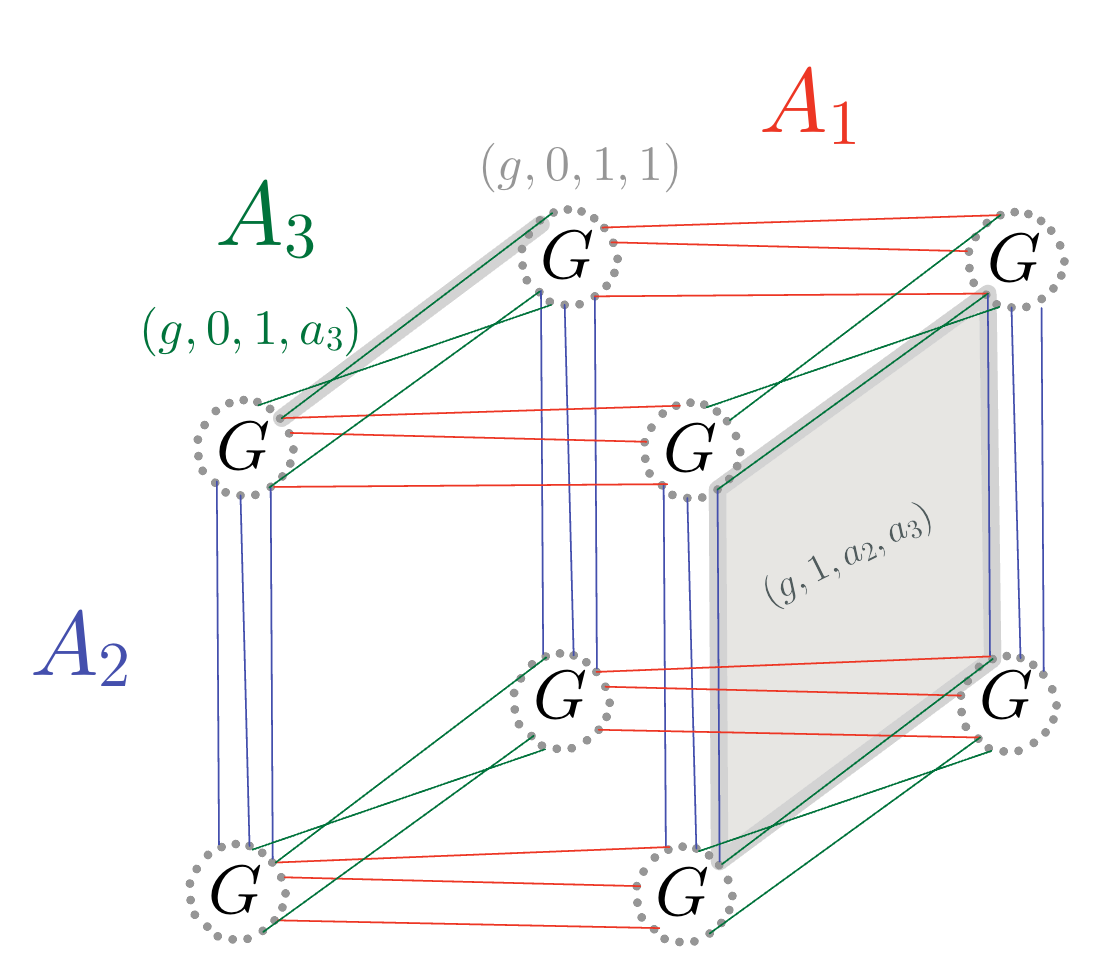
Figure 1: A cubical complex with $t=3$ and three sets of permutations $A_{1},A_{2},A_{3}$. The underlying graph can be seen to be $2^{t}=8$-partite. We label the faces as $(f_{0},f_{1},f_{2},f_{3})$.

Partial order

We introduce the following partial order on faces of $X$. This partial order is the one that is induced by set inclusion, when each face is seen as a set of vertices as in (8). Formally, given two faces $f,f^{\prime}$ and $j\in\{1,\ldots,t\}$ we write $f^{\prime}\mathrel{\ooalign{$\prec$\cr\hbox{$\cdot\mkern 0.5mu$}}}_{j}f$ if all the following hold:

• $f^{\prime}_{j}\in\{0,1\}$ while $f_{j}\in A_{j}$,

• $f_{i}=f^{\prime}_{i}$ for all $i\notin\{0,j\}$,

• $f^{\prime}_{0}=\begin{cases}f_{0}&f^{\prime}_{j}=0\\ f_{0}\cdot f_{j}&f^{\prime}_{j}=1\\ \end{cases}$ .

We sometimes suppress $j$ from the notation and write $f^{\prime}\mathrel{\ooalign{$\prec$\cr\hbox{$\cdot\mkern 0.5mu$}}}f$ to indicate that there is some $j$ for which $f^{\prime}\mathrel{\ooalign{$\prec$\cr\hbox{$\cdot\mkern 0.5mu$}}}_{j}f$. Note that if $f^{\prime}\mathrel{\ooalign{$\prec$\cr\hbox{$\cdot\mkern 0.5mu$}}}f$ then necessarily $f$ is one dimension higher than $f^{\prime}$. We also write $f^{\prime}\prec f$ if there is a sequence $f^{\prime}\mathrel{\ooalign{$\prec$\cr\hbox{$\cdot\mkern 0.5mu$}}}\cdots\mathrel{\ooalign{$\prec$\cr\hbox{$\cdot\mkern 0.5mu$}}}f$, and $f^{\prime}\preceq f$ if $f^{\prime}\prec f$ or $f^{\prime}=f$.

Lemma 3.1.

The relation $\prec$ defines a transitive graded partial order on faces. Moreover, with this relation $X$ is an incidence poset.

Proof.

The relation $\preceq$ is reflexive and transitive. It is antisymmetric because if $f^{\prime}\preceq f$ and $f\neq f^{\prime}$ then $f$ must be of dimension at least one more than $f^{\prime}$. To show that it is graded, we verify that the covering relation associated with $\preceq$ is precisely $\mathrel{\ooalign{$\prec$\cr\hbox{$\cdot\mkern 0.5mu$}}}$.

For the moreover part, note that if $f\mathrel{\ooalign{$\prec$\cr\hbox{$\cdot\mkern 0.5mu$}}}f^{\prime}\mathrel{\ooalign{$\prec$\cr\hbox{$\cdot\mkern 0.5mu$}}}f^{\prime\prime}$, then there are exactly two distinct positive $i\neq j$ such that $f^{\prime\prime}_{j}\neq f_{j}$ and $f^{\prime\prime}_{i}\neq f_{i}$, and this determines exactly two possible values for $f^{\prime}$. ∎

Definition 3.2.

Given the set $G$ and the sets of permutations $A_{1},\ldots,A_{t}$, we let $X(G;\{A_{i}\})$ denote the graded incidence poset $X=\cup_{0\leqslant k\leqslant t}X(k)$. Here the rank function is given by $\rho(f)=|\texttt{type}(f)|$, for $f\in X$.

We end the section by introducing convenient notation.

Incidence maps

The up incidence map $\mathfrak{u}$ takes a $k$-face $f$ to all $(k+1)$-faces that cover it,

$$\mathfrak{u}(f)=\left\{f^{\prime}\left|\;\vphantom{f^{\prime}f^{\prime}\mathrel{\ooalign{$\succ$\cr$\cdot$}}f}\right.f^{\prime}\mathrel{\ooalign{$\succ$\cr$\cdot$}}f\right\}\;,$$

and is naturally extended to sets of faces by taking unions. Similarly,

$$\mathfrak{d}(f)=\left\{f^{\prime}\left|\;\vphantom{f^{\prime}f^{\prime}\mathrel{\ooalign{$\prec$\cr\hbox{$\cdot\mkern 0.5mu$}}}f}\right.f^{\prime}\mathrel{\ooalign{$\prec$\cr\hbox{$\cdot\mkern 0.5mu$}}}f\right\}\;.$$

Links

The upwards link of a face $v\in X$ is a sub-complex consisting of all faces above $v$,

$$X_{\geqslant v}=\left\{f\in X\left|\;\vphantom{f\in Xf\succeq v}\right.f\succeq v\right\}.$$

Note that since the structure of $X$ is not simplicial, we do not remove $v$ from a face $f\succeq v$ when defining the link. Similarly, the downwards link of a face $v\in X$ is a sub-complex consisting of faces below $v$,

$$X_{\leqslant v}=\left\{f\in X\left|\;\vphantom{f\in Xf\preceq v}\right.f\preceq v\right\}.$$

For a subset $S\subseteq\{1,\ldots,t\}$ we denote $X_{\geqslant v}(S)=X_{\geqslant v}\cap X(S)$ and $X_{\leqslant v}(S)=X_{\leqslant v}\cap X(S)$. Similarly, $X_{\geqslant v}(k)=X_{\geqslant v}\cap X(k)$ and $X_{\leqslant v}(k)=X_{\leqslant v}\cap X(k)$.

3.2 Local coefficients

To each face we associate a local coefficient space. For $i\in\{1,\ldots,k\}$ let $m_{i}\geqslant 1$ be an integer and $\hat{A}_{i}=\{1,\ldots,m_{i}\}$. The local coefficient space associated with a face of type $S$ is the vector space

$$V_{S}=\mathbb{F}_{2}^{\prod_{j\in\overline{S}}\hat{A}_{j}}.$$ (9)

So the local coefficient space of a $t$-dimensional face is $V_{\{1,\ldots,t\}}=\mathbb{F}_{2}$, and the local coefficient space of a vertex is ($\prod_{j=1}^{t}m_{j}$)-dimensional. We write $V_{f}=V_{\texttt{type}(f)}$ for the local coefficient space of the face $f$, and $\mathcal{F}=\{V_{f}\}$ for the collection of local coefficient spaces.

For $i\in\{0,\ldots,t\}$ we denote by $C_{i}(X,\mathcal{F})$, or $C_{i}(X)$ for short, the vector space of $i$-chains, that assign to every $i$-face $f$ a “coefficient” from $V_{f}$:

$$C_{i}(X,\mathcal{F})\,=\,\bigoplus_{f\in X(i)}V_{f}\;.$$

Similarly, we use $C^{i}(X)$ to denote the $i$-cochains

$$C^{i}(X,\mathcal{F})\,=\,\bigoplus_{f\in X(i)}V_{f}^{*}\;,$$

where $V_{f}^{*}=\{g:V_{f}\to\mathbb{F}_{2}\}$ is the dual vector space. Throughout we fix an identification of each $V_{S}^{*}$ with $V_{S}$ through the use of a self-dual basis which we label $\{a:\,a\in\prod_{j\in\overline{S}}\hat{A}_{j}\}$, so $V_{f}^{*}\simeq V_{f}$ canonically.

Definition 3.3.

Given a set $G$ and subsets of permutations $A_{1},\ldots,A_{t}$ we let $C_{*}(G;\{A_{i}\};\{h_{i}\})$ be the length-$(t+1)$ chain complex

$$C_{*}(G;\{A_{i}\};\{h_{i}\})\,=\,\bigoplus_{i}C_{i}(X,\mathcal{F})\;.$$

We often write $C_{*}(X,\mathcal{F})$ or even $C_{*}(X)$ for this complex, when the parameters of the complex are clear from context. We use $C^{*}(X)=\oplus_{i}C^{i}(X)$ to denote the dual complex.

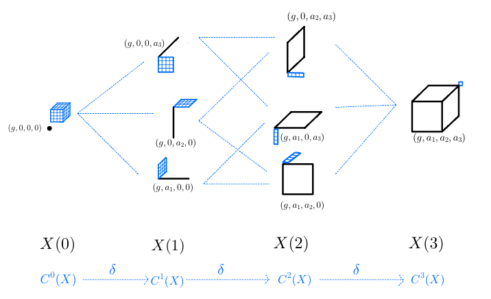
Figure 2: The co-chain complex, localized at a vertex $f=(g,0,0,0)$; with $t=3$. The geometric elements of $X_{\geqslant f}$ are drawn in black. The associated coefficient spaces are drawn in blue.

The (co-)boundary maps associated with $C_{*}$ are defined in the next sub-section. Before proceeding, we can already compute the dimension of the space of $i$-chains $C_{i}(X,\mathcal{F})$.

Lemma 3.4.

Let $C_{*}(X)=C_{*}(G;\{A_{i}\};\{h_{i}\})$, $0\leqslant i\leqslant t$ and $D_{i}=\mathrm{dim}\,C_{i}(X,\mathcal{F})$. Then

$$D_{i}\,=\,N\,n^{i}2^{t-i}\sum_{\begin{subarray}{c}T\subseteq\{1,\ldots,t\}\\ |T|=t-i\end{subarray}}\prod_{j\in T}m_{j}\;.$$

Proof.

We have that $D_{i}=\sum_{f\in X(i)}\mathrm{dim}V_{f}$. For each $f\in X(i)$, $|\texttt{type}(f)|=i$ and hence by (9), $\mathrm{dim}\,V_{f}=\prod_{j\notin\texttt{type}(f)}m_{j}$. Moreover, for $|S|=i$ we have $|X(S)|=Nn^{i}2^{t-i}$, where $N$ is to choose $g\in G$, $n^{i}$ is to choose $a_{j}$ for $j\in S$, and $2^{t-i}$ is to choose $b_{j}$ for $j\notin S$. ∎

3.3 (Co)boundary maps

For $i\in\{1,\ldots,t\}$ let $h_{i}\in\mathbb{F}_{2}^{m_{i}\times n}$. Assume that $m_{i}\leqslant n_{i}$ and that $h_{i}$ has full row rank, i.e.  the rows of $h_{i}$ are linearly independent. We index the rows of $h_{i}$ using the set $\hat{A}_{i}=\{1,\ldots,m_{i}\}$, and the columns of $h_{i}$ using the set $A_{i}$, and view $h_{i}$ as a linear map $h_{i}:\mathbb{F}_{2}^{A_{i}}\to\mathbb{F}_{2}^{\hat{A}_{i}}$.

Restriction and co-restriction maps

Given $i\notin\texttt{type}(f^{\prime})$ and $f^{\prime}\mathrel{\ooalign{$\prec$\cr\hbox{$\cdot\mkern 0.5mu$}}}_{i}f$, define the co-restriction map

$$\textrm{co-res}_{f^{\prime},f}\,:\quad V_{f^{\prime}}^{*}\to V_{f}^{*}$$

as follows. For any $z\in V_{f^{\prime}}^{*}$, $\textrm{co-res}_{f^{\prime},f}(z)$ is obtained by applying $I_{-i}\otimes h_{i}^{T}$, resulting in a vector in $\mathbb{F}_{2}^{(\prod_{j\not\in\texttt{type}(f^{\prime})}\hat{A}_{j})\times A_{i}}$, and then setting the $A_{i}$-coordinate to $f_{i}$. Formally,

$$\textrm{co-res}_{f^{\prime},f}(z)=\big{(}(I_{-i}\otimes h_{i}^{T})z\big{)}[\cdots,f_{i},\cdots]\;.$$ (10)

Similarly, for $i\in\texttt{type}(f^{\prime})$ and $f^{\prime}\mathrel{\ooalign{$\succ$\cr$\cdot$}}_{i}f$ define the restriction map

$$\textrm{res}_{f^{\prime},f}:V_{f^{\prime}}\to V_{f}$$

for any $z\in V_{f^{\prime}}$ by

$$\textrm{res}_{f^{\prime},f}(z)=z\otimes(h_{i}f^{\prime}_{i})\;,$$ (11)

which is an element of $\mathbb{F}_{2}^{\prod_{j\notin\texttt{type}(f^{\prime})}\hat{A}_{j}}\otimes\mathbb{F}_{2}^{\hat{A}_{i}}\cong\mathbb{F}_{2}^{\prod_{j\notin\texttt{type}(f)}\hat{A}_{j}}$. We abuse the notation and write $f^{\prime}_{i}$ as the canonical basis vector of $\mathbb{F}_{2}^{A_{i}}$ corresponding to $f^{\prime}_{i}\in A_{i}$. We verify below that the maps co-res and res are adjoint to each other (see (13)). We extend the notation by defining, for any sequence $f_{i}\mathrel{\ooalign{$\prec$\cr\hbox{$\cdot\mkern 0.5mu$}}}f_{i+1}\cdots\mathrel{\ooalign{$\prec$\cr\hbox{$\cdot\mkern 0.5mu$}}}f_{k}$ where $f_{j}\in X(j)$,

$$\textrm{res}_{f_{k},f_{i}}(z)\,=\,\textrm{res}_{f_{i+1},f_{i}}(\cdots\textrm{res}_{f_{k},f_{k-1}}((z)))\;.$$

We note that this leads to a well-defined quantity, i.e. $\textrm{res}_{f_{k},f_{i}}(z)$ is independent of the path $f_{i}\mathrel{\ooalign{$\prec$\cr\hbox{$\cdot\mkern 0.5mu$}}}f_{i+1}\cdots\mathrel{\ooalign{$\prec$\cr\hbox{$\cdot\mkern 0.5mu$}}}f_{k}$, as can easily be verified from the definition (11). This is because application of a linear map along different coordinates, or restriction on different coordinates, are operations that commute. A similar extension is performed to define co-restriction maps $\textrm{co-res}_{f^{\prime},f}$ for general $f^{\prime}\prec f$.

The coboundary map

The coboundary map $\delta:C^{*}(X)\to C^{*}(X)$ is defined as

$$\delta(z)(f)=\sum_{f^{\prime}\mathrel{\ooalign{$\prec$\cr\hbox{$\cdot\mkern 0.5mu$}}}f}\textrm{co-res}_{f^{\prime},f}(z(f^{\prime}))\;,$$ (12)

where $\textrm{co-res}_{f^{\prime},f}$ is as in (10). In words, at a face $f\in X$, we go over all faces $f^{\prime}$ below $f$ and map $z(f^{\prime})$ to an element in $V_{f}^{*}$ via the restriction map $\textrm{res}_{f^{\prime},f}$, and then sum all the contributions thus obtained.

The boundary map

The boundary map $\partial:C_{*}(X)\to C_{*}(X)$ is defined as

$$\partial(z)(f)=\sum_{f^{\prime}\mathrel{\ooalign{$\succ$\cr$\cdot$}}f}\textrm{res}_{f^{\prime},f}(z(f^{\prime})).$$

The next lemma shows that the map $\partial$ is the adjoint of the map $\delta$ with respect to the natural inner product on $C(X)$.

Lemma 3.5.

For any $z\in C_{*}(X)$ and $z^{\prime}\in C^{*}(X)$ it holds that

$$\langle z,\delta(z^{\prime})\rangle\,=\,\langle\partial(z),z^{\prime}\rangle\;.$$

Proof.

It is enough to verify the equality for $z\in V_{f}$ and $z^{\prime}\in V_{f^{\prime}}^{*}$. By definition $\delta:V_{f^{\prime}}^{*}\to\oplus_{f^{\prime\prime}\mathrel{\ooalign{$\succ$\cr$\cdot$}}f^{\prime}}V_{f^{\prime\prime}}^{*}$ and $\partial:V_{f}:\oplus_{f^{\prime\prime}\mathrel{\ooalign{$\prec$\cr\hbox{$\cdot\mkern 0.5mu$}}}f}V_{f^{\prime\prime}}$. Thus both sides of the equality are non-zero only if $f^{\prime}\mathrel{\ooalign{$\prec$\cr\hbox{$\cdot\mkern 0.5mu$}}}f$. Suppose that this is the case, and let $i$ be such that $\texttt{type}(f)=\texttt{type}(f^{\prime})\cup\{i\}$. It remains to verify that

$$\langle z,\textrm{co-res}_{f^{\prime},f}(z^{\prime})\rangle\,=\,\langle\textrm{res}_{f,f^{\prime}}(z),z^{\prime}\rangle\;.$$ (13)

According to (10)

$$\textrm{co-res}_{f^{\prime},f}(z^{\prime})=(I_{-i}\otimes h_{i}^{T})z^{\prime}[\cdots,f_{i},\cdots]\;,$$

and according to (11)

$$\textrm{res}_{f,f^{\prime}}(z)=z\otimes(h_{i}f_{i})\;.$$

Thus the left-hand side of (13) evaluates to

$$\langle z,(I_{-i}\otimes h_{i}^{T})z^{\prime}[\cdots,f_{i},\cdots]\rangle =\langle z\otimes f_{i},(I_{-i}\otimes h_{i}^{T})z^{\prime}\rangle$$

$$=\langle(I_{-i}\otimes h_{i})(z\otimes f_{i}),z^{\prime}\rangle$$

$$=\langle z\otimes(h_{i}f_{i}),z^{\prime}\rangle\;,$$

which matches the right-hand side. ∎

3.4 Statement of results

Having described our construction, we can state our main result about it.

Theorem 3.6.

Let $(G;\{A_{i}\})$ be a set and collections of permutations on it such that the graphs $\mathrm{Cay}(G,A_{i})$ are each $\lambda$-expanding (see Definition 5.4). Let $N=|G|$ and $n=|A_{1}|=\cdots=|A_{t}|$. Let $(h_{1},\ldots,h_{t})$ be a collection of matrices $h_{j}\in\mathbb{F}_{2}^{m_{j}\times n}$ such that the family $(h_{1},\ldots,h_{t})$ is two-way $\kappa$-robust (see Definition 4.9). Let $C=C_{*}(G;\{A_{j}\};\{h_{j}\})$ be the length-$(t+1)$ chain complex over $\mathbb{F}_{2}$ from Definition 3.3. Then there is a $c=\kappa^{t}\exp(-O(t^{2}))$ such that $C$ has the following properties.

1. The space $C_{k}$ of $k$-chains has dimension $D_{k}=N\ n^{k}2^{t-k}\sum_{\begin{subarray}{c}T\subseteq\{1,\ldots,t\}\\ |T|=t-k\end{subarray}}\prod_{j\in T}m_{j}$.

2. The co-chain complex $C^{*}$ has co-systolic distance $\mu_{\mathrm{cosyst}}(k)$ for every $0\leqslant k\leqslant t-1$ and co-cycle expansion $\varepsilon_{\mathrm{cocyc}}(k)$ for every $0\leqslant k\leqslant t-2$, where

   $$\mu_{\mathrm{cosyst}}(k)\,\geqslant\,\frac{c-\lambda}{2^{2t}n^{t}}|X(k)|\qquad\text{and}\qquad\varepsilon_{\mathrm{cocyc}}(k)\,\geqslant\,\frac{c-\lambda}{(2nt)^{2t+1}}\;.$$ (14)

3. The chain complex $C_{*}$ has systolic distance $\mu_{\mathrm{syst}}(k)$ for every $1\leqslant k\leqslant t$ and cycle expansion $\varepsilon_{\mathrm{cyc}}(k)$ for every $2\leqslant k\leqslant t$, where

   $$\mu_{\mathrm{syst}}(k) \geqslant\frac{1}{(2nt)^{t}}\mu_{\mathrm{cosyst}}(t-k)\;,$$

   $$\varepsilon_{\mathrm{cyc}}(k) \geqslant\min\Big{\{}\frac{\varepsilon_{\mathrm{cocyc}}(t-k)}{2(t^{2}2^{2t}n^{t+1})^{t}}\,,\;\frac{1}{(2nt)^{t}}\frac{\mu_{\mathrm{cosyst}}(t-k+1)}{|X(k)|}\Big{\}}\;.$$ (15)

We note that we did not attempt to overly optimize the bounds in Theorem 3.6; in particular the dependence on $t$ may be loose. To understand the bounds, one can consider that the main asymptotic parameter is $N=|G|$, which grows to infinity. We think of $t$ as a constant, such as $t=4$. The parameter $n$ is also ideally a constant; although for our construction below we have that $n=O(\log N)$. Choosing $n$ large enough allows us to take $\lambda$ sufficiently small compared to $\kappa$ so that the bounds in (14) are positive. For a constant $n$, these bounds are linear in the dimension, while for logarithmic $n$ they are smaller by a multiplicative inverse-polylogarithmic factor.

Proof of Theorem 3.6.

The first item is shown in Lemma 3.4.

For the second item, we first note the bound

$$\mathsf{d}_{\mathrm{coloc}}(k)\,\geqslant\,\frac{1-\lambda C_{1}}{C_{2}}|X(k)|\;,$$

valid for $0\leqslant k<t$, that follows from Proposition 6.1. The prefactor on the right-hand side can be re-written as

$$\frac{1-\lambda C_{1}}{C_{2}} =\big{(}1/C_{1}-\lambda\big{)}\frac{C_{1}}{C_{2}}$$

$$\geqslant\frac{1}{2^{2t}n^{t}}(\kappa^{t}2^{-4t^{2}}-\lambda)\;,$$

where the second line uses $t^{2}2^{2t}\leqslant 2^{3t^{2}}$ for $t\geqslant 1$. We then use Lemma 2.3 to conclude the claimed bounds. For $\varepsilon(k)$, we also use $|X(k+1)|/|X(k)|\leqslant 2nt$ and $|X_{\geqslant v}(k)|\leqslant(2n)^{t}$, which follow from Lemma 5.1. Finally, the bounds on $\tilde{\varepsilon}(k)$ and $\tilde{\mu}(k)$ follow immediately from Proposition 7.1. ∎

We can apply Theorem 3.6 to obtain quantum codes with parameters described in the following corollary. Since a quantum $CSS$ code can be defined from any length-$3$ complex, we have the choice to locate the qubits on the space of $k$-chains for any $i\in\{1,\ldots,t-1\}$. However, to obtain a bound on the local testability soundness of the quantum code, we need a complex of length at least $5$. To simplify the discussion of parameters we assume that, of the codes $\mathcal{C}_{i}=\ker h_{i}$, exactly $i$ have rate approaching $1$, and the remaining $(t-i)$ have rate approaching zero. This ensures that most of the dimension of the space $C_{i}$ is concentrated on a single type of $i$-face, and guarantees that the resulting code has positive dimension. Of course, other settings of parameters are possible.

Corollary 3.7.

With the same setup as in Theorem 3.6, assume $t\geqslant 4$ and fix $2\leqslant i\leqslant t-2$. Assume that the parameters $m_{1},\ldots,m_{t}$ and $n$ are chosen such that $m_{j}=\Theta(n)$ for all $j$, and furthermore $m_{j}/m_{j^{\prime}}$ is at least a sufficiently large constant (depending on $t$) when $j\in\{1,\ldots,i\}$ and $j^{\prime}\in\{i+1,\ldots,t\}$. Assume that, for these parameters there is a family $(h_{1},\ldots,h_{t})$ of two-way $\kappa$-robust codes, where $\kappa$ is small enough, as a function of $\lambda$ and $t$, so that the lower bounds in (14) are positive. Let $\mathcal{C}=CSS(\delta_{i},\partial_{i})$ be the CSS code associated with the space $C_{i}$ and the boundary and co-boundary operators on it. Then $\mathcal{C}$ is an $[\ell_{i},k_{i},d_{i}]$ CSS code with parity checks of weight $O(tn)$ and such that

1. $\ell_{i}=D_{i}=N\cdot\Theta(n)^{t}$,

2. $k_{i}=\Omega(\ell_{i})$,

3. $d_{i}=N\cdot(nt)^{-O(t)}\exp(-O(t^{2}))$.

Moreover, $\mathcal{C}$ is a qLTC with soundness $\rho\geqslant(nt)^{-O(t)}\exp(-O(t^{2}))$.

Proof.

The first item follows by definition of $\mathcal{C}$. For the second item, we lower bound $k_{i}$ by $D_{i}-D_{i-1}-D_{i+1}$, which is $\Omega(D_{i})$ given the assumption made on the parameters $m_{1},\ldots,m_{t}$ and $n$. As shown in Lemma 2.7 the distance is $d_{i}\geqslant\min\{\mu_{\mathrm{cosyst}}(i),\,\mu_{\mathrm{syst}}(i)\}$, giving the stated bound by Theorem 3.6. Similarly, the soundness is bounded using Lemma 2.7. ∎

As discussed earlier, if $n,t$ are both constant then we obtain a family of quantum LTC with constant weight parity checks, constant rate, relative distance and soundness. While the parameter $t$ can always be chosen to be a constant, we do not know how to construct the required $4$-dimensional cubical complex, with the right expansion properties, for $n$ constant. However, we can construct it for $n=O(\log N)$ by choosing $G=\mathbb{F}_{2}^{\log N}$ as discussed in the introduction.

4 The local chain

In this section we define a “local” chain complex $C(L_{S})$, for each subset $S\subseteq\{1,\ldots,t\}$. This chain complex will be used as a tool in the analysis of the complex $C_{*}(X,\mathcal{F})$ introduced in the previous section. In particular, as we will show in Lemma 4.2, the chain complex $C(L_{S})$ is isomorphic to the “local view” of $C_{*}(X,\mathcal{F})$ from any face $f$ such that $\texttt{type}(f)=\overline{S}$, i.e. the subcomplex $C_{*}(X_{\geqslant f};\mathcal{F})$. In Section 4.2 we introduce an important property of the local chain complex, robustness.

4.1 The complex

We start by defining a $1$-dimensional complex $L_{i}=L_{i}(0)\cup L_{i}(1)$, where $i\in\{1,\ldots,t\}$, as follows. There is a single $0$-dimensional face $L_{i}(0)=\{\emptyset\}$ and there are $n_{i}$ $1$-dimensional faces which we label using elements of $A_{i}$, $L_{i}(1)=A_{i}$. The incidence structure is the obvious one, $\emptyset\mathrel{\ooalign{$\prec$\cr\hbox{$\cdot\mkern 0.5mu$}}}a$ for any $a\in A_{i}$.

Next we introduce coefficient spaces $V_{\emptyset}=\mathbb{F}_{2}^{\hat{A}_{i}}$ and $V_{a}=\mathbb{F}_{2}$ for each $a\in A_{i}$. The coboundary map is defined, for $x\in\mathbb{F}_{2}^{\hat{A}_{i}}$ and (with a slight abuse of notation, which we will repeat) $a_{i}$ the $a_{i}$-th canonical basis vector of $\mathbb{F}_{2}^{A_{i}}$, as

$$\delta_{\{i\}}(x)(a_{i})\,=\,(h_{i}^{T}(x))(a_{i})\;.$$

The boundary map $\partial_{\{i\}}=\delta_{\{i\}}^{T}$ is then

$$\partial_{\{i\}}(y)(\emptyset)\,=\,h_{i}\,y\;,$$

where $y\in\oplus_{a}V_{a}\simeq\mathbb{F}_{2}^{A_{i}}$.

Above we used a subscript $\{i\}$ to distinguish them from the (co)boundary maps associated with the complex $C(X)$. We denote the resulting complex as $C(L_{\{i\}})$.

More generally, for $S\subseteq\{1,\ldots,t\}$ we define an $|S|$-dimensional complex $C(L_{S})$ as follows. For $k\in\{0,\ldots,|S|\}$ the $k$-faces are $L_{S}(k)=\cup_{T\subseteq S,|T|=k}L_{S}(T)$, where the faces $L_{S}(T)$ of type $T$ are in bijection with elements $f\in\mathbb{F}_{2}^{\prod_{i\in T}A_{i}}$. The incidence structure is given by $f^{\prime}\mathrel{\ooalign{$\succ$\cr$\cdot$}}f$ iff $f^{\prime}$ is of type $T^{\prime}$ such that $|T^{\prime}|=|T|+1$ and $T\subseteq T^{\prime}$. The local coefficient space associated to a face $f$ of type $T$ is $V_{f}=\mathbb{F}_{2}^{\prod_{i\in S-T}\hat{A}_{i}}$. For $x\in V_{f}$, the coboundary map is defined as

$$\delta_{S}(x)\,=\,\sum_{j\in S-T}(I_{-j}\otimes h_{j}^{T})(x)\,\in\bigoplus_{f^{\prime}\mathrel{\ooalign{$\succ$\cr$\cdot$}}f}V_{f^{\prime}}\;,$$

and the boundary map is

$$\partial_{S}(x)\,=\,\sum_{j\in T}(I_{-j}\otimes h_{j})(x)\,\in\bigoplus_{f^{\prime}\mathrel{\ooalign{$\prec$\cr\hbox{$\cdot\mkern 0.5mu$}}}f}V_{f^{\prime}}\;.$$

Remark 4.1.

One can verify that the complex $C(L_{S})$ is the homological product [BH14] of the $1$-dimensional complexes $C(L_{\{i\}})$, for $i\in S$. In particular, we see that $C_{0}(L_{S})\simeq\otimes_{i\in S}C_{0}(L_{\{i\}})$, $C_{1}(L_{S})\simeq\oplus_{i\in S}(C_{1}(L_{\{i\}})\otimes_{j\in S-\{i\}}C_{0}(L_{\{j\}}))$, etc.

Lemma 4.2 (Local and global).

For any face $f=[g;a,b]$ of type $S$ there is a natural isomorphism between $C(X_{\geqslant f})$ and $C(L_{\overline{S}})$. In particular, for every $T\subseteq\overline{S}$, $C(X_{\geqslant f}(S\cup T))\simeq C(L_{\overline{S}}(T))$.

Proof.

A face $g\in X_{\geqslant f}(S\cup T)$ is given by $a_{T}\in A_{T}$ and can be written as $g=(g_{i})$ where $g_{i}=\begin{cases}f_{i}&i\not\in T\\ a_{i}&i\in T\end{cases}$. In shorthand, $g=(f_{-T}||a_{T})$. By definition, for a face $g$ of type $S\cup T$, $V_{g}=\mathbb{F}_{2}^{\prod_{j\notin(S\cup T)}\hat{A}_{j}}=V_{S\cup T}$ so

$$C(X_{\geqslant f}(S\cup T))=\bigoplus_{g\in X_{\geqslant f}(S\cup T)}V_{g}=\bigoplus_{a\in A_{T}}V_{(f_{-T}||a_{T})}=\bigoplus_{a\in A_{T}}V_{S\cup T}\;.$$

An element of $C(X_{\geqslant f}(S\cup T))$ is thus a tuple $x=(x_{\bar{a}})_{\bar{a}\in A_{T}}$ where $x_{\bar{a}}\in\mathbb{F}_{2}^{\prod_{j\notin(S\cup T)}\hat{A}_{j}}$. Such a tuple is naturally identified with $x^{\prime}\in\mathbb{F}_{2}^{\prod_{j\in T}A_{j}\prod_{j\in\overline{S}\setminus T}\hat{A}_{j}}=C(L_{\overline{S}}(T))$ by setting $x^{\prime}_{\bar{a},\bar{a}^{\prime}}=(x_{\bar{a}})_{\bar{a}^{\prime}}$ for $\bar{a}\in\prod_{j\in T}A_{j}$ and $\bar{a}^{\prime}\in\prod_{j\in\overline{S}\setminus T}\hat{A}_{j}$.

It is easy to check that under this isomorphism the boundary and coboundary maps of $C(L_{\overline{S}})$ and of $C(X_{\geqslant f})$ coincide. ∎

We will use the following.

Lemma 4.3.

For any $S\subseteq\{1,\ldots,t\}$ the chain complex $C(L_{S})$ is exact at $i=0,\ldots,|S|-1$, i.e. for any $x\in C_{i}(L_{S})$ such that $\partial_{S}(x)=0$ there is a $y\in C_{i+1}(L_{S})$ such that $\partial_{S}(y)=x$.

Proof.

This follows from the Künneth formula, using that $C(L_{S})$ is the homological product of $1$-dimensional complexes $C(L_{\{i\}})$ which satisfy $\mathrm{dim}H_{0}(L_{\{i\}})=0$. ∎

Lemma 4.4.

For any $S\subseteq\{1,\ldots,t\}$ and for any $x\in C_{|S|}(L_{S})$ such that $\partial_{S}(x)=0$, $x$ must be in the tensor code $\bigotimes_{j\in S}\ker(h_{j})$.

Proof.

Observe that $C_{|S|}(L_{S})\cong\mathbb{F}_{2}^{\prod_{j\in S}A_{j}}$, so an element $x\in C_{|S|}(L_{S})$ is an $|S|$-dimensional tensor. The condition $\partial_{S}x=0$ for $x\in C_{|S|}(L_{S})$ implies that for every $j\in S$ and every $(a_{j})_{j\in S}\in\prod_{j\in S}A_{j}$, the column vector $x(a_{-j},\cdot)$ where we fix all coordinates except the $j$-th belongs to $\ker(h_{j})$. This is exactly the definition of the space $\bigotimes_{j\in S}\ker(h_{j})$. ∎

4.2 Robustness

Let $S\subseteq\{1,\ldots,t\}$ and $C(L_{S})$ be the dimension-$|S|$ complex described in the previous section. For $i\in S$ let

$$\mathcal{C}_{i}^{\perp}=\mathrm{im}\,(h_{i}^{T})\subseteq\mathbb{F}_{2}^{A_{i}}\;.$$

Let $d_{i}^{\perp}$ be the minimum distance of $\mathcal{C}_{i}^{\perp}$, i.e. $d_{i}^{\perp}=\min\{|x|_{H}:x\in\mathcal{C}_{i}^{\perp}\}$, where recall that $|\cdot|_{H}$ denotes the Hamming weight. For a $k$-face $f\in L_{S}(k)$ of type $T$ and $x\in V_{f}=\mathbb{F}_{2}^{\prod_{i\in S\setminus T}\hat{A}_{i}}$ we let $|x|=1_{x\neq 0}$. For $x\in C^{k}(L_{S})$ we let $|x|=\sum_{f\in L_{S}(k)}|x(f)|$, i.e. the number of faces $f$ such that $x(f)$ is nonzero. We refer to $|\cdot|$ as the block-(Hamming)-weight.

Definition 4.5.

Let $k\in\{1,\ldots,|S|\}$. An element $x\in C^{k}(L_{S})$ is called minimal if for any $y\in C^{k-1}(L_{S})$, $|x+\delta_{S}(y)|\geqslant|x|$.

Definition 4.6 (Robustness).

Let $S\subseteq\{1,\ldots,t\}$ and $\ell=|S|$. For $0\leqslant k\leqslant\ell-1$ let $\kappa_{\ell,k}$ be a positive real. We say that $C(L_{S})$ is $\kappa_{\ell,k}$-robust (implicitly, at level $k$) if for any $x\in C^{k}(L_{S})$ such that $x$ is minimal it holds that

$$|\delta_{S}(x)|\,\geqslant\,\kappa_{\ell,k}\,n\,|x|\;.$$

Remark 4.7.

For the case $|S|=1$, the condition of $x\in C^{0}(L_{S})$ being locally minimal is vacuous, because there are no $(-1)$-faces. Moreover, in that case $S=\{i\}$ for some $i$, $\delta_{S}(x)=h_{i}^{T}(x)$, $|x|=1_{x\neq 0}$ and $|\delta_{S}(x)|=|\delta_{S}(x)|_{H}$, the Hamming weight. Thus in this case the condition of robustness is equivalent to the condition of distance, i.e. for each $i\in\{1,\ldots,t\}$ we have that $L_{\{i\}}$ is $(d_{i}^{\perp}/n)$-robust, where $d_{i}^{\perp}$ is the distance of the dual code $\mathcal{C}_{i}^{\perp}$.

Remark 4.8.

The condition of $\kappa$-robustness is equivalent the notion of product-expansion from [KP22]. Furthermore, both notions are equivalent to co-boundary expansion of the complex $C(L_{S})$. For $k\in\{1,\ldots,|S|-1\}$ the co-boundary expansion coefficient $h^{k}(L_{S})$ is defined as

$$h^{k}(L_{S})\,=\,\min_{x\in C^{k}(L_{S})-\mathrm{im}\,(\delta_{S})}\frac{|\delta_{S}(x)|}{\min_{y\in\mathrm{im}\,(\delta_{S})}|x+y|}\;.$$

We have that $h^{k}(L_{S})\leqslant\kappa_{\ell,k}n$ because if $x$ is minimal then $\min_{y\in\mathrm{im}\,(\delta_{S})}|x+y|=|x|$. Conversely, if $x$ achieves the minimum in the definition of $h^{k}(L_{S})$ then $x^{\prime}=x+y$ for any $y\in\mathrm{im}\,(\delta_{S})$ that minimizes $|x+y|$ will be such that $|\delta_{S}(x^{\prime})|=h^{k}(L_{S})|x^{\prime}|$.

Definition 4.9.

Let $\kappa>0$. We say that the family $\{h_{i}\}$ is two-way $\kappa$-robust if the following conditions hold.

• When based on the matrices $\{h_{1},\ldots,h_{t}\}$, the complex $C(L_{S})$ is $\kappa$-robust for each $S\subseteq\{1,\ldots,t\}$ and at each level $k=0,\ldots,|S|-1$.

• When based on the matrices $\{h^{\perp}_{1},\ldots,h^{\perp}_{t}\}$, the complex $C(L_{S})$ is $\kappa$-robust for each $S\subseteq\{1,\ldots,t\}$ and at each level $k=0,\ldots,|S|-1$.

In [KP22, DHLV23] it is shown, via a probabilistic argument, that a pair of random parity check matrices is two-way $\kappa$-robust for some universal constant $\kappa>0$ that only depends on the rate of the codes. We conjecture that the same holds for arbitrary $t$-tuples, where the constant $\kappa$ is allowed to depend on $t$ and on the rates of the codes.

Conjecture 4.10 (Two-way robustness conjecture).

Let $t\geqslant 1$ and $\rho_{1},\ldots,\rho_{t}\in(0,1)$. Then there is a $\kappa>0$ (depending on the preceding parameters) such that a $t$-tuple of uniformly random parity check matrices $h_{i}\in\mathbb{F}_{2}^{(1-\rho_{i})n\times n}$is two-way $\kappa$-robust with probability that goes to $1$ as $n\to\infty$.

We note that the conjecture has been proven for $t=1$ and $t=2$. The case for $t=1$ is known as the Gilbert–Varshamov bound and the case for $t=2$ is shown recently in [KP22, DHLV23].

5 Expansion properties of the geometric complex

In this section we we define some random walks on $X$ that will play an important role in the analysis, and show that all these random walks have good expansion properties, assuming only that the “$1$-dimensional” random walks on the Cayley graphs $\mathrm{Cay}(G,A_{i})$ are expanding. Before proceeding, we start by formulating some useful incidence properties of the geometric complex $X$.

5.1 Incidence properties

Lemma 5.1.

Let $0\leqslant i\leqslant t$. Let $f\in X(i)$. Then

$$|\mathfrak{d}(f)|=2i\qquad\text{and}\qquad|\mathfrak{u}(f)|=(t-i)n\;.$$ (16)

More generally, if $0\leqslant\ell<i<k\leqslant t$ then

$$|X_{\geqslant f}(k)|=\binom{t-i}{k-i}n^{k-i}\qquad\text{and}\qquad|X_{\leqslant f}(\ell)|={i\choose\ell}2^{i-\ell}\;.$$ (17)

As a consequence,

$$|X(k)|\,=\,\frac{1}{2^{k}}\sum_{v\in X(0)}|X_{\geqslant v}(k)|\,=\,{t\choose k}2^{t-k}n^{k}|G|\;.$$

Proof.

An $i$-face is $f=[g;a,b]$ of type $S$ such that $|S|=i$. To specify an element in $\mathfrak{d}(f)$ we specify (i) an index $j\in S$ ($i$ choices) and (ii) a value $b_{i}$ ($2$ choices). To specify an element in $\mathfrak{u}(f)$ we specify (i) an index $j\notin S$ ($t-i$ choices) and (ii) a value for $a_{i}$ ($n$ choices).

More generally, to specify an element of $X_{\geqslant f}(k)$ we specify (i) a subset $S^{\prime}\subseteq\overline{S}$ of size $|S^{\prime}|=k-\ell$, and (ii) a value for $a_{S^{\prime}}$. To specify an element of $X_{\leqslant f}(\ell)$ we specify (i) a subset $S^{\prime}\subseteq S$ of size $|S^{\prime}|=i-\ell$ and (ii) an element $b\in\{0,1\}^{S^{\prime}}$.

Finally for the “consequence”, for the first equality note that each $f\in X(k)$ lies in $X_{\geqslant v}(k)$ for exactly $2^{k}$ vertices $v\in X(0)$. For the second equality, we have $|X(0)|=2^{t}|G|$. ∎

5.2 Markov operators

We recall some basic notation and facts.

Definition 5.2.

Let $V$ be a finite set. Let $\mathbb{R}^{V}$ denote the vector space of real functions on $V$ and $\langle\cdot,\cdot\rangle$ the standard inner product. For $M:\mathbb{R}^{V}\to\mathbb{R}^{V}$ linear we say that

1. $M$ is symmetric if $\langle M\phi,\psi\rangle=\langle\phi,M\psi\rangle$ for any $\phi,\psi\in\mathbb{R}^{V}$;

2. $M$ is Markov if $M\phi\geqslant 0$ whenever $\phi\geqslant 0$ (entrywise) and $M1_{V}=1_{V}$, with $1_{V}$ the constant one function;

3. $M$ is $\lambda$-expanding, for some $0<\lambda<1$, if $\langle M\phi,\phi\rangle\leqslant\lambda\langle\phi,\phi\rangle$ for all $\phi\in\mathbb{R}^{V}$ such that $\langle\phi,1_{V}\rangle=0$.

We will use the following well-known lemma.

Lemma 5.3.

Let $M:\mathbb{R}^{V}\to\mathbb{R}^{V}$ be a symmetric, Markov, $\lambda$-expanding linear operator. Then for any $0<\delta\leqslant 1$ and any $x\in\mathbb{R}^{V}$,

$$\langle x,Mx\rangle\leqslant\lambda\|x\|_{2}^{2}+\frac{\|x\|_{1}^{2}}{|V|}\;,$$

where $\|x\|_{1}=\sum_{i\in V}|x_{i}|$ and $\|x\|_{2}=(\sum_{i\in V}x_{i}^{2})^{1/2}$ denote the $1$- and $2$-norm of $x$ respectively.

Proof.

Decompose $x$ as $x=\alpha u+\beta v$, where $u,v$ are orthogonal vectors of norm $1$ such that $u$ is colinear to the all-$1$ vector. Then

$$\langle x,Mx\rangle =\alpha^{2}+\beta^{2}\langle v,Mv\rangle$$

$$\leqslant\alpha^{2}+\lambda\beta^{2}$$

$$=\alpha^{2}(1-\lambda)+\lambda\|x\|_{2}^{2}\;,$$

where the inequality uses that $v\bot u$ and the assumption that $M$ is $\lambda$-expanding. Moreover,

$$\alpha^{2} =|\langle x,u\rangle|^{2}$$

$$=\frac{\|x\|_{1}^{2}}{|V|}\;,$$

because $u_{i}=1/\sqrt{|V|}$ for all $i$. Combining both inequalities completes the proof. ∎

Given a graph $G=(V,E)$, we say that $G$ is $\lambda$-expanding if the Markov operator that is given by the normalized adjacency matrix of $G$ is $\lambda$-expanding. For each set $A_{j}$, we let $G_{j}=\mathrm{Cay}(G,A_{j})$ denote the graph whose vertex set is $V_{j}=G$, and such that there is an edge between $(g,g^{\prime})$ if and only if $g^{\prime}=g\cdot a_{j}$ for some $a_{j}\in A_{j}$. Since we assumed that $A_{j}$ is closed under inverse, $\mathrm{Cay}(G,A_{j})$ is an $n$-regular undirected graph (which for simplicity one may assume does not contain any self-loops, although our arguments extend verbatim if there are).

Definition 5.4.

For a set of permutations $A$ on $G$, we say that the pair $(G;A)$ is $\lambda$-expanding if the Markov operator $M:\mathbb{R}^{G}\to\mathbb{R}^{G}$ such that

$$M(e_{g})\,=\,\frac{1}{|A|}\sum_{a\in A}e_{g\cdot a}$$ (18)

is $\lambda$-expanding, where $e_{g}$ denotes the $g$-th canonical basis vector of $\mathbb{R}^{G}$.

Let $M_{j}$ be the Markov operator associated with the normalized adjacency matrix of $G_{j}=\mathrm{Cay}(G,A_{j})$ as in (18). Hereafter we define $\lambda$ as the maximum second eiganvalue among all $M_{j}$, i.e.

$$\lambda\,=\,\max_{1\leqslant j\leqslant t}\;\big{\{}\ \lambda_{2}(M_{j})\ \big{\}}\;,$$ (19)

where $\lambda_{2}(M_{j})$ denotes the second largest eigenvalue of $M_{j}$.

Let $D:\mathbb{R}^{X}\to\mathbb{R}^{X}$ be the normalized unsigned boundary operator, i.e.

$$D\phi(f)\,=\,\frac{1}{|\mathfrak{u}\{f\}|}\sum_{f^{\prime}\mathrel{\ooalign{$\succ$\cr$\cdot$}}f}\phi(f^{\prime})\;.$$

Note that $|\mathfrak{u}\{f\}|$ is independent of $f$ (see Lemma 5.1), and so this is a linear operator. Let $U$ be the normalized unsigned coboundary operator, i.e.

$$U\phi(f)\,=\,\frac{1}{|\mathfrak{d}\{f\}|}\sum_{f^{\prime}\mathrel{\ooalign{$\prec$\cr\hbox{$\cdot\mkern 0.5mu$}}}f}\phi(f^{\prime})\;.$$

Claim 5.5.

The operators $D$ and $U$ satisfy that for any $\ell$ and $\phi:X(\ell)\to\mathbb{R}$, $\phi^{\prime}:X(\ell-1)\to\mathbb{R}$,

$$\operatorname*{\mathbb{E}}_{f\in X(\ell-1)}\phi^{\prime}(f)D\phi(f)\,=\,\operatorname*{\mathbb{E}}_{f^{\prime}\in X(\ell)}U\phi^{\prime}(f^{\prime})\phi(f^{\prime})\;,$$

where both expectations are uniform.

Proof.

To verify this, for any $\phi,\phi^{\prime}$ we have

$$\frac{1}{X(\ell-1)}\sum_{f\in X(\ell-1)}\phi^{\prime}(f)D\phi(f) =\frac{1}{X(\ell-1)}\sum_{f\in X(\ell-1)}\frac{1}{\mathfrak{u}\{f\}}\sum_{f^{\prime}\mathrel{\ooalign{$\succ$\cr$\cdot$}}f}\phi^{\prime}(f)\phi(f^{\prime})$$

$$=\frac{1}{X(\ell)}\sum_{f^{\prime}\in X(\ell)}\frac{1}{\mathfrak{d}\{f^{\prime}\}}\sum_{f\mathrel{\ooalign{$\prec$\cr\hbox{$\cdot\mkern 0.5mu$}}}f^{\prime}}\phi^{\prime}(f)\phi(f^{\prime})$$

$$=\frac{1}{X(\ell)}\sum_{f^{\prime}\in X(\ell)}U\phi^{\prime}(f^{\prime})\phi(f^{\prime})\;.$$

Here the second line is because for any $f\mathrel{\ooalign{$\prec$\cr\hbox{$\cdot\mkern 0.5mu$}}}f^{\prime}$, $\frac{X(\ell-1)}{X(\ell)}=\frac{\mathfrak{d}\{f^{\prime}\}}{\mathfrak{u}\{f\}}$. ∎

5.3 Expanding random walks

We define and analyze some random walks on the vertex set $X(k)$.

Definition 5.6.

For $0\leqslant\ell\leqslant k$ define the following walk $W^{(k,\ell)}$ on $X(k)$. Starting at $f\in X(k)$,

1. Choose a uniformly random $v\in X(\ell)$ such that $v\in\mathfrak{d}^{(k-\ell)}\{f\}$. (If $\ell=k$ then set $v=f$.)

2. Write $v=[g;a,b]$ and $S=\texttt{type}(v)$. Choose a uniformly random $i\in\overline{S}$ and $a_{i}\in A_{i}$. Let $g^{\prime}=ga_{i}$, $a^{\prime}_{j}=a_{j}$ for $j\in S$, $b^{\prime}_{i}=1-b_{i}$, and $b^{\prime}_{j}=b_{j}$ for $j\in\overline{S}-\{i\}$. Let $v^{\prime}=[g^{\prime};a^{\prime},b^{\prime}]$.

3. Return a uniformly random $f^{\prime}\in\mathfrak{u}^{(k-\ell)}\{v^{\prime}\}$.

We write $W^{(k,\ell)}:\mathbb{R}^{X(k)}\to\mathbb{R}^{X(k)}$ for the Markov operator associated with this walk and $W^{(k,\ell)}_{adj}:\mathbb{R}^{X(k)}\to\mathbb{R}^{X(k)}$ for the adjacency matrix associated with this walk.

Definition 5.7.

Let $0\leqslant\ell\leqslant k<t$ and $v\in X(\ell)$. Recall the definition of the set

$$(\mathfrak{d}\circ\mathfrak{u})X_{\geqslant v}(k)=\big{\{}f\in X(k)\;\big{|}\;\exists f^{\prime}\in X_{\geqslant v}(k+1)\,,\;f\mathrel{\ooalign{$\prec$\cr\hbox{$\cdot\mkern 0.5mu$}}}f^{\prime}\big{\}}\;.$$

In words, these are $k$-faces that are included in a $(k+1)$-face that contains $v$. Such faces can either contain $v$, or intersect but not contain $v$, or not intersect $v$. We write the set of $k$-faces that intersect but do not contain $v$ as

$$\mathrm{Nb}_{v}(k)=\big{\{}f\in X(k)\;\big{|}\;\exists f^{\prime}\in X_{\geqslant v}(k+1)\,,\;f\mathrel{\ooalign{$\prec$\cr\hbox{$\cdot\mkern 0.5mu$}}}f^{\prime}\,,\;f\cap v\neq\emptyset,v\nprec f\big{\}}\;,$$

and those that do not intersect $v$ as

$$\mathrm{Op}_{v}(k)=\big{\{}f\in X(k)\;\big{|}\;\exists f^{\prime}\in X_{\geqslant v}(k+1)\,,\;f\mathrel{\ooalign{$\prec$\cr\hbox{$\cdot\mkern 0.5mu$}}}f^{\prime}\,,\;f\cap v=\emptyset\big{\}}\;.$$

From the definition, it is clear that

$$(\mathfrak{d}\circ\mathfrak{u})X_{\geqslant v}(k)\,=\,X_{\geqslant v}(k)\cup\mathrm{Nb}_{v}(k)\cup\mathrm{Op}_{v}(k)\;.$$ (20)

The following lemma states a useful “covering” property for the neighborhoods $\mathrm{Nb}_{v}(k)$. First, for any $0\leqslant\ell<k<t$ we define

$$a_{k,\ell}\,=\,\max_{\begin{subarray}{c}v_{\ell}\in X(\ell),\,v_{k},v^{\prime}_{k}\in X(k):\\ v_{\ell}\prec v_{k},\,v_{\ell}\prec v^{\prime}_{k}\end{subarray}}\big{|}\big{\{}v_{\ell+1}\in X(\ell+1):\,v_{\ell}\prec v_{\ell+1}\preceq v_{k}\,\hbox{ and }\,v_{k}^{\prime}\in\mathrm{Nb}_{v_{\ell+1}}(k)\big{\}}\big{|}\;.$$ (21)

We observe the crude bound

$$a_{k,\ell}\,\leqslant\,|X_{\leqslant v_{k}}(\ell+1)|\,\leqslant\,2^{t}$$ (22)

for all $\ell,k$. Here the first inequality is because $v_{\ell+1}$ in (21) must be in $X_{\geqslant v_{k}}(\ell+1)$, and the second inequality is by Lemma 5.1. Furthermore, we observe the following claim (which will not be used in the proof).

Claim 5.8.

If $k=t-1$ then $a_{t-1,\ell}=1$ for all $\ell<t-1$.

Proof.

Fix $v_{\ell}\in X(\ell)$ and $v_{k},v^{\prime}_{k}\in X(k)$ such that $v_{\ell}\prec v_{k}$ and $v_{\ell}\prec v^{\prime}_{k}$. We first show that any $v_{\ell+1}\in X(\ell+1)$ such that $v_{\ell}\prec v_{\ell+1}\preceq v_{k}$ and $v^{\prime}_{k}\in\mathrm{Nb}_{v_{\ell+1}}(k)$ has $\texttt{type}(v_{\ell+1})=\texttt{type}(v_{\ell})\cup([t]\setminus\texttt{type}(v^{\prime}_{k}))$. This is because using the first condition necessarily $\texttt{type}(v_{\ell+1})\supseteq\texttt{type}(v_{\ell})$ and has exactly one more element; furthermore, using the second condition that element must be the unique element of $[t]$ that is not in $\texttt{type}(v^{\prime}_{k})$. Once its type has been fixed, $v_{\ell+1}$ is uniquely determined by the condition $v_{\ell}\prec v_{\ell+1}\preceq v_{k}$. ∎

Lemma 5.9.

For all $v_{k}\in X(k)$ and $\ell<k$,

$$\bigsqcup_{v_{\ell+1}\preceq v_{k}}\mathrm{Nb}_{v_{\ell+1}}(k)\,\subseteq\,a_{k,\ell}\cdot\bigsqcup_{v_{\ell}\prec v_{k}}X_{\geqslant v_{\ell}}(k)\;,$$

where $\sqcup$ denotes the union of multisets, i.e. elements are counted with multiplicity, and $a\cdot S$ is all elements of the multiset $S$ with multiplicity multiplied by $a$.

Proof.

Let $v_{k}\in X(k)$. For $v_{\ell+1}\in X(\ell+1)$, each face $v_{k}^{\prime}\in\mathrm{Nb}_{v_{\ell+1}}(k)$ intersects $v_{\ell+1}$ on some $\ell$-dimensional face. This is because, since $\mathrm{Nb}_{v_{\ell+1}}(k)\subseteq(\mathfrak{d}\circ\mathfrak{u})X_{\geqslant v_{\ell+1}}(k)$ by definition, the types of $v_{k}$ and $v_{k}^{\prime}$ must differ by at most one element. Additionally, the intersection could not be an $\ell+1$-dimensional face, otherwise $v_{\ell+1}\preceq v_{k}^{\prime}$ which implies $v_{k}^{\prime}\notin\mathrm{Nb}_{v_{\ell+1}}(k)$. Therefore,

$$\bigsqcup_{v_{\ell+1}\preceq v_{k}}\mathrm{Nb}_{v_{\ell+1}}(k) =\bigsqcup_{v_{\ell+1}\preceq v_{k}}\bigsqcup_{v_{k}^{\prime}\in\mathrm{Nb}_{v_{\ell+1}}(k)}\{v_{k}^{\prime}\}$$

$$=\bigsqcup_{v_{\ell+1}\preceq v_{k}}\bigsqcup_{v_{k}^{\prime}\in\mathrm{Nb}_{v_{\ell+1}}(k)}\bigsqcup_{v_{\ell}\prec v_{\ell+1}}1_{v_{\ell+1}\cap v_{k}^{\prime}=v_{\ell}}\cdot\{v_{k}^{\prime}\}$$

$$=\bigsqcup_{v_{\ell}\prec v_{k}}\bigsqcup_{v_{k}^{\prime}\succ v_{\ell}}\bigsqcup_{v_{\ell+1}:v_{\ell}\prec v_{\ell+1}\preceq v_{k}}1_{v_{\ell+1}\cap v_{k}^{\prime}=v_{\ell}}\cdot 1_{v_{k}^{\prime}\in\mathrm{Nb}_{v_{\ell+1}}(k)}\cdot\{v_{k}^{\prime}\}$$

$$\subseteq\bigsqcup_{v_{\ell}\prec v_{k}}\bigsqcup_{v_{k}^{\prime}\succ v_{\ell}}a_{k,\ell}\cdot\{v_{k}^{\prime}\}$$

$$=a_{k,\ell}\cdot\bigsqcup_{v_{\ell}\prec v_{k}}X_{\geqslant v_{\ell}}(k)\;.$$

∎

Definition 5.10.

For $0\leqslant\ell\leqslant k$ define the following walk $\mathrm{Op}^{(k,\ell)}$ on $X(k)$. Starting at $f\in X(k)$,

1. Choose a uniformly random $v\in X(\ell)$ such that $v\in\mathfrak{d}^{(k-\ell)}\{f\}$. (If $\ell=k$ then set $v=f$.)

2. Return a uniformly random $f^{\prime}\in\mathrm{Op}_{v}(k)$.

We write $\mathrm{Op}^{(k,\ell)}:\mathbb{R}^{X(k)}\to\mathbb{R}^{X(k)}$ for the Markov operator associated with this walk and $\mathrm{Op}^{(k,\ell)}_{adj}:\mathbb{R}^{X(k)}\to\mathbb{R}^{X(k)}$ for the adjacency matrix associated with this walk.

The random walk $\mathrm{Op}^{(k,\ell)}$ is used in the proof of co-systolic distance. For the analysis, it will be convenient to relate it to the walk $W^{(k,\ell)}$. This is done through the following claim.

Claim 5.11.

$$\langle 1_{\mathcal{A}},\mathrm{Op}^{(k,\ell)}_{adj}1_{\mathcal{A}}\rangle\,\leqslant\,\langle 1_{\mathcal{A}},W^{(k,\ell)}_{adj}1_{\mathcal{A}}\rangle\,=\,{k\choose\ell}{t-\ell\choose k-\ell}(t-\ell)2^{k-\ell}n^{k+1-\ell}\langle 1_{\mathcal{A}},W^{(k,\ell)}1_{\mathcal{A}}\rangle\;.$$

Proof.

It is not hard to check that $\langle 1_{\mathcal{A}},\mathrm{Op}^{(k,\ell)}_{adj}1_{\mathcal{A}}\rangle\leqslant\langle 1_{\mathcal{A}},W^{(k,\ell)}_{adj}1_{\mathcal{A}}\rangle$ from the definitions. To show that $W^{(k,\ell)}_{adj}={k\choose\ell}{t-\ell\choose k-\ell}(t-\ell)2^{k-\ell}n^{k+1-\ell}W^{(k,\ell)}$, we observe that the normalization factor for $W^{(k,\ell)}$ is, using notations from Definition 5.6,

$$|X_{\leqslant f}(\ell)||\overline{S}||A_{i}||X_{\geqslant v^{\prime}}(k)| =\left({k\choose\ell}2^{k-\ell}\right)(t-\ell)(n)\left({t-\ell\choose k-\ell}n^{k-\ell}\right)$$

$$={k\choose\ell}{t-\ell\choose k-\ell}(t-\ell)2^{k-\ell}n^{k+1-\ell}\;,$$

where the first equality uses bounds from Lemma 5.1. ∎

One would hope that $W^{(k,\ell)}$ has spectral expansion. However, $W^{(k,\ell)}$ shares similarities to the random walk on a hypercube, which is not a good spectral expander. Nevertheless, $W^{(k,\ell)}$ has small-set expansion, as the next lemma shows.

Lemma 5.12.

Assume that for each $j\in\{1,\ldots,t\}$ the pair $(G;A_{j})$ is $\lambda$-expanding. Let $0\leqslant\ell\leqslant k$ and $\mathcal{A}\subseteq X(k)$. Then

$$\langle 1_{\mathcal{A}},W^{(k,\ell)}1_{\mathcal{A}}\rangle\,\leqslant\,\lambda|\mathcal{A}|+{t\choose\ell}2^{t-\ell-1}n^{\ell}\frac{|\mathcal{A}|^{2}}{|X(k)|}\;.$$ (23)

Note that $\lambda|\mathcal{A}|$ is the dominating term when $\frac{|\mathcal{A}|}{|X(k)|}$ is a small constant.

Proof.

Let $M$ be the Markov operator associated to step 2 of the walk $W^{(k,\ell)}$ introduced in Definition 5.6. We first discuss the structural properties of $M$. Notice that the type of the face does not change after a step of the walk $M$. Thus, $M$ is a direct sum of Markov operators $M_{S}$, for $S$ a subset of size $\ell$, each of which corresponds to the restriction of $M$ to faces of type $S$. $M_{S}$ can be further decomposed into a sum of operators $M_{S,i}$, for $i\in\overline{S}$, associated to the walk in the $i$-th direction. This decomposition is not a direct sum, but an average. Finally, $M_{S,i}$ is isomorphic to the direct sum of $n^{\ell}2^{t-\ell-1}$ disjoint copies of the walk on the double cover of $\mathrm{Cay}(G,A_{i})$. This is because $a_{S}$ and $b_{\overline{S}-i}$ are not changed by $M_{S,i}$; only $g$ and $b_{i}$ are. Denote the random walk on the double cover of $\mathrm{Cay}(G,A_{i})$ as $P_{i}$. To summarize,

$$M\,=\,\sum_{|S|=\ell}M_{S}\;,\qquad M_{S}\,=\,\frac{1}{t-\ell}\sum_{i\in\overline{S}}M_{S,i}\;,\qquad\text{and}\qquad M_{S,i}\,=\,P_{i}^{\oplus n^{\ell}2^{t-\ell-1}}\;.$$

We now prove the lemma. For $P_{i}$, by applying the expander mixing lemma, Lemma 5.3, on the double cover of $\mathrm{Cay}(G,A_{i})$ we have

$$\langle x,P_{i}x\rangle\,\leqslant\,\lambda\lVert x\rVert_{2}^{2}+\frac{\lVert x\rVert_{1}^{2}}{2|G|}$$

for all real functions $x$ on the vertices. Because $M_{S,i}$ is a direct sum of $P_{i}$, the same inequality carries over:

$$\langle x,M_{S,i}x\rangle\,\leqslant\,\lambda\lVert x\rVert_{2}^{2}+\frac{\lVert x\rVert_{1}^{2}}{2|G|}\;.$$

Because $M_{S}=\frac{1}{t-\ell}\sum_{i\in\overline{S}}M_{S,i}$,

$$\langle x,M_{S}x\rangle\,=\,\frac{1}{t-\ell}\sum_{i\in\overline{S}}\langle x,M_{S,i}x\rangle\,\leqslant\,\lambda\lVert x\rVert_{2}^{2}+\frac{\lVert x\rVert_{1}^{2}}{2|G|}\;.$$

Finally, since $M$ is a direct sum of $M_{S}$, we obtain that for any real function $x$ on the faces $X(\ell)$,

$$\langle x,Mx\rangle\,\leqslant\,\lambda\lVert x\rVert_{2}^{2}+\frac{\lVert x\rVert_{1}^{2}}{2|G|}\;.$$ (24)

We can now evaluate

$$\langle 1_{\mathcal{A}},W^{(k,\ell)}1_{\mathcal{A}}\rangle =\langle 1_{\mathcal{A}},U^{\circ(k-\ell)}MD^{\circ(k-\ell)}1_{\mathcal{A}}\rangle$$

$$=\frac{|X(k)|}{|X(\ell)|}\langle D^{\circ(k-\ell)}1_{\mathcal{A}},MD^{\circ(k-\ell)}1_{\mathcal{A}}\rangle$$

$$\leqslant\frac{|X(k)|}{|X(\ell)|}\lambda\langle D^{\circ(k-\ell)}1_{\mathcal{A}},D^{\circ(k-\ell)}1_{\mathcal{A}}\rangle+\frac{|X(k)|}{|X(\ell)|}\frac{\langle 1_{X(\ell)},D^{\circ(k-\ell)}1_{\mathcal{A}}\rangle^{2}}{2|G|}$$

$$=\frac{|X(k)|}{|X(\ell)|}\lambda\langle D^{\circ(k-\ell)}1_{\mathcal{A}},D^{\circ(k-\ell)}1_{\mathcal{A}}\rangle+\frac{|X(k)|}{|X(\ell)|}\frac{\langle D^{\circ(k-\ell)}1_{X(k)},D^{\circ(k-\ell)}1_{\mathcal{A}}\rangle^{2}}{2|G|}$$

$$\leqslant\lambda\langle 1_{\mathcal{A}},1_{\mathcal{A}}\rangle+\frac{|X(\ell)|}{|X(k)|}\frac{\langle 1_{X(k)},1_{\mathcal{A}}\rangle^{2}}{2|G|}$$

$$\leqslant\lambda|\mathcal{A}|+\frac{|X(\ell)|}{|X(k)|}\frac{|\mathcal{A}|^{2}}{2|G|}$$

$$\leqslant\lambda|\mathcal{A}|+\frac{{t\choose\ell}2^{t-\ell}n^{\ell}|G|}{2|G|}\frac{|\mathcal{A}|^{2}}{|X(k)|}\;.$$

Here the second line uses Claim 5.5. The third line uses (24) and the fact that $D^{\circ(k-\ell)}1_{\mathcal{A}}$ has nonnegative entries, which implies that $\lVert D^{\circ(k-\ell)}1_{\mathcal{A}}\rVert_{1}=\langle 1_{X(\ell)},D^{\circ(k-\ell)}1_{\mathcal{A}}\rangle$. The fourth and fifth lines use that $D$ is an averaging operator, and the regularity properties of the complex. The last line uses $|X(\ell)|={t\choose\ell}2^{t-\ell}n^{\ell}|G|$ by Lemma 5.1. ∎

6 Locally co-minimal distance

The main result of this section is that for any $0\leqslant k<t$, the co-chain complex $C^{*}(X,\mathcal{F})$ is a co-systolic expander in dimension $k$ according to Definition 2.1, assuming the expansion parameter $\lambda$ (see (19)) is small enough as a function of $n,t$ and the robustness parameters introduced in Section 4.2.

Quantitatively, we first prove a lower bound on the locally co-minimal distance of $C^{k}(X)$. This is introduced in Section 2.1. For convenience we recall the definition

$$\mathsf{d}_{\mathrm{coloc}}(k)\,=\,\min\big{\{}|x|\,:\,x\in\ker\delta_{k}-\{0\},\,\text{$x$ is locally co-minimal}\big{\}}\;.$$ (25)

Bounds on the co-cycle expansion parameters follow immediately from a lower bound on $\mathsf{d}_{\mathrm{coloc}}(k)$, as shown in Lemma 2.3.

Proposition 6.1.

Let $0\leqslant k<t$. Assume that there exists $\kappa_{t-i,k-i}>0$, for each $0\leqslant i\leqslant k$, such that for each $S\subseteq\{1,\ldots,t\}$ with $|S|=t-i$ the local chain complex $C(L_{S})$ is $\kappa_{t-i,k-i}$-robust (at level $k-i$) according to Definition 4.6. Then

$$\mathsf{d}_{\mathrm{coloc}}(k)\,\geqslant\,\frac{1-\lambda C_{1}}{C_{2}}|X(k)|\;,$$

where

$$C_{1}\,=\,\frac{t^{2}2^{t^{2}+3t}}{\prod_{i=0}^{k}\kappa_{t-i,k-i}}\qquad\text{and}\qquad C_{2}\,=\,\frac{t^{2}2^{t^{2}+5t}n^{t}}{\prod_{i=0}^{k}\kappa_{t-i,k-i}}\;.$$

Remark 6.2.

The constants $C_{1}$ and $C_{2}$ are simplifications of constants $C_{1}^{\prime}$ and $C_{2}^{\prime}$ which provide a slightly tighter bound, see (30) in the proof of Proposition 6.1, where the coefficients $a_{k,\ell}$ are defined in (21). To simplify these bounds, we we apply the estimate $a_{k,\ell}\leqslant 2^{t}$ from (22). Then,

$$C^{\prime}_{1}=\sum_{\ell=0}^{k}\frac{{k\choose\ell}{t-\ell\choose k-\ell}(t-\ell)2^{k-\ell}\prod_{i=\ell}^{k-1}a_{k,i}}{\prod_{i=\ell}^{k}\kappa_{t-i,k-i}}\leqslant t\frac{2^{t}2^{t}t2^{t}(2^{t})^{t}}{\prod_{i=0}^{k}\kappa_{t-i,k-i}}=C_{1}\;,$$

and

$$C^{\prime}_{2}=\sum_{\ell=0}^{k}\frac{{t\choose\ell}2^{t-\ell-1}n^{\ell}{k\choose\ell}{t-\ell\choose k-\ell}(t-\ell)2^{k-\ell}\prod_{i=\ell}^{k-1}a_{k,i}}{\prod_{i=\ell}^{k}\kappa_{t-i,k-i}}\leqslant t\frac{2^{t}2^{t}n^{t}2^{t}2^{t}t2^{t}(2^{t})^{t}}{\prod_{i=0}^{k}\kappa_{t-i,k-i}}=C_{2}\;.$$

Remark 6.3.

We explicitly work out the requirements on $\lambda$ and the $\kappa_{\ell,k}$ that suffice to guarantee a linear (in $X(k)$) co-systolic distance, i.e. such that $1-\lambda C^{\prime}_{1}>0$, for certain cases of interest. We use the shorthand $\kappa_{i}=\kappa_{i,i-1}$ for the robustness at the last level of the chain complex. Note that when $k=t-1$, by Claim 5.8 we have that $a_{k,i}=1$.

When $t=2,k=1$ the sufficient condition is

$$\frac{1}{\kappa_{1}}+\frac{8}{\kappa_{1}\kappa_{2}}\,<\,\frac{1}{\lambda}\;.$$ (26)

This is the sufficient condition for obtaining good qLDPC using our construction. When $t=4,k=3$ the sufficient condition is

$$\frac{1}{\kappa_{1}}+\frac{24}{\kappa_{1}\kappa_{2}}+\frac{108}{\kappa_{1}\kappa_{2}\kappa_{3}}+\frac{128}{\kappa_{1}\kappa_{2}\kappa_{3}\kappa_{4}}<\frac{1}{\lambda}\;.$$ (27)

This is the sufficient condition for obtaining good (again, up to polylog factors) qLTC using our construction.

Let $k<t$ and $x\in C^{k}(X)$ be such that $\delta(x)=0$. For $f\in X(k)$ we say that $f$ is active if the projection $x(f)$ of $x$ on $V_{f}$ is nonzero. Let $\mathcal{A}\subseteq X(k)$ be the set of active faces. At a high level, the proof of Proposition 6.1 amounts to showing that, whenever $x$ is locally co-minimal, the set $\mathcal{A}$ only expands a little under a suitable expanding random walk, which is based on the robustness of the local codes. However, when $\mathcal{A}\neq\emptyset$, the spectral expansion of the graph implies to have such small expansion, the set must be large, leading to a lower bound on $|x|$.

Proof of Proposition 6.1.

Let $x\in C^{k}(X)$ be such that $\delta(x)=0$ and $x$ is locally co-minimal. We start with a preliminary claim, which shows that the locally co-minimal condition implies the following.

Claim 6.4.

Let $\ell<k$ and $v\in X(\ell)$. Using the isomorphism from Lemma 4.2, the restriction $x(X_{\geqslant v}(k))$ can be seen as a $(k-\ell)$-chain of the dimension $(t-\ell)$ complex $C(L_{\overline{S}})$ where $S=\texttt{type}\,{v}$. Let $z$ be that element. Then $z$ is minimal (according to Definition 4.5).

Proof.

It suffices to show that

$$\forall y\text{ supported on }X_{\geqslant v}(k-1)\;,\qquad\big{|}x\big{(}X_{\geqslant v}(k)\big{)}+\delta_{\overline{S}}(y)\big{|}\,\geqslant\,\big{|}x\big{(}X_{\geqslant v}(k)\big{)}\big{|}\;.$$

Let $y$ be supported on $X_{\geqslant v}(k-1)$. Then $\delta_{\overline{S}}(y)=\delta(y)(X_{\geqslant v}(k))$. Thus $x+\delta(y)$ decomposes as a sum

$$x+\delta(y)\,=\,\big{(}x\big{(}X_{\geqslant v}(k)\big{)}+\delta_{\overline{S}}(y)\big{)}+\big{(}x-x\big{(}X_{\geqslant v}(k)\big{)}\big{)}\;,$$

where the two elements on the right-hand side are supported on a disjoint set of faces: $X_{\geqslant v}(k)$ for the first and its complement in $X(k)$ for the second. Thus

$$\big{|}x\big{(}X_{\geqslant v}(k)\big{)}+\delta_{\overline{S}}(y)\big{|} =\big{|}x+\delta(y)\big{|}-\big{|}x-x\big{(}X_{\geqslant v}(k)\big{)}\big{|}$$

$$\geqslant\big{|}x\big{|}-\big{|}x-x\big{(}X_{\geqslant v}(k)\big{)}\big{|}$$

$$=\big{|}x\big{(}X_{\geqslant v}(k)\big{)}\big{|}\;,$$

where the second line uses local minimality of $x$ (according to Definition 2.2). ∎

The key step in the proof is the following claim, which uses the robustness assumption on the local chain complex $C(L_{S})$.

Claim 6.5.

Let $\ell\leqslant k$. For all $v\in X(\ell)$,

$$\kappa_{t-\ell,k-\ell}n\ |x(X_{\geqslant v}(k))|\,\leqslant\,|x(\mathrm{Op}_{v}(k))|+|x(\mathrm{Nb}_{v}(k))|\;.$$ (28)

Proof.

We apply the robustness condition to $z=x(X_{\geqslant v}(k))$, seen as a $(k-\ell)$-chain of $C(L_{\overline{S}})$ where $S=\texttt{type}\,{v}$. By Claim 6.4, $z$ is minimal. Therefore,

$$\kappa_{t-\ell,k-\ell}n\ |x(X_{\geqslant v}(k))|\,\leqslant\,|\delta_{\overline{S}}(x(X_{\geqslant v}(k)))|\;.$$

Because $\delta x=0$ and $(\mathfrak{d}\circ\mathfrak{u})X_{\geqslant v}(k)=X_{\geqslant v}(k)\cup\mathrm{Nb}_{v}(k)\cup\mathrm{Op}_{v}(k)$ by (20), each nonzero entry in $\delta_{\overline{S}}(x(X_{\geqslant v}(k)))$ has to be canceled by some nonzero entries in $x(\mathrm{Op}_{v}(k))$ or $x(\mathrm{Nb}_{v}(k))$. Hence,

$$|\delta_{\overline{S}}(x(X_{\geqslant v}(k)))|\leqslant|x(\mathrm{Op}_{v}(k))|+|x(\mathrm{Nb}_{v}(k))|\;.$$

Combining the two inequalities above gives (28). ∎

Informally, Claim 6.5 for $\ell=k$ states that whenever a face $v\in X(k)$ is active, i.e. $|x(X_{\geqslant v}(k))|=|x(v)|=1$, it must have either many neighbors that are active, or many opposite neighbors that are active. In the latter case, we can make a step according to the random walk $\mathrm{Op}^{(k,k)}$ introduced in Defition 5.10, and use the expansion properties of that walk to conclude. However, in the former case a step to $\mathrm{Nb}_{v}(k)$ would not be expanding (because neighbors share a lower-dimensional face). In that case, we instead first sample a lower-dimensional sub-face of $v$, and move to an opposite neighbor of the latter face. The following claim analyses this recursive process. Recall the definition of the coefficients $a_{k,\ell}$ in (21).

Claim 6.6.

Let $v_{k}\in X(k)$. Then

$$|x(v_{k})|\,\leqslant\,\sum_{\ell=0}^{k}\sum_{v_{\ell}\preceq v_{k}}\frac{\prod_{i=\ell}^{k-1}a_{k,i}}{\prod_{i=\ell}^{k}(\kappa_{t-i,k-i}n)}|x(\mathrm{Op}_{v_{\ell}}(k))|\;.$$ (29)

Proof.

We apply Claim 6.5 recursively, yielding the following sequence of inequalities.

$$|x(v_{k})| \leqslant\frac{|x(\mathrm{Op}_{v_{k}}(k))|}{\kappa_{t-k,0}n}+\frac{|x(\mathrm{Nb}_{v_{k}}(k))|}{\kappa_{t-k,0}n}$$

$$\leqslant\frac{|x(\mathrm{Op}_{v_{k}}(k))|}{\kappa_{t-k,0}n}+a_{k,k-1}\sum_{v_{k-1}\prec v_{k}}\frac{|x(X_{\geqslant v_{k-1}}(k))|}{\kappa_{t-k,0}n}$$

$$\leqslant\frac{|x(\mathrm{Op}_{v_{k}}(k))|}{\kappa_{t-k,0}n}+a_{k,k-1}\sum_{v_{k-1}\prec v_{k}}\left(\frac{|x(\mathrm{Op}_{v_{k-1}}(k))|}{\kappa_{t-k,0}n\cdot\kappa_{t-k+1,1}n}+\frac{|x(\mathrm{Nb}_{v_{k-1}}(k))|}{\kappa_{t-k,0}n\cdot\kappa_{t-k+1,1}n}\right)$$

$$\leqslant\frac{|x(\mathrm{Op}_{v_{k}}(k))|}{\kappa_{t-k,0}n}+a_{k,k-1}\sum_{v_{k-1}\prec v_{k}}\frac{|x(\mathrm{Op}_{v_{k-1}}(k))|}{\kappa_{t-k,0}n\cdot\kappa_{t-k+1,1}n}$$

$$\hskip 140.00021pt+a_{k,k-1}a_{k,k-2}\sum_{v_{k-2}\prec v_{k}}\frac{|x(X_{\geqslant v_{k-2}}(k))|}{\kappa_{t-k,0}n\cdot\kappa_{t-k+1,1}n}$$

$$\leqslant\cdots$$

$$\leqslant\sum_{\ell=0}^{k}\sum_{v_{\ell}\prec v_{k}}\frac{\prod_{i=\ell}^{k-1}a_{k,i}}{\prod_{i=\ell}^{k}(\kappa_{t-i,k-i}n)}|x(\mathrm{Op}_{v_{\ell}}(k))|\;.$$

Here the second inequality, and every other subsequent step thereafter, uses Lemma 5.9. Note that the recursion terminates because $\mathrm{Nb}_{v_{0}}(k)=\emptyset$ for all $v_{0}\in X(0)$. ∎

The previous claim draws the consequences of the robustness assumption on the local chains $C(L_{S})$, which can be understood as a “local” expansion property. We now conclude the proof by combining this with the global expansion properties of the cubical complex, which are manifest in the expansion properties of the walks $W^{(k,\ell)}$ introduced in Section 5.3, see Lemma 5.12. For any $v_{k}\in X(k)$, applying Claim 6.6 we have

$$\langle 1_{\mathcal{A}},1_{v_{k}}\rangle=|x(v_{k})| \leqslant\sum_{\ell=0}^{k}\sum_{v_{\ell}\preceq v_{k}}\frac{\prod_{i=\ell}^{k-1}a_{k,i}}{\prod_{i=\ell}^{k}(\kappa_{t-i,k-i}n)}|x(\mathrm{Op}_{v_{\ell}}(k))|$$

$$=\sum_{\ell=0}^{k}\langle 1_{\mathcal{A}},\mathrm{Op}^{(k,\ell)}_{adj}1_{v_{k}}\rangle\frac{\prod_{i=\ell}^{k-1}a_{k,i}}{\prod_{i=\ell}^{k}(\kappa_{t-i,k-i}n)}$$

$$\leqslant\sum_{\ell=0}^{k}\langle 1_{\mathcal{A}},W^{(k,\ell)}1_{v_{k}}\rangle\frac{{k\choose\ell}{t-\ell\choose k-\ell}(t-\ell)2^{k-\ell}\prod_{i=\ell}^{k-1}a_{k,i}}{\prod_{i=\ell}^{k}\kappa_{t-i,k-i}}\;,$$

where the third line follows from Claim 5.11. By averaging over $v_{k}\in X(k)$, we obtain

$$\frac{|\mathcal{A}|}{|X(k)|}=\frac{1}{|X(k)|}\langle 1_{\mathcal{A}},1_{\mathcal{A}}\rangle \leqslant\frac{1}{|X(k)|}\sum_{\ell=0}^{k}\langle 1_{\mathcal{A}},W^{(k,\ell)}1_{\mathcal{A}}\rangle\frac{{k\choose\ell}{t-\ell\choose k-\ell}(t-\ell)2^{k-\ell}\prod_{i=\ell}^{k-1}a_{k,i}}{\prod_{i=\ell}^{k}\kappa_{t-i,k-i}}$$

$$\leqslant\frac{|\mathcal{A}|}{|X(k)|}\left(\lambda\sum_{\ell=0}^{k}\frac{{k\choose\ell}{t-\ell\choose k-\ell}(t-\ell)2^{k-\ell}\prod_{i=\ell}^{k-1}a_{k,i}}{\prod_{i=\ell}^{k}\kappa_{t-i,k-i}}\right)$$

$$\qquad+\left(\frac{|\mathcal{A}|}{|X(k)|}\right)^{2}\left(\sum_{\ell=0}^{k}\frac{{t\choose\ell}2^{t-\ell-1}n^{\ell}{k\choose\ell}{t-\ell\choose k-\ell}(t-\ell)2^{k-\ell}\prod_{i=\ell}^{k-1}a_{k,i}}{\prod_{i=\ell}^{k}\kappa_{t-i,k-i}}\right)\;,$$

where the last line follows from Lemma 5.12. Let

$$C_{1}^{\prime} =\sum_{\ell=0}^{k}\frac{{k\choose\ell}{t-\ell\choose k-\ell}(t-\ell)2^{k-\ell}\prod_{i=\ell}^{k-1}a_{k,i}}{\prod_{i=\ell}^{k}\kappa_{t-i,k-i}}\;,$$

$$C_{2}^{\prime} =\sum_{\ell=0}^{k}\frac{{t\choose\ell}2^{t-\ell-1}n^{\ell}{k\choose\ell}{t-\ell\choose k-\ell}(t-\ell)2^{k-\ell}\prod_{i=\ell}^{k-1}a_{k,i}}{\prod_{i=\ell}^{k}\kappa_{t-i,k-i}}\;.$$ (30)

It follows that either $|\mathcal{A}|=0$ or $\frac{1-\lambda C_{1}^{\prime}}{C_{2}^{\prime}}\leqslant\frac{|\mathcal{A}|}{|X(k)|}$, i.e.

$$\|x|\,\geqslant\,\frac{1-\lambda C_{1}^{\prime}}{C_{2}^{\prime}}|X(k)|\;.$$

The proof follows using $C^{\prime}_{1}\leqslant C_{1}$ and $C^{\prime}_{2}\leqslant C_{2}$, as discussed in Remark 6.2. ∎

Remark 6.7.

The proof of Proposition 6.1 can be generalized to show that the chain complex has small-set co-boundary expansion, (sequential) co-decoder, and co-decoder with syndrome error by modifying Eq. (28). The rest of the proof follows similarly.

For small-set co-boundary expansion, we want to show that for $x$ with small weight, $|\delta x|\geqslant\beta\,dist(x,\mathrm{im}\,\delta)$ for some $\beta$. We can reduce the problem to the case of locally co-minimal $x$ in a way simile to the proof of $\mu_{\mathrm{cosyst}}(i)\geqslant\mathsf{d}_{\mathrm{coloc}}(i)$ in Lemma 2.3. Here we want to show that for locally co-minimal $x$ with small weight, $|\delta x|\geqslant\beta\,|x|$. This follows from the same argument as in the proof of Proposition 6.1. The only modification needed is to replace Eq. (28) with

$$\kappa_{t-\ell,k-\ell}n|x(X_{\geqslant v_{\ell}}(k))|\,\leqslant\,|x(\mathrm{Op}_{v_{\ell}}(k))|+|x(\mathrm{Nb}_{v_{\ell}}(k))|+|y(X_{\geqslant v_{\ell}}(k+1))|\;,$$ (31)

where $y=\delta x$. The reason is that

$$\kappa_{t-\ell,k-\ell}n|x(X_{\geqslant v_{\ell}}(k))|\,\leqslant\,|\delta_{\overline{S}}(x(X_{\geqslant v_{\ell}}(k)))|\,\leqslant\,|x(\mathrm{Op}_{v_{\ell}}(k))|+|x(\mathrm{Nb}_{v_{\ell}}(k))|+|y(X_{\geqslant v_{\ell}}(k+1))|\;.$$

The first inequality follows from the local co-minimality of $x$ as before. The second inequality is modified because now $y=\delta x\neq 0$; therefore, the remaining nonzero entries in $|\delta_{\overline{S}}(x(X_{\geqslant v_{\ell}}(k)))|$ can now be canceled from $x(\mathrm{Op}_{v_{\ell}}(k))$, $x(\mathrm{Nb}_{v_{\ell}}(k))$, or $|y(X_{\geqslant v_{\ell}}(k+1))|$.

For (sequential) co-decoder, we want to show that for a syndrome $z=\delta x$ obtained from a (qu)bit error $x$ with small weight, one can efficiently find $\tilde{x}$ which is homologous to the actual error, $\tilde{x}-x\in\mathrm{im}\,\delta$. A natural co-decoder is the generalized small-set flip discussed in [DHLV23]. The main challenge is to show that the generalized small-set flip co-decoder only terminates when $z=0$ and the key lemma is to show that a flip that reduces the syndrome always exists when the error has small weight. To show such lemma, we suppose the flip does not exist, which implies

$$\kappa_{t-\ell,k-\ell}n|x(X_{\geqslant v_{\ell}}(k))|\leqslant 2(|x(\mathrm{Op}_{v_{\ell}}(k))|+|x(\mathrm{Nb}_{v_{\ell}}(k))|)\;.$$ (32)

By replacing Eq. (28) with the inequality above, the same argument in the proof of Proposition 6.1 implies that $x=0$.

The inequality (32) follows from

$$\kappa_{t-\ell,k-\ell}n|x(X_{\geqslant v_{\ell}}(k))|\,\leqslant\,\delta_{\overline{S}}(x(X_{\geqslant v_{\ell}}(k)))\leqslant 2(|x(\mathrm{Op}_{v_{\ell}}(k))|+|x(\mathrm{Nb}_{v_{\ell}}(k))|)\;.$$

The first inequality follows from the local co-minimality of $x$ as before. If the second inequality does not hold, then flipping $x(X_{\geqslant v_{\ell}}(k))$ reduces the weight of $z=\delta x$. In particular, flipping $x(X_{\geqslant v_{\ell}}(k))$ only affects $z(X_{\geqslant v_{\ell}}(k+1))$. Additionally, $z(X_{\geqslant v_{\ell}}(k+1))$ is induced from $\delta_{\overline{S}}(x(X_{\geqslant v_{\ell}}(k)))$, $x(\mathrm{Op}_{v_{\ell}}(k))$, and $x(\mathrm{Nb}_{v_{\ell}}(k))$. Therefore, the current syndrome on $X_{\geqslant v_{\ell}}(k+1)$ has weight

$$|z(X_{\geqslant v_{\ell}}(k+1))|\geqslant|\delta_{\overline{S}}(x(X_{\geqslant v_{\ell}}(k)))|-(|x(\mathrm{Op}_{v_{\ell}}(k))|+|x(\mathrm{Nb}_{v_{\ell}}(k))|)\;,$$

while the new syndrome after the flip of $x(X_{\geqslant v_{\ell}}(k))$ has weight

$$|z(X_{\geqslant v_{\ell}}(k+1))+\delta_{\overline{S}}(x(X_{\geqslant v_{\ell}}(k)))|\leqslant|x(\mathrm{Op}_{v_{\ell}}(k))|+|x(\mathrm{Nb}_{v_{\ell}}(k))|\;.$$

This means that if $|\delta_{\overline{S}}(x(X_{\geqslant v_{\ell}}(k)))|>2(|x(\mathrm{Op}_{v_{\ell}}(k))|+|x(\mathrm{Nb}_{v_{\ell}}(k))|)$ then $|z(X_{\geqslant v_{\ell}}(k+1))+\delta_{\overline{S}}(x(X_{\geqslant v_{\ell}}(k)))|<|z(X_{\geqslant v_{\ell}}(k+1))|$, which implies that the flip exists. This concludes the proof of Eq. (32). More details of the co-decoder can be found in [DHLV23].

For co-decoder with noisy syndrome, we want to show that given the noisy syndrome $z=\delta x+y$ from (qu)bit error $x$ and syndrome error $y$ with small weights, one can efficiently find $\tilde{x}$ which is homologous to the actual (qu)bit error, $\tilde{x}-x\in\mathrm{im}\,\delta$. We again use the generalized small-set flip decoder. To guarantees a flip, we apply a similar argument but replace Eq. (32) with

$$\kappa_{t-\ell,k-\ell}n|x(X_{\geqslant v_{\ell}}(k))|\leqslant 2(|x(\mathrm{Op}_{v_{\ell}}(k))|+|x(\mathrm{Nb}_{v_{\ell}}(k))|+|y(X_{\geqslant v_{\ell}}(k+1))|)$$ (33)

to account for the syndrome error.

7 Distance

For integer $1\leqslant k\leqslant t$ we let $\mu_{\mathrm{syst}}(k)$ be the systolic distance of $C_{k}(X)$, that is

$$\mu_{\mathrm{syst}}(k)\,=\,\min\big{\{}|x|\,:\,x\in\ker\partial_{k}-\mathrm{im}\,\partial_{k+1}\big{\}}\;.$$

We also let $\varepsilon_{\mathrm{cyc}}(k)$ be the cycle expansion,

$$\varepsilon_{\mathrm{cyc}}(k)\,=\,\min\Big{\{}\frac{|\partial(x)|}{\min_{y\in\ker\partial_{k}}|x-y|}\,:\,x\in C_{k}(X)-\ker\partial_{k}\Big{\}}\;.$$

We show a lower bound on the systolic distance, and the cycle expansion, of $C_{k}(X)$ by reduction to the co-systolic distance at level $k^{\prime}=t-k$ of a $t$-dimensional complex $C(\tilde{X})$ which we now define. The complex $C(\tilde{X})$ is defined exactly as $C(X)$, except that the matrices $h_{i}^{T}$ and $h_{i}$ that are used in the definition of the co-boundary and boundary maps for $C(X)$ respectively are replaced by matrices $({h}_{i}^{\perp})^{T}$ and $h_{i}^{\perp}$, where ${h}_{i}^{\perp}\in\mathbb{F}_{2}^{k_{i}\times n_{i}}$ is a parity check matrix for the dual code $\mathcal{C}_{i}^{\perp}$ (with linearly independent rows).

Proposition 7.1.

For every $0\leqslant k^{\prime}\leqslant t-1$, let $\mu_{\mathrm{cosyst}}(k^{\prime})$ and $\varepsilon_{\mathrm{cocyc}}(k^{\prime})$ denote the co-systolic distance and co-cycle expansion of $C^{k^{\prime}}(\tilde{X})$ respectively. Then for any $1\leqslant k\leqslant t$,

$$\mu_{\mathrm{syst}}(k)\,\geqslant\,\frac{1}{(2nt)^{t}}\cdot\mu_{\mathrm{cosyst}}(t-k)\;.$$

Furthermore, for $2\leqslant k\leqslant t$,

$$\varepsilon_{\mathrm{cyc}}(k)\,\geqslant\,\min\Big{\{}\frac{1}{2(t^{2}2^{2t}n^{t+1})^{t}}\cdot\varepsilon_{\mathrm{cocyc}}(t-k)\,,\;\frac{1}{(2nt)^{t}}\cdot\frac{\mu_{\mathrm{cosyst}}(t-k+1)}{|X(k)|}\Big{\}}\;.$$

The proof of Proposition 7.1 is given in Section 7.2. Before giving it, we introduce a new sheaf on $X$, and associated linear maps. The sheaf will play an important role in the proof, facilitating a reduction from the distance back to the case of co-distance.

7.1 Preliminaries

We begin by introducing a new sheaf $\mathcal{F}_{k}$ over $X$.

Definition 7.2.

Let $0\leqslant k\leqslant t$. We define a sheaf over $X$, $\mathcal{F}_{k}$, by letting $\mathcal{F}_{k}({f})=C_{k}(X_{\geqslant f})$ for each $f\in X$. If $\mathrm{dim}(f)>k$ we have $\mathcal{F}_{k}({f})=\{0\}$. We define co-restriction maps in the natural way, by restriction. Namely, for any $f\prec f^{\prime}$, we let $\textrm{co-res}_{f,f^{\prime}}:\mathcal{F}_{k}({f})\to\mathcal{F}_{k}({f^{\prime}})$ be defined by

$$\textrm{co-res}_{f,f^{\prime}}(x):=x|_{X_{\geqslant f^{\prime}}(k)}\;.$$

The coboundary map $\Delta_{k}:C^{i}(X,\mathcal{F}_{k})\to C^{i+1}(X,\mathcal{F}_{k})$ is defined as follows. For $y\in C^{i}(X,\mathcal{F}_{k})$ define $\Delta_{k}y\in C^{i+1}(X,\mathcal{F}_{k})$ by setting, for each $f^{\prime}\in X(i+1)$ and $u\in X_{\geqslant f^{\prime}}(k)$,

$$\Delta_{k}y(f^{\prime})[u]\,=\,\sum_{f\mathrel{\ooalign{$\prec$\cr\hbox{$\cdot\mkern 0.5mu$}}}f^{\prime}}\textrm{co-res}_{f,f^{\prime}}(y(f))[u]=\,\sum_{f\mathrel{\ooalign{$\prec$\cr\hbox{$\cdot\mkern 0.5mu$}}}f^{\prime}}y(f)[u]\;,$$ (34)

where we have used that $\textrm{co-res}_{f,f^{\prime}}(y(f))[u]=y(f)[u]$ for all $f\prec f^{\prime}\prec u$.

Note that we define the (block) norm for $x\in C^{i}(X,\mathcal{F}_{k})$ as usual by $|x|=\sum_{f\in X(i)}|x(f)|$ and $|x(f)|=1_{x(f)\neq 0}$.

The coefficient space assigned by $\mathcal{F}_{k}$ to each face of $X$ is itself a space of $k$-chains. One possible way to think about $C^{i}(X,\mathcal{F}_{k})$ is that it is similar to the space $C_{k}(X)$, except that now each face $u\in X(k)$ may have different values, or “opinions”, about it that are obtained from different $i$-faces $f\preceq u$. The map $\Delta_{k}$ measures the amount of inconsistency among the local views. In particular,

Claim 7.3.

Let $z\in C^{0}(X,\mathcal{F}_{k})$ be such that $\Delta_{k}z=0$. Then there is $z^{\prime}\in C_{k}(X)$ such that $z^{\prime}|_{X_{\geqslant v}(k)}=z_{v}$ for all $v\in X(0)$. Furthermore, we can choose such a $z^{\prime}$ which satisfies $|z^{\prime}|\leqslant 2^{t}n^{t}|z|$.

Proof.

For each $u\in X(k)$ we choose some vertex $v\prec u$ and define $z^{\prime}(u):=z_{v}(u)$. We next show that the definition is independent of the choice of $v$. Let $v,v^{\prime}$ be vertices such that $v,v^{\prime}\prec u$. If $e=\{v,v^{\prime}\}\in X(1)$ then necessarily $z_{v}(u)=z_{v^{\prime}}(u)$, since

$$0=\Delta_{k}z(e)[u]=z_{v}(u)+z_{v^{\prime}}(u)\;.$$

The equality holds true also for any pair $v,v^{\prime}\prec u$ that are not neighbors, because the graph $(X(0),X(1))$ induced on $\{v:v\prec u\}$ is connected.

The factor $2^{t}n^{t}$ originates from the difference in the definition $|z^{\prime}|=\sum_{u\in X(k)}|z^{\prime}(u)|$ and $|z|=\sum_{v\in X(0)}|z(v)|$. Indeed,

$$|z^{\prime}|=\sum_{u\in X(k)}|z^{\prime}(u)| =\sum_{v\in X(0)}\sum_{u\in X(k):u\succ v}|z(v)[u]|$$

$$\leqslant\sum_{v\in X(0)}|X_{\geqslant v}(k)||z(v)|$$

$$\leqslant 2^{t}n^{t}\sum_{v\in X(0)}|z(v)|=2^{t}n^{t}|z|$$

where the last inequality uses that by Lemma 5.1, $X_{\geqslant v}(k)={t\choose k}n^{k}\leqslant 2^{t}n^{t}$. ∎

The next lemma verifies that the sequence of spaces $C^{i}(X,\mathcal{F}_{k})$ for $i=0,\ldots,k$, together with the coboundary map $\Delta_{k}$, forms a co-chain complex.

Lemma 7.4.

The map $\Delta_{k}$ satisfies $\Delta_{k}\circ\Delta_{k}=0$. Moreover, $\Delta_{k}$ is exact on $i$-chains for $0<i\leqslant k$, i.e. for any $0<i\leqslant k$ and $y\in C^{i}(X,\mathcal{F}_{k})$ such that $\Delta_{k}(y)=0$ there is a $z\in C^{i-1}(X,\mathcal{F}_{k})$ such that $\Delta_{k}(z)=y$. Furthermore, there exists such a $z$ that satisfies $|z|\leqslant 2^{2t}n^{t}|y|$.

Proof.

To show the lemma, we first observe that $\Delta_{k}$ is the coboundary map of a local chain complex induced from $X_{\leqslant u}$. In particular,

$$C^{i}(X,\mathcal{F}_{k})=\bigoplus_{f\in X(i)}\bigoplus_{u\in X(k),u\succeq f}V_{u}=\bigoplus_{u\in X(k)}C^{i}(X_{\leqslant u},V_{u})$$

where the set $X_{\leqslant u}=\{f\in X,f\preceq u\}$ is a graded incidence poset, consisting of all faces that have an opinion about the $k$-face $u$. The map $\Delta_{k}$ then decomposes as the direct sum of maps $\Delta_{u}:C^{i}(X_{\leqslant u},V_{u})\to C^{i+1}(X_{\leqslant u},V_{u})$ for each $u\in X(k)$. This means that to check $\Delta_{k}\circ\Delta_{k}=0$, it suffices to check $\Delta_{u}\circ\Delta_{u}=0$ for each $u\in X(k)$.

The chain complex $C^{*}(X_{\leqslant u})$ is isomorphic to the following “hypercube” construction. Let $S=\texttt{type}(u)$. For $i\in S$, define a $1$-dimensional chain complex $C^{*}(L_{i})$ over $\mathbb{F}_{2}$, where $L_{i}(0)=\{0,1\}$, $L_{i}(1)=\{e_{i}\}$ and $\delta:C^{0}(L_{i})\to C^{1}(L_{i})$ is defined by $\delta x(e_{1})=x(0)+x(1)\in\mathbb{F}_{2}$. Let $C^{*}(L_{S})$ be obtained by taking the homological product of all $C^{*}(L_{i})$ for $i\in S$. Then $C^{*}(L_{S})$ is an $|S|$-dimensional complex, with a single $|S|$-dimensional face that can be seen as a hypercube, the $(|S|-1)$-dimensional faces are the $(|S|-1)$-dimensional faces of the hypercube, etc. Moreover, because $\mathrm{dim}H^{0}(L_{i})=1$ and $\mathrm{dim}H^{1}(L_{i})=0$ then by the Künneth formula, $\mathrm{dim}H^{0}(L_{S})=1$ and $\mathrm{dim}H^{j}(L_{S})=0$ for all $0<j\leqslant|S|$. In particular, $C^{*}(L_{S})$ is exact at all $i>0$. Since each of the maps $\Delta_{u}$ is isomorphic to a copy of $\delta_{\texttt{type}(u)}$, it follows that $\Delta_{k}$ is exact at all levels $i>0$.

Finally, we have the trivial size bound $|z[u]|\leqslant 2^{t}|y[u]|$, which follows from $|C^{i}(L_{S})|\leqslant 2^{t}$ for all $i$. Therefore,

$$|z|\leqslant\sum_{u\in X(k)}|z[u]|\leqslant\sum_{u\in X(k)}2^{t}|y[u]|\leqslant\sum_{f\in X(i)}\sum_{u\in X(k):u\succeq f}2^{t}|y(f)[u]|\leqslant\sum_{f\in X(i)}2^{t}|X_{\geqslant f}(k)||y(f)|\leqslant 2^{2t}n^{t}|y|$$

where the fifth inequality follows from Lemma 5.1, $|X_{\geqslant f}(k)|={t-i\choose k-i}n^{k-i}\leqslant 2^{t}n^{t}$. ∎

We have defined the coboundary maps $\Delta_{k}$. We now move to define boundary maps $\partial_{L}$ (where the subscript $L$ stands for “local”). For $S\subseteq\{1,\ldots,t\}$ recall the local chain complex $C(L_{S})$ introduced in Section 4, and its boundary map $\partial_{S}$. Fix $f\in X(i)$ and let $S=\texttt{type}(f)$, so that $|S|=i$ and $|\overline{S}|=t-i$. By Lemma 4.2, the space $\mathcal{F}_{k}(f)=C_{k}(X_{\geqslant f})$ is naturally isomorphic to $C_{k}(L_{\overline{S}})$. Hence there is a naturally defined map $\partial_{L}:\mathcal{F}_{k}(f)\to\mathcal{F}_{k-1}(f)$ given by

$$\mathcal{F}_{k}(f)=C_{k}(X_{\geqslant f})\cong C_{k-i}(L_{\overline{S}})\xrightarrow{\partial_{L}}C_{k-i-1}(L_{\overline{S}})\cong C_{k-1}(X_{\geqslant f})=\mathcal{F}_{k-1}(f)\;.$$ (35)

This map extends to $C^{i}(X,\mathcal{F}_{k})\xrightarrow{\partial_{L}}C^{i}(X,\mathcal{F}_{k-1})$, $i$-face by $i$-face.

The next lemma shows that the maps $\Delta_{k}$ and $\partial_{L}$ commute.

Lemma 7.5.

For any $0\leqslant i<j\leqslant t$ and $y\in C^{i}(X,\mathcal{F}_{k})$,

$$\partial_{L}\circ\Delta_{k}(y)\,=\,\Delta_{k-1}\circ\partial_{L}(y)\,\in C^{i+1}(X,\mathcal{F}_{k-1})\;.$$

In other words, the following diagram is commutative:

Proof.

Let $y\in C^{i}(X,\mathcal{F}_{k})$, and define the following chains as in the figure: $x=\Delta_{k}y\in C^{i+1}(X,\mathcal{F}_{k})$, $x^{\prime}=\partial_{L}y\in C^{i}(X,\mathcal{F}_{k-1})$, and let $z=\partial_{L}x=\partial_{L}\Delta_{k}y$ and $z^{\prime}=\Delta_{k-1}x^{\prime}=\Delta_{k-1}\partial_{L}y$ both in $C^{i+1}(X,\mathcal{F}_{k-1})$. The goal is to prove that $z=z^{\prime}$. For any faces $f\prec v$ of dimension $i+1,k-1$ respectively, we have, (using the definition of $\partial_{L}$ and (34))

$$z(f)[v]=\partial_{L}x(f)[v]=\sum_{u\mathrel{\ooalign{$\succ$\cr$\cdot$}}v}x(f)[u]=\sum_{u\mathrel{\ooalign{$\succ$\cr$\cdot$}}v}\Delta_{k}y(f)[u]=\sum_{u\mathrel{\ooalign{$\succ$\cr$\cdot$}}v}\sum_{g\mathrel{\ooalign{$\prec$\cr\hbox{$\cdot\mkern 0.5mu$}}}f}y(g)[u]\;,$$

which equals

$$z^{\prime}(f)[v]=\Delta_{k-1}x^{\prime}(f)[v]=\sum_{g\mathrel{\ooalign{$\prec$\cr\hbox{$\cdot\mkern 0.5mu$}}}f}x^{\prime}(f)[v]=\sum_{g\mathrel{\ooalign{$\prec$\cr\hbox{$\cdot\mkern 0.5mu$}}}f}\partial_{L}y(g)[v]=\sum_{g\mathrel{\ooalign{$\prec$\cr\hbox{$\cdot\mkern 0.5mu$}}}f}\sum_{u\mathrel{\ooalign{$\succ$\cr$\cdot$}}v}y(g)[u]\;.$$

∎

7.2 Proof of Proposition 7.1

Let $1\leqslant k\leqslant t$ and $x\in C_{k}(X)$ be such that $\partial(x)=0$ and $|x|<(2nt)^{-t}\cdot\mu_{\mathrm{cosyst}}(t-k)$. For any vertex $v\in X(0)$, let

$$x^{(0)}_{v}\,=\,x(X_{\geqslant v})$$

be the local view of $x$ restricted to the $k$-faces above the vertex $v$. The set of local views $\{x^{(0)}_{v}\}$ can be seen as a cochain $x^{(0)}\in C^{0}(X,\mathcal{F}_{k})$ where $\mathcal{F}_{k}$ is introduced in Definition 7.2. By construction

$$|x^{(0)}|\leqslant 2^{k}|x|\leqslant 2^{t}|x|\;,$$ (36)

because each value of $x$ on a $k$-face is copied $2^{k}$ times, to the face’s $2^{k}$ vertices, to form their local views. (Note that here and as always, $|\cdot|$ denotes the block norm taken in the corresponding coefficient space.) Furthermore, from the definition it follows that

$$\Delta_{k}(x^{(0)})\,=\,0\;,$$ (37)

where $\Delta_{k}$ is introduced in Definition 7.2.

Using the isomorphism from Lemma 4.2, $x^{(0)}_{v}$ is naturally seen as an element of $C_{k}(L_{[t]})$. The condition $\partial(x)=0$ implies that for all $v\in X(0)$,

$$\partial_{[t]}(x^{(0)}_{v})=0\;,$$ (38)

where $\partial_{[t]}$ is the “local” boundary map defined in Section 4.

If $k=t$ then the two conditions (37) and (38) already suffice to conclude the argument. This is done in Claim 7.8 below. If $k<t$ then we reduce to this case by identifying an element $x^{(t-k)}$ that satisfies both conditions and is, in some sense, a “lift” of $x^{(0)}$ to $C^{t-k}(X,\mathcal{F}_{t})$. The details follow.

Assume $k<t$. Using exactness for $\partial_{[t]}$ (Lemma 4.3), (38) implies that there is a $z^{(0)}=\{z^{(0)}_{v}\}_{v}$ where $z^{(0)}_{v}\in C_{k+1}(L_{[t]})$ for all vertices $v$, such that

$$\partial_{[t]}(z^{(0)}_{v})\,=\,x^{(0)}_{v}\;.$$ (39)

Furthermore, if $x^{(0)}_{v}=0$ we take $z^{(0)}_{v}=0$. Note that $z^{(0)}$ is an element of $C^{0}(X,\mathcal{F}_{k+1})$, and (39) can be rewritten as

$$\partial_{L}(z^{(0)})\,=\,x^{(0)}\;,$$ (40)

where $\partial_{L}$ is the map introduced around (35). We observe the size bound

$$|z^{(0)}|\,=\,\sum_{v\in X(0)}|z^{(0)}_{v}|\,\leqslant\,\sum_{v\in X(0)}|x^{(0)}_{v}|\,=\,|x^{(0)}|\;.$$ (41)

If all $z_{v}^{(0)}$ are consistent, meaning that whenever $v,v^{\prime}\prec u$ then $z^{(0)}_{v}(u)=z_{v^{\prime}}^{(0)}(u)$, then the $\{z^{(0)}_{v}\}$ can be “stitched” together into one $z\in C_{k+1}(X)$ such that for every $v\in X(0)$, $z|_{X_{\geqslant v}}=z^{(0)}_{v}$. More precisely, by Claim 7.3, if $\Delta_{k+1}(z^{(0)})=0$ then there is a $z\in C_{k+1}(X)$ such that for every $v\in X(0)$, $z_{|X_{\geqslant v}(k+1)}=z^{(0)}_{v}$, and moreover $z$ satisfies $\partial(z)=x$ with $|z|\leqslant 2^{t}n^{t}|z^{(0)}|$ which implies the size bound $|z|\leqslant 2^{t}n^{t}|z^{(0)}|\leqslant 2^{t}n^{t}|x^{(0)}|\leqslant 2^{2t}n^{t}|x|$ using (36) and (41).

However, the different $z^{(0)}_{v}$ may be inconsistent with each other. In such a case we will have to look into the differences between local views along edges of $X$, and then continue to move into higher and higher dimensions. Towards this we make the following definition.

Definition 7.6.

Let $0\leqslant r\leqslant t-k-1$. A sequence $z^{(0)},\ldots,z^{(r)}$, where for each $i\in\{1,\ldots,r\}$, $z^{(i)}\in C^{i}(X,\mathcal{F}_{k+i+1})$, is said to explain $x^{(0)}$ if the following hold. There are $x^{(1)},\ldots,x^{(r+1)}$ such that $x^{(i)}\in C^{i}(X,\mathcal{F}_{k+i})$, $x^{(r+1)}=0$, and for all $i=0,\ldots,r-1$,

$$\Delta_{k+i+1}(z^{(i)})=x^{(i+1)},\qquad x^{(i)}=\partial_{L}(z^{(i)})\;.$$ (42)

Furthermore, we require the size bounds

$$|z^{(i)}|\,\leqslant\,|x^{(i)}|,\qquad|x^{(i+1)}|\,\leqslant\,nt|z^{(i)}|\;.$$ (43)

for all $i=0,\ldots,r$.

Figure 3 gives an illustration of the conditions given in Definition 7.6. We first show that having such a sequence lets us find a small chain $z$ whose boundary $\partial(z)=x$.

Figure 3: An illustration of the requirements on the sequences $x^{(i)}$ and $z^{(i)}$.

Claim 7.7.

Suppose that $1\leqslant k<t$ and there is some $r\leqslant t-k-1$ such that $z^{(0)},\ldots,z^{(r)}$ explains $x^{(0)}$. Then there is some $z\in C_{k+1}(X)$ such that $\partial(z)=x$ and $|z|\leqslant(t2^{2t}n^{t+1})^{t}|x|$.

Proof.

The special case where $r=0$ was handled directly above, relying on Claim 7.3. We reduce the general case to this case. For general $r>0$, $x^{(r+1)}=\Delta_{k+r+1}(z^{(r)})$ by (42), so $x^{(r+1)}=0$ implies (by exactness, Lemma 7.4) that there is an $u^{(r-1)}\in C^{r-1}(X,\mathcal{F}_{k+r+1})$ such that $\Delta_{k+r+1}(u^{(r-1)})=z^{(r)}$. Furthermore, we can choose $u^{(r-1)}$ in such a way that $|u^{(r-1)}|\leqslant 2^{2t}n^{t}|z^{(r)}|$.

Let $w^{(r-1)}=\partial_{L}(u^{(r-1)})$. Then $w^{(r-1)}\in C^{r-1}(X,\mathcal{F}_{k+r})$, and $|w^{(r-1)}|\leqslant|u^{(r-1)}|$ (because both vectors are labeled by faces in $X(r-1)$). Furthermore,

$$\Delta_{k+r}(w^{(r-1)}) =\Delta_{k+r}(\partial_{L}(u^{(r-1)}))$$

$$=\partial_{L}(\Delta_{k+r+1}(u^{(r-1)}))$$

$$=\partial_{L}(z^{(r)})$$

$$=x^{(r)}\;,$$

where the second equality is by Lemma 7.5 and the last is by (42). Now let $\tilde{z}^{(r-1)}=z^{(r-1)}+w^{(r-1)}$. We easily verify that this element satisfies $\Delta_{k+r+1}(\tilde{z}^{(r-1)})=0$ and $\partial_{L}(\tilde{z}^{(r-1)})=x^{(r-1)}$. This means that $z^{(0)},\ldots,z^{(r-2)},\tilde{z}^{(r-1)}$ explains $x^{(0)}$. We went from the assumption that $x^{(r+1)}=0$ to the same situation, but now $x^{(r)}=0$, and furthermore

$$|\tilde{z}^{(r-1)}|\,\leqslant\,|z^{(r-1)}|+2^{2t}n^{t}|z^{(r)}|\,\leqslant\,(1+nt2^{2t}n^{t})|z^{(r-1)}|\;,$$ (44)

where the second inequality uses (43). Iterating, we reduce the case of general $r$ to the case where $r=0$, which as shown above (see Claim 7.3) completes the proof of Proposition 7.1. The weight of $\tilde{z}^{(0)}$ before applying Claim 7.3 satisfies

$$|\tilde{z}^{(0)}|\leqslant\Big{(}1+(nt2^{2t}n^{t})+...+(nt2^{2t}n^{t})^{r}\Big{)}|x^{(0)}|\leqslant(nt2^{2t}n^{t})^{r+1}|x^{(0)}|\leqslant(t2^{2t}n^{t+1})^{t-1}|x^{(0)}|$$

where the second inequality follows from $2\leqslant nt2^{2t}n^{t}$ and the third inequality follows from $r\leqslant t-k-1\leqslant t-2$. Thus,

$$|z|\leqslant 2^{t}n^{t}|\tilde{z}^{(0)}|\leqslant 2^{t}n^{t}(t2^{2t}n^{t+1})^{t-1}|x^{(0)}|\leqslant 2^{t}2^{t}n^{t}(t2^{2t}n^{t+1})^{t-1}|x|\leqslant(t2^{2t}n^{t+1})^{t}|x|\;.$$

∎

Now we show how to construct a sequence that satisfies the conditions of Definition 7.6. We do this inductively. Suppose that $z^{(j)}$ and $x^{(j)}$ have been defined for all $0\leqslant j<r$, such that they satisfy both conditions in the definition. Suppose first that $r<t-k$. We show how to extend the sequence.

Let $x^{(r)}=\Delta_{k+r}(z^{(r-1)})$. We wish to define $z^{(r)}$. By assumption, $\partial_{L}(z^{(r-1)})=x^{(r-1)}$, which implies

$$\partial_{L}(x^{(r)}) =\partial_{L}\circ\Delta_{k+r}(z^{(r-1)})$$

$$=\Delta_{k+r-1}\circ\partial_{L}(z^{(r-1)})$$

$$=\Delta_{k+r-1}(x^{(r-1)})$$

$$=0\;,$$ (45)

where the first equality is because $x^{(r-1)}=\Delta_{k+r}(z^{(r-2)})$, the second equality is by Lemma 7.5 and the last because $\Delta^{2}=0$ by Lemma 7.4. Therefore, using the exactness condition for the local complex we find $z^{(r)}\in C^{r}(X,\mathcal{F}_{k+r+1})$ such that $\partial_{L}(z^{(r)})=x^{(r)}$, as desired.

Moreover, because $|z^{(r)}|$ and $|x^{(r)}|$ are labeled by faces in $X(r)$ we have $|z^{(r)}|\leqslant|x^{(r)}|$. And because each nonzero face $f\in X(r)$ in $z^{(r)}$ results in at most $|\mathfrak{u}(f)|$ nonzero faces in $x^{(r+1)}=\Delta_{k}z^{(r)}$, $|x^{(r+1)}|\leqslant|\mathfrak{u}(f)||z^{(r)}|\leqslant nt|z^{(r)}|$ where we apply Lemma 5.1, $|\mathfrak{u}(f)|=(t-i)n\leqslant nt$.

It remains to treat the case where we have defined $x^{(0)},\ldots,x^{(t-k)}$, but $x^{(t-k)}\neq 0$. This is handled by our last claim.

Claim 7.8.

Suppose that $x^{(t-k)}\neq 0$ and $|x^{(t-k)}|<\mu_{\mathrm{cosyst}}(t-k)$. Then there is some $v\in C_{k+1}(X)$ such that $\partial(v)=x$ and $|v|\leqslant 2(t^{2}2^{2t}n^{t+1})^{t}\frac{1}{\varepsilon_{\mathrm{cocyc}}(t-k-1)}|x|$.

Proof.

If $k=t$, then we have that $\Delta_{t}(x^{(0)})=0$ as shown in (37), and $\partial_{L}(x^{(0)})=0$ which follows from (38). If $k<t$, then both equalities hold as well, as we now show. Using $x^{(t-k)}=\Delta_{t}(z^{(t-k-1)})$ and $\Delta_{t}\circ\Delta_{t}=0$ by Lemma 7.4, we get that

$$\Delta_{t}(x^{(t-k)})\,=\,0\;.$$ (46)

Moreover, using a similar chain of equalities as for (45),

$$\partial_{L}(x^{(t-k)}) =\partial_{L}\circ\Delta_{t}(z^{(t-k-1)})$$

$$=\Delta_{t-1}\circ\partial_{L}(z^{(t-k-1)})$$

$$=\Delta_{t-1}(x^{(t-k-1)})$$

$$=0\;.$$

Note that for each $f\in X(t-k)$, $x^{(t-k)}(f)\in\mathbb{F}_{2}^{\prod_{j\notin\texttt{type}(f)}A_{j}}$. So $\partial_{L}(x^{(t-k)})=0$ means that $x^{(t-k)}(f)\in\otimes_{j\notin\texttt{type}(f)}\mathcal{C}_{j}$ by Lemma 4.4. In particular, by replacing the tensor codeword $x^{(t-k)}(f)$ by a decoding $\tilde{x}^{(t-k)}(f)\in\mathbb{F}_{2}^{\prod_{j\notin\texttt{type}(f)}k_{j}}$ of it, we obtain a $(t-k)$-cochain $\tilde{x}^{(t-k)}\in C^{t-k}(\tilde{X})$ such that, for any ${f}\in\tilde{X}(t-k+1)$,

$$\Big{(}\bigotimes_{j\notin\texttt{type}(f)}(h_{j}^{\perp})^{T}\Big{)}\tilde{\delta}(\tilde{x}^{(t-k)})({f}) =\Big{(}\bigotimes_{j\notin\texttt{type}(f)}(h_{j}^{\perp})^{T}\Big{)}\Big{(}\sum_{{f}^{\prime}\mathrel{\ooalign{$\prec$\cr\hbox{$\cdot\mkern 0.5mu$}}}{f}}\widetilde{\textrm{co-res}}_{{f}^{\prime},{f}}(\tilde{x}^{(t-k)}({f}^{\prime}))\Big{)}$$

$$=\sum_{{f}^{\prime}\mathrel{\ooalign{$\prec$\cr\hbox{$\cdot\mkern 0.5mu$}}}{f}}\Big{(}\Big{(}\bigotimes_{j\notin\texttt{type}(f^{\prime})}(h_{j}^{\perp})^{T}\Big{)}\tilde{x}^{(t-k)}({f}^{\prime})\Big{)}$$

$$=\sum_{{f}^{\prime}\mathrel{\ooalign{$\prec$\cr\hbox{$\cdot\mkern 0.5mu$}}}{f}}x^{(t-k)}({f}^{\prime})$$

$$=\Delta_{t}x^{(t-k)}(f)$$

$$=0\;.$$

Here, the first equality is by definition of $\tilde{\delta}$, where $\widetilde{\textrm{co-res}}$ is defined as co-res in (10) but with the map $h_{i}^{T}$ replaced by $(h_{i}^{\perp})^{T}$. The second equality is by definition of $\widetilde{\textrm{co-res}}$. The third equality is by the definition of $(h_{i}^{\perp})^{T}$, which re-encodes $\tilde{x}^{(t-k)}$ in $x^{(t-k)}$. The fourth equality is by the definition of $\Delta_{t}$ in (34). The last equality is by (46). Finally, because $(h_{i}^{\perp})^{T}$ are injective, this implies $\tilde{\delta}(\tilde{x}^{(t-k)})({f})=0$ for all $f$ which means $\tilde{\delta}(\tilde{x}^{(t-k)})=0$.

Because $\tilde{\delta}(\tilde{x}^{(t-k)})=0$, as long as $|\tilde{x}^{(t-k)}|<\mu_{\mathrm{cosyst}}(t-k)$, $\tilde{x}^{(t-k)}\in\mathrm{im}\,\,\tilde{\delta}$, and we can find an $\tilde{u}^{(t-k-1)}\in C^{t-k-1}(\tilde{X})$ such that $\tilde{\delta}(\tilde{u}^{(t-k-1)})=\tilde{x}^{(t-k)}$ and furthermore

$$|\tilde{u}^{(t-k-1)}|\leqslant\frac{1}{\varepsilon_{\mathrm{cocyc}}(t-k-1)}|\tilde{x}^{(t-k)}|=\frac{1}{\varepsilon_{\mathrm{cocyc}}(t-k-1)}|{x}^{(t-k)}|$$

where the last equality follows from the construction of $\tilde{x}^{(t-k)}$, which is the decoding of ${x}^{(t-k)}$. Note that $|\tilde{x}^{(t-k)}|<\mu_{\mathrm{cosyst}}(t-k)$ is satisfied when $|x|<(2nt)^{-t}\mu_{\mathrm{cosyst}}(t-k)$, because $|\tilde{x}^{(t-k)}|=|x^{(t-k)}|\leqslant(nt)^{t-k}|x^{(0)}|\leqslant(nt)^{t-k}2^{t}|x|$ where the last inequality follows from (36).

By re-encoding $\tilde{u}$, i.e. applying $\otimes_{j\notin\texttt{type}(f)}\tilde{h}_{j}^{T}$ to each $\tilde{u}^{(t-k-1)}(f)$, we obtain an element $u^{(t-k-1)}\in C^{t-k-1}(X,\mathcal{F}_{t})$ such that $\Delta_{t}(u^{(t-k-1)})=x^{(t-k)}$ (because $\tilde{\delta}(\tilde{u}^{(t-k-1)})=\tilde{x}^{(t-k)}$) and $\partial_{L}(u^{(t-k-1)})=0$ (because $u^{(t-k-1)}$ is obtained by applying $\otimes_{j\notin\texttt{type}(f)}\tilde{h}_{j}^{T}$). From there we can reduce the problem to Claim 7.7, by setting $\tilde{z}^{(t-k-1)}=z^{(t-k-1)}+u^{(t-k-1)}$ and observing that it satisfies the conditions of the claim, where $\tilde{x}^{(t-k)}=\Delta_{t}(\tilde{z}^{(t-k-1)})=0$ and $\partial_{L}(\tilde{z}^{(t-k-1)})=x^{(t-k-1)}$.

Similar to Claim 7.7, for $r=t-k-1$ we have

$$|\tilde{z}^{(r-1)}| \leqslant|z^{(r-1)}|+2^{2t}n^{t}|\tilde{z}^{(r)}|$$

$$\leqslant|z^{(r-1)}|+2^{2t}n^{t}(|z^{(r)}|+|u^{(r)}|)$$

$$\leqslant(1+nt2^{2t}n^{t})|z^{(r-1)}|+\frac{2^{2t}n^{t}}{\varepsilon_{\mathrm{cocyc}}(t-k)(r)}|x^{(r+1)}|$$

$$\leqslant(1+nt2^{2t}n^{t})|z^{(r-1)}|+\frac{2^{2t}n^{t}}{\varepsilon_{\mathrm{cocyc}}(r)}(nt)^{t}2^{t}|x|\;,$$

and

$$|\tilde{z}^{(0)}|\leqslant(t2^{2t}n^{t+1})^{t-1}|x^{(0)}|+\frac{(t2^{2t}n^{t+1})^{t-2}}{\varepsilon_{\mathrm{cocyc}}(r)}(nt)^{t}2^{t}|x|\;.$$

Finally,

$$|z|\leqslant 2^{t}n^{t}|\tilde{z}^{(0)}|\leqslant(t2^{2t}n^{t+1})^{t}|x|+\frac{(t2^{2t}n^{t+1})^{t-2}}{\varepsilon_{\mathrm{cocyc}}(r)}t^{t}n^{2t}2^{2t}|x| \leqslant(t^{2}2^{2t}n^{t+1})^{t}\left(1+\frac{1}{\varepsilon_{\mathrm{cocyc}}(r)}\right)|x|$$

$$\leqslant\frac{2(t^{2}2^{2t}n^{t+1})^{t}}{\varepsilon_{\mathrm{cocyc}}(r)}|x|\;.$$

∎

We now conclude. First, we show the lower bound on $\mu_{\mathrm{syst}}(k)$. It suffices to show that whenever $x\in C_{k}(X)$ satisfies $\partial(x)=0$ and $|x|\leqslant(2nt)^{-t}\mu_{\mathrm{cosyst}}(t-k)$, there is $z\in C_{k+1}(X)$ such that $\partial(z)=x$. If $k=t$ this follows immediately from Claim 7.8 and the bound (36). If $k<t$, we construct a sequence $z^{(0)},\ldots,z^{(r)}$ that explains $x^{(0)}$. If such a sequence is found with $r\leqslant t-k-1$ then Claim 7.7 gives the desired conclusion. If not, then our assumption on $|x|$ together with (43) shows that the assumption of Claim 7.8 is satisfied, allowing us to conclude the argument.

Finally, we show the “Furthermore” part of Proposition 7.1. Let $x\in C_{k}(X)$ be the vector with the smallest cycle expansion where $x^{\prime}:=\partial(x)\neq 0$,

$$|x|\,=\,\min_{y\in\ker\partial_{k}}|x-y|$$ (47)

and $|\partial(x)|=\varepsilon_{\mathrm{cyc}}(k)|x|$. If $|x^{\prime}|\geqslant(2nt)^{-t}\mu_{\mathrm{cosyst}}(t-(k-1))$ then because $|x|\leqslant|X(k)|$ we deduce $\varepsilon_{\mathrm{cyc}}(k)\geqslant(2nt)^{-t}\mu_{\mathrm{cosyst}}(t-(k-1))/|X(k)|$. If $|x^{\prime}|<(2nt)^{-t}\mu_{\mathrm{cosyst}}(t-(k-1))$, then following the arguments above, applied to $x^{\prime}$, which satisfies $\partial(x^{\prime})=0$, we find a $z^{\prime}\in C_{k}(X)$ such that $\partial(z)=x^{\prime}$ and $|z^{\prime}|\leqslant 2(t^{2}2^{2t}n^{t+1})^{t}\frac{1}{\varepsilon_{\mathrm{cocyc}}(t-k)}|x^{\prime}|$. By (47), $|z^{\prime}|\geqslant|x|$, which concludes the proof.

References

- [AAV13] Dorit Aharonov, Itai Arad, and Thomas Vidick. Guest column: the quantum PCP conjecture. Acm sigact news, 44(2):47–79, 2013.
- [ABN23] Anurag Anshu, Nikolas Breuckmann, and Chinmay Nirkhe. NLTS hamiltonians from good quantum codes. In Proceedings of the 55th Annual ACM Symposium on Theory of Computing, pages 1090–1096, 2023.
- [AE15] Dorit Aharonov and Lior Eldar. Quantum locally testable codes. SIAM Journal on Computing, 44(5):1230–1262, 2015.
- [AGHP92] N. Alon, O. Goldreich, J. Håstad, and R. Peralta. Simple constructions of almost k-wise independent random variables. Random Structures and Algorithms, 3, 1992. See also Addendum in Random Structures and Algorithms 4 pages ?? 1993.
- [AR94] Noga Alon and Yuval Roichman. Random cayley graphs and expanders. Random Structures & Algorithms, 5(2):271–284, 1994.
- [BE21] Nikolas P. Breuckmann and Jens N. Eberhardt. Balanced product quantum codes. IEEE Transactions on Information Theory, 67(10):6653–6674, 2021.
- [BH14] Sergey Bravyi and Matthew B Hastings. Homological product codes. In Proceedings of the forty-sixth annual ACM symposium on Theory of computing, pages 273–282, 2014.
- [BV08] Eli Ben-Sasson and Michael Viderman. Tensor products of weakly smooth codes are robust. In APPROX-RANDOM, pages 290–302, 2008.
- [CS96] A Robert Calderbank and Peter W Shor. Good quantum error-correcting codes exist. Physical Review A, 54(2):1098, 1996.
- [DEL+22] Irit Dinur, Shai Evra, Ron Livne, Alexander Lubotzky, and Shahar Mozes. Good locally testable codes. arXiv preprint arXiv:2207.11929, 2022.
- [DHLV23] Irit Dinur, Min-Hsiu Hsieh, Ting-Chun Lin, and Thomas Vidick. Good quantum LDPC codes with linear time decoders. In Proceedings of the 55th Annual ACM Symposium on Theory of Computing, pages 905–918, 2023.
- [DSW06] Irit Dinur, Madhu Sudan, and Avi Wigderson. Robust local testability of tensor products of LDPC codes. In Proc. 10th International Workshop on Randomization and Computation (RANDOM), 2006.
- [EH17] Lior Eldar and Aram W Harrow. Local hamiltonians whose ground states are hard to approximate. In 2017 IEEE 58th annual symposium on foundations of computer science (FOCS), pages 427–438. IEEE, 2017.
- [EK16] Shai Evra and Tali Kaufman. Bounded degree cosystolic expanders of every dimension. In Proceedings of the 48th Annual ACM SIGACT Symposium on Theory of Computing, STOC 2016, Cambridge, MA, USA, June 18-21, 2016, pages 36–48, 2016.
- [EKZ22] Shai Evra, Tali Kaufman, and Gilles Zémor. Decodable quantum ldpc codes beyond the n distance barrier using high-dimensional expanders. SIAM Journal on Computing, (0):FOCS20–276, 2022.
- [FH21] Michael Freedman and Matthew Hastings. Building manifolds from quantum codes. Geometric and Functional Analysis, 31(4):855–894, 2021.
- [FK22] Uriya A First and Tali Kaufman. On good -query locally testable codes from sheaves on high dimensional expanders. arXiv preprint arXiv:2208.01778, 2022.
- [Got14] Daniel Gottesman. Fault-tolerant quantum computation with constant overhead. Quantum Information & Computation, 14(15-16):1338–1372, 2014.
- [Gro10] Mikhail Gromov. Singularities, expanders and topology of maps. part 2: from combinatorics to topology via algebraic isoperimetry. Geometric and Functional Analysis, 20(2):416–526, 2010.
- [GTC+23] Shouzhen Gu, Eugene Tang, Libor Caha, Shin Ho Choe, Zhiyang He, and Aleksander Kubica. Single-shot decoding of good quantum ldpc codes. arXiv preprint arXiv:2306.12470, 2023.
- [Has16] Matthew B Hastings. Quantum codes from high-dimensional manifolds. arXiv preprint arXiv:1608.05089, 2016.
- [Has17] Matthew B Hastings. Quantum codes from high-dimensional manifolds. In 8th Innovations in Theoretical Computer Science Conference (ITCS 2017). Schloss Dagstuhl-Leibniz-Zentrum fuer Informatik, 2017.
- [HHO21] Matthew B Hastings, Jeongwan Haah, and Ryan O’Donnell. Fiber bundle codes: breaking the n 1/2 polylog (n) barrier for quantum ldpc codes. In Proceedings of the 53rd Annual ACM SIGACT Symposium on Theory of Computing, pages 1276–1288, 2021.
- [Kal23] Gleb Kalachev. High-dimensional expansion of product codes is stronger than robust and agreement testability, 2023.
- [KKL14] Tali Kaufman, David Kazhdan, and Alexander Lubotzky. Ramanujan complexes and bounded degree topological expanders. In 55th IEEE Annual Symposium on Foundations of Computer Science, FOCS 2014, Philadelphia, PA, USA, October 18-21, 2014, pages 484–493, 2014.
- [KKL16] Tali Kaufman, David Kazhdan, and Alexander Lubotzky. Isoperimetric inequalities for ramanujan complexes and topological expanders. Geometric and Functional Analysis, 26(1):250–287, 2016.
- [KO18] Tali Kaufman and Izhar Oppenheim. Construction of new local spectral high dimensional expanders. In Proceedings of the 50th Annual ACM SIGACT Symposium on Theory of Computing, pages 773–786, 2018.
- [KP22] Gleb Kalachev and Pavel Panteleev. Two-sided robustly testable codes. arXiv preprint arXiv:2206.09973, 2022.
- [LH22] Ting-Chun Lin and Min-Hsiu Hsieh. c-locally testable codes from lossless expanders. In IEEE International Symposium on Information Theory, ISIT 2022, Espoo, Finland, June 26 - July 1, 2022, pages 1175–1180. IEEE, 2022.
- [LLZ22] Anthony Leverrier, Vivien Londe, and Gilles Zémor. Towards local testability for quantum coding. Quantum, 6:661, 2022.
- [LM06] Nathan Linial and Roy Meshulam. Homological connectivity of random 2-complexes. Combinatorica, 26(4):475–487, 2006.
- [LSV05] Alexander Lubotzky, Beth Samuels, and Uzi Vishne. Explicit constructions of ramanujan complexes of type ad. European Journal of Combinatorics, 26(6):965–993, 2005.
- [Lub18] Alexander Lubotzky. High dimensional expanders. In Proceedings of the International Congress of Mathematicians: Rio de Janeiro 2018, pages 705–730. World Scientific, 2018.
- [LZ22] Anthony Leverrier and Gilles Zémor. Quantum tanner codes. In 2022 IEEE 63rd Annual Symposium on Foundations of Computer Science (FOCS), pages 872–883. IEEE, 2022.
- [PK21] Pavel Panteleev and Gleb Kalachev. Quantum LDPC codes with almost linear minimum distance. IEEE Transactions on Information Theory, pages 1–1, 2021.
- [PK22] Pavel Panteleev and Gleb Kalachev. Asymptotically good quantum and locally testable classical LDPC codes. In Proceedings of the 54th Annual ACM SIGACT Symposium on Theory of Computing, pages 375–388, 2022.
- [Por23] Elia Portnoy. Local quantum codes from subdivided manifolds. arXiv preprint arXiv:2303.06755, 2023.
- [SS96] Michael Sipser and Daniel A. Spielman. Expander codes. IEEE Trans. Inform. Theory, 42(6, part 1):1710–1722, 1996. Codes and complexity.
- [Ste96] Andrew M Steane. Error correcting codes in quantum theory. Physical Review Letters, 77(5):793, 1996.
- [WLH23a] Adam Wills, Ting-Chun Lin, and Min-Hsiu Hsieh. General distance balancing for quantum locally testable codes. arXiv preprint arXiv:2305.00689, 2023.
- [WLH23b] Adam Wills, Ting-Chun Lin, and Min-Hsiu Hsieh. Tradeoff constructions for quantum locally testable codes. arXiv preprint arXiv:2309.05541, 2023.