Cartesian atomic cluster expansion
for machine learning interatomic potentials

Abstract

Machine learning interatomic potentials are revolutionizing large-scale, accurate atomistic modelling in material science and chemistry. These potentials often use atomic cluster expansion or equivariant message passing with spherical harmonics as basis functions. However, the dependence on Clebsch-Gordan coefficients for maintaining rotational symmetry leads to computational inefficiencies and redundancies. We propose an alternative: a Cartesian-coordinates-based atomic density expansion. This approach provides a complete description of atomic environments while maintaining interaction body orders. Additionally, we integrate low-dimensional embeddings of various chemical elements and inter-atomic message passing. The resulting potential, named Cartesian Atomic Cluster Expansion (CACE), exhibits good accuracy, stability, and generalizability. We validate its performance in diverse systems, including bulk water, small molecules, and 25-element high-entropy alloys.

I Introduction

Machine learning interatomic potentials (MLIPs) can learn from quantum-mechanical calculations and predict the energy and forces of atomic configurations speedily, thus enabling more precise and comprehensive exploration of material and molecular properties at scale Keith et al. (2021); Unke et al. (2021). Crucially, while atomic Cartesian coordinates encode all the essential information of a structure, they cannot be directly used in learning tasks, due to the lack of symmetries like translation, rotation, inversion, and atom permutations. Consequently, numerous methods have been developed to enforce these symmetries Musil et al. (2021); Unke et al. (2021).

Notably, atomic cluster expansion (ACE) Drautz (2019) represents atomic environments based on a body-ordered expansion, utilizing a complete basis set of spherical harmonics and radial components. ACE can be viewed as a general framework of many other atomic environment representations, such as Atom Centered Symmetry Functions (ACSF) Behler and Parrinello (2007), Smooth Overlap of Atomic Positions (SOAP) descriptor Bartók et al. (2010), Moment Tensor Potentials Shapeev (2016), and bispectrums Bartók et al. (2013).

Another important approach for learning atomic interactions uses message passing neural networks (MPNNs). They represent structures as graphs with atoms as nodes, and apply message passing operations to learn atomic environment representations. Earlier MPNN models, such as SchNet Schütt et al. (2017), PhysNet Unke and Meuwly (2019), SphereNet Liu et al. (2022) and GemNet Gasteiger et al. (2021), use internal features that are invariant under rotations. In models such as NewtonNet Haghighatlari et al. (2022), EGNN Satorras et al. (2021), and PaiNN Schütt et al. (2021), vector features built using relative atomic positions are also used on top of invariant features. In later equivariant MPNNs, such as Cormorant Anderson et al. (2019), NequIP Batzner et al. (2022), MACE Batatia et al. (2022a) exploit internal features based on irreducible representations of the E(3) symmetry group Geiger and Smidt (2022); Goodman and Wallach (2000).

Under the hood, in both ACE and E(3) equivariant MPNNs, the key process is the following: First construct equivariant features that rotate with the structure, by expanding atomic densities or displacements in a spherical harmonic basis with degrees $l$. The invariant features are subsequently created by coupling the equivariant ones via the Clebsch-Gordan coefficients to different degrees of body order $\nu$. These invariants are used to predict energies or other invariant physical quantities. Although the set of spherical harmonics forms a natural basis for the irreducible representations of the SO(3) group and thus is useful in operations involving rotational symmetries, the Clebsch-Gordan contraction is non-intuitive and cumbersome to use. As the degree $l$ and the body order $\nu$ increases, the matrix of Clebsch-Gordan coupling coefficients is very large ($\mathcal{O}(l+1)^{2\nu}$) but extremely sparse. Moreover, performing the expansion in the spherical harmonics to a high $l$ makes high-dimensional and redundant features, and the number of features increases exponentially when explicitly evaluating the often necessary higher-body-order correlations Darby et al. (2023); Nigam et al. (2020).

Here, we propose an alternative method that performs the expansion of atomic density as well as symmetrization of orientation-dependent features in Cartesian coordinates directly, circumventing spherical harmonics. The Cartesian atomic cluster expansion (CACE) has the same mathematical foundation as the ACE framework, so it also adopts the nice properties of ACE – body order and completeness in describing atomic environments Dusson et al. (2022). The CACE invariant features are low-dimensional and can be computed recursively and efficiently. By further incorporating a low-dimensional embedding for chemical elements and message passing between neighboring atoms, we develop the CACE potential. We benchmark CACE on diverse systems, with emphasis on stability and extrapolation.

II Methods

Atomic graph

As illustrated in Fig. 1, each atomic structure is represented as a graph, with atoms as nodes, and directed edges that point from pairs of sender atoms to receiver atoms that are within a cutoff radius of $r_{\mathrm{cut}}$. The state of an atom $i$ is denoted by the tuple $\sigma_{i}=(\textbf{r}_{i},\boldsymbol{\theta}_{i},\textbf{h}_{i})$: $\textbf{r}_{i}$ is its Cartesian position, $\boldsymbol{\theta}_{i}$ encodes its chemical element $\alpha$, and $\textbf{h}_{i}$ is the learnable features. Later we will use the superscript, e.g. $\sigma_{i}^{(t)}$, to denote the atomic state in the message passing layer $t$, but for now we omit the layer-dependence indices for simplicity.

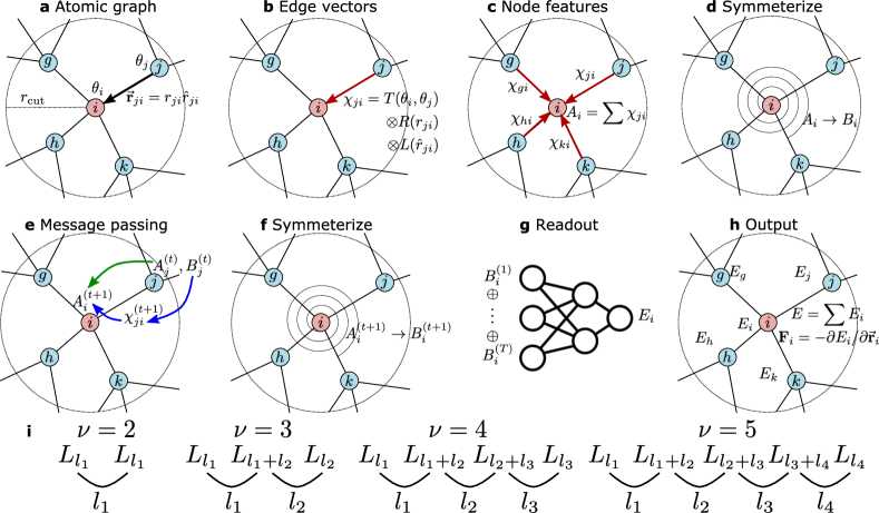
Figure 1: Schematic of the CACE potential. a-h show each step of the operation, and i illustrates the rule for making rotationally invariant features.

For both the sender node and the receiver node of an edge, the elements $\alpha_{i}$ are first mapped to vectors of lengths equal to the total number of elements $N_{\mathrm{element}}$ via one-hot embedding, and then the one-hot vectors are multiplied with a learnable weight matrix of size $N_{\mathrm{embedding}}\times N_{\mathrm{element}}$ outputting a learnable embedding $\boldsymbol{\theta}_{i}$ for each atom $i$ of length $N_{\mathrm{embedding}}$. Typically, $N_{\mathrm{embedding}}$ is selected to be a small number between 1 and 4. This continuous element embedding eliminates the unfavorable scaling of using discrete chemical element types when representing atomic environments, and also allows alchemical learning.

Edge basis

The edge basis, shown in Fig. 1b, is used to describe the spatial arrangement of an atom $j$ around the atom $i$ ($\vec{\mathbf{r}}_{ji}\equiv\mathbf{r}_{j}-\mathbf{r}_{i}$, $r_{ji}=|\vec{\mathbf{r}}_{ji}|$ and $\hat{\mathbf{r}}_{ji}=\vec{\mathbf{r}}_{ji}/r_{ji}$), and is formed by the product of a radial basis $R$, an angular basis $L$, and an edge-type basis $T$:

$$\chi_{cn\mathbf{l}}(\sigma_{i},\sigma_{j})=T_{c}(\sigma_{i},\sigma_{j})R_{n,cl}(r_{ji})L_{\mathbf{l}}(\hat{\mathbf{r}}_{ji}).$$ (1)

Eqn. (1) is general and fundamental for many MLIPs, and a systematic discussion of the design choices for each term can be found in Ref. Batatia et al. (2022b).

In CACE, the type of edge depends on the states of the two nodes it connects. In the initial layer, the edge states are only determined by the chemical elements of the two atoms $i$ and $j$. The edge is encoded using the flattened tensor product of the two node embedding vectors, $\boldsymbol{\theta}_{i}\otimes\boldsymbol{\theta}_{j}$, resulting in an edge feature of length $c=N_{\mathrm{embedding}}^{2}$. In a later message passing layer $t$, the edge features can depend on the node hidden features $\mathbf{h}_{i}^{(t)}$. Such edge encoding formed by the tensor product can be interpreted as the attention mechanism Vaswani et al. (2017) between the two atoms, with the sender and the receiver node embedding vectors being the query and the key.

The orientation-dependent angular basis is

$$L_{\mathbf{l}}(\hat{\mathbf{r}}_{ji})=(x_{j}-x_{i})^{l_{x}}(y_{j}-y_{i})^{l_{y}}(z_{j}-z_{i})^{l_{z}},$$ (2)

where $\mathbf{l}\equiv(l_{x},l_{y},l_{z})$ are the angular momentum numbers satisfying $l_{x}+l_{y}+l_{z}=l$, with $l$ being the total angular momentum. Such angular basis is just spherical harmonic functions in Cartesian basis. Indeed, one can easily transform the function of a certain angular momentum number $l$ in Cartesian and spherical harmonic bases by a simple matrix multiplication Altmann (1957).

$R_{n,cl}(r_{ji})$ is a set of radial basis consisting of $n$ functions, coupled with the total angular momentum $l$ and the edge channel $c$. This means that, for each $l$ and $c$ combination, there is a different set of $n$ radial functions. In CACE, the raw radial embedding block uses a set of trainable Bessel functions with different frequencies Schütt et al. (2021) multiplied by a smooth cutoff function. The output is then mixed using a linear transformation to form $R_{n,cl}$ for each $l$ and $k$.

Atom-centered basis ($A$-basis)

As shown in Fig. 1c, the atom-centered representation is made by summing over all the edges of a node,

$$A_{i,cn\mathbf{l}}=\sum_{j\in\mathcal{N}(i)}\chi_{cn\mathbf{l}}(\sigma_{i},\sigma_{j}).$$ (3)

This corresponds to a projection of the edge basis on the atomic density, which is commonly referred to as the “density trick” and was introduced originally to construct SOAP and bispectrum descriptors Bartók et al. (2013).

Symmetrized basis ($B$-basis)

The orientation-dependent $A$ features are symmetrized to get the invariant $B$ features of different body orders $\nu$ as sketched in Fig. 1c. For $l=0$, $A$ is already rotationally invariant, so the $\nu=1$ features $B^{(1)}_{i,cn0}=A_{i,cn\textbf{0}}$. For $\nu\geq 2$, the general rule for constructing the symmetrized basis is illustrated in Fig. 1i. The key idea is that pairs of angular features need to have a shared factor of $\mathbf{l}$, when summed over to form invariants. If a combination contains any elements satisfying $\mathbf{l}=\mathbf{0}$ or $\mathbf{l}=\mathbf{l^{\prime}}$, the resulting invariant can be constructed using the product of lower-order invariants, and can thus be eliminated for redundancy. Other radial or edge terms that do not depend on $\mathbf{l}$ or only depend on the total angular momentum $l$ can be multiplied on top without breaking the rotational symmetry.

More specifically, for $\nu=2$ Zhang et al. (2021a),

$$B_{i,cnl_{1}}^{(2)}=\sum_{\mathbf{l}_{1}}\mathcal{C}(\mathbf{l}_{1})A_{i,cn\mathbf{l}_{1}}^{2},$$ (4)

summed over all $\mathbf{l}_{1}$ with $l_{1x}+l_{1y}+l_{1z}=l_{1}$. $\mathcal{C}(\mathbf{l})=\dfrac{l!}{l_{x}!l_{y}!l_{z}!}$ is the combinatorial prefactor. Doing the expansion explicitly, one can use the multinomial formula to show that Zhang et al. (2021a)

$$B_{i,cnl_{1}}^{(2)}=\sum_{j,k\in\mathcal{N}(i)}T_{c}(\sigma_{i},\sigma_{j})R_{n,cl}(r_{ji})T_{c}(\sigma_{i},\sigma_{k})R_{n,cl}(r_{ki})\\ \times r_{ji}^{l_{1}}r_{ki}^{l_{1}}cos^{l_{1}}(\theta_{ijk}).$$ (5)

So this term includes three-body contributions of $\vec{\mathbf{r}}_{ji}$ and $\vec{\mathbf{r}}_{ki}$ together with their enclosed angle $\theta_{ijk}$. For $\nu=3$,

$$B_{i,cnl_{1}l_{2}}^{(3)}=\sum_{\mathbf{l}_{1},\mathbf{l}_{2}}\mathcal{C}(\mathbf{l}_{1})\mathcal{C}(\mathbf{l}_{2})A_{i,cn\mathbf{l}_{1}}A_{i,cn(\mathbf{l}_{1}+\mathbf{l}_{2})}A_{i,cn\mathbf{l}_{2}},$$ (6)

which includes four-body interaction terms in the form $r_{ji}^{l_{1}}r_{ki}^{l_{1}+l_{2}}r_{hi}^{l_{2}}cos^{l_{1}}(\theta_{ijk})cos^{l_{2}}(\theta_{ikh})$. For $\nu=4$,

$$B_{i,cnl_{1}l_{2}l_{3}}^{(4)}=\sum_{\mathbf{l}_{1},\mathbf{l}_{2},\mathbf{l}_{3}}\mathcal{C}(\mathbf{l}_{1})\mathcal{C}(\mathbf{l}_{2})\mathcal{C}(\mathbf{l}_{3})\\ \times A_{i,cn\mathbf{l}_{1}}A_{i,cn(\mathbf{l}_{1}+\mathbf{l}_{2})}A_{i,cn(\mathbf{l}_{2}+\mathbf{l}_{3})}A_{i,cn\mathbf{l}_{3}},$$ (7)

which includes five-body contributions in the form $r_{ji}^{l_{1}}r_{ki}^{l_{1}+l_{2}}r_{hi}^{l_{2}+l_{3}}r_{gi}^{l_{3}}cos^{l_{1}}(\theta_{ijk})cos^{l_{2}}(\theta_{ikh})cos^{l_{3}}(\theta_{ihg})$.

Based on the expansion, one can see that these $B^{(\nu)}$ terms are the same as the $B^{(\nu)}$ terms in the original ACE paper Drautz (2019), although the computation in the Cartesian space is much more straightforward. The $B$ basis is a complete basis of permutation and rotation invariant functions of the atomic environment Drautz (2019). In practice, one truncates the series up to some maximum values of $l_{\mathrm{max}}$ and $\nu_{\mathrm{max}}$ to make the computation tractable. The dimension of the $B$ basis is $c\times n\times N_{L}$, where each factor comes from the number of edge channels, radial basis, and angular basis, respectively. Fig. 2 shows the total number of angular features $N_{L}$ up to certain $l_{\mathrm{max}}$ and $\nu_{\mathrm{max}}$. The number of $N_{l}$ is compact even for $\nu_{\mathrm{max}}=5$. For most practical applications, $l_{\mathrm{max}}$ between 2 and 4 and $\nu_{\mathrm{max}}$ between 2 and 4 are sufficient for good accuracy when fitting CACE potentials.

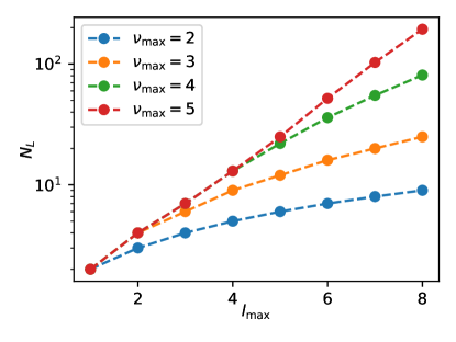
Figure 2: The total number of angular features $N_{L}$, for maximum values of $l_{\mathrm{max}}$ and $\nu_{\mathrm{max}}$.

Message passing

The framework above reproduces the original ACE, albeit formulated entirely in the Cartesian space. In ACE, the atomic energy of each atom is determined by the neighboring atoms within its cutoff radius $r_{\mathrm{cut}}$. On top of that, one can incorporate message passing, which iteratively propagates information along the edges, thereby communicating the local information and effectively enlarging the perceptive field of each atom.

CACE uses two types of message passing (MP) mechanisms. The first type, denoted by the green arrow in Fig. 1e, communicates the $A$ information between neighboring atoms: the orientation-dependent message from atom $j$ to $i$ can be expressed as:

$$m_{1,j\rightarrow i,cn\mathbf{l}}^{(t)}=F_{cnl}(r_{ji})A_{j,cn\mathbf{l}}^{(t)}$$ (8)

where $F_{cnl}(r_{ji})$ is a filter function that takes the scalar value of the distance $r_{ji}$, and it can depend on edge channel, radial channel and total angular momentum. In practice, we use an exponential decay function with trainable exponent, to capture the physics that farther atoms have less effect, although other choices are possible.

The second MP mechanism, denoted by the two blue arrows in Fig. 1e, uses a recursive edge embedding scheme analogous to REANN Zhang et al. (2021a):

$$m_{2,j\rightarrow i,cn\mathbf{l}}^{(t)}=H_{cl}(B_{j}^{(t)})\chi_{cn\mathbf{l}}(\sigma_{i},\sigma_{j}),$$ (9)

where $H_{cl}$ is a trainable scalar function that can optionally depend on edge channel and total angular momentum. We simply use a linear neural network (NN) layer for $H$.

The aggregated message is

$$M_{i,cn\mathbf{l}}^{(t)}=\sum_{j\in\mathcal{N}(i)}m_{1,j\rightarrow i,kn\mathbf{l}}^{(t)}+m_{2,j\rightarrow i,kn\mathbf{l}}^{(t)}$$ (10)

One can then update the $A$ representation of each node,

$$A_{i,cn\mathbf{l}}^{(t+1)}=G(A_{i,cn\mathbf{l}}^{(t)},M_{i,cn\mathbf{l}}^{(t)}),$$ (11)

and for $G$ we use a simple linear function. After obtaining the updated $A^{(t+1)}$, we again take the symmetrized $B$-basis as described before. It is easy to verify that these symmetrized representations are only dependent on the scalar values of the atomic distances and angles, and thus rotationally invariant. Note that one can make various design choices for $F$, $H$ and $G$ functions: they can be dependent on $c$, $n$ and $l$, without breaking the invariance at the symmetrization stage.

In practice, only one or no MP layer is typically used in CACE. This is because the use of higher-body-order atomic features and messages reduces the need for many MP layers, as in the case of MACE Batatia et al. (2022a).

Readout and output

After $T$ MP layers, all the resulting $B$ features at each layer are concatenated. These invariant features are compact; the number of the features can be computed as $T\times c\times n\times N_{L}$. Then, a multilayer perceptron (MLP) maps these invariant features to the target of the atomic energy of each atom $i$,

$$E_{i}=MLP(B_{i}^{(0)}\oplus B_{i}^{(1)}\oplus\ldots\oplus B_{i}^{(T)}).$$ (12)

In practice, for the readout function we use the sum of a linear NN and a multilayer NN, as the former preserves the body-ordered contributions and the latter considers the higher-ordered terms from the truncated series.

Finally, the total potential energy of the system is the sum of all the atomic energies of each atom, and the forces can readily be computed by taking the derivatives of the total energy with respect to atomic coordinates.

III Applications

III.1 Bulk water

As an example application on complex fluids, we demonstrate CACE on a dataset of 1,593 liquid water configurations, each of 64 molecules Cheng et al. (2019). The dataset was computed at the revPBE0-D3 level of density functional theory (DFT). 90% of the data are used in the training. We used a cutoff $r_{\mathrm{cut}}=5.5$ Å, 6 Bessel radial functions and $c=12$, $l_{\mathrm{max}}=3$, $\nu_{\mathrm{max}}=3$, $N_{\mathrm{embedding}}=3$, and no message passing ($T=0$) or one message passing layer ($T=1$). The fitted CACE models have relatively few parameters: 24,572 trainable parameters for the CACE water model with $T=0$, and 69,320 trainable parameters for the model with $T=1$. The root mean square errors (RMSE) of the energy per water molecule and forces on the validation set are presented in Table 1.

Table 1: Root mean square errors (RMSE) for energy (E) per water molecule (in meV/H₂O) and force (in meV/Å) on a liquid water dataset from Ref. Cheng et al. (2019). The cutoffs $r_{\mathrm{cut}}$ of the atomic environment and the numbers of message passing layers are listed.

	BPNN Cheng et al. (2019)	DeepMD Wang et al. (2018)	EANN Zhang et al. (2021b)	linear ACE Witt et al. (2023)	REANN Zhang et al. (2021a)	NequIP Batzner et al. (2022)	MACE Batatia et al. (2022a)	CACE	CACE
	$6.35$ Å	$6$ Å	$6.2$ Å	$5.5$ Å	$6.2$ Å, $T=3$	$4.5$ Å, $T=3$	$6$ Å	$5.5$ Å, $T=0$	$5.5$ Å, $T=1$
E	7.0	6.3	6.3	5.196	2.4	2.8	1.9	3.49	1.77
F	120	92	129	99	53.2	45	36.2	79	47

Table 1 compares the RMSE error of other MLIPs trained on the same dataset. The NequIP and DeepMD models are trained by us, and the others are from the references. In addition, we also trained a MACE model with E RMSE=1.9 meV/H₂O, F RMSE=46.8 meV/Å. as the original Behler-Parrinello neural network (BPNN) in Ref. Cheng et al. (2019) was trained using the RuNNer code Behler (2018), we also trained another one using N2P2 Singraber et al. (2019) and obtained E RMSE=5.8 meV/H₂O, F RMSE=108 meV/Å. MLIPs based on three-body and three-body descriptors without message passing, including BPNN based on ACSFs Behler and Parrinello (2007), embedded atom neural network (EANN) Zhang et al. (2021b), and DeepMD have similar errors, and they are amongst the highest in this comparison. Linear ACE uses higher-body order features, which can be directly compared to the CACE model trained with the same cutoff and without message passing ($r_{\mathrm{cut}}=5.5$ Å, $T=0$), and the latter has lower error. The REANN potential Zhang et al. (2021a) with three message passing layers, the equivariant message passing model NequIP Batzner et al. (2022), the high body order MACE Batatia et al. (2022a) model, and the CACE model with $T=1$ have the lowest errors.

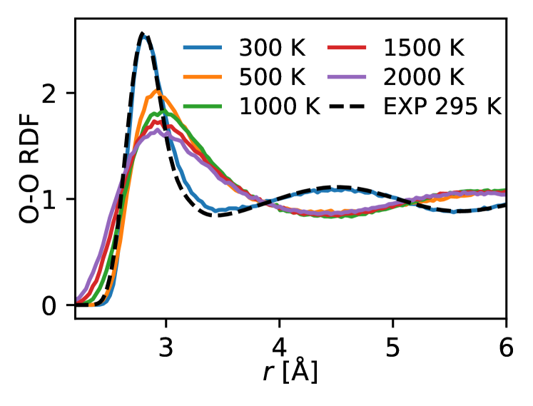
a b

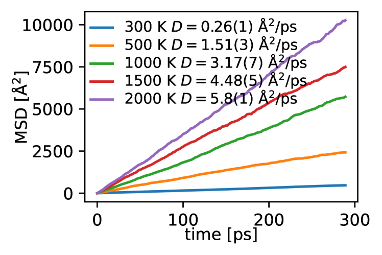
Figure 3: Simulation results of water using CACE $T=1$ model. a Oxygen-oxygen radial distribution functions (RDF) at different temperatures and 1 g/mL computed via classical MD simulations in the NVT ensemble. The experimental O-O RDF at ambient conditions was obtained from Ref Skinner et al. (2014). b Mean squared displacement (MSD) from the liquid water simulations. Diffusivities ($D$) are shown in the legends.

For running molecular dynamics (MD) simulations using MLIPs, besides accuracy, a crucial requirement is the stability - the possibility to run long-enough trajectories with the system remaining in physically reasonable states and the simulation not exploding, even at conditions with few or no training data. To assess the simulation stability, we performed independent simulations of 300 ps in length for water at 1 g/mL at 300 K, 500 K, 1000 K, 1500 K, and 2000 K using the CACE $T=1$ model. The simulation cell contains 512 water molecules. The time step was 1 fs, and Nosé–Hoover thermostat was used. The upper panel of Fig. 3 shows the oxygen-oxygen (O-O) radial distribution function (RDF). At 300 K, the computed O-O RDF is in excellent agreement with experiment from X-ray diffraction measurements Skinner et al. (2014). Note that the nuclear quantum effects have a slight destructuring effect in the O-O RDF, but the effect is quite small Cheng et al. (2019). The mean squared displacements (MSD) from these simulations are shown on the lower panel of Fig. 3. The diffusivity $D$, obtain by fitting a linear function to the MSD, at 300 K agrees well with the DFT MD result ($D_{\mathrm{DFT}}=2.67\pm 0.10\mathrm{\AA}^{2}/$ps) from Ref. Marsalek and Markland (2017). At high temperatures up to 2000 K, the MD simulations remained stable, which demonstrate the superior stability of the CACE potential. Note that we do not expect the result at the very high temperatures to be physically predictive, and this example is just to illustrate the stability of CACE. Such stability is not only necessary for converging statistical properties, but also allows the refinement of the potential: to iteratively improve the accuracy of the potential under certain conditions, one can perform active learning which collects snapshots from corresponding MD trajectories and use these snapshots for re-training.

III.2 Small molecules: ethanol and 3BPA

To demonstrate CACE on small organic molecules, we fitted to the ethanol sampled from DFT molecular dynamics simulations at 500 K, which is from the MD17 database Chmiela et al. (2017) that is often used for benchmark purposes. We used a cutoff $r_{\mathrm{cut}}=4$ Å, 6 Bessel radial functions, $c=12$, $l_{\mathrm{max}}=4$, $\nu_{\mathrm{max}}=3$, $N_{\mathrm{embedding}}=4$, and one message passing layer ($T=1$). The model was trained on 1,000 structures randomly selected from the dataset (90% train/10% validation split), and tested on another 10,000 random structures.

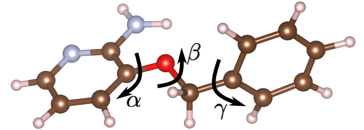
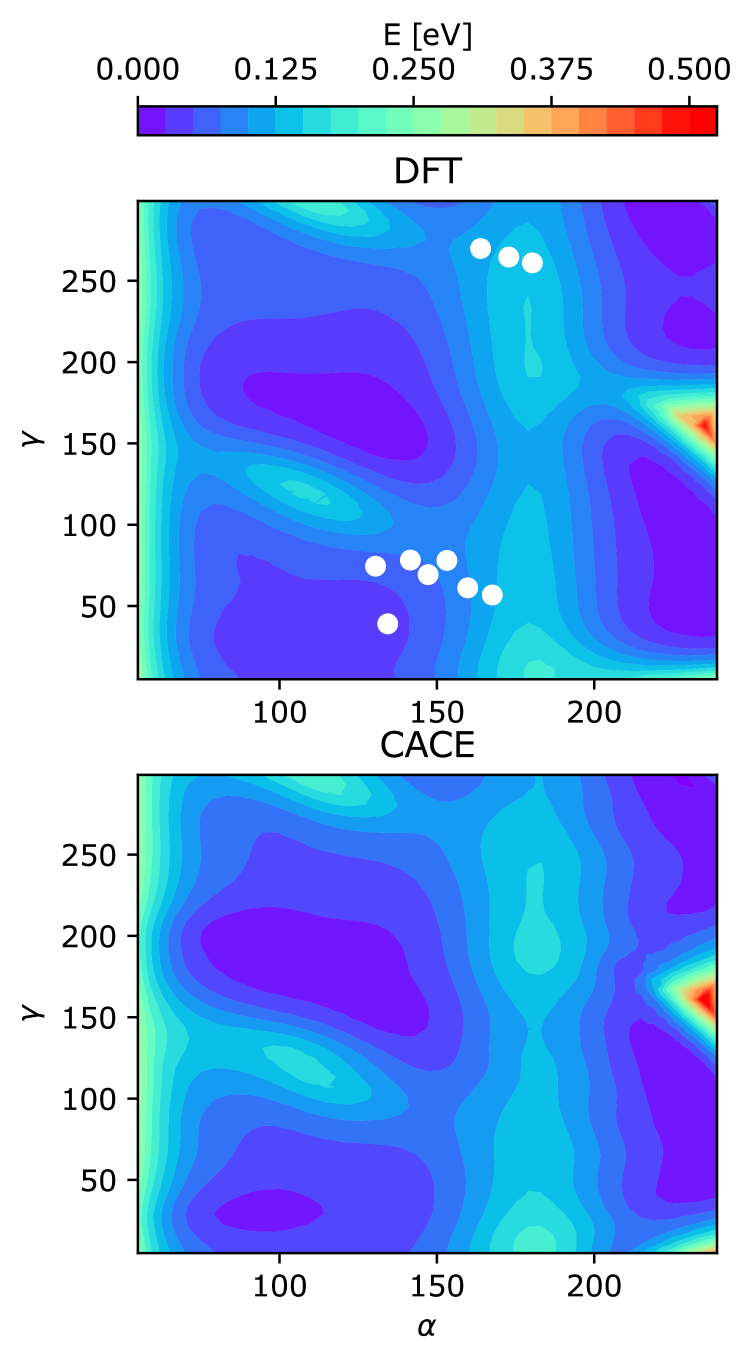
a b

Figure 4: The dihedral scan benchmark of the 3BPA molecule. a Molecular structure and three dihedral angles. b The dihedral potential energy landscape for $\beta=120^{\circ}$, as predicted by DFT and CACE. The white dots on the DFT potential energy surface correspond to all the training configurations that have $\beta$ between 100^∘ and 140^∘.

	SchNet Schütt et al. (2017)	DimeNet Gasteiger et al. (2019)	sGDML Chmiela et al. (2019)	PaiNN Schütt et al. (2021)	SphereNet Liu et al. (2022)	NewtonNet Haghighatlari et al. (2022)	GemNet-T Gasteiger et al. (2021)	NequIP Batzner et al. (2022)	CACE
E	3.5	2.8	3.0	2.7		2.6		2.2	2.37
F	16.9	10.0	14.3	9.7	9.0	9.1	3.7	3.1	7.0
S $\uparrow$	247	26		86	33		169	300	300

Table 2: Mean absolute error (MAE) of energy (E) and force (F) for ethanol in the MD-17 dataset, in units of meV and meV/Å, respectively, trained on 1000 reference configurations. The stability (S) in the unit of ps shows how long the simulation using the MLIP is physically realistic in MD of a maximum length of 300 ps at 500 K. Besides CACE, the errors are obtained from respective references, and the stability is from Ref. Fu et al. (2023).

Table 2 shows a comparison of the different MLIPs trained on energies and forces for the same MD17-ethanol dataset. The energy accuracy of CACE is similar to the NequIP model with $T=5$, although the CACE force error is larger. The stability (S) in Table 2 measures how long MD simulations at 500 K using the MLIP is physically sensical (no pathological behavior or enter physically prohibitive states) in runs with a maximum length of 300 ps, so 300 ps is the maximum score in this case Fu et al. (2023). The stability values for other MLIPs are from Ref. Fu et al. (2023) which used 10,000 training structures and a time step of 0.5 fs in MD. For CACE, we used 1,000 training structures and a time step of 1 fs, which is more stringent, but the MD had nevertheless remained stable. As observed in Refs. Fu et al. (2023); Stocker et al. (2022), force accuracy does not imply stability, and the latter is a key metric for MLIPs.

	ACE Drautz (2019)	sGDML Chmiela et al. (2019)	GAP Bartók et al. (2010)	ANI-pretrained Gao et al. (2020)	ANI-2x Gao et al. (2020)	NequIP Musaelian et al. (2023)	MACE Batatia et al. (2022a)	CACE
300 K, E	7.1	9.1	22.8	23.5	38.6	3.3	3.0	6.3
300 K, F	27.1	46.2	87.3	42.8	84.4	10.8	8.8	21.4
600 K, E	24.0	484.8	61.4	37.8	54.5	11.2	9.7	18.0
600 K, F	64.3	439.2	151.9	71.7	102.8	26.4	21.8	45.2
1200 K, E	85.3	774.5	166.8	76.8	88.8	38.5	29.8	58.0
1200 K, F	187.0	711.1	305.5	129.6	139.6	76.2	62.0	113.8

Table 3: Root mean square errors (RMSE) for energy (E) and force (F) on the 3BPA temperature transferability dataset, reported in units of meV and meV/Å. All models were trained on $T=300$ K data. Results of previous models except for NequIP and MACE are from Kovács et al. (2021). ANI-2x was trained on 8.9 million structures, and ANI-pretrained was pretrained and fine-tuned on this dataset.

As another example, we fitted to the 3BPA (3-(benzyloxy)pyridin-2-amine) dataset Kovács et al. (2021) consisting of 500 training structures at 300 K. Test data are from simulations at 300 K, 600 K, and 1200 K. We used $r_{\mathrm{cut}}=6$ Å, 8 Bessel radial functions, $c=12$, $l_{\mathrm{max}}=4$, $\nu_{\mathrm{max}}=3$, $N_{\mathrm{embedding}}=4$, and $T=1$. Table 3 shows the errors of different potentials when extrapolating to higher temperature. NequIP and MACE perform the best, while CACE is somewhere between them and ACE. We then compared the dihedral potential energy surface of the molecule. Fig. 4 shows the complex energy landscapes of the $\alpha$-$\gamma$ plane predicted by DFT and by CACE, for the case of $\beta=120^{\circ}$, the plane with the fewest training points. Nevertheless, the CACE landscape closely resembles the ground truth and is regular, more so than the other potentials benchmarked in Ref. Kovács et al. (2021) despite those were trained on a more diverse dataset including high temperature configurations.

III.3 25-element high-entropy alloys

High-entropy alloys, which are composed of several metallic elements, have unique mechanical, thermodynamics, and catalytic properties George et al. (2019). They are challenging to model due to the high number of elements involved, for which many MLIPs scale poorly with. Ref. Lopanitsyna et al. (2023) introduced 25 d-block transition metal HEA dataset that contains 25,630 distorted crystalline structures containing 36 or 48 on bcc or fcc lattices. Ref. Lopanitsyna et al. (2023) further performed an alchemical learning (AL) that explicit compresses chemical space, leading to a model that is both interpretable and very stable.

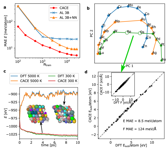
Figure 5: Benchmark on the HEA25 dataset. a Learning curves for different models. Both alchemical learning (AL) models are from Ref. Lopanitsyna et al. (2023). b The first two principal components (PCs) of the CACE embedding matrix. The periods are highlighted with orange, blue, and green lines. Interpolated positions for Re and Os are indicated with empty circles. c Energy comparison between DFT and CACE for a high temperature (5000 K) and a low temperature (300 K) trajectory. The inset shows example solid and melt configurations from the 300 K and the 5000 K trajectories, respectively. d Comparison between the substitution energy $E_{\mathrm{sub}}$, the potential energy difference between the original and the structure substituted with Re and Os element per substitution atom, computed using DFT and CACE. The inset shows the parity plot for the force components computed for those structures.

We took a test set containing 1,000 configurations, and used up to the rest of the 24,630 data points for training and validation. We used $r_{\mathrm{cut}}=4.5$ Å, $l_{\mathrm{max}}=3$, $\nu_{\mathrm{max}}=3$, $T=1$, and $N_{\mathrm{embedding}}=4$ for aggressive alchemical compression.

In Fig. 5a, the CACE learning curve is compared to the ones from Ref. Lopanitsyna et al. (2023), including a 3B model that has an atomic energy baseline and three-body terms, and another 3B+NN model that further incorporates a full set of pair potentials and a non-linear term built on top of contracted power spectrum features. Overall, the CACE model achieved lower error and significantly more efficient learning for fewer data, and it has only 91,232 trainable parameters, compared to more than 160,000 in the 3B+NN model Lopanitsyna et al. (2023).

	AL 3B+NN Lopanitsyna et al. (2023)	PET Pozdnyakov and Ceriotti (2023)	CACE
test, E	10	1.87	5.28
test, F	190	60.1	111
substitute, E	24	N.A.	8.5
substitute, F	373	N.A.	124
5000 K, E	48	152	15.3
5000 K, F	290		233

Table 4: Mean absolute error (MAE) of energy (E) and force (F) for the HEA25 dataset, reported in units of meV and meV/Å. There are three sets of benchmarks on test error, alchemical extrapolation to unseen Re and Os substitute atoms, and temperature transferability to 5000 K.

The errors of the models are presented in Table 4. A very recent architecture, Point Edge Transformer (PET) that utilizes local coordinate systems, achieved state-of-the-art performance in several benchmark systems and also has impressively low test error for the HEA25 dataset Pozdnyakov and Ceriotti (2023). However, as we discuss below, the PET potential has poor transferability.

Alchemical learning capability not only makes learning more efficient, but is also essential towards achieving a foundation model that is valid across the periodic table. CACE is able to perform alchemical learning. The learnable embedding $\boldsymbol{\theta}$ for each element type encodes its chemical information, and can be visualized to gain insights into the data-driven similarities. As the $N_{\mathrm{embedding}}=4$ in this case, we performed a principal component analysis (PCA) and plotted the first two principal component axes in Fig. 5b. The elements are arranged in a way that is strongly reminiscent of their placement in the d-block. This shows that the element embedding scheme is able to learn the nature of the periodic table in a data-driven way.

A stringent way to demonstrate alchemical learning is the extrapolation to unseen elements. In this case, Re and Os are absent from the training set. Ref. Lopanitsyna et al. (2023) provides a hold-out set containing 61 pairs of structures, each of 36 or 48 atoms. Each pair has one fcc or bcc structure with only the original 25 elements, and another structure with up to 11 atoms randomly substituted with Re and Os. We simply took the CACE model trained for the 25-element dataset, and obtained the chemical embedding of Re and Os by a linear interpolation between W and Ir, as illustrated by the empty circles in Fig. 5b. We also added atomic-energy baselines for Re and Os (obtained by fitting the residual energy to a two-parameter linear model that only depends on the Re and Os content). In Fig. 5d we show the parity plot for the substitution energy, defined as the potential energy difference between the original and the substituted structure per substitution atom. Impressively, the CACE error for those substituted structures with unseen elements are rather similar with the test error on the 25-element training set, and is lower than the AL method in Ref. Lopanitsyna et al. (2023). The force comparison, shown in the inset of Fig. 5d, shows the same trend. With the PET potential, it is not clear whether alchemical learning can be performed in a straightforward way.

The most impressive validation of the AL model in Ref. Lopanitsyna et al. (2023) is the extrapolation to configurations very far from the training set: At 5000 K, the systems generated from constant-pressure MD simulations with Monte Carlo element swaps have melted, but the AL potential that was trained exclusively on solid structures is still able to describe the energetics of the structures. This is a test that the PET model Pozdnyakov and Ceriotti (2023) did not perform well. To verify the generalizability of CACE across a wide temperature range, we recomputed the energies and forces of the structures from the 5000 K trajectory as well as another one at a low temperature of 300 K, and show the results in Fig. 5c and Table 4. The CACE errors are a bit smaller compared to Ref. Lopanitsyna et al. (2023), and quite modest compared to the training error.

IV Discussion and limitations

Atomic cluster expansion and equivariant MPNNs are probably both amongst the biggest breakthroughs in the field of MLIPs: the ACE formulation not only guarantees a complete basis for describing atomic environments, but also provides a framework for understanding and connecting different descriptors Drautz (2019); Dusson et al. (2022). E(3) equivariant MPNNs were able to achieve an unprecedented accuracy compared to the previous invariant architectures Batzner et al. (2022); Batatia et al. (2022a). It has been recognized that the spherical harmonics expansion and the subsequent Clebsch-Gordan tensor contraction is a bottleneck in the speed and the simplicity of ACE and these equivariant MPNNs. There have been other approaches that only operates in the Cartesian space, including NewtonNet Haghighatlari et al. (2022), EGNN Satorras et al. (2021), and PaiNN Schütt et al. (2021) that uses atomic displacement vectors in message passing, the PET based on local coordinate systems Pozdnyakov and Ceriotti (2023), and TensorNet that uses Cartesian tensors to represent pairwise displacements Simeon and De Fabritiis (2023). CACE is different from these approaches in that it can be directly mapped to ACE, so like ACE, it is also complete and body-ordered. The completeness helps the accuracy and the smoothness of the potential, particularly when there exists atomic environments that are degenerate using three-body descriptors or bispectrum Pozdnyakov et al. (2020); Nigam et al. (2023). The body order makes the potential more physically interpretable and may help extrapolation. As added advantages, the CACE descriptors are low-dimensional, efficient to evaluate, and are capable of alchemical learning.

A topic that tends to be overlooked in the development of MLIP methods is the stability and generalizability. In practice, a MLIP that is not stable in MD simulations is not useful. Nonetheless, stability and generalization are rarely considered in benchmarks, maybe due to that they are less straightforward to assess than energy and force errors. On the other hand, it has been shown that accuracy of the potential does not imply stability Fu et al. (2023); Stocker et al. (2022). The CACE potential shows high stability and extrapolatability in the datasets we benchmarked: stable MD simulations of water up to 2000 K, MD of ethanol, extrapolation to high temperature and dihedral scan of 3BPA, as well as generalization to the melt and unseen elements in high-entropy alloys. For water, the accuracy of CACE is on par with the most accurate potentials to date, NequIP Batzner et al. (2022) and MACE Batatia et al. (2022a). For small molecules, CACE is less accurate than NequIP or MACE but more accurate than the other recent MLIPs that we compared to. For all practical purposes, the accuracy of CACE for the small molecules is probably enough, considering the error is very small in absolute terms and is way below the chemical accuracy. Moreover, CACE achieved such accuracy with only one message passing layer and relatively few training parameters, and its accuracy can probably be improved with more message passing layers, higher $N_{\mathrm{embedding}}$, $\nu_{\mathrm{max}}$, $l_{\mathrm{max}}$, or a larger MLP at the readout.

We implemented the CACE potential using PyTorch, and the code is available in https://github.com/BingqingCheng/cace. With the current implementation, the training time of the water and the HEA25 datasets took about two days on a vintage GeForce GTX 1080 Ti GPU card, and the small molecules can be trained on a laptop within one or two days. The training should be much faster on state-of-the-art GPUs. For MD simulations of liquid water using the $T=1$ CACE water model on a Nvidia A100 GPU, systems with 1,536 atoms, 5,184 atoms, 12,288 atoms can run 24 ps per hour, 8 ps per hour, 3.5 ps per hour, respectively. The implementation of the code can be further optimized: The computation of the node features and the symmetrization step may be compiled and be made faster. The training and the prediction are available on one GPU and can be made more parallelizable. The MD simulations can be performed in the ASE package, but the LAMMPS interface implementation is currently absent. As CACE has a moderate receptive field, so it is in principle possible to make it scale well in MD simulations.

Many engineering aspects of the CACE potential can be further fine-tuned. For example, dataset normalization and internal normalization can have a large effect on training efficiency and outcome Batatia et al. (2022b). Radial basis influences the learning efficiency Bigi et al. (2022), and its best choice is still an open question. Other choices of $F$, $H$ and $G$ functions in the message passing may be used. The training protocol can also influence the outcome.

Other possible future improvements of CACE include pretraining on large datasets before fine-tuning the model. It should be possible to make a foundation model that is generally valid across the periodic table Batatia et al. (2023). The alchemical learning capability of CACE may facilitate this.

V Conclusions

In summary, we propose a new scheme to preserve the rotational symmetry of atomic environments with different body orders, and the operation is entirely in the Cartesian coordinates. As the transformation to the spherical harmonic basis and the usage of high-dimensional Clebsch-Gordan coupling matrix are avoided, the computation can be more efficient. As the symmetrization in the Cartesian coordinates is equivalent to the Clebsch-Gordan contraction, the scheme can be applied in other MLIPs that use the ACE framework (e.g. linear ACE Witt et al. (2023), SNAP, SOAP-GAP Bartók et al. (2010), Jacobi-Legendre cluster expansion Domina et al. (2023), ml-ACE Bochkarev et al. (2022),), or E(3) equivariant message passing neural networks (e.g. NequIP Batzner et al. (2022), MACE Batatia et al. (2022a), BOTNet Batatia et al. (2022b), SEGNN Brandstetter et al. (2021), Allegro Musaelian et al. (2023)).

Data availability The water dataset is from from https://github.com/BingqingCheng/ab-initio-thermodynamics-of-water. MD17-ethanol is from http://www.sgdml.org/#datasets. BPA is from Ref. Kovács et al. (2021), downloaded from https://github.com/davkovacs/BOTNet-datasets. The HEA25 dataset is from Ref. Lopanitsyna et al. (2023), downloaded from  https://archive.materialscloud.org/record/2023.57.

The training scripts, trained CACE potentials, and MD input files are available at https://github.com/BingqingCheng/cacefit

Code availability The CACE package is publicly available at https://github.com/BingqingCheng/cace.

References

- Keith et al. (2021) John A Keith, Valentin Vassilev-Galindo, Bingqing Cheng, Stefan Chmiela, Michael Gastegger, Klaus-Robert Müller, and Alexandre Tkatchenko, “Combining machine learning and computational chemistry for predictive insights into chemical systems,” Chemical reviews 121, 9816–9872 (2021).
- Unke et al. (2021) Oliver T Unke, Stefan Chmiela, Huziel E Sauceda, Michael Gastegger, Igor Poltavsky, Kristof T Schütt, Alexandre Tkatchenko, and Klaus-Robert Müller, “Machine learning force fields,” Chemical Reviews 121, 10142–10186 (2021).
- Musil et al. (2021) Felix Musil, Andrea Grisafi, Albert P Bartók, Christoph Ortner, Gábor Csányi, and Michele Ceriotti, “Physics-inspired structural representations for molecules and materials,” Chemical Reviews 121, 9759–9815 (2021).
- Drautz (2019) Ralf Drautz, “Atomic cluster expansion for accurate and transferable interatomic potentials,” Physical Review B 99, 014104 (2019).
- Behler and Parrinello (2007) Jörg Behler and Michele Parrinello, “Generalized neural-network representation of high-dimensional potential-energy surfaces,” Physical review letters 98, 146401 (2007).
- Bartók et al. (2010) Albert P Bartók, Mike C Payne, Risi Kondor, and Gábor Csányi, “Gaussian approximation potentials: The accuracy of quantum mechanics, without the electrons,” Physical review letters 104, 136403 (2010).
- Shapeev (2016) Alexander V Shapeev, “Moment tensor potentials: A class of systematically improvable interatomic potentials,” Multiscale Modeling & Simulation 14, 1153–1173 (2016).
- Bartók et al. (2013) Albert P Bartók, Risi Kondor, and Gábor Csányi, “On representing chemical environments,” Physical Review B 87, 184115 (2013).
- Schütt et al. (2017) Kristof Schütt, Pieter-Jan Kindermans, Huziel Enoc Sauceda Felix, Stefan Chmiela, Alexandre Tkatchenko, and Klaus-Robert Müller, “Schnet: A continuous-filter convolutional neural network for modeling quantum interactions,” Advances in neural information processing systems 30 (2017).
- Unke and Meuwly (2019) Oliver T Unke and Markus Meuwly, “Physnet: A neural network for predicting energies, forces, dipole moments, and partial charges,” Journal of chemical theory and computation 15, 3678–3693 (2019).
- Liu et al. (2022) Yi Liu, Limei Wang, Meng Liu, Yuchao Lin, Xuan Zhang, Bora Oztekin, and Shuiwang Ji, “Spherical message passing for 3d molecular graphs,” in International Conference on Learning Representations (ICLR) (2022).
- Gasteiger et al. (2021) Johannes Gasteiger, Florian Becker, and Stephan Günnemann, “Gemnet: Universal directional graph neural networks for molecules,” Advances in Neural Information Processing Systems 34, 6790–6802 (2021).
- Haghighatlari et al. (2022) Mojtaba Haghighatlari, Jie Li, Xingyi Guan, Oufan Zhang, Akshaya Das, Christopher J Stein, Farnaz Heidar-Zadeh, Meili Liu, Martin Head-Gordon, Luke Bertels, et al., “Newtonnet: A newtonian message passing network for deep learning of interatomic potentials and forces,” Digital Discovery 1, 333–343 (2022).
- Satorras et al. (2021) Vıctor Garcia Satorras, Emiel Hoogeboom, and Max Welling, “E (n) equivariant graph neural networks,” in International conference on machine learning (PMLR, 2021) pp. 9323–9332.
- Schütt et al. (2021) Kristof Schütt, Oliver Unke, and Michael Gastegger, “Equivariant message passing for the prediction of tensorial properties and molecular spectra,” in International Conference on Machine Learning (PMLR, 2021) pp. 9377–9388.
- Anderson et al. (2019) Brandon Anderson, Truong Son Hy, and Risi Kondor, “Cormorant: Covariant molecular neural networks,” Advances in neural information processing systems 32 (2019).
- Batzner et al. (2022) Simon Batzner, Albert Musaelian, Lixin Sun, Mario Geiger, Jonathan P Mailoa, Mordechai Kornbluth, Nicola Molinari, Tess E Smidt, and Boris Kozinsky, “E (3)-equivariant graph neural networks for data-efficient and accurate interatomic potentials,” Nature communications 13, 2453 (2022).
- Batatia et al. (2022a) Ilyes Batatia, David P Kovacs, Gregor Simm, Christoph Ortner, and Gábor Csányi, “Mace: Higher order equivariant message passing neural networks for fast and accurate force fields,” Advances in Neural Information Processing Systems 35, 11423–11436 (2022a).
- Geiger and Smidt (2022) Mario Geiger and Tess Smidt, “e3nn: Euclidean neural networks,” arXiv preprint arXiv:2207.09453 (2022).
- Goodman and Wallach (2000) Roe Goodman and Nolan R Wallach, Representations and invariants of the classical groups (Cambridge University Press, 2000).
- Darby et al. (2023) James P Darby, Dávid P Kovács, Ilyes Batatia, Miguel A Caro, Gus LW Hart, Christoph Ortner, and Gábor Csányi, “Tensor-reduced atomic density representations,” Physical Review Letters 131, 028001 (2023).
- Nigam et al. (2020) Jigyasa Nigam, Sergey Pozdnyakov, and Michele Ceriotti, “Recursive evaluation and iterative contraction of n-body equivariant features,” The Journal of Chemical Physics 153 (2020).
- Dusson et al. (2022) Genevieve Dusson, Markus Bachmayr, Gábor Csányi, Ralf Drautz, Simon Etter, Cas van der Oord, and Christoph Ortner, “Atomic cluster expansion: Completeness, efficiency and stability,” Journal of Computational Physics 454, 110946 (2022).
- Batatia et al. (2022b) Ilyes Batatia, Simon Batzner, Dávid Péter Kovács, Albert Musaelian, Gregor NC Simm, Ralf Drautz, Christoph Ortner, Boris Kozinsky, and Gábor Csányi, “The design space of e (3)-equivariant atom-centered interatomic potentials,” arXiv preprint arXiv:2205.06643 (2022b).
- Vaswani et al. (2017) Ashish Vaswani, Noam Shazeer, Niki Parmar, Jakob Uszkoreit, Llion Jones, Aidan N Gomez, Łukasz Kaiser, and Illia Polosukhin, “Attention is all you need,” Advances in neural information processing systems 30 (2017).
- Altmann (1957) SL Altmann, “On the symmetries of spherical harmonics,” in Mathematical Proceedings of the Cambridge Philosophical Society, Vol. 53 (Cambridge University Press, 1957) pp. 343–367.
- Zhang et al. (2021a) Yaolong Zhang, Junfan Xia, and Bin Jiang, “Physically motivated recursively embedded atom neural networks: Incorporating local completeness and nonlocality,” Physical Review Letters 127 (2021a), 10.1103/physrevlett.127.156002.
- Cheng et al. (2019) Bingqing Cheng, Edgar A Engel, Jörg Behler, Christoph Dellago, and Michele Ceriotti, “Ab initio thermodynamics of liquid and solid water,” Proceedings of the National Academy of Sciences 116, 1110–1115 (2019).
- Wang et al. (2018) Han Wang, Linfeng Zhang, Jiequn Han, and E Weinan, “Deepmd-kit: A deep learning package for many-body potential energy representation and molecular dynamics,” Computer Physics Communications 228, 178–184 (2018).
- Zhang et al. (2021b) Yaolong Zhang, Ce Hu, and Bin Jiang, “Accelerating atomistic simulations with piecewise machine-learned ab initio potentials at a classical force field-like cost,” Physical Chemistry Chemical Physics 23, 1815–1821 (2021b).
- Witt et al. (2023) William C Witt, Cas van der Oord, Elena Gelžinytė, Teemu Järvinen, Andres Ross, James P Darby, Cheuk Hin Ho, William J Baldwin, Matthias Sachs, James Kermode, et al., “Acepotentials. jl: A julia implementation of the atomic cluster expansion,” The Journal of Chemical Physics 159 (2023).
- Behler (2018) Jörg Behler, RuNNer – A Neural Network Code for High-Dimensional Neural Network Potentials (Universität Göttingen, 2018).
- Singraber et al. (2019) Andreas Singraber, Tobias Morawietz, Jörg Behler, and Christoph Dellago, “Parallel multistream training of high-dimensional neural network potentials,” Journal of chemical theory and computation 15, 3075–3092 (2019).
- Skinner et al. (2014) Lawrie B Skinner, CJ Benmore, Joerg C Neuefeind, and John B Parise, “The structure of water around the compressibility minimum,” The Journal of chemical physics 141, 214507 (2014).
- Marsalek and Markland (2017) Ondrej Marsalek and Thomas E Markland, “Quantum dynamics and spectroscopy of ab initio liquid water: The interplay of nuclear and electronic quantum effects,” The journal of physical chemistry letters 8, 1545–1551 (2017).
- Chmiela et al. (2017) Stefan Chmiela, Alexandre Tkatchenko, Huziel E Sauceda, Igor Poltavsky, Kristof T Schütt, and Klaus-Robert Müller, “Machine learning of accurate energy-conserving molecular force fields,” Science advances 3, e1603015 (2017).
- Gasteiger et al. (2019) Johannes Gasteiger, Janek Groß, and Stephan Günnemann, “Directional message passing for molecular graphs,” in International Conference on Learning Representations (2019).
- Chmiela et al. (2019) Stefan Chmiela, Huziel E Sauceda, Igor Poltavsky, Klaus-Robert Müller, and Alexandre Tkatchenko, “sgdml: Constructing accurate and data efficient molecular force fields using machine learning,” Computer Physics Communications 240, 38–45 (2019).
- Fu et al. (2023) Xiang Fu, Zhenghao Wu, Wujie Wang, Tian Xie, Sinan Keten, Rafael Gomez-Bombarelli, and Tommi S Jaakkola, “Forces are not enough: Benchmark and critical evaluation for machine learning force fields with molecular simulations,” Transactions on Machine Learning Research (2023).
- Stocker et al. (2022) Sina Stocker, Johannes Gasteiger, Florian Becker, Stephan Günnemann, and Johannes T Margraf, “How robust are modern graph neural network potentials in long and hot molecular dynamics simulations?” Machine Learning: Science and Technology 3, 045010 (2022).
- Gao et al. (2020) Xiang Gao, Farhad Ramezanghorbani, Olexandr Isayev, Justin S Smith, and Adrian E Roitberg, “Torchani: A free and open source pytorch-based deep learning implementation of the ani neural network potentials,” Journal of chemical information and modeling 60, 3408–3415 (2020).
- Musaelian et al. (2023) Albert Musaelian, Simon Batzner, Anders Johansson, Lixin Sun, Cameron J Owen, Mordechai Kornbluth, and Boris Kozinsky, “Learning local equivariant representations for large-scale atomistic dynamics,” Nature Communications 14, 579 (2023).
- Kovács et al. (2021) Dávid Péter Kovács, Cas van der Oord, Jiri Kucera, Alice EA Allen, Daniel J Cole, Christoph Ortner, and Gábor Csányi, “Linear atomic cluster expansion force fields for organic molecules: beyond rmse,” Journal of chemical theory and computation 17, 7696–7711 (2021).
- George et al. (2019) Easo P George, Dierk Raabe, and Robert O Ritchie, “High-entropy alloys,” Nature reviews materials 4, 515–534 (2019).
- Lopanitsyna et al. (2023) Nataliya Lopanitsyna, Guillaume Fraux, Maximilian A Springer, Sandip De, and Michele Ceriotti, “Modeling high-entropy transition metal alloys with alchemical compression,” Physical Review Materials 7, 045802 (2023).
- Pozdnyakov and Ceriotti (2023) Sergey N Pozdnyakov and Michele Ceriotti, “Smooth, exact rotational symmetrization for deep learning on point clouds,” arXiv preprint arXiv:2305.19302 (2023).
- Simeon and De Fabritiis (2023) Guillem Simeon and Gianni De Fabritiis, “Tensornet: Cartesian tensor representations for efficient learning of molecular potentials,” arXiv preprint arXiv:2306.06482 (2023).
- Pozdnyakov et al. (2020) Sergey N Pozdnyakov, Michael J Willatt, Albert P Bartók, Christoph Ortner, Gábor Csányi, and Michele Ceriotti, “Incompleteness of atomic structure representations,” Physical Review Letters 125, 166001 (2020).
- Nigam et al. (2023) Jigyasa Nigam, Sergey N Pozdnyakov, Kevin K Huguenin-Dumittan, and Michele Ceriotti, “Completeness of atomic structure representations,” arXiv preprint arXiv:2302.14770 (2023).
- Bigi et al. (2022) Filippo Bigi, Kevin K Huguenin-Dumittan, Michele Ceriotti, and David E Manolopoulos, “A smooth basis for atomistic machine learning,” The Journal of Chemical Physics 157 (2022).
- Batatia et al. (2023) Ilyes Batatia, Philipp Benner, Yuan Chiang, Alin M Elena, Dávid P Kovács, Janosh Riebesell, Xavier R Advincula, Mark Asta, William J Baldwin, Noam Bernstein, et al., “A foundation model for atomistic materials chemistry,” arXiv preprint arXiv:2401.00096 (2023).
- Domina et al. (2023) M Domina, U Patil, M Cobelli, and S Sanvito, “Cluster expansion constructed over jacobi-legendre polynomials for accurate force fields,” Physical Review B 108, 094102 (2023).
- Bochkarev et al. (2022) Anton Bochkarev, Yury Lysogorskiy, Christoph Ortner, Gábor Csányi, and Ralf Drautz, “Multilayer atomic cluster expansion for semilocal interactions,” Physical Review Research 4, L042019 (2022).
- Brandstetter et al. (2021) Johannes Brandstetter, Rob Hesselink, Elise van der Pol, Erik J Bekkers, and Max Welling, “Geometric and physical quantities improve e (3) equivariant message passing,” in International Conference on Learning Representations (2021).