Machine learning mapping of lattice correlated data

Abstract

We discuss a novel approach based on machine learning (ML) regression models to reduce the computational cost of disconnected diagrams in lattice QCD calculations. This method creates a mapping between the results of fermionic loops computed at different quark masses and flow times. The ML model, trained with just a small fraction of the complete data set, provides similar predictions and uncertainties over the calculation done over the whole ensemble, resulting in a significant computational gain.

[1]organization=Institute for Advanced Simulation (IAS-4) - Forschungszentrum Jülich, addressline=Wilhelm-Johnen-Straße, city=Jülich, postcode=52428, country=Germany

[2]organization=Jülich Supercomputing Centre (JSC) & Center for Advanced Simulation and Analytics (CASA), addressline=Wilhelm-Johnen-Straße, city=Jülich, postcode=52428, country=Germany

[3]organization=Institute for Theoretical Particle Physics and Cosmology, TTK, RWTH Aachen University, addressline=Sommerfeldstr. 16, city=Aachen, postcode=52074, country=Germany

[4]organization=Nuclear Science Division, Lawrence Berkeley National Laboratory, city=Berkeley, postcode=CA 94720, country=USA

[5]organization=Department of Physics, University of California, city=Berkeley, postcode=CA 94720, country=USA

1 Introduction

One of the computational challenges in lattice QCD calculations lies in the determination of the quark propagator, which not only serves as the foundation for calculating any fermionic correlation function but is also required in generating gauge ensembles with dynamical quarks. Computing the quark propagator involves inverting a very large sparse matrix representing the lattice Dirac operator. Fermionic disconnected diagrams appear in most hadron matrix element calculations, as well as studies of flavor singlet channels, and standard methods for their calculation are based on stochastic estimates, which are usually computationally expensive.

In this work, we aim to leverage recent developments in Machine Learning (ML) algorithms [1, 2, 3, 4, 5] to expedite the calculation of fermionic disconnected diagrams in lattice QCD. When calculating such diagrams lots of data are generated depending on the number of stochastic sources and gauge configurations used. Translational invariance can be used to improve the signal-to-noise ratio, providing additional data. We have defined both the training and the bias-correction sets taking advantage of the large number of stochastic sources and translational invariance. ML algorithms have been already applied in Ref. [6] to try to reconstruct the Euclidean time dependence of more complicated observables training a ML mapping based on the correlation with simpler observables. We have investigated the possibility to train a ML mapping to relate fermionic disconnected diagrams evaluated at different parameters, such as quark masses or flow times.

The gradient flow [7, 8] provides a favorable regulator of short-distance singularities due to its reduced operator mixing, essentially trading power divergent lattice spacing effects with a milder finite $1/t$ dependence. By keeping the flow time $t$ fixed, one can then perform the continuum limit with no renormalization ambiguities. An example of the advantage of the use of the Gradient Flow is the simplified calculation of the quark content of nucleons [9, 10]. The application of the gradient flow to the calculation of fermionic disconnected diagrams is beneficial both to simplify the renormalization and to improve the signal-to-noise ratio.

In Sec. 2 we describe the stochastic method we use to determine the fermionic disconnected diagrams. In Sec. 3 we study the correlation between data and, in Sec. 4 we describe the algorithm and present our results.

2 Fermionic disconnected diagrams

We consider a lattice of spacing $a$ and box size $V=L^{3}\times T$, with Dirac fermions in the fundamental representation of SU($N_{\text{c}}=3$), $\psi_{a,\alpha},\overline{\psi}_{a,\alpha}$ ($a=1,\ldots,N_{\text{c}}=3$ and $\alpha=1,\ldots,4$). We adopt periodic boundary conditions for all fields, excluding fermion fields taken to be anti-periodic in Euclidean time. These boundary conditions preserve translational invariance. In lattice QCD, the calculation of physical observables involving fermions, requires the determination of the quark propagators, $\left[\psi_{a,\alpha}(x)\overline{\psi}_{b,\beta}(y)\right]_{\text{F}}=S^{ab}_{\alpha\beta}(x,y)$, where with $\left[\cdot\right]_{\text{F}}$ we indicate a fermionic contraction. For simple correlation functions, like the kaon or the nucleon 2-point functions, one requires only the calculation of one column of the inverse, $S$, of the lattice Dirac operator, $D$,

$$D^{ab}_{\alpha\beta}(x,y)S^{bc_{0}}_{\beta\gamma_{0}}(y,z_{0})=\frac{1}{a^{4}}\delta_{ac_{0}}\delta_{\alpha\gamma_{0}}\delta_{xz_{0}}\,,$$ (1)

where the source location, $z_{0}$, and the corresponding spin and color indices, $\gamma_{0}$ and $c_{0}$, are fixed. Repeated indices, $\beta$, $b$, and $y$ in this case, are summed over. To determine all-to-all propagators, where the source location is not fixed, or to calculate quantities related to all-to-all propagators, like the trace of the quark propagator, we have to rely on stochastic methods.

To calculate the all-to-all propagator one takes a set of $r=1,\ldots,N_{\eta}$ of complex random vectors $\eta^{(r)}_{a\alpha}(x)$ that satisfy

$$\lim_{N_{\eta}\rightarrow\infty}\left\langle\eta_{a\alpha}(x)\eta_{b\beta}(y)^{*}\right\rangle_{\eta}=\delta_{ab}\delta_{\alpha\beta}\delta_{xy}\,,$$ (2)

where with $\left\langle\cdot\right\rangle_{\eta}$ we indicate the average over $N_{\eta}$ stochastic vectors

$$\left\langle\eta_{a\alpha}(x)\eta_{b\beta}(y)^{*}\right\rangle_{\eta}=\frac{1}{N_{\eta}}\sum_{r=1}^{N_{\eta}}\eta_{a\alpha}^{(r)}(x)\eta_{b\beta}^{(r)*}(y)\,.$$ (3)

To estimate the all-to-all propagator one can now solve

$$D^{ab}_{\alpha\beta}(x,y)\phi_{b\beta}(y)=\frac{1}{a^{4}}\eta_{a\alpha}(x)\,.$$ (4)

The full propagator is then reconstructed by the unbiased estimator

$$S^{ab}_{\alpha\beta}(x,y)=\lim_{N_{\eta}\rightarrow\infty}\left\langle\phi_{a\alpha}(x)\eta_{b\beta}(y)^{*}\right\rangle_{\eta}\,,$$ (5)

up to noise contributions at finite $N_{\eta}$. The noise of the estimator is of the order of O($\sqrt{12V/N_{\eta}}$) and one needs variance reduction techniques to reach a signal-to-noise ratio of O($1$). One example of variance reduction would be the use of time-dilution [11]. Another choice is to use the one-end trick [12] and the generalization called linked stochastic sources [13] where the stochastic vector is non-vanishing only for specific color, spin or space-time indices. We denote linked stochastic sources with $\eta^{(b,\beta)}_{a\alpha}(x)$ where the color and Dirac indices $b$ and $\beta$ are fixed

$$\eta^{(b,\beta)}_{a\alpha}(x)=\delta_{ab}\delta_{\alpha\beta}\eta_{a\alpha}(x)\,.$$ (6)

We now solve for all the fixed couple of values $(a_{0},\alpha_{0})$

$$D^{ab}_{\alpha\beta}(x,y)\phi^{(a_{0}\alpha_{0})}_{b\beta}(y)=\frac{1}{a^{4}}\eta^{(a_{0}\alpha_{0})}_{a\alpha}(x)\,.$$ (7)

For different quark flavors, $f=\ell,s$, one obtains different solutions $\phi^{f}(y)$. To not clutter the notation, we leave the flavor index unspecified when discussing the generalities of the quark propagator determination. The quantity of interest is the quark propagator, $S^{a_{0}b_{0}}_{\alpha_{0}\beta_{0}}(x,y)$ that can be determined for each gauge configuration up to noise contributions by

$$\left[\psi^{a_{0}}_{\alpha_{0}}(x)\overline{\psi}^{b_{0}}_{\beta_{0}}(y)\right]_{\text{F}}=S^{a_{0}b_{0}}_{\alpha_{0}\beta_{0}}(x,y)=\left\langle\eta^{(a_{0},\alpha_{0})}_{c\gamma}(x)^{*}\phi^{(b_{0}\beta_{0})}_{c\gamma}(y)\right\rangle_{\eta}\,.$$ (8)

Reintroducing a flavor index, the quark condensates at vanishing flow times is denoted by

$$\left\langle\overline{\psi}_{f}\psi_{f}\right\rangle=\frac{a}{T}\sum_{x_{4}}\left\langle C^{f}_{\overline{\psi}\psi}(x_{4};\eta,U)\right\rangle_{\text{G},\eta}\,,$$ (9)

where $\left\langle\cdot\right\rangle_{\text{G},\eta}$ denotes the average over the gauge ensemble and the stochastic sources. $C^{f}_{\overline{\psi}\psi}(x_{4};\eta,U)$ is evaluated on a fixed gauge background, $U(x,\mu)$, and on a given stochastic source, $\eta(x)$

$$C^{f}_{\overline{\psi}\psi}(x_{4};\eta,U)=-\frac{a^{3}}{L^{3}}\sum_{{\bf x}}\sum_{a_{0},\alpha_{0}}\eta^{(a_{0},\alpha_{0})}_{c\gamma}({\bf x},x_{4})^{*}\phi^{f,(a_{0}\alpha_{0})}_{c\gamma}({\bf x},x_{4})\,,\qquad f=\ell,~{}s\,.$$ (10)

The specific choice of the stochastic vector $\eta(x)$ is not critical as far as the condition (3) is satisfied and the variance is under control. For a complex matrix like $D^{ab}_{\alpha\beta}(x,y)$ a standard choice is to use stochastic vectors belonging to $\mathbbm{Z}_{4}$, i.e for each $a,\alpha,x$ the vector $\eta_{a\alpha}(x)$ takes one of the values $\{\pm 1,\pm i\}$ with the same probability (see Ref. [14] and refs. therein for a discussion on the choice of stochastic vectors and variance reduction techniques).

We also studied the flowed scalar quark condensate

$$\left\langle\overline{\chi}_{f}\chi_{f}\right\rangle=\frac{a}{T}\sum_{x_{4}}\left\langle C^{f}_{\overline{\chi}\chi}(x_{4},t;\eta,U)\right\rangle_{\text{G},\eta}$$ (11)

where

$$C_{\overline{\chi}\chi}(x_{4},t;\eta,U)=\frac{a^{3}}{L^{3}}\sum_{{\bf x}}\sum_{a,\alpha}\left[\overline{\chi}^{a}_{\alpha}({\bf x},x_{4},t)\chi^{a}_{\alpha}({\bf x},x_{4},t)\right]_{\text{F}}\,.$$ (12)

The fermion fields $\chi(x,t)$ and $\overline{\chi}(x,t)$ satisfy the gradient flow equations of Refs. [7, 8], but the results of this work do not depend on the particular choice of gradient flow equations.

The first step is to solve for each pair $(a_{0},\alpha_{0})$ the equation

$$D^{ab}_{\alpha\beta}(x,y)\phi^{(a_{0}\alpha_{0})}_{b\beta}(y;0,t)=\frac{1}{a^{4}}\xi^{(a_{0}\alpha_{0})}_{a\alpha}(x;t,0)\,,$$ (13)

where the source

$$\xi^{(a_{0}\alpha_{0})}_{a\alpha}(x;t,0)=a^{4}\sum_{u}K(u,x;t,0)^{\dagger}\eta^{(a_{0}\alpha_{0})}_{a\alpha}(u)$$ (14)

has to be determined for each value of the flow time $t$ solving the adjoint flow equation

$$\left(\partial_{s}+\Delta\right)\xi^{(a_{0}\alpha_{0})}_{a\alpha}(x;t,s)=0\,,\quad\xi^{(a_{0}\alpha_{0})}_{a\alpha}(x;t,t)=\eta^{(a_{0}\alpha_{0})}_{a\alpha}(x)\,,$$ (15)

to $s=0$. The stochastic vector $\eta^{(a_{0}\alpha_{0})}_{a\alpha}(x)$ is the linked vector adopted in the $t=0$ case defined in Eq. (6). The flowed scalar condensate can then be determined on a single gauge configuration by the expression

$$C^{f}_{\overline{\chi}\chi}(x_{4},t;\eta,U)=-\frac{a^{3}}{L^{3}}\sum_{{\bf x}}\sum_{a_{0},\alpha_{0}}a^{4}\sum_{y}K(x,y;t,0)\phi^{(a_{0}\alpha_{0})}_{c\gamma}(y;0,t)\eta^{(a_{0},\alpha_{0})}_{c\gamma}(x)^{*}\,,$$ (16)

where to compute

$$\phi^{(a_{0}\alpha_{0})}_{c\gamma}(x;t,t)=a^{4}\sum_{y}K(x,y;t,0)\phi^{(a_{0}\alpha_{0})}_{c\gamma}(y;0,t)\,,$$ (17)

is sufficient to solve the gradient flow equation

$$\left(\partial_{t}-\Delta\right)\phi^{(a_{0}\alpha_{0})}_{c\gamma}(x;t,t)=0\,,$$ (18)

where the initial condition is given by the solution of Eq. (13).

We have studied the dependence of the signal-to-noise ratio (SNR) of the scalar condensate on the number of stochastic sources, $N_{\eta}$, for $t/a^{2}=0$ and $t/a^{2}=0.5,~{}0.7$ as representative positive flow times, and the full set of gauge configurations available in the ensembles labeled $M_{1}$ and $M_{3}$ (see Table 1 in the next section). We have not tried to optimize the number of sources, and we choose $N_{\eta}=20$ for all our calculations. Even though this might not be the optimal choice, it is sufficient to test the ML algorithm we propose in this work. It is worth noting that our numerical experiments indicate that a different number of stochastic sources would be needed to saturate the SNR for $t>0$, as a result of the smoothing effect of the gradient flow.

3 Correlation maps and translation invariance

For our numerical experiment we consider the lattice ensembles summarized in Table 1.

Label	$\beta$	$\kappa_{\ell}$	$\kappa_{s}$	$L/a$	$T/a$	${\textrm{c}}_{\text{sw}}$	$N_{G}$
M1	1.90	0.13700	0.1364	32	64	1.715	399
M3	1.90	0.13754	0.1364	32	64	1.715	450

Table 1: Summary of the lattice bare parameters for the ensembles used in this work. $N_{G}$ is the number of gauge configurations selected from Ref. [15, 16]. All the other labels should be self-explanatory.

They have been generated [15, 16] using $N_{f}=2+1$ dynamical fermion flavors all regulated with a non-perturbative O($a$) clover-improved lattice fermion action and the Iwasaki gauge action.

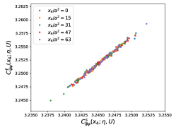
(a) Euclidean time invariance

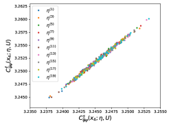
(b) Noise source independence

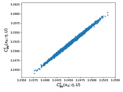
(c) Correlation for training set

Figure 1: Graphical representation of the correlation between the light and strange quark scalar condensates at $t=0$ for several gauge configurations, Euclidean time coordinates and stochastic sources. Left: correlation between light and strange quark scalar condensates for selected values of $x_{4}$. The data shown correspond to the training set of $N_{G,T}=50$ gauge configurations and $N_{\eta}=1$ stochastic source. Middle: Same as the left plot. The data shown correspond to $N_{G,T}=50$, a fixed value of $x_{4}=T/2$ and a selection of stochastic sources. Right: Same as left and middle plots for a single stochastic source, $N_{G,T}=50$ configurations and $T/a=64$ Euclidean time coordinates. This is the set that has been used to train the ML mapping (see Sec. 4).

On these ensembles we have calculated, using stochastic sources as described in the previous section, the Euclidean time dependence of the flowed and unflowed light and strange scalar condensates. On a fixed background gauge configurations, they are defined respectively in Eqs. (10) and (12). We have then analyzed the correlation between the $2$ observables. In Figs. 1(a)- 1(c) we show correlation plots between the light and strange quark condensates at vanishing flow time, $t=0$, calculated on the same ensemble, $M_{1}$. We observe a strong correlation of the data independently on the Euclidean time where we calculate the condensate (see Fig. 1(a)). This is a consequence of translational invariance and is consistent with the observation that averaging over all lattice points provides a better statistical precision, making use of the full lattice. In this context we want to take advantage of translational invariance to enlarge the data set used to train the ML mappings. A similar strong correlation is observed varying the stochastic source used for the determination of the quark propagator (see Fig. 1(b)). This observation allows us to use a relatively small number of gauge configurations for the training. In Fig. 1(c) we show the correlation plot used to train the ML model on the ensemble $M_{1}$, where we have used $N_{G,T}=50$ gauge configurations, all the $64$ Euclidean time values of $x_{4}/a$, and $N_{\eta}=1$ stochastic source. Details on the choice of the training set are discussed in Sec. 4.

For ensembles at lighter pion masses we observe a similar, but slightly weaker, correlation. The weaker correlation could be caused by a generic loss of correlation for lighter pion ensembles or by a larger mass difference between the correlated observables. This does not prevent us to successfully test our ML method also for the ensemble $M_{3}$. We have also observed a similar strong correlation between condensates calculated at different flow times on the same ensembles. The correlation between observables evaluated on the same ensembles is not really surprising, but in the context of ML modelling it provides an interesting observation that could be used to speed-up the calculation of observables from lattice QCD simulations.

4 Decision tree mapping of correlations

To take advantage of the correlations observed and described in the previous section we have scrutinized a few supervised machine learning methods and we have found that a decision tree (DT) is sufficient to capture the correlation between data. There are perhaps other maps, like specific neural networks, that might be able to describe the correlations equally well or even better in certain cases, but for this first investigation DT is sufficiently accurate.

4.1 Description of the algorithm

Decision Tree (DT) stands as a non-parametric supervised learning technique employed for regression tasks involving the prediction of continuous numerical outcomes, by recursively partitioning the input space into subsets based on feature conditions and assigning a constant value to each resulting region.  [17, 18]. The primary aim is to build a model that can predict the value of a target variable by acquiring basic decision rules deduced from the features of the data.

The method we proposed, labeled dtcorr, aims at determining fermionic disconnected diagrams at a given quark mass, or flow time, given a fermionic disconnected diagram calculated at a different quark mass or flow time. dtcorr takes a subset of the total amount of data to train a ML model, a DT in this case, and calculate the corresponding bias. To train the DT we divide the total set of data $N$ into labeled, $N_{L}$, and unlabeled data, $N_{U}$. The labeled data are divided into the subset $N_{T}$ to train the machine learning (ML) model, and the subset $N_{B}$ to estimate the bias correction, with $N_{L}=N_{T}+N_{B}$. The data we consider in this numerical experiment are fermionic disconnected diagrams calculated at $2$ different quark masses or flow times. If we denote with $N_{\eta}$ the number of stochastic sources, $N_{G}$ the number of gauge configurations, and we make use of translational invariance, we can use as a complete set of data for a given condensate $N=N_{\eta}\times N_{G}\times T/a$ points. As labeled data we consider the subset constituted by $N_{L}=N_{\eta,L}\times N_{G}\times T/a$, further divided into the training set $N_{T}=N_{\eta,L}\times N_{G,T}\times T/a$ and the bias correction set $N_{B}=N_{\eta,L}\times N_{G,B}\times T/a$, where $N_{G}=N_{G,T}+N_{G,B}$. Once the ML model has been trained it is applied to the unlabeled data $N_{U}=N_{\eta,U}\times N_{G}\times T/a$, where $N_{\eta,U}=(N_{\eta}-N_{\eta,L})$. This implies that, fixed the labeled data, we have a single DT model for each pair of observables and each ensemble.

To exemplify we want to determine an observable $O$ for given values of external parameters like the quark mass $m$ or the flow time $t$. The DT is trained using as features the same observable at different values of the quark mass or flow time, $O_{f}$, on a subset, the training set, of the total amount of data. The mapping obtained with this training between the $2$ observables is denoted as $\Gamma_{f}$, where the subscript $f$ reminds us that the mapping depends on the choice of the external parameters. In Sec. 4.3 we show that the mapping is independent on the choice and size of the training set.

After the training, the target quantity $O_{\Gamma}(U,\eta,x_{4})$ is obtained by applying the ML mapping to the features on the unlabeled data, i.e.

$$O_{\Gamma}(U,\eta,x_{4})=\Gamma_{f}[O_{f}(U,\eta,x_{4})]\,.$$ (19)

The dependence of $O_{\Gamma}$ on the external parameters $m$, and $t$ is left implicit. We keep explicit the dependence on the variables $U,\eta,x_{4}$ labelling the data set. The ML mapping $\Gamma_{f}$ does not depend explicitly on the training data, but it is evaluated on features that depend on the specific gauge configuration, stochastic source, and Euclidean time and thus so is the output observable.

The correlation function is then obtained averaging on the unlabelled data

$$\frac{1}{N_{G}}\sum_{U}\frac{1}{N_{\eta,U}}\sum_{\eta_{U}}O_{\Gamma}(U,\eta_{U},x_{4})\,,$$ (20)

where with $\sum_{U}$ we indicate a sum of the gauge configurations and $\sum_{\eta_{U}}$ indicates the sum over all the sources belonging to the unlabelled data. In Sec. 4.2 we discuss the results including a bias correction.

The first example we consider is $O_{f}=C^{s}_{\overline{\psi}\psi}(x_{4};\eta,U)$, i.e. the strange scalar quark condensate, and $O=C^{l}_{\overline{\psi}\psi}(x_{4};\eta,U)$, i.e. the light scalar quark condensate. Both are defined in Eq. (10). The second example we consider is $O_{f}=C^{l}_{\overline{\chi}\chi}(x_{4},\bar{t};\eta,U)$ i.e. the light quark scalar condensate at flow time $\bar{t}$ , and $O=C^{l}_{\overline{\chi}\chi}(x_{4},t;\eta,U)$, i.e. the same condensate at a different flow time $t$. This quantity is defined in Eq. (16).

The DT mapping, $\Gamma$, is determined on the training set minimizing a loss function given by the mean squared error, and for each node, the algorithm considers all the input data and chooses the best split. Nodes are expanded until all leaves contain a single sample. All other hyper-parameters are kept to their default values.

The mapping is then applied to the unlabeled data of the input quantity for each $N_{\eta,U}=N_{\eta}-N_{\eta,L}$ stochastic source, each gauge configuration, and each $x_{4}/a$. We have performed a study of the integrated autocorrelation time, following the Sokal method [20], and we found that $\tau_{\text{int}}\simeq 2-3$ in all cases scrutinized. To avoid autocorrelation in the training procedure, we have chosen the set of $N_{G,T}=50$ with each gauge maximally separated in the Markov chain. This means that we select gauge configurations separated by $8-9$ gauges. When applying the ML mapping to the unlabeled data, after averaging over the stochastic sources, we build blocks of $10$ elements and then a standard bootstrap procedure is applied with $N_{b}=1000$ bootstrap samples. This permits the calculation of the statistical error of the resulting condensate.

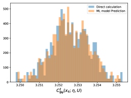
(a) Ensemble $M_{1}$

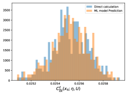
(b) Ensemble $M_{1}$

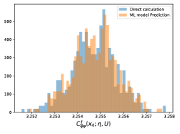
(c) Ensemble $M_{3}$

Figure 2: Distribution on the unlabeled data of quark condensates at $x_{4}=T/2$ from a direct calculation and from the ML mapping.

In total, we have $N_{\eta}=20$ stochastic sources, $N_{G}$ gauges given in Table 1, and for both lattices $T/a=64$ time extent. For the training we use $N_{\eta,L}=1$ stochastic source and $N_{G,T}=50$ gauge configurations. This gives us, for both ensembles, a total of $N_{T}=3200$ data points to train the ML model. In Fig. 2 we show the distributions of $3$ condensates, comparing the distribution obtained from the direct calculation of the condensates and from the ML mapping.

4.2 Results

The results obtained with the ML mapping, cfr. Eq. (20), have been corrected for possible biases. To estimate the bias correction we use the same stochastic source chosen for the training set and the remaining $N_{G,B}=N_{G}-N_{G,T}$ gauges. The bias-corrected result is given by

$$\left\langle O_{\Gamma}\right\rangle_{G,\eta}(m,t,x_{4})=\frac{1}{N_{G}}\sum_{U}\frac{1}{N_{\eta,U}}\sum_{\eta_{U}}O_{\Gamma}(U,\eta_{U},x_{4})+\frac{1}{N_{G,B}}\sum_{U_{B}}\left[O(U_{B},\eta_{L},x_{4})-O_{\Gamma}(U_{B},\eta_{L},x_{4})\right]$$ (21)

where the bias correction is evaluated on the bias set. If the bias set contains more than one stochastic source the second term in Eq. (21) is averaged over the number of sources in the bias set.

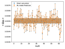
(a) Without bias correction

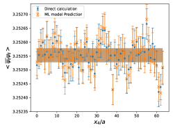
(b) With bias correction

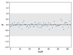
(c) Deviation between the direct and the ML calculation normalized with the total standard deviation (see main text)

Figure 3: Comparison of the light quark condensate on the ensemble $M_{1}$ between the ML result and the direct (standard) calculation of the same condensate as a function of Euclidean time. The comparison is performed on the unlabelled data.

We have determined the light quark condensate at $t=0$ training the ML mapping as described in the previous section using the strange quark condensate as features. We have then calculated the bias corrections as described above. We have also use a ML mapping to determine the flowed scalar quark condensate on a set of flow times. The features used to train the ML mapping are the light quark condensate at $t/a^{2}=0.5$ for the ensemble $M_{1}$ and $t/a^{2}=1$ for the ensemble $M_{3}$.

Results after the training are shown in Figs. (3 - 5), where the ML results (orange data) are compared with a standard determination of the same condensates on the unlabelled of data (blue data). With this choice both the standard and the ML determinations use a common set of data simplifying the comparison of statistical errors. Figs. 3 and 5 show the results for the light quark condensate at $t/a^{2}=0$ for the $2$ ensembles $M_{1}$ and $M_{3}$. The ML mappings are obtained using the strange quark condensate on the same ensembles. Fig. 4 shows the result for the light quark condensate at $t/a^{2}=0.7$ obtained with a ML mapping trained with features given by the same condensate at $t/a^{2}=0.5$.

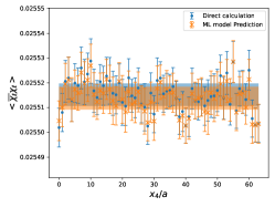
(a) Without bias correction

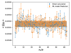
(b) With bias correction

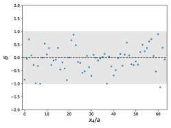
(c) Deviation between the direct and the ML calculation normalized with the total standard deviation (see main text)

Figure 4: Comparison of the light quark condensate on the ensemble $M_{1}$ at flow time $t/a^{2}=0.7$ between the ML result and the direct (standard) calculation of the same condensate as a function of Euclidean time. The comparison is performed on the unlabelled data.

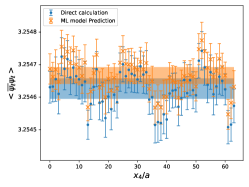
(a) Without bias correction

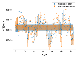
(b) With bias correction

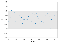
(c) Deviation between the direct and the ML calculation normalized with the total standard deviation (see main text)

Figure 5: Comparison of the light quark condensate on the ensemble $M_{3}$ between the ML result and the direct (standard) calculation of the same condensate as a function of Euclidean time. The comparison is performed on the unlabelled data.

For these $3$ cases, in the left plots we show the comparison between the ML and the direct determinations before any bias correction is applied, while the middle plots are obtained after bias correction. The right plots show the deviation between the direct and the ML calculation normalized with the total standard deviation

$$\delta=\frac{\left\langle O\right\rangle(x_{4})-\left\langle O_{\Gamma}\right\rangle(x_{4})}{\sqrt{\sigma^{2}_{O_{\Gamma}}+\sigma^{2}_{O}}}\,.$$ (22)

The statistical errors are calculated as follows. First, we apply the ML mapping to the unlabeled data, after averaging over the stochastic sources, then we build blocks of $10$ elements and a standard bootstrap procedure is performed with $N_{\text{boot}}=1000$ bootstrap samples. In this way, we determine the error bars of both the condensate for each $x_{4}/a$, and the average over Euclidean time.

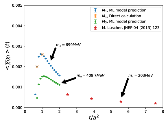
Figure 6: Flow time dependence of the light quark scalar condensate. The plot shows the results obtained with a ML mapping and the results obtained in Ref. [8]. With orange crosses we also indicate flow times where we have available a direct calculation.

Using ${\tt dtcorr}$ we have determined the light quark condensate as a function of flow time in the region $0\leq t/a^{2}\leq 2$ for the $2$ ensembles $M_{1}$ and $M_{3}$. The features used to train the ML mapping are the light quark condensate at $t/a^{2}=0.5$ for the ensemble $M_{1}$ and $t/a^{2}=1$ for the ensemble $M_{3}$. We present the ML results in Fig. 6 where we show the light quark condensate as a function of flow time $t/a^{2}$. In the same plot we also show for comparison the direct calculation at $t/a^{2}=0.7,~{}1$ for the ensemble $M_{1}$ and the results obtained in Ref. [8] with a direct calculation of the disconnected diagrams. The small flow time region covered by the ML calculation shows the power divergent contribution proportional to $m/t$ and possibly other power divergent contributions vanishing in the continuum limit. In the chiral and continuum limit Ward identities connect the flowed condensate with the physical condensate [8, 21], and the power divergence in $1/t$ vanishes. In Fig. 6 we observe, at short flow time, the $1/t$ contribution that is suppressed at lower quark masses. For larger flow times and smaller quark masses, as described in Ref. [8], the $1/t$ contribution is small and the remaining logarithmic contribution is cancelled by the contribution of the vacuum-to-pion pseudoscalar matrix element evaluated at the same flow time.

4.3 Robustness of the ML mapping

To test the robustness of ${\tt dtcorr}$ we have varied specific hyperparameters, like the number and the choice of gauge configurations and stochastic sources used for the training. We have studied the dependence on the choice of the training set considering different, randomly chosen, sets of $N_{G,T}=50$ gauge configurations and different choices for the stochastic source.

In Fig. 7 we show the ML calculation for $10$ different random choices of the $N_{G,T}=50$ gauge configurations used for the training, and compare it with the full direct calculation of the complete set of data. We hardly observe any deviation between all the calculations. In Fig. 8 we show the dependence of the ML calculations on the choice of the stochastic source and on the number of gauge configurations, $N_{G,T}$, used for the training. We observe no significant deviation when we choose a different stochastic source or when we vary the size of the training set. We conclude that changing the training set or its size results in little to no deviation between the different ML mappings obtained and the direct standard calculation.

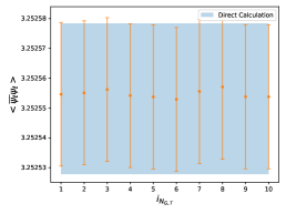
(a) $\left\langle\overline{\psi}_{\ell}\psi_{\ell}\right\rangle$ from ensemble $M_{1}$

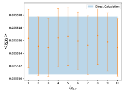
(b) $\left\langle\overline{\chi}_{\ell}\chi_{\ell}\right\rangle$ at $t/a^{2}=1$ from ensemble $M_{1}$

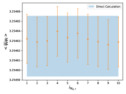
(c) $\left\langle\overline{\psi}_{\ell}\psi_{\ell}\right\rangle$ from ensemble $M_{3}$

Figure 7: Results for the light quark condensates for $10$ different training sets, labeled by $i_{N_{G,T}}$, obtained selecting randomly $N_{G,T}=50$ gauge configurations among the full ensemble. The blue band represents the calculation of the light quark condensate on the full set of data $N_{\eta,U}$

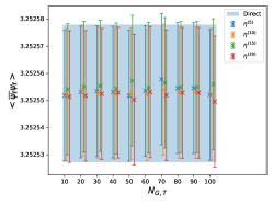
(a) $\left\langle\overline{\psi}_{\ell}\psi_{\ell}\right\rangle$ from ensemble $M_{1}$

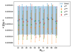
(b) $\left\langle\overline{\chi}_{\ell}\chi_{\ell}\right\rangle$ at $t/a^{2}=1$ from ensemble $M_{1}$

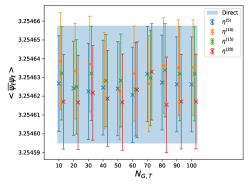
(c) $\left\langle\overline{\psi}_{\ell}\psi_{\ell}\right\rangle$ from ensemble $M_{3}$

Figure 8: Dependence of the quark condensates on the choice of stochastic sources and the size of the training set. The direct calculation, referring to the standard calculation using the full set of data $N_{\eta,U}$, is compared with the ML mapping prediction using in the training set different single stochastic sources, $\eta^{(r)}$, $r=5,~{}10,~{}15,~{}20$, and different numbers of gauge configurations, $N_{G,T}$. The bias correction is calculated with $N_{G,B}=N_{G}-N_{G,T}$ gauge configurations and the same stochastic source

5 Conclusions

We have investigated an application of supervised Machine Learning (ML) techniques for lattice QCD calculations. Fermionic disconnected diagrams are among the most expensive quantities to calculate in any lattice QCD computation. We have proposed a simple method, ${\tt dtcorr}$, to speedup the calculation of fermionic disconnected diagrams for a set of external parameters such as the quark mass and the flow time. The ML mapping is a decision tree trained with a subset of the full set of data usually analyzed for a standard lattice QCD calculation. After applying a small bias correction, we find that the condensates calculated with ML deviate at most by $1$ sigma over the whole set of parameters investigated.

The computational gain depends whether the ML mapping is trained using $2$ different quark masses or $2$ different flow times. In the first case the time needed using ${\tt dtcorr}$ is

$$t_{\text{ML}}=\left(\frac{t_{s}}{t_{d}}\frac{N}{N_{U}}+\frac{N_{L}}{N_{U}}\right)\times t\,,$$ (23)

where $t_{d,s}$ label the time needed to calculate the down, or strange, condensate for a single stochastic source and single gauge configuration, while $t$ is the total time needed for a standard lattice QCD calculation. We have estimated the timings for the calculation of the quark propagators, and conclude that the ML calculation requires $68-78\%$ of the time needed for a standard computation. The gain depends almost solely on the difference in computer time needed for the calculation of the $2$ quark propagators used in the ML method. The gain will certainly become larger for lighter pion ensembles, where the difference between the strange and quark mass is larger. It remains to be seen if enough data correlation survives in order to apply our ML method.

In this case of different flow times the gain obviously depends on the number of flow times $N_{t}$ where the condensate is determined, with gains varying from about a factor $2$ to about a factor $20$, which is the maximal gain given the size of the labelled and unlabelled data.

Machine Learning methods can provide powerful computational tools to make better use of the plethora of data produced in standard lattice QCD calculations. In this work we have successfully applied a supervised ML method to speed-up the calculation of disconnected fermionic diagrams. We consider this work as a first attempt into the exploration of novel paths for the determination of the quark propagator and fermionic correlation functions in lattice QCD simulations.

References

- [1] A. Alexandru, P. F. Bedaque, H. Lamm, S. Lawrence, Deep Learning Beyond Lefschetz Thimbles, Phys. Rev. D 96 (9) (2017) 094505. arXiv:1709.01971, doi:10.1103/PhysRevD.96.094505.
- [2] W. Detmold, G. Kanwar, H. Lamm, M. L. Wagman, N. C. Warrington, Path integral contour deformations for observables in gauge theory, Phys. Rev. D 103 (9) (2021) 094517. arXiv:2101.12668, doi:10.1103/PhysRevD.103.094517.
- [3] J.-L. Wynen, E. Berkowitz, S. Krieg, T. Luu, J. Ostmeyer, Machine learning to alleviate Hubbard-model sign problems, Phys. Rev. B 103 (12) (2021) 125153. arXiv:2006.11221, doi:10.1103/PhysRevB.103.125153.
- [4] A. Witt, J. Kim, C. Körber, T. Luu, ILP-based Resource Optimization Realized by Quantum Annealing for Optical Wide-area Communication Networks – A Framework for Solving Combinatorial Problems of a Real-world Application by Quantum Annealing (1 2024). arXiv:2401.00826.
- [5] J. Kim, W. Unger, Error reduction using machine learning on Ising worm simulation, PoS LATTICE2022 (2023) 018. arXiv:2212.02365, doi:10.22323/1.430.0018.
- [6] B. Yoon, T. Bhattacharya, R. Gupta, Machine Learning Estimators for Lattice QCD Observables, Phys. Rev. D 100 (1) (2019) 014504. arXiv:1807.05971, doi:10.1103/PhysRevD.100.014504.
- [7] M. Lüscher, Properties and uses of the Wilson flow in lattice QCD, JHEP 08 (2010) 071, [Erratum: JHEP 03, 092 (2014)]. arXiv:1006.4518, doi:10.1007/JHEP08(2010)071.
- [8] M. Lüscher, Chiral symmetry and the Yang–Mills gradient flow, JHEP 04 (2013) 123. arXiv:1302.5246, doi:10.1007/JHEP04(2013)123.
- [9] A. Shindler, J. de Vries, T. Luu, Beyond-the-Standard-Model matrix elements with the gradient flow, PoS LATTICE2014 (2014) 251. arXiv:1409.2735, doi:10.22323/1.214.0251.
- [10] A. Shindler, Moments of parton distribution functions of any order from lattice QCD (11 2023). arXiv:2311.18704.
- [11] J. Foley, K. Jimmy Juge, A. O’Cais, M. Peardon, S. M. Ryan, J.-I. Skullerud, Practical all-to-all propagators for lattice QCD, Comput. Phys. Commun. 172 (2005) 145–162. arXiv:hep-lat/0505023, doi:10.1016/j.cpc.2005.06.008.
- [12] M. Foster, C. Michael, Quark mass dependence of hadron masses from lattice QCD, Phys. Rev. D 59 (1999) 074503. arXiv:hep-lat/9810021, doi:10.1103/PhysRevD.59.074503.
- [13] P. Boucaud, et al., Dynamical Twisted Mass Fermions with Light Quarks: Simulation and Analysis Details, Comput. Phys. Commun. 179 (2008) 695–715. arXiv:0803.0224, doi:10.1016/j.cpc.2008.06.013.
- [14] S. Heather M., A. Stathopoulos, E. Romero, J. Laeuchli, K. Orginos, Probing for the Trace Estimation of a Permuted Matrix Inverse Corresponding to a Lattice Displacement, SIAM J. Sci. Comput. 44 (4) (2022) B1096–B1121. arXiv:2106.01275, doi:10.1137/21M1422495.
- [15] S. Aoki, et al., Non-perturbative renormalization of quark mass in QCD with the Schroedinger functional scheme, JHEP 08 (2010) 101. arXiv:1006.1164, doi:10.1007/JHEP08(2010)101.
- [16] S. Aoki, et al., 2+1 Flavor Lattice QCD toward the Physical Point, Phys. Rev. D 79 (2009) 034503. arXiv:0807.1661, doi:10.1103/PhysRevD.79.034503.
-
[17]
L. Breiman, J. Friedman, C. Stone, R. Olshen,
Classification and
Regression Trees, Taylor & Francis, 1984.
URL https://books.google.de/books?id=JwQx-WOmSyQC - [18] L. Breiman, Classification and regression trees, Routledge, 2017.
- [19] F. Pedregosa, et al., Scikit-learn: Machine Learning in Python, J. Machine Learning Res. 12 (2011) 2825–2830. arXiv:1201.0490.
- [20] U. Wolff, Monte Carlo errors with less errors, Comput. Phys. Commun. 156 (2004) 143–153, [Erratum: Comput.Phys.Commun. 176, 383 (2007)]. arXiv:hep-lat/0306017, doi:10.1016/S0010-4655(03)00467-3.
- [21] A. Shindler, Chiral Ward identities, automatic O(a) improvement and the gradient flow, Nucl. Phys. B 881 (2014) 71–90. arXiv:1312.4908, doi:10.1016/j.nuclphysb.2014.01.022.
- [22] JURECA: Data Centric and Booster Modules implementing the Modular Supercomputing Architecture at Jülich Supercomputing Centre, Jounal of large-scale research facilities (JLSRF) 7 (2021) A182. doi:10.17815/jlsrf-7-182.