Logical Synchrony Networks: A formal model for deterministic distribution

Abstract

KPN are a deterministic MoC for distributed systems. KPN supports non-blocking writes and blocking reads, with the consequent assumption of unbounded buffers between processes. Variants such as FFP have been developed, which enforce boundedness. One issue with existing models is that they mix process synchronisation with process execution. In this paper we address how these two facets may be decoupled.

This paper explores a recent alternative called bittide, which decouples the execution of a process from the control needed for process synchronisation, and thus preserves determinism and boundedness while ensuring pipelined execution for better throughput. Our intuition is that such an approach could leverage not only determinism and buffer boundedness but may potentially offer better overall throughput.

To understand the behavior of these systems we define a formal model – a deterministic MoC called LSN. LSNs describes a network of processes modelled as a graph, with edges representing invariant logical delays between a producer process and the corresponding consumer process. We show that this abstraction is satisfied by KPN. Subsequently, we show that both FFP and bittide faithfully implement this abstraction. Thus, we show for the first time that FFP and bittide offer two alternative ways of implementing deterministic distributed systems with the latter being more performant.

=-15pt

FIFO

I Introduction

Table I: Communication Schemes for Synchronisation

Scheme	Writers	Readers	Buffer Size	Blocking Read	Blocking Write	Triggering	Decoupling
Unsynchronized	Many	Many	One	No	No	None	No
Read-Modify-Write	Many	Many	One	Yes	Yes	Event	No
Unbounded *FIFO	Single	Single	Unbounded	Yes	No	Event	No
Bounded *FIFO	Single	Single	Bounded	Yes	Yes	Event/Schedule	No
Rendezvous	Single	Single	One	Yes	Varies	Event	No
Time Triggered	Single	Varies	One/Bus-based	No	No	Physical Clock	No
Elastic Buffer [1]	Single	Single	Bounded	No	No	Logical Clock	Yes

MoC [2] are used to formally describe how concurrent components of a system are composed, focussing on their computation and the communication. For the design of distributed systems, many MoC have been developed, which range from non-deterministic models such as process algebras [3, 4] and actor-based models [5] to deterministic variants based on KPN [6] and synchronous models [7]. MoC require a communication scheme for physically distributed components. Edwards et al. [8] categorize communication common schemes as follows (see Table I):

• Unsynchronized: No coordination between transmissions and receives. There is no guarantee on the safe arrival of data.

• Read-Modify-Write: Processes communicate over shared memory. Each process locks a shared variable for the duration of its access, then unlocks it.

• Unbounded FIFO: A sender process generates data tokens which are consumed by a receiver in-order. The intermediate medium can hold any number of tokens which are awaiting consumption. A receiver cannot progress without consuming a token.

• Bounded FIFO: A sender process generates data tokens which are consumed by a receiver in-order. The intermediate medium can hold at most a finite number of tokens away consumption. A sender cannot progress without free buffer capacity, nor can a receiver progress without consuming a token.

• Rendezvous: Processes synchronise according to explicit messaging between processes. A process reaching a ‘send’ or ‘receive’ action must stall until the corresponding event is reached at another.

In addition, we include the following mechanisms not present in [8].

• Time triggered: Processes synchronise using known timing bounds, and coordinate clocks using clock synchronisation protocols [9].

• Elastic Buffer: A very recent mechanism proposed in bittide [10]. These provide FIFO boundedness without the need for blocking reads or writes. Instead, the buffer management is implicitly handled through a control mechanism where each node adjusts its frequency based on the rate of communication with its neighbours.

The characteristics of each are summarised in Table I, compared by the number of writers and readers (i.e. point-to-point or broadcast communication), the size of intermediate buffers, and whether blocking I/O is required for correct execution. Triggering refers to the mechanism which drives each communication event. Most schemes are event-triggered, meaning communication occurs as a result of reaching specific points in execution. This may be paired with a static schedule of execution events. On the other hand, clocked schemes use synchronisation that is driven periodically by a clock. Clocks may be either physical, where synchronisation uses physical time or logical, where logical time, like in synchronous programmes [7], is used for synchronisation. Decoupled schemes are those where synchronisation behaviour does not interfere with execution behaviour of a process, meaning each process remains free-running without blocking or awaiting an event or elapsed time.

I-A Deterministic models

We focus on deterministic models since they are ideally suited for the design of safety critical systems. FIFO-based models, where every pair of producer and consumer are connected using point to point buffers, is of considerable interest for deterministic systems. Kahn’s seminal work formalises KPN models [6], where a producer never blocks, while a consumer blocks while accessing an empty FIFO. When a consumer blocks on a given FIFO, it is prevented from context switching and hence this model is shown to be determinate [6], i.e. for any arbitrary execution order of the processes, the order of tokens in the buffers remains invariant. However, the scheduling problem using bounded memory is undecidable. Hence, variants such as FFP [11] introduce blocking on both the producer side (when the FIFO is full) and consumer side (when the FIFO is empty). As the shared buffer usually resides with one of the two processes, the other process needs an estimation of the buffer size. In [11] an approach called back pressure LTTA is introduced to determine the buffer capacity. We observe that for synchronization, existing deterministic models either use physical time or intertwine process execution with synchronisation, leading to undesirable inefficiencies. In this paper, we move away from both these approaches using a recent protocol called bittide [10].

I-B The bittide Approach

While FFP guarantee determinism, the overall performance of the system is dependent on the number of times during execution when processes block, i.e. as each process executes its tick, it may need to execute a skip cycle, where no data is sent / received from the FIFO. Hence, the overall available parallelism is restricted by these skip cycles. How can this be mitigated?

Recently, Google has developed a physical layer protocol called bittide [10]. Like FFP bittide also uses point to point FIFO buffers (called elastic buffers) for communication. However, in bittide, the issue of computation of a process (its execution model) is decoupled from its synchronisation model with other processes.. Each process executes using its local clock. When the clock ticks, the sender process writes to its elastic buffer. Likewise, when the consumer clock ticks, a token is removed from its FIFO buffer.

It is obvious that mismatching frequencies of the producer and consumer will cause buffer overflow / underflow. However, in bittide, this is handled by distributed controllers at each process. The controllers examine the local buffer at a process to determine the relative speed of the neighbours. Using this as a feedback signal, appropriate controllers are designed, which ensure that frequencies of all processes stabilise to a common frequency, ensuring buffer boundedness. This protocol has been shown to be both deterministic and performant. However, several key aspects of this protocol need further investigation.

II Related Work

Process synchronisation may be physical time-based, such as in the family of TTA [12], which employ hardware clock synchronisation. Similarly, the recent language Lingua Franca [13] employs a physical synchronisation protocol based on Ptides [14]. Using known latency bounds, each process can locally decide a “safe-to-process” time to proceed. When these bounds are violated, the system flags a fault and invokes a handler. While robust, Lingua Franca primarily focuses on the mixture of logical and physical time to ensure the safe execution of safety-critical system, rather than the logical synchrony approach of abstracting away physical time in distributed systems.

LTTA [15] describe a family of protocols, which preserve synchronous semantics over quasi-periodic architectures. While the specific protocol varies, all designs synchronise logical tick progression through the use of explicit messaging. As a result, throughput is inversely proportional to the length of transmission delays. In general, the communication delays are assumed to be small relative to the task duration.

GALS models are those which preserve synchronous semantics within a single machine, but communicate over asynchronous mediums. Here, the shared notion of time may be eliminated altogether. Such designs may introduce non-determinism at a system level. When distributing over GALS architectures, certain designs can remain deterministic by construction or through the synthesis of wrappers. Generally, this is achieved by stalling a process when an unresolved dependency is reached, forcing a design to be event-triggered rather than clock-triggered. Thus, the system experiences desynchronisation and corresponding resynchronisation [16, 17]. Processes capable of behaviourally correct resynchronisations are called endochronous [18], but determining endochrony in general is a difficult task.

II-A Contributions

We make the following contributions for the design of deterministic and performant distributed systems:

1. We formalise LSN, recently introduced in [1], in the context of deterministic MoC for distributed systems.

2. We show KPN are LSN instance.

3. We show that bittide [10], is also a realisable LSN instance. We introduce a variant of FFP called LSFP for making a fair comparison with bittide (see Section VI-B for details).

4. We present an empirical evaluation of the performance of LSFP and bittide, and we show that bittide is more performant in the average case.

This paper is organized as follows: in Section III, we introduce our definition of LSN, adapted from [1]. Two realisable implementations are demonstrated. In Section IV we show that the well-known KPN model can be used to express LSN. Similarly, the recent physical-layer protocol bittide is shown to express LSN in Section V. In Section VI we show how FFP implement KPN, and thus propose LSFP as a restriction which implements the LSN model efficiently. Then, Section VII compares the performance of FFP relative to bittide. Finally, Section VIII makes concluding remarks including future directions.

III Logically Synchronous Networks

We provide a generic, graph-based abstraction of a distributed system comprising a network of machines $\mathscr{M}_{i}$, denoting the $i-th$ machine, which labels the vertex $v_{i}$, as introduced recently in [1]. Furthermore, we formalise the LSN model, in this paper, to show that existing models of computations, especially those based on KPN, exhibit the LSN property of invariant logical delays, elaborated next.

Machines execute at discrete points called events or ticks. Each machine has its own notion of ticking, which may be different from other machines. The event count $\theta_{i}\in\mathbb{N}$, corresponding to the machine $\mathscr{M}_{i}$ increases by 1 every tick. The defining feature of LSN is the invariant logical delays, meaning there always exists an invariant offset between the event count of any production events and their associated consumption events along a channel.

An event is denoted ($\mathscr{M}_{i}$, $\theta_{i}$), where $\mathscr{M}_{i}$ is the machine experiencing the event when $\theta_{i}$ is its event counter. We say that two events $(\mathscr{M}_{i},\theta_{i})\prec(\mathscr{M}_{j},\theta_{j})$ iff $\theta_{j}-\theta_{i}=\lambda_{i\rightarrow j}$. At each event, a token is read from each input edge and a token is produced to each output edge. The event count $\theta_{i}\in\mathbb{N}$ increases by 1.

Definition 1.

LSN is a tuple $<G,\Theta,\lambda>$, where:

• $G{=}{<}V,E{>}$ is a digraph where $V$ denotes a set of vertices, and $E$ $\subseteq V{\times}V$ denotes a set of edges such that $v1\neq v2$ for all $(v1,v2)\in E$.

• Each vertex $\mathscr{M}_{i}\in V$ corresponds to a machine executing a synchronous program that generates an event every tick. $\theta_{i}\in\Theta$ represents the event counter for the machine $\mathscr{M}_{i}$ and the value of $\theta_{i}\in\mathbb{N}$. As the next event is generated by a machine as its ticks, its event counter is incremented by 1.

• Edges are labelled with the logical delay mapping $\lambda:E\rightarrow\mathbb{Z}$. Moreover, $\lambda((\mathscr{M}_{i},\mathscr{M}_{j}))=\lambda_{i\rightarrow j}$ implies the following relation holds between the events associated with this edge: $(\mathscr{M}_{i},\theta_{i})\prec(\mathscr{M}_{j},\theta_{j})$. Consequently, $\theta_{j}-\theta_{i}=\lambda_{i\rightarrow j}$.

Example III.1.

An example LSN is shown in LABEL:fig:lsn_example, consisting of three machines $M_{i},M_{j},M_{k}$. An example edge is between $(M_{k},M_{j})$, which is labelled with a value 2, which indicates the invariant logical delay, denoted $\lambda_{k\rightarrow j}$, between production of some event at $M_{k}$ and consumption at $M_{j}$ at any tick of the two machines when the production and the corresponding consumption happens. For this edge $\lambda_{k\rightarrow j}=2$.

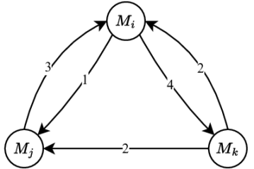
Figure 1: A three-node *LSN

figure]fig:lsn_example

Definition 2.

LSN execution forms CPO of events, known as the extended graph $G_{ext}={<}V_{ext},E_{ext}{>}$.

• $V_{ext}$ is the set of all machine events in the network, described by $V_{ext}=\{(\mathscr{M}_{i},n)|\mathscr{M}_{i}\in V,n\in\theta_{i}\}$

• $E_{ext}$ describes the directed edges showing dependencies between events, which are of the following two types.

  1. Edges between events at different machines $(\mathscr{M}_{i},n){\rightarrow}(\mathscr{M}_{j},m)$ are called communication edges, corresponding to an edge $(\mathscr{M}_{i},\mathscr{M}_{j})\in E$ in the LSN. The clock difference $m{-}n$ is the associated logical delay $\lambda_{i\rightarrow j}$

  2. Edges between successive events at the same machine $(\mathscr{M}_{i},n){\rightarrow}(\mathscr{M}_{i},n+1)$ are called computation edges, which capture monotonicity of local machine events.

Due to the condition on LSN that all cycles in the graph are positive, the corresponding ordering relation is monotonic and acyclic by construction. We assume a finite execution, meaning there is a unique start-up event $\bot$, which precedes the first event at each machine, and termination event $\top$, which succeeds the final event at each machine. These two events forms the greatest lower bound and least upper bounds of the orderings respectively. $G_{ext}$ for the example shown in LABEL:fig:lsn_example is demonstrated in Figure 2.

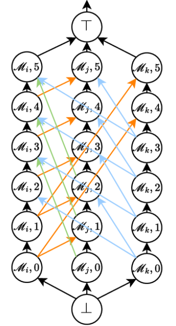
Figure 2: $G_{ext}$ of the three-machine *LSN (LABEL:fig:lsn_example). Computation edges shown in black and communication edges coloured to differentiate source machine

The defining feature of LSN is the invariant logical delays, meaning there always exists an invariant offset between the event count of any production events and their associated consumption events along a channel. The same invariance applies over both edges and paths. Multiple paths, with different cumulative logical delays, may exist between any two machines. $\lambda_{i\rightarrow{j}}$. This does not imply that the machines have any relationship between event counts at any one physical time when observed by a global entity; any amount of physical time may have elapsed between the two events.

Example III.2.

Figure 3 shows an example event sequence for the LSN in LABEL:fig:lsn_example with a potential execution trace of the three machines and their relationship in both logical and physical time. The three machines are desynchronised in their event timings in physical time. However, the logical time offset remains invariant.

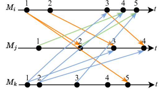
Figure 3: The execution trace of the three-machine *LSN (LABEL:fig:lsn_example), as measured by a global observer

III-A Relabelling of Logical Delays

An interesting facet of the LSN model is the possibility of negative logical delays. Consider that if each machine in a network gets powered on at a different physical time, then there is no meaningful relationship between the initial clock values. As a result, the invariant logical delay along some edges can be non-positive. However, any path in the network forming a cycle must have a positive and invariant summation of logical delays (as a machine cannot send to its own previous events).

The logical delay along specific paths may be manipulated freely, as long as the total summation in each cycle is preserved. In [1] it is proven that all LSN with negative delays have at least one all-positive counterpart. We describe one startup protocol through which relabelling can be achieved:

Example III.3.

Consider a network with some negative logical delays shown in LABEL:fig:negativedelay. An execution trace slice is shown in LABEL:fig:negativetrace. Note how signals from $\mathscr{M}_{j}$ to $\mathscr{M}_{k}$ transmit forwards in physical time, but backwards in logical time due to the clock offsets.

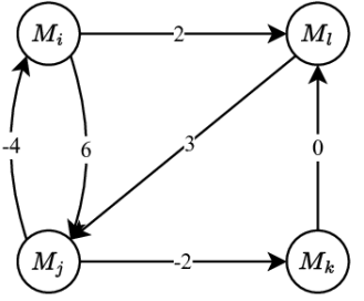
Figure 4: A four-machine *LSN with negative edges

figure]fig:negativedelay

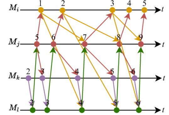
Figure 5: The execution trace of the four-machine *LSN with negative edges (LABEL:fig:negativedelay)

figure]fig:negativetrace

Take a root machine in the graph to act as the initiator. From there, choose a spanning tree to all other machines. Prior to any execution, the initiator node can propagate the startup signal along this tree. Each clock resets its clock counter to zero and begins executing, resulting in a logical delay of zero along each tree edge.

To satisfy the invariance condition in every graph cycle, the LSN edges which are not part of the tree will naturally take on the residual logical delay. By using more sophisticated startup signals (e.g. start after $n$ ticks) various relabellings can be achieved. This protocol for our running example is demonstrated in LABEL:fig:relabelling. The initiator node and edges belonging to the spanning tree are highlighted in green. Note that the summation of each graph cycle from LABEL:fig:negativedelay is preserved. The corresponding execution trace is shown in LABEL:fig:relabelledtrace.

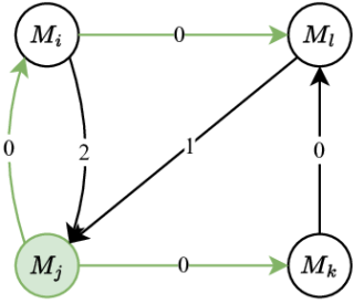
Figure 6: The four-machine *LSN from LABEL:fig:negativedelay after an equivalent relabelling)

figure]fig:relabelling

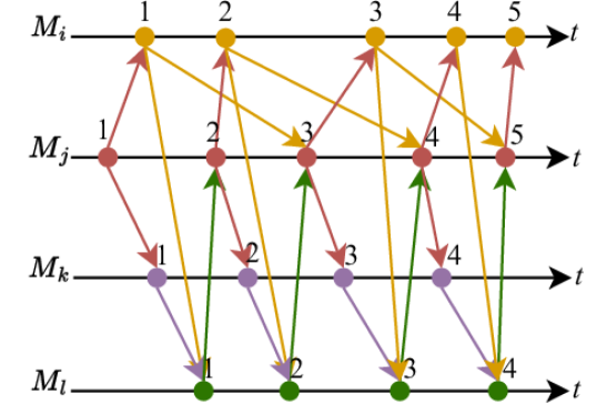
Figure 7: The four-machine execution trace from LABEL:fig:negativetrace after an equivalent relabelling

figure]fig:relabelledtrace

III-B Determinism

In order to reason about LSN behaviours, we start by abstracting machines as mathematical functions. Each machine $\mathscr{M}_{i}\in V$ has a corresponding function $f_{i}\in\mathscr{F}$, where $\mathscr{F}$ is the set of all machine functions, which can be described as a synchronous Mealy machine:

$$f_{i}:X^{N}\times S_{i}\rightarrow X^{M}\times S_{i}$$ (1)

Where $X^{N}$ denotes a vector of inputs and $X^{M}$ denotes a vector of output values from that machine. $S_{i}$ denotes the set of states for $\mathscr{M}_{i}$. The function takes in all current inputs and the current state, and produces some outputs and the next state.

Consider again our extended graph $G_{ext}$. Each event is associated with a corresponding function instantiation, where $f_{i}^{0}$ represents the first invocation of machine $\mathscr{M}_{i}$ at event $(\mathscr{M}_{i},0)$, and $f_{i}^{k-1}$ the $kth$ invocation at $(\mathscr{M}_{i},k-1)$. The input and output edges of an event form the input and output vectors respectively and the state corresponds to the event.

Determinism has a variety of different interpretations in literature as summarised in [19]. In this context we interpret it as follows:

Definition 3.

LSN system is determinate if for any two or more executions with consistent initial conditions, the resulting output traces are consistent, where:

• The output derived from the initial condition consists of the function instance applied to the initial event, $\bot$.

• An output trace for a single machine consists of the sequence of outputs from each function instance $\langle\mathbf{f^{i}}\rangle=\langle f_{i}^{0}::f_{i}^{1}::...::f_{i}^{n-1}\rangle$ where $::$ is the concatenation operator.

Lemma 1.

Consider any event $(M_{i},n)\in V_{ext}$. The value of any edge (incoming/outgoing) is determinate.

Proof:

Any edge is a composition of functions and hence determinate. ∎

Theorem 1.

LSN execution is always determinate.

Proof:

Based on Lemma 1 and by induction on the depth $k$ of the extended graph corresponding to the LSN. Note that any event is only dependent on events that happened prior to it. ∎

IV KPN as an instance of LSN

KPN are a well-known model of computation for deterministic systems. KPN model a network of machines communicating over unbounded FIFO channels. Each machine in KPN executes over discrete firings, analogous to LSN events, where at each firing a token is consumed from every inbound FIFO, and a token pushed onto each outbound FIFO.

Definition 4.

KPN is denoted as a graph $G^{\prime}=<V^{\prime},E^{\prime}>$ and a labelling function $\alpha:E^{\prime}\rightarrow B$ where any $b\in B$ is an unbounded FIFO queue. Each buffer has an associated occupancy of tokens given by $\beta:B\times\mathbb{R}\rightarrow\mathbb{N}$, where $\mathbb{R}$ is the current physical time and $\mathbb{N}$ the count of tokens in the FIFO.

A basic two-vertex KPN is shown in Figure 8, with the initial occupancies $\beta(\alpha(p,q),0)=j$ and $\beta(\alpha(q,p),0)=k$. KPN with cyclic components will immediately deadlock if there are no initial tokens. Every directed cycle in a graph must always have at least one token to be live. We call these values the initial marking.

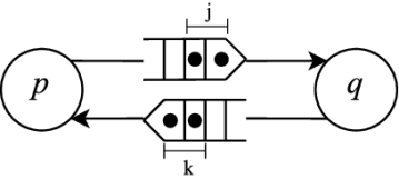
Figure 8: A cyclical *KPN, with some initial tokens in each directional unbounded *FIFO

KPN alone do not describe when a machine may fire, so we introduce a set of firing rules which dictate firing times. Numerous firing orders may be possible with different temporal interleaving of events, as long as FIFO do not underflow. Conventionally this is avoided through use of blocking channel reads.

IV-A LSN to KPN Refinement

By observation of the graphical similarities between LSN and KPN, and the effect of initial FIFO markings on delays, we can deduce a simple transformation.

Observation 1.

Given KPN we can produce an equivalent LSN using the following algorithm:

1. For the KPN graph $G^{\prime}{=}{<}V^{\prime},E^{\prime}{>}$, form LSN graph $G{=}{<}V,E{>}$. For every $v^{\prime}\in V^{\prime}$, there exists a $v\in V$, and for each $e^{\prime}\in E^{\prime}$, there exists an $e\in E$.

2. Relabel each edge $(p,q)\in E$ with the logical delay $\lambda_{p\rightarrow q}$ = $\beta_{p\rightarrow{}q}(0)$, equal to the initial occupancy of the FIFO in the original KPN.

Consider the FIFO in Figure 8. There exist $j$ initial tokens from $p\rightarrow{}q$. As a result, the first token produced at $p$ will be consumed by $q$ on its $(j+1)_{th}$ firing, as it must first await all initial tokens to be consumed.

Observation 2.

The logical delay $\lambda_{p\rightarrow{}q}(t)$ at any time $t$ consists of the FIFO occupancy $\beta_{p\rightarrow{}q}(t)$, plus the fire count difference $\theta_{q}(t){-}\theta_{p}(t)$.

$$\begin{gathered}\lambda_{p\rightarrow{}q}(t)=\beta_{p\rightarrow{}q}(t)+\theta_{q}(t)-\theta_{p}(t)\end{gathered}$$

Lemma 2.

The logical delay $\lambda_{p\rightarrow{}q}(t)$ is invariant for all physical wall-clock times $t$:

Proof:

Case 1: t=0:

$$\lambda_{p\rightarrow{}q}(0)=\beta_{p\rightarrow{}q}(0)+\theta_{q}(0)-\theta_{p}(0)$$

$$\lambda_{p\rightarrow{}q}(0)=\beta_{p\rightarrow{}q}(0)+0-0=\beta_{p\rightarrow{}q}(0)$$

Case 2: p fires after time $\tau_{p}$, producing a token

$$\beta_{p\rightarrow{}q}(t+\tau_{p})=\beta_{p\rightarrow{}q}(t)+1$$

The firing count of $$p$$ increases:

$$\theta_{p}(t+\tau_{p})=\theta_{p}(t)+1$$

$${\lambda_{p\rightarrow{}q}(t+\tau_{p})=(\beta_{p\rightarrow{}q}(t){+}1)+(\theta_{q}(t))-(\theta_{p}(t){+}1)}$$

$$\lambda_{p\rightarrow{}q}(t+\tau_{p})=\beta_{p\rightarrow{}q}(t)+\theta_{q}(t)-\theta_{p}(t)$$

$$\therefore\lambda_{p\rightarrow{}q}(t+\tau_{p})=\lambda_{p\rightarrow{}q}(t)$$

Case 3: q fires after time $\tau_{q}$, consuming a token

$$\beta_{p\rightarrow{}q}(t+\tau_{q})=\beta_{p\rightarrow{}q}(t)-1$$

The firing count of $$q$$ increases:

$$\theta_{q}(t+\tau_{q})=\theta_{q}(t)+1$$

$$\lambda_{p\rightarrow{}q}(t+\tau_{q})=(\beta_{p\rightarrow{}q}(t){-}1)+(\theta_{q}(t){+}1)-(\theta_{p}(t))$$

$$\lambda_{p\rightarrow{}q}(t+\tau_{q})=\beta_{p\rightarrow{}q}(t)+\theta_{q}(t)-\theta_{p}(t)$$

$$\therefore\lambda_{p\rightarrow{}q}(t+\tau_{q})=\lambda_{p\rightarrow{}q}(t)$$

Case 4: p and q both fire simultaneously

$$\text{Linear combination of 2 and 3, invariance holds}.\qquad\qed$$

The value of the logical delay remains invariant, but the composition of the logical delay is exchanged between buffer occupancy and the relative difference of fire counts. Henceforth we drop the time variable from the invariant $\lambda_{pq}$.

Theorem 2.

Every KPN is LSN.

Proof: follows from Observation 1 and Lemma 2.

Theorem 3.

Not every LSN is KPN.

Proof: Negative numbers are valid logical delays, but a negative number of tokens cannot be present in FIFO marking.

There are difficulties mapping KPN model to a physical implementation due to the unbounded FIFO. SDF [20] overcomes this limitation by generating a schedule of predetermined production/consumption events, but implementing efficient scheduling on distributed devices is challenging.

Here we present two concrete implementations of LSN, each with a different mechanism to bound buffer sizes.

V bittide

bittide [10, 21] is a recent physical-layer protocol for distributed computing, developed at Google Research and designed as LSN implementation. Inspired by elastic circuits [22], variations in frequency are absorbed by an intermediate FIFO to maintain synthony.

Compared to KPN approach, the main feature of bittide is that each machine remains completely free running, rather than blocking. This is possible due to a dynamic clock control which balances frequencies.

For a bittide implementation, any edge in LSN between some $\mathscr{M}_{i}$ and $\mathscr{M}_{j}$ is implemented by the following:

1. A physical communication link, holding a number of in-flight frames called link occupancy $\gamma_{i\rightarrow{}j}$

2. FIFO co-located at the receiver with current occupancy $\beta_{i\rightarrow{}j}$

Periodically, a clock at a machine $\mathscr{M}_{i}$ will ‘tick’, increasing its logical clock count $\theta_{i}$ by one.

$$\theta_{i}=\{0,1,2\ldots\}\in\mathbb{N}$$

In contrast to the firing model of KPN, bittide clocks are not assumed to have a coordinated startup. Each machine may physically power on at different times, and thus have wildly different values in physical time. These clock counts may be relabelled at startup which correspondingly relabels the logical delays [1] under the restriction that the summation of delays in every graph cycle remains invariant. Relabelling with the bittide model can be used to realise negative logical delays.

At each tick, a machine consumes a frame (token) from each inbound FIFO, and emits a frame on each outbound link. Each link will at any point hold some frames in flight, denoted by the link occupancy. When a frame of data arrives at $\mathscr{M}_{j}$ from the inbound link it appends to the tail of the recipient FIFO. It will be later consumed by the receiver machine once it propagates to head of the queue after $\beta_{i\rightarrow{}j}$ receiver ticks.

Observation 3.

A frame emitted from $\mathscr{M}_{i}$ a time t will arrive at $\mathscr{M}_{j}$ at time t+$\tau_{ij}(t)$ after all preceding frames on the path.

$\tau_{ij}(t)$ represents the physical time elapsed up to consumption, consisting of link delay and the time spent queuing through the FIFO. One frame is consumed per tick, therefore the clock $\theta_{j}$ will also have increased by the number of frames on the path at $t$, consisting of the link and the buffer:

$$\begin{gathered}\theta_{j}(t+\tau_{ij}(t))=\theta_{j}(t)+\gamma_{i\rightarrow{}j}(t)+\beta_{i\rightarrow{}j}(t)\end{gathered}$$ (2)

Equation 2 describes the evolution of the consumer clock during one transmission. Let’s re-write this to include an expression for the producer clock $\theta_{i}$:

$$\begin{gathered}\text{let }\theta_{j}(t)=\theta_{i}(t)+\Delta\theta_{i\rightarrow j}(t)\\ \text{then from \lx@cref{creftypecap~refnum}{eqn:clockrelationshipj}:}\\ \theta_{j}(t+\tau_{ij})=\theta_{i}(t)+\Delta\theta_{i\rightarrow j}(t)+\gamma_{i\rightarrow{}j}(t)+\beta_{i\rightarrow{}j}(t)\end{gathered}$$ (3)

Collect all terms except for the producer and consumer clock terms to define a relationship between them:

$$equation]{eqn:phaserelationship}{\theta_{j}(t+\tau_{ij})=\theta_{i}(t)+\underbrace{\gamma_{i\rightarrow{}j}(t)+\beta_{i\rightarrow{}j}(t)+\Delta\theta_{i\rightarrow j}(t)}_{\textstyle\lambda_{i\rightarrow{}j}(t)\mathstrut}}$$

$${\theta_{j}(t+\tau_{ij})=\theta_{i}(t)+\lambda_{i\rightarrow{}j}(t)}$$ (4)

Thus, we define a logical delay $\lambda_{i\rightarrow{}j}(t)$, describing the offset between the clock at $\mathscr{M}_{i}$ when a frame is produced and the clock at $\mathscr{M}_{j}$ when consumed. To satisfy the LSN definition, we show that $\lambda_{i\rightarrow{}j}(t)$ is invariant. $\lambda_{i\rightarrow{}j}(t)$ is invariant if the difference equation $\lambda_{i\rightarrow{}j}^{\prime}(t)=(\lambda_{i\rightarrow{}j}(t+\tau)-\lambda_{i\rightarrow{}j}(t))$ is 0 for all send-receive physical time pairings:

$$\text{from (\ref{eqn:phaserelationship}): }\lambda_{i\rightarrow{}j}^{\prime}(t)=\gamma_{i\rightarrow{}j}^{\prime}(t){+}\beta_{i\rightarrow{}j}^{\prime}(t){+}\Delta\theta^{\prime}_{i\rightarrow j}(t)$$

$$\text{prove }\gamma_{i\rightarrow{}j}^{\prime}(t){+}\beta_{i\rightarrow{}j}^{\prime}(t){+}\theta^{\prime}_{j}(t){-}\theta^{\prime}_{i}(t)=0$$ (5)

Observation 4.

Line occupancy increases during a producer tick, and decreases when arriving at recipient FIFO.

The line occupancy $\gamma_{i\rightarrow{}j}$ is equal to the number that have been pushed onto the line by $\mathscr{M}_{i}$, minus the number that have arrived at the buffer, plus the initial condition. We separate these two terms as $\gamma_{i\rightarrow{}j_{in}}$ and $\gamma_{i\rightarrow{}j_{out}}$

$$\text{let }\gamma_{i\rightarrow{}j}(t)=\gamma_{i\rightarrow{}j_{in}}(t)-\gamma_{i\rightarrow{}j_{out}}(t)+\gamma_{i\rightarrow{}j}(0)$$

$$\text{then }\gamma_{i\rightarrow{}j}^{\prime}(t)=\gamma_{i\rightarrow{}j_{in}}^{\prime}(t)-\gamma_{i\rightarrow{}j_{out}}^{\prime}(t)$$ (6)

As one frame being added to the link corresponds to one logical tick at $\mathscr{M}_{i}$, we can say that:

$$equation]{eqn:yp}\gamma_{i\rightarrow{}j_{in}}^{\prime}(t)=\theta_{i}^{\prime}(t)$$

$$\text{from (\ref{eqn:splitgamma}) }\gamma_{i\rightarrow{}j}^{\prime}(t)=\theta_{i}^{\prime}(t)-\gamma_{i\rightarrow{}j_{out}}^{\prime}(t)$$

$$\theta_{i}^{\prime}(t)=\gamma_{i\rightarrow{}j}^{\prime}(t)+\gamma_{i\rightarrow{}j_{out}}^{\prime}(t)equation]{eqn:pbx}$$ (7)

Observation 5.

Occupancy decreases when the consumer $\theta_{j}$ ticks, and increases when a frame arrives from the link.

$$\beta_{i\rightarrow{}j}^{\prime}(t)=-\theta_{j}^{\prime}(t)+\gamma_{i\rightarrow{}j_{out}}^{\prime}(t)$$

$$\theta_{j}^{\prime}(t)=-\beta_{i\rightarrow{}j}^{\prime}(t)+\gamma_{i\rightarrow{}j_{out}}^{\prime}(t)equation]{eqn:pby}$$ (8)

We now have expressions for $\theta_{i}^{\prime}(t)$ and $\theta_{j}^{\prime}(t)$.

Lemma 3.

Logical delay $\lambda_{i\rightarrow{}j}(t)$ is invariant for all $t$:

Proof:

Substitute expressions (LABEL:eqn:pbx),(LABEL:eqn:pby) into (5):

$$\lambda_{i\rightarrow{}j}^{\prime}(t)=\gamma_{i\rightarrow{}j}^{\prime}(t){+}\beta_{i\rightarrow{}j}^{\prime}(t)$$

$${+}({-}\beta_{i\rightarrow{}j}^{\prime}(t){+}\gamma_{i\rightarrow{}j_{out}}^{\prime}(t)){-}(\gamma_{i\rightarrow{}j}^{\prime}(t){+}\gamma_{i\rightarrow{}j_{out}}^{\prime}(t))$$

$$=\gamma_{i\rightarrow{}j}^{\prime}(t){+}\beta_{i\rightarrow{}j}^{\prime}(t){+}(-\beta_{i\rightarrow{}j}^{\prime}(t)){-}(\gamma_{i\rightarrow{}j}^{\prime}(t))$$

$$=0\qquad\qed$$ (9)

Due to the inclusion of an initial link occupancy, and the ability to arbitrarily label clocks, $\lambda_{i\rightarrow{}j}$ is no longer simply the initial placement of frames in the FIFO but also in the link, plus any clock offsets.

V-A Clock Control System

Typically, bittide implementations assume bidirectional links, each edge in the LSN therefore forming a circuit of token flow. Figure 9 shows the communication loop between two machines $\mathscr{M}_{i}$ and $\mathscr{M}_{j}$ in a network.

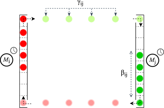
Figure 9: Interaction between two bittide machines, demonstrating the *FIFO and link action

The current occupancies of a machine’s buffers are used as a feedback signal to determine clock rate relative to its neighbours, and thus a clock control policy can be applied to take corrective action and stabilise the buffer occupancy within reasonable bounds. The control system is designed with the goal of preventing buffer overflow or underflow, but does not impact the logical synchrony property.

Various control policies may be valid for a given network topology, such as using a proportional controller [10], a proportional-integral controller [21], and a novel “reframing” controller [23]. Bidirectional links are not a hard requirement for clock control, but simplify analysis of control behaviour.

The free-running nature of bittide is that frames are assumed to always be in circulation. Unlike in the KPN model with blocking reads, a bittide system should not stall while awaiting a dependent signal. There must be sufficient initial frames, and thus sufficiently deep logical delays, such that the elastic buffer is never completely exhausted while awaiting inbound frames.

VI Finite FIFO Platforms

FFP[11] are a realisation of the KPN model, extended with blocking writes to prevent unbounded growth. A process can only fire if tokens are available for consumption at every input, and if there is space to emit tokens at every output. Otherwise it ‘stutters’, and skips that firing cycle. Figure 10 shows FFP with a single initial token.

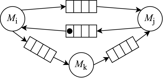
Figure 10: A three-machine *FFP where one token is placed in the unit delay buffer to ensure liveness

As a skipped cycle does not affect the semantics of KPN, it is acceptable to stutter at any time. Just as in the pure KPN model, $\lambda_{p\rightarrow{q}}$ is determined by the number of initial tokens from $p$ to $q$.

In this approach, buffer boundedness is enforced by locating the intermediate buffer on the receiver side of any communication channel. Blocking reads are trivial to implement by checking the local buffer occupancy. Blocking writes are enforced by using a heuristic to estimate remote buffer occupancy, which is always a conservative estimate.

VI-A Efficient Fullness Checking

Consider that the real occupancy of any buffer $\beta_{true}(t)$ at any time $t$ is equal to the number of tokens that have arrived over the link from a producer $p$, minus the number consumed at $q$, plus the initial occupancy:

$$\beta_{true}(t)=\theta_{p}(t-l_{pq})-\theta_{q}(t)+\beta(0)$$ (10)

The producer $p$ cannot know the current value of $\theta_{q}(t)$ nor the number of its own tokens that have reached the remote buffer $\theta_{p}(t-l_{pq})$. To provide this information, we include an unbuffered reverse link from consumer to producer. Figure 11 demonstrates this arrangement.

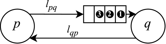
Figure 11: A buffered communication link from producer $p$ to consumer $q$, with a back-pressure link from $q$ to $p$

Over this reverse link $p$ measures the delayed firing count $\theta_{q}(t-l_{qp})$. $p$ can also measure its own current firing count $\theta_{p}(t)$. The difference between these two counts implies that absolute worst-case number of tokens that may still be in transit between the two machines, thus by substituting both of these into Equation 10:

$$\begin{gathered}\theta_{p}(t)\geq\theta_{p}(t-l_{pq})\\ \text{and }\theta_{q}(t-l_{qp})\leq\theta_{q}(t)\\ \therefore\beta_{true}(t)\leq\theta_{p}(t)-\theta_{q}(t-l_{qp})+\beta(0)\end{gathered}$$ (11)

Thus we can define a fullness checking function at $p$ which always gives a conservative occupancy estimate. This flow is given by the sequence diagram shown in Figure 12.

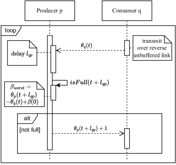
Figure 12: Sequence of isFull() *FFP behaviour

The overestimation error is proportional to the latency, thus the utilisation of the buffer will on average be less than the full capacity, and throughput degradation may occur correspondingly.

VI-B Modified FFPs for enhanced throughput

One limitation of the FFP model is that our performance degrades as we introduce communication delay, because the tokens required to progress spend some time in-flight. If a system has more initial tokens in circulation, processes can execute more often as the in-flight tokens begin to form a pipeline. At some token count we reach a saturation the throughput does not increase with additional tokens because the communication link is fully populated with in-flight tokens.

Such is the case in the bittide model, where the link is assumed to always be fully populated. As a result, a bittide system may have large logical delays ($\lambda$), but no blocking is required while awaiting inputs. Here we take inspiration from the delay masking of the bittide model and apply it to the FFP model, and introduce a special class of FFP which we denote as LSFP:

Definition 5.

LSFP is a special case of FFP where the initial marking in each buffer is governed by a heuristic, which is utilised for enhanced throughput as follows:

• For an edge $(\mathscr{M}_{i},\mathscr{M}_{j})\in E$ with some transmission time $l_{i\rightarrow j}$ and a consumer frequency $\omega_{j}$, the initial occupancy $\beta_{i\rightarrow j}(0)=\frac{l_{i\rightarrow j}}{\omega_{j}}$

Intuitively, the nominal frequency of the consumer process is the fastest rate of token consumption, which in turn governs the required spacing of in-flight tokens. Finding the true smallest marking resulting in maximum network performance is a special case of a maximum-flow circulation problem [24], which is NP-hard.

The increase in throughput as token count increases is demonstrated for illustrative purposes in Figure 13 for a simulated FFP. This topology was selected arbitrarily, but the expected trend is not topology-specific. Note that the physical response time is not meaningfully worsened until after the saturation point.

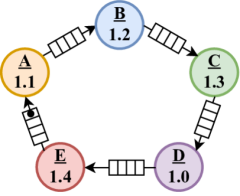
(a) *FFP with initial marking from $E{\rightarrow}A$

(b) Firing rate in blue (higher is better) and latency in red (lower is better) versus initial marking

Figure 13: A ring *FFP network. Nominal execution times labelled on each machine. A communication delay of 2.0 seconds has been added between machines

Now, each process becomes much closer to free-running execution. Consequently, predictable execution is gained with minimal impact to efficiency. These logical delays may be used in interesting ways at an application level, discussed in future works.

VII Implementation Comparison

Both the LSFP and bittide implementations are very similar in principle. Both are Kahn-like token pushing systems with intermediate FIFO buffers. The main difference is the clock control policy, which for LSFP is the use of blocking and in bittide is a novel clock control system based on backpressure. Here we briefly compare their runtime behaviour. We consider the LSN shown in Figure 14 implemented over both LSFP and bittide. This topology is arbitrarily chosen, but the clock behaviours are indicative for other topologies also. These results are generated using simulation, and are illustrative of the typical execution characteristics of each platform rather than providing a concrete benchmark.

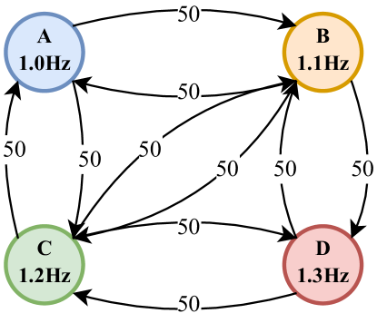
Figure 14: *LSN example topology for simulations. The nominal/initial frequency of each machine is annotated.

VII-A Throughput

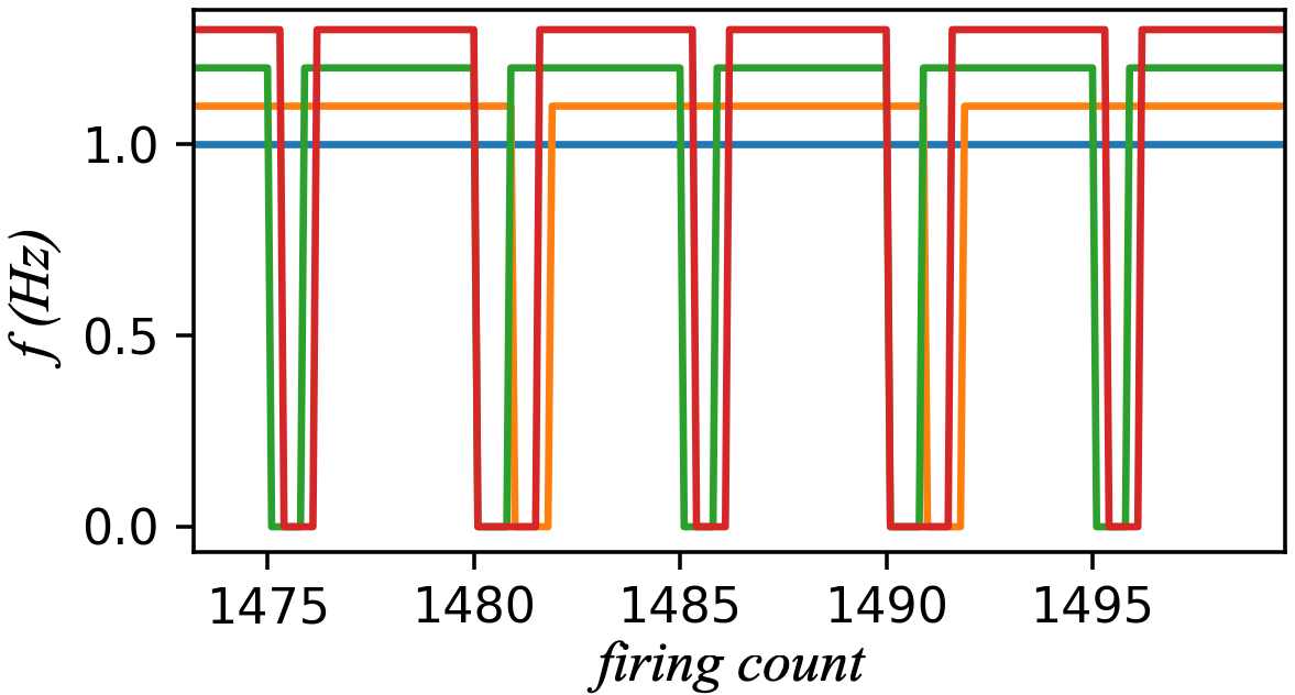
(a) *LSFP

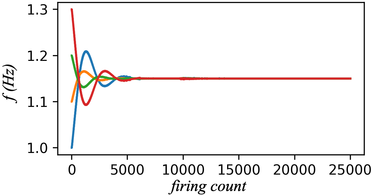
(b) bittide

Figure 15: Comparison of *LSFP and bittide tick/firing rate on a fully-connected four-machine network. Each coloured line represents a unique machine clock.

In this context, throughput describes the average logical tick frequency of each machine in the system. For our example topology, Figure 15 shows the frequency of each local clock evolves during the execution.

For the LSFP implementation (Figure 15(a)), the flow of tokens is limited by the slowest machine in the system. The slowest machine can remain free running, while the others must ‘stutter’ to modulate to the same value as the slowest machine on average. In contrast, the bittide proportional-integral controller (Figure 15(b)) converges all machine frequencies near the midpoint without ever blocking. In systems where task speed-up is possible, the bittide approach may have superior peak throughput. When task rates are very close to begin with, the throughput will be similar for both implementations.

Note that logical synchrony is still preserved during the transient or other instability as long as no frame data is lost due to overflow.

Observation 6.

Every machine in LSFP or bittide network must have the same average firing rate.

Due to FIFO bounds, for each producer-consumer pair the average rate of production must be the same as the average rate of consumption, barring some small initial difference before a steady-state is reached. If rates were unequal, FIFO would experience unbounded growth or loss during an extended execution and cause overflow.

VII-B Physical Latency

Physical-time delay between machines is entirely distinct to the logical delays discussed previously. These are related here by implementation, but this is not a hard requirement of the LSN definition.

The communication latency $\tau_{i\rightarrow{}j}(t)$ denotes the time elapsed between a production at $\theta_{i}(t){=}s$ and its consumption at $\theta_{j}(t{+}\tau_{i\rightarrow{}j}(t)){=}s{+}\lambda_{i\rightarrow{j}}$. This is not equivalent to transmission delay $l$ alone, because the token will be held in the recipient buffer for some time.

Observation 7.

The latency $\tau_{i\rightarrow{}j}(t)$ between two machines consists of the transmission delay and buffer propagation time

$$\tau_{i\rightarrow{}j}(t)\approx l_{ij}+\frac{\beta_{i\rightarrow{j}}(t)}{\omega_{j}(t)}$$ (12)

Note the implicit assumption that receiver frequency does not vary much during transmission. Because transmission delay is common to the latency for both implementations, we will compare just the buffer occupancy behaviour of each. Figure 16 shows each communication channel’s buffer occupancies for the bittide and LSFP example during a slice of execution.

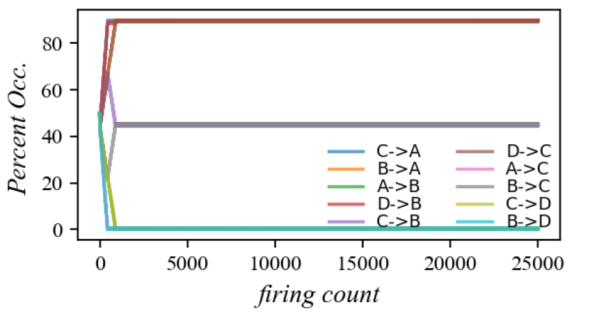
(a) *LSFP

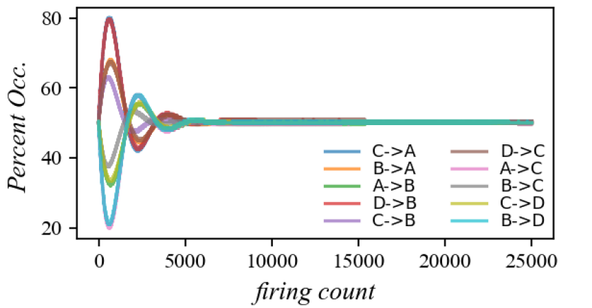
(b) bittide

Figure 16: Comparison of *LSFP and bittide channel buffer occupancy on a fully-connected four-machine network. Each coloured line represents a single channel.

Due to the clock controller, bittide buffers tend towards their initial occupancy. As a result, each bittide channel will (at steady state) have approximately the same latency at

$$\tau^{bt}_{i\rightarrow{}j}(t)\approx l_{ij}+\frac{\beta_{i\rightarrow{j}}^{max}}{2\omega_{j}(t)}$$ (13)

This is because $\beta_{i\rightarrow{j}}(t)$ from Equation 12 will evaluate to the buffer midpoint $\beta_{i\rightarrow{j}}^{max}/2$ at steady-state.

In contrast, in LSFP a buffer from a slower node to a faster node will tend to be near-empty and a buffer from a faster node to a slower node will tend to fill up before the skipping action kicks in. Note that the fast-to-slow link $D\rightarrow B$ in the simulation has a high occupancy, and the slow-to-fast link $B\rightarrow D$ has an almost-zero occupancy at all times. Consequently, links which end up empty will have shorter latencies than those which end up full :

$$l_{ij}\lessapprox\tau^{ffp}_{i\rightarrow{}j}(t)\lessapprox l_{ij}+\frac{\beta_{i\rightarrow{j}}^{max}}{\omega_{j}(t)}$$ (14)

VII-C Discussion

When comparing the two platforms as LSN implementations, the more advanced clock control mechanism of the bittide approach tends to improve throughput and make latency more consistent (after a transient period) compared to a blocking LSFP approach. Figure 15 and Figure 16 are generated from a specific topology, but the nature of the graphs is invariant to the topology given that a stable bittide controller exists. Thus, we demonstrate the key benefits of the decoupled elastic buffer MoC over blocking approaches, for the first time.

This is not entirely surprising given that we implicitly presented the assumption in these results that bittide clocks can increase in speed. Even if we remove this assumption and make the control one-sided (we cannot exceed the initial frequency), then clocks would be expected to settle at the rate of the slowest machine, as is the case in LSFP. The benefits to latency and jitter would still be present however, as the system would remain blocking-free.

However, a major redeeming property of LSFP is that the governing blocking mechanism can be implemented over many generic hardware platforms. In contrast, the dynamic clock control of bittide systems poses a reasonable implementation hurdle, and we generally assume that it remains a physical-layer protocol for bespoke hardware. This does not preclude the possibility that bittide-like control could be implemented at a more abstract software level. FIFO

VIII Conclusion

This paper addresses a gap of realisable formal models that preserve determinism and free running behaviour in distributed systems. We formalise a distributed network of machines as LSN. LSN provide a synchronous abstraction of a distributed system. We show that KPN, and their implementation as LSFP, preserve the LSN model. Subsequently, we show that the bittide protocol for distributed systems also preserves the LSN model. Thus, LSFP and bittide offer two distinct ways of realising LSN behaviour. We observe that in both LSFP and bittide, the Kahn-reminiscent effect of pipelining via buffers is used to achieve a greater overall throughput compared to signalling approaches used in GALS models, while preserving determinism, which is difficult to achieve over GALS. However, we also show that the decoupling of execution from synchronisation, in bittide leads to higher performance.

While this paper paves the way for formalising distributed synchronous systems using LSN, we have several avenues for future research. Firstly, we need to consider the design of application models which leverage logical synchrony. There is scope for introducing novel constructs into imperative synchronous languages which enable the seamless distribution of programs over bittide-like platforms. Moreover, precise delays expressed in logical-time have implications for efficient dataflow scheduling.

Logan Kenwright is a PhD student under Partha Roop at the University of Auckland. He holds a BE degree in Computer Systems Engineering with first-class honours from the University of Auckland. Logan’s research interests include programming models for synchronous and deterministic systems.

Partha Roop is a Professor and Associate Dean International of the Faculty of Engineering, The University of Auckland. Partha’s research interests are Formal Methods for Safety-Critical Software, AI and Machine Learning especially focussing on safety, and Real-Time Systems. He is a steering committee member of IEEE/ACM International Conference on Formal Methods and Models of Codesign (MEMOCOE) and an Associate Editor of IEEE Embedded Systems Letters. Recently, Partha is involved in the global partnership on AI for future pandemic resilience (gpai.ai).

Nathan Allen is a Research Fellow in the Department of Electrical, Computer, and Software Engineering at The University of Auckland. He received a B.E. (Hons) degree in Computer Systems Engineering in 2015, and a Ph.D. in Computer Systems Engineering in 2021, both from the University of Auckland, New Zealand. His research interests are in synchronous programming languages, formal methods, and embedded systems, which were all applied to the design of biomedical embedded systems in his Ph.D. research, and subsequently to the use of Spiking Neural Networks in robotic applications.

Călin Caşcaval (Fellow, IEEE) is Director of Engineering at Google Research, leading research in scalable distributed systems and compilers. He holds MS degrees from Technical University of Cluj, Romania and West Virginia University, USA, and in 2000 received a Ph. D. degree in Computer Science from University of Illinois at Urbana-Champaign. Călin spent his career in industrial research, where identified industry trends, defined, built, and delivered first of a kind prototypes and products, including: the first programmable networking (P4) production compiler and networking stack at Barefoot Networks; the first mobile heterogeneous computing runtime and parallel browser, mobile optimized math libraries and power optimization framework at Qualcomm Research; system software for the Blue Gene family of supercomputers and the first UPC compiler to scale to hundreds of thousands of processors at the IBM TJ Watson Research Center.

Sanjay Lall (Fellow, IEEE) is Professor of Electrical Engineering in the Information Systems Laboratory at Stanford University. He received a B.A. degree in Mathematics with first-class honors in 1990 and a Ph.D. degree in Engineering in 1995, both from the University of Cambridge, England. His research group focuses on algorithms for control, optimization, and machine learning. From 2018 to 2019 he was Director in the Autonomous Systems Group at Apple. Before joining Stanford he was a Research Fellow at the California Institute of Technology in the Department of Control and Dynamical Systems, and prior to that he was a NATO Research Fellow at Massachusetts Institute of Technology, in the Laboratory for Information and Decision Systems. He was also a visiting scholar at Lund Institute of Technology in the Department of Automatic Control. He has significant industrial experience applying advanced algorithms to problems including satellite systems, advanced audio systems, Formula 1 racing, the America’s cup, cloud services monitoring, and integrated circuit diagnostic systems. He is currently a visiting researcher at Google.

Tammo Spalink was born in Germany but mostly grew up in the USA.  He holds a BS degree from Carnegie Mellon University, an MS degree from the University of Arizona, and a PhD from Princeton University – all in Computer Science.  Tammo has spent his career to date at Alphabet where he has contributed to Android, ChromeOS, Loon, and numerous internal projects.  Tammo is currently an Engineering Director in Google Research responsible for a range of projects from silicon design to machine learning compilation.

Martin Izzard grew up in Durban, South Africa and was awarded BSEE and MSEE degrees from Natal University (today the University of KwaZulu-Natal). He completed a PhD at Trinity College Cambridge and was also awarded a Title A Fellowship at Trinity. He was at Texas Instruments in Dallas Texas for 21 years, starting in research and then holding a variety of technical- and general-management roles in both the digital and analog divisions of TI. He co-founded an Ethernet Switch chip company in 2017. He joined Google in 2019 as a research director.

References

- [1] Sanjay Lall, Calin Cascaval, Martin Izzard, and Tammo Spalink. Logical synchrony and the bittide mechanism. arXiv preprint arXiv:2308.00144, 2023.
- [2] Edward A Lee and Alberto Sangiovanni-Vincentelli. A framework for comparing models of computation. IEEE Transactions on computer-aided design of integrated circuits and systems, 17(12):1217–1229, 1998.
- [3] Charles Antony Richard Hoare et al. Communicating sequential processes, volume 178. Prentice-hall Englewood Cliffs, 1985.
- [4] Robin Milner. Communication and concurrency, volume 84. Prentice hall Englewood Cliffs, 1989.
- [5] Gul Agha. Actors: a model of concurrent computation in distributed systems. MIT press, 1986.
- [6] KAHN Gilles. The semantics of a simple language for parallel programming. Information processing, 74:471–475, 1974.
- [7] A. Benveniste, P. Caspi, S.A. Edwards, N. Halbwachs, P. Le Guernic, and R. De Simone. The synchronous languages 12 years later. Proceedings of the IEEE, 91(1):64–83, January 2003.
- [8] Stephen Edwards, Luciano Lavagno, Edward A Lee, and Alberto Sangiovanni-Vincentelli. Design of embedded systems: Formal models, validation, and synthesis. Proceedings of the IEEE, 85(3):366–390, 1997.
- [9] Reinhard Maier, Günther Bauer, Georg Stöger, and Stefan Poledna. Time-triggered architecture: A consistent computing platform. IEEE Micro, 22(4):36–45, 2002. Publisher: IEEE.
- [10] Sanjay Lall, Calin Cascaval, Martin Izzard, and Tammo Spalink. Modeling and Control of Google bittide Synchronization. arXiv preprint arXiv:2109.14111, 2021.
- [11] Stavros Tripakis, Claudio Pinello, Albert Benveniste, Alberto Sangiovanni-Vincentelli, Paul Caspi, and Marco Di Natale. Implementing synchronous models on loosely time triggered architectures. IEEE Transactions on Computers, 57(10):1300–1314, 2008. Publisher: IEEE.
- [12] Hermann Kopetz and Günther Bauer. The time-triggered architecture. Proceedings of the IEEE, 91(1):112–126, 2003.
- [13] Marten Lohstroh, Christian Menard, Soroush Bateni, and Edward A. Lee. Toward a lingua franca for deterministic concurrent systems. ACM Trans. Embed. Comput. Syst., 20(4), may 2021.
- [14] Patricia Derler, Thomas H Feng, Edward A Lee, Slobodan Matic, Hiren D Patel, Yang Zheo, and Jia Zou. Ptides: A programming model for distributed real-time embedded systems. Technical report, CALIFORNIA UNIV BERKELEY DEPT OF ELECTRICAL ENGINEERING AND COMPUTER SCIENCE, 2008.
- [15] Guillaume Baudart, Albert Benveniste, and Timothy Bourke. Loosely Time-Triggered Architectures: Improvements and Comparisons. ACM Transactions on Embedded Computing Systems, 15(4):1–26, September 2016.
- [16] Albert Benveniste, Benoit Caillaud, and Paul Le Guernic. From synchrony to asynchrony. In CONCUR’99 Concurrency Theory: 10th International Conference Eindhoven, The Netherlands, August 24—27, 1999 Proceedings 10, pages 162–177. Springer, 1999.
- [17] Paul Caspi, Alain Girault, and Daniel Pilaud. Automatic distribution of reactive systems for asynchronous networks of processors. IEEE Transactions on Software Engineering, 25(3):416–427, 1999.
- [18] Paul Le Guernic, Jean-Pierre Talpin, and Jean-Christophe Le Lann. Polychrony for system design. Journal of Circuits, Systems, and Computers, 12(03):261–303, 2003.
- [19] Stephen A Edwards. On determinism. Principles of Modeling: Essays Dedicated to Edward A. Lee on the Occasion of His 60th Birthday, pages 240–253, 2018.
- [20] Edward A Lee and Thomas M Parks. Dataflow process networks. Proceedings of the IEEE, 83(5):773–801, 1995.
- [21] Sanjay Lall, Calin Cascaval, Martin Izzard, and Tammo Spalink. Resistance Distance and Control Performance for Google bittide Synchronization. arXiv preprint arXiv:2111.05296, 2021.
- [22] Josep Carmona, Jordi Cortadella, Mike Kishinevsky, and Alexander Taubin. Elastic Circuits. IEEE Transactions on Computer-Aided Design of Integrated Circuits and Systems, 28(10):1437–1455, October 2009. Conference Name: IEEE Transactions on Computer-Aided Design of Integrated Circuits and Systems.
- [23] Sanjay Lall, Calin Cascaval, Martin Izzard, and Tammo Spalink. On buffer centering for bittide synchronization. arXiv preprint arXiv:2303.11467, 2023.
- [24] Ravindra K Ahuja, Thomas L Magnanti, and James B Orlin. Network flows. 1988.