Astronomy Letters, 2023, Vol. 49, No.11 Origin of the Near-Surface Shear Layer of Solar Rotation L. L. Kitchatinov^1,2* Sun: rotation – convection – turbulence Helioseismology has revealed an increase in the rotation rate with depth in a thin ($\sim$30 Mm) near-surface layer. The normalized rotational shear in this layer is independent of latitude. This rotational state is shown to be a consequence of the short characteristic time of near-surface convection compared to the rotation period, and the radial anisotropy of the convective turbulence. Analytical derivations within mean-field hydrodynamics reproduce the observed normalized rotational shear and are in agreement with numerical experiments on the radiative hydrodynamics of solar convection. The near-surface shear layer is the source of the global meridional flow important for the solar dynamo.

1 INTRODUCTION

Helioseismology has revealed a rapid increase in the rotation rate with depth just below the solar surface (Thompson et al. 1996; Schou et al. 1998). The near-surface shear layer (NSSL) is interesting per se and, as Brandenburg (2005) and Pipin & Kosovichev (2011) noted, may be important for the solar dynamo. The origin of the NSSL remains a significant problem in the theory of differential rotation.

Lebedinsky (1941) was probably the first to show that stellar convection, under the influence of the Coriolis force, can redistribute angular momentum along the stellar radius, producing differential rotation. This phenomenon has since been widely studied and confirmed in various astrophysical contexts. The angular momentum fluxes discovered by Lebedinsky are commonly referred to as the $\Lambda$-effect (Rüdiger 1989). The $\Lambda$-effect requires anisotropy of the turbulent mixing: the angular momentum flux is directed downwards in the radius if the mixing intensity along the radius is greater than along the longitude. This radial anisotropy can be a consequence of the radial direction of the buoyancy forces driving convection.

The explanation of the NSSL in terms of mean-field hydrodynamics seems obvious. The standard boundary conditions require that the angular momentum flux through the outer surface is zero. The downward flux due to the $\Lambda$-effect is then balanced by the transport in the opposite direction by the eddy viscosity, and the rotation rate increases with depth (Kitchatinov 2013). However, this is not a generally accepted explanation. Hotta et al. (2015) and Gunderson & Battacharjee (2019) suggested that the NSSL is produced by a large-scale meridional flow. Jha & Choudhuri (2021) thought that the NSSL is a consequence of the balance between the centrifugal and baroclinic forces.

It is noteworthy that although the radial rotational shear and the rotation rate decrease with latitude, the normalized shear

$$\frac{r}{\Omega}\frac{\partial\Omega}{\partial r}\simeq-1$$ (1)

is constant with latitude (Barekat et al. 2014). An adequate theory should explain this fact. In this paper we show that the absence of a latitudinal dependence of the normalized rotational shear is due to the short correlation time of the near-surface turbulence compared to the solar rotation period. This result follows from the general principles of the theory and does not depend on the (necessarily approximate) NSSL derivation method, although the normalized rotational shear value depends on the approximations of the theory. The quasi-linear approximation of mean-field hydrodynamics gives the shear value of Eq. (1) for the anisotropy of turbulence found in the numerical experiments of Kitiashvili et al. (2023).

The $\Lambda$-effect and eddy viscosities for anisotropic turbulence with a short correlation time are discussed in section 2. As we will see, the latitudinally constant normalized rotational shear in the NSSL in this case follows from the general structure of the Reynolds stress tensor. In section 3, the rotational shear in the near-surface layer is derived in the quasi-linear approximation for turbulence anisotropic in both velocity directions and shape of their correlation region (formulae for the $\Lambda$-effect and eddy viscosities are given in the Appendix). Section 4 summarizes the results and concludes.

2 GENERAL EXPRESSION FOR THE NEAR-SURFACE SHEAR

The effects of turbulence in mean-field hydrodynamics are accounted for by the Reynolds stress tensor

$$R_{ij}=-\rho\langle v_{i}v_{j}\rangle,$$ (2)

where $\rho$ is the density, $v$ is the fluctuating velocity ($\langle\mbox{\boldmath$v$}\rangle=0$), and the angular brackets denote an averaging. The contributions to the Reynolds stresses responsible for the $\Lambda$-effect ($R^{\Lambda}_{ij}$) and the eddy viscosities ($R^{\nu}_{ij}$) are distinguished in the problem of differential rotation:

$$R_{ij}=R^{\Lambda}_{ij}+R^{\nu}_{ij}.$$ (3)

To derive these contributions, the turbulent velocity $\mbox{\boldmath$v$}=\mbox{\boldmath$u$}+\mbox{\boldmath$u$}^{\prime}$ is divided into the perturbation $\mbox{\boldmath$u$}^{\prime}$ by the large-scale flow and the unperturbed ‘original’ part $u$. Then,

$$R_{ij}=-\rho\langle u^{\prime}_{i}u_{j}+u_{i}u^{\prime}_{j}\rangle.$$ (4)

The $\Lambda$-effect arises from the perturbations $\mbox{\boldmath$u$}^{\prime}$ caused by the Coriolis force in a reference frame rotating with a local angular velocity $\Omega$, while the eddy viscosities result from the perturbations by the inhomogeneous flow $V$ in this reference frame (Kitchatinov 2005).

For the perturbation by the Coriolis force we have the estimate:

$${\mbox{\boldmath$u$}}^{\prime}=2\tau\Omega\ {\mbox{\boldmath$u$}}\times\hat{\mbox{\boldmath$z$}},$$ (5)

where $\tau$ is the characteristic time scale of turbulent convection (correlation time) and $\hat{\mbox{\boldmath$z$}}$ is a unit vector along the rotation axis. Substituting (5) into (4) gives an expression for the cross-components

$$R^{\Lambda}_{r\varphi} = \rho\,2\tau\Omega\left(\langle u_{r}^{2}\rangle-\langle u_{\varphi}^{2}\rangle\right)\sin\theta,$$

$$R^{\Lambda}_{\theta\varphi} = \rho\,2\tau\Omega\left(\langle u_{\theta}^{2}\rangle-\langle u_{\varphi}^{2}\rangle\right)\cos\theta=0$$ (6)

of the stress tensor responsible for the angular momentum transport. Here we use the usual spherical coordinates ($r,\theta,\varphi$) and take into account that there is only radial anisotropy in direction of the (unit) vector $\hat{\mbox{\boldmath$r$}}=\mbox{\boldmath$r$}/r$ for the original turbulence:

$$\langle u_{i}u_{j}\rangle = \frac{1}{2}\left(\langle u^{2}\rangle-\langle u_{r}^{2}\rangle\right)\delta_{ij}$$ (7)

$$- \frac{1}{2}\left(\langle u^{2}\rangle-3\langle u_{r}^{2}\rangle\right)\hat{r}_{i}\hat{r}_{j}.$$

The estimations (5) and (6) are valid for small Coriolis number

$$\Omega^{*}=2\tau\Omega,$$ (8)

$\Omega^{*}\ll 1$. This number measures the intensity of the interaction between convection and rotation. The interaction is weak for small Coriolis number. This is why the small contribution $\langle u_{i}^{\prime}u_{j}^{\prime}\rangle$ is omitted in (4). The profile of the Coriolis number near the solar surface is shown in Fig. 1; the profile is estimated from the MESA model of stellar structure and evolution of Paxton et al. (2013) (version 496f408) applied to the Sun. The increase in $\Omega^{*}$ towards the surface at small depths is caused by the convection switch-off. MESA uses the rough mixing length approximation. The inhomogeneities in thermal diffusivity caused by partial ionization lead to preferential scales of solar granulation and supergranulation (Getling et al. 2013; Shcheritsa et al. 2018). Therefore, Fig. 1 also shows an estimate for solar granulation.

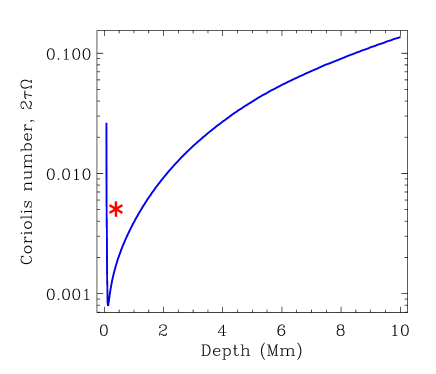
Figure 1: Coriolis number (8) versus depth beneath the solar surface. The asterisk indicates the estimate for the solar granulation.

The Figure covers the range of depths at which Barekat et al. (2014) found the rotational shear (1) in the NSSL seismologically. Of course, the NSSL does not extend to all depths. At a depth of about 30 000 km, the radial rotational shear changes its sign (Schou et al. 1989). As this depth is approached, the Coriolis number increases, the rotational shear decreases, and the relation (1) breaks down (Komm 2022; Antia & Basu 2022). In this paper we consider the NSSL region where Eq. (1) is valid.

As can be seen from Fig. 1, the Coriolis number near the surface is small. This greatly simplifies the theory of the near-surface layer: the theory can be linear in rotation rate. The estimates above have been made to demonstrate this fact. Let us now consider the general structure of the stress tensor for small Coriolis number.

The tensor $R^{\Lambda}_{ij}$ can be constructed from the angular velocity pseudovector $\Omega$, radial vector $\hat{\mbox{\boldmath$r$}}={\mbox{\boldmath$r$}}/r$ of anisotropy, and unitary symmetric ($\delta_{ij}$) and fully antisymmetric ($\varepsilon_{ijk}$) tensors. For the symmetric tensor $R^{\Lambda}_{ij}$ only the following structure linear in $\Omega$ is possible:

$$R^{\Lambda}_{ij}=-\rho\nu_{\Lambda}\left(\hat{r}_{i}\varepsilon_{jkl}+\hat{r}_{j}\varepsilon_{ikl}\right)\hat{r}_{k}\Omega_{l}\ ,$$ (9)

where $\nu_{\Lambda}$ is the yet undetermined constant with the dimension of viscosity and the repetition of subscripts means summation. There is no other way to construct the non-dissipative part of the Reynolds stresses linear in the angular velocity. For example, the cannot be a structure $\tilde{\nu}({\mbox{\boldmath$\Omega$}}\cdot\hat{\mbox{\boldmath$r$}})\hat{r}_{i}\hat{r}_{j}$ since the coefficient $\tilde{\nu}$ must be a pseudoscalar, which is only possible with the inclusion of the nonlinear contributions in $\Omega$. A standard order-of-magnitude estimate, $\nu_{\Lambda}\sim\tau u^{2}$, shows that Eq. (9) is linear in the Coriolis number.

In the deep convection zone, the Coriolis number is not small. The nonlinear theory in angular velocity should be applied there, which leads to a complication of the $\Lambda$-effect compared to Eq. (9) (Rüdiger et al. 2013).

The structure of the dissipative part $R^{\nu}_{ij}$ of the stress tensor is even easier to determine. Since the large-scale velocity $V$ can only enter via its spatial derivative,

$$R^{\nu}_{ij}=\rho{\cal N}_{ijkl}\frac{\partial V_{k}}{\partial r_{l}},$$ (10)

the viscosity tensor ${\cal N}_{ijkl}$ can be constructed from $\hat{\mbox{\boldmath$r$}}$ and $\delta_{ij}$ only:

$${\cal N}_{ijkl} = \nu_{1}(\delta_{ik}\delta_{jl}+\delta_{il}\delta_{jk})+\nu_{2}\delta_{ij}\delta_{kl}$$ (11)

$$+ \nu_{3}(\delta_{ik}\hat{r}_{j}\hat{r}_{l}+\delta_{jk}\hat{r}_{i}\hat{r}_{l})$$

$$+ \nu_{4}(\delta_{il}\hat{r}_{j}\hat{r}_{k}+\delta_{jl}\hat{r}_{i}\hat{r}_{k})$$

$$+ \nu_{5}\delta_{ij}\hat{r}_{k}\hat{r}_{l}+\nu_{6}\delta_{kl}\hat{r}_{i}\hat{r}_{j}+\nu_{7}\hat{r}_{i}\hat{r}_{j}\hat{r}_{k}\hat{r}_{l}.$$

The longitude-averaged velocity $V$ in the rotating frame of reference includes the differential rotation $\delta\Omega(r,\theta)$ and the axisymmetric meridional circulation.

The normalized rotational shear $\partial\ln(\Omega)/\partial\ln(r)$ near the surface can be expressed by the coefficients $\nu_{\Lambda}$ and $\nu_{1},...,\nu_{7}$ of (9) and (11). Some methods of the mean-field theory can be used to derive these coefficients. All of the known methods are approximate. However, whatever method is used, the calculations will result in a latitude independent normalized rotational shear. This assertion follows from the condition

$$R_{r\varphi}=R^{\Lambda}_{r\varphi}+R^{\nu}_{r\varphi}=0$$ (12)

at the surface of the convection zone. Note that $R_{r\varphi}$ is the surface density of the azimuthal force acting on an area normal to the radius $r$. The boundary condition (12) requires that the surface density of the external forces to be zero. Condition (12) means that the global flow is controlled by internal processes in the Sun, not by an external forcing.

Taking into account equations (9) to (11), condition (12) gives

$$R_{r\varphi}=\rho\,\sin\theta\left(\nu_{\Lambda}\Omega+(\nu_{1}+\nu_{3})r\frac{\partial\Omega}{\partial r}\right)=0.$$ (13)

Here, we take into account that the mean flow is axially symmetric about the rotation axis and that the Reynolds stresses for a fixed point ($r,\theta$) are defined in the coordinate system rotating with a local angular velocity $\Omega(r,\theta)$. Therefore, the velocity $V$ in (10) includes only the rotational shear and meridional circulation, which, however, does not contribute to $R_{r,\varphi}$ of Eq. (13).

The equation for the near-surface normalized rotational shear,

$$\frac{r}{\Omega}\frac{\partial\Omega}{\partial r}=-\frac{\nu_{\Lambda}}{\nu_{1}+\nu_{3}},$$ (14)

common to all methods of mean-field hydrodynamics, follows from Eq. (13). In agreement with helioseismology, the normalized rotational shear (14) does not depend on latitude. However, this latitude-independent constant depends on the (necessarily approximate) method of its derivation. The normalized rotational shear value (1) of Barekat et al. (2014) can be reproduced using the quasi-linear approximation of mean-field hydrodynamics.

3 QUASI-LINER APPROXIMATION

In the quasi-linear approximation, the disturbances $\mbox{\boldmath$u$}^{\prime}$ of the turbulent velocity $u$ in Eq. (4) can be obtained from a linearized equation (see, e.g., Rüdiger et al. 2013). It is convenient to use the Fourier transform,

$$\hat{\mbox{\boldmath$u$}}({\mbox{\boldmath$k$}},\omega)=\frac{1}{(2\pi)^{4}}\int{\mbox{\boldmath$u$}}({\mbox{\boldmath$r$}},t)\exp(\mathrm{i}\omega t-\mathrm{i}{\mbox{\boldmath$k$}}\cdot{\mbox{\boldmath$r$}})\mathrm{d}^{3}{\mbox{\boldmath$r$}}\,\mathrm{d}t,$$ (15)

which converts the differentiation operators into algebraic ones:

$$(\nu k^{2}-\mathrm{i}\omega)\hat{u}^{\prime}_{i}({\mbox{\boldmath$k$}},\omega)=-2\varepsilon_{inm}\hat{k}_{n}\hat{u}_{m}({\mbox{\boldmath$k$}},\omega)(\hat{\mbox{\boldmath$k$}}\cdot{\mbox{\boldmath$\Omega$}})$$

$$-\mathrm{i}(\delta_{in}-\hat{k}_{i}\hat{k}_{n})k_{m}\int{\large[}\hat{u}_{m}({\mbox{\boldmath$k$}}-{\mbox{\boldmath$k$}}^{\prime},\omega-\omega^{\prime})\hat{V}_{n}(\mbox{\boldmath$k$}^{\prime},\omega^{\prime})$$

$$+\,\hat{u}_{n}({\mbox{\boldmath$k$}}-{\mbox{\boldmath$k$}}^{\prime},\omega-\omega^{\prime})\hat{V}_{m}(\mbox{\boldmath$k$}^{\prime},\omega^{\prime}){\large]}\,\mathrm{d}{\mbox{\boldmath$k$}}^{\prime}\mathrm{d}\omega^{\prime}.$$ (16)

In this equation, $\hat{\mbox{\boldmath$k$}}={\mbox{\boldmath$k$}}/k$ is a unit vector and the incompressibility condition, $\mbox{\boldmath$k$}\cdot\hat{\mbox{\boldmath$u$}}$ = 0, has been used to eliminate pressure.

To derive the stress tensor (4), Eq. (16) is multiplied by $\hat{u}_{j}$, then averaged, inverse Fourier transformed, and the expression with transposed indices $i$ and $j$ is added for symmetry. The derivations are limited to the linear approximation in the small parameter $k^{\prime}/k\ll 1$ (the ratio of the correlation length to the spatial scale of the mean velocity $V$). The first term on the right-hand side of Eq. (16) then gives the $\Lambda$-effect and the rest give the eddy viscosities.

To perform the derivations, we need the spectral tensor $\hat{Q}_{ij}(k,\omega)$ for the original turbulence with radial anisotropy

$$\langle\hat{u}_{i}({\mbox{\boldmath$k$}},\omega)\hat{u}_{j}({\mbox{\boldmath$k$}}_{1},\omega_{1})\rangle=\hat{Q}_{ij}({\mbox{\boldmath$k$}},\omega)\delta({\mbox{\boldmath$k$}}+{\mbox{\boldmath$k$}}_{1})\delta(\omega+\omega_{1}),$$

$$\hat{Q}_{ij}({\mbox{\boldmath$k$}},\omega)=\frac{E(k,\omega,\mu)}{16\pi k^{2}}\large[(1+S)(\delta_{ij}-\hat{k}_{i}\hat{k}_{j})$$

$$\hskip 22.76228pt-\,S(\mu^{2}\delta_{ij}+\hat{r}_{i}\hat{r}_{j}-\mu\,\hat{r}_{i}\hat{k}_{j}-\mu\,\hat{r}_{j}\hat{k}_{i})\large],$$ (17)

where $\mu=\hat{\mbox{\boldmath$r$}}\cdot\hat{\mbox{\boldmath$k$}}=\cos({\mbox{\boldmath$r$}}\wedge{\mbox{\boldmath$k$}})$ is the cosine of the angle between the vectors $r$ and $k$. Equation (17) allows for two types of anisotropy: anisotropy of directions and anisotropy of the shape of the correlation region of the fluctuating velocity $u$. The parameter $S$ defines the directional anisotropy of the velocity. For $S=0$ the distribution of the velocity direction is isotropic, but the dependence of the spectral function $E$ on $\mu$ accounts for the anisotropy of the correlation region. For $\partial^{2}E/\partial\mu^{2}>0$, the radial correlation scale is smaller than the horizontal correlation scale (oblate convective cells). For $\partial^{2}E/\partial\mu^{2}<0$, the correlation region is prolate in radius. If $\partial E/\partial\mu=0$, there is no shape anisotropy, but the directional anisotropy may be present: $\langle u^{2}_{r}\rangle>\langle u^{2}\rangle/3$ for $S<0$ (radial type anisotropy) and $\langle u^{2}_{r}\rangle<\langle u^{2}\rangle/3$ for $S>0$ (horizontal anisotropy).

Equation (17) for the original turbulence differs from the one used previously (Kitchatinov 2016a) by allowing for the shape anisotropy. As before, the positive definiteness of the spectral tensor imposes the inequality

$$S\geq-1\,.$$ (18)

This implies that the turbulence cannot consist of radial flows only. For maximum radial anisotropy ($S=-1$) there are horizontal flows with $\langle u^{2}\rangle-\langle u^{2}_{r}\rangle>0$. However, the maximum value of S is not bounded, and (two-dimensional) turbulence with $u_{r}=0$ is possible. Note that if the fluctuation spectrum $E(k,\omega)$ does not depend on $\mu$ (there is no shape anisotropy), the following simple expression for the parameter $S$ in terms of the rms velocities holds:

$$S={\langle u^{2}\rangle}/{\langle u^{2}_{r}\rangle}-3.$$ (19)

The eddy viscosities and the coefficient $\nu_{\Lambda}$ of Eq. (9) for the $\Lambda$-effect, calculated in the quasilinear approximation for the turbulence model (17) are given in the Appendix. Substitution of the transport coefficients in Eq. (14) gives

$$\frac{r}{\Omega}\frac{\partial\Omega}{\partial r}=\frac{S\int\limits_{0}^{\infty}\int\limits_{0}^{\infty}\frac{\nu k^{2}}{\nu^{2}k^{4}+\omega^{2}}\int\limits_{0}^{1}E(k,\omega,\mu)(1-\mu^{2})^{2}\mathrm{d}\mu\,\mathrm{d}k\mathrm{d}\omega}{4\int\limits_{0}^{\infty}\int\limits_{0}^{\infty}\frac{\nu^{3}k^{6}}{(\nu^{2}k^{4}+\omega^{2})^{2}}\int\limits_{0}^{1}E(k,\omega,\mu)\mu^{2}(1-\mu^{2})\mathrm{d}\mu\,\mathrm{d}k\mathrm{d}\omega}.$$ (20)

According to this equation, the normalized near-surface shear is proportional to the anisotropy parameter $S$. The rotation rate increases with depth for the radial anisotropy ($S<0$), as it must be the case (Lebedinsky 1941). Note that the rotational shear is caused by the directional anisotropy of the turbulent velocity. The shape anisotropy alone does not give such a shear.

Estimating the rotational shear requires a further simplification of Eq. (19). The so-called $\tau$-approximation (Brandenburg & Subramanian 2005) can be used for this purpose. The coefficient $\nu k^{2}-{\mathrm{i}}\omega$ on the left side of Eq. (16) is replaced by the inverse correlation time $1/\tau$. In the final result (20) of our quasilinear derivations, such a replacement can be done by setting $\nu k^{2}=\tau^{-1}$ and $\omega=0$. Also neglecting the shape anisotropy (the spectrum $E(k,\omega)$ does not depend on $\mu$), we obtain a simple expression for the normalized rotational shear:

$$\frac{r}{\Omega}\frac{\partial\Omega}{\partial r}=S.$$ (21)

According to Eq. (18), the shear value (1) measured by helioseismology is reproduced with the maximum possible radial anisotropy. The maximum anisotropy may be a consequence of the extreme anisotropy of the driving convection buoyancy forces which point up or down in radius.

Note that the normalized rotational shear (21) does not depend on the intensity of the turbulence (provided that the Coriolis number remains small). This is already clear from the general expression (14) for the shear. Only the anisotropy of convective turbulence, not its intensity, is important for the differential rotation in the NSSL.

4 DISCUSSION AND CONCLUSIONS

The proposed theory explains the NSSL in terms of the anisotropy of near-surface turbulent convection under the condition (12) of zero surface density of external forces. Radial anisotropy with a negative parameter $S$ (19) corresponds to the observed increase in the rotation rate with depth. In this case, the downward non-dissipative flux of the angular momentum ($\Lambda$-effect) is balanced by the counteracting viscous flux. For small Coriolis number (Fig. 1), the normalized rotational shear (14) is constant with latitude, regardless of the theoretical method used for its derivation. The quasi-linear approximation of the mean-field theory reproduces the shear value (1) measured by helioseismology for the maximum radial anisotropy with $S=-1$.

This explanation is consistent with the numerical experiments of Kitiashvili et al. (2023), whose 3D radiative hydrodynamic simulations reproduced the NSSL. The cross component $R_{xz}$ of the stress tensor ($R_{r\varphi}$ in the notation of this paper) in their computations is small compared to the diagonal components, in accordance with condition (12) of this paper. Kitiashvili et al. (2023) also gave the anisotropy of the simulated convective turbulence. They used the anisotropy parameter

$$A_{V}=1-3\langle u_{z}^{2}\rangle/\langle u^{2}\rangle$$ (22)

which was almost constant with the value of $A_{V}\simeq-0.5$ inside the convection zone (see Fig. 4 in Kitiashvili et al. 2023). A negative $A_{V}$ means radial anisotropy. The parameter $A_{V}$ (22) can be converted into the parameter $S$ (19) of this paper,

$$S=3A_{V}/(1-A_{V}).$$ (23)

For $A_{V}\simeq-0.5$ this gives $S\simeq-1$, for which our derivations reproduce the normalized rotational shear value (1) detected by helioseismology.

The anisotropy of the turbulence could be inferred from the observations of photospheric convection (see, e.g., Lida et al. 2010; Abramenko et al. 2013; Yelles Chaouche et al. 2020). The observations clearly show the presence of radial flows in the photosphere. However, since different velocity components are measured by different methods (the Doppler measurements along the line of sight and the motion of tracers in horizontal directions), it is difficult to infer the anisotropy from the observations.

The importance of the NSSL for the solar dynamo is related in particular to the fact that the global meridional flow is excited in the surface layer. The meridional circulation most likely determines the period of the solar cycle and it is responsible for the equatorward migration of sunspots (see, e.g., the review by Hazra et al. 2023). Condition (12) disturbs the balance between the centrifugal and baroclinic forces, and this imbalance drives the meridional circulation (Kitchatinov 2016b).

Models of large-scale flows in the Sun and stars place the upper boundary at a few percent of the radius below the photosphere to avoid numerical difficulties with sharp near-surface stratification. The boundary conditions in mean-field models set the radial component of the large-scale flow to be zero, $V_{r}=0$, but the finite turbulent velocities $u_{r}$ at the upper boundary are included via the condition (12) for the Reynolds stresses. In this case, it is possible to reproduce the increase in the rotation rate with depth in about the lower third of the NSSL and the global meridional flow (Kitchatinov & Olemskoy 2011). A different approach is used in the 3D numerical models of large-scale convection. Here, the zero radial velocity, $v_{r}=0$, is used as a boundary condition without separation in its large-scale and turbulent components. This excludes the $\Lambda$-effect of the Reynolds stress (12).This can lead to difficulties in reproducing the NSSL and the global meridional circulation in 3D numerical simulations of large-scale convection.

Our main conclusions can be formulated as follows

• The near-surface rotational shear in the Sun is a consequence of the balance between the $\Lambda$-effect and eddy viscosity for anisotropic turbulent convection.

• The normalized rotational shear near the solar surface does not depend on latitude because the characteristic time of turbulent convection is here short compared to the rotation period. As a consequence, the $\Lambda$-effect redistributes the angular momentum in radius only, but not in the latitude.

• The quasi-linear approximation of mean-field hydrodynamics reproduces the rotational shear in the NSSL measured by helioseismology with the turbulence anisotropy value found in the numerical radiative hydrodynamics experiments.

APPENDIX: Effective transport coefficients for anisotropic turbulence

In this Appendix, turbulent transport coefficients for the turbulence model of Eq. (17) are given. The coefficient $\nu_{\Lambda}$ of the $\Lambda$-effect (9) reads

$$\nu_{\Lambda} = -\frac{S}{2}\int\limits_{0}^{\infty}\int\limits_{0}^{\infty}\frac{\nu k^{2}}{\nu^{2}k^{4}+\omega^{2}}$$ (24)

$$\times \int\limits_{0}^{1}E(k,\omega,\mu)(1-\mu^{2})^{2}\mathrm{d}\mu\,\mathrm{d}k\mathrm{d}\omega.$$

For the eddy viscosities of Eq. (11) we find

$$\nu_{1} = \frac{1}{4}\int\limits_{0}^{\infty}\int\limits_{0}^{\infty}\frac{\nu k^{2}}{\nu^{2}k^{4}+\omega^{2}}\int\limits_{0}^{1}E(k,\omega,\mu)$$ (25)

$$\times\Bigg{[}\mu^{2}(1+\mu^{2})+S\mu^{2}(1-\mu^{2})$$

$$+ \frac{\nu^{2}k^{4}-\omega^{2}}{\nu^{2}k^{4}+\omega^{2}}(1+S)(1-\mu^{2})^{2}\Bigg{]}\mathrm{d}\mu\,\mathrm{d}k\mathrm{d}\omega,$$

$$\nu_{2} = \frac{1}{4}\int\limits_{0}^{\infty}\int\limits_{0}^{\infty}\frac{\nu k^{2}}{\nu^{2}k^{4}+\omega^{2}}\int\limits_{0}^{1}E(k,\omega,\mu)\Bigg{[}3+\mu^{4}$$ (26)

$$+ S(1-\mu^{2})(3-\mu^{2})-\frac{\nu^{2}k^{4}-\omega^{2}}{\nu^{2}k^{4}+\omega^{2}}$$

$$\times(1-\mu^{2})\left(3+\mu^{2}+3S(1-\mu^{2})\right)\Bigg{]}\mathrm{d}\mu\,\mathrm{d}k\mathrm{d}\omega,$$

$$\nu_{3} = \frac{1}{4}\int\limits_{0}^{\infty}\int\limits_{0}^{\infty}\frac{\nu k^{2}}{\nu^{2}k^{4}+\omega^{2}}\int\limits_{0}^{1}E(k,\omega,\mu)\Bigg{[}3\mu^{2}-5\mu^{4}$$ (27)

$$- S\mu^{2}(1-\mu^{2})+\frac{\nu^{2}k^{4}-\omega^{2}}{\nu^{2}k^{4}+\omega^{2}}$$

$$\times(1-\mu^{2})\left(5\mu^{2}-1-S(1-\mu^{2})\right)\Bigg{]}\mathrm{d}\mu\,\mathrm{d}k\mathrm{d}\omega,$$

$$\nu_{4} = \frac{1}{4}\int\limits_{0}^{\infty}\int\limits_{0}^{\infty}\frac{\nu k^{2}}{\nu^{2}k^{4}+\omega^{2}}\int\limits_{0}^{1}E(k,\omega,\mu)\Bigg{[}1-5\mu^{4}$$ (28)

$$+ S(1-\mu^{2})(1-3\mu^{2})-\frac{\nu^{2}k^{4}-\omega^{2}}{\nu^{2}k^{4}+\omega^{2}}$$

$$\times(1-\mu^{2})\left(1-5\mu^{2}+S(1-\mu^{2})\right)\Bigg{]}\mathrm{d}\mu\,\mathrm{d}k\mathrm{d}\omega,$$

$$\nu_{5} = \frac{1}{4}\int\limits_{0}^{\infty}\int\limits_{0}^{\infty}\frac{\nu k^{2}}{\nu^{2}k^{4}+\omega^{2}}\int\limits_{0}^{1}E(k,\omega,\mu)\Bigg{[}(1-\mu^{2})$$ (29)

$$\times\left(5\mu^{2}-1-S(1-\mu^{2})\right)+\frac{\nu^{2}k^{4}-\omega^{2}}{\nu^{2}k^{4}+\omega^{2}}$$

$$\times\left(3-6\mu^{2}-5\mu^{4}+S(1-\mu^{2})(3-7\mu^{2})\right)\Bigg{]}\mathrm{d}\mu\,\mathrm{d}k\mathrm{d}\omega,$$

$$\nu_{6} = \frac{1}{4}\int\limits_{0}^{\infty}\int\limits_{0}^{\infty}\frac{\nu k^{2}}{\nu^{2}k^{4}+\omega^{2}}\int\limits_{0}^{1}E(k,\omega,\mu)\Bigg{[}1-5\mu^{4}$$ (30)

$$- S(1-\mu^{2})(3-\mu^{2})+\frac{\nu^{2}k^{4}-\omega^{2}}{\nu^{2}k^{4}+\omega^{2}}$$

$$\times(1-\mu^{2})\left(5\mu^{2}-1+3S(1-\mu^{2})\right)\Bigg{]}\mathrm{d}\mu\,\mathrm{d}k\mathrm{d}\omega,$$

$$\nu_{7} = \frac{1}{2}\int\limits_{0}^{\infty}\int\limits_{0}^{\infty}\frac{\nu^{3}k^{6}}{(\nu^{2}k^{4}+\omega^{2})^{2}}\int\limits_{0}^{1}E(k,\omega,\mu)$$ (31)

$$\times\Big{[}3-30\mu^{2}+35\mu^{4}-S(1-6\mu^{2}+5\mu^{4})\Big{]}\mathrm{d}\mu\,\mathrm{d}k\mathrm{d}\omega.$$

In the case of isotropic turbulence ($S\rightarrow 0$ and $E(k,\omega)$ independent of $\mu$), the viscosities $\nu_{1}$ and $\nu_{2}$ reduce to the known expressions (Stix et al. 1993),

$$\nu_{1} = \frac{4}{15}\int\limits_{0}^{\infty}\int\limits_{0}^{\infty}\frac{\nu^{3}k^{6}E(k,\omega)}{(\nu^{2}k^{4}+\omega^{2})^{2}}\mathrm{d}k\mathrm{d}\omega,$$ (32)

$$\nu_{2} = \frac{4}{15}\int\limits_{0}^{\infty}\int\limits_{0}^{\infty}\frac{\nu k^{2}(\nu^{2}k^{4}+5\omega^{2})E(k,\omega)}{(\nu^{2}k^{4}+\omega^{2})^{2}}\mathrm{d}k\mathrm{d}\omega,$$

while $\nu_{3},...,\,\nu_{7}$ become zero, as should be the case.

Funding

This work was financially supported by the Ministry of Science and High Education of the Russian Federation.

Conflict of interest

The author declares no conflict of interest.

References

Abramenko, V. I., Zank, G. P., Dosch, A., Yurchyshyn, V. B., Goode, P R., Ahn, K., & Cao, W. 2013, ApJ 773, 167

Antia, H. M., & Basu, S. 2022, ApJ 924, 19

Barekat, A., Schou, J., & Gizon, L. 2014, A&A 570, L12

Brandenburg, A. 2005 ApJ 625, 539

Brandenburg, A., & Subramanian, K. 2005, A&A 439, 835

Getling, A. V., Mazhorova, O. S., & Shcheritsa, O. V. 2013, Geomagn. Aeron. 53, 904

Gunderson, L. M., & Battacharjee, A. 2019, ApJ 870, 47

Hazra, G., Nandy, D., Kitchatinov, L. L., & Choudhuri, A. R. 2023, Space Sci. Rev. 219, 39

Hotta, H., Rempel, M., & Yokoyama, T. 2015, ApJ 798, 42

Jha, B. K., & Choudhuri, A. R. 2021, MNRAS 506 2189

Kitchatinov, L. L. 2005, Phys. Usp. 48, 449

Kitchatinov, L. L. 2013, in: Solar and Astrophysical Dynamos and Magnetic Activity, IAU Symp. 294, (Eds. A. G. Kosovichev, E. de Gouveia Dal Pino, Y. Yan, Cambridge, UK, Cambridge Univ. Press), p.399

Kitchatinov, L. L. 2016a, Astron. Lett. 42, 339

Kitchatinov, L. L. 2016b, Geomagn. Aeron. 56, 945

Kitchatinov, L. L., & Olemskoy, S. V. 2011, MNRAS 411, 1059

Kitiashvili, I. N., Kosovichev, A. G., Wray, A. A., Sadykov, V. M., & Guerrero, G. 2023, MNRAS 518, 504

Komm, R. 2022, Front. Astron. Space Sci. 9, 428

Lebedinsky, A. I. 1941, Astron Zh. 18, 10

Lida, Y, Yokoyama, T., & Ichimoto, K. 2010, ApJ 713, 325

Paxton, B., Cantiello, M., Arras, P., Bildsten, L., Brown, E. F. A., Dotter, A., Mankovich, C., Montgomery, M. H. et al. 2013, ApJS 208, 4

Pipin, V. V., & Kosovichev, A.G. 2011, ApJ 727, L45

Rüdiger, G. 1989, Differential Rotation and Stellar Convection: Sun and Solar-Type Stars (Berlin, Akademie- Verlag)

Rüdiger, G., Kitchatinov, L. L., & Hollerbach, R. 2013, Magnetic Processes in Astrophysics (Weinheim, Wiley-VCH)

Schou, J., Antia, H. M., Basu, S., Bogart, R. S., Bush, R. I., Chitre, S. M., Christensen-Dalsgaard, J., Di Mauro, M. P. et al. 1998, ApJ 505, 390

Shcheritsa, O. V., Getling, A. V., & Mazhorova, O. S. 2018, Phys. Lett. A 382, 639

Stix, M., Rüdiger, G. Knölker, M., & and Grabowski, U. 1993, A&A 272, 340

Thompson, M. J., Toomre, J., Anderson, E. R., Antia, H. M., Berthomieu, G., Burtonclay, D., Chitre, S. M., Christensen-Dalsgaard, J. et al. 1996, Science 272, 1300

Yelles Chaouche, L., Cameron, R. H., Solanki, S. K., Riethmüller, T. L., Anusha, L. S., Witzke, V., Shapiro, A. I., Barthol, P. et al. 2020, A&A 644, 44