Conditional Generative Models are Sufficient to
Sample from Any Causal Effect Estimand

Abstract

Causal inference from observational data has recently found many applications in machine learning. While sound and complete algorithms exist to compute causal effects, many of these algorithms require explicit access to conditional likelihoods over the observational distribution, which is difficult to estimate in the high-dimensional regime, such as with images. To alleviate this issue, researchers have approached the problem by simulating causal relations with neural models and obtained impressive results. However, none of these existing approaches can be applied to generic scenarios such as causal graphs on image data with latent confounders, or obtain conditional interventional samples. In this paper, we show that any identifiable causal effect given an arbitrary causal graph can be computed through push-forward computations of conditional generative models. Based on this result, we devise a diffusion-based approach to sample from any (conditional) interventional distribution on image data. To showcase our algorithm’s performance, we conduct experiments on a Colored MNIST dataset having both the treatment ($X$) and the target variables ($Y$) as images and obtain interventional samples from $P(y|do(x))$. As an application of our algorithm, we evaluate two large conditional generative models that are pre-trained on the CelebA dataset by analyzing the strength of spurious correlations and the level of disentanglement they achieve.

1 Introduction

In recent years, causal inference has been playing critical role for developing robust and reliable machine learning (ML) solutions (Xin et al., 2022; Zhang et al., 2020; Subbaswamy et al., 2021). Specifically for causal estimation problems in the ML domain, modern formalisms, such as the structural causal model (SCM) framework (Pearl, 2009) enable a data-driven approach. Given the qualitative causal relations, summarized in a causal graph, we have now a complete understanding of which causal queries can be uniquely identified from the observational distribution Tian (2002); Shpitser & Pearl (2008); Rosenbaum & Rubin (1983); Pearl (1993); Maathuis & Colombo (2015), and which require further assumptions or experimental data  (Tian, 2002; Shpitser & Pearl, 2008; Bareinboim & Pearl, 2012). However, the most general solutions assume that we have access to the joint observational probability distribution of the data.

This creates an important gap between causal inference and modern ML applications: we typically observe high-dimensional variables, such as brain MRI of a patient, that need to be involved in causal effect computations. However, explicit likelihood-based models are impractical for such high-dimensional data. Instead, deep generative models have shown tremendous practical success in sampling from such high-dimensional variables (Karras et al., 2019; Ho et al., 2020; Song et al., 2020; Croitoru et al., 2023). In this paper, we are interested in the question: can we leverage the representative power of deep conditional generative models for solving causal inference problems in full generality?

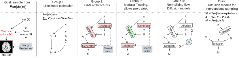
Figure 1: Suppose we aim to sample from $P(m|\text{do}(v))$, with $M$(MRI) as high-dimensional. Group 1 includes algorithms (ex: ID) that depend on likelihood estimation such as $P(m|v,a,b)$. Group 2 algorithms with GAN architectures have issues with GAN convergence while Group 3 improves convergence with modularization but both struggle to match the joint distribution. Group 4 utilizes normalizing flow, diffusion models, etc but cannot deal with confounders. Groups 2-4 only do unconditional interventions or costly rejection sampling. Finally, our method can employ classifier-free diffusion models to sample from $P(m|\text{do}(v))$ or conditional $P(m|a,do(v))$.

Although researchers have proposed deep neural networks for causal inference problems Shalit et al. (2017); Louizos et al. (2017) and neural causal methods Xia et al. (2021); Kocaoglu et al. (2018) to deal with high-dimensional data, the proposed approaches are not applicable to any general query due to restrictions they employ or their algorithmic design. For example, some approaches perform well only for low-dimensional discrete and continuous data (group 2 in Figure 1: (Xia et al., 2021; Balazadeh Meresht et al., 2022)) while some propose modular training to partially deal with high-dimensional variables (group 3: (Rahman & Kocaoglu, 2024)). Other works with better generative performance depend on a strong structural assumption: no latent variable in the causal graph (group 4: Kocaoglu et al. (2018); Pawlowski et al. (2020); Chao et al. (2023)).

Consider the graph in Figure 2. We are interested in observations of variable $Y$ after a hypothetical intervention on $X$, i.e, $Y\sim P(y|do(x)),\forall x$ (Pearl’s do-operator represents the intervention). The ID algorithm (Shpitser & Pearl, 2008) identifies this distribution in terms of the observational distribution by a complicated formula in Equation 1. If some variables are high-dimensional in this graph, explicit likelihood-based models cannot sample from the query, and previously mentioned methods can not generate good quality interventional samples since they might need to match the whole joint distribution $P(\mathbf{v})$ to learn the corresponding neural causal model.

$$\footnotesize\begin{split}&P(y|\text{do}(x))=\sum_{\mathbf{v}\setminus\{x,y\}}P_{\mathbf{v}\setminus\{w_{2},w_{3}\}}(w_{2},w_{3})P_{\mathbf{v}\setminus\{w_{4}\}}(w_{4})P_{\mathbf{v}\setminus\{w_{1}\}}(w_{1})P_{\mathbf{v}\setminus\{y\}}(y)\\ &=\sum_{w_{1},w_{2},w_{3},w_{4}}\frac{\sum_{x^{\prime}}P(w_{1},y|w_{2},w_{3},w_{4},x^{\prime})*P(x^{\prime}|w_{3},w_{4})}{\sum_{x^{\prime}}P(w_{1}|w_{2},w_{3},w_{4},x^{\prime})*P(x^{\prime}|w_{3},w_{4})}*P(w_{4}|w_{3})*P(w_{2}|w_{3},x)*P(w_{3})*\sum_{x^{\prime}}P(w_{1}|x^{\prime},w_{2},w_{3},w_{4})P(x^{\prime}|w_{3},w_{4})\end{split}$$ (1)

Figure 2: Double napkin graph and sampling network for $P_{x}(y)$.

In this paper, we show that it is possible to sample from any identifiable high-dimensional interventional distribution, in the presence of latent confounders, by leveraging deep conditional generative models. For example, we can design a network where each node consists of a set of conditional models as shown in Figure 2 to sample from the mentioned $P(y|\text{do}(x))$. This enables us to leverage state-of-the-art deep generative models, such as diffusion models. To train conditional models in our network for an arbitrary graph, our algorithm mimics the recursive trace of the Identification algorithm Shpitser & Pearl (2008). To the best of our knowledge, we are the first to show that conditional generative models are sufficient to sample from any identifiable causal effect estimand. Our contributions are as follows:

• We propose a recursive training algorithm called ID-DAG that learns a collection of conditional generative models using observational data and can sample from any identifiable interventional distribution.

• We show that ID-DAG is sound and complete, establishing that conditional generative models are sufficient to sample from any identifiable interventional query. Our guarantees extend to identifiable conditional interventional queries as well, which is especially challenging for existing GAN-based deep causal models.

• We use diffusion models to demonstrate ID-DAG’s performance on a colored-MNIST dataset. We also apply ID-DAG to quantify the role of spurious correlations in the generative models pre-trained on CelebA dataset.

2 Related Work

Over time, extensive literature has been developed on the causal effect estimation problem Bareinboim & Pearl (2012); Jaber et al. (2018); Lee et al. (2020). The use of deep neural networks for performing causal inference has been recently suggested by many researchers. Shalit et al. (2017); Louizos et al. (2017); Zhang et al. (2021); Vo et al. (2022) propose novel approaches to solve the causal effect estimation problem using variational autoencoders. However, their proposed solution and theoretical guarantees are tailored for specific causal graphs containing treatment, effect, and covariates (or observed proxy variables) where they can apply the backdoor adjustment formula. Sanchez & Tsaftaris (2022) employ energy-based generative models such as DDPMs (Ho et al., 2020) to generate high-dimensional interventional samples, but only for bivariate models. These works do not generalize to arbitrary structures.

Kocaoglu et al. (2018) train a collection of conditional generative models based on the causal graph and use adversarial training. Pawlowski et al. (2020) employed a conditional normalizing flow-based approach to offer high-dimensional interventional sampling as part of their solution. Chao et al. (2023) perform interventional sampling for arbitrary causal graphs employing diffusion-based causal models with classifier-free guidance (Ho & Salimans, 2022). Although these sampling-based approaches (Group 4 in Figure 1) can be used to generate high-quality interventional samples, their application is limited due to their strong assumption that the system has no unobserved confounders.

Xia et al. (2021) (Group 2 in Figure 1) propose similar architecture as Kocaoglu et al. (2018), adapting it to sample from interventional distributions in the presence of hidden confounders. However, their approach cannot handle high-dimensional variables, as they attempt to match the joint distribution involving such variables.  Rahman & Kocaoglu (2024)(Group 3) utilizes a modular fashion to relax the joint training restriction for specific structures. Nonetheless, their work might also face the convergence issue when the number of high-dimensional variables increases. Note that, these methods are not suitable for efficient conditional interventional sampling $P(y|z,\text{do}(x)),$ $\forall(x,z)$ as it is unclear how to update the posterior of $Z$’s upstream variables in their causal graph-based feedforward models.

Jung et al. (2020) convert the expression returned by  Tian & Pearl (2002) into a form where it can be computed through a re-weighting function, similar to propensity score-based methods, to allow sample-efficient estimation. However, computing these reweighting functions from data is still highly nontrivial with high-dimensional variables. Zečević et al. (2021) proposes an approach to model each probabilistic term in the expression obtained for $P(y|\text{do}(x))$ by using the do-calculus with (i)SPNs. However, their proposed method requires access to both observational and interventional data and does not address identification from only observations. Wang & Kwiatkowska (2023) design a novel probabilistic circuit architecture to encode the target causal query and estimate causal effects. They use do-calculus to obtain an expression and encode conditional/joint distributions of the expression in decomposable circuits. However, their method is not suitable for high-dimensional sampling.

3 Background

Definition 3.1 (Structural causal model, (SCM) (Pearl, 1980)).

An SCM is a tuple $\mathcal{M}=(G=(\mathcal{V},\mathcal{E}),\mathcal{N},\mathcal{U},\mathcal{F},P(.))$. $\mathcal{V}=\{V_{1},V_{2},...,V_{n}\}$ is a set of observed variables in the system. $\mathcal{N}$ is a set of independent exogenous random variables where $N_{i}\in\mathcal{N}$ affects $V_{i}$ and $\mathcal{U}$ is a set of unobserved confounders each affecting any two observed variables. This refers to the semi-Markovian causal model. A set of deterministic functions $\mathcal{F}$=$\{f_{V_{1}},f_{V_{2}},..,f_{V_{n}}\}$ determines the value of each variable $V_{i}$ from other observed and unobserved variables as $V_{i}=f_{i}(Pa_{i},N_{i},U_{S_{i}})$, where $Pa_{i}\subset\mathcal{V}$ (parents), $N_{i}\in\mathcal{N}$ (randomness) and $U_{S_{i}}\subset\mathcal{U}$ (common confounders) for some $S_{i}$. $\mathcal{P}(.)$ is a product probability distribution over $\mathcal{N}$ and $\mathcal{U}$ and projects a joint distribution $\mathcal{P}_{\mathcal{V}}$ over the set of actions $\mathcal{V}$ representing their likelihood.

An SCM $\mathcal{M}$, induces an acyclic directed mixed graph (ADMG) $G=(\mathcal{V},\mathcal{E})$ containing nodes for each variable $V_{i}\in\mathcal{V}$. For each $V_{i}=f_{i}(Pa_{i},N_{i},U_{S_{i}})$, $Pa_{i}\subset\mathcal{V}$, we add an edge $V_{j}\rightarrow V_{i}\in\mathcal{E},\forall V_{j}\in Pa_{i}$. Thus, $Pa_{i}(V_{i})$ becomes the parent nodes in $G$. $G$ has a bi-directed edge, $V_{i}\leftrightarrow V_{j}\in\mathcal{E}$ between $V_{i}$ and $V_{j}$ if and only if they share a latent confounder. If a path $V_{i}\rightarrow\ldots\rightarrow V_{j}$ exists, then $V_{i}$ is an ancestor of $V_{j}$, i.e., $V_{i}=An_{G}(V_{j})$. An intervention $\text{do}(x)$ replaces the structural function $f_{x}$ with $X=x$ and in other structural functions where $X$ occurs. The distribution induced on the observed variables $V$ after such an intervention is represented as $\mathcal{P}_{x}({v})$ or $\mathcal{P}({v}|\text{do}(x))$. Graphically, it is represented by $G_{\overline{X}}$ where incoming edges to $X$ are removed (we mark $X$ as red). With a slight abuse of notation, we will use $P(y)$ to represent both the numerical value $\mathbb{P}(Y=y)$ and the probability distribution $[P(y)]_{y}$, which will be clear from the context. Example usage for the latter will include “Let $Y$ be sampled from $P(y)$". Also, $P_{x}(y)$ refers to the interventional distribution for all $x,y$.

Definition 3.2 (c-component).

Given an ADMG $G$, a maximal subset of nodes where any two nodes are connected by bidirected paths is called a c-component $C(G)$.

Conditional Generative Models. The requirement for a conditional generative model is: given samples from a joint distribution, the model has to provide approximate samples from any conditional distribution. We use $M_{Y}(x)$ to refer to the model that can sample from $P(y|x)$, and illustrate it with a rectangle. The choice of generative models will depend on the application. For our purpose, we will use the classifier-free diffusion guidance (Ho & Salimans, 2021).

Identification algorithm:  Shpitser & Pearl (2008) propose the sound and complete ID algorithm for estimating an interventional distribution, $P_{x}(y)$ in semi-Markovian models. This algorithm applies the rules of do-calculus (Pearl, 1995) in a step-by-step recursive manner to convert $P_{x}(y)$ to some function of the observational distribution $\mathcal{P}_{\mathcal{V}}$.

4 Generative Models for Causal Sampling

Given a causal graph $G$, dataset $D\sim P(v)$, our objective is to generate samples from a causal query $P(y|\text{do}(x))$ or a conditional query $P(y|\text{do}(x),z)$. First, we express the challenges and outline our main ideas over a few examples.

4.1 Challenges and ID-DAG Motivation

Example 4.1.

To build intuition, we consider the graph in Figure 4(a). Consider the causal query $P_{x}(y)$. ID algorithm suggests $P_{x}(y)=$ $\sum_{z}P(z|w)P(y|x,w,z)$ which contains $W$ in the conditional distribution without any marginal. This raises the important question of where this $W$ comes from. Do-calculus ensures in this case that $P_{x}(y)=P_{x,w}(y)$; in other words, the causal effect of $W$ on $Y$ is irrelevant assuming we also intervene on $X$. Hence, we can pick any value of $W$ (ex: uniformly) to apply here. Now, suppose, we could sample from $P_{x,w}(y,z)$; in other words, suppose we had a mechanism that, when provided a value for $x,w$, would provide samples $(y,z)\!\sim\!P_{x,w}(y,z)$. From this, we can derive a way to sample from $P_{x,w}(y)$, by sampling $(y,z)\!\sim\!P_{x,w}(y,z)$ and only keeping the $y$ variable, i.e., dropping $Z$ from the joint sample is equivalent to sampling $Y$ from the distribution where $Z$ is marginalized out.

Now focusing on $P_{x,w}(y,z)$, ID gives $P_{x,w}(y,z)\!=\!P(y|x,w,z)P(z|w)$. From the joint dataset $\mathcal{D}$, we can train conditional generative models $M_{Z}$ and $M_{Y}$ to approximate sampling from these distributions. First, we attain a sampling mechanism $M_{Z}$ that samples $Z\sim P(z|w),\forall w$ and then attain a sampling mechanism $M_{Y}$ that provides sample access $P(y|x,w,z)$ (Figure 4(a)). We can arrange these mechanisms in a directed acyclic graph (DAG) called a sampling network, where sampling can be done according to the topological order, i.e, passing sampled values to descendant nodes. For any fixed intervention $X=x$, we perform interventional sampling, by picking any arbitrary values of $W$, using $M_{Z}(w)$ to get $Z$, and sampling $Y$ from $M_{Y}(x,w,z)$. Note that, for this specific example, we can also consider sampling according to the backdoor criterion but it would suggest sampling from $P(w,z)$ which requires unnecessarily training another mechanism $M_{W}$.

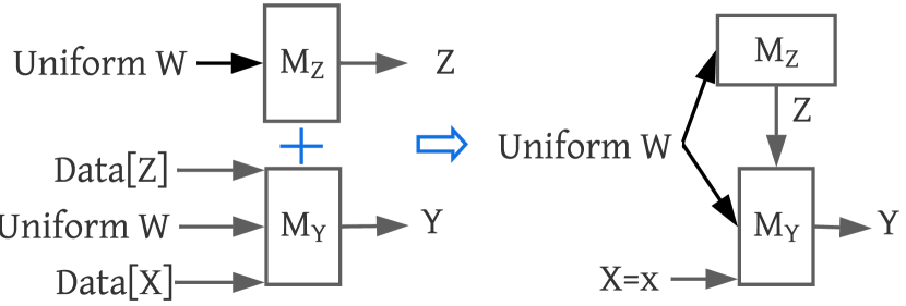
(a) Sampling from $P(y|\text{do}(x))=P(y|\text{do}(x,w))$ $=\sum_{z}P(z|w)$ $*P(y|x,w,z)$. $M_{Z}(w)$ and $M_{Y}(x,w,z)$ samples from $P(z|w)$ and $P(y|x,w,z)$. Merged network samples $P_{x}(y)$.

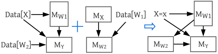
(b) Left network samples from $P_{x,w_{2}}(w_{1},y)$ $=P(w_{1}|x)$ $P(y|x,w_{1},w_{2})$. Right network samples from $P_{x,w_{1}}(w_{2})$ $=\sum_{x^{\prime}}P(x^{\prime})$ $P(w_{2}|x^{\prime},w_{1})$. Combinedly samples from $P_{x}(y)$.

Figure 4: High-dimensional interventional sampling of $P(y|\text{do}(x))$. Bi-directed edges indicate the presence of hidden confounders. Red nodes indicate the intervened variable.

Definition 4.2 (Sampling network, $\mathcal{H}$).

A collection of conditional generative models $\{M_{V_{i}}\}_{\forall_{i}}$ for a set of variables $\mathbf{V}=\{V_{i}\}_{\forall_{i}}$ is said to form a sampling network, $\mathcal{H}$, if the directed graph obtained by connecting each $M_{V_{i}}$ to $M_{An_{G}(V_{i})}$ via incoming edges is acyclic.

Note that our technical contribution should not be confused with standalone i)ancestral sampling or ii) conditional sampling at the ID algorithm base cases replacing the conditional distributions. Ancestral sampling following the topological order will not work in general for graphs with confounders. Direct conditional sampling in the ID algorithm might lead to a deadlock situation as shown in Example 4.3. Rather, ID-DAG utilizes these techniques as sub-procedures to sample from any interventional query in an ADMG.

Example 4.3 (cyclic dependency).

The graph in Figure 4(b) does not fit any familiar criterion such as backdoor or front door. The ID algorithm suggests that $P_{x}(y)=\sum_{w_{1},w_{2}}P_{x,w_{1}}(w_{2})\cdot P_{x,w_{2}}(w_{1},y)$ and estimates each of these factors sequentially. Suppose we naively follow the ID algorithm and attempt to sample from these factors sequentially as well. To sample $W_{2}\sim P_{x,w_{1}}(w_{2})$ we need $W_{1}$ as input, which has to be sampled from $P_{x,w_{2}}(w_{1},y)$. But to sample $\{W_{1},Y\}\sim P_{x,w_{2}}(w_{1},y)$, we need $W_{2}$ as input which has to be sampled from $P_{x,w_{1}}(w_{2})$. Therefore, no order helps to sample all $W_{1},W_{2},Y$ consistently.

Our algorithm, ID-DAG, solves this cyclic issue by avoiding direct sampling from the c-components. Rather, it first trains the required models for c-components $\{\{W_{2}\}$, $\{W_{1},Y\}\}$ individually, considering all possible input values. Next, it merges those models found in each c-component to build a single sampling network. We use this single sampling network to sample from $P_{x}(y),\forall x$. In Figure 4(b), we first obtain $P_{x,w_{2}}(w_{1},y)=P(w_{1}|x)P(y|x,w_{1},w_{2})$ and train a conditional model for each of the conditional distributions (left). Similarly, $P_{x,w_{1}}(w_{2})=\sum_{x^{\prime}}P(x^{\prime})P(w_{2}|x^{\prime},w_{1})$ and we train models for each distribution (right). We combine these two networks to construct the final network and perform ancestral sampling on it with the intervened values to obtain samples from $P_{x}(y)$.

4.2 ID-DAG: A Generative Model-based Algorithm for Interventional Sampling

Given a causal query $P_{\mathbf{x}}(\mathbf{y})$, a dataset $\mathcal{D}$ from the joint distribution $P$, and a causal graph $G$, ID-DAG builds a sampling network $\mathcal{H}$ where each node $M_{V_{i}}$ corresponds to a trained conditional generative model $M_{V_{i}}(.)$ that can generate samples from $P_{\mathbf{x}}(V_{i})$. Sampling from the interventional query $P_{\mathbf{x}}(\mathbf{y})$ can be performed by sampling each node in the topological order of $\mathcal{H}$. ID-DAG utilizes the recursive trace of the ID algorithm to obtain these trained conditional models from observational data and connect them together to build the sampling network $\mathcal{H}$.

Our key contribution is Algorithm 2: ID-DAG (see Appendix) which proceeds through a series of four recursive steps and reaches three possible base cases. For convenience, we provide the input/output in Algorithm 1 and describe the recursive steps and the base cases below. We also refer to Appendix E.1 for a simulation. Along with the given inputs $\mathbf{Y},\mathbf{X},G,\mathcal{D}$, ID-DAG maintains two additional parameters ${\hat{\mathbf{X}}}$: the set variables that are intervened at step 7s till the current recursion level; and ${\hat{{G}}}$: the same graph as $G$ except it contains ${\hat{\mathbf{X}}}$ with incoming edges deleted representing the intervention. We initiate with ID-DAG $(\mathbf{Y},\mathbf{X},G,\mathcal{D},{\hat{\mathbf{X}}}=\emptyset,{\hat{{G}}}=G)$.

Algorithm 1 ID-DAG$(\mathbf{Y},\mathbf{X},G,\mathcal{D},{{\hat{\mathbf{X}}}=\emptyset},{\hat{{G}}}=G)$

1:  Input: target $\mathbf{Y}$, to be intervened $\mathbf{X}$, intervened at step 7s ${\hat{\mathbf{X}}}$, causal graph $G$ without ${\hat{\mathbf{X}}}$, causal graph ${\hat{{G}}}$ with ${\hat{\mathbf{X}}}$ having no parents, training data $\mathcal{D}[{\hat{{G}}}]$.

2:  Output: A sampling network $\mathcal{H}$ of trained models.

3:  Recursive Steps 1-7.

Step 2: To enter step 2, ID-DAG checks if there exists any non-ancestor variable of $\mathbf{Y}$ (Step 2, line 1). Such variables in the graph do not have any causal effect on $\mathbf{Y}$. Thus, we safely drop them from all parameters. The next ID-DAG call with these updated parameters returns a network that can sample from the original query.

1:  if  ${\mathbf{V}}\setminus An({\mathbf{Y}})_{G}\neq\emptyset$  then {Step 2}

2:     Return ID-DAG($\mathbf{Y},\mathbf{X}\cap An(\mathbf{Y})_{G},$ $G_{An(\mathbf{Y})},$ $\mathcal{D}[An(\mathbf{Y})_{G}],$ ${{\hat{\mathbf{X}}}},$ ${\hat{{G}}}_{An(\mathbf{Y})}$ )

Step 3: ID-DAG checks if there exists a variable set $\mathbf{W}$ that can be included as additional intervention i.e., $\mathbf{X}=\mathbf{X}\cup\mathbf{W}$ without any effect on $\mathbf{Y}$ assuming that we already intervene on $\mathbf{X}$. Although $\mathbf{W}$ does not influence $\mathbf{Y}$, deleting (in future) the incoming edges to $\mathbf{W}$ will simplify the problem.

1:  Let $\mathbf{W}=(\mathbf{V}\setminus\mathbf{X})\setminus An(\mathbf{Y})_{G_{\overline{\mathbf{X}}}}$ {Step 3}

2:  if $\mathbf{W}\neq\emptyset$ then

3:     Return ID-DAG($\mathbf{Y},\mathbf{X}=\mathbf{X}\cup\mathbf{W},G,\mathcal{D},{{\hat{\mathbf{X}}}},{\hat{{G}}}$)

Step 4: If we remove $\mathbf{X}$ from $G$ and there exist multiple c-components in the remaining subgraph $G\setminus\mathbf{X}$ (Step 4:line 1) then we can apply c-component factorization (Lemma C.7, (Tian & Pearl, 2002)) to factorize $P_{\mathbf{x}}(\mathbf{y})$ as $P_{\mathbf{x}}(\mathbf{y})=\sum\limits_{\mathbf{v}\setminus(\mathbf{y}\cup\mathbf{x})}P_{\mathbf{v}\setminus s_{1}}(s_{1})P_{\mathbf{v}\setminus s_{2}}(s_{2})\ldots P_{\mathbf{v}\setminus s_{n}}(s_{n}).$ This implies that if we can obtain sampling networks $H_{i}$ for each $P_{\mathbf{v}\setminus s_{i}}(s_{i})$, we can wire them together based on their input-output to build one single sampling network $\mathcal{H}$, which will sample from $P_{\mathbf{x}}(\mathbf{y})$. To obtain such sampling networks, we perform the next recursive calls: ID-DAG$(\mathbf{Y}=S_{i},\mathbf{X}=\mathbf{V}\setminus S_{i},G,\mathcal{D},{{\hat{\mathbf{X}}}},{\hat{{G}}})$ for each of these c-components. Algorithm 4: ConstructDAG connects all returned $H_{i}$ to build the final $\mathcal{H}$.

1:  if $C(G\setminus\mathbf{X})=\{S_{1},\ldots,S_{k}\}$ then {Step 4}

2:     for each $S_{i}\in C(G\setminus\mathbf{X})=\{S_{1},\ldots,S_{k}\}$  do

3:        $\mathcal{H}_{i}=$ID-DAG$(S_{i},\mathbf{X}=\mathbf{V}\setminus S_{i},G,\mathcal{D},{{\hat{\mathbf{X}}}},{\hat{{G}}})$

4:     Return $\mathrm{ConstructDAG}(\{\mathcal{H}_{i}\}_{\forall i})$

Step 7: ID-DAG performs this step if i) $G\setminus\mathbf{X}$ is a single c-component $S$ and ii) $S$ is part of a larger c-component $S^{\prime}$ in the whole graph $G$, i.e, $(S=C(G\setminus\mathbf{X}))\subset(S^{\prime}\in C(G))$. For example, in Figure 14(b), for $P_{w_{1},w_{2},x}(y)$, we have $S=G\setminus\{W_{1},W_{2},X\}=\{Y\},S^{\prime}=\{W_{1},X,Y\}$. When ID-DAG visits step 7 for the first time, ${\hat{\mathbf{X}}}$ is an empty set. At this step, ID-DAG partitions the intervention set $\mathbf{X}$ into those that are contained within $S^{\prime}$, i.e., $\mathbf{X}\cap S^{\prime}$, and those that are not in $S^{\prime}$, i.e., $\mathbf{X}_{Z}=\mathbf{X}\setminus S^{\prime}$. ID algorithm asserts that evaluating $P_{\mathbf{x}}(\mathbf{y})$ from $P(\mathbf{v})$ is equivalent to evaluating $P_{\mathbf{x}\cap s^{\prime}}(\mathbf{y})$ considering $P_{\mathbf{x}_{z}}(\mathbf{v})$ as the joint distribution. Hence, we first perform $\text{do}(\mathbf{X}_{Z})$ on dataset $\mathcal{D}$ and then divert our goal of sampling from $P_{\mathbf{x}}(\mathbf{y})$ in $G$ with training dataset $\mathcal{D}\sim P(\mathbf{V})$ to sampling from $P_{\mathbf{x}\cap s^{\prime}}(\mathbf{y})$ in ${\hat{{G}}}_{\{S^{\prime},\overline{{\hat{\mathbf{X}}}}\}}$ with training data $\mathcal{D}\sim P_{\mathbf{x}_{z}}(\mathbf{v})$. We generate a dataset $\mathcal{D}\sim P_{\mathbf{x}_{z}}(\mathbf{v})$ with a sampling network $\mathcal{H}$ that we can obtain by a call to step 6 of ID-DAG (Step 7, line 2).

1:  if $C(G\setminus\mathbf{X})=\{S\}$ and ($\exists S^{\prime}$) such that $S\subset S^{\prime}\in C(G)$ then {Step 7}

2:     $\mathbf{X}_{Z}=\mathbf{X}\setminus S^{\prime}$,  $\mathcal{H}$ = RunStep6($S^{\prime},\mathbf{X}_{Z},G,\mathcal{D},{{\hat{\mathbf{X}}}},{\hat{{G}}}$),     $\mathcal{D}\sim\mathcal{H}(\mathbf{X}_{Z},{\hat{\mathbf{X}}})$

3:     ${{\hat{\mathbf{X}}}}={{\hat{\mathbf{X}}}}\cup\mathbf{X_{Z}}$

4:     Return ID-DAG($\mathbf{Y}$, $\mathbf{X}\cap S^{\prime}$, $G_{S^{\prime}}$, $\mathcal{D}[{{\hat{\mathbf{X}}}},S^{\prime}]$, ${{\hat{\mathbf{X}}}}$, ${\hat{{G}}}_{\{S^{\prime},\overline{{\hat{\mathbf{X}}}}\}}$)

Since the generated interventional dataset depends on the values of $\mathbf{X}_{Z}$, the models trained on this dataset in subsequent recursive steps will also depend on $\mathbf{X}_{Z}$. The values of $\mathbf{X}_{Z}$ might come from other c-components during ancestral sampling (ex: $M_{Y}(W_{2},*)$ in Figure 15), and we aim to make our trained models suitable for such inputs. Thus, during interventional data generation, unlike using a specific value in the ID algorithm, we pick values of $\mathbf{X}_{Z}$ from a uniform distribution or from $P(\mathbf{X}_{Z})$. We save $\mathbf{X}_{Z}$ in ${\hat{\mathbf{X}}}$, its values in $\mathcal{D}[{\hat{\mathbf{X}}},S^{\prime}]$ and in graph ${\hat{{G}}}$ with incoming edges removed. Since ${\hat{\mathbf{X}}}\neq\emptyset$ now, whenever ID-DAG visits step 7 again, ${\hat{\mathbf{X}}}$ will be applied along side new $\mathbf{X}_{Z}$. Finally, the recursive ID-DAG called at the current step with these updated parameters returns a network that samples from $P_{\mathbf{x}\cap S^{\prime}}(\mathbf{y})$ and equivalently from the original query $P_{\mathbf{x}}(\mathbf{y})$.

Base case, Step 5: Returns FAIL if $P_{x}(y)$ non-identifiable.

Base Cases: Step 1 & 6: ID-DAG enters step 1 if intervention $\mathbf{X}$ is empty. It enters step 6 if $\mathbf{Y}$ is contained in a single c-component $S\in C(G)$, and $\mathbf{X}$ is disjoint from $S$. When $\mathbf{X}=\emptyset$, $P_{\mathbf{x}}(\mathbf{y})=P(\mathbf{y})=\sum_{\mathbf{v}\setminus\mathbf{y}}P(\mathbf{v})=\sum_{\mathbf{v}\setminus\mathbf{y}}P(v_{i}|v_{\pi}^{(i-1)})$. For step 6, we can replace intervening on $\mathbf{X}$ by conditioning on $\mathbf{X}$, $P_{\mathbf{x}}(\mathbf{y})=\sum_{\mathbf{v}\setminus\mathbf{y}}P(v_{i}|v_{\pi}^{(i-1)})$. Therefore, both step 1 and 6, leverage samples from the dataset $\mathcal{D}$ to train a model $M_{V_{i}}$ for each variable $V_{i}$ in the c-component, using variables $V_{\pi}^{(i-1)}$ as inputs (Step 1/6, line 6). Note that ${\hat{\mathbf{X}}}$ is the set of variables that have been intervened on till now to update the training dataset $\mathcal{D}$ and ${\hat{{G}}}$ is the same graph as $G$ but contains ${\hat{\mathbf{X}}}$. Since we want the models $M_{V_{i}}$ to generate samples consistent with the values of ${\hat{\mathbf{X}}}$, $M_{V_{i}}$ is trained on $\mathcal{D}[{\hat{\mathbf{X}}},\mathbf{V}]$ and the input variables $V_{\pi}^{(i-1)}$ are ancestors of $V_{i}$ in ${\hat{{G}}}$ possibly containing some ${\hat{\mathbf{X}}}$. Finally, we build a sampling network by adding edges to $M_{V_{i}}$ from all its ancestor models in $\mathcal{H}$.

1:  if $\mathbf{X}=\emptyset$ or $(C(G\setminus\mathbf{X})=\{S\}$ and $S\in C(G))$ then {Step 1/ 6}

2:     $\mathcal{H}=\emptyset$

3:     for each $V_{i}\in\{\mathbf{X}\cup{{\hat{\mathbf{X}}}}\}$ do

4:        Add node $(M_{V_{i}}=\emptyset)$ to $\mathcal{H}$

5:     for each $V_{i}\in{S}$ in the topological order $\pi[{\hat{{G}}}]$ do

6:        Let $M_{V_{i}}$ be a model trained on $\{V_{i},V_{\pi}^{(i-1)}\}\sim\mathcal{D}$such that $M_{V_{i}}(V_{\pi}^{(i-1)})\sim P(v_{i}|v_{\pi}^{(i-1)})$

7:        Add node $(M_{V_{i}})$ to $\mathcal{H}$

8:        Add edge $M_{V_{j}}\rightarrow M_{V_{i}}$ to $\mathcal{H}$ for all $V_{j}\in V_{\pi}^{(i-1)}$

9:     Return $\mathcal{H}$.

Bottom up (Merging networks): During the top-down recursive steps, ID-DAG $i)$ makes the recursive calls based on the query, $ii)$ generates appropriate interventional datasets from the input observational samples to pass to the recursion, and $iii)$ trains conditional models to build sampling networks at base cases. During the bottom-up phase, ID-DAG returns a sampling network from each of its recursive steps. Finally, at step 4, ID-DAG receives multiple sampling networks, since it performed multiple recursive calls from this step. ID-DAG calls Algorithm 4:ConstructDAG (details in Appendix A.1) to merge all of them into a single sampling network $\mathcal{H}$ such that specific outputs of one c-component network are fed as input to other c-component networks.

Sampling: After the ID-DAG recursion ends, we specify intervened variables $\mathbf{X}=\mathbf{x}$ in the sampling network $\mathcal{H}$ and perform ancestral sampling according to $\mathcal{H}$’s topological order to generate joint samples. The $\mathbf{Y}$ values in these joint samples are the correct interventional samples of the original query $P_{\mathbf{x}}(\mathbf{y})$. Picking only values of $\mathbf{Y}$ is equivalent to marginalizing the rest. This step, performed at the end, plays the role of marginalization in the ID algorithm.

IDC-DAG: Conditional Interventional Sampling: Given a conditional causal query $P_{x}({y}|{z})$, we sample from this conditional interventional query by calling Algorithm 5: IDC-DAG. This function finds the maximal set ${\alpha}\subset{Z}$ such that we can apply do-calculus rule-2 and move ${\alpha}$ from conditioning set ${Z}$ and add it to intervention set ${X}$. Precisely, $P_{{x}}({y}|{z})=P_{{x\cup\alpha}}({y}|{z\setminus\alpha})=\frac{P_{{x\cup\alpha}}({y},{z\setminus\alpha})}{P_{{x\cup\alpha}}({z\setminus\alpha})}$. Next, Algorithm 2: ID-DAG(.) is called to obtain the sampling network that can sample from the interventional joint distribution $P_{{x\cup\alpha}}({y},{z\setminus\alpha})$. We use the sampling network to generate samples $\mathcal{D}[\mathbf{X}\cup\alpha,\mathbf{Y},\mathbf{Z}\setminus\alpha]$. We train a new conditional model $M_{{Y}}$ on $\mathcal{D}$ that takes ${Z\setminus\alpha}$, $X\cup\alpha$ as input and samples $Y\sim P_{{x\cup\alpha}}({y},{z\setminus\alpha})$ i.e, $Y\sim P_{x}(y|z)$.

Assumptions: i) the SCM is semi-Markovian, ii) we have access to the ADMG, iii) each trained conditional generative model correctly samples from the corresponding conditional distribution, and iv) $P(\mathbf{V})$ is strictly positive. We claim Thorem 4.4 and provide proofs in Appendix C &  D.

Theorem 4.4.

ID-DAG and IDC-DAG are sound and complete to sample from any identifiable $P_{x}(y)$ and $P_{x}(y|z)$.

5 Experiments

We evaluate ID-DAG on a semi-synthetic Colored MNIST and the real-world CelebA and Covid X-ray datasets. In the first experiment, we sample from $P_{x}(y)$ with $X$ and $Y$ both being images to illustrate ID-DAG’s ability to deal with high-dimensional variables. In the second experiment, ID-DAG estimates a causal query using large generative models as conditional models. These models are pre-trained on the CelebA dataset, and our goal is to evaluate the strength of spurious correlations and the level of disentanglement achieved by them. Finally, we also show our algorithm simulation on the Covid X-Ray dataset. We provide our code in https://github.com/Musfiqshohan/IDDAG and the training details in Appendix F.

5.1 Napkin-MNIST Dataset

Setup: We consider a semi-synthetic dataset corresponding to the napkin graph in Figure 6(b). We consider image variables $W_{1},X,Y$ that are derived from the Colored-MNIST dataset, and a paired discrete variable $W_{2}$. Image variables $X$ and $Y$ inherit the same digit value as image $W_{1}$ which is propagated through discrete $W_{2}.d\in[0-9]$. $X$ is either red or green which is also inherited from $W_{1}$ through discrete $W_{2}.c$, i.e., $W_{1}.color:\{r,g,b,y,m,c\}\rightarrow W_{2}.c:\{0,1\}\rightarrow X.color:\{r,g\}$. We introduce latent confounders $Ucolor$ and $Uthickness$. $Ucolor$ makes $W_{1}$ and $Y$ correlated with the same color while $Uthickness$ makes $W_{1}$ and $X$ correlated with the same thickness. We include a random noising process: with probability $0.1$ We provide the full data generation details in Appendix F.1. Our target is to sample from the distribution $P_{x}(y)$.

Component Models: Since $P_{x}(y)=P_{x,w_{1},w_{2}}(y)$, the sampling network for this query is built by step 1: generating an interventional dataset $P_{w_{2}}(x,y)$ and step 2: training a model $M_{Y}(x,w_{2})$ on this dataset. This trained model can sample from $P_{x}(y)$. Step 1: Given samples $\mathcal{D}\!\sim\!P(v)$, we need to first generate an interventional dataset $\mathcal{D}^{\prime}$ for $W_{2},X,Y$ from $P_{w_{2}}(x,y)$, or equivalently just the $W_{2},X,Y$ samples from $P(w_{1})P(x,y|w_{1},w_{2})$. Sampling from $P(x,y|w_{1},w_{2})$ can be done by learning a conditional diffusion model trained on the observational distribution $P(v)$. Thus we obtain $\mathcal{D}^{\prime}$, by sampling $W_{1}\!\sim\!P(w_{1})$, choosing an arbitrary $W_{2}$, and sampling from the trained diffusion model. Step 2: We learn a diffusion model $M_{Y}(x,w_{2})$ to sample from $P(y|x,w_{2})$ by training on the new dataset $\mathcal{D}^{\prime}$.
Baselines: We compared our algorithm with two baselines: Baseline 1: A classifier-free diffusion model that samples from the conditional distribution: $Y\sim P(y|x)$. Baseline 2: The NCM algorithm (Xia et al., 2021) that samples from the interventional distribution $P_{x}(y)$.

Evaluation: Although we do not have access to true interventional images, we evaluate our approach in two parts.
i) Correctness w.r.t ground truth (Figure 6(a)): We present generated samples from the trained diffusion models. If we can map our generated images to discrete analogues $(Digit,Color,Thickness)$ and compute exact likelihoods, we can compare them with our ground truth to evaluate the correctness of these samples. Thus, we utilize trained classifiers to identify discrete properties such digit, color, and thickness of the $P_{x}(y)$ sampled images and compare them to the true (discrete) interventional and conditional distributions. We display these results for the color attribute in Figure 6(a) and see that our sampling much more closely emulates the interventional distribution (almost uniform) than the true conditional (imbalanced).

ii) Comparison w.r.t baselines: We choose two images i) of digit 3 and ii) of digit 5, both colored red as the intervention value for $X$. Then we used these images to sample from $P(y|x)$ and $P_{x}(y)$ distributions using ID-DAG and the baselines (Figure 6(b)). The conditional model (row 1, row 4) and our algorithm (row 2, row 5) both generate high-quality images of digit 3 and digit 5 with a specific color from the six possible colors. Whereas, the colors in generated images from the NCM algorithm (row 3, row 6) can not remain at any specific value and get blended (such as green+yellow, etc). We also provide the Frechet Inception Distance (FID) of each method (the lower the better). The score for good-quality images changes for different datasets. Here, we considered the score with respect to our ground truth image dataset. We observe that our algorithm has the lowest FID score, i.e., our algorithm generates the most high-quality images from interventional distribution. Also, since ID-DAG removes the backdoor path of $X$ and $Y$, it shows all colors with almost uniform probability unlike the conditional which shows bias towards R, G and B. This is consistent with the observation in Figure 6(a).

	Red	Green	Blue	Yellow	Magenta	Cyan
$\mathbf{\hat{P}(y.c\mid Do(x.c=R))}$	0.160	0.181	0.164	0.177	0.170	0.147
$P(y.c\mid Do(x.c=R))$	0.167	0.167	0.167	0.167	0.167	0.167
$P(y.c\mid x.c=R)$	0.276	0.276	0.276	0.057	0.057	0.057
$\mathbf{\hat{P}(y.c\mid Do(x.c=G))}$	0.159	0.176	0.163	0.178	0.173	0.150
$P(y.c\mid Do(x.c=G))$	0.167	0.167	0.167	0.167	0.167	0.167
$P(y.c\mid x.c=G)$	0.057	0.057	0.057	0.276	0.276	0.276

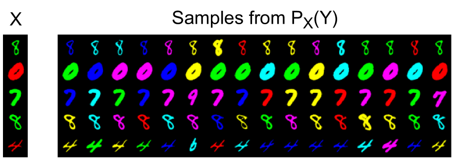
(a) (Left): Color distributions of generated samples of $P_{x}(y)$, where $V.c$ refers to the image color. ID-DAG samples are fed into a color classifier and $\hat{P}$ is the distribution over its output. All other values are the ground truth on the discrete Napkin-MINST. Our samples’ colors closely reflect the true interventions than other candidate distributions. (Right): Samples from the interventional distribution $P_{x}(y)$.

	Baseline -1 Conditional Model	Baseline -2 NCM	Ours ID-DAG
FID score	67.012	71.646	43.507

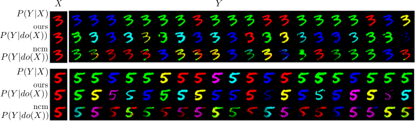
(b) (Left): The causal graph for the Napkin-MNIST dataset and the FID scores (lower the better). Scores of baseline 1, baseline 2 and our algorithm are calculated with respect to the training images. (Right): Baseline 1, $P(y|x)$: row 1,4 shows bias towards [R, G, B]. Ours $P(y|\text{do}(x))$: row 2,5 shows all colors. NCM $P(y|\text{do}(x))$: row 3,6 shows incorrect blended colors.

Figure 6: Semi-synthetic Napkin MNIST experiment.

5.2 CelebA: Image to Image Translation

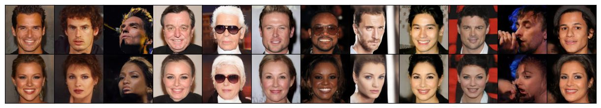
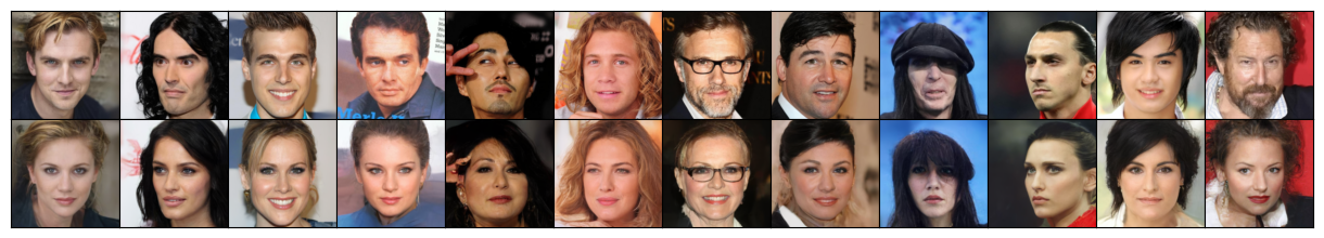
Figure 17: Multi-domain image translation by EGSDE. Images in rows 1 and 3 are the original images (male domain) and images in rows 2 and 4 are translated images (female domain). Table 4 shows, 29.16% of the total images are translated as a young person.

Setup: In this experiment, we explain the multi-domain image-to-image translation of generative models. We examine if the image translation is causal or if any unnecessary features are being added due to the spurious correlations in their training data. Our application is motivated by Goyal et al. (2019), who generate counterfactual images to explain a pre-trained classifier while we examine pre-trained image generative models. More precisely, we evaluate which facial attributes a model affects while translating an image from the $\mathrm{Male}$ domain to the $\mathrm{Female}$ domain. Spurious changes might be hard for human eyes to detect (for example the $\mathrm{Female}$-$\mathrm{Young}$ correlation in the 24 images in Figure 17). Our goal is to assess spurious correlations large generative models learn among different attributes from their training data. For this purpose, we employ two generative models that are trained on the CelebA dataset (Liu et al., 2015), i) StarGAN (Choi et al., 2018): a generative adversarial network and ii) EGSDE (Zhao et al., 2022): an approach that utilizes energy-guided stochastic differential equations, to translate images from the $\mathrm{Male}$ domain to the $\mathrm{Female}$ domain. After translation, we observe what causal and non-causal attributes the model has changed.

We assume the graph in Figure 7(a) where the original image $I_{1}$ causes its own attributes $\mathrm{Male}$ and $\mathrm{Young}$. These attributes along with the original image are used to generate a translated image $I_{2}$. We use a classifier to predict all 40 attributes of $I_{1}$ as $P_{1}$ and of $I_{2}$ as $P_{2}$. Variable $A$ represents the additional attributes (ex: Makeup) that are being added to $I_{2}$ but absent in $I_{1}$ during the translation. Our target is to estimate $P(A|\text{do}(\mathrm{Male}=0))$, i.e., what is the causal effect of changing the $\mathrm{Male}$ domain to the $\mathrm{Female}$ domain on the appearance of a new attribute? We can shift the target to $P(I_{2}|\text{do}(\mathrm{Male}=0))$ and then use the classifier on $I_{2}$.

After running ID-DAG on the query, we obtain the sampling network in Figure 7(a). ID-DAG instructs to first sample $I_{1}\sim M_{I_{1}}$ and $\mathrm{Young}\sim M_{Y}$ and then feed $\mathrm{Male}=0,\mathrm{Young},I_{2}$ into a generative model $M_{I_{2}}(.)$ to generate samples of $I_{2}$. Now, instead of training $M_{I_{2}}$, we can plug in the model that we want to evaluate (StarGAN or EGSDE) and since we have the dataset samples of $I_{1},\mathrm{Young}$, we can directly feed those in $M_{I_{2}}(.)$ for this specific graph. Thus, we sample around 850 samples of $\mathrm{Young},I_{1}$ from the CelebA dataset, i.e, images of different ages, and feed them into our selected pre-trained generative model. Note that this sampling mechanism is consistent with the ID algorithm derivation: $P(I_{2}|\text{do}(\mathrm{Male}=0))=\int_{\mathrm{Young},I_{1}}P(I_{2}|\mathrm{Male}=0,\mathrm{Young},I_{1})P(\mathrm{Young},I_{1})$ Next, we used a pre-trained classifier to obtain 40 attributes of $I_{1}$ and $I_{2}$ as $P_{1}$ and $P_{2}$. Finally, we obtain the additional added attributes, $A$ by comparing $P_{1}$ and $P_{2}$ for each of 850 samples and the proportion is reported as the estimate of $P(A|\text{do}(\mathrm{Male}=0))$. We perform the above ID-DAG process for both StarGAN and EGSDE independently. We do the same but fix $\mathrm{Young}=1$ for estimating the conditional causal effect, $P(A|\mathrm{Young},\text{do}(\mathrm{Male}=0))$ with a Conditional StarGAN.

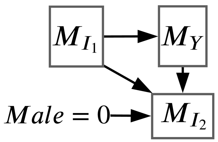
(a) Causal graph for image to image translation.

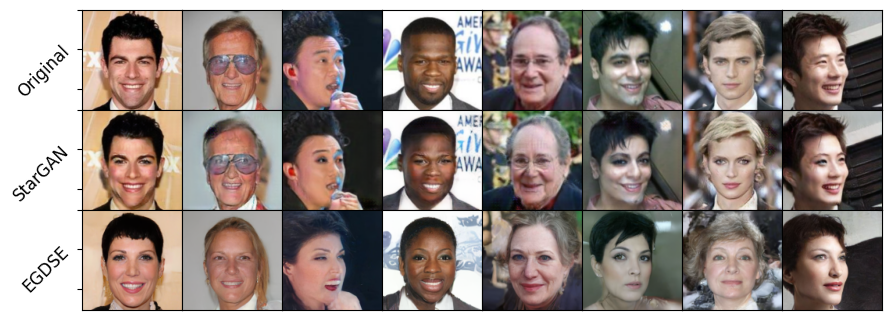
(b) Samples from $P(I_{2}|do(Male=0)$. Row 1: original $I_{1}$, Row 2: translated $I_{2}$ by StarGAN and Row3: translated $I_{2}$ by EGSDE.

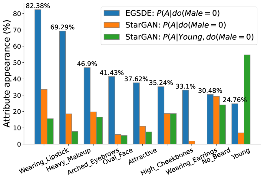
(c) Unconditional/conditional causal effect on the appearance of specific attributes.

Figure 7: Male domain to female domain translation. EGSDE generates images with different causal attributes such as $\mathrm{WearingLipstick}$, $\mathrm{HeavyMakeup}$ and $\mathrm{WearingEarrings}$ but also adds non-causal attributes such as $\mathrm{Attractive}$ and $\mathrm{Young}$ due to the correlation with $\mathrm{Female}$ in the training data. StarGAN shows a low correlation with both causal and non-causal images which is also not preferred.

Evaluation: We show results for the top 11 attributes that appeared most, in Figure 7(c). We observed that EGSDE introduces new attributes more compared to StarGAN. For example, during $\mathrm{Male}$ to $\mathrm{Female}$ image translation, EGSDE adds $\mathrm{WearingLipstick}$ attribute to $82\%$ of all images. It also introduces other causally related attributes such as $\mathrm{HeavyMakeup}(69.28\%),\mathrm{WearingEarrings}(33.09\%)$, $\mathrm{NoBeard}(30.47\%)$, etc with high probability. EGSDE also introduces $\mathrm{Attractive}(37.61\%)$ and $\mathrm{Young}(24.76\%)$ which should not be causally related to a $\mathrm{Female}$ attribute. We interpret the reason behind these appearances as that they are spuriously correlated in the CelebA training dataset. For example, sex and age have a correlation coefficient of 0.42  (Shen et al., 2020). On the other hand, StarGAN and conditional StarGAN introduce any new attribute with a low probability ($\leq 30\%)$ even for the causally related attributes which is not preferred. However, conditional StarGAN translates $54.68\%$ of images as $\mathrm{Female},\mathrm{Young}$ which is consistent with its causal query $P(A|\mathrm{Young},\text{do}(\mathrm{Male}=0))$. Therefore, these evaluations have implications on fairness and ID-DAG can play an important role estimating them.

Baselines: Existing algorithms such as  Xia et al. (2023); Chao et al. (2023) do not utilize the causal effect expression of $P(A|do(\mathrm{Male}=0))$, rather they train neural models for each variable in the causal graphs which will be costly in this scenario. Even if they utilize pre-trained models, they have to train models for the remaining variables to match the whole joint and perform sampling-based methods to evaluate $P(A|\mathrm{Young}=1,do(\mathrm{Male}=0))$.

5.3 Covid X-Ray Dataset

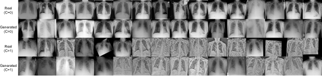
Figure 8: Generated Covid XRay Images: Generated chest XRay images from our diffusion model, separated by class and compared against real data.

Table 1: (Left) Class-conditional FID scores for generated Covid XRAY images (lower is better). Generated $C=c$, means we sample from the diffusion model conditioned on $c$. Real $(C=c)$ refers to a held out test set of approximately 5k images, partitioned based on $C$-value. Low values on the diagonal and high values on the off-diagonal imply we are sampling correctly from conditional distributions. (Right) Evalution of Interventional Distribution $P_{c}(n)$. We evaluate the distributions $P_{c}(n=1)$ for three cases for the Covid-XRAY dataset. Diffusion uses a learned diffusion model for $P(x|c)$, No Diffusion samples $P(x|c)$ empirically from a held out validation set, and no latent evaluates the conditional query assuming no latent confounders in the causal model.

FID $(\downarrow)$	Real: $C=0$	Real: $C=1$
Generated: $C=0$	15.77	61.29
Generated $C=1$	101.76	23.34

$P_{c}(n=1)$	$c=0$	$c=1$
Diffusion	0.622	0.834
No Diffusion	0.623	0.860
No Latent	0.406	0.951

Data generation: Next we apply our algorithm to a real dataset using chest X-rays on COVID-19 patients. Specifically, we download a collection of chest X-rays (X) where each image has binary labels for the presence/absence of COVID-19 (C), and pneumonia (N) (Wang et al., 2020) . We imbue the causal structure of the backdoor graph, where $C\to X$, $X\to N$, and there is a latent confounder affecting both $C$ and $N$ but not $X$. This may capture patient location, which might affect the chance of getting COVID-19, and quality of healthcare affecting the right diagnosis. Since medical devices are standardized, location would not affect the X-ray image given COVID-19. We are interested in the interventional query $P_{c}(n)$: the treatment effect of COVID-19 on the presence of pneumonia.

Component Models: Applying ID-DAG to this graph requires access to two conditional distributions: $P(x|c)$ and $P(n|x,c)$. Since $X$ is a high-dimensional image, we train a conditional diffusion model to approximate the former. Since $N$ is a binary variable, we train a classifier that accepts $X,C$ and returns a Bernoulli distribution for $N$. The generated sampling network operates by sampling an $X$ given the interventional $C$, and then sampling an auxiliary $C^{\prime}\sim P(c^{\prime})$ and feeding $X,C^{\prime}$ to the classifier for $P(n|x,c)$, finally sampling from this distribution.

Evaluation: Again we do not have access to the ground truth. Instead, we focus on the evaluation of each component model, and we also perform an ablation on our diffusion model. We first evaluate the image quality of the diffusion model approximating $P(x|c)$. We evaluate the FID of generated samples versus a held-out validation set of 10K X-ray images. When samples are generated with $C$ taken from the training distribution, we attain an FID score of $16.17$. We then evaluate the conditional generation by comparing class-separated FID evaluations and display these results in Table 1 (left). The classifier estimating $P(n|x,c)$ has an accuracy of 91.9% over validation set. We note that we apply temperature scaling (Guo et al., 2017) to calibrate our classifier, where the temperature parameter is trained over a random half of the validation set. Temperature scaling does not change the accuracy, but it does vastly improve the reliability metrics; see Appendix.

Finally we evaluate the query of interest $P_{c}(n)$. Since we cannot evaluate the ground truth, we consider our evaluated $P_{c}(n)$ versus an ablated version where we replace the diffusion sampling mechanism with $\hat{P}(x|c)$, where we randomly select an X-ray image from the held-out validation set. We also consider the query $P_{c}(n)$ if there were no latent confounders in the graph, in which case, the interventional query $P_{c}(n)$ is equal to $P(n|c)$. We display the results in Table 1 (right).

6 Conclusion

We propose a sound and complete algorithm to sample from conditional or unconditional high-dimensional interventional distributions. Our approach is able to leverage the state-of-the-art conditional generative models by showing that any identifiable causal effect estimand can be sampled from, only via forward generative models. In future works, we aim to relax our assumption on access to the ADMG.

Appendix A Appendix: Pseudo-codes

Algorithm 2 ID-DAG$(\mathbf{Y},\mathbf{X},G,\mathcal{D},{{\hat{\mathbf{X}}}=\emptyset},{\hat{{G}}}=G)$

1:  Input: target $\mathbf{Y}$, to be intervened $\mathbf{X}$, intervened variables at step 7s ${\hat{\mathbf{X}}}$, causal graph $G$ without ${\hat{\mathbf{X}}}$, causal graph ${\hat{{G}}}$ with ${\hat{\mathbf{X}}}$ having no parents, training data $\mathcal{D}[{\hat{{G}}}]$ sampled from the distribution Markov relative to ${\hat{{G}}}$.

2:  Output: A DAG of trained models.

3:  if $\mathbf{X}=\emptyset$ then {Step 1}

4:    $\mathcal{H}=\emptyset$

5:    for each $V_{i}\in{{\hat{\mathbf{X}}}}$ do

6:      Add node $(V_{i},\emptyset)$ to $\mathcal{H}$

7:    for each $V_{i}\in\mathbf{Y}$ in the topological order $\pi[{\hat{{G}}}]$ do

8:      Let $M_{V_{i}}$ be a model trained on $\{V_{i},V_{\pi}^{(i-1)}\}\sim\mathcal{D}$ such that $M_{V_{i}}(v_{\pi}^{(i-1)})\sim P(v_{i}|v_{\pi}^{(i-1)})$

9:      Add node $(V_{i},M_{V_{i}})$ to $\mathcal{H}$

10:      Add edge $V_{j}\rightarrow V_{i}$ to $\mathcal{H}$ for all $V_{j}\in\{V_{\pi}^{(i-1)}\}$

11:    Return $\mathcal{H}$

12:  if  $\mathbf{V}\setminus An(\mathbf{Y})_{G}\neq\emptyset$  then {Step 2}

13:    Return ID-DAG($\mathbf{Y},\mathbf{X}\cap An(\mathbf{Y})_{G},$ $G_{An(\mathbf{Y})},$ ${{\hat{\mathbf{X}}}},$ ${\hat{{G}}}_{An(\mathbf{Y})},$ $\mathcal{D}^{\prime}=\mathcal{D}[An(\mathbf{Y})_{G}]$ )

14:  Let $\mathbf{W}=(\mathbf{V}\setminus\mathbf{X})\setminus An(\mathbf{Y})_{G_{\overline{\mathbf{X}}}}$ {Step 3}

15:  if $\mathbf{W}\neq\emptyset$ then

16:    Return ID-DAG($\mathbf{Y},\mathbf{X}=\mathbf{X}\cup\mathbf{W},G,{{\hat{\mathbf{X}}}},{\hat{{G}}},\mathcal{D}$)

17:  if $C(G\setminus\mathbf{X})=\{S_{1},\ldots,S_{k}\}$ then {Step 4}

18:    for each $S_{i}\in C(G\setminus\mathbf{X})=\{S_{1},\ldots,S_{k}\}$  do

19:      $\mathcal{H}_{i}$=ID-DAG$(S_{i},\mathbf{X}=\mathbf{V}\setminus S_{i},G,{{\hat{\mathbf{X}}}},{\hat{{G}}},\mathcal{D})$

20:    Return $\mathrm{ConstructDAG}(\{\mathcal{H}_{i}\}_{\forall i})$

21:  if $C(G\setminus X)=\{S\}$ then

22:    if $C(G)=\{G\}$  then {Step 5}

23:      throw FAIL

24:    if $S\in C(G)$ then {Step 6}

25:      $\mathcal{H}=\emptyset$

26:      for each $V_{i}\in\{\mathbf{X}\cup{{\hat{\mathbf{X}}}}\}$ do

27:         Add node $(V_{i},\emptyset)$ to $\mathcal{H}$

28:      for each $V_{i}\in{S}$ in the topological order $\pi[{\hat{{G}}}]$ do

29:         Let $M_{V_{i}}$ be a model trained on $\{V_{i},V_{\pi}^{(i-1)}\}\sim\mathcal{D}$ such that $M_{V_{i}}(V_{\pi}^{(i-1)})\sim P(v_{i}|v_{\pi}^{(i-1)})$

30:         Add node $(V_{i},M_{V_{i}})$ to $\mathcal{H}$

31:         Add edge $V_{j}\rightarrow V_{i}$ to $\mathcal{H}$ for all $V_{j}\in V_{\pi}^{(i-1)}$

32:      Return $\mathcal{H}$.

33:    if ($\exists S^{\prime}$) such that $S\subset S^{\prime}\in C(G)$ then {Step 7}

34:      $\mathbf{X}_{Z}=\mathbf{X}\setminus S^{\prime}$,    $\mathcal{H}$ = RunStep6($S^{\prime},\mathbf{X}_{Z},G,\mathcal{D},{{\hat{\mathbf{X}}}},{\hat{{G}}}$),     $\mathcal{D}\sim\mathcal{H}(\mathbf{X}_{Z},{\hat{\mathbf{X}}})$

35:      ${{\hat{\mathbf{X}}}}={{\hat{\mathbf{X}}}}\cup\mathbf{X_{Z}}$

36:      Return ID-DAG($\mathbf{Y}$, $\mathbf{X}\cap S^{\prime}$, $G_{S^{\prime}}$, $\mathcal{D}[{{\hat{\mathbf{X}}}},S^{\prime}]$, ${{\hat{\mathbf{X}}}}$, ${\hat{{G}}}_{\{S^{\prime},\overline{{\hat{\mathbf{X}}}}\}}$)

Algorithm 3 RunStep6($\mathbf{Y},\mathbf{X},G,\mathcal{D},{{\hat{\mathbf{X}}}},{\hat{{G}}}$)

1:  Input: target $\mathbf{Y}$, to be intervened $\mathbf{X}$ , intervened at step 7s ${\hat{\mathbf{X}}}$ of $\mathbf{Y}$, causal graph $G$ without ${\hat{\mathbf{X}}}$, causal graph ${\hat{{G}}}$ with ${\hat{\mathbf{X}}}$ having no parents, training data $\mathcal{D}[{\hat{{G}}}]$ sampled from the distribution Markov relative to ${\hat{{G}}}$.

2:  Output: A DAG of trained models.

3:  $\mathcal{H}=\emptyset$

4:  for each $V_{i}\in\{\mathbf{X}\cup{{\hat{\mathbf{X}}}}\}$ do

5:    Add node $(V_{i},\emptyset)$ to $\mathcal{H}$

6:  for each $V_{i}\in{S}$ in the topological order $\pi[{\hat{{G}}}]$ do

7:    Let $M_{V_{i}}$ be a model trained on $\{V_{i},V_{\pi}^{(i-1)}\}\sim\mathcal{D}$ such that $M_{V_{i}}(V_{\pi}^{(i-1)})\sim P(v_{i}|v_{\pi}^{(i-1)})$

8:    Add node $(V_{i},M_{V_{i}})$ to $\mathcal{H}$

9:    Add edge $V_{j}\rightarrow V_{i}$ to $\mathcal{H}$ for all $V_{j}\in V_{\pi}^{(i-1)}$

10:  Return $\mathcal{H}$.

Algorithm 4 ConstructDAG($\{H_{i}\}_{\forall i}$)

1:  Input: A set of disconnected DAG sampling networks, each containing trained models: $\{H_{i}\}_{\forall i}$.

2:  Output: A connected DAG sampling network $\mathcal{H}$.

3:  for  $H_{i}\in\{H_{i}\}_{\forall i}$ do

4:    for $M_{V_{j}}\in H_{i}$ do

5:      if $M_{V_{j}}=\emptyset$ and $\exists M_{V_{k}}\in H_{r},\forall r$ such that $V_{j}=V_{k}$ and $M_{V_{k}}\neq\emptyset$ then {Searches for a trained model to generate $V_{j}$}

6:         $M_{V_{j}}=M_{V_{k}}$

7:  $\mathcal{H}$= $\{H_{i}\}_{\forall i}$ {All $H_{i}$ are connected now.}

8:  Return $\mathcal{H}$

Algorithm 5 IDC-DAG($\mathbf{Y},\mathbf{X},\mathbf{Z},\mathcal{D},G$)

1:  Input: target ${Y}$, intervention ${X}$ , conditioning set ${Z}$. training data $\mathcal{D}$, $G$.

2:  Output: A DAG of trained model to sample from $P_{\mathbf{X}}(\mathbf{Y|Z})$.

3:  if  $\exists\alpha\in Z$ such that $({Y}\perp\!\!\!\perp\alpha|{X},{Z}\setminus\{\alpha\})_{G_{\overline{{X}},\underline{\alpha}}}$ then

4:    return IDC-DAG(${Y},{X}\cup\{\alpha\},{Z}\setminus\{\alpha\},\mathcal{D},G$)

5:  else

6:    $H_{1}$= ID-DAG(${Y\cup Z},{X},\mathcal{D},{\hat{\mathbf{X}}}=\emptyset,{\hat{{G}}}=G$)

7:    $\mathcal{D}^{\prime}\sim H_{1}({X})$

8:    $H_{2}=\emptyset$

9:    Add node $(X,\emptyset)$ and $(Z,\emptyset)$ to $H_{2}$

10:    Let $M_{Y}$ be a model trained on $\{Y,X,Z\}\sim\mathcal{D}^{\prime}$ such that $M_{Y}(X,Z)\sim P^{\prime}(Y|X,Z)$ i.e., $M_{Y}(X,Z)\sim P_{X}(Y|Z)$

11:    Add node $(Y,M_{Y})$ to $H_{2}$

12:    Add edge $X\rightarrow Y$ and $Z\rightarrow Y$ to $H_{2}$

13:    return $H_{2}$

Algorithm 6 ID($\mathbf{y},\mathbf{x},P,G$)

1:  Input: $\mathbf{y}$, $\mathbf{x}$ value assignments , distribution $P$, $G$.

2:  Output: Expression for $P_{\mathbf{x}}(\mathbf{y})$ in terms of $P$ or Fail$(F,F^{\prime})$.

3:  if $\mathbf{x}=\emptyset$  then {Step:1}

4:    Return $\sum_{\mathbf{v}\setminus\mathbf{y}}P(\mathbf{v})$

5:  if $\mathbf{V}\setminus An(\mathbf{Y})_{G}\neq\emptyset$ then {Step:2}

6:    Return ID($\mathbf{y},\mathbf{x}\cap An(\mathbf{Y})_{G},\sum_{\mathbf{V}\setminus An(\mathbf{Y})_{G}}P,G_{An(\mathbf{Y})}$)

7:  Let $\mathbf{W}=(\mathbf{V}\setminus\mathbf{X})\setminus An(\mathbf{Y})_{G_{\overline{\mathbf{X}}}}$ {Step:3}

8:  if $\mathbf{W}\neq\emptyset$ then

9:    Return ID$(\mathbf{y},\mathbf{x}\cup\mathbf{w},P,G)$

10:  if $C(G\setminus\mathbf{X})=\{S_{1},\ldots,S_{k}\}$ then {Step:4}

11:    Return $\sum_{\mathbf{v\setminus(y\cup x)}}\prod_{i}ID(s_{i},\mathbf{v}\setminus s_{i},P,G)$

12:  if $C(G\setminus\mathbf{X})=\{S\}$ then

13:    if $C(G)=\{G\}$ then {Step:5}

14:      Return FAIL$(G,G\cap S)$

15:    if $S\in C(G)$ then {Step:6}

16:      Return $\sum_{s\setminus\mathbf{y}}\prod_{\{i|V_{i}\in S\}}P(v_{i}|v_{\pi}^{i-1})$

17:    if $\exists S^{\prime}$ s.t. $S\subset S^{\prime}\in C(G)$ then {Step:7}

18:      Return ID$(\mathbf{y},\mathbf{x}\cap S^{\prime},{P}=\prod_{\{i|V_{i}\in S^{\prime}\}}P(V_{i}|V_{\pi}^{(i-1)}\cap S^{\prime},v_{\pi}^{(i-1)}\setminus S^{\prime}),G_{S^{\prime}})$

Algorithm 7 IDC(${Y},{X},{Z},P,G$)

1:  Input: $x,y,z$ value assignments, $P$ a probability distribution, $G$ a causal diagram (an I-map of $P$).

2:  Output: Expression for $P_{{X}}({Y|Z})$ in terms of $P$ or Fail(F,F’).

3:  if  $\exists\alpha\in Z$ such that $({Y}\perp\!\!\!\perp\alpha|{X},{Z}\setminus\{\alpha\})_{G_{\overline{{X}},\underline{\alpha}}}$ then

4:    return IDC(${Y},{X}\cup\{\alpha\},{Z}\setminus\{\alpha\},\mathcal{D},G$)

5:  else

6:    let $P^{\prime}$ = ID($\mathbf{y\cup z,x},P,G$)

7:    return $P^{\prime}/\sum_{\mathbf{y}}P^{\prime}$

A.1 Sub-Procedure: ConstructDAG

In Algorithm 4: , each sampling network $H_{i}$ is a set of conditional trained models connected with each other according to a directed acyclic graph. Any node in the sampling network represents a trained generative model $M_{V_{j}}$ for variable $V_{j}$. This sub-procedure takes multiple sampling networks $\{H_{i}\}_{\forall_{i}}$ as input and combines them to construct a larger consistent sampling network $\mathcal{H}$. We iterate over each nodes $M_{V_{j}}$ in each sampling network $H_{i}$ (lines 3-4). If $M_{V_{j}}=\emptyset$, i.e., it does not contain any trained model, then either $V_{j}$ is intervened on and it does not need a model or it must have its trained model located in some other sampling network $H_{r}$ as node $M_{V_{k}}$. When we find that node $M_{V_{k}}$ in some other sampling network $H_{r}$ by checking $V_{j}=V_{k}$ (line 5), we connect $H_{i}$ and $H_{r}$ by combining $M_{V_{j}}$ and $M_{V_{k}}$ (line 6) since $V_{j}$ and $V_{k}$ are the same variable. In this manner, we combine all sampling networks to construct one single network $\mathcal{H}$ (line 7).

Appendix B Causal query expressions

B.1 Double Napkin mentioned in Section 1

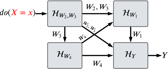
Figure 9: Double napkin graph and sampling network for $P_{x}(y)$.

For $P_{x}(y)$ in Figure 2 or Figure 9 we have:

$$\footnotesize\begin{split}&P(y|\text{do}(x))\\ &=\sum_{\mathbf{v}\setminus\{x,y\}}P_{\mathbf{v}\setminus\{w_{2},w_{3}\}}(w_{2},w_{3})P_{\mathbf{v}\setminus\{w_{4}\}}(w_{4})P_{\mathbf{v}\setminus\{w_{1}\}}(w_{1})P_{\mathbf{v}\setminus\{y\}}(y)\\ &=\sum_{w_{1},w_{2},w_{3},w_{4}}\frac{\sum_{x^{\prime}}P(w_{1},y|w_{2},w_{3},w_{4},x^{\prime})*P(x^{\prime}|w_{3},w_{4})}{\sum_{x^{\prime}}P(w_{1}|w_{2},w_{3},w_{4},x^{\prime})*P(x^{\prime}|w_{3},w_{4})}*P(w_{4}|w_{3})*P(w_{2}|w_{3},x)*P(w_{3})*\sum_{x^{\prime}}P(w_{1}|x^{\prime},w_{2},w_{3},w_{4})P(x^{\prime}|w_{3},w_{4})\end{split}$$ (2)

Appendix C Appendix: Theoretical Analysis

Here we provide formal proofs for all theoretical claims made in the main paper, along with accompanying definitions and lemmas.

Definition C.1.

A conditional generative model for a random variable $X\in\mathbf{V}$ relative to the distribution $P(\mathbf{v})$ is a function $M_{X}:\mathcal{P}a_{X}\rightarrow\mathcal{X}$ such that $M_{X}(pa_{X})\sim P(x|pa_{X}),\forall pa\in\mathcal{P}a$, where $\mathcal{P}a$ is a subset of observed variables in $V$.

Definition C.2 (Recursive call).

For a function $f()$, when a subprocedure with the same name is called within $f()$ itself, we define it as a recursive call. At Steps 2,3,4,7 of Algorithm 2:ID-DAG, the sub-procdedure $\text{ID-DAG}(.)$ with updated parameters are recursive calls, but the sub-procedure RunStep6(.) is not a recursive call.

Here, we restate the assumptions that are mentioned in the main paper.

Assumption C.3.

The causal model is semi-Markovian.

Assumption C.4.

We have access to the true acyclic-directed mixed graph (ADMG) induced by the causal model.

Assumption C.5.

Each conditional generative model trained by ID-DAG correctly samples from the corresponding conditional distribution.

Assumption C.6.

The observational joint distribution is strictly positive.

Lemma C.7 (c-component factorization (Tian & Pearl, 2002)).

Let $\mathcal{M}$ be an SCM that entails the causal graph $G$ and $P_{x}(y)$ be the interventional distribution for arbitrary variables $X$ and $Y$. Let $C(G\setminus X)=\{S_{1},\ldots,S_{n}\}$. Then we have $P_{x}(y)=\sum\limits_{v\setminus(y\cup x)}P_{v\setminus s_{1}}(s_{1})P_{v\setminus s_{2}}(s_{2})\ldots P_{v\setminus s_{n}}(s_{n}).$

Definition C.8.

We say that a sampling network $\mathcal{H}$ is valid for an interventional distribution $P_{\mathbf{x}}(\mathbf{y})$ if the following conditions hold:

• Every node $V\in\mathcal{H}$ has an associated conditional generative model $M_{V}(.)$ except the variables in $\mathbf{X}$.

• If the values $\mathbf{X}=\mathbf{x}$ are specified in $\mathcal{H}$, then the samples of $\mathbf{Y}$ obtained after dropping $\mathcal{H}\setminus\{\mathbf{X}\cup\mathbf{Y}\}$ from all generated samples are equivalent to samples from $P_{\mathbf{x}}(\mathbf{Y})$.

Proposition C.9.

The RunStep6($S^{\prime},\mathbf{X}_{Z},G,\mathcal{D},{{\hat{\mathbf{X}}}},{\hat{{G}}}$) called at ID-DAG step 7, returns $\mathcal{D}[\mathbf{X}_{Z},S^{\prime}]\sim P_{\mathbf{X}_{Z}}(S^{\prime})$.

Proof.

Suppose that our goal is to generate samples from $P_{\mathbf{X}_{Z}}(\mathbf{Y}=S^{\prime})$. $S^{\prime}$ is a single c-component and the intervention set $\mathbf{X}=\mathbf{X}_{Z}$ located outside of $S^{\prime}$. This is the entering condition for step 6 of the ID-DAG algorithm. Thus, we can directly apply it as Algorithm 3: RunStep6(), instead of another recursive ID-DAG($\mathbf{Y}=S^{\prime},\mathbf{X}=\mathbf{X}_{Z},G,\mathcal{D},{\hat{\mathbf{X}}},{\hat{{G}}}$) call. ∎

Proposition C.10.

At any recursion level of Algorithm 2: ID-DAG$(\mathbf{Y},\mathbf{X},G,\mathcal{D},{{\hat{\mathbf{X}}}},{\hat{{G}}})$ and Algorithm 6: ID($\mathbf{Y},\mathbf{X},P,G$) , the execution step is determined by the values of the set of observed variables $\mathbf{Y}$, the set of intervened variables $\mathbf{X}$ and the causal graph $G$, at that recursion level.

Proof.

To enter in steps [1-7] of ID-DAG and steps [1-7] of ID, specific graphical conditions are checked, which depend only on the values of the parameters $\mathbf{Y},\mathbf{X}$ and $G$. If that graphical condition is satisfied, both algorithms enter in their corresponding steps. Thus, the execution step of each algorithm at any recursive level is determined by only $\mathbf{Y},\mathbf{X}$ and $G$. ∎

Lemma C.11.

(Recursive trace) At any recursion level $R$, recursive call ID-DAG$(\mathbf{Y},\mathbf{X},\mathcal{D},G,{{\hat{\mathbf{X}}}},{\hat{{G}}})$ enters Step $i$ if and only if recursive call ID$(\mathbf{Y},\mathbf{X},P,G)$ enters Step $i$, for any $i\in[7]$

Proof.

Suppose, both algorithms start with an input causal query $P_{\mathbf{x}}(\mathbf{y})$ for a given graph $G$. For this query, the parameters $\mathbf{Y},\mathbf{X},G$ of ID$(\mathbf{Y},\mathbf{X},P,G)$ and ID-DAG$(\mathbf{Y},\mathbf{X},{\hat{\mathbf{X}}}^{\prime},\mathcal{D},G)$ represent the same objects: the set of observed variables $\mathbf{Y}$, the set of intervened variables $\mathbf{X}$ and the causal graph $G$. According to Proposition C.10, Algorithm 2: ID-DAG and Algorithm 6: ID only check these 3 parameters to enter into any steps and decide the next recursive step. Thus, we use proof by induction based on these 3 parameters to prove our statement.

Induction base case (recursion level $R=0$): Both algorithms start with the same input causal query $P_{\mathbf{x}}(\mathbf{y})$ in $G$, i.e., the same parameter set $\mathbf{Y},\mathbf{X},G$. We show that at recursion level $R=0$, ID-DAG enters step $i$ if and only if ID enters step $i$ for any $i\in[7]$.

Step 1: Both ID and ID-DAG check if the intervention set $\mathbf{X}$ is empty and go to step 1. Thus, ID-DAG enters step 1 iff ID enters step 1.

Step 2: If the condition for step 1 is not satisfied, then both ID and ID-DAG check if there exist any non-ancestor variables of $\mathbf{Y}$: $\mathbf{V}\setminus An(\mathbf{Y})_{G}$ in the graph to enter in their corresponding step 2. Thus, with the same $\mathbf{Y}$ and $G$, ID-DAG enters step 2 iff ID enters step 2.

Step 3: If conditions for Steps [1-2] are not satisfied, both ID and ID-DAG check if $\mathbf{W}$ is an empty set for $\mathbf{W}=(\mathbf{V}\setminus\mathbf{X})\setminus An(\mathbf{Y})_{G_{\overline{\mathbf{X}}}}$ to enter in their corresponding step 3. Since both algorithms have the same $\mathbf{Y},\mathbf{X}$ and $G$, ID-DAG enters step 3 iff ID enters step 3.

Step 4: If conditions for Steps [1-3] are not satisfied, both ID and ID-DAG check if they can partition the variables set $C(G\setminus\mathbf{X})$ into $k$ (multiple) c-components. Since these condition checks depend on $\mathbf{X}$ and $G$ and both have the same input $\mathbf{X}$ and $G$, ID-DAG enters step 4 iff ID enters step 4.

Step 5: If conditions for Steps [1-4] are not satisfied, both algorithms check if $C(G\setminus\mathbf{X})=\{S\}$ and $C(G)=\{G\}$ to enter their corresponding step 5. Since both have the same $\mathbf{X}$ and $G$, ID-DAG enters step 5 iff ID enters step 5.

Step 6: If the conditions of Steps [1-5] are not satisfied, ID and ID-DAG check if $C(G\setminus\mathbf{X})=\{S\}$ and $S\in C(G)$, to enter their corresponding step 6. Since both have the same $\mathbf{X}$ and $G$, ID-DAG enters step 6 iff ID enters step 6.

Step 7: If conditions for Steps [1-6] are not satisfied, both ID and ID-DAG check if $C(G\setminus\mathbf{X})=\{S\}$ and ($\exists S^{\prime}$) such that $S\subset S^{\prime}\in C(G)$ to enter their corresponding step 7. Since both have the same $\mathbf{X}$ and $G$, both will satisfy this condition and enter this step. Thus, ID-DAG enters step 7 iff ID enters step 7.

Induction Hypothesis: We assume that for recursion levels $R=1,\ldots,r$, ID-DAG and ID follow the same steps at each recursion level and maintain the same values for the parameter set $\mathbf{Y},\mathbf{X}$ and $G$.

Inductive steps: Both algorithms have the same set of parameters $\mathbf{Y},\mathbf{X},G$ and they are at the same step $i$ at the current recursion level $R=r$. As inductive step, we show that with the same values of the parameter set $\mathbf{Y},\mathbf{X}$ and $G$ at recursion level $R=r$, ID-DAG and ID will visit the same step at recursion level $R=r+1$.

Step 1: Step 1 is a base case of both algorithms. After entering into step 1 with $\mathbf{X}=\emptyset$, ID estimates $\sum_{\mathbf{v}\setminus y}P(\mathbf{v})$ and ends the recursion. ID-DAG also ends the recursion after training a set of conditional models $M_{V_{i}}(V_{\pi}^{(i-1)})\sim P(v_{i}|v_{\pi}^{(i-1)})$. Thus, ID-DAG goes to the same step at recursion level $R=r+1$ iff ID goes to the same step which in this case is Return.

Step 2: At step 2, both ID-DAG and ID update their intervention set $\mathbf{X}$ as $\mathbf{X}\cap An(\mathbf{Y})_{G}$ and the causal graph $G$ as $G_{An(\mathbf{Y})}$. The same values of the parameters $\mathbf{X},\mathbf{Y}$ and $G$ will lead both algorithms to the same step at the recursion level $R=r+1$. Thus, at recursion level $R=r+1$, ID-DAG visits step $i$ iff ID visits step $i$, $\forall i\in[7]$.

Step 3: At step 3, both algorithms only update the intervention set parameter $\mathbf{X}$ as $\mathbf{X}=\mathbf{X}\cup\mathbf{W}$ and perform the next recursive call. Since they leave for the next recursive call with the same set of parameters, at recursion level $R=r+1$, ID-DAG visits step $i$ iff ID visits step $i$, $\forall i\in[7]$.

Step 4: At step 4, both ID-DAG and ID partition the variables set $C(G\setminus\mathbf{X})$ into $k$ (multiple) c-components. Then they perform a recursive call for each c-component with parameter $\mathbf{Y}=S_{i}$ and $\mathbf{X}=\mathbf{V}\setminus S_{i}$. For each of these $k$ recursive calls, both algorithms use the same values for the parameter set $\mathbf{Y},\mathbf{X}$ and $G$. Thus, at recursion level $R=r+1$, ID-DAG visits step $i$ iff ID visits step $i$, $\forall i\in[7]$.

Step 5: Step 5 is a base case for both algorithms, and if both algorithms are at step 5, they return FAIL. This step represents the non-identifiability case. Thus, ID-DAG goes to the same step at recursion level $R=r+1$ iff ID goes to the same step, which in this case is Return.

Step 6: Step 6 is a base case for both algorithms. ID calculates the product of a set of conditional distributions $P(v_{i}|v^{i-1}_{\pi})$ and returns it. While ID-DAG trains conditional models $M_{V_{i}}(V_{\pi}^{(i-1)})$ to learn those conditional distributions, ID-DAG returns a sampling network after connecting these models. Both algorithms end the recursion here and return different objects but that will not affect their future trace. Thus, ID-DAG goes to the same step at recursion level $R=r+1$ iff ID goes to the same step which in this case is Return.

Step 7: ID algorithm at step 7, updates its distribution parameter $P$ with $P_{\mathbf{x_{z}}}(S^{\prime})$. On the other hand, ID-DAG generates $do(\mathbf{X_{Z}})$ interventional samples. Both algorithms update their parameters set $\mathbf{Y},\mathbf{X}$ and $G$ in the same way as $\mathbf{Y}=\mathbf{Y},\mathbf{X}=\mathbf{X}\cap S^{\prime}$ (or $\mathbf{X}\setminus\mathbf{X}_{Z}$ since $\mathbf{X}\cap S^{\prime}=\mathbf{X}\setminus\mathbf{X}_{Z}$) and $G=G_{S^{\prime}}$. Since they leave for the next recursive call with the same set of parameters $\mathbf{Y},\mathbf{X},G$, at recursion level $R=r+1$, ID-DAG visits step $i$ iff ID visits step $i$, $\forall i\in[7]$.

Therefore, we have proved by induction that ID-DAG$(\mathbf{Y},\mathbf{X},G,\mathcal{D},{{\hat{\mathbf{X}}}},{\hat{{G}}})$ enters Step $i$ if and only if ID$(\mathbf{Y},\mathbf{X},P,G)$ enters Step $i$, for any $i\in[7]$ for any recursion level $R$.

∎

Lemma C.12.

Termination: Let $P_{\mathbf{x}}(\mathbf{Y})$ be a query for causal graph $G=(\mathbf{V},E)$ and $\mathcal{D}\sim P(\mathbf{V})$. Then the recursions induced by ID-DAG$(\mathbf{Y},\mathbf{X},G,\mathcal{D},{{\hat{\mathbf{X}}}},{\hat{{G}}})$ terminate in either step 1, 5, or 6.

Proof.

The result follows directly from Lemma C.11: Consider any causal query $P_{\mathbf{x}}(\mathbf{Y})$. Since ID is complete, the query – whether it is identifiable or not – terminates in one of the steps 1, 5, or 6. By Lemma C.11, ID-DAG follows the same steps as ID, and hence also terminates in one of these steps. ∎

Figure 10: Flow Chart of Proofs

Lemma C.13.

Consider the recursive calls $ID(*,G_{ID})$ and $\text{ID-DAG}(*,G_{\text{ID-DAG}},{\hat{\mathbf{X}}},{\hat{{G}}})$ at any level of the recursion. Then $G_{ID}=G_{\text{ID-DAG}}$ and $G_{ID}={\hat{{G}}}\setminus{\hat{\mathbf{X}}}$.

Proof.

According to Lemma C.11, ID and ID-DAG follow the same recursive trace. Thus, at any recursion level, both algorithms will stay at step $i\in[7]$.

Base case: At recursion level $R=0$, both ID and ID-DAG start with the same input causal graph $G$. Thus, $G_{ID}=G_{\text{ID-DAG}}={\hat{{G}}}=G$. Also at $R=0$, the set of intervened variables ${\hat{\mathbf{X}}}=\emptyset$. Thus, $G_{ID}={\hat{{G}}}\setminus\emptyset=G$ holds.

Induction hypothesis: At any recursion level $R=r$, let $G^{r}_{ID}$ be the graph parameter of the ID algorithm and $\{G^{r}_{\text{ID-DAG}},{\hat{\mathbf{X}}}^{r}$, ${\hat{{G}}}^{r}\}$ be the parameters for the ID-DAG algorithm. We assume that $G^{r}_{ID}=G^{r}_{\text{ID-DAG}}$ and $G^{r}_{ID}={\hat{{G}}}^{r}\setminus{\hat{\mathbf{X}}}^{r}$.

Inductive step: The set of parameters $\{G_{\text{ID-DAG}},{\hat{\mathbf{X}}},{\hat{{G}}}\}$ of ID-DAG and the graph parameter $G$ of ID are only updated at step 2 and step 7 for the next recursive calls. Thus, we prove the claim for these two steps separately.

At step 2: In both ID and ID-DAG algorithms, we remove the non-ancestor variables $\mathbf{V}\setminus An(Y)$ from the graph. For ID, $G_{ID}^{r+1}=G_{ID}^{r}({An(\mathbf{Y})})$. For the ID-DAG algorithm, we obtain $G_{\text{ID-DAG}}^{r+1}=G_{\text{ID-DAG}}^{r}({An(\mathbf{Y})})$. Thus, $G^{r+1}_{ID}=G^{r+1}_{\text{ID-DAG}}$. In ID-DAG, we also update ${\hat{{G}}}^{r+1}$ as ${\hat{{G}}}^{r+1}={\hat{{G}}}^{r}({An(\mathbf{Y})})$. Since removing non-ancestor does not affect the intervened variables ${\hat{\mathbf{X}}}$ anyway, the same relation between $G^{r+1}_{ID}$ and ${\hat{{G}}}^{r+1}$ is maintained, i.e., $G^{r+1}_{ID}={\hat{{G}}}^{r+1}\setminus{\hat{\mathbf{X}}}$.

At step 7: Both ID and ID-DAG finds $\mathbf{X}_{Z}=\mathbf{X}\setminus S^{\prime}$ and apply $\text{do}(\mathbf{X}_{Z})$ as intervention. Also, in ID-DAG, ${\hat{\mathbf{X}}}^{r+1}$ is set to ${\hat{\mathbf{X}}}^{r}\cup\mathbf{X}_{Z}$.

For ID-DAG:

Since $\mathbf{X}_{Z}$ is intervened on, $G^{r}$ for ID-DAG is updated as $G^{r+1}=G^{r}_{\overline{\mathbf{X}_{Z}}}$ and ${\hat{{G}}}^{r}$ is updated as ${\hat{{G}}}^{r+1}={\hat{{G}}}^{r}_{\overline{\mathbf{X}_{Z}}}$.

Now, $\mathbf{X}_{Z}$ has all incoming edges are cut off in $G^{r+1}$ and does not have any parents. As a result, removing $\mathbf{X}_{Z}$ from $G^{r+1}$ is valid. Thus, we obtain $G^{r+1}=G^{r+1}\setminus{\mathbf{X}_{Z}}=G^{r}_{\overline{\mathbf{X}_{Z}}}\setminus{\mathbf{X}_{Z}}$ $=G^{r}_{S^{\prime}}$. However, for the other graph parameter, we keep ${\hat{{G}}}^{r+1}={\hat{{G}}}^{r}_{\overline{\mathbf{X}_{Z}}}$ as it is, since we would follow this structure in the base cases and consider $\mathbf{X}_{Z}$ while training the conditional models. Note that, in ${\hat{{G}}}^{r}$ the intervened variables ${\hat{\mathbf{X}}}^{r}$ (before recursion level $r$) had already incoming edges removed. Thus, after ${\hat{\mathbf{X}}}^{r}$ being updated as ${\hat{\mathbf{X}}}^{r+1}={\hat{\mathbf{X}}}^{r}\cup\mathbf{X}_{Z}$, we can write ${\hat{{G}}}^{r+1}={\hat{{G}}}^{r}_{\overline{\mathbf{X}_{Z}}}={\hat{{G}}}^{r}_{\overline{{\hat{\mathbf{X}}}^{r+1}}}$. Since by inductive assumption, $G^{r}={\hat{{G}}}^{r}\setminus{\hat{\mathbf{X}}}^{r}$, thus

$$G^{r+1}={\hat{{G}}}^{r+1}\setminus\{{\hat{\mathbf{X}}}^{r}\cup\mathbf{X}_{Z}\}={\hat{{G}}}^{r+1}\setminus\{{\hat{\mathbf{X}}}^{r+1}\}$$ (3)

For ID:

ID algorithm updates its parameters $G$ as $G^{r+1}=G^{r}_{S^{\prime}}=G^{r}\setminus\mathbf{X}_{Z}$. Since ID-DAG and ID have the same graph parameter at recursion level $r$, i.e, $G^{r}_{ID}=G^{r}_{\text{ID-DAG}}$ and they updated the parameter in the same way, $G^{r+1}_{ID}=G^{r+1}_{\text{ID-DAG}}$ holds true. Since $G^{r+1}_{\text{ID-DAG}}={\hat{{G}}}^{r+1}\setminus\{{\hat{\mathbf{X}}}^{r+1}\}$ according to Equation 3, we also obtain $G^{r+1}_{ID}={\hat{{G}}}^{r+1}\setminus\{{\hat{\mathbf{X}}}^{r+1}\}$.

Therefore, the lemma holds for any recursion level $R$. ∎

Lemma C.14.

Let $P(.)$ be the input observational distribution to the ID algorithm and $\mathcal{D}\sim P(.)$ be the input observational dataset to the ID-DAG algorithm. Suppose, ${\hat{\mathbf{X}}}$ is the set of variables that are intervened at step 7 of both the ID and ID-DAG algorithm from recursion level $R=0$ to $R=r$. Consider recursive calls $ID(*,P_{ID}(\mathbf{v}))$ and $\text{ID-DAG}(*,\mathcal{D},*,{\hat{\mathbf{X}}},{\hat{{G}}})$ at recursion level $R=r$. Then $P_{ID}=P_{{\hat{\mathbf{x}}}}(\mathbf{v})$ and $\mathcal{D}[{\hat{\mathbf{X}}},\mathbf{V}]\sim P_{{\hat{\mathbf{x}}}}({\hat{\mathbf{x}}},\mathbf{v})$.

Proof.

According to Lemma C.11, ID and ID-DAG follow the same recursive trace. Thus, at any recursion level, both algorithms will stay at step $i\in[7]$.

Base case: At recursion level $R=0$, ID starts with the observational distribution $P$ and ID-DAG starts with the observational training dataset $\mathcal{D}\sim P$. At $R=0$, ${\hat{\mathbf{X}}}=\emptyset$ since no variables have yet been intervened on. Thus, for ID algorithm $P_{ID}=P_{\emptyset}(V)$ holds. For ID-DAG, $\mathcal{D}[\emptyset,\mathbf{V}]\sim P_{\emptyset}(\emptyset,\mathbf{V})$ holds. Thus, the claim is true for $R=0$.

Induction hypothesis: Let the set of variables intervened at step 7s from the recursion level $R=0$ to $R=r$, be ${\hat{\mathbf{X}}}^{r}$. At $R=r$, let the distribution parameter of the ID algorithm be $P^{r}_{ID}=P_{{\hat{\mathbf{x}}}^{r}}(\mathbf{v})$. Let the dataset parameter of the ID-DAG algorithm be sampled from $P_{{\hat{\mathbf{x}}}^{r}}({\hat{\mathbf{x}}}^{r},\mathbf{v})$, i.e, $\mathcal{D}^{r}\sim P_{{\hat{\mathbf{x}}}^{r}}({\hat{\mathbf{x}}}^{r},\mathbf{v})$.

Inductive step: The distribution parameter $P$ of ID and the dataset parameter $\mathcal{D}$ of ID-DAG only change at step 2 and step 7 for the next recursive calls. Thus, we prove the claim for these two steps separately.

At step 2: At step 2 of both ID and ID-DAG algorithms, there is no change in ${\hat{\mathbf{X}}}$, i.e., no additional variables are intervened to change the distribution $P$ or the dataset $\mathcal{D}$.

At this step, we marginalize over $\mathbf{V}\setminus An(\mathbf{Y})$. Since ${\hat{\mathbf{X}}}\subset An(\mathbf{Y})_{{\hat{{G}}}}$, marginalizing non-ancestors out does not impact ${\hat{\mathbf{X}}}$. Thus, $P^{r+1}_{ID}(An(\mathbf{Y}))=\sum_{\mathbf{V}\setminus An(\mathbf{Y})_{G}}P^{r}_{ID}(\mathbf{v})=\sum_{\mathbf{V}\setminus An(\mathbf{Y})_{G}}P_{{\hat{\mathbf{x}}}^{r}}(\mathbf{v})=P_{{\hat{\mathbf{x}}}^{r}}(An(\mathbf{Y}))$. This holds true since we can marginalize over $\mathbf{V}\setminus An(\mathbf{Y})_{G}$ in the joint interventional distribution.

In the ID-DAG algorithm, we drop the values of variables $\mathbf{V}\setminus An(\mathbf{Y})_{G}$ from the data set, that is, $\mathcal{D}^{r}[{\hat{\mathbf{X}}},\mathbf{V}]\rightarrow\mathcal{D}^{r+1}[{\hat{\mathbf{X}}},An(\mathbf{Y})_{G}].$ Since we assumed $\mathcal{D}^{r}[{\hat{\mathbf{X}}},\mathbf{V}]\sim P_{{\hat{\mathbf{x}}}^{r}}({\hat{\mathbf{x}}}^{r},\mathbf{v})$, therefore $\mathcal{D}^{r+1}[{\hat{\mathbf{X}}},An(\mathbf{Y})_{G}]\sim P_{{\hat{\mathbf{x}}}^{r}}(An(\mathbf{Y}))$ holds.

At step 7: At step 7, both ID and ID-DAG algorithm intervened on variable set $\mathbf{X}_{Z}$ where $\mathbf{X}_{Z}=\mathbf{X}\setminus S^{\prime}$. Thus, at level $R=r+1$, we have ${\hat{\mathbf{X}}}^{r+1}={\hat{\mathbf{X}}}^{r}\cup\mathbf{X}_{Z}$. Note that at this step, $S^{\prime}=\mathbf{V}\setminus\mathbf{X}_{Z}.$

ID algorithm updates its current distribution parameter $P^{r}_{ID}$ by intervening on $\mathbf{X}_{Z}$. Thus, at level $R=r+1$, $P^{r+1}_{ID}(\mathbf{v}\setminus\mathbf{x}_{Z})=P^{r+1}_{ID}(s^{\prime})=P^{r}_{ID}(\mathbf{v}|\text{do}(\mathbf{x}_{Z}))=P_{{\hat{\mathbf{x}}}^{r}}(\mathbf{v}|\text{do}(\mathbf{x}_{Z}))=P_{{\hat{\mathbf{x}}}^{r}\cup\mathbf{x}_{Z}}(s^{\prime})=P_{{\hat{\mathbf{x}}}^{r+1}}(s^{\prime}).$ Thus the claim holds for ID algorithm at level $R=r+1$.

In the ID-DAG algorithm, we generate an interventional dataset $\mathcal{D}^{r+1}[\mathbf{X}_{Z},{\hat{\mathbf{X}}},S^{\prime}]$ by applying the $\text{do}(\mathbf{X}_{Z})$ intervention on dataset $\mathcal{D}^{r}[{\hat{\mathbf{X}}},\mathbf{V}]$. Since $\mathcal{D}^{r}[{\hat{\mathbf{X}}}^{r},\mathbf{V}]\sim P_{{\hat{\mathbf{x}}}^{r}}({\hat{\mathbf{x}}}^{r},\mathbf{v})$, we obtain $\mathcal{D}^{r+1}[\mathbf{X}_{Z},{\hat{\mathbf{X}}}^{r},S^{\prime}]\sim P_{{\hat{\mathbf{x}}}^{r}\cup\mathbf{x}_{z}}({\hat{\mathbf{x}}}^{r},\mathbf{x}_{z},s^{\prime})$ $\implies\mathcal{D}^{r+1}[{\hat{\mathbf{X}}}^{r+1},S^{\prime}]\sim P_{{\hat{\mathbf{x}}}^{r+1}}({\hat{\mathbf{x}}}^{r+1},s^{\prime})$. Thus, the claim holds true for ID-DAG at the recursion level $R=r+1$.

Therefore, $P(.)$ being the input distribution for ID and $\mathcal{D}\sim P(.)$ being the input dataset for ID-DAG, we proved by induction that $P_{ID}=P_{{\hat{\mathbf{x}}}}(\mathbf{v})$ and $\mathcal{D}[{\hat{\mathbf{X}}},\mathbf{V}]\sim P_{{\hat{\mathbf{x}}}}({\hat{\mathbf{x}}},\mathbf{v})$ at any recursion level.

∎

Lemma C.15.

Consider recursive calls $ID(\mathbf{Y},\mathbf{X},G,P_{ID}(\mathbf{v}))$ and ID-DAG$(\mathbf{Y},\mathbf{X},G,\mathcal{D},{{\hat{\mathbf{X}}}},{\hat{{G}}})$ at any recursion level $R$. If $\mathcal{D}[{\hat{\mathbf{X}}},V]\sim P_{\text{ID-DAG}}({\hat{\mathbf{x}}},\mathbf{v})$, then$P_{ID}(\mathbf{v})=P_{\text{ID-DAG}}(\mathbf{v}|{\hat{\mathbf{x}}})$ for fixed values of ${\hat{\mathbf{X}}}={\hat{\mathbf{x}}}$.

Proof.

At any level $R=r$ of the recursion , we have $G_{ID}=G_{\text{ID-DAG}}$ and $G_{ID}={\hat{{G}}}\setminus{\hat{\mathbf{X}}}$ according to Lemma C.13 and $P_{ID}=P_{{\hat{\mathbf{x}}}}(\mathbf{v})$ and $\mathcal{D}[{\hat{\mathbf{X}}},\mathbf{V}]\sim P_{{\hat{\mathbf{x}}}}({\hat{\mathbf{x}}},\mathbf{v})$ according to Lemma C.14 where $P(\mathbf{v})$ is the input observational distribution.

Let $\mathcal{D}[{\hat{\mathbf{X}}},\mathbf{V}]\sim P_{{\hat{\mathbf{x}}}}({\hat{\mathbf{x}}},\mathbf{v})=P_{\text{ID-DAG}}({\hat{\mathbf{x}}},\mathbf{v}),\forall{\hat{\mathbf{x}}}$.

Now, since in ${\hat{{G}}}$ we have already intervened on ${\hat{\mathbf{X}}}$, for fixed ${\hat{\mathbf{X}}}={\hat{\mathbf{x}}}$, we have $P_{{\hat{\mathbf{x}}}}({\hat{\mathbf{x}}},\mathbf{v})=P_{{\hat{\mathbf{x}}}}({\hat{\mathbf{x}}})*P_{{\hat{\mathbf{x}}}}(\mathbf{v}|{\hat{\mathbf{x}}})=P_{{\hat{\mathbf{x}}}}(\mathbf{v}|{\hat{\mathbf{x}}})$, thus $\mathbf{V}$ will be sampled from $P_{\text{ID-DAG}}(\mathbf{v}|{\hat{\mathbf{x}}})$ for fixed consistent ${\hat{\mathbf{X}}}={\hat{\mathbf{x}}}$.

On the other hand, in the ID algorithm, at any recursion level, $P_{ID}(\mathbf{v})=P_{{\hat{\mathbf{x}}}}(\mathbf{v})$ for fixed consistent ${\hat{\mathbf{X}}}={\hat{\mathbf{x}}}$ and $G_{ID}={\hat{{G}}}\setminus{\hat{\mathbf{X}}}$.

Since according to Lemma C.14, $P_{ID}=P_{{\hat{\mathbf{x}}}}(\mathbf{v})$ and $\mathcal{D}[{\hat{\mathbf{X}}},\mathbf{V}]\sim P_{{\hat{\mathbf{x}}}}({\hat{\mathbf{x}}},\mathbf{v})$ at any recursion level, i.e., starting from the same $P(\mathbf{V})$, the same set of interventions are performed in the same manner in both algorithms; thus for fixed ${\hat{\mathbf{X}}}={\hat{\mathbf{x}}}$, we obtain $P_{ID}(\mathbf{v})=P_{\text{ID-DAG}}(\mathbf{v}|{\hat{\mathbf{x}}})$ .

∎

Lemma C.16.

If a non-identifiable query is passed to it, ID-DAG will return FAIL.

Proof.

Suppose ID-DAG is given a non-identifiable query as input. Since the ID algorithm is complete, if ID is given this query, it will reach its step 5 and return FAIL. According to the lemma C.11, ID-DAG follows the same trace and the same sequence of steps as ID for a fixed input. Since for the non-identifiable query ID reaches step 5, ID-DAG will also reach step 5 and return FAIL. ∎

Figure 11: Flow Chart of Proofs

Lemma C.17.

ID-DAG Base case (step 1):

Let, at any recursion level of ID-DAG, the input dataset $\mathcal{D}[{\hat{\mathbf{X}}},\mathbf{V}]$ is sampled from a specific joint distribution $P({\hat{\mathbf{X}}},\mathbf{V})$, i.e., $\mathcal{D}[{\hat{\mathbf{X}}},\mathbf{V}]\sim P({\hat{\mathbf{X}}},\mathbf{V})$ where ${\hat{\mathbf{X}}}$ is the set of intervened variables at step 7s. Given a target interventional query $P(\mathbf{y})$ over a causal graph $G=(V,E)$, suppose ID-DAG$(\mathbf{Y},\mathbf{X}=\emptyset,G,\mathcal{D},{\hat{\mathbf{X}}},{\hat{{G}}})$ enters step 1 and returns $\mathcal{H}$. Then $\mathcal{H}$ is a valid sampling network for $P(\mathbf{y})$ with fixed consistent ${\hat{\mathbf{X}}}={\hat{\mathbf{x}}}$.

Proof.

Since the intervention set $\mathbf{X}$ is empty, we are at the base case step 1 of ID-DAG. Suppose that for the same query, the ID algorithm reaches step 1. Let $P_{ID}(\mathbf{v})$ be the current distribution of the ID algorithm after performing a series of marginalizations in step 2 and intervention in step 7 on the input observational distribution. $\mathcal{D}[{\hat{\mathbf{X}}},\mathbf{V}]$ is the dataset parameter of ID-DAG algorithm that went through the same transformations as the ID algorithm in the sample space according to Lemma C.15. ${\hat{\mathbf{X}}}$ is the set of interventions that are applied on the dataset at step 7s.

Since ID algorithm is sound it returns correct output for the query $P(\mathbf{y})$. We prove the soundness of ID-DAG step 1 by showing that the sampling network ID-DAG returns, is valid for the output of the ID algorithm.

ID algorithm is sound and factorizes $P_{ID}(\mathbf{v})$ with respect to the graph $G$ as below.

$$P_{ID}(\mathbf{v})=\prod_{v_{i}\in V}P(v_{i}|v_{\pi_{G}}^{(i-1)})$$

And obtains $P_{ID}(\mathbf{y})$ by:

$$P_{ID}(\mathbf{y})=\sum_{v\setminus y}\prod_{v_{i}\in V}P(v_{i}|v_{\pi_{G}}^{(i-1)})$$ (4)

Let $\mathcal{D}[{\hat{\mathbf{X}}},\mathbf{V}]\sim P_{\text{ID-DAG}}({\hat{\mathbf{x}}},\mathbf{v})=P({\hat{\mathbf{x}}},\mathbf{v}),\forall({\hat{\mathbf{x}}},\mathbf{v})$. For fixed ${\hat{\mathbf{X}}}={\hat{\mathbf{x}}}$, $P_{\text{ID-DAG}}(\mathbf{v}|{\hat{\mathbf{x}}})$ can be factorized with respect to $G$ and ${\hat{{G}}}$ as following:

$$\begin{split}P_{\text{ID-DAG}}(\mathbf{v}|{\hat{\mathbf{x}}})&=\prod_{v_{i}\in V}P(v_{i}|v_{\pi_{G}}^{(i-1)},{\hat{\mathbf{x}}})\\ &=\prod_{v_{i}\in V}P(v_{i}|v_{\pi_{{\hat{{G}}}}}^{(i-1)})\\ \text{\hskip 14.22636pt [Changed the graph from $G$ to ${\hat{{G}}}$}&\text{ since ${\hat{\mathbf{X}}}\in{\hat{{G}}}$ and only affects the descendants of ${\hat{\mathbf{X}}}$.]}\end{split}$$

And $P_{\text{ID-DAG}}(\mathbf{y}|{\hat{\mathbf{x}}})$ can be obtained by:

$$P_{\text{ID-DAG}}(\mathbf{y}|{\hat{\mathbf{x}}})=\sum_{v\setminus y}\prod_{v_{i}\in V}P(v_{i}|v_{\pi_{{\hat{{G}}}}}^{(i-1)})$$ (5)

Since for fixed ${\hat{\mathbf{X}}}={\hat{\mathbf{x}}}$, $P_{ID}(\mathbf{v})=P_{\text{ID-DAG}}(\mathbf{v}|{\hat{\mathbf{x}}})$ according to Lemma C.15. Thus, the corresponding conditional distributions in Equation 4 and  5 are equal, i.e, $P_{ID}(v_{i}|v_{\pi_{G}}^{(i-1)})=P_{\text{ID-DAG}}(v_{i}|v_{\pi_{{\hat{{G}}}}}^{(i-1)}),\forall\{i|V_{i}\in\mathbf{V}\}$. Therefore, $P_{ID}(\mathbf{y})$ and $P_{\text{ID-DAG}}(\mathbf{y}|{\hat{\mathbf{x}}})$ having the same factorization and the corresponding conditional distributions being equal implies that $P_{ID}(\mathbf{y})=P_{\text{ID-DAG}}(\mathbf{y}|{\hat{\mathbf{x}}})$.

Now, based on Assumption C.5, ID-DAG learns to sample from each conditional distribution $P_{\text{ID-DAG}}(v_{i}|v_{\pi}^{(i-1)},v_{\pi_{{\hat{{G}}}}}^{(i-1)})$ of the product in Equation 5, by training a conditional model $M_{V_{i}}$ on samples from the dataset $\mathcal{D}[{\hat{\mathbf{X}}},\mathbf{V}]\sim{P({\hat{\mathbf{x}}},\mathbf{v})}$.

For each $V_{i}$, we add a node containing $V_{i}$ and its associated conditional generative model $M_{V_{i}}$ to a sampling network. This produces a sampling network $\mathcal{H}$ that is a DAG, where each variable $V_{i}\in\mathbf{V}$ has a sampling mechanism. By factorization and Assumption C.5, ancestral sampling from this sampling graph produces samples from $P_{\text{ID-DAG}}(\mathbf{v}|{\hat{\mathbf{x}}})$. We can drop values of $V\setminus Y$ to obtain the samples from $P_{\text{ID-DAG}}(\mathbf{y}|{\hat{\mathbf{x}}})$. Since $P_{ID}(\mathbf{v})=P_{\text{ID-DAG}}(\mathbf{v}|{\hat{\mathbf{x}}})$, both factorized in the same manner and $M_{V_{i}}$ learned conditional distribution of ID-DAG’s factorization, the sampling network returned by ID-DAG, will correctly sample from the distribution $P_{ID}(\mathbf{y})$ returned by the ID algorithm for fixed ${\hat{\mathbf{X}}}={\hat{\mathbf{x}}}$. Thus, the sampling network returned by ID-DAG is valid for $P(\mathbf{y})$.

∎

Lemma C.18.

ID-DAG Base case (step 6): Let, at any recursion level of ID-DAG, the input dataset $\mathcal{D}[{\hat{\mathbf{X}}},\mathbf{V}]$ is sampled from a specific joint distribution $P({\hat{\mathbf{X}}},\mathbf{V})$, i.e., $\mathcal{D}[{\hat{\mathbf{X}}},\mathbf{V}]\sim P({\hat{\mathbf{X}}},\mathbf{V})$ where ${\hat{\mathbf{X}}}$ is the set of intervened variables at step 7s. Given an identifiable interventional query $P_{\mathbf{x}}(\mathbf{y})$ over a causal graph $G=(V,E)$, suppose ID-DAG$(\mathbf{Y},\mathbf{X},G,\mathcal{D},{{\hat{\mathbf{X}}}},{\hat{{G}}})$ immediately enters step 6 and returns $\mathcal{H}$. Then $\mathcal{H}$ is a valid sampling network for $P_{\mathbf{x}}(\mathbf{y})$ with fixed consistent ${\hat{\mathbf{X}}}={\hat{\mathbf{x}}}$.

Proof.

By Lemma C.11, both ID-DAG$(\mathbf{Y},\mathbf{X},G,\mathcal{D},{{\hat{\mathbf{X}}}},{\hat{{G}}})$ and $ID(\mathbf{Y},\mathbf{X},P,G)$ enter the same base case step $6$. By the condition of step $6$, $G\setminus\mathbf{X}$ has only one c-component $\{S\}$, where $S\in C(G)$.

Let $P(\mathbf{v})$ be the current distribution of the ID algorithm after performing a series of marginalizations in step 2 and intervention in step 7 on the input observational distribution. Let $\mathcal{D}[{\hat{\mathbf{X}}},\mathbf{V}]\sim P^{\prime}({\hat{\mathbf{x}}},\mathbf{v})$ be the dataset parameter of ID-DAG algorithm that went through the same transformations as the ID algorithm in the sample space. ${\hat{\mathbf{X}}}$ is the set of interventions that are applied on the dataset at step 7s. According to Lemma C.15 for fixed values of ${\hat{\mathbf{X}}}={\hat{\mathbf{x}}}$, $P(\mathbf{v})=P^{\prime}(\mathbf{v}|{\hat{\mathbf{x}}})$ holds true at any recursion level.

Since ID algorithm is sound it returns correct output for the query $P_{\mathbf{x}}(\mathbf{y})$. We prove the soundness of ID-DAG step 6 by showing that the sampling network ID-DAG returns, is valid for the output of the ID algorithm.

With the joint distribution $P(\mathbf{v})$, the soundness of ID implies that

$$P_{\mathbf{x}}(\mathbf{y})=\sum_{S\setminus Y}\prod_{\{i\mid V_{i}\in S\}}P(v_{i}|v_{\pi_{G}}^{(i-1)})$$ (6)

where $\pi_{G}$ is a topological ordering for $G$.

With the joint distribution $P^{\prime}(\mathbf{v}|{\hat{\mathbf{x}}})$, ID-DAG can factorize $P^{\prime}_{\mathbf{x}}(\mathbf{y}|\mathbf{x})$ in the same manner:

$$\begin{split}P^{\prime}_{\mathbf{x}}(\mathbf{y}|{\hat{\mathbf{x}}})&=\sum_{S\setminus Y}\prod_{\{i\mid V_{i}\in S\}}P^{\prime}(v_{i}|v_{\pi_{G}}^{(i-1)},{\hat{\mathbf{x}}})\\ &=\sum_{S\setminus Y}\prod_{\{i\mid V_{i}\in S\}}P^{\prime}(v_{i}|v_{\pi_{{\hat{{G}}}}}^{(i-1)})\\ \text{\hskip 14.22636pt [Changed the graph from $G$ to ${\hat{{G}}}$}&\text{ since ${\hat{\mathbf{X}}}\in{\hat{{G}}}$ and only affects the descendants of ${\hat{\mathbf{X}}}$.]}\end{split}$$ (7)

Since $P(\mathbf{v})=P^{\prime}(\mathbf{v}|{\hat{\mathbf{x}}})$, the corresponding conditional distributions in Equation 6 and  7 are equal, i.e, $P(v_{i}|v_{\pi_{G}}^{(i-1)})=P^{\prime}(v_{i}|v_{\pi_{{\hat{{G}}}}}^{(i-1)}),\forall\{i|V_{i}\in S\}$. Therefore, $P_{\mathbf{x}}(\mathbf{y})$ and $P^{\prime}_{\mathbf{x}}(\mathbf{y}|{\hat{\mathbf{x}}})$ having the same factorization and the corresponding conditional distributions being equal implies that $P_{\mathbf{x}}(\mathbf{y})=P^{\prime}_{\mathbf{x}}(\mathbf{y}|{\hat{\mathbf{x}}})$.

ID-DAG operates in this case by training, from joint samples $\mathcal{D}[{\hat{\mathbf{X}}},V]$, a model to correctly sample each $P^{\prime}(v_{i}\mid v_{\pi_{{\hat{{G}}}}}^{(i-1)})$ term, i.e., we learn a conditional generative model $M_{V_{i}}(V_{\pi_{{\hat{{G}}}}}^{(i-1)})$ which produces samples from $P^{\prime}(v_{i}\mid v_{\pi_{{\hat{{G}}}}}^{(i-1)})$, which we can do according to Assumption C.5. Then we construct a sampling network $\mathcal{H}$ by creating a node $V_{i}$ with a sampling mechanism $M_{V_{i}}$ for each $V_{i}\in S$. We add edges from $V_{j}\to V_{i}$ for each $V_{j}\in V_{\pi_{{\hat{{G}}}}}^{(i-1)}$. Since every vertex in ${\hat{{G}}}$ is either in $S$ or in $\mathbf{X}\cup{\hat{\mathbf{X}}}$, every edge either connects to a previously constructed node or a variable in $\mathbf{X}\cup{\hat{\mathbf{X}}}$. Since we already have fixed values for ${\hat{\mathbf{X}}}={\hat{\mathbf{x}}}$, when we specify values for $\mathbf{X}$ and sample according to topological order $\pi_{{\hat{{G}}}}$, this sampling graph provides samples from the distribution $\prod_{\{i\mid V_{i}\in S\}}P^{\prime}(v_{i}|v_{\pi_{{\hat{{G}}}}}^{(i-1)})$, i.e. $P^{\prime}_{\mathbf{x}}(\mathbf{s}|{\hat{\mathbf{x}}})$.

Since, as shown earlier, $P^{\prime}_{\mathbf{x}}(\mathbf{s}|{\hat{\mathbf{x}}})=P_{\mathbf{x}}(\mathbf{s})$, samples from the sampling network $\mathcal{H}$ is consistent with $P_{\mathbf{x}}(\mathbf{s})$ as well. We obtain samples from $P_{\mathbf{x}}(\mathbf{y})$ by dropping the values of $S\setminus Y$ from the samples obtained from $P_{\mathbf{x}}(\mathbf{s})$. We assert the remaining conditions to show that this sampling network is correct for $P_{\mathbf{x}}(\mathbf{y})$: certainly this graph is a $DAG$ and every $v\in S$ has a conditional generative model in $\mathcal{H}$. By the conditions to enter step 6, ${\hat{{G}}}=S\cup\mathbf{X}\cup{\hat{\mathbf{X}}}$ and $S\cap\{\mathbf{X}\cup{\hat{\mathbf{X}}}\}=\emptyset$. Then every node in $\mathcal{H}$ is either in $S$ or is in $\mathbf{X}\cup{\hat{\mathbf{X}}}$: hence the only nodes without sampling mechanisms are those in $\mathbf{X}\cup{\hat{\mathbf{X}}}$ as desired. Therefore, when ${\hat{\mathbf{X}}}$ is fixed as ${\hat{\mathbf{x}}}$, $\mathcal{H}$ is a valid sampling network for $P_{\mathbf{x}}(\mathbf{y}).$ ∎

Proposition C.19.

At any level of the recurison, the graph parameters $G$ and ${\hat{{G}}}$ in ID-DAG$(\mathbf{Y},\mathbf{X},G,\mathcal{D},{{\hat{\mathbf{X}}}},{\hat{{G}}})$ have the same topological order excluding ${\hat{\mathbf{X}}}$.

Proof.

Let $\pi_{G}$ be the topological order of $G$ and $\pi_{{\hat{{G}}}}$ be the topological order of ${\hat{{G}}}$. At the beginning of the algorithm $G={\hat{{G}}}$. Thus, $\pi_{G}=\pi_{{\hat{{G}}}}$. According to the lemma C.13, at any level of recursion, $G_{ID}=G_{\text{ID-DAG}}$ and $G_{ID}={\hat{{G}}}\setminus{\hat{\mathbf{X}}}$. Thus, we have $G=G_{\text{ID-DAG}}=G_{ID}={\hat{{G}}}\setminus{\hat{\mathbf{X}}}$. Therefore, $\pi_{G}=\pi_{{\hat{{G}}}\setminus{\hat{\mathbf{X}}}}$.

∎

Lemma C.20.

Let $\mathcal{H}$ be a sampling network produced by ID-DAG from an identifiable query $P_{\mathbf{x}}(\mathbf{y})$ over a graph $G$. If $G$ has the topological ordering $\pi$, then every edge in the sampling graph of $\mathcal{H}$ adheres to the ordering $\pi$.

Proof.

We consider two factors: which edges are added, and with respect to which graphs. Since the only base cases ID-DAG enters are steps 1 and 6, the only edges added are consistent with the topological ordering $\pi$ for the graph that was supplied as an argument to these base case calls. The only graph modifications occur in steps 2 and 7, and these yield subgraphs of $G$. Thus the original topological ordering $\pi$ for graph $G$ is a valid topological ordering for each restriction of $G$. Therefore any edge added to $\mathcal{H}$ is consistent with the global topological ordering $\Pi$. ∎

Lemma C.21.

Let $\mathcal{H}$ be a sampling network for random variables $\{V_{1},V_{2},\ldots V_{n}\}$ formed by a collection of conditional generative models $M_{V_{i}}$ relative to $P(\mathbf{v})$ for all $V_{i}$. Then the tuple $(V_{1},V_{2}\ldots V_{n})$ obtained by sequentially evaluating each conditional generative model relative to the topological order of the sampling graph is a sample from the joint distribution $\Pi_{i}P_{i}(v_{i}|pa_{i})$.

Proof.

Without loss of generality, let $(V_{1},V_{2},\dots,V_{N})$ be a total order that is consistent with the topological ordering over the nodes in $G$. To attain a sample from the joint distribution, sample each $V_{i}$ in order. When sampling $V_{j}$, each $V_{i}$ for all $i<j$ is already sampled, which is a superset of $Pa_{j}$ (the inputs to $M_{V_{j}}$) by definition of topological orderings. Thus, all inputs to every conditional generative model $M_{V_{j}}$ are available during sampling. Since each $V_{j}$ is conditionally independent of $V_{i}\not\in Pa_{j}$, the joint distribution factorizes as given in the claim. ∎

Figure 12: Flow Chart of Proofs

Theorem C.22.

ID-DAG Soundness: Let $P_{\mathbf{x}}(\mathbf{y})$ be an identifiable query given the causal graph $G=(V,E)$ and that we have access to joint samples $\mathcal{D}\sim P(\mathbf{v})$. Then the sampling network returned by ID-DAG$(\mathbf{Y},\mathbf{X},G,\mathcal{D},{{\hat{\mathbf{X}}}},{\hat{{G}}})$ correctly samples from $P_{\mathbf{x}}(\mathbf{y})$ under Assumption C.5.

Proof sketch: Suppose that $P_{\mathbf{x}}(\mathbf{y})$ is the input causal query and Assumptions C.3, C.4, C.5, C.6 hold. The soundness of ID-DAG implies that if the trained conditional models converge to (near) optimality, ID-DAG returns the correct samples from $P_{\mathbf{x}}(\mathbf{y})$. For each step of the ID algorithm that deals with probabilities of discrete variables, multiple actions are performed in the corresponding step of ID-DAG to correctly train conditional models to sample from the corresponding distributions. ID-DAG merges these conditional models according to the topological order of $G$, to build the final sampling network $\mathcal{H}$. Therefore, according to structural induction, when we intervened on $\mathbf{X}$ and perform ancestral sampling in $\mathcal{H}$ each model in the sampling network will contribute correctly to generate samples from $P_{{x}}({y})$.

Proof.

We proceed by structural induction. We start from the base cases, i.e., the steps that do not call ID-DAG again. ID-DAG only has three base cases: step 1 is the case when no variables are being intervened upon and is covered by Lemma C.17; step 6 is the other base case and is covered by Lemma C.18; step 5 is the non-identifiable case and since we assumed that $P_{\mathbf{x}}(\mathbf{y})$ is identifiable, we can skip ID-DAG’s step 5.

The structure of our proof is as follows. By the assumption that $P_{\mathbf{x}}(\mathbf{y})$ is identifiable and due to Lemma C.12, its recursions must terminate in steps 1 or 6. Since we have already proven correctness for these cases, we use these as base cases for a structural induction. We prove that if ID-DAG enters any of step 2, 3, 4 or 7, under the inductive assumption that we have correct sampling network for the recursive calls, we can produce a correct overall sampling network. The general flavor of these inductive steps adheres to the following recipe: i) determine the corresponding recursive call that ID algorithm makes; ii) argue that we can generate the correct dataset to be analogous to the distribution that ID uses in the recursion; iii) rely on the inductive assumption that the generated DAG from ID-DAG’s recursion is correct.

We consider each recursive case separately. We start with step 2. Suppose ID-DAG$(\mathbf{Y},\mathbf{X},G,\mathcal{D},{{\hat{\mathbf{X}}}},{\hat{{G}}})$ enters step 2, then according to Lemma C.11, $ID(\mathbf{Y},\mathbf{X},P,G)$ enters step 2 as well. Hence the correct distribution to sample from is provided by ID step 2:

$$P_{\mathbf{x}}(\mathbf{y})=ID(\mathbf{Y},\mathbf{X}\cap An(Y)_{G},\sum_{\mathbf{V}\setminus An(\mathbf{Y})_{G}}P(\mathbf{v}),G_{An(\mathbf{Y})}).$$

Now, according to Lemma C.15, at the current step, the dataset $\mathcal{D}$ of ID-DAG is sampled from a distribution $P^{\prime}(\mathbf{v}|{\hat{\mathbf{x}}})$ such that for fixed values of ${\hat{\mathbf{X}}}={\hat{\mathbf{x}}}$, $P(\mathbf{v})=P^{\prime}(\mathbf{v}|{\hat{\mathbf{x}}})$ holds true. Following our recipe, we need to update the dataset $\mathcal{D}$ such that it is sampled from $\sum_{V\setminus An(Y)_{G}}P(\mathbf{v})=\sum_{V\setminus An(Y)_{G}}P^{\prime}(\mathbf{v}|{\hat{\mathbf{x}}})$. We do this by dropping all non-ancestor variables of $\mathbf{Y}$ (in the graph $G$) from the dataset $\mathcal{D}$, thereby attaining samples from the joint distribution $\sum_{\mathbf{V}\setminus An(\mathbf{Y})_{G}}P(\mathbf{v})$. Since ${\hat{{G}}}$ is used at the base case, we update it as ${\hat{{G}}}_{An(\mathbf{Y})}$, the same as $G_{An(\mathbf{Y})}$ to propagate the correct graph at the next step. Therefore, we can generate the sampling network from $\text{ID-DAG}(\mathbf{Y},\mathbf{X}\cap An(\mathbf{Y})_{G},G_{An(\mathbf{Y})},\mathcal{D}[An(Y)],{\hat{\mathbf{X}}},{\hat{{G}}}_{An(Y)})$ by the inductive assumption and simply return it.

Next, we consider step 3. Suppose ID-DAG$(\mathbf{Y},\mathbf{X},G,\mathcal{D},{{\hat{\mathbf{X}}}},{\hat{{G}}})$ enters step 3. Then by Lemma C.11, $ID(\mathbf{Y},\mathbf{X},P,G)$ enters step 3, and the correct distribution to sample from is provided from ID step 3 as

$$P_{\mathbf{x}}(\mathbf{y})=ID(\mathbf{Y},\mathbf{X}\cup W,P,G)$$

where $W:=(\mathbf{V}\setminus\mathbf{X})\setminus An(\mathbf{Y})_{G_{\overline{\mathbf{X}}}}$. Since the distribution passed to the recursive call is $P$, we can simply return the sampling graph generated by ID-DAG$(\mathbf{Y},\mathbf{X},G,\mathcal{D},{{\hat{\mathbf{X}}}},{\hat{{G}}})$, which we know is correct for $P_{\mathbf{X}\cup\mathbf{W}}(\mathbf{Y})$ by the inductive assumption. Thus, the returned sampling network by ID-DAG can sample from $P_{\mathbf{x}}(\mathbf{y})$. While we do need to specify a sampling mechanism for $\mathbf{W}$ to satisfy our definition of a valid sampling network, this can be chosen arbitrarily, say $\mathbf{W}\sim P(\mathbf{w})$ or uniform the distribution.

Next we consider step 4. Suppose ID-DAG$(\mathbf{Y},\mathbf{X},G,\mathcal{D},{{\hat{\mathbf{X}}}},{\hat{{G}}})$ enters step 4. Then by Lemma C.11, $ID(\mathbf{Y},\mathbf{X},P,G)$ enters step 4 and the correct distribution to sample from is provided from ID step 4 as:

$$\sum_{V\setminus(y\cup x)}\prod_{i}ID(s_{i},v\setminus s_{i},P,G)$$

where $S_{i}$ are the c-components of $G\setminus\mathbf{X}$, i.e., elements of $C(G\setminus\mathbf{X})$. By the inductive assumption, we can sample from each term in the product with the sampling network returned by $\text{ID-DAG}(S_{i},\mathbf{X}=\mathbf{V}\setminus S_{i},G,\mathcal{D},{{\hat{\mathbf{X}}}},{\hat{{G}}})$. However, recall the output of ID-DAG: ID-DAG returns a ‘headless’ (no conditional models for $\mathbf{X}$) sampling network as follows:

ID-DAG$(\mathbf{Y},\mathbf{X},G,\mathcal{D},{{\hat{\mathbf{X}}}},{\hat{{G}}})$ returns a sampling network, i.e., a collection of conditional generative models where for each variable in $G$ and every variable except those in $\mathbf{X}$ have a specified conditional generative model. To sample from this sampling network, values for $\mathbf{X}$ must first be specified. In the step 4 case, the values $\mathbf{v}\setminus s_{i}$ need to be provided to sample values for $S_{i}$, and similarly for $i\neq j$, values $\mathbf{v}\setminus s_{j}$ are needed to sample values for $S_{j}$. Since $S_{i}\subseteq(\mathbf{V}\setminus S_{j})$ and $S_{j}\subseteq(\mathbf{V}\setminus S_{i})$, it might lead to cycles (as shown in Example 4.3) if we attempt to generate samples for each c-components sequentially. Thus, it does not suffice to sample from each c-component sequentially or separately.

Note that, $H_{i}$ is the correct sampling network corresponding to $\text{ID-DAG}(S_{i},\mathbf{X}=\mathbf{V}\setminus S_{i},G,\mathcal{D},{{\hat{\mathbf{X}}}},{\hat{{G}}})$ by definition, for each node $V_{i}\in S_{i}$, $V_{i}$ has a conditional generative model in $H_{i}$. By Lemma C.20, each edge in $H_{i}$ adheres to the topological ordering $\pi_{G}$ (at the current level). Hence, if we apply ConstructDAG to construct a graph $\mathcal{H}$ from $\{H_{i}\}_{i}$, it will also adhere to the original topological ordering $\pi_{G}$. Thus, $\mathcal{H}$ is a DAG.

Since every node $V_{i}$ in $G\setminus\mathbf{X}$ has a conditional generative model in some $H_{i}$, the only nodes in combined $\mathcal{H}$ without conditional generative models are those in $\mathbf{X}$. Finally, since each node in $\mathcal{H}$ samples the correct conditional distribution by the inductive assumption, $\mathcal{H}$ samples from the product distribution $P_{\mathbf{x}}(\mathbf{y})$ corretly. The sum $\sum_{\mathbf{v}\setminus(\mathbf{y}\cup\mathbf{x})}$ can be safely ignored now and can be applied later since the sample values of the marginalized variables ($\mathbf{v}\setminus(\mathbf{y}\cup\mathbf{x})$) can be dropped from the joint at the end of the algorithm to attain samples values of the remaining variables. Hence $\mathcal{H}$ is correct for $P_{\mathbf{x}}(\mathbf{y})$.

Step 5 can never happen by the assumption that $P_{\mathbf{x}}(\mathbf{y})$ is identifiable, and step 6 has already been covered as a base case. The only step remaining is step 7.

Figure 13: Flow Chart of Proofs

Lemma C.11 says, ID-DAG$(\mathbf{Y},\mathbf{X},G,\mathcal{D},{{\hat{\mathbf{X}}}},{\hat{{G}}})$ enters step 7 by the same conditions $ID(\mathbf{Y},\mathbf{X},P,G)$ enters step 7. Then by assumption, $C(G\setminus\mathbf{X})=\{S\}$ and there exists a confounding component $S^{\prime}\in C(G)$ such that $S\subset S^{\prime}$. The correct distribution to sample from is provided from ID step 7 as

$$P_{\mathbf{x}}(\mathbf{y})=ID(\mathbf{Y},\mathbf{X}\cap S^{\prime},P^{\prime},G_{S^{\prime}})$$

where

$$P^{\prime}:=\prod_{\{i|V_{i}\in S^{\prime}\}}P(V_{i}|V_{\pi}^{(i-1)}\cap S^{\prime},v_{\pi}^{(i-1)}\setminus S^{\prime}).$$

Examining ID algorithm more closely, if we enter step 7 during ID, the interventional set $\mathbf{X}$ is partitioned into two components: $\mathbf{X}\cap S^{\prime}$ and $\mathbf{X}_{Z}:=\mathbf{X}\setminus S^{\prime}$. From Lemmas 33 and 37 of Shpitser & Pearl (2008), in the event we enter step 7, $P_{\mathbf{x}}(\mathbf{y})$ is equivalent to $P^{\prime}_{\mathbf{x}\cap S^{\prime}}(\mathbf{y})$ where $P^{\prime}(\mathbf{v})=P_{\mathbf{x}_{Z}}(\mathbf{v})$. ID estimates $P_{\mathbf{x}_{Z}}(\mathbf{v})$ with a similar computation as the step 6 base case.

To sample correctly in ID-DAG, we consider two cases.
i) ${\hat{\mathbf{X}}}=\emptyset$: When ID-DAG visits step 7 for the first time, we have ${\hat{\mathbf{X}}}=\emptyset$. In that case, we first update our dataset $\mathcal{D}[\mathbf{V}]\sim P(\mathbf{v})$ to samples from $\mathcal{D}^{\prime}\sim P_{\mathbf{x}_{Z}}(\mathbf{v})$, and then we recurse on the query $P^{\prime}_{\mathbf{x}\cap S^{\prime}}(\mathbf{y})$ over the graph $G_{S^{\prime}}$. Also, $\mathbf{X}_{Z}$ is outside the c-component $S^{\prime}$. Therefore we generate a dataset from $\mathcal{D}^{\prime}\sim P_{\mathbf{x}_{Z}}(S^{\prime})$ via running directly the step 6 of the ID-DAG algorithm, Algorithm 3: $RunStep6(S^{\prime},X_{Z},G,\mathcal{D},{\hat{\mathbf{X}}},{\hat{{G}}})$. This is attainable via the inductive assumption and Lemma C.12. The only divergence from ID during the generation of $\mathcal{D}^{\prime}$ is that ID presumes pre-specified fixed values for $\mathbf{X}_{Z}$, where we train a sampling mechanism that is agnostic a priori to the specific choice of $\mathbf{X}_{Z}$. To sidestep this issue, we generate a dataset with all possible values of $\mathbf{X}_{Z}$ and be sure to record the values of $\mathbf{X}_{Z}$ in the dataset $\mathcal{D}^{\prime}[\mathbf{X}_{Z},S^{\prime}]$.

ii) ${\hat{\mathbf{X}}}\neq\emptyset$: When ID-DAG has visited step 7 already once and thus ${\hat{\mathbf{X}}}\neq\emptyset$. We consider ${\hat{\mathbf{X}}}$ along with $\mathbf{X}_{Z}$ when generating $\mathcal{D}^{\prime}$ this time. More precisely, we update our dataset $\mathcal{D}[{\hat{\mathbf{X}}},\mathbf{V}]\sim P({\hat{\mathbf{x}}},\mathbf{v})$ to samples from $\mathcal{D}^{\prime}\sim P_{\mathbf{x}_{Z}\cup{\hat{\mathbf{x}}}}(\mathbf{x}_{z},{\hat{\mathbf{x}}},\mathbf{v})$. Rest of the steps follow similarly as the above case. We record the new $\mathbf{X}_{Z}$ in ${\hat{\mathbf{X}}}$ and carry them in $\mathcal{D}^{\prime}[{\hat{\mathbf{X}}},S^{\prime}]$ and ${\hat{{G}}}$.

Next, we need to map the recursive call $ID(\mathbf{Y},\mathbf{X}\cap S^{\prime},P^{\prime},G)$ to ID-DAG. ID-DAG sends the same parameters $\mathbf{Y},\mathbf{X}\cap S^{\prime}$ and $G$ as ID. Now, equivalent to passing the distribution $P^{\prime}$ of ID, we pass the dataset $\mathcal{D}[{\hat{\mathbf{X}}},S^{\prime}]$ sampled from this distribution, including the intervened values for ${\hat{\mathbf{X}}}$ used to obtain this dataset. According to Lemma C.15, this dataset is sampled from $P^{\prime}$ if we fix to a specific value ${\hat{\mathbf{X}}}={\hat{\mathbf{x}}}$. Finally, ID algorithm uses specific value of $\mathbf{X}_{Z}$ and then ignores those variables from $\mathbf{X}$ and $G$ for rest of the recursion. On the other hand, ID-DAG saves $\mathbf{X}_{Z}$ in ${\hat{\mathbf{X}}}$ as ${\hat{\mathbf{X}}}={\hat{\mathbf{X}}}\cup\mathbf{X}_{Z}$ and keeps ${\hat{\mathbf{X}}}$ connected to ${\hat{{G}}}$ with incoming edges cut, i.e., $G_{S^{\prime},\overline{{\hat{\mathbf{X}}}}}$ for the next recursive calls since ID-DAG utilizes ${\hat{\mathbf{X}}}$ and the topological order in ${\hat{{G}}}$ at the base cases (step 1 and 6). By the inductive assumption, we can generate a correct sampling network from the call $\text{ID-DAG}(\mathbf{Y},\mathbf{X}\setminus\mathbf{X}_{Z},G_{S^{\prime}},\mathcal{D}[{\hat{\mathbf{X}}},S],{{\hat{\mathbf{X}}}},{\hat{{G}}}_{\{S^{\prime},\overline{{\hat{\mathbf{X}}}}\}}$), and hence the returned sampling graph is correct for $P_{\mathbf{x}}(\mathbf{y}).$

Since we have shown that every recursion of ID-DAG ultimately terminates in a base case, that all the base cases provide correct sampling graphs, and that correct sampling graphs can be constructed in each step assuming the recursive calls are correct, we conclude that ID-DAG returns the correct sampling graph for $P_{\mathbf{x}}(\mathbf{y}).$

∎

Theorem C.23.

ID-DAG is complete.

Proof.

Suppose we are given a causal query $P_{\mathbf{x}}(\mathbf{y})$ as input to sample from. We prove that if ID-DAG fails, then the query $P_{\mathbf{x}}(\mathbf{y})$ is non identifiable, implying that it is not possible to train conditional models on observational data and correctly sample from the interventional distribution $P_{\mathbf{x}}(\mathbf{y})$.

If ID-DAG reaches step 5, it returns FAIL. According to the lemma C.11, ID reaches at step 5 if and only if ID-DAG reaches at step 5. Step 5 is also the FAIL case of the ID algorithm. Since ID is complete and returns FAIL at Step 5, the query $P_{x}(y)$ is not identifiable.

∎

Appendix D Appendix: Conditional Interventional Sampling

Conditional sampling: Given a conditional causal query $P_{x}({y}|{z})$, we sample from this conditional interventional query by calling Algorithm 5: IDC-DAG. This function finds the maximal set ${\alpha}\subset{Z}$ such that we can apply rule-2 and move ${\alpha}$ from conditioning set ${Z}$ and add it to intervention set ${X}$. Precisely, $P_{{x}}({y}|{z})=P_{{x\cup\alpha}}({y}|{z\setminus\alpha})=\frac{P_{{x\cup\alpha}}({y},{z\setminus\alpha})}{P_{{x\cup\alpha}}({z\setminus\alpha})}$. Next, Algorithm 2: $\mathrm{ID-DAG(.)}$ is called to obtain the sampling network that can sample from the interventional joint distribution $P_{{x\cup\alpha}}({y},{z\setminus\alpha})$. We use the sampling network to generate samples $\mathcal{D}^{\prime}$ through feed-forward. A new conditional model $M_{{Y}}$ is trained on $\mathcal{D}^{\prime}$ that takes ${Z\setminus\alpha}$ and $X\cup\alpha$ as input and outputs ${Y}$. Finally, we generate new samples with $M_{{Y}}$ by feeding input values such that $Y\sim P_{{x\cup\alpha}}({y},{z\setminus\alpha})$ i.e, $Y\sim P_{x}(y|z)$.

Theorem D.1 (Shpitser & Pearl (2008)).

For any $G$ and any conditional effect $P_{{X}}({Y}|{W})$ there exists a unique maximal set ${Z}=\{Z\in{W}|P_{{X}}({Y}|{W})=P_{{X,Z}}({Y|W}\setminus{Z})\}$ such that rule 2 applies to ${Z}$ in $G$ for $P_{{X}}({Y}|{W})$. In other words, $P_{{X}}({Y}|{W})=P_{{X,Z}}({Y|W\setminus Z)}$.

Theorem D.2 (Shpitser & Pearl (2008)).

Let $P_{{X}}({Y}|{W})$ be such that every $W\in{W}$ has a back-door path to $Y$ in $G\setminus{X}$ given ${W}\setminus\{W\}$. Then $P_{{X}}({Y|W})$ is identifiable in $G$ if and only if $P_{{X}}({Y,W})$ is identifiable in $G$.

Theorem D.3.

IDC-DAG Soundness: Let $P_{X}(Y|Z)$ be an identifiable query given the causal graph $G=(V,E)$ and that we have access to joint samples $\mathcal{D}\sim P(v)$. Then the sampling network returned by IDC-DAG$(Y,X,Z,\mathcal{D},G)$ correctly samples from $P_{X}(Y|Z)$ under Assumptions C.3, C.4, C.5, C.6.

Proof.

The IDC algorithm is sound and complete based on Theorem D.1 and Theorem D.2. For sampling from the conditional interventional query, we follow the same steps as the IDC algorithm in Algorithm 5: IDC-DAG and call the sound and complete Algorithm 2:ID-DAG as sub-procedure. Therefore, IDC-DAG is sound and complete. ∎

Appendix E Algorithm Simulation of ID-DAG (Section 4.2)

E.1 Napkin graph

(a) Input $G$. Call step 4

(b) Step 7

(c) Step 2

(d) Step 6

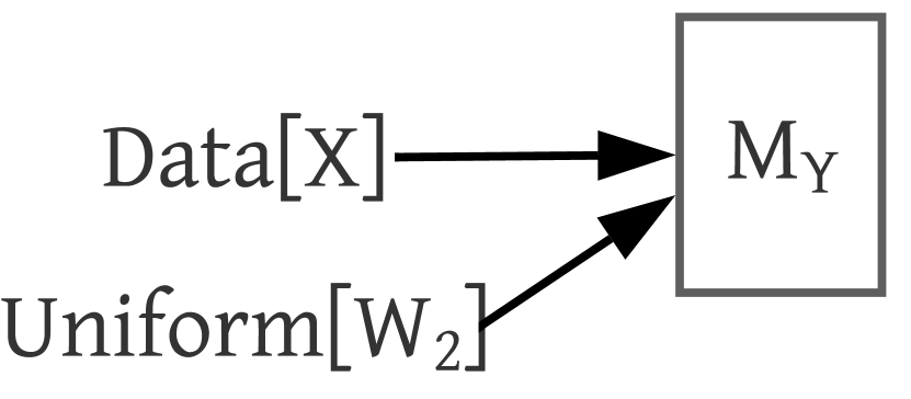
(e) Sampling network

Figure 14: ID-DAG (Section 4.2) causal graph simulation for the causal query $P_{w_{1}}(y)$. Causal graphs are before performing the corresponding step.

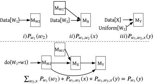
Figure 15: During the bottom up phase (Section 4.2), we combine the sampling networks corresponding to each c-component (top) into a single network $\mathcal{H}$ (bottom). For any $\text{do}(W_{1}=w_{1})$, we can use $\mathcal{H}$ to get samples from $P_{w_{1}}(y)$.

Algorithm simulation: To sample from $P_{w_{1}}(y)$ for the causal graph $G$ in Figure 14(a), we apply $\text{ID-DAG}(\mathbf{Y}=\{Y\},\mathbf{X}=\{W_{1}\},G,\mathcal{D},{\hat{\mathbf{X}}}=\emptyset,{\hat{{G}}}=G)$. Since $G\setminus\{W_{1}\}$ has three c-components $\{W_{2}\},\{X\},\{Y\}$, we first call ID-DAG step 4. $P_{w_{1}}(y)$ is factorized as: $\sum_{x,w_{2}}P_{w_{1},x,y}(w_{2})$ $P_{w_{1},w_{2},y}(x)$ $P_{w_{1},w_{2},x}(y)$. Thus, step 4 will return the sampling networks $\{H_{W_{2}},H_{X},H_{Y}\}$ that can sample from each of these factors. We focus on obtaining $H_{Y}$. ID-DAG reaches step 7 for the query: $P_{w_{1},w_{2},x}(y)$ since we have $S=G\setminus\{W_{1},W_{2},X\}=\{Y\},S^{\prime}=\{W_{1},X,Y\}$ and $S\subset S^{\prime}$ (Figure 14(b)). Here, sampling from $P_{x,w_{1},w_{2}}(y)$ in $G$, with observational training dataset is equivalent to sampling from $P_{x,w_{1}}(y)$ in ${\hat{{G}}}=G_{\overline{W_{2}}}$ with $\text{do}(W_{2})$ interventional data. With $W_{2}\sim P(w_{2})$, we generate $\mathcal{D}^{\prime}\sim P_{w_{2}}(\mathbf{v})$ by calling step 6 (base case). We pass $\mathcal{D}^{\prime}$ as the dataset parameter for the next recursive call. This step implies that if the recursive call returns a network that samples from $P_{x,w_{1}}(y)$, it can also be used to sample from $P_{w_{1},w_{2},x}(y)$.

In Figure 14(c), $W_{1}\notin An(Y)_{G}$. Thus, we drop $W_{1}$ from the all parameters before next recursive call. We are at the base case (Figure 14(d)) with ${\hat{{G}}}:W_{2}\rightarrow X\rightarrow Y$. Thus, we train a conditional model $M_{Y}(W_{2},X)$ on $\mathcal{D}^{\prime}[W_{2},X,Y]$ that can sample from $P(y|w_{2},x)$. This would be returned as $H_{Y}$ at step 4 (Figure 14(e)). Similarly, we can obtain sampling network $H_{W_{2}}$ and $H_{X}$ to sample from $P_{w_{1},x,y}(w_{2})=P(w_{2}|w_{1})$ and $P_{w_{1},w_{2},y}(x)=\sum_{w_{1}^{\prime}}P(x|w_{1}^{\prime},w_{2})P(w_{1}^{\prime})$. We connect these networks as shown in Figure 15.

Appendix F Appendix: Experimental Details

F.1 Napkin-MNIST Dataset

Data Generation: First we consider a synthetic dataset imbued over the napkin graph. We consider variables $W_{1},W_{2},X,Y$, where $W_{1},X,Y$ are images derived from MNIST and $W_{2}$ is a paired discrete variable. We introduce latent confounders $C,T$, denoting color and thickness, where $C$ can be any of $\{red,greed,blue,yellow,magenta,cyan\}$, and $T$ can be any of $\{thin,regular,thick\}$. Data generation proceeds as follows: first we sample latent $C,T$ from the uniform distribution. We color and reweight a random digit from MNIST to form $W_{1}$. $W_{2}$ only keeps the digit value in $\{0\dots 9\}$ of $W_{1}$ and a restriction of its color: if the color of $W_{1}$ is $red$, $green$, or $blue$, $W_{2}$’s color value is 0, and it is 1 otherwise. $X$ then picks a random MNIST image of the same digit as $W_{2}$’s digit value (0-9), is colored according to $W_{2}$’s color value (0-1), and is reweighted according to the latent $T$. Then $Y$ is the same original MNIST image as $X$, with the same thickness but colored according to the latent $C$. Further, for every edge in the graph, we include a random noising process: with probability $0.1$, the information passed along is chosen in a uniformly random manner from the valid range.

Here we describe the data-generation procedure, and training setup for the Napkin-MNIST experiment in full detail.

F.1.1 Data Generation Procedure: Discrete Case

As a warm-up, we outline the generation for the Napkin-MNIST dataset in a low-dimensional setting. When we consider in the next section the high-dimensional case, we simply replace some of these discrete variables with MNIST images which can be mapped back into this low-dimensional case.

We start by enumerating the joint distribution and the support of each marginal variable. First lets define the sets

• $\texttt{COLORS}:=\{\texttt{red, green, blue, yellow, magenta, cyan}\}$.

• $\texttt{RG\_COLORS}:=\{\texttt{red, green}\}$.

• $\texttt{THICKNESSES}:=\{\texttt{thin, regular, thick}\}$.

• $\texttt{DIGITS}:=\{0,\dots,9\}$.

And then the definitions and support of each of the variables in our distribution:

• (Latent) $\texttt{Color}\in\texttt{COLORS}$.

• (Latent) $\texttt{Thickness}\in\texttt{THICKNESSES}$.

• $W_{1}\in\texttt{DIGITS}\times\texttt{COLORS}\times\texttt{THICKNESSES}$

• $W_{2}\in\texttt{DIGITS}\times\texttt{RG\_COLORS}$.

• $X\in\texttt{DIGITS}\times\texttt{COLORS}\times\texttt{THICKNESSES}$

• $Y\in\texttt{DIGITS}\times\texttt{COLORS}\times\texttt{THICKNESSES}$

Now we describe the full data generation procedure. A key hyperparameter is a noise-probability $p$. This defines the probability that any variable flips to a uniform probability. To ease notation, we define the function $\eta_{p}(v,S)$ defined as

$$\eta_{p}(v,S):=\begin{cases}v&\text{with probability }1-p\\ U(S)&\text{otherwise }\end{cases}$$

and we define the mapping $R:\texttt{COLORS}\to\texttt{RESTRICTED\_COLORS}$ as

$$R(c):=\begin{cases}\texttt{red}&\text{if }c\in\{\texttt{red, green, blue}\}\\ \texttt{green}&\text{otherwise }\end{cases}$$

Where $U(S)$ means a uniformly random choice of $S$. Then our data generation procedure follows the following steps:

• $\texttt{Color}:=U(\texttt{COLORS})$

• $\texttt{Thickness}:=U(\texttt{THICKNESSES})$

• $W_{1}:=\big{(}U(\texttt{DIGITS}),\quad\eta_{p}(\texttt{Color},\texttt{COLORS}),\quad\eta_{p}(\texttt{Thickness},\texttt{THICKNESSES})\big{)}$

• $W_{2}:=\big{(}\eta_{p}(W_{1}._{digit},\texttt{DIGITS}),\quad\eta_{p}(R(W_{1}._{color},\texttt{RG\_COLORS})\big{)}$

• $X:=\big{(}\eta_{p}(W_{2}._{digit},\texttt{DIGITS}),\quad\eta_{p}(W_{2}._{color},\texttt{RG\_COLORS}),\quad\eta_{p}(\texttt{Thickness},\texttt{THICKNESSES})\big{)}$

• $Y:=\big{(}\eta_{p}(X._{digit},\texttt{DIGITS}),\quad\eta_{p}(\texttt{Color},\texttt{COLORS}),\quad\eta_{p}(X._{thickness},\texttt{THICKNESSES})\big{)}$

It is easy to verify that this describes the Napkin graph, as each only Color, Thickness are latent and each variable only depends on its parents in the SCM.

Secondly, observe that this structural causal model is separable with respect to digits, colors, and thicknesses. Since each digit only depends on parent digits, each color only depends on parent colors, and each thickness depends only on parent thicknesses, these can all be considered separately.

Further, because this distribution is only supported over discrete variables, exact likelihoods can be computed for any conditional query. This is much more easily done programmatically, however, and we provide code in the attached codebase to do just that. We will claim without proof that in the case of thicknesses and digits, $P_{Y}(X)=P(Y|X)$. However in the case of colors, $P_{Y}(X)\neq P(Y|X)$. Hence we consider this case in the evaluations in the experiments section.

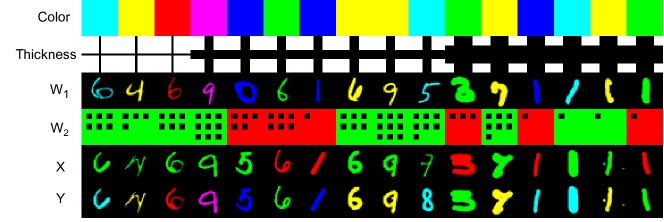
Figure 16: Joint samples from the Napkin-MNIST dataset: Samples from the Napkin-MNIST dataset are visualized as columns above. The first row indicates the latent variable color, the second row indicates the latent variable thickness, and the row labeled $W_{2}$ is a discrete variable holding a (color, digit), where digit is represented as the number of dots. Notice that the noising process sometimes causes information to not be passed to children.

F.1.2 Data Generation Procedure: High-dimensional case

The high-dimensional case follows the discrete case of the Napkin-MNIST dataset, with a few key changes. Namely, $W_{1},X,$ and $Y$ are MNIST images that have been colored and thickened. We explicitly outline these changes:

• $W_{1}$: A random MNIST image of the provided digit is used, then colored and thickened accordingly (noisy from latents).

• $W_{2}:$ This is a discrete variable, only encoding the (noised) digit and (noised) restricted color of $W_{1}$.

• $X$: This is a random MNIST image of the (noised) digit obtained from $W_{2}$, then colored with the (noised) restricted color from $W_{2}$ and thickened according to the (noised) latent thickness.

• $Y$: This is the same base image of $X$, unless the noising procedure calls for a change in digit, then a random MNIST image of the specified image is used. The (noisy) color is obtained from the latent distribution, and the (noisy) thickness is obtained from $X$.

To color the images, we convert each 1-channel MNIST image into a 3-channel MNIST image, and populate the necessary channels to generate these colors. Note that in RGB images: if only the RG channels are active, the image is yellow; if only the RB channels are active, the image is magenta; if only the BG channels are active, the image is cyan. To thicken the images, we use the MorphoMNIST Castro et al. (2019) package. Operationally, we generate a base dataset for our experiments of size equivalent to the original MNIST dataset. That is, the training set has a size of 60K, and the test set has a size of 10K. Because we have access to the latents during the data generation procedure, we are able to train classifiers for each variable to identify their digit, color and thickness. We use a simple convolutional network architecture for each of these cases and achieve accuracy upwards of 95% in each case.

F.1.3 Diffusion Training Details

We train two diffusion models during our sampling procedure, and we discuss each of them in turn.

To train a model to sample from $P_{(}X,Y|W_{1},W_{2})$, we train a single diffusion model over the joint $(X,Y)$ distribution, i.e., 6 channels. We train a standard UNet architecture where we follow the conditioning scheme of classifier-free guidance. That is, we insert at every layer an embedding of the $W_{1}$ (image) and $W_{2}$ (2-dimensional discrete variable). To embed the $W_{1}$ image, we use the base of a 2-layer convolutional neural network for MNIST images, and to embed the $W_{1}$ we use a standard one-hot embedding for each of the variables. All three embeddings are concatenated and mixed through a 2-layer fully connected network to reach a final embedding dimension of 64. Batch sizes of 256 are used everywhere. Training is performed for 1000 epochs, which takes roughly 9 hours on 2 A100 GPU’s. Sampling is performed using DDIM over 100 timesteps, with a conditioning weight of $w=1$ (true conditional sampling) and noise $\sigma=0.3$.

To train a model to sample $Y$ from the generated dataset $(W_{2},X,Y)$, we follow an identical scheme. An option is to train a single diffusion model for each choice of $W_{2}$ in our synthetic dataset, however, we argue our schema still produces correct samples because: 1) $W_{2}$ can be arbitrarily chosen, and thus should not affect $Y$, 2) we argue that the model fidelity benefits from weight sharing across multiple choices of $W_{2}$, 3) the model is only ever called with a specified value of $W_{2}$ so we always condition on this $W_{2}$.

F.1.4 Extra Evaluations

As such, our evaluations include verifying the quality of the trained component neural networks and, in the case of MNIST, a surrogate ground truth for a discrete version of the dataset. In each experiment, for conditional sampling with high-dimensional data, we train diffusion models using classifier-free guidance (Ho & Salimans, 2022). For conditional sampling of categorical data, we train a classifier using cross-entropy loss. In addition to the evaluations presented in the main paper, we can further perform evaluations on the component models necessary to sample $P_{X}(Y)$.

$P(X,Y|W_{1},W_{2})$:

We can evaluate the model approximating samples from $P(X,Y|W_{1},W_{2})$ on a deeper level than just visual inspection as provided in the main paper. In particular, assuming access to good classifiers that can predict the digit, color, and thickness of an MNIST image, we can compare properties of the generated images with respect to the ground truth in the discrete case. For example, assuming we have hyperparameter of random noise equal to $p$, we can compute the following quantities analytically on the discrete dataset as:

• $P[X_{d}={W_{2}}_{d}]=1-p+\frac{p}{10}$

• $P[X._{c}={W_{2}}_{c}]=1-p+\frac{p}{10}$

• $P[X_{t}={W_{1}}_{t}]=(1-p+\frac{p}{3})^{2}+\big{(}\frac{p}{3}\big{)}^{2}\cdot 2$

• $P[Y_{d}=X_{d}]=1-p+\frac{p}{10}$

• $P[Y_{c}={W_{1}}_{c}]=(1-p+\frac{p}{6})^{2}+big(\frac{p}{6}\big{)}^{2}\cdot 5$

• $P[Y_{t}=X_{t}]=1-p+\frac{p}{3}$

where $V_{d},V_{c},V_{t}$ refer to the digit, color, and thickness attributes respectively. These calculations follow from two formulas. In a discrete distribution with support $S$ and $|S|=K$:

• $P[\eta_{p}(z,S)=z]=1-p+\frac{p}{K}$

• $P[\eta_{p}(z,S)=\eta_{p}(z,S)]=(1-p+\frac{p}{K})^{2}+\Big{(}\frac{p}{K}\Big{)}^{2}\cdot(K-1)$

where in the second equation, it is assumed that $\eta_{p}(\cdot,\cdot)$ are two independent noising procedures.

Then to evaluate, we can 1) consider a large corpus of joint data, 2) run each of $W_{1},X,Y$ through a classifier for digit, color, and thickness, 3) evaluate the empirical estimate of each desired probability. We present these results for the synthetic dataset $D_{synth}$ sampled from the diffusion model approximating $P(X,Y|W_{1},W_{2})$, a dataset $D_{orig}$ generated according to the data generation procedure, and $P_{true}$ the true analytical probabilities. These results are displayed in the Table 2.

Table 2: Evaluations on the Napkin-MNIST generated dataset. $V.d,V.c,V.t$ refer to the digit, color and thickness respectively of variable $V$. The first column is with respect to samples generated from diffusion model $\hat{P}(X,Y\mid W_{1},W_{2})$, Image Data is the dataset used to train $\hat{P}$, Discrete Data is the empirical distribution according to a discrete Napkin-MNIST, and the ground truth is analytically computed. Ideally all values should be equal across a row. While our synthetic dataset generated from $\hat{P}$ is not a perfect representation, it is quite close in all attributes except thickness. This is because the classifier for thickness has some inherent error in it, as evidenced by the mismatch between the base data and ground truth in the thickness rows.

	$\hat{P}(Y,X\mid W_{1},W_{2})$	Image Data	Discrete Data	Ground Truth
$P[X.d=W_{2}.d]$	0.931	0.895	0.909	0.910
$P[X.c=W_{2}.c]$	0.964	0.950	0.950	0.950
$P[X.t=W_{1}.t]$	0.683	0.776	0.879	0.873
$P[Y.d=X.d]$	0.927	0.895	0.909	0.910
$P[Y.c=W_{1}.c]$	0.847	0.841	0.841	0.842
$P[Y.t=X.t]$	0.830	0.851	0.933	0.933

F.1.5 MNIST baseline comparison

Here we provide some additional information about the baseline comparison we showed in Section 5.1. Although the implementation of the baseline methods is different, we considered the performance of each method after running them for 300 epochs (until good image quality is obtained). The NCM algorithm took around 50 hours to complete while our algorithm took approximately 16 hours to complete. We observe the probabilities in Table 3.

In the generated samples from the conditional model, the color of digit image $X$ and digit image $Y$ are correlated due to confounding through backdoor paths. For example, for a digit image $X$ with color as red, $Y$ takes a value from [Red, Green, Blue] with high probability. Thus, the conditional model does not have the ability to generate interventional samples. On the other hand, our algorithm generates samples from the interventional distribution $P(y|\text{do}(x))$ and the generated samples choose different colors:[Red, Green, Blue, Yellow, Magenta, Cyan] with almost the same probability. Therefore, our algorithm shows superior performance compared to baselines and illustrates the high-dimensional interventional sampling capability.

Table 3: Color probability distribution of the sampled images. $P(y.c|x.c=red)$ is biased towards [R,G,B] while $P(y.c|do(x.c=red))$ is not.

Predicted color probabilities	Red	Green	Blue	Yellow	Magenta	Cyan
Conditional model: $P(y.c|x.c=red)$	0.1889	0.4448	0.1612	0.1021	0.0232	0.0798
Ours: $P(y.c|do(x.c=red))$	0.1278	0.2288	0.2097	0.1445	0.1177	0.1715

F.2 CelebA Experiment

Here we provide some additional information about the CelebA image to image translation experiment we showed in Section 5.2. We used a pre-trained classifier from this repository: https://github.com/clementapa/CelebFaces_Attributes_Classification. We use the pre-trained model of EGSDE from this repository:https://github.com/ML-GSAI/EGSDE We use the pre-trained model of StarGAN from this repository:https://github.com/yunjey/stargan. Note that although EGSDE generates better quality (blur-free) images compared to StarGAN (blurry), it makes its samples more realistic by adding different non-causal attributes such as $Young$ or $Attractive$. As a result, it will generate $Female$ samples from a specific part of the image manifold. As a result, it might lack the ability to generate a different variety of images (for example: old females). The reason behind this is possibly the correlation in the dataset it is trained on. For example, in the CelebA dataset, we observe a high correlation between $Female$ and $Young$ while also a high correlation between $Male$ and $Old$. As a result, when EGSDE converts the images whether the Male is young or old, it converts them to a young female. On the other hand, starGAN does not change noncausal attributes, but it also does not properly change the causal attributes as well.

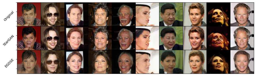
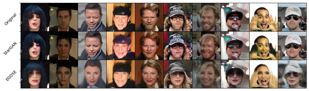
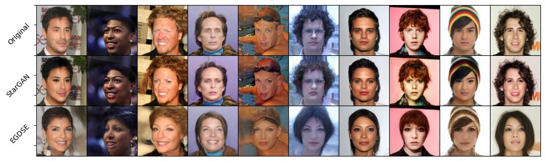
Figure 18: Performance comparison of multi-domain image translation between StarGAN and EGSDE.

Table 4: Additional attributes added (in percentage) in the translated images.

	WearingLipstick	HeavyMakeup	ArchedEyebrows	OvalFace	Attractive	Young
Added Attribute (%)	87.5	79.16	66.66	54.16	37.5	29.16

F.2.1 Conditional image generation

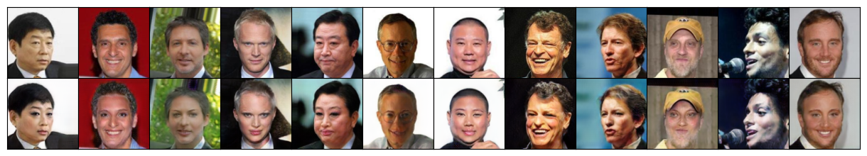
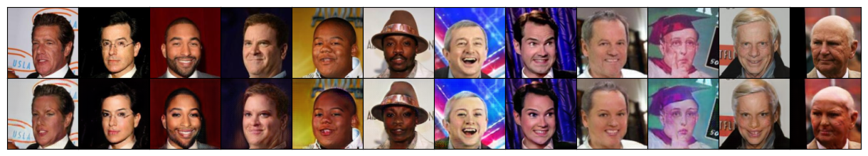
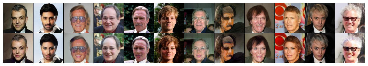
Figure 19: Samples from $P(I_{2}|Young=1,\text{do}(Male=0))$ generated by StarGAN.

F.3 Covid X-Ray Dataset

F.3.1 Data Preprocessing

Note that a full pipeline of data preparation is contained in cxray/prep_cxray_dataset.sh in the provided codebase. We start by downloading the corpus approximately 30K Covid X-Ray images. Then we download Covid-19 labels and Pneumonia labels and attach labels to each image. Then we convert each image to black-white one-channel images and rescale each to a size of $(128\times 128)$ pixels. Finally, a random split of the 30K images is performed: keeping 20K to be used during training, and 10K to be used as validation images. Note that the labels come with a set of 400 test images, but 400 images is too small to be an effective test set (say for FID computations). We will be explicit about where we use each data set.

F.3.2 Diffusion Training Details

We train a diffusion model to approximate $P(X|C)$. To do this, we use a standard UNet and classifier-free guidance scheme. We train for 100K training steps over the 20K-sized training set, using a batch size of 16. This takes roughly 10 hours on a single A100. The same classifier-free guidance parameters are used as in the NapkinMNIST diffusion training.

F.3.3 Calibrated Classifier Training Details

To train a classifier to sample from $P(N|C,X)$, we note that our inputs are a $(1,128,128)$ image and a binary variable. Our architecture is as follows: we create an embedding of $X$ by modifying the final linear layer of a ResNet18 to have output dimension 64 (vs 1000), and modify the input channels to be 1. We create an embedding for $N$ by using a standard embedding layer for binary variables, with embedding dimension 64. These embeddings are then concatenated and pushed through 3 fully connected layers with ReLU nonlinearities and dimension 128. A final fully-connected layer with 2 outputs is used to generate logits.

Training follows a standard supervised learning setup using cross entropy loss. We train for 100 epochs using a batch size of 256 and a standard warmup to decaying learning rate (see code for full details).

We note the deep literature suggesting that even though classifiers seek to learn $P(N|X,C)$, neural networks trained using cross entropy loss do not actually do a very good job of estimating this distribution. Training attains an accuracy of $91.2\%$ on the test set. Calibrated classification seeks to solve this problem by modifying the network in a way such that it more accurately reflects this distribution. We follow the standard approach using temperature scaling of the logits, where a temperature is learned over the validation set, using LBFGS with a learning rate of 0.0001 and a maximum of 10K iterations. This does not affect the test accuracy at all, but drastically improves the ECE and MCE reliability metrics. See Guo et al. (2017) for a further discussion of temperature scaling.

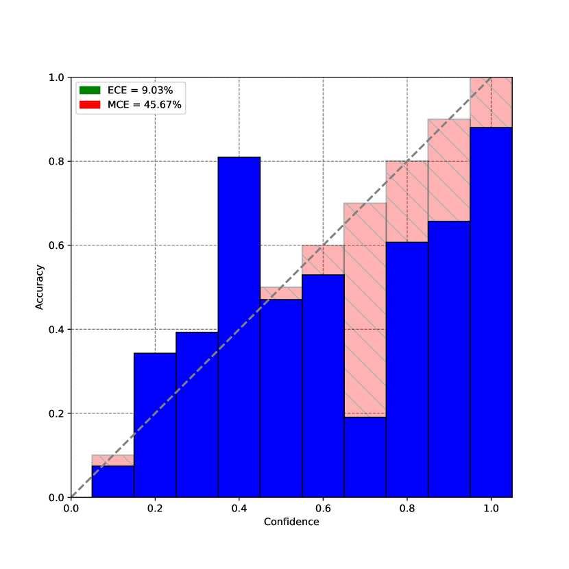
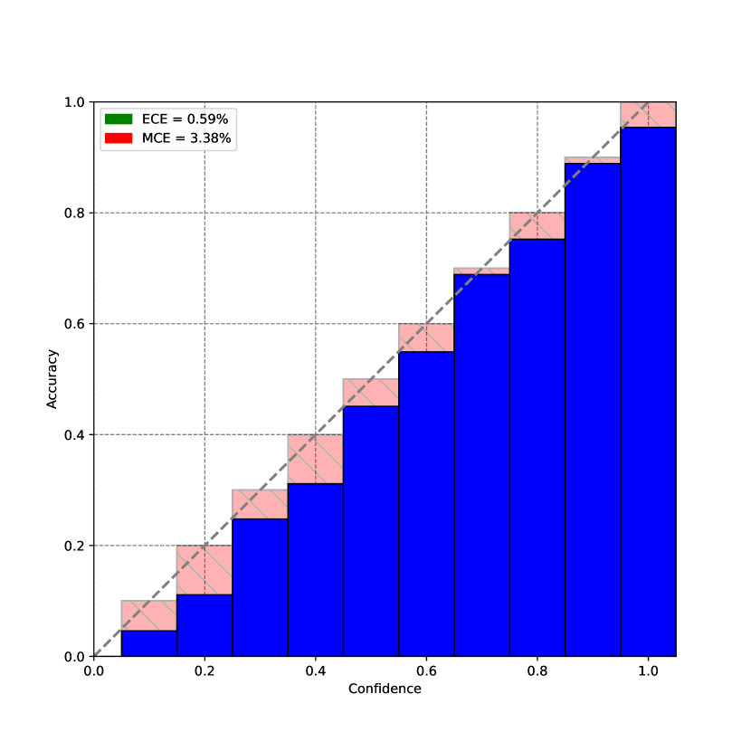
Figure 20: Reliability plots for $\mathbf{P(N|C,X)}$:. Reliability plots which overlay accuracy versus classifier confidence. (Left) Reliability plot for $P(N|C,X)$ without calibration. (Right) Reliability plot for $P(N|C,X)$ with temperature scaling calibration applied.

Appendix G Miscellaneous

The causal graph in Figure 1 used to compare different related works was motivated from Ribeiro et al. (2023).

References

- Balazadeh Meresht et al. (2022) Balazadeh Meresht, V., Syrgkanis, V., and Krishnan, R. G. Partial identification of treatment effects with implicit generative models. Advances in Neural Information Processing Systems, 35:22816–22829, 2022.
- Bareinboim & Pearl (2012) Bareinboim, E. and Pearl, J. Causal inference by surrogate experiments: z-identifiability. In Proceedings of the Twenty-Eighth Conference on Uncertainty in Artificial Intelligence, pp. 113–120, 2012.
- Castro et al. (2019) Castro, D. C., Tan, J., Kainz, B., Konukoglu, E., and Glocker, B. Morpho-mnist: quantitative assessment and diagnostics for representation learning. Journal of Machine Learning Research, 20(178):1–29, 2019.
- Chao et al. (2023) Chao, P., Blöbaum, P., and Kasiviswanathan, S. P. Interventional and counterfactual inference with diffusion models. arXiv preprint arXiv:2302.00860, 2023.
- Choi et al. (2018) Choi, Y., Choi, M., Kim, M., Ha, J.-W., Kim, S., and Choo, J. Stargan: Unified generative adversarial networks for multi-domain image-to-image translation. In Proceedings of the IEEE Conference on Computer Vision and Pattern Recognition, 2018.
- Croitoru et al. (2023) Croitoru, F.-A., Hondru, V., Ionescu, R. T., and Shah, M. Diffusion models in vision: A survey. IEEE Transactions on Pattern Analysis and Machine Intelligence, 2023.
- Goyal et al. (2019) Goyal, Y., Feder, A., Shalit, U., and Kim, B. Explaining classifiers with causal concept effect (cace). arXiv preprint arXiv:1907.07165, 2019.
- Guo et al. (2017) Guo, C., Pleiss, G., Sun, Y., and Weinberger, K. Q. On calibration of modern neural networks, 2017.
- Ho & Salimans (2021) Ho, J. and Salimans, T. Classifier-free diffusion guidance. In NeurIPS 2021 Workshop on Deep Generative Models and Downstream Applications, 2021.
- Ho & Salimans (2022) Ho, J. and Salimans, T. Classifier-free diffusion guidance. arXiv preprint arXiv:2207.12598, 2022.
- Ho et al. (2020) Ho, J., Jain, A., and Abbeel, P. Denoising diffusion probabilistic models. Advances in Neural Information Processing Systems, 33:6840–6851, 2020.
- Jaber et al. (2018) Jaber, A., Zhang, J., and Bareinboim, E. Causal identification under markov equivalence. arXiv preprint arXiv:1812.06209, 2018.
- Jung et al. (2020) Jung, Y., Tian, J., and Bareinboim, E. Learning causal effects via weighted empirical risk minimization. Advances in neural information processing systems, 33:12697–12709, 2020.
- Karras et al. (2019) Karras, T., Laine, S., and Aila, T. A style-based generator architecture for generative adversarial networks. In Proceedings of the IEEE/CVF conference on computer vision and pattern recognition, pp. 4401–4410, 2019.
- Kocaoglu et al. (2018) Kocaoglu, M., Snyder, C., Dimakis, A. G., and Vishwanath, S. Causalgan: Learning causal implicit generative models with adversarial training. In International Conference on Learning Representations, 2018.
- Lee et al. (2020) Lee, S., Correa, J. D., and Bareinboim, E. General identifiability with arbitrary surrogate experiments. In Uncertainty in artificial intelligence, pp. 389–398. PMLR, 2020.
- Liu et al. (2015) Liu, Z., Luo, P., Wang, X., and Tang, X. Deep learning face attributes in the wild. In Proceedings of International Conference on Computer Vision (ICCV), December 2015.
- Louizos et al. (2017) Louizos, C., Shalit, U., Mooij, J. M., Sontag, D., Zemel, R., and Welling, M. Causal effect inference with deep latent-variable models. Advances in neural information processing systems, 30, 2017.
- Maathuis & Colombo (2015) Maathuis, M. H. and Colombo, D. A generalized back-door criterion. The Annals of Statistics, 43(3):1060, 2015.
- Pawlowski et al. (2020) Pawlowski, N., Coelho de Castro, D., and Glocker, B. Deep structural causal models for tractable counterfactual inference. Advances in Neural Information Processing Systems, 33:857–869, 2020.
- Pearl (1980) Pearl, J. Causality: models, reasoning, and inference, 1980.
- Pearl (1993) Pearl, J. [bayesian analysis in expert systems]: comment: graphical models, causality and intervention. Statistical Science, 8(3):266–269, 1993.
- Pearl (1995) Pearl, J. Causal diagrams for empirical research. Biometrika, 82(4):669–688, 1995.
- Pearl (2009) Pearl, J. Causality. Cambridge university press, 2009.
- Rahman & Kocaoglu (2024) Rahman, M. M. and Kocaoglu, M. Modular learning of deep causal generative models for high-dimensional causal inference. arXiv preprint arXiv:2401.01426, 2024.
- Ribeiro et al. (2023) Ribeiro, F. D. S., Xia, T., Monteiro, M., Pawlowski, N., and Glocker, B. High fidelity image counterfactuals with probabilistic causal models. arXiv preprint arXiv:2306.15764, 2023.
- Rosenbaum & Rubin (1983) Rosenbaum, P. R. and Rubin, D. B. The central role of the propensity score in observational studies for causal effects. Biometrika, 70(1):41–55, 1983.
- Sanchez & Tsaftaris (2022) Sanchez, P. and Tsaftaris, S. A. Diffusion causal models for counterfactual estimation. arXiv preprint arXiv:2202.10166, 2022.
- Shalit et al. (2017) Shalit, U., Johansson, F. D., and Sontag, D. Estimating individual treatment effect: generalization bounds and algorithms. In International conference on machine learning, pp. 3076–3085. PMLR, 2017.
- Shen et al. (2020) Shen, Y., Gu, J., Tang, X., and Zhou, B. Interpreting the latent space of gans for semantic face editing. In Proceedings of the IEEE/CVF conference on computer vision and pattern recognition, pp. 9243–9252, 2020.
- Shpitser & Pearl (2008) Shpitser, I. and Pearl, J. Complete identification methods for the causal hierarchy. Journal of Machine Learning Research, 9:1941–1979, 2008.
- Song et al. (2020) Song, J., Meng, C., and Ermon, S. Denoising diffusion implicit models. arXiv preprint arXiv:2010.02502, 2020.
- Subbaswamy et al. (2021) Subbaswamy, A., Adams, R., and Saria, S. Evaluating model robustness and stability to dataset shift. In International Conference on Artificial Intelligence and Statistics, pp. 2611–2619. PMLR, 2021.
- Tian (2002) Tian, J. Studies in causal reasoning and learning. University of California, Los Angeles, 2002.
- Tian & Pearl (2002) Tian, J. and Pearl, J. A general identification condition for causal effects. eScholarship, University of California, 2002.
- Vo et al. (2022) Vo, T. V., Bhattacharyya, A., Lee, Y., and Leong, T.-Y. An adaptive kernel approach to federated learning of heterogeneous causal effects. Advances in Neural Information Processing Systems, 35:24459–24473, 2022.
- Wang & Kwiatkowska (2023) Wang, B. and Kwiatkowska, M. Compositional probabilistic and causal inference using tractable circuit models. In International Conference on Artificial Intelligence and Statistics, pp. 9488–9498. PMLR, 2023.
- Wang et al. (2020) Wang, L., Lin, Z. Q., and Wong, A. Covid-net: a tailored deep convolutional neural network design for detection of covid-19 cases from chest x-ray images. Scientific Reports, 10(1):19549, Nov 2020. ISSN 2045-2322. doi: 10.1038/s41598-020-76550-z. URL https://doi.org/10.1038/s41598-020-76550-z.
- Xia et al. (2021) Xia, K., Lee, K.-Z., Bengio, Y., and Bareinboim, E. The causal-neural connection: Expressiveness, learnability, and inference. Advances in Neural Information Processing Systems, 34:10823–10836, 2021.
- Xia et al. (2023) Xia, K. M., Pan, Y., and Bareinboim, E. Neural causal models for counterfactual identification and estimation. In The Eleventh International Conference on Learning Representations, 2023. URL https://openreview.net/forum?id=vouQcZS8KfW.
- Xin et al. (2022) Xin, Y., Tagasovska, N., Perez-Cruz, F., and Raubal, M. Vision paper: causal inference for interpretable and robust machine learning in mobility analysis. In Proceedings of the 30th International Conference on Advances in Geographic Information Systems, pp. 1–4, 2022.
- Zečević et al. (2021) Zečević, M., Dhami, D., Karanam, A., Natarajan, S., and Kersting, K. Interventional sum-product networks: Causal inference with tractable probabilistic models. Advances in neural information processing systems, 34:15019–15031, 2021.
- Zhang et al. (2020) Zhang, C., Zhang, K., and Li, Y. A causal view on robustness of neural networks. Advances in Neural Information Processing Systems, 33:289–301, 2020.
- Zhang et al. (2021) Zhang, W., Liu, L., and Li, J. Treatment effect estimation with disentangled latent factors. In Proceedings of the AAAI Conference on Artificial Intelligence, volume 35, pp. 10923–10930, 2021.
- Zhao et al. (2022) Zhao, M., Bao, F., Li, C., and Zhu, J. Egsde: Unpaired image-to-image translation via energy-guided stochastic differential equations. arXiv preprint arXiv:2207.06635, 2022.