An Interpretable Low-complexity Model for Wireless Channel Estimation

Abstract

With the advent of machine learning, there has been renewed interest in the problem of wireless channel estimation. This paper presents a novel low-complexity wireless channel estimation scheme based on a tapped delay line (TDL) model of wireless signal propagation, where a data-driven machine learning approach is used to estimate the path delays and gains. Advantages of this approach include low computation time and training data requirements, as well as interpretability since the estimated model parameters and their variance provide comprehensive representation of the dynamic wireless multipath environment. We evaluate this model’s performance using Matlab’s ray-tracing tool under static and dynamic conditions for increased realism instead of the standard evaluation approaches using statistical channel models. Our results show that our TDL-based model can accurately estimate the path delays and associated gains for a broad-range of locations and operating conditions. Root-mean-square estimation error remained less than $10^{-4}$, or $-40$dB, for SNR $\geq 30$dB in all of our experiments.

The key motivation for the novel channel estimation model is to gain environment awareness, i.e., detecting changes in path delays and gains related to interesting objects and events in the field. The channel state with multipath delays and gains is a detailed measure to sense the field than the single-tap channel state indicator calculated in current OFDM systems.

I Introduction

The extraordinary success of data-driven machine learning techniques in estimating complex and non-linear system dynamics has led to the development of novel wireless channel estimation (CE) and management approaches [1, 2, 3, 4, 5, 6, 7, 8, 9, 10]. However, machine learning (ML)-based channel estimation models require substantial time and data for training, which makes them unsuitable for real-time applications. Moreover, they are generally black-box, or non-interpretable, and the complex patterns learned by the model cannot be used to derive key insights about the radio environment. In this paper, we propose a “gray-box” approach, where we use a mathematical model to represent the channel and learn its parameters through a ML-inspired data-driven approach. Our results show that this approach not only provides better channel estimation than conventional methods, such as Least Squares, but the estimated channel state is a more detailed measure to sense the field in an environment awareness application. In our results section, we have also included a preliminary case study of drone detection using our channel estimation model with existing wireless signals.

The basic element of our approach is a Tapped-Delay Line (TDL) model of the wireless channel. A TDL model represents the received signal as a superposition of input signals traversing through line-of-sight or reflected from various objects in the environment, each experiencing different delays and attenuation. Due to movement of the mobile user or objects in the environment, the number of these multipaths, their delays, and gains change with time, which makes it extremely difficult to estimate and measure them accurately.

ITU’s (International Telecommunication Union) recommendations for parameterization of multipath environments use power thresholds to determine the number of multipath components. Not meant for real-time CE, ITU recommendations are for characterization of different scenarios. Some efforts using ML have also been proposed, e.g., [11] models the tap and gain estimation problem as multi-class classification using deep neural network and requires training of the model by a dictionary of channel models. This work improves the CE performance of a previous method [12] which formulates the estimation of taps, for specific transmitted and received signals in a Multi-Input Multi-Output (MIMO) system, as an optimization problem.

Among more general CE approaches, i.e., not using a TDL model, notable works are [2, 4], which use Generative Adversarial Networks (GANs), and [7], which incorporates variational autoencoders, to estimate the distribution of received signals or the channel impulse response of time varying channels. A large body of work in CE focuses on the problem of extrapolating channel estimates for all operating frequencies and times in an OFDM MIMO system, when the actual CE estimates are based on a handful of pilot symbols, mostly calculated by classical single-tap methods, such as least squares. Compressed sensing is one of the earlier solutions and most ML-based methods consider it as a baseline, such as, Approximate Message Passing [1], deep image processing and image restoration [3], attention based encoder-decoder [6, 9], unfolded neural networks [8], and GANs [1, 5]. Noting the issue of computation time, recent works suggest bi-directional RNN [10] and [13] recommends transfer learning and federated/split/distributed learning to speed up the CE process.

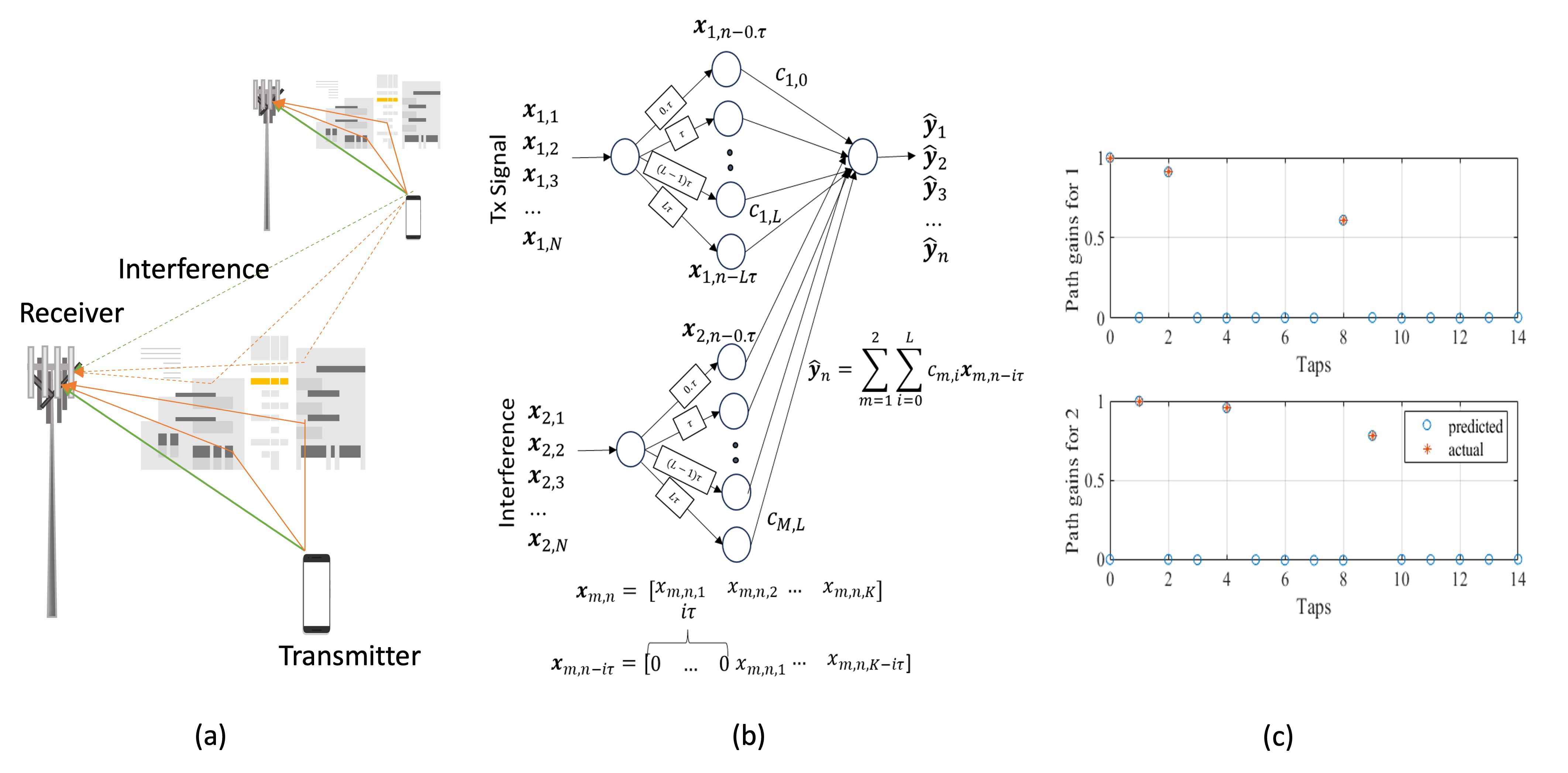
Figure 1: A small example of a single transmitter and receiver pair with one in-band interferer. We assume time-invariant multipaths in this example. (a) scenario, (b) TDL-NN CE model, and (c) CE results and actual path gains using Matlab simulations.

This paper focuses on the problem of CE using transmitted and received signals leveraging the respective strengths of classical and ML techniques, which can provide an approach for performing CE in real-time and can also facilitate environment awareness where objects and events of interest in the field can be detected by detecting changes in estimated channel states. In particular, our contributions are as follows:

• We propose a novel low-complexity data-driven channel estimation approach based on a neural network with one hidden layer using the reference signals already available in wireless communication systems.

• We evaluate the CE model using Matlab’s ray-tracing tool instead of the classical approach of employing statistical channel models, for increased realism.

• Our CE model shows accurate estimation (root-mean-square error is under $10^{-4}$), or $-40$dB for different static and dynamic scenarios with reasonable SNR ($\geq 30$dB).

• We also show the potential of our CE model in finding outlier events in the neighbourhood of the transmitter and receiver.

II System Model

The signal from a wireless transmitter can be represented as [14]:

$$x(t)=\operatorname{Re}\{s(t)e^{j2\pi f_{c}t}\},$$

where $s(t)$ is the baseband signal and $f_{c}$ is the carrier frequency. The discrete time versions of the baseband and transmitted signal are $\textbf{{s}}_{n}$ and $\textbf{{x}}_{n}$ respectively, both vectors of length $K$. Considering that the signal will reach the receiver through line-of-sight and various reflected paths, which experience different Doppler shifts, the received signal $y(t)$ can be written as [14],

$$y(t)=\operatorname{Re}\left\{\sum_{i=0}^{D(t)-1}{c_{i}(t)s(t-\tau_{i}(t))e^{j(2\pi f_{c}(t-\tau_{i}(t))+{\phi}_{i}(t))}+w(t)}\right\},$$

where $c_{i}(t)$, $\tau_{i}(t)$, and ${\phi}_{i}(t)$ are the gain, delay, and Doppler shift of the $i$th path, $i=0$ corresponds to the line-of-sight and there are $D(t)$ distinct multipaths. $w(t)$ is the white Gaussian noise. In a time varying channel model, the parameters $\{c_{i}(t),\tau_{i}(t),{\phi}_{i}(t)\}~{}\forall{i}$, and $D(t)$ are random processes. The channel impulse response can be written as

$$h(\theta_{h}(t))=\sum_{i=0}^{D(t)-1}{c_{i}(t)\delta(t-\tau_{i}(t))e^{j{\phi}_{i}(t)}},$$ (1)

where $\theta_{h}(t)$, the parameters to describe channel impulse response are defined as

$$\theta_{h}(t)=\{c_{i}(t),\tau_{i}(t),{\phi}_{i}(t)\},~{}i=0,\cdots,D(t).$$ (2)

As can be seen in the above expression, the total phase shift experienced by the signal is $-2\pi f_{c}\tau_{i}(t)+{\phi}_{i}(t)$ due to multipaths and Doppler effect. The discrete time received signal and received baseband signal are denoted by $\textbf{{y}}_{n}$ and $\textbf{{z}}_{n}$ respectively, which are also considered as $K$ length vectors.

II-A An Illustrative Example

Before formally presenting our CE approach, we illustrate the underlying concept with the help of a small example as shown in Fig. 1. In Fig. 1a, there is a single transmitter/receiver pair with one in-band interferer or unintended signal leakage. For this case, CE is reduced to estimating $\theta_{h}=\{c_{i},\tau_{i}\},~{}\forall i$. We assume we have $N$ samples of transmitted signals, $\textbf{{x}}_{1,n}$ from the primary transmitter and $\textbf{{x}}_{2,n}$ from the interferer, and the associated received signal samples $\textbf{{y}}_{n}$, also given as

$$\textbf{{y}}_{n}=\sum_{i=0}^{D_{1}}c_{1,i}\textbf{{x}}_{n-\tau_{1,i}}+\sum_{i=0}^{D_{2}}c_{2,i}\textbf{{x}}_{2,n-\tau_{2,i}}+\textbf{{w}}_{n},$$

where $D_{1}$ and $D_{2}$ are the numbers of multipaths and $\textbf{{w}}_{n}$ is the white Gaussian noise.

Figure 1b shows our approach for estimating the path delays and gains. The basic unit of our model, called TDL-NN, is a neural network (NN) with a single input and single output and one hidden layer representing $L$ taps of constant delays in multiples of $\tau$. The parameters $L$ and $\tau$ should cover all possible distinct path delays. The output layer weights represent path gains and are learned iteratively by minimizing the MSE (Mean Square Error) loss function, i.e.,

$$\frac{1}{N}\sum_{n=1}^{N}\|\textbf{{y}}_{n}-\hat{\textbf{{y}}}_{n}\|^{2}_{2},$$

where $\hat{\textbf{{y}}}_{n}=\sum_{m=1}^{2}\sum_{i=0}^{L}c_{m,i}\textbf{{x}}_{m,n-i\tau}$.

Using Matlab, we simulated the scenario of $N=10^{4}$ transmitted symbols, with $20$ samples per symbol and each sample duration is $100$ns, $\tau_{1,i}=\{0,200,800\}$ns, $\tau_{2,i}=\{100,300,900\}$ns. Both transmitters use QPSK modulation, carrier frequency is 3MHz, and Gaussian noise is added with SNR of 15dB. Figure 1c shows the actual tap gains and the predicted gains from the PyTorch implementation of the model with delay resolution $\tau=100$ns and $L=15$. It can be seen that our TDL neural network accurately learned the path gains and delays. Our model uses a block size of $10^{4}$, $5000$ epochs, and the Adam optimizer with learning rate of $0.01$.

III TDL-NN Channel Estimation Approach

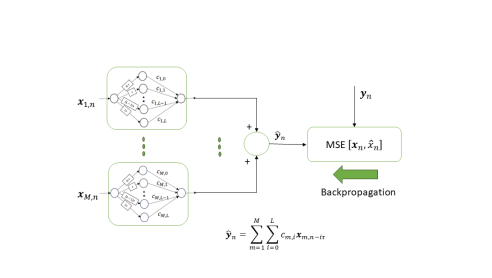
Figure 2: TDL-NN channel estimation for a scenario with multiple transmitters and one receiver.

In this section, we formally present our TDL neural network approach for channel estimation. All wireless communication systems use pilots or reference signals, which are known sequences of symbols transmitted over the wireless channel and the respective received signals are used for channel state estimation. Figure 2 shows $\textbf{{x}}_{m,n}$ transmitted reference signals from one primary transmitter and $M-1$ multiple interferers. The received reference signal is $\textbf{{y}}_{n}$. Our CE model is trained using $\textbf{{x}}_{m,n}$ and $\textbf{{y}}_{n}$ for $m={1,~{}\cdots,~{}M}$ and $n={1,~{}\cdots,~{}N}$, where $N$ is the available reference symbols for training.

The model shifts each input or transmitted signal, $\textbf{{x}}_{m,n}$, from $0\times\tau$ to $L\times\tau$, where $\tau$ is the tap delay resolution in the hidden layer. It then computes the weights of the output layers, or coefficients $c_{m,i}$ for all taps and also for all $M$ sub-models, by minimizing the MSE loss function as shown in the Fig. 2. Our implementation in PyTorch uses $N$ as the block-size and a learning rate of $0.01$. The computation complexity of our model grows as $\mathcal{O}(N\times L\times e)$, where $e$ is the number of epochs. As an option, we also implemented weight pruning in our model to push the smaller weights to 0. Note that our model uses the time shift idea as in conventional time delay neural networks [15], which were proposed for time series analysis, but otherwise it is a customized model to suit our application of channel estimation.

Path delays and gains change with time as mobile users or objects in the environment move. Weather conditions, such as, rain, wind, etc., also impact path gain. For a dynamic environment, the multipath delays and gains should be updated as new pilot symbols are received. Figure 2 shows one snapshot of our approach, which estimates $c_{m,i}(n)$ for each path tap $i$ at time $n$ by updating the model weights using pilot transmitted and received signals $\textbf{{x}}_{m,n}$ and $\textbf{{y}}_{n}$. Note that we are not explicitly estimating Doppler phase shift $\phi_{i}(t)$ associated with the path $i$ from the model, instead tracking the variations in path delays and gains.

Moreover, we remark that our TDL neural network is a realization of a typical Steepest Gradient Descent (SGD) algorithm iteratively computing coefficients of a linear predictor when the objective function is to minimize mean square error between actual observations and predictions. However, using SGD in a neural network setting with parallelization of computations is much more effective and an order of magnitude faster than the conventional iterative approach.

Furthermore, in systems using OFDM modulation, such as 4/5G or LTE, reference signals or pilots are embedded in subframes along with the payload. Channel estimation requires these pilots to be extracted first and then used to estimate the channel. In this case, baseband signals can be used for CE instead of transmitted or received signals with a carrier.

IV Experimental Results

IV-A Ray-tracing Simulations

In order to validate our TDL-based CE approach, we used Matlab’s ray-tracing tool to generate received signal data. To the best of our knowledge, this is the first CE paper which uses ray-tracing data for validation. Prior approaches have used statistical channel models, such as Rayleigh or Rician models, to generate the data [2, 4]. Use of ray-tracing not only allows us to assess the performance of our CE method by comparing it with the ground truth, it also facilitates testing the model efficacy under a wide-range of practical scenarios.

IV-A1 Static Multipath Scenario

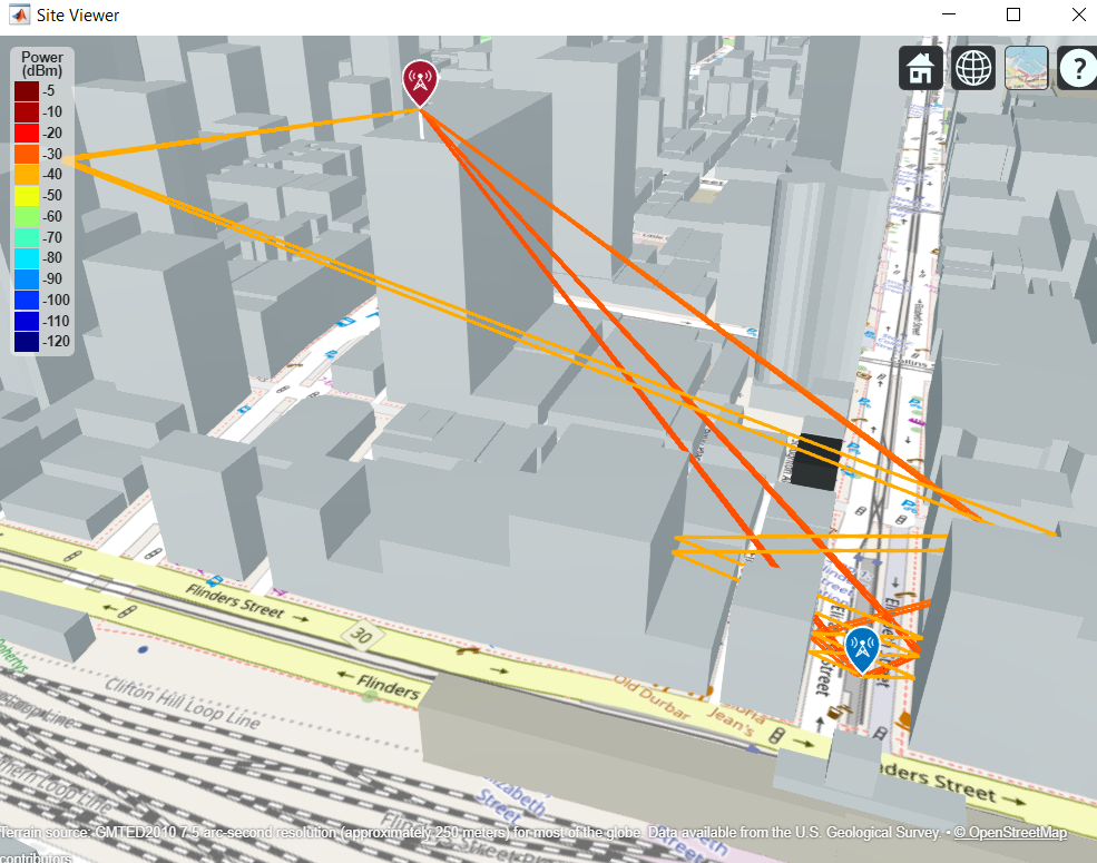
(a)

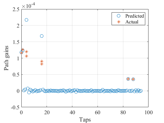
(b)

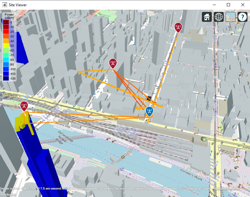
(c)

(d)

Figure 3: Static multipath scenario, (a) scene with one transmitter and receiver, (b) actual and estimated path delays and gains, taps 5 and 17 have 2 different rays and the estimation shows the combined effect, (c) scene of (a) with two interferers, (d) estimation error versus SNR for scenarios of one transmitter with no interferer (1 tx), one interferer (2 txs), and 2 interferers (3 txs).

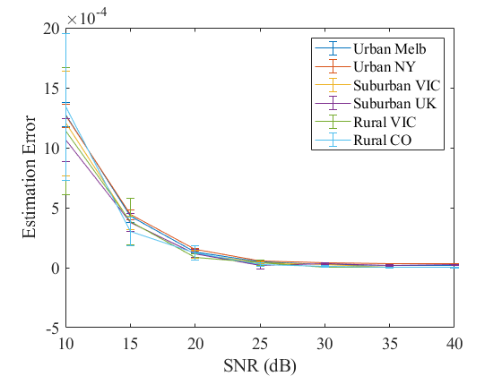
Figure 4: Estimation error versus SNR of TDL-NN channel estimation model in different urban, suburban, and rural scenarios.

We placed a transmitter and receiver in the Melbourne Central Business District scenario as shown in Fig. 3a. The transmitter is configured to transmit QPSK modulated signal with $900$MHz carrier frequency and $50$dBm power. It is placed at a height of 10m on the roof of a tall building and uses a directional antenna with azimuth angle of 30°. The receiver antenna’s angle is selected as 120°, and it is at a height of 1m from the ground as shown in Fig. 3a.

The maximum number of reflections in Matlab’s ray-tracing tool can be set as 10 (R2023b). Here, the tool finds 8 paths to the receiver. White Gaussian noise is added to the faded signal with SNR of $30$dB. The signal is amplified by $20$dB on reception. $10,000$ symbols, with $100$ samples per symbol, are generated and transmitted through the multipath channel. Each sample duration is $20$ns corresponding to a sampling frequency of $5\times 10^{7}$ samples/second. Unless otherwise stated, all the experiments in this paper uses the same configurations.

As shown in Fig. 3b, our TDL-NN model accurately finds channel taps and gains. Taps 5 and 17 show discrepancies, but the estimated gain is the collective impact of two rays with the same path delay. With weight pruning, smaller tap coefficients can be pushed to 0. However, for an unknown or time varying channel, this may not be advisable.

We also calculated the RMS (Root Mean Square) estimation error for different SNR conditions, as shown in Fig. 3d. Here, each point is averaged over 10 different estimation runs with $10,000$ training samples. In a high noise environment, the estimation error becomes excessive. We added interferers in our example as shown in Fig. 3c and estimated path delays and gains for all transmitted signals. As expected, the presence of multiple transmitters worsens the estimation error, however, the estimation accuracy of TDL-NN model remains high, for reasonable SNR, despite the presence of in-band interference.

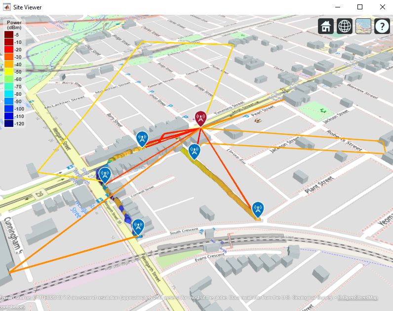
(a)

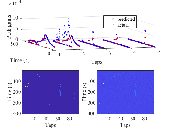
(b)

Figure 5: Changes in signal multipaths as the mobile user moves around a city block, (a) scene with changing rays when the receiver is at different locations, and (b) actual and estimated path delays and gains.

Figure 4 shows the estimation error vs. SNR plots for two urban scenarios (Melbourne Central Business District, Victoria, Australia and Manhattan, NY, USA), two suburban scenarios (Mount Waverley, Victoria, Australia and Chapelford, UK), and two rural areas (Wodonga, Victoria, Australia and Golden, CO, USA). The urban scenarios are more challenging due to the number of multipaths, whereas suburban areas have comparatively smaller number of reflections, but line-of-sight may be obstructed. Also, path attenuation may be excessive due to larger distances between users and base-stations in a sparse coverage situation. Rural areas on the other hand have mostly just the line-of-sight. Our TDL based CE approach performs exceptionally well for all conditions for reasonable SNR conditions as shown in Fig. 4.

IV-A2 Mobile Receiver Scenario

In this experiment, we picked an open-access GPS track of a walker around a block of streets, representing a receiver, as shown in Fig. 5a. Here a transmitter is placed 10m above the roof of a nearby building. Other configurations are the same as the static scenario. The colours of the GPS track shows the signal strength at that location, Figure 5a shows the receiver at multiple locations during the walk and changing multipath conditions.

This track has 405 points, sampling walker’s location every second. We generated $1000$ transmitted symbols for each location, each symbol is sampled 205 times at the rate of $5\times 10^{7}$ samples/second. The estimation results are shown in Fig. 5b where it can be seen that the TDL-NN model is tracking the changing multipaths at every step accurately. The discrepancy in actual and estimated path gains is due to multiple paths with the same delay, and estimated gains are showing the cumulative impact. The lower left-hand image in Fig. 5b shows some sporadic path delays observed during the walk by lighter pixels. The right-hand image of estimated tap gains shows that our model was able to catch them as well.

We also repeated the experiment with SNR of $30$dB and $20$dB and also for a GPS trace, containing 400 points, of a bike ride in NY, USA. The RMS estimation error for both scenarios and for different SNR conditions are shown in Table I, where it can be seen that TDL-NN model effectively estimates the dynamic channels.

TABLE I: RMS Estimation error versus SNR

Scenario	SNR = 40dB	SNR = 30dB	SNR = 20dB
Walk, Melbourne	$3.3\times 10^{-6}$	$3.3\times 10^{-5}$	$3.2\times 10^{-4}$
Bike-ride, NY	$2.7\times 10^{-6}$	$2.7\times 10^{-5}$	$2.8\times 10^{-4}$

IV-B Comparison with other Channel Estimation Methods

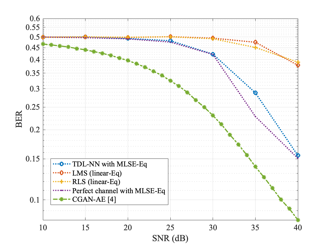
Figure 6: Performance comparison in terms of BER, 1- channel estimated from TDL-NN with MLSE equaliser, 2,3- linear equalizer with LMS and RLS algorithm for channel estimation, 4- perfect channel with MLSE equalizer, 5- CGAN channel model with AE to model Tx/Rx [4].

As discussed above, our TDL-NN model is a novel approach and is different from classical channel estimation. In order to compare our results with prior art, we calculate the BER (Bit Error Rate) after equalization and demodulation using the channel estimates provided by our TDL-NN model. Using BER, we can also compare our model with the CE methods, not necessarily estimating path delays and gains.

We used Matlab’s MLSE equalizer with our channel estimates to equalize the received signal, and BER is calculated for $90,000$ received signal samples for different SNR conditions for a scenario with 3 distinct multipaths. MLSE equalizer employs the Viterbi algorithm for decoding, which can also perform poorly in high noise conditions. In order to provide a fair comparison to TDL-NN, we also plot BER vs. SNR for a perfect channel using ray-tracing ground truth in Fig. 6. TDL-NN closely tracks MLSE equalization with the perfect channel and the errors in case of TDL-NN is largely due to MLSE equalization.

TDL-NN is also compared with Matlab’s linear equalizer using LMS (Lsast Mean Square) and RLS (Recursive Least Square) algorithms and performs very well compared to both as shown in the Fig. 6. However, we observe smaller BER with CGAN [4]. The approach in [4] models the end to end communication system with an autoencoder (transmitter with 5 and receiver with 8 hidden layers models) with CGAN (generator with 4 and discriminator with 6 hidden layers) modelling the channel effects and BER shows the overall performance, not just that of the CGAN. Moreover, the channel is trained using $5\times 10^{6}$ data samples with SNR = 35dB for all cases in [4] and the results are shown here after 32 iterations which took approximately 4 days on the same GPU, where TDL-NN is trained with $10,000$ data samples and $5,000$ training epochs in less than $1/2$ hour. We remark that for more complex channels with non-linear effects, GANs CE might be better than linear TDL-NN, but its computation time and training requirements make it unsuitable for practical scenarios. In contrast, our model can be refined for real-time applications. Moreover, TDL-NN estimates multipath delays and gains and provides visibility into the channel, which is especially useful for environment sensing and awareness.

IV-C Example Application: Drone Detection

In this section, we elaborate further on the interpretability of our TDL-NN model using a preliminary case study of detecting an authorised drone in an urban scenario. Our aim here is to show the potential of our TDL-NN approach, and detection of interesting events using estimated channel state is still work-in-progress. We created a scene using Matlab’s ray-tracing tool where four mobile users on an urban street are transmitting to four base-stations, mounted on the roofs, while a drone fly over the street at an height of 10m as shown in Fig. 7. The communication parameters are set as previous examples. During it’s flight, drone impacts some of the signal paths, which results in changes in channel state, both in delay and gains. For this preliminary example, we assume no traffic on the road. The objective is to detect the instances where a change happens. We used existing change/novelty detection algorithms for this purpose which can be trained on normal data and anomalies can be detected as outliers. For this experiment, we assume to have training data from the four base-stations without the interference of drone. The results of drone detection are presented in Table II. This is an on-going research project and we are building novel detection models based on the correlation between successively estimated channel states to detect sporadic events. Nevertheless, this example show the promising potential of our approach for environment awareness application.

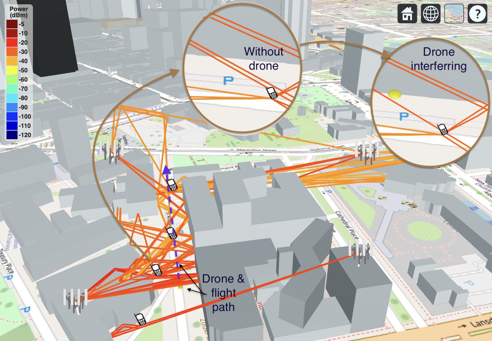
Figure 7: Scene with four mobile users transmitting each to a base-station, which are continuously monitoring channel states. A drone flying on the street impacts the signal multipaths as shown in insets.

TABLE II: Drone Detection Results

Model	Precision	Recall	F1 score
k-means	0.6667	0.5	0.5717
PCA with k-means	0.6667	0.6667	0.667
OCSVM	0.1667	0.6667	0.2667
LOF	0.2	1	0.3333
CBLOF	0.2143	1	0.3529
DeepSVDD	0.1875	1	0.3158

V Conclusion

In this paper, we present a practical low-complexity channel estimation approach based on a tapped delay line model. In our approach, the tap delays and gains are estimated through a neural network with one hidden layer. Our extensive experiments, using Matlab’s ray-tracing tool for generation of transmitted and received signal samples, show that this simple model can estimate the time-varying channel with reasonable accuracy in the presence of white noise and also in-band interference. This approach also enables developing a novel environmental awareness application where interesting objects and events can be detected through the changes in the channel state.

Although Matlab ray-tracing is an excellent resource for this research, we understand that our experiments are limited by how accurately ray-tracing is performed by the tool. The next step in this research is to apply the CE model in a real environment.

References

- [1] H. He, C.-K. Wen, S. Jin, and G. Y. Li, “Deep learning-based channel estimation for beamspace mmwave massive mimo systems,” IEEE Wireless Communications Letters, vol. 7, no. 5, pp. 852–855, 2018.
- [2] T. J. O’Shea, T. Roy, and N. West, “Approximating the void: Learning stochastic channel models from observation with variational generative adversarial networks,” in ICNC, pp. 681–686, 2019.
- [3] M. Soltani, V. Pourahmadi, A. Mirzaei, and H. Sheikhzadeh, “Deep learning-based channel estimation,” IEEE Communications Letters, vol. 23, no. 4, pp. 652–655, 2019.
- [4] H. Ye, L. Liang, G. Y. Li, and B.-H. Juang, “Deep learning-based end-to-end wireless communication systems with conditional gans as unknown channels,” IEEE TWC, vol. 19, no. 5, pp. 3133–3143, 2020.
- [5] A. Doshi and J. G. Andrews, “One-bit mmwave mimo channel estimation using deep generative networks,” IEEE Wireless Communications Letters, vol. 12, no. 9, pp. 1593–1597, 2023.
- [6] D. Luan and J. S. Thompson, “Channelformer: Attention based neural solution for wireless channel estimation and effective online training,” IEEE TWC, vol. 22, no. 10, pp. 6562–6577, 2023.
- [7] B. Böck, M. Baur, V. Rizzello, and W. Utschick, “Variational inference aided estimation of time varying channels,” in IEEE ICASSP, pp. 1–5, 2023.
- [8] B. Chatelier, L. L. Magoarou, and G. Redieteab, “Efficient Deep Unfolding for SISO-OFDM Channel Estimation,” in IEEE ICC, pp. 3475–3480, May 2023.
- [9] R. Hu, C. Hao, Y. Zhang, T. Yoo, J. Namgoong, and H. Xu, “Deep Learning-Based Channel Estimation with Low-Density Pilot in MIMO-OFDM Systems,” in IEEE ICC, pp. 2637–2642, May 2023.
- [10] A. K. Gizzini and M. Chafii, “Deep Learning Based Channel Estimation in High Mobility Communications Using Bi-RNN Networks,” in IEEE ICC, pp. 2625–2630, May 2023.
- [11] A. M. Jaradat, K. Walid Elgammal, M. K. Özdemir, and H. Arslan, “Identification of the number of wireless channel taps using deep neural networks,” in IEEE NEWCAS, pp. 1–4, 2021.
- [12] Z. Cheng, J. Huang, M. Tao, and P.-Y. Kam, “Swiss: Spectrum weighted identification of signal sources for mmwave systems,” in IEEE WCNC, pp. 1–6, 2018.
- [13] W. Kim, Y. Ahn, J. Kim, and B. Shim, “Towards deep learning-aided wireless channel estimation and channel state information feedback for 6G,” Journal of Comm. and Networks, vol. 25, no. 1, pp. 61–75, 2023.
- [14] A. Goldsmith, Wireless Communications. Cambridge University Press, 2005.
- [15] M. H. Hassoun, Fundamentals of Artificial Neural Networks. MIT Press, 1995.