Bayesian Federated Learning Via Expectation Maximization and Turbo Deep Approximate Message Passing

Abstract

Federated learning (FL) is a machine learning paradigm where the clients possess decentralized training data and the central server handles aggregation and scheduling. Typically, FL algorithms involve clients training their local models using stochastic gradient descent (SGD), which carries drawbacks such as slow convergence and being prone to getting stuck in suboptimal solutions. In this work, we propose a message passing based Bayesian federated learning (BFL) framework to avoid these drawbacks. Specifically, we formulate the problem of deep neural network (DNN) learning and compression and as a sparse Bayesian inference problem, in which group sparse prior is employed to achieve structured model compression. Then, we propose an efficient BFL algorithm called EM-TDAMP, where expectation maximization (EM) and turbo deep approximate message passing (TDAMP) are combined to achieve distributed learning and compression. The central server aggregates local posterior distributions to update global posterior distributions and update hyperparameters based on EM to accelerate convergence. The clients perform TDAMP to achieve efficient approximate message passing over DNN with joint prior distribution. We detail the application of EM-TDAMP to Boston housing price prediction and handwriting recognition, and present extensive numerical results to demonstrate the advantages of EM-TDAMP.

I Introduction

Federated learning (FL) [1] has become increasingly important in various artificial intelligence (AI) applications, including autonomous driving, healthcare and video analytics [2, 3, 4, 5]. In modern FL applications, deep neural network (DNN) is usually used, and local computation step is based on stochastic gradient descent (SGD) algorithms or its variations [6, 7]. To apply SGD to federated learning scenario, federated averaging (FedAvg) is commonly used as an aggregation mechanism to reduce communication rounds by increasing local iterations [8].

However, SGD-based FL algorithms have several limitations, including vanishing and exploding gradients [9, 10], the risk of getting stuck in suboptimal solutions [11], and slow convergence. Although there have been attempts to address these issues through advanced optimization techniques like Adam [7], the overall convergence remains slow for high training accuracy requirements, which limits the application scenarios of SGD-based FL.

AI applications often require DNN models with a large number of parameters, posing challenges for training and inference. To mitigate the computational load in DNN inference, researchers have proposed several model compression techniques. Traditional regularization methods generate networks with random sparse connectivity, requiring high-dimensional matrices. Group sparse regularization has been introduced to eliminate redundant neurons, features, and filters [12, 13, 14]. Recent work has addressed neuron-wise, feature-wise, and filter-wise groupings within a single sparse regularization term [15]. However, for regularization-based pruning methods, it is difficult to achieve the exact compression ratio after training. Thus, there is a need for a new learning and compression framework that enhances convergence beyond SGD.

Another drawback of traditional DNN models is their tendency to be overconfident in their predictions, which can be problematic in applications such as autonomous driving and medical diagnostics [16, 17, 18], where silent failure can lead to dramatic outcomes. To overcome this problem, Bayesian deep learning has been proposed, allowing for uncertainty quantification [19]. Bayesian deep learning formulates DNN training as a Bayesian inference problem, where the DNN parameters with a prior distribution serve as hypotheses, and the training set $\boldsymbol{D}$ consists of features $\boldsymbol{D}_{x}$ and labels $\boldsymbol{D}_{y}$. Calculating the exact Bayesian posterior distribution $p\left(\boldsymbol{\theta}|\boldsymbol{D}\right)$ for a DNN is extremely challenging, and a widely used method is variational Bayesian inference (VBI), where a variational distribution $q_{\varphi}\left(\boldsymbol{\theta}\right)$ with parameters $\varphi$ is proposed to approximate the exact posterior $p\left(\boldsymbol{\theta}|\boldsymbol{D}\right)$ [20, 21]. However, most VBI algorithms still rely on SGD for optimizing variational distribution parameters $\varphi$, where loss function is often defined as the Kullback-Leibler divergence between $q_{\varphi}\left(\boldsymbol{\theta}\right)$ and $p\left(\boldsymbol{\theta}|\boldsymbol{D}\right)$ [22, 20, 21], leading to common drawbacks of SGD-based training algorithms.

In this paper, we propose a novel Bayesian federated learning framework for distributed learning and compression of DNN with superior convergence speed and learning performance. The main contributions are summarized as follows.

• Bayesian federated learning framework with structured model compression: We propose a Bayesian federated learning framework to enable learning and structured compression for DNN. Firstly, we formulate the DNN learning problem as Bayesian inference of the DNN parameters. Then we propose a group sparse prior distribution to achieve efficient neuron-level pruning during training. We further incorporate zero-mean Gaussian noise in the likelihood function to control the learning rate through noise variance. To accelerate convergence, we update hyperparameters in the prior distribution and the likelihood function based on expectation maximization (EM) algorithm. In addition, we separate the algorithm into central server part and clients part to apply the Bayesian framework in federated learning scenarios. The clients utilize turbo deep approximate message passing (TDAMP) for local training. The central server computes the global posterior distribution based on an efficient aggregation method, and then update hyperparameters based on EM algorithm, which will be broadcast to clients in the next round.

• Turbo deep approximate message passing algorithm: To facilitate local training at clients, we propose a TDAMP algorithm. Due to the existence of many loops in the DNN factor graph and the high computational complexity, we cannot directly apply the standard sum-product rule. Although various approximate message passing methods have been proposed to reduce the complexity of message passing for linear and bi-linear models in the compressed sensing literature [23, 24, 25], to the best of our knowledge, there is no efficient message passing algorithm available for training the DNN with both multiple layers and structured sparse parameters. TDAMP iterates between two Modules: Module $B$ performs message passing over the group sparse prior distribution, and Module $A$ performs deep approximate message passing (DAMP) over the DNN using independent prior distribution from Module $B$. The proposed TDAMP overcomes the aforementioned drawbacks of SGD-based training algorithms, showing faster convergence and superior inference performance in simulations.

• Specific EM-TDAMP algorithm design for two applications: We apply EM-TDAMP to Boston housing price prediction and handwriting recognition [26], and present extensive numerical results to verify the advantages of EM-TDAMP. Extensive numerical results demonstrate that EM-TDAMP achieves faster convergence (and thus lower communication overhead for FL) and better prediction/recognition performance compared to SGD-based training algorithms.

The rest of the paper is organized as follows. Section II presents the problem formulation for Bayesian federated learning with structured model compression. Section III derives the EM-TDAMP algorithm and discusses various implementation issues. Section IV details the application of DAMP to Boston housing price prediction and handwriting recognition. Finally, the conclusion is given in Section VI.

II Bayesian Federated Learning Framework

II-A DNN Model and Standard Training Procedure

A general DNN consists of one input layer, multiple hidden layers and one output layer. In this paper, we focus on feedforward DNNs for easy illustration. Let $\boldsymbol{z}_{L}=\phi\left(\boldsymbol{u}_{0};\boldsymbol{\theta}\right)$ be a DNN with $L$ layers that maps the input vector $\boldsymbol{u}_{0}=\boldsymbol{x}\in\mathbb{R}^{N_{0}}$ to the output vector $\boldsymbol{z}_{L}\in\mathbb{R}^{N_{L}}$ with a set of parameters $\boldsymbol{\theta}$. The input and output of each layer, denoted as $\boldsymbol{u}_{l-1}\in\mathbb{R}^{N_{l-1}}$ and $\boldsymbol{z}_{l}\in\mathbb{R}^{N_{l}}$ respectively, can be expressed as follows:

$$\boldsymbol{z}_{l}=\boldsymbol{W}_{l}\boldsymbol{u}_{l-1}+\boldsymbol{b}_{l},l=1,\ldots,L,$$

$$\boldsymbol{u}_{l}=\zeta_{l}\left(\boldsymbol{z}_{l}\right),l=1,\ldots,L-1,$$

where $\boldsymbol{W}_{l}\in\mathbb{R}^{N_{l}\times N_{l-1}}$, $\boldsymbol{b}_{l}\in\mathbb{R}^{N_{l}}$ and $\zeta_{l}\left(\cdot\right)$ account for the weight matrix, the bias vector and the activation function in layer $l$, respectively. As is widely used, we set $\zeta_{l}\left(\cdot\right)$ as rectified linear units (ReLU) defined as:

$$\zeta_{l}\left(z\right)=\begin{cases}z&z>0\\ 0&z\leq 0\end{cases}.$$ (1)

For classification model, the output $\boldsymbol{z}_{L}$ is converted into a predicted class $u_{L}$ from the set of possible labels/classes $\left\{1,\ldots,N_{L}\right\}$ using the argmax layer:

$$u_{L}=\zeta_{L}\left(\boldsymbol{z}_{L}\right)=\mathop{\arg\max}\limits_{m}z_{L,m},$$ (2)

where $z_{L,m}$ represents the output related to the $m$-th label. However, the derivative of argmax activation function is discontinuous, which may lead to numerical instability. As a result, it is usually replaced with softmax when using SGD-based algorithms to train the DNN. In the proposed framework, to facilitate message passing algorithm design, we add zero-mean Gaussian noise on $\boldsymbol{z}_{L}$, which will be further discussed in Subsection II-B2.

The set of parameters $\boldsymbol{\theta}$ is defined as $\boldsymbol{\theta}\triangleq\left\{\boldsymbol{W}_{l},\boldsymbol{b}_{l}|l=1,\ldots,L\right\}$. In practice, the DNN parameters $\boldsymbol{\theta}$ are usually obtained through a deep learning/training algorithm, which is the process of regressing the parameters $\boldsymbol{\theta}$ on some training data $\boldsymbol{D}\triangleq\left\{\left(\boldsymbol{x}^{i},\boldsymbol{y}^{i}\right)|i=1,\ldots,I\right\}$, usually a series of inputs $\boldsymbol{D}_{x}\triangleq\left\{\boldsymbol{x}^{i}|i=1,\ldots,I\right\}$ and their corresponding labels $\boldsymbol{D}_{y}\triangleq\left\{\boldsymbol{y}^{i}|i=1,\ldots,I\right\}$. The standard approach is to minimize a loss function $L\left(\boldsymbol{\theta}\right)$ to find a point estimate of $\boldsymbol{\theta}$ using the SGD-based algorithms. The loss function is often defined as the log likelihood of the training set, e.g., $L\left(\boldsymbol{\theta}\right)\triangleq\frac{1}{v}\sum_{i=1}^{I}\left\|\boldsymbol{y}^{i}-\phi\left(\boldsymbol{x}^{i};\boldsymbol{\theta}\right)\right\|^{2}$, where $v$ reflects the confidence in the predictive power of the model $\phi\left(\boldsymbol{x};\boldsymbol{\theta}\right)$. Sometimes, a regularization term is added to the loss function to penalize or compress the DNN model, e.g., $L\left(\boldsymbol{\theta}\right)\triangleq\frac{1}{v}\sum_{i=1}^{I}\left\|\boldsymbol{y}^{i}-\phi\left(\boldsymbol{x}^{i};\boldsymbol{\theta}\right)\right\|^{2}+\lambda\left\|\boldsymbol{\theta}\right\|_{1}$, where $\lambda$ controls the degree of regularization when using the $l_{1}$-norm regularization function to prune the DNN parameters. It is also possible to use more complicated sparse regularization functions to remove redundant neurons, features and filters [12, 13, 14]. However, the above standard training procedure has several drawbacks as discussed in the introduction. Therefore, in this paper, we propose a Bayesian learning formulation to overcome those drawbacks.

II-B Bayesian Federated Learning Framework with Structured Model Compression

In the proposed Bayesian federated learning (BFL) framework, the parameters $\boldsymbol{\theta}$ are treated as random variables. The goal of the proposed framework is to obtain the Bayesian posterior distribution $p\left(\boldsymbol{\theta}|\boldsymbol{D}\right)$, which can be used to predict the output distribution (i.e., both point estimation and uncertainty for the output) on test data through forward propagation similar to that in training process. The joint posterior distribution $p\left(\boldsymbol{\theta},\boldsymbol{z}_{L}|\boldsymbol{D}\right)$ can be factorized as (3):

$$p\left(\boldsymbol{\theta},\boldsymbol{z}_{L}|\boldsymbol{D}\right) \propto p\left(\boldsymbol{\theta},\boldsymbol{z}_{L},\boldsymbol{D}_{y}|\boldsymbol{D}_{x}\right)$$

$$=p\left(\boldsymbol{\theta}\right)p\left(\boldsymbol{z}_{L}|\boldsymbol{D}_{x},\boldsymbol{\theta}\right)p\left(\boldsymbol{D}_{y}|\boldsymbol{z}_{L}\right).$$ (3)

The prior distribution $p\left(\boldsymbol{\theta}\right)$ is set as group sparse to achieve model compression/dropout as will be detailed in Subsection II-B1. The likelihood function $p\left(\boldsymbol{D}_{y}|\boldsymbol{z}_{L}\right)$ is chosen as Gaussian/Probit-product to prevent numerical instability, as will be detailed in Subsection II-B2.

II-B1 Group Sparse Prior Distribution for DNN Parameters

Different applications often have varying requirements regarding the structure of DNN parameters. In the following, we shall introduce a group sparse prior distribution to capture structured sparsity that may arise in practical scenarios. Specifically, the joint prior distribution $p\left(\boldsymbol{\theta}\right)$ is given by

$$p\left(\boldsymbol{\theta}\right) =\prod_{i=1}^{Q}\left(\rho_{i}\prod_{j\in\mathcal{N}_{i}}g_{j}\left(\theta_{j}\right)+\left(1-\rho_{i}\right)\prod_{j\in\mathcal{N}_{i}}\delta\left(\theta_{j}\right)\right),$$ (4)

where $Q$ represents the number of groups, $\rho_{i}$ represents the active probability for the $i$-th group, $\mathcal{N}_{i}$ represents the set consisting of indexes of $\theta$ in the $i$-th group and $g_{j}\left(\theta_{j}\right)$ represents the probability density function (PDF) of $\theta_{j},j\in\mathcal{N}_{i}$ when active, which is chosen as a Gaussian distribution with expectation $\mu_{j}$ and variance $v_{j}$ denoted as $N\left(\theta_{j};\mu_{j},v_{j}\right)$ in this paper. For convenience, we define a set $\boldsymbol{\psi}$ consisting hyperparameters $\rho_{i}$, $\mu_{j}$ and $v_{j}$ for $i=1,\ldots,Q,j\in\mathcal{N}_{i}$, which will be updated to accelerate convergence as will be further discussed later. Here we shall focus on the following group sparse prior distribution to enable structured model compression.

Independent Sparse Prior for Bias Pruning

To impose simple sparse structure on the bias parameters for random dropout, we assume the elements $b_{m},m=1,\ldots,Q_{b}\triangleq\sum_{l=1}^{L}N_{l}$ have independent prior distributions:

$$p\left(\boldsymbol{b}\right) =\prod_{m=1}^{Q_{b}}p\left(b_{m}\right),$$

where

$$p\left(b_{m}\right)=\rho_{m}^{b}N\left(b_{m};\mu_{m}^{b},v_{m}^{b}\right)+\left(1-\rho_{m}^{b}\right)\delta\left(b_{m}\right),$$

$\rho_{m}^{b}$ represents the active probability, and $\mu_{m}^{b}$ and $v_{m}^{b}$ represent the expectation and variance when active.

Group Sparse Prior for Neuron Pruning

In most DNNs, a weight group is often defined as the outgoing weights of a neuron to promote neuron-level sparsity. Note that there are a total number of $\sum_{l=1}^{L}N_{l-1}$ input neurons and hidden neurons in the DNN. In order to force all outgoing connections from a single neuron (corresponding to a group) to be either simultaneously zero or not, we divide the weight parameters into $Q_{W}\triangleq\sum_{l=1}^{L}N_{l-1}$ groups, such that the $i$-th group for $i=1,\ldots,Q_{W}$ corresponds to the weights associated with the $i$-th neuron. Specifically, for the $i$-th weight group $\boldsymbol{W}_{i}$, we denote the active probability as $\rho_{i}^{W}$, and the expectation and variance related to the $n$-th element $W_{i,n},n\in\mathcal{N}_{i}^{W}$ as $\mu_{i,n}^{W}$ and $v_{i,n}^{W}$. The joint prior distribution can be decomposed as:

$$p\left(\boldsymbol{W}\right) =\prod_{i=1}^{Q_{W}}p\left(\boldsymbol{W}_{i}\right),$$

where

$$p\left(\boldsymbol{W}_{i}\right) =\rho_{i}^{W}\prod_{n\in\mathcal{N}_{i}^{W}}N\left(W_{i,n};\mu_{i,n}^{W},v_{i,n}^{W}\right)$$

$$+\left(1-\rho_{i}^{W}\right)\prod_{n\in\mathcal{N}_{i}^{W}}\delta\left(W_{i,n}\right),$$

Note that a parameter $\theta_{j}$ corresponds to either a bias parameter $b_{m}$ or a weight parameter $W_{i,n}$, and thus we have $Q=Q_{b}+Q_{W}$. For convenience, we define $\boldsymbol{\psi}$ as a set consisting of $\rho_{m}^{b},\mu_{m}^{b},v_{m}^{b}$ for $m=1,\cdots,Q_{b}$ and $\rho_{i}^{W},\mu_{i,n}^{W},v_{i,n}^{W}$ for $i=1,\cdots,Q_{W},n\in\mathcal{N}_{i}$. Please refer to Fig. 1 for an illustration of group sparsity. It is also possible to design other sparse priors to achieve more structured model compression, such as burst sparse prior to concentrate the active neurons in each layer on a few clusters. The details are omitted due to limited space.

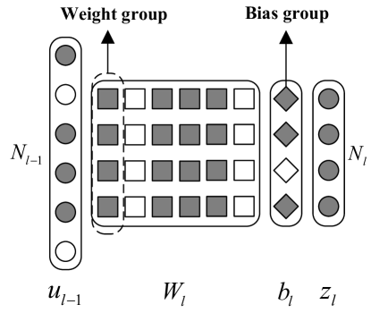
Figure 1: Illustration for group sparse prior.

II-B2 Likelihood Function for the Last Layer

In Bayesian inference problem, the observation can be represented as a likelihood function $p\left(\boldsymbol{y}^{i}|\boldsymbol{z}_{L}^{i}\right)$ for $i=1,\ldots,I$, where we define $\boldsymbol{z}_{L}^{i}=\phi\left(\boldsymbol{x}^{i};\boldsymbol{\theta}\right)$. Directly assume $p\left(\boldsymbol{y}^{i}|\boldsymbol{z}_{L}^{i}\right)=\delta\left(\boldsymbol{y}^{i}-\zeta_{L}\left(\boldsymbol{z}_{L}^{i}\right)\right)$ may lead to numerical instability. To avoid this problem, we add zero-mean Gaussian noise with variance $v$ on the output $\boldsymbol{z}_{L}^{i}$. The noise variance $v$ is treated as a hyperparameter that is adaptively updated to control the learning rate. In the following, we take regression model and classification model as examples to illustrate the modified likelihood function.

Gaussian Likelihood Function for Regression Model

For regression model, after adding Gaussian noise at output, the likelihood function becomes joint Gaussian:

$$p\left(\boldsymbol{y}^{i}|\boldsymbol{z}_{L}^{i}\right) =\prod_{m=1}^{N_{L}}N\left(y_{m}^{i};\boldsymbol{z}_{L,mi},v\right),$$ (5)

where $v,y_{m}^{i}$ and $\boldsymbol{z}_{L,mi}$ represent the noise variance, the $m$-th element in $\boldsymbol{y}^{i}$ and $\boldsymbol{z}_{L}^{i}$, respectively.

Probit-product Likelihood Function for Classification Model

For classification model, we consider one-hot label, where $y^{i}$ refers to the label for the $i$-th training sample. Instead of directly using argmax layer [27], to prevent message vanishing and booming, we add Gaussian noise on $z_{L,mi}$ for $m=1,\ldots,N_{L}$ and obtain the following likelihood function which is product of probit function mentioned in [28]:

$$p\left(y^{i}|\boldsymbol{z}_{L}^{i}\right) \approx\sum_{u_{L}^{i}=1}^{N_{L}}\delta\left(y^{i}-u_{L}^{i}\right)\prod_{m\neq u_{L}^{i}}p\left(z_{L,mi}<z_{L,u_{L}^{i}i}\right)$$

$$=\prod_{m\neq y^{i}}Q\left(\frac{z_{L,mi}-z_{L,y^{i}i}}{\sqrt{v}}\right),$$ (6)

where we approximate $z_{L,mi}-z_{L,u_{L}^{i}i},i=1,\ldots,I,m\neq u_{L}^{i}$ as independent to simplify the message passing as will be detailed in Appendix -A2. Extensive simulations verify that such an approximation can achieve a good classification performance. Besides, we define $Q\left(\cdot\right)=1-F\left(\cdot\right)$, where $F\left(\cdot\right)$ represents the cumulative distribution function of the standardized normal random variable.

II-B3 Outline of Bayesian Federated Learning Algorithm

To accelerate convergence, we update hyperparameters in the prior distribution and the likelihood function based on expectation maximization (EM) algorithm [29], where the expectation step (E-step) computes the posterior distribution (3), while the maximization step (M-step) update hyperparameters. The two steps execute alternately until convergence.

Furthermore, we consider a general federated/distributed learning scenario, which includes centralized learning as a special case. There is a central server and $K$ clients, where each client $k=1,\ldots,K$ possesses a subset of data (local data sets) indexed by $\mathcal{I}_{k}$: $\boldsymbol{D}^{k}\triangleq\left\{\boldsymbol{D}_{x}^{k},\boldsymbol{D}_{y}^{k}\right\}$ with $\boldsymbol{D}_{x}^{k}\triangleq\left\{\boldsymbol{x}^{i}|i\in\mathcal{I}_{k}\right\}$, $\boldsymbol{D}_{y}^{k}\triangleq\left\{\boldsymbol{y}^{i}|i\in\mathcal{I}_{k}\right\}$ and $\cup_{k=1}^{K}\mathcal{I}_{k}=\left\{1,2,\ldots,I\right\}$. The process of the proposed BFL contains three steps as illustrated in Fig. 2. Firstly, the central server sends the prior hyperparameters $\boldsymbol{\psi}$ and the likelihood hyperparameter $v$ (i.e., noise variance) to clients to initialize local prior distribution $p\left(\boldsymbol{\theta}\right)$ and likelihood function $p\left(\boldsymbol{D}_{y}^{k}|\boldsymbol{z}_{L}^{k}\right)$, where $\boldsymbol{z}_{L}^{k}$ represents the output corresponding to the local data $\boldsymbol{D}_{x}^{k}$. Afterwards, the clients parallelly compute local posterior parameters $\boldsymbol{\varphi}^{k}$ and $\sigma^{k}$ by performing turbo deep approximate message passing (TDAMP) as will be detailed in Subsection III-B. Lastly, the central server aggregates local posterior parameters to update hyperparameters $\boldsymbol{\psi}$ and $v$ by maximizing the following expectation:

$$\left\{\boldsymbol{\psi},v\right\} =\mathop{\arg\max}\limits_{\boldsymbol{\psi},v}E\left(\log p\left(\boldsymbol{\theta},\boldsymbol{z}_{L},\boldsymbol{D}\right)\right)$$

$$=\mathop{\arg\max}\limits_{\boldsymbol{\psi}}E\left(\log p\left(\boldsymbol{\theta}\right)\right)$$

$$+\mathop{\arg\max}\limits_{v}E\left(\log p\left(\boldsymbol{D}_{y}|\boldsymbol{z}_{L}\right)\right),$$ (7)

where the expectation is taken w.r.t. the posterior distributions $p\left(\boldsymbol{\theta}|\boldsymbol{D}\right)$ and $p\left(\boldsymbol{z}_{L}|\boldsymbol{D}\right)$, and $\boldsymbol{\psi},v$ can be approximated as function of $\boldsymbol{\varphi}^{k},\sigma^{k},k=1,\ldots,K$ as will be detailed in Subsection III-A. The definitions of the local posterior parameters $\boldsymbol{\varphi}^{k},\sigma^{k}$, the updating rules at the central server and the TDAMP algorithm at the clients will be elaborated in the next section.

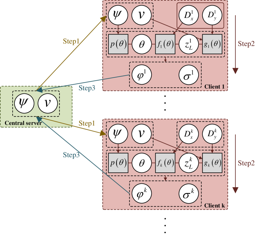
Figure 2: Illustration for federated learning framework, where $f_{k}\left(\boldsymbol{\theta}\right),g_{k}\left(\boldsymbol{\theta}\right)$ represents $p\left(\boldsymbol{z}_{L}^{k}|\boldsymbol{D}_{x}^{k},\boldsymbol{\theta}\right)$ and $p\left(\boldsymbol{D}_{y}^{k}|\boldsymbol{z}_{L}^{k}\right)$, respectively for $k=1,\ldots,K$.

III Algorithm Derivation

III-A Updating Rules At the Central Server

The central server computes the global posterior distribution by aggregating the local posterior distributions in the E-step, and update the hyperparameters by maximizing the objective function (7) in the M-step. In the following, we derive the specific updating rules.

III-A1 E-step

To compute the expectation in (7), the E-step calculates the global posterior distribution $p\left(\boldsymbol{\theta}|\boldsymbol{D}\right)$ and $p\left(\boldsymbol{z}_{L}|\boldsymbol{D}\right)$.

Global posterior distribution for $\boldsymbol{\theta}$

We approximate $p\left(\boldsymbol{\theta}|\boldsymbol{D}\right)$ as the weighted geometric average of local posterior distributions $p\left(\boldsymbol{\theta}|\boldsymbol{D}^{k}\right),k=1,\ldots,K$ [30]:

$$p\left(\boldsymbol{\theta}|\boldsymbol{D}\right)\approx\prod_{k=1}^{K}\left(p\left(\boldsymbol{\theta}|\boldsymbol{D}^{k}\right)\right)^{\frac{I_{k}}{I}},$$ (8)

where $I_{k}=\left|\mathcal{I}_{k}\right|$. The proposed weighted geometric average of $p\left(\boldsymbol{\theta}|\boldsymbol{D}^{k}\right),k=1,\ldots,K$ in (8) is more likely to approach the global optimal posterior distribution compared to widely used weighted algebraic average. Here we give an intuitive illustration through a special case. Assuming $I_{k}=\frac{I}{K}$ for $k=1,\ldots,K$, and all the local posterior distributions are Gaussian (note that Gaussian is a special case of the Bernoulli-Gaussian). The posterior distribution based on (8) is still Gaussian, whose expectation is the average of local posterior expectations weighted by the corresponding variances. This approximation is more reliable because it utilizes the local variances for expectation aggregation, and it is consistent with the experiment results [30].

Next, we give the specific expression for global posterior distribution $p\left(\boldsymbol{\theta}|\boldsymbol{D}\right)$ in (8). As will be detailed in Subsection III-B, $p\left(\boldsymbol{\theta}|\boldsymbol{D}^{k}\right)$ is approximated as the product of marginal posterior distributions (which has been widely used in the literature since the marginal posterior distributions can be efficiently computed using the factor graph and message passing approach):

$$p\left(\boldsymbol{\theta}|\boldsymbol{D}^{k}\right) \approx\prod_{m=1}^{Q_{b}}p\left(b_{m}|\boldsymbol{D}^{k}\right)\prod_{i=1}^{Q_{W}}p\left(\boldsymbol{W}_{n\in\mathcal{N}_{i}}|\boldsymbol{D}^{k}\right),$$

where the marginal posterior distributions are group Bernoulli-Gaussian denoted as follows:

$$p\left(b_{m}|\boldsymbol{D}^{k}\right)=\rho_{b_{m},k}N\left(b_{m};\mu_{b_{m},k},v_{b_{m},k}\right)+\left(1-\rho_{b_{m},k}\right)\delta\left(b_{m}\right),$$

$$p\left(\boldsymbol{W}_{n\in\mathcal{N}_{i}}|\boldsymbol{D}^{k}\right) =\rho_{W_{i},k}\prod_{n\in\mathcal{N}_{i}}N\left(W_{i,n};\mu_{W_{i,n},k},v_{W_{i,n},k}\right)$$

$$+\left(1-\rho_{W_{i},k}\right)\prod_{n\in\mathcal{N}_{i}}\delta\left(W_{i,n}\right).$$

For convenience, we denote the local posterior parameters $\boldsymbol{\varphi}^{k}$ as a set consisting of $\rho_{b_{m},k},\mu_{b_{m},k},v_{b_{m},k}$ for $m=1,\cdots,Q_{b}$ and $\rho_{W_{i},k},\mu_{W_{i,n},k},v_{W_{i,n},k}$ for $i=1,\cdots,Q_{W},n\in\mathcal{N}_{i}$, which are sent to the central server in uplink communication. Notice that when the local posterior distributions are products of group Bernoulli-Gaussian, it is difficult to derive the exact expression for the global posterior distribution based on (8). Thus, we approximate the global posterior distribution as product of group Bernoulli-Gaussian (9)-(11).

$$q\left(\boldsymbol{\theta}\right) =\prod_{m=1}^{Q_{b}}q_{b_{m}}\left(b_{m}\right)\prod_{i=1}^{Q_{W}}q_{W_{i}}\left(\boldsymbol{W}_{n\in\mathcal{N}_{i}}\right),$$ (9)

$$q_{b_{m}}\left(b_{m}\right)=\rho_{b_{m}}N\left(b_{m};\mu_{b_{m}},v_{b_{m}}\right)+\left(1-\rho_{b_{m}}\right)\delta\left(b_{m}\right),$$ (10)

$$q_{W_{i}}\left(\boldsymbol{W}_{n\in\mathcal{N}_{i}}\right) =\rho_{W_{i}}\prod_{n\in\mathcal{N}_{i}}N\left(W_{i,n};\mu_{W_{i,n}},v_{W_{i,n}}\right)$$

$$+\left(1-\rho_{W_{i}}\right)\prod_{n\in\mathcal{N}_{i}}\delta\left(W_{i,n}\right),$$ (11)

where the parameters are chosen by minimizing the Kullback-Leibler divergence $D_{KL}\left(p\left(\boldsymbol{\theta}|\boldsymbol{D}\right)||q\left(\boldsymbol{\theta}\right)\right)$, and $p\left(\boldsymbol{\theta}|\boldsymbol{D}\right)$ is given in (8). The detailed derivation is omitted, and we directly present the updating rules:

$$\mu_{b_{m}}=\frac{\sum_{k=1}^{K}\frac{I_{k}\mu_{b_{m},k}}{Iv_{b_{m},k}}}{\sum_{k=1}^{K}\frac{I_{k}}{Iv_{b_{m},k}}},v_{b_{m}}=\frac{1}{\sum_{k=1}^{K}\frac{I_{k}}{Iv_{b_{m},k}}},$$ (12)

$$\rho_{b_{m}}=\frac{1}{1+\frac{1}{C_{b_{m}}}\prod_{k=1}^{K}\left(\frac{1-\rho_{b_{m},k}}{\rho_{b_{m},k}}\right)^{\frac{I_{k}}{I}}},$$ (13)

$$\mu_{W_{i,n}}=\frac{1}{\sum_{k=1}^{K}\frac{I_{k}}{Iv_{W_{i,n},k}}},v_{W_{i,n}}=\frac{\sum_{k=1}^{K}\frac{I_{k}\mu_{W_{i,n},k}}{Iv_{W_{i,n},k}}}{\sum_{k=1}^{K}\frac{I_{k}}{Iv_{W_{i,n},k}}},$$ (14)

$$\rho_{W_{i}}=\frac{1}{1+\frac{1}{C_{W_{i}}}\prod_{k=1}^{K}\left(\frac{1-\rho_{W_{i},k}}{\rho_{W_{i},k}}\right)^{\frac{I_{k}}{I}}},$$ (15)

where

$$C_{b_{m}}=\frac{\prod_{k=1}^{K}\left(N\left(\mu_{b_{m},k},v_{b_{m},k}\right)\right)^{\frac{I_{k}}{I}}}{N\left(\mu_{b_{m}},v_{b_{m}}\right)},$$

$$C_{W_{i}}=\prod_{n\in\mathcal{N}_{i}}\left(\frac{\prod_{k=1}^{K}\left(N\left(\mu_{W_{i,n},k},v_{W_{i,n},k}\right)\right)^{\frac{I_{k}}{I}}}{N\left(\mu_{W_{i,n}},v_{W_{i,n}}\right)}\right).$$

Global posterior distribution for $\boldsymbol{z}_{L}$

We assume $\boldsymbol{z}_{L}^{k},k=1,\ldots,K$ are independent and approximate $p\left(\boldsymbol{z}_{L}|\boldsymbol{D}\right)$ as

$$p\left(\boldsymbol{z}_{L}|\boldsymbol{D}\right)=\prod_{k=1}^{K}p\left(\boldsymbol{z}_{L}^{k}|\boldsymbol{D}^{k}\right),$$ (16)

which is reasonable since $\boldsymbol{z}_{L}^{k}$ is mainly determined by the $k$-th local data set $\boldsymbol{D}^{k}$ that is independent of the other local data sets $\boldsymbol{D}^{k^{{}^{\prime}}},k^{{}^{\prime}}\neq k$.

Similarly, the local posterior distribution $p\left(\boldsymbol{z}_{L}^{k}|\boldsymbol{D}^{k}\right)$ is also approximated as the product of Gaussian marginal posterior distributions (17) as will be discussed in Subsection III-B:

$$p\left(\boldsymbol{z}_{L}^{k}|\boldsymbol{D}^{k}\right) \approx\prod_{i\in\mathcal{I}_{k}}\prod_{m=1}^{N_{L}}N\left(z_{L,mi};\mu_{z_{L,mi}},v_{z_{L,mi}}\right).$$ (17)

where $\boldsymbol{z}_{L}^{k}=\left\{\boldsymbol{z}_{L,mi}|m=1,\ldots,N_{L},i\in\mathcal{I}_{k}\right\}\in\mathbb{R}^{N_{L}\times I_{k}}$ and $p\left(\boldsymbol{z}_{L}^{k}|\boldsymbol{D}^{k}\right)$ represent the output at client $k$ and the related posterior distribution, respectively. By plugging (17) into (16), we achieve the global posterior distribution for $\boldsymbol{z}_{L}$.

III-A2 M-step

In the M-step, we update hyperparameters $\boldsymbol{\psi}$ and $v$ in the prior distribution and the likelihood function by maximizing $E\left(\log p\left(\boldsymbol{\theta}\right)\right)$ and $E\left(\log p\left(\boldsymbol{D}_{y}|\boldsymbol{z}_{L}\right)\right)$ respectively, where the expectation is computed based on the results of the E-step as discussed above.

Updating rules for prior hyperparameter $\boldsymbol{\psi}$

We observe that the approximated posterior distribution $q\left(\boldsymbol{\theta}\right)$ (9) and the prior distribution $p\left(\boldsymbol{\theta}\right)$ (4) can be factorized in the same form, thus maximizing $E\left(\log p\left(\boldsymbol{\theta}\right)\right)$ is equivalent to update $p\left(\boldsymbol{\theta}\right)$ as $q\left(\boldsymbol{\theta}\right)$. In other words, we update $\boldsymbol{\psi}$ as the corresponding parameters in $q\left(\boldsymbol{\theta}\right)$ as given in (12)-(15). However, directly updating the prior sparsity parameters $\rho_{i}^{W}$s based on EM cannot achieve neuron-level pruning with the target sparsity $\rho$. It is also not a good practice to fix $\rho_{i}^{W}=\rho$ throughout the iterations because this usually slows down the convergence speed as observed in the simulations. In order to control the network sparsity and prune the network during training without affecting the convergence, we introduce the following modified updating rules for $\rho_{i}^{W}$s. Specifically, after each M-step, we calculate $S$, which represents the number of weight groups that are highly likely to be active, i.e.,

$$S=\sum_{i=1}^{Q_{W}}1\left(\rho_{i}^{W}>\rho_{th}\right),$$

where $\rho_{th}$ is certain threshold that is set close to 1. If $S$ exceeds the target number of groups $\rho Q$, we reset $\rho_{i}^{W}$s as follows:

$$\rho_{i}^{W}=\begin{cases}\rho_{0},&\rho_{i}^{W}\geq\rho_{th}\\ 0,&\rho_{i}^{W}<\rho_{th}\end{cases},$$

where $\rho_{0}$ is the initial sparsity. Extensive simulations have shown that this method works well.

Updating rules for noise variance $v$

In federated learning, based on (16), the expectation $E\left(\log p\left(\boldsymbol{D}_{y}|\boldsymbol{z}_{L}\right)\right)$ can be written as:

$$E\left(\log p\left(\boldsymbol{D}_{y}|\boldsymbol{z}_{L}\right)\right) =\sum_{k=1}^{K}E\left(\log p\left(\boldsymbol{D}_{y}^{k}|\boldsymbol{z}_{L}^{k}\right)\right),$$

where the expectation is w.r.t. (16), which can be computed based on local posterior distributions (17). In practice, for $E\left(\log p\left(\boldsymbol{D}_{y}|\boldsymbol{z}_{L}\right)\right)$, the maximum point w.r.t. $v$ can be expressed as a function of local posterior parameters. This means that the clients only need to send a few posterior parameters denoted as $\sigma^{k},k=1,\ldots,K$ instead of the posterior distributions $p\left(\boldsymbol{z}_{L}^{k}|\boldsymbol{D}^{k}\right),k=1,\ldots,K$ to the central server. In the following, we take regression model and classification model as examples to derive the updating rule for $v$ and define parameters $\sigma^{k}$ at client $k$ to compress parameters in uplink communication.

For regression model (5), by setting the derivative for $E\left(\log p\left(\boldsymbol{D}_{y}|\boldsymbol{z}_{L}\right)\right)$ w.r.t. $v$ equal to zero, we obtain:

$$v^{*}=\sum_{k=1}^{K}\frac{I_{k}}{I}\sigma_{k},$$ (18)

where

$$\sigma_{k}\triangleq\sum_{i\in\mathcal{I}_{k}}\sum_{m=1}^{N_{L}}\frac{\left(y_{m}^{i}-\mu_{z_{L,mi}}\right)^{2}+v_{z_{L,mi}}}{N_{L}I^{k}}.$$ (19)

For classification model (6), for $i=1,\ldots,I,m\neq y^{i}$, we define:

$$\xi_{mi}=z_{L,mi}-z_{L,y^{i}i},$$

with expectation and variance given by

$$\mu_{\xi_{mi}}=\mu_{z_{L,mi}}-\mu_{z_{L,y^{i}i}}, v_{\xi_{mi}}=v_{z_{L,mi}}+v_{z_{L,y^{i}i}}.$$ (20)

Then $E\left(\log p\left(\boldsymbol{D}_{y}|\boldsymbol{z}_{L}\right)\right)$ can be approximated as follows:

$$E\left(\log p\left(\boldsymbol{D}_{y}|\boldsymbol{z}_{L}\right)\right)= \int_{\xi_{mi}}\log Q\left(\frac{\xi_{mi}}{\sqrt{v}}\right)$$

$$\times\sum_{i=1}^{I}\sum_{m\neq y^{i}}N\left(\xi_{mi};\mu_{\xi_{mi}},v_{\xi_{mi}}\right)$$

$$\approx \int_{\xi}G\left(\xi;\alpha_{\xi},\beta_{\xi}\right)\log Q\left(\frac{\xi}{\sqrt{v}}\right),$$ (21)

where we approximate $\xi\sim\sum_{i=1}^{I}\sum_{m\neq y^{i}}N\left(\xi;\mu_{\xi_{mi}},v_{\xi_{mi}}\right)$ as a Gumbel distribution $G\left(\xi;\alpha_{\xi},\beta_{\xi}\right)$ with location parameter $\alpha_{\xi}$ and scale parameter $\beta_{\xi}$. Based on moment matching, we estimate $\alpha_{\xi}$ and $\beta_{\xi}$ using local posterior parameters $\sigma_{k}=\left\{\mu_{k},E_{k}\right\},k=1,\ldots,K$:

$$\beta_{\xi}=\frac{\sqrt{6}}{\pi}\sqrt{\sum_{k=1}^{K}\frac{I_{k}}{I}E_{k}-\left(\sum_{k=1}^{K}\frac{I_{k}}{I}\mu_{k}\right)^{2}},\alpha_{\xi}=\sum_{k=1}^{K}\frac{I_{k}}{I}\mu_{k}+\gamma\beta_{\xi},$$

where $\gamma\approx 0.5772$ is Euler’s constant, and we define $\mu_{k},E_{k}$ using (20) as follows:

$$\mu_{k} \triangleq\frac{\sum_{i\in\mathcal{I}_{k}}\sum_{m\neq y^{i}}\mu_{\xi_{mi}}}{\left(N_{L}-1\right)I_{k}},E_{k}\triangleq\frac{\sum_{i\in\mathcal{I}_{k}}\sum_{m\neq y^{i}}\left(\mu_{\xi_{mi}}^{2}+v_{\xi_{mi}}\right)}{\left(N_{L}-1\right)I_{k}}.$$ (22)

The effectiveness of this approximation will be justified in Fig. 8 and Fig. 9 in the simulation section. To solve the optimal $v$ based on (21), we define a special function

$$F\left(\mu\right)=\mathop{\arg\max}\limits_{v}\int_{\xi}G\left(\xi;\mu,1\right)\log Q\left(\frac{\xi}{\sqrt{v}}\right),$$

which can be calculated numerically and stored in a table for practical implementation. Then the optimal $v$ is given by

$$v_{0}^{*} =\beta_{\xi}^{2}F\left(\frac{\alpha_{\xi}}{\beta_{\xi}}\right).$$

Considering the error introduced by the above approximation, in experiments, we use the damping technique [31] with damping factor 0.5 to smooth the update of $v$

$$v^{*}=0.5v_{0}^{*}+0.5v.$$ (23)

Compared to numerical solution for $\mathop{\arg\max}\limits_{v}E\left(\log p\left(\boldsymbol{D}_{y}|\boldsymbol{z}_{L}\right)\right)$, the proposed method greatly reduces complexity. Experiments show that the method is stable as will be detailed in Subsection IV-B.

III-B Bayesian Learning at Client $k$ (TDAMP Algorithm)

In federated learning, clients work in parallel. Specifically, each client $k=1,\ldots,K$ initializes the prior distribution $p\left(\boldsymbol{\theta}\right)$ and the likelihood function $p\left(\boldsymbol{D}^{k}|\boldsymbol{\theta}\right)$ using hyperparameters $\boldsymbol{\psi}$ and $v$ from the central server to compute the local posterior distributions $p\left(\boldsymbol{\theta}|\boldsymbol{D}^{k}\right)$ and $p\left(\boldsymbol{z}_{L}^{k}|\boldsymbol{D}^{k}\right)$ through message passing algorithm. In order to accelerate convergence for large datasets $\boldsymbol{D}^{k}$, we divide $\boldsymbol{D}^{k}$ into $R_{k}$ minibatches, and for $r_{k}=1,\ldots,R_{k}$, we define $\boldsymbol{D}^{r_{k}}\triangleq\left\{\left(\boldsymbol{x}^{i},\boldsymbol{y}^{i}\right)|i\in\mathcal{I}_{r_{k}}\right\}$ with $\cup_{r_{k}=1}^{R_{k}}\mathcal{I}_{r_{k}}=\mathcal{I}_{k}$. In the following, we first elaborate the TDAMP algorithm to compute the posterior distributions for each minibatch $\boldsymbol{D}^{r_{k}}$. Then we present the PasP rule to update the prior distribution $p\left(\boldsymbol{\theta}\right)$ at each client $k$. Finally, we summarize the entire TDAMP algorithm to compute the local posterior distributions $p\left(\boldsymbol{\theta}|\boldsymbol{D}^{k}\right)$ and $p\left(\boldsymbol{z}_{L}^{k}|\boldsymbol{D}^{k}\right)$.

III-B1 Top-Level Factor Graph

The joint PDF associated with minibatch $\boldsymbol{D}^{r_{k}}$ can be factorized as follows:

$$p\left(\boldsymbol{\theta},\left\{\boldsymbol{u}_{l-1}^{r_{k}},\boldsymbol{z}_{l}^{r_{k}}|l=1,\ldots,L\right\},\boldsymbol{D}_{y}^{r_{k}}|\boldsymbol{D}_{x}^{r_{k}}\right)$$

$$=p\left(\boldsymbol{u}_{0}^{r_{k}}|\boldsymbol{D}_{x}^{r_{k}}\right)\times\prod_{l=1}^{L}\left(p\left(\boldsymbol{\theta}_{l}\right)p\left(\boldsymbol{z}_{l}^{r_{k}}|\boldsymbol{\theta}_{l},\boldsymbol{u}_{l-1}^{r_{k}}\right)\right)$$

$$\times\prod_{l=1}^{L-1}p\left(\boldsymbol{u}_{l}^{r_{k}}|\boldsymbol{z}_{l}^{r_{k}}\right)p\left(\boldsymbol{D}_{y}^{r_{k}}|\boldsymbol{z}_{L}^{r_{k}}\right),$$ (24)

where for $l=1,\ldots,L$, we denote by $\boldsymbol{z}_{l}^{r_{k}}=\left\{\boldsymbol{z}_{l}^{i}|i\in\mathcal{I}_{r_{k}}\right\}\in\mathbb{R}^{N_{l}\times|\mathcal{I}_{r_{k}}|},\boldsymbol{u}_{l}^{r_{k}}=\left\{\boldsymbol{u}_{l}^{i}|i\in\mathcal{I}_{r_{k}}\right\}$, and thus:

$$p\left(\boldsymbol{u}_{0}^{r_{k}}|\boldsymbol{D}_{x}^{r_{k}}\right)=\prod_{i\in\mathcal{I}_{r_{k}}}\delta\left(\boldsymbol{u}_{0}^{i}-\boldsymbol{x}^{i}\right),$$

$$p\left(\boldsymbol{D}_{y}^{r_{k}}|\boldsymbol{z}_{L}^{r_{k}}\right)=\prod_{i\in\mathcal{I}_{r_{k}}}p\left(\boldsymbol{y}^{i}|\boldsymbol{z}_{L}^{i}\right),$$

$$p\left(\boldsymbol{\theta}_{l}\right) =p\left(\boldsymbol{W}_{l}\right)p\left(\boldsymbol{b}_{l}\right),$$

$$p\left(\boldsymbol{z}_{L}^{r_{k}}|\boldsymbol{\theta}_{l},\boldsymbol{u}_{l-1}^{r_{k}}\right) =\prod_{i\in\mathcal{I}_{r_{k}}}\delta\left(\boldsymbol{z}_{l}^{i}-\boldsymbol{W}_{l}\boldsymbol{u}_{l-1}^{i}-\boldsymbol{b}_{l}\right),$$

$$p\left(\boldsymbol{u}_{l}^{r_{k}}|\boldsymbol{z}_{l}^{r_{k}}\right) =\prod_{i\in\mathcal{I}_{r_{k}}}\delta\left(\boldsymbol{u}_{l}^{i}-\zeta_{l}\left(\boldsymbol{z}_{l}^{i}\right)\right).$$

Based on (24), the detailed structure of $\mathcal{G}_{r_{k}}$ is illustrated in Fig. 3, where the superscript/subscript $r_{k}$ is omitted for conciseness because there is no ambiguity.

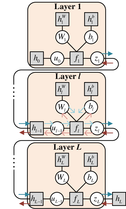
Figure 3: The structure of $\mathcal{G}_{r_{k}}$ ($r_{k}=1,\ldots,R_{k}$). The specific expression of factor nodes are summarized in Table I.

Factor	Distribution	Functional form
$h_{0}$	$p\left(\boldsymbol{u}_{0}^{r_{k}}|\boldsymbol{x}^{r_{k}}\right)$	$\prod_{i\in\mathcal{I}_{r_{k}}}\prod_{n=1}^{N_{0}}\delta\left(u_{0,ni}-x_{n}^{i}\right)$
$h_{l}$	$p\left(\boldsymbol{u}_{l}^{r_{k}}|\boldsymbol{z}_{l}^{r_{k}}\right)$	$\prod_{i\in\mathcal{I}_{r_{k}}}\prod_{m=1}^{N_{l}}\delta\left(u_{l,mi}-\zeta_{l}\left(z_{l,mi}\right)\right)$
$h_{L}$	$p\left(\boldsymbol{y}^{r_{k}}|\boldsymbol{z}_{l}^{r_{k}}\right)$	$\begin{cases}\prod_{i\in\mathcal{I}_{r_{k}}}\prod_{m=1}^{N_{L}}N\left(y_{m}^{i};z_{L,mi},v\right)&Regression\\ \prod_{i\in\mathcal{I}_{r_{k}}}\prod_{m\neq y^{i}}Q\left(\frac{z_{L,mi}-z_{L,y^{i}i}}{\sqrt{v}}\right)&Classification\end{cases}$
$h_{l}^{W}$	$p\left(\boldsymbol{W}_{l}\right)$	$\prod_{n=1}^{N_{l-1}}\left(\rho_{l,n}\prod_{m=1}^{N_{l}}N\left(W_{l,mn};\mu_{l,mn},v_{l,mn}\right)+\left(1-\rho_{l,n}\right)\prod_{m=1}^{N_{l}}\delta\left(W_{l,mn}\right)\right)$
$h_{l}^{b}$	$p\left(\boldsymbol{b}_{l}\right)$	$\prod_{m=1}^{N_{l}}\left(\rho_{l,m}^{b}N\left(b_{l,m};\mu_{l,m}^{b},v_{l,m}^{b}\right)+\left(1-\rho_{l,m}^{b}\right)\delta\left(b_{l,m}\right)\right)$
$f_{l}$	$p\left(\boldsymbol{z}_{l}^{r_{k}}|\boldsymbol{W}_{l},\boldsymbol{u}_{l-1}^{r_{k}},\boldsymbol{b}_{l}\right)$	$\prod_{i\in\mathcal{I}_{r_{k}}}\prod_{m=1}^{N_{l}}\delta\left(\boldsymbol{z}_{l,mi}-\left(\sum_{n=1}^{N_{l-1}}W_{l,mn}u_{l-1,ni}+b_{l,m}\right)\right)$

TABLE I: Factors, distributions and functional forms in Fig. 3.

Each iteration of the message passing procedure on the factor graph $\mathcal{G}_{r_{k}}$ in Fig. 3 consists of a forward message passing from the first layer to the last layer, followed by a backward message passing from the last layer to the first layer. However, the standard sum-product rule is infeasible on the DNN factor graph due to the high complexity. We propose DAMP to reduce complexity as will be detailed in Subsection III-B3. DAMP requires the prior distribution to be independent, so we follow turbo approach [25] to decouple the factor graph into Module $A$ and Module $B$ to compute messages with independent prior distribution and deal with group sparse prior separately.

III-B2 Turbo Framework to Deal with Group Sparse Prior

To achieve neuron-level pruning, each weight group is a column in weight matrix as discussed in Subsection II-B1. Specifically, we denote the $n$-th column in $\boldsymbol{W}_{l}$ by $\boldsymbol{W}_{l,n}$, where $l=1,\ldots,L,n=1,\ldots,N_{l-1}$, and the corresponding factor graph is shown in Fig. 4. The TDAMP algorithm iterates between two Modules $A$ and $B$. Module $A$ consists of factor nodes $f_{l}^{i},i\in\mathcal{I}_{r_{k}}$ that connect the weight parameters with the observation model, weight parameters $W_{l,mn},m=1,\ldots,N_{l}$, and factor nodes $h_{l,mn},m=1,\ldots,N_{l}$ that represent the extrinsic messages from Module $B$ denoted as $\triangle_{l,mn}^{B\rightarrow A}$. Module $B$ consists of factor node $h_{l,n}$ that represents the group sparse prior distribution, parameters $W_{l,mn},m=1,\ldots,N_{l}$, and factor nodes $h_{l,mn},m=1,\ldots,N_{l}$ that represent the extrinsic messages from Module $A$ denoted as $\triangle_{l,mn}^{A\rightarrow B}$. Module $A$ update the messages by performing DAMP algorithm with observations and independent prior distribution from Module $B$. Module $B$ updates the independent prior distributions for Module $A$ by performing sum-product message passing (SPMP) algorithm over the group sparse prior. In the following, we elaborate Module $A$ and Module $B$.

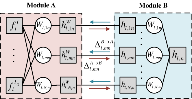
Figure 4: Turbo framework factor graph related to $\boldsymbol{W}_{l,n}$.

III-B3 DAMP in Module $A$

We compute the approximated marginal posterior distributions by performing DAMP. Based on turbo approach, in Module $A$, for $\forall l,m,n$, the prior factor nodes for weight matrices represent messages extracted from Module $B$:

$$h_{l,mn}^{W}\triangleq\triangle_{l,mn}^{B\rightarrow A}.$$

The factor graph for the $l$-th layer in $\mathcal{G}_{k}$ is shown in Fig. 5, where $u_{l-1,ni}$ and $z_{l,mi}$ represent the $n$-th element in $\boldsymbol{u}_{l-1}^{i}$ and $m$-th element in $\boldsymbol{z}_{l}^{i}$, respectively.

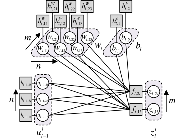
Figure 5: Detailed structure of the $l$-th layer related to the $i$-th sample, where we set $N_{l}=2,N_{l-1}=3$. The specific expressions of factor nodes are summarized in Table II.

Factor	Distribution	Functional form
$h_{l-1,ni}$	$\begin{cases}p\left(u_{0,ni}|x_{n}^{i}\right)&l=1\\ p\left(u_{l-1,ni}|z_{l-1,ni}\right)&l=2,\dots,L\end{cases}$	$\begin{cases}\delta\left(u_{0,ni}-x_{n}^{i}\right)&l=1\\ \delta\left(u_{l-1,ni}-\zeta_{l-1}\left(z_{l-1,ni}\right)\right)&l=2,\dots,L\end{cases}$
$f_{l,mi}$	$p\left(z_{l,mi}|\boldsymbol{W}_{l,n},\boldsymbol{u}_{l-1}^{i},b_{l,m}\right)$	$\delta\left(z_{l,mi}-\left(\sum_{n=1}^{N_{l-1}}W_{l,mn}u_{l-1,ni}+b_{l,m}\right)\right)$
$h_{l,m}^{b}$	$p\left(b_{l,m}\right)$	$\rho_{l,m}^{b}N\left(b_{l,m};\mu_{l,m}^{b},v_{l,m}^{b}\right)+\left(1-\rho_{l,m}^{b}\right)\delta\left(b_{l,m}\right)$
$h_{l,mn}^{W}$	$\exp\left(\triangle_{l,mn}^{B\rightarrow A}\right)$	$\rho_{l,mn}^{B\rightarrow A}N\left(W_{l,mn};\mu_{l,mn}^{B\rightarrow A},v_{l,mn}^{B\rightarrow A}\right)+\left(1-\rho_{l,mn}^{B\rightarrow A}\right)\delta\left(W_{l,mn}\right)$

TABLE II: Factors, distributions and functional forms in Fig. 5.

In the proposed DAMP, the messages between layers are updated in turn. For convenience, in the following, we denote by $\triangle_{a\rightarrow b}$ the message from node $a$ to $b$, and by $\triangle_{c}$ the marginal log-posterior computed at variable node $c$.

In forward message passing, layer $l=1,\dots,L$ output messages $\triangle_{f_{l,mi}\rightarrow z_{l,mi}}$ with input messages $\triangle_{h_{l-1,ni}\rightarrow u_{l-1,ni}}$:

$$\triangle_{h_{0,ni}\rightarrow u_{0,ni}}=\delta\left(u_{0,ni}-x_{n}^{i}\right),$$

and for $l=1,\dots,L-1$,

$$\triangle_{h_{l,ni}\rightarrow u_{l,ni}} =\log\int_{z_{l,ni}}\exp\left(\triangle_{f_{l,ni}\rightarrow z_{l,ni}}\right)$$

$$\times\delta\left(u_{l,ni}-\zeta_{l}\left(z_{l,ni}\right)\right).$$

In backward message passing, layer $l=L,\dots,1$ output messages $\triangle_{u_{l-1,ni}\rightarrow h_{l-1,ni}}$ with input messages $\triangle_{z_{l,mi}\rightarrow f_{l,mi}}$:

$$\triangle_{z_{L,mi}\rightarrow f_{L,mi}} =\log\int_{z_{l,m^{\prime}i},m^{\prime}\neq m}\exp\left(\sum_{m^{\prime}\neq m}\triangle_{f_{l,m^{\prime}i}\rightarrow z_{l,m^{\prime}i}}\right)$$

$$\times p\left(\boldsymbol{y}^{i}|\boldsymbol{z}_{L}^{i}\right),$$

and for $l=L-1,\dots,1$,

$$\triangle_{z_{l,mi}\rightarrow f_{l,mi}} =\log\int_{z_{l,mi}}\exp\left(\triangle_{u_{l,mi}\rightarrow h_{l,mi}}\right)$$

$$\times\delta\left(u_{l,mi}-\zeta_{l}\left(z_{l,mi}\right)\right).$$

Notice that the factor graph of a layer as illustrated in Fig. 5 has similar structure to the bilinear model discussed in [31]. Therefore, we follow the general idea of the BiG-AMP framework in [31] to approximate the messages within each layer. The detailed derivation is presented in the supplementary file of this paper, and the schedule of approximated messages is summarized in Algorithm 1. In particular, the messages $\triangle_{u_{l-1,ni}},\triangle_{z_{l,mi}}$ are related to nonlinear steps, which will be detailed in Appendix -A.

III-B4 SPMP in Module $B$

Module $B$ further exploits the structured sparsity to achieve structured model compression by performing the SPMP algorithm. Note that Module $B$ has a tree structure, and thus the SPMP is exact. For $\forall l,m,n$, the input factor nodes for Module $B$ are defined as output messages in Module $A$:

$$h_{l,mn} \triangleq\triangle_{l,mn}^{A\rightarrow B}=\triangle_{W_{l,mn}\rightarrow h_{l,mn}^{W}}.$$

Based on SPMP, we give the updating rule (25) for the output message as follows:

$$\exp\left(\triangle_{l,mn}^{B\rightarrow A}\right) \propto\int_{W_{l,m^{\prime}n},m^{\prime}\neq m}p\left(W_{l,n}\right)\exp\left(\sum_{m^{\prime}\neq m}\triangle_{l,mn}^{A\rightarrow B}\right)$$

$$\propto\rho_{l,mn}^{B\rightarrow A}N\left(W_{l,mn};\mu_{l,mn}^{B\rightarrow A},v_{l,mn}^{B\rightarrow A}\right)$$

$$+\left(1-\rho_{l,mn}^{B\rightarrow A}\right)\delta\left(W_{l,mn}\right),$$ (25)

where

$$\mu_{l,mn}^{B\rightarrow A}=\mu_{l,mn},v_{l,mn}^{B\rightarrow A}=v_{l,mn},$$

$$\rho_{l,mn}^{B\rightarrow A}=\frac{\rho_{l,n}}{\rho_{l,n}+\left(1-\rho_{l,n}\right)\prod_{m^{\prime}\neq m}\eta_{l,mn}},$$

$$\eta_{l,mn}=\frac{N\left(\mu_{l,mn}^{A\rightarrow B},v_{l,mn}^{A\rightarrow B}\right)}{N\left(\mu_{l,mn}^{A\rightarrow B}-\mu_{l,mn},v_{l,mn}^{A\rightarrow B}+v_{l,mn}\right)}.$$

The posterior distribution for $\boldsymbol{W}_{l,n}$ is given by (26), which will be used in Subsection III-B5 to update the prior distribution.

$$p\left(\boldsymbol{W}_{l,n}|\boldsymbol{D}^{r_{k}}\right) \propto p\left(\boldsymbol{W}_{l,n}\right)\times\exp\left(\sum_{m}\triangle_{W_{l,mn}\rightarrow h_{l,mn}^{W}}\right)$$

$$\propto\rho_{l,n}^{post}\prod_{m=1}^{N_{l}}N\left(W_{l,mn};\mu_{l,mn}^{post},v_{l,mn}^{post}\right)$$

$$+\left(1-\rho_{l,n}^{post}\right)\prod_{m=1}^{N_{l}}\delta\left(W_{l,mn}\right),$$ (26)

where

$$\rho_{l,n}^{post}=\frac{\rho_{l,n}}{\rho_{l,n}+\left(1-\rho_{l,n}\right)\prod_{m}\eta_{l,mn}},$$

$$\mu_{l,mn}^{post}=\frac{\frac{\mu_{l,mn}}{v_{l,mn}}+\frac{\mu_{l,mn}^{B\rightarrow A}}{v_{l,mn}^{B\rightarrow A}}}{\frac{1}{v_{l,mn}}+\frac{1}{v_{l,mn}^{B\rightarrow A}}},v_{l,mn}^{post}=\frac{1}{\frac{1}{v_{l,mn}}+\frac{1}{v_{l,mn}^{B\rightarrow A}}}.$$

III-B5 PasP Rule to Update Prior Distribution $p\left(\boldsymbol{\theta}\right)$

To accelerate convergence and fuse the information among minibatches, we update the joint prior distribution $p\left(\boldsymbol{\theta}\right)$ after processing each minibatch. Specifically, after updating the joint posterior distribution based on the $r_{k}$-th batch, we set the prior distribution as the posterior distribution. The mechanism is called PasP (27) mentioned in [27]:

$$p\left(\boldsymbol{\theta}\right)=\left(p\left(\boldsymbol{\theta}|\boldsymbol{D}^{r_{k}}\right)\right)^{\lambda},$$ (27)

where the posterior distributions for biases are computed through DAMP in Module $A$, while the posterior distributions for weights are computed through (26) in Module $B$. By doing so, the information from the all the previous minibatches are incorporated in the updated prior distribution. In practice, $\lambda$ plays a role similar to learning rate in SGD, and is typically set close to 1 [27]. For convenience, we fix $\lambda=1$ in simulations.

III-B6 Summary of the TDAMP Algorithm

To sum up, the proposed TDAMP algorithm at client $k$ is implemented as Algorithm 1, where $\tau_{max}$ represents maximum iteration number at each client.

Algorithm 1 TDAMP algorithm at client $k$

Input: Hyperparameters $\boldsymbol{\psi},v$, local dataset $\boldsymbol{D}^{k}$.

Output: $p\left(\boldsymbol{\theta}|\boldsymbol{D}^{k}\right),p\left(\boldsymbol{z}_{L}^{k}|\boldsymbol{D}^{k}\right)$

Initialization: Set prior distribution $p\left(\boldsymbol{\theta}\right)$ and likelihood function $p\left(\boldsymbol{D}^{k}|\boldsymbol{z}_{L}^{k}\right)$ based on $\boldsymbol{\psi}$ and $v$.

$\forall n,i:\triangle_{h_{0,ni}\rightarrow u_{0,ni}}=\log\delta\left(u_{0,ni}-x_{n}^{i}\right)$,

$\forall l,m:\triangle_{b_{l,m}\rightarrow h_{l,m}^{b}}=0$, $\forall l,m,n:\triangle_{W_{l,mn}\rightarrow h_{l,mn}^{W}}=0$, $\forall l,n,i:\triangle_{u_{l-1,ni}\rightarrow h_{l-1,ni}}=0$, $\forall l,m,n:\triangle_{s_{l,mi}}=0$.

1:  for $\tau=1,\ldots,\tau_{\max}$ do

2:     for $r_{k}=1,\ldots,R_{k}$ do

3:        Module $B$ (SPMP)

4:        Update output messages for Module $A$ $\forall l,m,n:\triangle_{l,mn}^{B\rightarrow A}$ as (25) and posterior distribution for weight groups $\forall l,n:p\left(\boldsymbol{W}_{l,n}|\boldsymbol{D}^{r_{k}}\right)$ as (26).

5:        Module $A$ (DAMP)

6:        Set prior distributions $\forall l,m,n:\triangle_{h_{l,mn}^{W}\rightarrow W_{l,mn}}=\triangle_{l,mn}^{B\rightarrow A},\forall l,m:\triangle_{h_{l,m}^{b}\rightarrow b_{l,m}}=p\left(b_{l,m}\right)$ and likelihood function $p\left(\boldsymbol{D}_{y}^{r_{k}}|\boldsymbol{z}_{L}^{r_{k}}\right)$ with noise variance $v$.

7:        %Forward message passing

8:        for $l=1,\ldots,L$ do

9:           Update input messages $\forall n,i:\triangle_{h_{l-1,ni}\rightarrow u_{l-1,ni}}$.

10:           Update posterior messages $\forall m,n,i:\triangle_{b_{l,m}},\triangle_{W_{l,mn}},\triangle_{u_{l-1,ni}}$.

11:           Update forward messages $\forall m,i:\triangle_{f_{l,mi}\rightarrow z_{l,mi}}$.

12:        end for

13:        %Backward message passing

14:        for $l=L,\ldots,1$ do

15:           Update input messages $\forall m,i:\triangle_{z_{l,mi}\rightarrow f_{l,mi}}$.

16:           Update posterior messages $\forall m,i:\triangle_{z_{l,mi}}$.

17:           Update aggregated backward messages $\forall m,n,i:\triangle_{b_{l,m}\rightarrow h_{l,m}^{b}},\triangle_{W_{l,mn}\rightarrow h_{l,mn}^{W}},\triangle_{u_{l-1,ni}\rightarrow h_{l-1,ni}}$.

18:        end for

19:        PasP

20:        Update prior distribution $p\left(\boldsymbol{\theta}\right)$ as (27).

21:     end for

22:  end for

23:  Output $p\left(\boldsymbol{\theta}|\boldsymbol{D}^{k}\right)=p\left(\boldsymbol{\theta}\right)$ and $p\left(\boldsymbol{z}_{L}^{k}|\boldsymbol{D}^{k}\right)\propto\exp\left(\sum_{m=1}^{N_{L}}\sum_{i\in\mathcal{I}_{k}}\triangle_{\boldsymbol{z}_{L,mi}}\right)$.

III-C Summary of the Entire Bayesian Federated Learning Algorithm

The entire EM-TDAMP Bayesian federated learning algorithm is summarized in Algorithm 2, where $T_{max}$ represents maximum communication rounds.

Algorithm 2 EM-TDAMP Bayesian Federated Learning Algorithm

Input: Training set $\boldsymbol{D}^{k},k=1,\ldots,K$, maximum rounds $T_{max}$.

Output: $p\left(\boldsymbol{\theta}|\boldsymbol{D}\right)$.

1:  Initialization: Hyperparameters $\boldsymbol{\psi},v$.

2:  for $t=1\ldots T_{max}$ do

3:     Clients

4:     for $k=1\cdots K$ do

5:        Update local posterior distribution $p\left(\boldsymbol{\theta}|\boldsymbol{D}^{k}\right)$ and $p\left(\boldsymbol{z}_{L}^{k}|\boldsymbol{D}^{k}\right)$ by performing TDAMP as in Algorithm 1 with input hyperparameters $\boldsymbol{\psi},v$.

6:        Extract $\boldsymbol{\varphi}^{k}$ from $p\left(\boldsymbol{\theta}|\boldsymbol{D}^{k}\right)$.

7:        Compute $\sigma^{k}$ through (19)/(22) in regression/classification model.

8:        Send $\boldsymbol{\varphi}^{k},\sigma^{k}$ to the central server.

9:     end for

10:     Central server

11:     Compute approximated posterior distribution $q\left(\boldsymbol{\theta}\right)$ through aggregation (9)-(11), and extract hyperparameters as $\boldsymbol{\psi}$.

12:     Compute noise variance $v$ based on $\sigma^{k}$s through (18)/(23) in regression/classification model.

13:     Send $\boldsymbol{\psi}$ and $v$ to the clients.

14:  end for

15:  $p\left(\boldsymbol{\theta}|\boldsymbol{D}\right)\approx q\left(\boldsymbol{\theta}\right)$.

IV Performance Evaluation

In this section, we evaluate the performance of the proposed EM-TDAMP through simulations. We consider two commonly used application scenarios with datasets available online: the Boston house price prediction and handwriting recognition, which were selected to evaluate the performance of our algorithm in dealing with regression and classification problems, respectively.

We consider group sparse prior and compare to three baseline algorithms: standard SGD, SGD with group sparse group regularizer [13] and group SNIP (for fair comparison, we extend SNIP [32] to prune neurons). For convenience, we use Adam optimizer [7] for the baseline algorithms.

Two cases are considered in the simulations. Firstly, we consider single client case to compare the EM-TDAMP and SGD-based algorithms without aggregation. Furthermore, we consider multiple clients case to prove the superiority of the aggregation mechanism proposed in E-step as mentioned in Subsection III-A1, compared to baseline algorithms with widely-used FedAvg algorithm [8] for aggregation.

Before presenting the simulation results, we briefly compare the complexity. Here we neglect element-wise operations and only consider multiplications in matrix multiplications, which occupies the main running time in both SGD-based algorithms and the proposed EM-TDAMP algorithm. It can be shown that both SGD and EM-TDAMP require $O\left(\tau_{max}I\sum_{l=1}^{L}N_{l-1}N_{l}\right)$ multiplications per round, and thus they have similar complexity orders.

In the following simulations, we will focus on comparing the convergence speed and converged performance of the algorithms. Specifically, we will show loss on the test data during training process to evaluate the convergence speed (group SNIP becomes standard Adam when $\rho=1$, and thus we set $\rho=0.5$ to show the training process) and also show the converged performance under varying sparsity/pruning ratios to compare the proposed algorithm with baseline algorithms comprehensively. To achieve the target group sparsity for SGD-type baseline algorithms, we need to manually prune the parameter groups based on energy after training [7]. When calculating the loss (NMSE for regression model and error for classification model) on test data for the proposed EM-TDAMP, we fix the parameters as posterior expectations (i.e., we use MMSE point estimate for the parameters). Each result is averaged on 10 experiments.

IV-A Description of Models

IV-A1 Boston Housing Price Prediction

For regression model, we train a DNN based on Boston housing price dataset. The training set consists of 404 past housing price, each associated with 13 relative indexes for prediction. For convenience, we set the batchsize as 101 in the following simulations. The test dataset contains 102 data. We set the architecture as follows: the network comprises three layers, including two hidden layers, each with 64 output neurons and ReLU activation, and an output layer with one output neuron. Before training, we normalize the data for stability. We evaluate the prediction performance using the normalized mean square error (NMSE) as the criterion.

IV-A2 Handwriting Recognition

For classification model, we train a DNN based on MNIST dataset, which is widely used in machine learning for handwriting digit recognition. The training set consists of 60,000 individual handwritten digits collected from postal codes, with each digit labeled from 0 to 9. The images are grayscale and represented as $28\times 28$ pixels. In our experiments, we set the batch size as 100. The test set consists of 10,000 digits. Before training, each digit is converted into a column vector and divided by the maximum value of 255. We use a two-layer network, where the first layer has 128 output neurons and ReLU activation function, while the second layer has 10 output neurons. After that, there is a softmax activation function for the baseline algorithms and Probit-product likelihood function for the proposed algorithm. We will use the error on test data to evaluate the performance.

IV-B Simulation Results

We start by evaluating the performance of EM-TDAMP in a single client scenario, with $K=1,\tau_{max}=1$. The training curves and test loss-sparsity curves for both regression and classification models are depicted in Fig. 6 and Fig. 7. The training curves demonstrate that the proposed EM-TDAMP achieves faster training speed and also the best performance after enough rounds. The test loss at different sparsity curves show that the proposed EM-TDAMP achieves the best performance especially when the compression ratio is high, which demonstrates that EM-TDAMP can better promote sparsity than the baseline algorithms. There are three main reasons. First, message passing procedure updates variance of the parameters during iterations, which makes inference more accurate after same rounds, leading to faster convergence. Second, the noise variance can be automatically learned based on EM algorithm, which can adaptively control the learning rate and avoid manually tuning of parameters. Third, the proposed EM-TDAMP prune the groups based on sparsity during training, which is more efficient than baseline methods that prune based on energy or gradients.

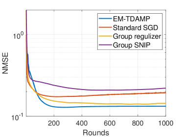
(a) Test NMSE in Boston housing price prediction.

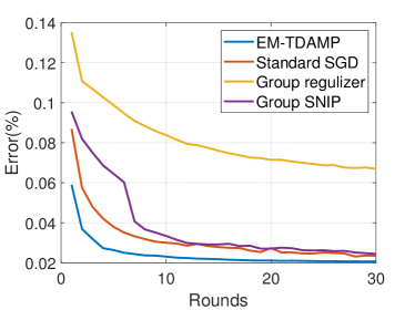
(b) Test error in handwriting recognition.

Figure 6: In singe client case, training curves of the proposed EM-TDAMP compared to baselines.

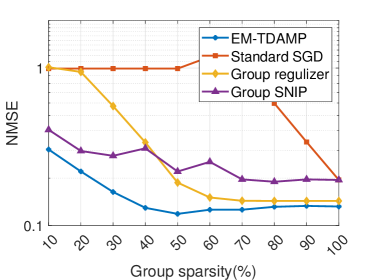
(a) Test NMSE in Boston housing price prediction.

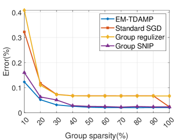
(b) Test error in handwriting recognition.

Figure 7: In singe client case, converged performance of proposed EM-TDAMP compared to baselines at different sparsity.

Next we verify the efficiency of the updating rule for noise variance in classification model discussed in Subsection III-A2. The Gumbel approximation (21) is illustrated in Fig. 8, where we compare the distributions when $t=1$ and $t=30$. Since scaling will not affect the solution for noise variance $v$ (21), we scale the distributions to set the maximum as 1 and only compare the shapes. We observe that both distributions have similar skewed shapes.

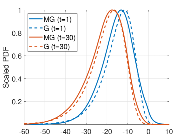
Figure 8: PDF of mixed Gaussian distribution and the approximated Gumbel distribution in (21), where $MG$ represents mixed Gaussian distribution and $G$ represents Gumbel distribution.

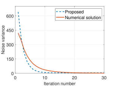
(a) Noise variance curve.

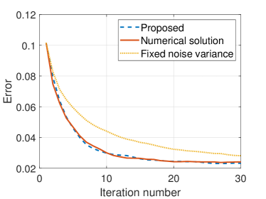
(b) Test error curve.

Figure 9: Comparison of different noise variance updating methods during training.

Furthermore, in Fig. 9, we compare the training performance achieved by different noise variance updating methods, where we set a large initialization to enhance the comparison during iterations. From Fig. 9a, we observe that the proposed updating rule is stable and can update noise variance similar to the numerical solution. Fig. 9b shows the proposed method achieves comparable training speed to the numerical solution, and both outperform the fixed noise variance case.

In the subsequent experiments, we consider multiple clients to evaluate the aggregation mechanism in federated learning scenarios. For convenience, we allocate an equal amount of data to each client, i.e., $I_{k}=\frac{I}{K}$ for $k=1,\cdots,K$. In Boston housing price prediction and handwriting recognition tasks, we set $K=4$ and $K=10$, respectively. To reduce communication rounds, we set $\tau_{max}=10$ in both cases (recall that $\tau_{max}$ refers to the number of inner iterations within each client in each round). The training curves and test loss-sparsity curves are shown in Fig. 10 and Fig. 11, respectively. Similar to the previous results, EM-TDAMP performs best among the algorithms, which proves the efficiency of the proposed aggregation method.

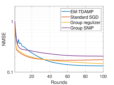
(a) Test NMSE in Boston housing price prediction.

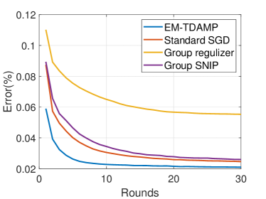
(b) Test error in handwriting recognition.

Figure 10: In multiple clients case, training curves of the proposed EM-TDAMP compared to baselines.

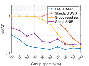
(a) Test NMSE in Boston housing price prediction.

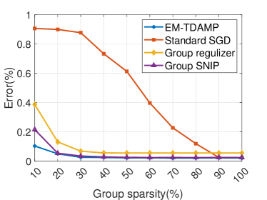
(b) Test error in handwriting recognition.

Figure 11: In multiple clients case, converged performance of proposed EM-TDAMP compared to baselines at different sparsity.

V Conclusions

In this work, we propose an EM-TDAMP algorithm to achieve Bayesian learning and compression in federated learning scenarios. In problem formulation, we propose a neuron-level sparse prior to promote group sparse structure and Gaussian noise at output to prevent numerical instability. Then, we derive the specific EM-TDAMP updating rules at the central server and the clients, respectively. At the central server, we propose EM algorithm, where the E-step computes the global posterior distributions through an efficient aggregation mechanism, and the M-step updates the hyperparameters to accelerate convergence. At the clients, we propose TDAMP to update the local posterior distributions, which consists of a Module $B$ to deal with group sparse prior distribution, a Module $A$ to enable efficient approximate message passing over DNN, and a PasP method to automatically tune the local prior distribution. Simulations show that the proposed EM-TDAMP can achieve faster convergence speed and better training performance compared to well-known structured pruning methods with Adam optimizer, especially when the compression ratio is high, making EM-TDAMP attractive to practical wireless federated learning scenarios. In the future, we will apply the proposed EM-TDAMP framework to design better training algorithm for more general DNNs, such as those with convolutional layers.

-A Nonlinear Steps

In this section, we mainly discuss the updating rules of $\triangle_{u_{l-1,ni}},\triangle_{z_{l,mi}}$ when related to nonlinear factors. Here we only provide the derivation for the messages, while the specific updating rules for expectation and variance will be detailed in the supplementary file.

-A1 ReLU Activation Function

ReLU is an element-wise function defined as (1). In this part, we give the updating rules for posterior messages of $u_{l,mi}$ and $z_{l,mi}$ for $\forall m,i$ when $\zeta_{l}\left(\cdot\right)$ is ReLU. Based on sum-product rule, we obtain:

$$\exp\left(\triangle_{u}\right) \propto\delta\left(u\right)Q\left(\frac{\mu_{f\rightarrow z}}{\sqrt{v_{f\rightarrow z}}}\right)N\left(\mu_{u\rightarrow h},v_{u\rightarrow h}\right)$$

$$+U\left(u\right)N\left(\mu_{f\rightarrow z}-\mu_{u\rightarrow h},v_{f\rightarrow z}+v_{u\rightarrow h}\right)$$

$$\times N\left(u;\frac{\mu_{u\rightarrow h}v_{f\rightarrow z}+\mu_{f\rightarrow z}v_{u\rightarrow h}}{v_{f\rightarrow z}+v_{u\rightarrow h}},\frac{v_{f\rightarrow z}v_{u\rightarrow h}}{v_{f\rightarrow z}+v_{u\rightarrow h}}\right),$$

$$\exp\left(\triangle_{z}\right) \propto U\left(-z\right)N\left(\mu_{u\rightarrow h},v_{u\rightarrow h}\right)N\left(z;\mu_{f\rightarrow z},v_{f\rightarrow z}\right)$$

$$+U\left(z\right)N\left(\mu_{u\rightarrow h}-\mu_{f\rightarrow z},v_{f\rightarrow z}+v_{u\rightarrow h}\right)$$

$$\times N\left(z;\frac{\mu_{u\rightarrow h}v_{f\rightarrow z}+\mu_{f\rightarrow z}v_{u\rightarrow h}}{v_{f\rightarrow z}+v_{u\rightarrow h}},\frac{v_{f\rightarrow z}v_{u\rightarrow h}}{v_{f\rightarrow z}+v_{u\rightarrow h}}\right),$$

where for convenience, we omit the subscript $l,mi$ and define $U\left(\cdot\right)$ as step function.

-A2 Probit-product Likelihood Function

Here, we briefly introduce the message passing related to output $z_{L,mi}$ for $\forall m,i$ in classification model. The factor graph of Probit-product likelihood function (6) is given in Fig. 12, where we omit $L,i$ for simplicity.

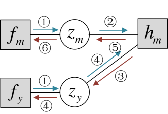
Figure 12: The factor graph of Probit-product likelihood function, where $h_{m}=Q\left(\frac{z_{m}-z_{y}}{\sqrt{v}}\right)$.

Firstly, to deal with $\triangle_{h_{m}\rightarrow z_{y}}$ for $\forall m\neq y$, we define

$$\triangle_{z_{y,m}} \triangleq\triangle_{h_{m}\rightarrow z_{y}}+\triangle_{f_{y}\rightarrow z_{y}}$$

$$=\log\int_{z_{m}}\exp\left(\triangle_{f_{m}\rightarrow z_{m}}+\triangle_{f_{y}\rightarrow z_{y}}\right)Q\left(\frac{z_{m}-z_{y}}{\sqrt{v}}\right)$$

$$=\log\left(\exp\left(\triangle_{f_{y}\rightarrow z_{y}}\right)Q\left(\frac{\mu_{f_{m}\rightarrow z_{m}}-z_{y}}{\sqrt{v+v_{f_{m}\rightarrow z_{m}}}}\right)\right),$$

where $\exp\left(\triangle_{z_{y,m}}\right)$ is a skew-normal distribution, and will be approximated as Gaussian based on moment matching. Then,

$$\triangle_{h_{m}\rightarrow z_{y}}=\triangle_{z_{y,m}}-\triangle_{f_{y}\rightarrow z_{y}}$$

is also approximated as logarithm of Gaussian. Next, based on sum-product rule, we obtain:

$$\triangle_{z_{y}}=\triangle_{f_{y}\rightarrow z_{y}}+\sum_{m\neq y}\triangle_{h_{m}\rightarrow z_{y}},$$

$$\triangle_{z_{y}\rightarrow h_{m}}=\triangle_{z_{y}}-\triangle_{h_{m}\rightarrow z_{y}}.$$

At last, for $m\neq y$, we approximate

$$\triangle_{z_{m}} =\triangle_{h_{m}\rightarrow z_{m}}+\triangle_{f_{m}\rightarrow z_{m}}$$

$$=\log\int_{z_{y}}\exp\left(\triangle_{z_{y}\rightarrow h_{m}}+\triangle_{f_{m}\rightarrow z_{m}}\right)Q\left(\frac{z_{m}-z_{y}}{\sqrt{v}}\right)$$

$$=\log\left(\exp\left(\triangle_{f_{m}\rightarrow z_{m}}\right)Q\left(\frac{\mu_{z_{y}\rightarrow h_{m}}-z_{y}}{\sqrt{v+v_{z_{y}\rightarrow h_{m}}}}\right)\right)$$

as logarithm of Gaussian based on moment matching again.

References

• [1] T. Li, A. K. Sahu, A. Talwalkar, and V. Smith, “Federated learning: Challenges, methods, and future directions,” IEEE Signal Processing Magazine, vol. 37, no. 3, pp. 50–60, 2020.
• [2] W. Oh and G. N. Nadkarni, “Federated learning in health care using structured medical data,” Advances in Kidney Disease and Health, vol. 30, no. 1, pp. 4–16.
• [3] A. Nguyen, T. Do, M. Tran, B. X. Nguyen, C. Duong, T. Phan, E. Tjiputra, and Q. D. Tran, “Deep federated learning for autonomous driving,” in 2022 IEEE Intelligent Vehicles Symposium (IV), pp. 1824–1830.
• [4] G. Ananthanarayanan, P. Bahl, P. BodÃk, K. Chintalapudi, M. Philipose, L. Ravindranath, and S. Sinha, “Real-time video analytics: The killer app for edge computing,” Computer, vol. 50, no. 10, pp. 58–67.
• [5] W. Y. B. Lim, N. C. Luong, D. T. Hoang, Y. Jiao, Y.-C. Liang, Q. Yang, D. Niyato, and C. Miao, “Federated learning in mobile edge networks: A comprehensive survey,” IEEE Communications Surveys & Tutorials, vol. 22, no. 3, pp. 2031–2063.
• [6] S. Ruder, “An overview of gradient descent optimization algorithms,” CoRR, vol. abs/1609.04747, 2016.
• [7] D. P. Kingma and J. Ba, “Adam: A method for stochastic optimization,” in 3rd International Conference on Learning Representations, ICLR 2015, San Diego, CA, USA, May 7-9, 2015, Conference Track Proceedings, 2015.
• [8] B. McMahan, E. Moore, D. Ramage, S. Hampson, and B. A. y Arcas, “Communication-efficient learning of deep networks from decentralized data,” in Proceedings of the 20th International Conference on Artificial Intelligence and Statistics, AISTATS 2017, 20-22 April 2017, Fort Lauderdale, FL, USA, ser. Proceedings of Machine Learning Research, vol. 54.   PMLR, 2017, pp. 1273–1282.
• [9] B. Hanin, “Which neural net architectures give rise to exploding and vanishing gradients?” in Advances in Neural Information Processing Systems, vol. 31, 2018.
• [10] S. Hochreiter, “The vanishing gradient problem during learning recurrent neural nets and problem solutions,” Int. J. Uncertain. Fuzziness Knowl. Based Syst., vol. 6, no. 2, pp. 107–116, 1998.
• [11] A. Choromanska, M. Henaff, M. Mathieu, G. B. Arous, and Y. LeCun, “The loss surfaces of multilayer networks,” in Proceedings of the Eighteenth International Conference on Artificial Intelligence and Statistics, AISTATS 2015, San Diego, California, USA, May 9-12, 2015, vol. 38.
• [12] M. Yuan and Y. Lin, “Model selection and estimation in regression with grouped variables,” Journal of the Royal Statistical Society: Series B (Statistical Methodology), vol. 68, no. 1, pp. 49–67, Feb. 2006.
• [13] S. Scardapane, D. Comminiello, A. Hussain, and A. Uncini, “Group sparse regularization for deep neural networks,” Neurocomputing, vol. 241, pp. 81–89, Jun. 2017.
• [14] S. Kim and E. P. Xing, “Tree-guided group lasso for multi-response regression with structured sparsity, with an application to eqtl mapping,” The Annals of Applied Statistics, vol. 6, no. 3, pp. 1095–1117.
• [15] K. Mitsuno, J. Miyao, and T. Kurita, “Hierarchical group sparse regularization for deep convolutional neural networks,” 2020 International Joint Conference on Neural Networks (IJCNN), pp. 1–8, 2020.
• [16] G. Litjens, T. Kooi, B. E. Bejnordi, A. A. A. Setio, F. Ciompi, M. Ghafoorian, J. A. W. M. van der Laak, B. van Ginneken, and C. I. Sánchez, “A survey on deep learning in medical image analysis,” Medical Image Analysis, vol. 42, pp. 60–88, Dec. 2017.
• [17] J. Kocic, N. S. Jovicic, and V. Drndarevic, “An end-to-end deep neural network for autonomous driving designed for embedded automotive platforms,” Sensors, vol. 19, no. 9, p. 2064, 2019.
• [18] X. Jiang, M. Osl, J. Kim, and L. Ohno-Machado, “Calibrating predictive model estimates to support personalized medicine,” Journal of the American Medical Informatics Association: JAMIA, vol. 19, no. 2, pp. 263–274, 2012.
• [19] H. Wang and D. Yeung, “A survey on bayesian deep learning,” ACM Comput. Surv., vol. 53, no. 5, pp. 108:1–108:37, 2021.
• [20] J. L. Puga, M. Krzywinski, and N. Altman, “Bayesian networks,” Nature Methods, vol. 12, no. 9, pp. 799–800, Sep. 2015.
• [21] J. T. Springenberg, A. Klein, S. Falkner, and F. Hutter, “Bayesian optimization with robust bayesian neural networks,” in Advances in Neural Information Processing Systems, vol. 29, 2016.
• [22] T. M. Fragoso and F. L. Neto, “Bayesian model averaging: A systematic review and conceptual classification,” International Statistical Review, vol. 86, no. 1, pp. 1–28, Apr. 2018.
• [23] M. Rani, S. B. Dhok, and R. B. Deshmukh, “A systematic review of compressive sensing: Concepts, implementations and applications,” IEEE Access, vol. 6, pp. 4875–4894, 2018.
• [24] A. Montanari, Graphical models concepts in compressed sensing.   Cambridge University Press, 2012, pp. 394–438.
• [25] J. Ma, X. Yuan, and L. Ping, “Turbo compressed sensing with partial dft sensing matrix,” IEEE Signal Processing Letters, vol. 22, no. 2, pp. 158–161, 2015.
• [26] P. Simard, D. Steinkraus, and J. Platt, “Best practices for convolutional neural networks applied to visual document analysis,” in Seventh International Conference on Document Analysis and Recognition, 2003. Proceedings., Aug. 2003, pp. 958–963.
• [27] C. Lucibello, F. Pittorino, G. Perugini, and R. Zecchina, “Deep learning via message passing algorithms based on belief propagation,” Machine Learning: Science and Technology, vol. 3, no. 3, p. 035005, Sep. 2022.
• [28] P. McCullagh, “Generalized linear models,” European Journal of Operational Research, vol. 16, no. 3, pp. 285–292, Jun. 1984.
• [29] T. Moon, “The expectation-maximization algorithm,” IEEE Signal Processing Magazine, vol. 13, no. 6, pp. 47–60, 1996.
• [30] L. Liu and F. Zheng, “A bayesian federated learning framework with multivariate gaussian product,” CoRR, vol. abs/2102.01936, 2021.
• [31] J. T. Parker, P. Schniter, and V. Cevher, “Bilinear generalized approximate message passing—part i: Derivation,” IEEE Transactions on Signal Processing, vol. 62, no. 22, pp. 5839–5853, Nov. 2014.
• [32] N. Lee, T. Ajanthan, and P. H. S. Torr, “Snip: single-shot network pruning based on connection sensitivity,” in 7th International Conference on Learning Representations, ICLR 2019, New Orleans, LA, USA, May 6-9, 2019, 2019.