Measurement-induced state transitions in dispersive qubit readout schemes

Abstract

The dispersive readout scheme enables quantum non-demolition measurement of superconducting qubits. An increased readout power can shorten the readout time and reduce the state discrimination error but can promote qubit transitions into higher noncomputational states. The ability to predict the onset of these measurement-induced state transitions can aid the optimization of qubit circuits and provide means for comparing the readout performance of different qubit types. Building upon the concept of dressed coherent states, we consider two straightforward metrics for determining the maximum number of photons that can be used for dispersive readout without causing state transitions. We focus on the fluxonium readout to demonstrate the independence of the metrics from any qubit-type-specific approximations. The dispersive readout of transmons and other superconducting qubits can be treated universally in the same fashion.

I Introduction

The dispersive readout of a superconducting qubit is realized by probing the qubit-state-dependent frequency of a linear resonator coupled to the qubit [1, 2], which enables a fast and high-fidelity single-shot measurement [3, 4, 5]. A short measurement duration is vital for implementing error correction codes such as the surface code [6], in which the data qubits must idle during the readout of the measure qubits and, thus, unavoidably accumulate errors due to intrinsic lifetime limitations [7]. Importantly, preserving the quantum non-demolitionness of the dispersive readout would guarantee that a qubit remains in a computational state after the measurement, allowing straightforward reset protocols [8, 9].

Several parameters determine the measurement rate, with the discussions typically framed in terms of the resonator dispersive shift $\chi$, the photon decay rate $\kappa$, and the average photon number $\bar{n}$. Numerical simulations can easily predict the first two quantities for a given qubit design. The optimal readout condition is often stated as $\kappa\approx 2\chi$, which maximizes the signal-to-noise ratio (SNR) for a fixed $\bar{n}$ in a linear resonator [10, 11]. Naïvely, increasing $\bar{n}$ should directly result in a higher SNR and thus in a better readout [10]. Unfortunately, in addition to a stronger resonator nonlinearity at larger $\bar{n}$, the qubit undergoes measurement-induced state transitions (MIST) when the number of photons exceeds a threshold value [12, 13, 14]. These transitions, sometimes referred to as qubit ionization in the context of transmon qubits escaping the Josephson potential well [15, 16], limit the measurement rate, degrade readout fidelity, and complicate qubit reset.

In this paper, we theoretically investigate the onset of MIST during the dispersive readout of superconducting qubits by focusing on two metrics that exhibit clear signatures of MIST. The first metric, the qubit purity, quantifies the qubit-resonator entanglement and was used in the past in numerical studies of qubit transitions and structural instabilities of the system dynamics [17, 14]. Time domain simulations reveal that the qubit purity remains very close to unity unless a state transition occurs as the number of readout photons increases. Our explanation of this sensitivity is based on the notion that away from MIST, the state of a driven qubit-resonator system would be close to a dressed coherent state [18, 19, 20, 21]. Perhaps surprisingly, such a state and its squeezed modifications were shown to be almost unentangled [21]. Further exploring this picture, we propose another metric that characterizes deviations in the drive matrix elements computed for the dressed coherent states. This metric, which is also very sensitive to MIST, bypasses time domain simulations and only requires accurate identification of the interacting qubit-resonator states. Throughout the paper, we focus on the case of a fluxonium qubit capacitively coupled to a resonator, although the analysis applies to the dispersive readout of any qubit type with a limited number of internal degrees of freedom.

The Jaynes-Cummings Hamiltonian [22] provides the starting point for the readout analysis of an ideal two-level qubit coupled to a resonator. In the dispersive regime, when the qubit-resonator coupling $g$ is much smaller than the qubit-resonator detuning $\Delta$, the resonator frequency is pulled by approximately $\pm g^{2}/\Delta$ with the sign determined by the qubit state [1]. The dispersive approximation breaks down when the photon number gets comparable to $n_{\textrm{crit}}=\Delta^{2}/(4g^{2})$, which corresponds to significant hybridization of the bare qubit-resonator states and the onset of resonator nonlinearity [11]. While $n_{\textrm{crit}}$ is often quoted as a characteristic of a qubit-resonator system, it does not set a hard limit on resonator occupation in a readout even when generalized for realistic multi-level qubits. In particular, $n_{\textrm{crit}}$ does not predict the likelihood of MIST, which, depending on system parameters, may occur at $\bar{n}$ drastically different from $n_{\rm crit}$. MIST in dispersive readout schemes are poorly understood and have been only studied in the context of transmon qubits as summarized below [13, 12, 14].

In a nutshell, the explanation of MIST in transmons is based on the resonances between energy levels of the interacting qubit-resonator system corresponding to different transmon states. The rotating wave approximation (RWA) simplifies the analysis for this qubit type with two distinct regimes defined by the transmon and resonator frequencies $\omega_{q}$ and $\omega_{r}$. When $\omega_{q}>\omega_{r}$, the level resonances within the same RWA strip are responsible for MIST due to the bending of the RWA strip over itself, which can result in a resonance between one of the two lowest qubit levels and a level near the edge of transmon’s cosine potential [12]. The onset of MIST often happens at relatively small photon numbers, depends strongly on the qubit-resonator detuning $\Delta$, and is highly sensitive to the transmon offset charge $n_{g}$ because of an increased sensitivity of the higher-lying qubit levels to $n_{g}$. The experimental data is consistent with a model based on the semiclassical equations of motions for the resonator field and the effective Schrödinger equation for the qubit [12]. In the opposite regime, when $\omega_{q}<\omega_{r}$, the resonances between levels in different RWA strips are found to be responsible for the transitions [13]. Crucially, while a simple model based on diagonalization of the Hamiltonian in RWA is sufficient to identify the resonances, non-RWA terms are necessary to explain the presence of the transitions between different RWA strips, pointing to the potential limitations of overly simplified models in predicting MIST. Notably, the transitions were observed at $\bar{n}$ several times larger than $n_{\rm crit}$, confirming that $n_{\rm crit}$ is not a reliable metric for estimating the limits on the dispersive readout power. In the $\omega_{q}<\omega_{r}$ regime, temporary resonance conditions due to fluctuations of $n_{g}$ may cause MIST only during specific time intervals [23].

A computationally expensive numerical study of the full dissipative dynamics of a transmon-resonator system under a strong measurement drive also revealed signatures of qubit transitions [14]. In that study, the Lindblad master equation with non-RWA terms in the Hamiltonian was integrated using large-scale computational accelerators, while a semiclassical approach was used to interpret the results. Similar to Refs. [13, 12], qubit transitions were attributed to level resonances occurring at specific photon numbers. The photon numbers were found to be strongly parameter-dependent and sometimes very small.

The onset of MIST in the other superconducting qubit types remains unexplored in part because of the inapplicability of the RWA-based approaches, such as in the case of fluxonia [24, 25, 26]. However, as with transmons, the dispersive shifts in fluxonium-resonator systems can be straightforwardly predicted with simulations matching experiments [27], and large photon numbers have been experimentally used for reading out fluxonia [28]. Yet, we are unaware of any practical tools for predicting the onset of MIST in fluxonia with the increase of $\bar{n}$.

Here, we investigate generic approaches to predicting MIST in superconducting qubits with a known Hamiltonian model using fluxonium as an example. The outline of the paper is as follows. In Sec. II, we introduce the Hamiltonian model, describe the procedure of numerical identification of its eigenstates, and discuss a particular example of a fluxonium spectrum prone to qubit transitions. In Sec. III, we simulate the dynamics for this specific example, discuss state transitions, and introduce metrics to catch the MIST effects. In Sec. IV, we investigate the dependence of MIST on the external magnetic flux and the resonator frequency. We conclude in Sec. V with general remarks. In Appendix A, we take a closer look at the qubit purity by calculating it in several limits. In Appendix B, the matrix element of raising operator $\hat{a}^{\dagger}$ is calculated using the perturbation theory. In Appendix C, we provide the simulation results for a transmon using parameters from Ref. [12] to further justify our approach.

II Model

II.1 Hamiltonian

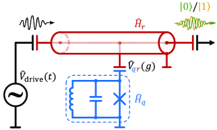
Figure 1: Schematic for dispersive readout of a superconducting qubit. A drive tone probes a readout resonator coupled to the qubit with coupling strength $g$. For illustrative purposes, we consider the case of capacitive coupling and fluxonium qubit, although the analysis can be generalized to inductive coupling and other superconducting qubit types.

We propose a universal method for identifying the onset of MIST in a general class of circuit quantum electrodynamics (cQED) setups (Fig. 1) described by the Hamiltonian

$$\hat{H}=\hat{H}_{q}+\hat{H}_{r}+\hat{V}_{qr}(g)+\hat{V}_{\textrm{drive}}(t)\,.$$ (1)

Here, $\hat{H}_{q}$ is a qubit Hamiltonian. In the main text, we examine a fluxonium qubit [24], for which

$$\hat{H}_{q}=4E_{C}\hat{n}^{2}+E_{L}\hat{\varphi}^{2}/2-E_{J}\cos(\hat{\varphi}-\varphi_{\textrm{ext}})\,,$$ (2)

while in Appendix C we include results for a transmon $\hat{H}_{q}$. In Eq. (2), $\hat{\varphi}$ and $\hat{n}$ are the normalized flux and charge operators satisfying $[\hat{\varphi},\hat{n}]=i$, and $E_{C}$, $E_{J}$, and $E_{L}$ are the charging, Josephson, and inductive energies. In addition, $\varphi_{\textrm{ext}}=2\pi\Phi_{\mathrm{ext}}/\Phi_{0}$, where $\Phi_{\textrm{ext}}$ is the external flux through the superconducting loop, $\Phi_{0}=h/(2e)$ is the flux quantum, $-e$ is the electron charge, and $h=2\pi\hbar$ is the Planck constant.

The second term in Eq. (1) describes the (linear) resonator and is written in terms of raising and lowering operators $\hat{a}^{\dagger}$ and $\hat{a}$ as $\hat{H}_{r}=\hbar\omega_{r}\hat{a}^{\dagger}\hat{a}$, where $\omega_{r}$ is the bare resonator frequency. The third term, $\hat{V}_{qr}(g)$, describes the qubit-resonator coupling, which is parametrized by a coupling strength $g$. For a pure capacitive coupling, considered in this paper, $\hat{V}_{qr}(g)=i\hbar g\hat{n}(\hat{a}^{\dagger}-\hat{a})$, while for pure inductive coupling $\hat{V}_{qr}(g)=\hbar g\hat{\varphi}(\hat{a}^{\dagger}+\hat{a})$. A readout drive of a fixed drive frequency $\omega_{\textrm{drive}}$ can be specified by

$$\hat{V}_{\textrm{drive}}(t)=2i\hbar\varepsilon(t)(\hat{a}^{\dagger}-\hat{a})\cos(\omega_{\textrm{drive}}t)\,,$$ (3)

where $\varepsilon(t)$ is the drive strength incorporating an initial raising stage. Generally, though, the time dependence of $\hat{V}_{\textrm{drive}}(t)$ can be more complex [29], and the drive is not necessarily monochromatic.

II.2 State identification

Let $\hat{H}_{\rm idle}(g)$ be Hamiltonian (1) without the drive term $\hat{V}_{\textrm{drive}}(t)$. When $g=0$, its eigenstates are trivially $\ket{k,n}=\ket{k}\otimes\ket{n}$ with total energies $E_{k,n}=E_{k}+n\hbar\omega_{r}$, where $\ket{k}$ is the $k$-th eigenstate of the qubit Hamiltonian $\hat{H}_{q}$ with energy $E_{k}$ and $\ket{n}$ is the $n$-th eigenstate of the resonator Hamiltonian $\hat{H}_{r}$, $k,n\geq 0$. When $g\neq 0$, the bare states $\ket{k,n}$ are no longer eigenstates of $\hat{H}_{\rm idle}(g)$. For convenience, we use the same indices to label the dressed eigenstates of the interacting Hamiltonian and corresponding eigenenergies as $\ket{\overline{k,n}}_{g}$ and $E_{\overline{{k,n}}}(g)$, or simply ${\ket{\overline{k,n}}}$ and $E_{\overline{k,n}}$ whenever we do not need to emphasize the value of $g$.

Ideally, a particular eigenstate of $\hat{H}_{\rm idle}(g)$ should be identified as $\ket{\overline{k,n}}_{g}$ when it is connected to $\ket{k,n}$ adiabatically, i.e., by varying $g$ slowly. In our numerical simulations, we use a labeling algorithm that we refer to as discrete adiabatic state identification (DASI). Starting with the noninteracting states $\ket{k,n}\equiv\ket{\overline{k,n}}_{g=0}$, the coupling strength $g$ is gradually increased in small discrete increments $\delta g$ until the value of interest is reached. At each new step, the updated interacting Hamiltonian $\hat{H}_{\rm idle}(g+\delta g)$ is diagonalized, and its eigenstates $\ket{\overline{k,n}}_{g+\delta g}$ are identified by maximizing the overlaps with $\ket{\overline{k,n}}_{g}$, the eigenstates of $\hat{H}_{\rm idle}(g)$. We emphasize that as a result, a state $\ket{\overline{k,n}}_{g}$ can have the largest overlap with a noninteracting state that is different from $\ket{k,n}$ due to nontrivial state hybridization. A simpler approach based on maximizing overlaps between dressed and bare states works well when only low-lying eigenstates are needed, such as when calculating dispersive shifts, but fails in general. We also find DASI to be more robust compared to the approach in which the states with one additional photon, i.e., $\ket{\overline{k,n+1}}$, are identified by finding the maximum overlap with the states generated by $a^{\dagger}$ acting on already identified states $\ket{\overline{k,n}}$ [14]. The approach of Ref. [14] has been recently improved in the algorithm of Ref. [30], where states $\ket{\overline{k,n+1}}$ are labeled by comparing their bare-qubit occupations with those of states $\ket{\overline{k,n}}$ and noticing that $E_{\overline{k,n+1}}$ must be close to $E_{\overline{k,n}}+\hbar\omega_{r}$.

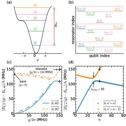
Figure 2: (a) Potential energy profile and single excitation energy level diagram for a fluxonium qubit at $\Phi_{\mathrm{ext}}/\Phi_{0}=0.1$ with the other system parameters specified in the text. The doubled bare resonator frequency is approximately equal to the transition frequency between states $\ket{0}$ and $\ket{4}$, leading to a resonant condition at a certain photon number. (b) Energy level diagram of the combined qubit-resonator system with no interaction ($g=0$). (c) Identification of the dressed eigenstates via a gradual sweep of coupling strength $g$ from zero (bare states) to $g/2\pi=150\,\mathrm{MHz}$ (black crosses). For clarity, only the dressed eigenenergies $E_{\overline{0,40}}$ and $E_{\overline{4,38}}$ relative to $E_{0,40}$ are shown. (d) Dressed eigenenergies $E_{\overline{0,n^{\prime}=n}}$ and $E_{\overline{4,n^{\prime}=n-2}}$ versus photon number $n$ for $g/2\pi=150\,\mathrm{MHz}$. The energies are shifted by $E_{0,n}=n\hbar\omega_{r}$ to remove the liner contribution proportional to $n$. The avoided-level-like crossing of the eigenladders at $n_{\textrm{cross}}=30$ leads to MIST when a comparable number of photons is used for readout.

Throughout the main text, we consider a fluxonium qubit with $E_{J}/h=4.0\,\mathrm{GHz}$, $E_{C}/h=1.0\,\mathrm{GHz}$, and $E_{L}/h=1.0\,\mathrm{GHz}$ capacitively coupled with coupling strength $g/2\pi=150\,\mathrm{MHz}$ to a resonator with $\omega_{r}/2\pi=7.0\,\mathrm{GHz}$. In our numerical simulations, carried out with the help of QuTiP software package [31, 32], the Hilbert space is composed of 20 qubit and 120 resonator levels, with the qubit eigenstates calculated by pre-diagonalizing $\hat{H}_{q}$ in the 50-level harmonic-oscillator basis of the capacitive and inductive terms. The DASI algorithm step size is $\delta g/2\pi=1.5\,\textrm{MHz}$.

We start by fixing the external flux at $\Phi_{\mathrm{ext}}/\Phi_{0}=0.1$, where the $\ket{0}-\ket{4}$ transition frequency $\omega_{04}=(E_{4}-E_{0})/\hbar$ is close to being twice the bare resonator frequency as seen in Fig. 2(a). This condition does not lead to features in the resonator dispersive shift but brings pairs of the states $\ket{0,n}$ and $\ket{4,n-2}$ into a resonance as depicted in Fig. 2(b). Figure 2(c) shows the evolution of the dressed eigenenergies from the corresponding bare states traced by the DASI algorithm for two particular dressed states, $\ket{\overline{0,40}}$ and $\ket{\overline{4,38}}$. We note the appearance of an avoided level crossing, where the naïve diabatic labeling procedure with a single coarse step $\delta g$ equal to $g$ would intermix the state labels.

The dressed eigenenergies corresponding to qubit indices $k=0$ and $k=4$ and different photon numbers are shown in Fig. 2(d) for $g/2\pi=150\,\mathrm{MHz}$. At small photon numbers, the spacing between the states corresponding to the qubit being in the ground ($k=0$) and the fourth excited state ($k=4$) is as large as $130\,\mathrm{MHz}$ while at photon numbers close to $n_{\textrm{cross}}=30$ this difference reduces to approximately $15\,\mathrm{MHz}$. Such reduction in spacing, together with the level repulsion, indicates strong hybridization between states $\ket{0,n}$ and $\ket{4,n-2}$ at $n\sim n_{\rm cross}$, suggesting that MIST would take place for qubit prepared in its ground state at the resonator occupation $\bar{n}\sim n_{\rm cross}$.

III Metrics for identifying measurement-induced transitions

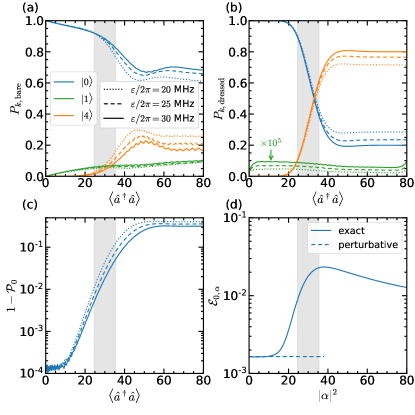
Figure 3: (a)–(c) Time evolution of the initial state $\ket{\overline{0,0}}$ in the presence of the resonant readout drive with $\varepsilon/2\pi=20$ (dotted lines), $25$ (dashed lines), and $30\,\textrm{MHz}$ (solid lines) for parameters of Fig. 2. (a) Probabilities $P_{0,\textrm{bare}}$ (blue), $P_{1,\textrm{bare}}$ (green), and $P_{4,\textrm{bare}}$ (orange) of finding the qubit in the bare states $\ket{0}$, $\ket{1}$, and $\ket{4}$ versus the average photon number $\expectationvalue{\hat{a}^{\dagger}\hat{a}}$. (b) Same but for $P_{k,\textrm{dressed}}$, where $P_{k,\textrm{dressed}}$ is the total probability of finding the system in one of the states $\ket{\overline{k,n}}$ (in the $k$-th dressed eigenladder). (c) Qubit purity error $1-\mathcal{P}_{0}$ versus $\expectationvalue{\hat{a}^{\dagger}\hat{a}}$. (d) Matrix elements error $\mathcal{E}_{0,\alpha}$ as defined by Eq. (6) for the ground state versus the average photon occupation $|\alpha|^{2}$ calculated exactly (solid line) and perturbatively (dashed line). In all panels, gray shading highlights $n_{\textrm{cross}}\pm\sqrt{n_{\textrm{cross}}}$ with $n_{\rm cross}$ defined in Fig. 2(d).

III.1 Qubit occupation probabilities

Time domain simulations of Hamiltonian (1) with drive term (3) reveal the expected MIST for parameters of Fig. 2(d). We ignore any dissipation for simplicity and solve the Schrödinger equation for a drive with $\omega_{\textrm{drive}}=\omega^{(0)}_{r}$ for the initial state $\ket{\overline{0,0}}$, where $\omega^{(k)}_{r}=(E_{\overline{k,1}}-E_{\overline{k,0}})/\hbar$ is the dressed resonator frequency for the qubit in $\ket{k}$. To reduce the stray population of states $\ket{\overline{k,n}}$ with a wrong qubit index $k\neq 0$, we choose an adiabatic drive [21] whose strength increases as $\sin(\pi t/2t_{\rm raise})$ in the interval $0<t<t_{\rm raise}$ with $t_{\rm raise}=20\,\textrm{ns}$ until it reaches a constant value $\varepsilon$. In Figs. 3(a)–3(c), the simulation results are plotted versus the simultaneously computed average resonator photon occupation $\expectationvalue{\hat{a}^{\dagger}\hat{a}}$.

Figure 3(a) shows probabilities of finding the qubit in various bare states defined as $P_{k,\textrm{bare}}\equiv\expectationvalue{\hat{\rho}_{q}}{k}=\sum_{n}\expectationvalue{\hat{\rho}}{k,n}$ for the $k$-th state, where $\hat{\rho}$ is the density matrix for the qubit-resonator system and

$$\hat{\rho}_{q}={\rm Tr}_{\rm res}\hat{\rho}$$ (4)

is the reduced density matrix for the qubit with the trace taken over the resonator degree of freedom. We find that $P_{0,\textrm{bare}}$ noticeably decreases while $P_{1,\textrm{bare}}$ increases even with a few photons. This behavior is unrelated to MIST since it is caused by the hybridization of bare states $\ket{0,n}$ and $\ket{1,n-1}$ that gets stronger with increasing $n$. A better metric is the probability of finding the interacting system in the $k$-th dressed eigenladder composed of dressed states $\ket{\overline{k,n}}$ with a fixed $k$. The physical interpretation of this is the probability of finding the qubit in its $k$-th dressed state. The dressed probabilities $P_{k,\textrm{dressed}}\equiv\sum_{n}\expectationvalue{\hat{\rho}}{\overline{k,n}}$ for $k=0,1$ and $4$ are shown in Fig. 3(b). We observe that $P_{0,\textrm{dressed}}\approx 1$ up to $\expectationvalue{\hat{a}^{\dagger}\hat{a}}\approx 20$, while $P_{1,\textrm{dressed}}$ is suppressed by roughly five orders of magnitude, indicating that the system remains in the correct eigenladder. In contrast, $P_{0,\textrm{dressed}}$ drops quickly between $n_{\rm cross}-\sqrt{n_{\rm cross}}$ and $n_{\rm cross}+\sqrt{n_{\rm cross}}$ and flattens again beyond this region. The drop is accompanied by a sharp increase in $P_{4,\textrm{dressed}}$, indicating a population exchange between the dressed states with $k=0$ and $k=4$, a clear MIST event. Similar observations can be made for bare probabilities $P_{0,\textrm{bare}}$ and $P_{4,\textrm{bare}}$, although the effect is obscured and hard to quantify because of the initial hybridization-induced slope.

A better indicator of MIST is hidden in the dependence of bare probabilities on the drive power. We note that both $P_{k,\mathrm{bare}}$ and $P_{k,\mathrm{dressed}}$ are practically independent of $\varepsilon$ at $\expectationvalue{\hat{a}^{\dagger}\hat{a}}<20$. They, however, depend on $\varepsilon$ at larger resonator occupation when the drive strength dictates how fast the system goes through the avoided-level-crossing-like region shaded in Fig. 3. A larger $\varepsilon$ reduces the adiabaticity of the evolution, i.e., the probability of traversing along the same eigenladder [the bottom eigenladder in Fig. 2(d)], but increases the probability of a diabatic-like transition into the $k=4$ eigenladder [the top eigenladder in Fig. 2(d)]. Therefore, the drive-strength order of bare and dressed state probabilities is reversed [compare blue solid, dashed, and dotted lines in Figs. 3(a) and 3(b)].

III.2 Qubit purity

Here, we discuss qubit-resonator entanglement by calculating the qubit purity $\mathcal{P}_{k}={\rm Tr}\hat{\rho}_{q}^{2}$, where index $k$ stands for the initial state $\ket{\overline{k,0}}$ at the start of a drive and $\hat{\rho}_{q}$ is given by Eq. (4). Figure 3(c) shows the “error” $1-\mathcal{P}_{0}$ as a function of the average photon occupation $\expectationvalue{\hat{a}^{\dagger}\hat{a}}$. Due to qubit-resonator coupling, the purity of the initial state $\ket{\overline{0,0}}$ is not exactly $1$. Somewhat counter-intuitively, $\mathcal{P}_{0}$ does not change appreciably during the initial stages of the drive despite the increased hybridized nature of eigenstates $\ket{\overline{0,n}}$ with $n\neq 0$. In the MIST region, however, $1-\mathcal{P}_{0}$ grows rapidly from about $10^{-3}$ at $\expectationvalue{\hat{a}^{\dagger}\hat{a}}\approx 20$ to about $10^{-1}$ at $\expectationvalue{\hat{a}^{\dagger}\hat{a}}\approx 40$, indicating a stronger entanglement of the qubit-resonator system. Similar observations for the purity were made for the transmon [14].

This behavior of the qubit-resonator entanglement is readily understood within the framework of the dressed coherent states [18, 19, 20], which are defined for an arbitrary coherent-state amplitude $\alpha$ as

$$\ket{\overline{k,\alpha}}=e^{-|\alpha|^{2}/2}\sum_{n}\frac{\alpha^{n}}{\sqrt{n!}}\ket{\overline{k,n}}.$$ (5)

A dressed coherent state approximates very well the state of an interacting qubit-resonator system generated by a classical microwave drive from the initial state $\ket{\overline{k,0}}$ [20]. In comparison to the product state $\ket{k,\alpha}=\ket{k}\otimes\ket{\alpha}$, where $\ket{\alpha}$ is the resonator coherent state, Eq. (5) shows that the system remains in the eigenladder for the $k$-th qubit state, in agreement with Fig. 3(b). As shown for the transmon, the states evolve primarily within the qubit eigenladder even when $|\alpha|^{2}>n_{\rm crit}$ with two corrections to Eq. (5): small leakage to neighboring eigenladders and squeezing of the correct eigenladder portion, caused by the qubit nonlinearity [21]. Importantly, in stark contrast with strongly hybridized eigenstates $\ket{\overline{k,n}}$, dressed coherent states (5) remain practically unentangled: for a large $|\alpha|^{2}$, $\ket{\overline{k,\alpha}}\approx\ket{q}\otimes\ket{\alpha}$ with some $\ket{q}=\sum_{k}c_{k}\ket{k}$ [21]. This also holds when Eq.(5) is corrected for squeezing [21]. Thus, purity is expected to remain close to unity in the dispersive and strong hybridization limits, provided the system predominantly stays in the correct eigenladder. In Appendix A, we illustrate this statement for Jaynes-Cummings Hamiltonian by calculating $\mathcal{P}_{0}$ analytically. In particular, we show that in the dispersive limit, the deviation of $\mathcal{P}_{0}$ from 1 is the second-order effect for eigenstates, but is the effect of only sixth order in the coupling strength for dressed coherent states defined by Eq. (5).

The initially weak increase of the purity error $1-\mathcal{P}_{0}$ seen in Fig. 3(c) is consistent with the expectation of the qubit-resonator system to remain in a state close to $\ket{\overline{0,\alpha}}$ and thus be almost unentangled. The subsequent rapid growth of $1-\mathcal{P}_{0}$ by two orders of magnitude is caused by a MIST event, which, according to Fig. 3(b), results in a substantial leakage to the $k=4$ eigenladder and thus breaks the dressed-coherent-state picture. The onset of this transition can be determined by computing the sensitivity of the purity error to the drive amplitude at a fixed $\expectationvalue{\hat{a}^{\dagger}\hat{a}}$, although the non-RWA terms can complicate the numerical evaluation of these sensitivities.

While both the probability of finding the system in a particular eigenladder [Fig. 3(b)] and the qubit purity [Fig. 3(c)] are sensitive MIST metrics, calculation of $P_{k,\mathrm{dressed}}$ requires both time domain simulations and identification of dressed states for large photon numbers. In comparison, $\mathcal{P}_{0}$ can be computed directly from the time-dependent density matrix $\hat{\rho}(t)$, expressed in the bare basis, eliminating the need for labeling dressed eigenstates. Therefore, the qubit purity (and other entanglement measures) can be used as a practical probe of MIST when doing the time domain simulations.

III.3 Dressed matrix elements of the drive

The exact shape of the purity error curves depends on the resonator ring-up protocol and photon loss. Here, we introduce another metric based on the matrix elements of $\hat{a}$ that does not require time domain simulations with a specific drive term. Instead, we now assume that the qubit-resonator system is already in a dressed coherent state $\ket{\overline{k,\alpha}}$ and check whether the dressed-coherent-state picture remains valid if an extra photon is added or removed. To this end, we define a simple error metric that quantifies to which extent the dressed coherent state is an eigenstate of bare $\hat{a}$:

$$\mathcal{E}_{k,\alpha}=\left|1-\frac{\expectationvalue{\hat{a}}{\overline{k,\alpha}}}{\alpha}\right|\,.$$ (6)

The metric is trivially zero for bare coherent states $\ket{k,\alpha}$ since $\hat{a}\ket{k,\alpha}=\alpha\ket{k,\alpha}$. For dressed states, it shows how close the operators $\hat{a}^{\dagger}$ and $\hat{a}$ are to their dressed versions $\hat{\bar{a}}^{\dagger}$ and $\hat{\bar{a}}$, where $\hat{\bar{a}}=\sum_{k,n}\sqrt{n+1}\ket{\overline{k,n}}\bra{\overline{k,n+1}}$. It is the condition $\hat{a}\approx\hat{\bar{a}}$ that results in the generation of dressed coherent states by $\hat{V}_{\rm drive}$ [21]; therefore, a large $\mathcal{E}_{k,\alpha}$ indicates the breakdown of the dressed-coherent-state picture and thus the onset of MIST.

We note that to compute $\mathcal{E}_{k,\alpha}$ numerically, special attention has to be paid to the signs of eigenstates at each step of the DASI algorithm: in addition to identifying eigenstates $\ket{\overline{k,n}}_{g+\delta g}$ by maximizing overlaps, we also fix their phases by requiring $\prescript{}{g}{\langle\overline{k,n}\ket{\overline{k,n}}}_{g+\delta g}$ to have positive real values. This way, numerically calculated $\ket{\overline{k,\alpha}}$ is well defined and not spoiled by the potential phase ambiguity of $\ket{\overline{k,n}}$.

In Fig. 3(d), we plot $\mathcal{E}_{0,\alpha}$ as a function of $|\alpha|^{2}$ computed for the same parameters as in other panels (solid line). We find an order-of-magnitude jump between $|\alpha|^{2}\approx 20$ and $|\alpha|^{2}\approx 40$, indicating the expected MIST in agreement with the time domain simulations. Due to state hybridization, $\mathcal{E}_{k,0}$ is not zero at $|\alpha|^{2}=0$ with the actual value closely matching the perturbative result, which is independent of $|\alpha|$ [dashed line in Fig. 3(d); calculated in Appendix B].

The practical advantage of the metric defined by Eq. (6) is that it requires only time-independent terms of Hamiltonian (1) and allows direct comparison of different qubit types regardless of the specifics of the drive and system losses.

IV Dependence on Hamiltonian parameters

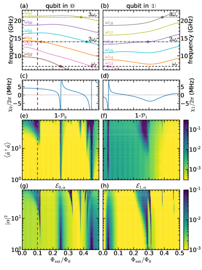
Figure 4: MIST dependence on the external flux $\Phi_{\mathrm{ext}}$ (horizontal axes) for a fluxonium initially in the ground (left) and first excited (right) states. (a), (b) Bare qubit and resonator transition frequencies with the resonance conditions highlighted by round markers. (c), (d) Dispersive shifts $\chi_{k}=(E_{\overline{k,1}}-E_{\overline{k,0}})/\hbar-\omega_{r}$, which diverge when $\omega_{r}$ matches one of the qubit transitions $\omega_{kk^{\prime}}$. (e), (f) Qubit purity errors $1-\mathcal{P}_{k}$ versus the average photon occupation $\expectationvalue{\hat{a}^{\dagger}\hat{a}}$ (vertical axes). (g), (h) Matrix element errors $\mathcal{E}_{k,\alpha}$ versus the average photon occupation $|\alpha|^{2}$ (vertical axes). The flux value of Figs. 2 and 3 is highlighted by vertical dashed lines in the left-column panels; other parameters are the same as in Figs. 2 and 3.

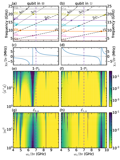
Figure 5: Same as Fig. 4, but for the dependence on the resonator frequency $\omega_{r}$ (horizontal axes) at the $\Phi_{\rm ext}=\Phi_{0}/2$ sweet spot. The value $\omega_{r}/2\pi=7\,\textrm{GHz}$ of Fig. 4 is highlighted by vertical dashed lines (the cross-sections along these lines are identical to the rightmost cross-sections in the corresponding panels of Fig. 4). Round markers in panels (a) and (b) label only those resonances for which the sweet-spot selection rules allow state transitions.

Here, we apply the ideas from Sec. III to explore MIST in a wider parameter space of the chosen fluxonium circuit. In Fig. 4, we investigate the dependence on the external flux $\Phi_{\textrm{ext}}$. We show the simulation results as a function of $\Phi_{\rm ext}$ for a qubit prepared in states $\ket{0}$ (left column) and $\ket{1}$ (right column). To build an intuition where MIST are possible, we start by plotting single-qubit transition frequencies $\omega_{kk^{\prime}}=(E_{k^{\prime}}-E_{k})/\hbar$ for $k=0$ and $k=1$ in Figs. 4(a) and 4(b). In these figures, the round markers indicate where $\omega_{kk^{\prime}}$ cross multiples of the bare resonator frequency $\omega_{r}$. “First-order” crossings $\omega_{kk^{\prime}}=\omega_{r}$ lead to divergences in the corresponding dispersive shift $\chi_{k}=\omega^{(k)}_{r}-\omega_{r}$ of the resonator frequency [27], clearly observed in Figs. 4(c) and 4(d). “Higher-order” crossings, e.g., those with $2\omega_{r}$ and $3\omega_{r}$, do not cause the dispersive shift to diverge but are expected to cause MIST. Ultimately, the anti-crossing of the $E_{\overline{0,n}}$ and $E_{\overline{4,n-2}}$ ladders in Fig. 2(d) occurs at a relatively small $n_{\rm cross}=30$ because $\omega_{04}$ is close to $2\omega_{r}$ [see Fig. 2(a) and the orange circle in Fig. 4(a)].

The intuition built upon the crossings of bare qubit and resonator frequencies is confirmed by simulations of the qubit purity $\mathcal{P}_{k}$ and the matrix-element error $\mathcal{E}_{k,\alpha}$. In Figs. 4(e) and 4(f), we show the qubit purity errors $1-\mathcal{P}_{0}$ and $1-\mathcal{P}_{1}$ for the starting states $\ket{\overline{00}}$ and $\ket{\overline{10}}$ as two-dimensional color maps versus $\Phi_{\rm ext}$ and $\expectationvalue{\hat{a}^{\dagger}\hat{a}}$. Both errors are simulated for $\varepsilon/2\pi=25$ MHz as described in Sec. III except that the drive frequency is $\omega_{\rm drive}=\omega_{r}^{(k)}$ for the initial state $\ket{\overline{k0}}$ to simplify simulations (the time-domain simulations do not correspond to an actual readout where $\omega_{\rm drive}$ is not qubit-state dependent). In Figs. 4(g) and 4(h), we show $\mathcal{E}_{0,\alpha}$ and $\mathcal{E}_{1,\alpha}$ versus $\Phi_{\rm ext}$ and $|\alpha|^{2}$. We brief on several observations. First, the features (i.e., the regions with increased errors) in the $1-\mathcal{P}_{k}$ panels mostly agree with the features in the $\mathcal{E}_{k,\alpha}$ panels. Second, the largest features in those panels, which occur at small photon number $\expectationvalue{\hat{a}^{\dagger}\hat{a}}$ and $|\alpha|^{2}$, correspond to divergences in the dispersive shifts. Third, the features appearing at crossings of single-qubit frequencies with $2\omega_{r}$, i.e., at $\Phi_{\rm ext}/\Phi_{0}\approx 0.1$ for a qubit in $\ket{0}$ and at $\Phi_{\rm ext}/\Phi_{0}\approx 0.3$ for a qubit in $\ket{1}$, are more pronounced with an earlier onset of MIST in comparison to the features corresponding to crossings with $3\omega_{r}$.

Figure 5 shows the same metrics calculated for the same parameters as Fig. 4 but as a function of the resonator frequency $\omega_{r}$ for the fluxonium parked at its half-integer sweet spot, $\Phi_{\rm ext}/\Phi_{0}=0.5$. We note that due to the selection rules at the sweet spot, i.e., $\bra{k}\hat{n}\ket{k^{\prime}}=0$ for two states $k$ and $k^{\prime}$ of the same parity, not every frequency collision observed in Figs. 5(a) and 5(b) leads to a divergence in the dispersive shift or an error growth in Figs. 5(e)–5(h). Even at higher orders, $\hat{V}_{qr}(g)$ mixes only the bare states $\ket{k,n}$ of the same combined parity $(-1)^{k+n}$ and, therefore, the parity of the dressed states is well defined. The avoided-level-like crossings such as the one shown in Fig. 2(d) occur only between dressed states of the same parity, and, thus, the resonance condition $\omega_{kk^{\prime}}=n\omega_{r}$ must be supplemented by the parity requirement $(-1)^{k-k^{\prime}}=(-1)^{n}$. Only such crossings are highlighted by round markers in Figs. 5(a) and 5(b), and the onset of the errors for each of these crossings is clearly visible in Figs. 5(e)–5(h).

V Summary and conclusions

Despite the well-established techniques for engineering dispersive shifts and coupling losses in circuit QED architectures, the task of the readout optimization remains partially a trial-and-error empirical endeavor. Crucially to this task, it is possible for qubit-resonator systems to have the same dispersive shifts and loss rates but behave differently with the increasing number of readout photons because of the measurement-induced state transitions. In this paper, we demonstrated how the qubit purity and the matrix element error computed for the dressed coherent states can be employed to identify parameter regimes favorable to implementing fast and high-fidelity readout protocols compatible with the deterministic reset.

The first metric, the qubit purity, requires the time domain simulations of the readout process to quantify the entanglement, while the second metric, the matrix element error, employs accurate identification of dressed states and quantifies the easiness with which the drive can increase the size of the dressed coherent state. Even though the system losses and the drive specifications do not enter the definition of the matrix element error, we expect this metric to be useful for identifying high-power readout regimes that are robust to minor drive calibration errors. Both metrics do not rely on any approximation such as RWA apart from the presumed (and practically desired) validity of the dressed coherent state picture. The metrics can be extended to the dressed squeezed states and be evaluated along the semiclassical trajectories in the resonator phase space the drive may produce. They allow a quantifiable comparison of different superconducting qubit types with respect to their performance in dispersive readout schemes and can provide universal guidelines for readout optimization.

Appendix A Qubit purity for two-level qubits

A.1 Model

Here, we build intuition of why the purity of the reduced qubit density matrix remains close to 1 for dressed coherent states (5) by considering a simple Jaynes-Cummings model in RWA:

$$\frac{\hat{H}_{\rm JC}}{\hbar}=\omega_{r}\hat{a}^{\dagger}\hat{a}-\frac{\omega_{q}}{2}\hat{\sigma}_{z}+g\left(\hat{a}\hat{\sigma}_{+}+\hat{a}^{\dagger}\hat{\sigma}_{-}\right)\,.$$ (7)

$\omega_{q}$ and $\omega_{r}$ are the bare qubit and resonator frequencies, and $g$ is the coupling strength. The purity error $1-\mathcal{P}_{0}$ calculated for this model numerically is shown in Fig. 6 for various values of the dimensionless coupling strength $\lambda=g/\Delta$, where $\Delta=\omega_{q}-\omega_{r}$. In this section, we calculate $\mathcal{P}_{0}$ for dressed coherent states analytically and derive a simple expression in the dispersive limit.

Hamiltonian (7) has a block-diagonal structure, with each block corresponding to a different RWA strip defined by the total excitation number. The exact diagonalization of the $2\times 2$ block with $n>0$ excitations gives the relation between dressed and bare states:

$$\ket{\overline{0,n}} =\cos\theta_{n}\ket{0,n}-\sin\theta_{n}\ket{1,n-1}\,,$$ (8)

$$\ket{\overline{1,n-1}} =\sin\theta_{n}\ket{0,n}+\cos\theta_{n}\ket{1,n-1}$$

with $\theta_{n}=\frac{1}{2}\tan^{-1}\left({2\lambda\sqrt{n}}\right)$. In the dispersive limit, we find

$$\theta_{n}=\lambda\sqrt{n}-\frac{4}{3}\left(\lambda\sqrt{n}\right)^{3}+\mathcal{O}\left(\left(\lambda\sqrt{n}\right)^{3}\right)\,.$$ (9)

In addition, the dressed state $\ket{\overline{0,0}}$ is exactly its bare version $\ket{0,0}$.

A.2 Dressed Fock states

We start by calculating the qubit purity for the exact eigenstate $\ket{\overline{0,n}}$ given by Eq. (8). To this end, we first write the full density matrix:

$$\hat{\rho}_{\overline{0,n}}=\cos^{2}\theta_{n}\outerproduct{0,n}{0,n}+\sin^{2}\theta_{n}\outerproduct{1,n-1}{1,n-1}\\ -\sin\theta_{n}\cos\theta_{n}\left(\outerproduct{0,n}{1,n-1}+\outerproduct{1,n-1}{0,n}\right)\,.$$ (10)

The reduced qubit density matrix is then given by

$$\hat{\rho}^{q}_{\overline{0,n}}={\rm Tr}_{\rm res}\hat{\rho}_{\overline{0,n}}=\cos^{2}\theta_{n}\outerproduct{0}{0}+\sin^{2}\theta_{n}\outerproduct{1}{1}\,,$$ (11)

which demonstrates that the qubit is not in a pure state. There are no off-diagonal terms in the reduced density matrix because the terms that are off-diagonal in the full density matrix (10) are also off-diagonal in the resonator index and do not survive the partial-trace operation. The purity of the reduced density matrix (11) is given by

$$\mathcal{P}_{{\overline{0,n}}}={\rm Tr}\left(\hat{\rho}^{q}_{\overline{0,n}}\right)^{2}=\cos^{4}\theta_{n}+\sin^{4}\theta_{n}\,.$$ (12)

In the dispersive limit of small $\theta_{n}$, we observe that $\mathcal{P}_{{\overline{0,n}}}\approx 1-2\sin^{2}\theta_{n}$. Thus, the qubit purity decreases twice as fast as the probability of finding the qubit in its bare ground state, which is simply $1-\sin^{2}\theta_{n}$. This cannot explain our numerical observations that purity remains close to $1$ up to relatively large photon numbers during the readout drive.

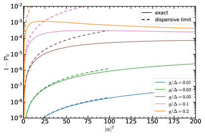
Figure 6: The purity error $1-\mathcal{P}_{0}$ calculated for the dressed coherent states $\ket{\overline{0,\alpha}}$ in the Jaynes-Cummings model (7) versus $|\alpha|^{2}$. The qubit purity is calculated exactly (solid lines) and using the dispersive result of Eq. (26) (dashed lines) for various values of the dispersive parameter $g/\Delta$.

A.3 Dressed coherent states

We now consider a generic state of the system within the same ground-state eigenladder:

$$\ket{\psi}=\sum_{n}C_{n}\ket{\overline{0,n}}\,,$$ (13)

where $\sum_{n}|C_{n}|^{2}=1$. A dressed coherent state of Eq. (5) is formed for $C_{n}={\alpha^{n}e^{-|\alpha|^{2}/2}}/{\sqrt{n!}}$. The full density matrix for state (13) is given by

$$\hat{\rho}_{\psi}=\sum_{n,n^{\prime}}C_{n}C^{*}_{n^{\prime}}\left(\cos\theta_{n}\ket{0,n}-\sin\theta_{n}\ket{1,n-1}\right)\\ \times\left(\cos\theta_{n^{\prime}}\bra{0,n^{\prime}}-\sin\theta_{n^{\prime}}\bra{1,n^{\prime}-1}\right)\,.$$ (14)

To find the reduced qubit density matrix $\hat{\rho}^{q}_{\psi}$, we only need to keep track of the bra-ket pairs with the same photon number. Such pairs come from the diagonal terms when $n=n^{\prime}$ and the off-diagonal terms when $n=n^{\prime}\pm 1$ (e.g., from the same or nearest-neighbor RWA strips). We thus find

$$\hat{\rho}^{q}_{\psi}=\rho^{q}_{00}\outerproduct{0}{0}+\rho^{q}_{11}\outerproduct{1}{1}+\rho^{q}_{01}\outerproduct{0}{1}+\left(\rho^{q}_{01}\right)^{*}\outerproduct{1}{0}\,,$$ (15)

where

$$\rho^{q}_{00}=\langle\cos^{2}\theta_{n}\rangle=\sum_{n}|C_{n}|^{2}\cos^{2}\theta_{n}\,,$$ (16)

$$\rho^{q}_{11}=\langle\sin^{2}\theta_{n}\rangle=\sum_{n}|C_{n}|^{2}\sin^{2}\theta_{n}\,,$$ (17)

and

$$\rho^{q}_{01}=-\sum_{n}C_{n}C^{*}_{n+1}\cos\theta_{n}\sin\theta_{n+1}\,.$$ (18)

This more generic expression contrasts with the reduced density matrix given in Eq. (11) for an eigenstate. While the diagonal matrix elements of $\hat{\rho}^{q}_{\psi}$ are simply averages of those in Eq. (11), off-diagonal elements appear only in the general expression (15). They arise from the joint contributions of the nearest-neighbor RWA strips and increase the qubit purity. For a state $\ket{\psi}$ that is almost evenly “spread out” over many RWA strips such as the dressed coherent state $\ket{\overline{0,\alpha}}$ with $|\alpha|^{2}\gg 1$, we have $C_{n}\sim C_{n+1}$ and $\theta_{n}\sim\theta_{n+1}$ for the dominant terms, so $|\rho^{q}_{01}|\sim\sqrt{\rho^{q}_{00}\rho^{q}_{11}}$. For a perfectly pure state, of course, $|\rho^{q}_{01}|=\sqrt{\rho^{q}_{00}\rho^{q}_{11}}$.

The generalization of Eq. (12) for the qubit purity is given by

$$\mathcal{P}_{\psi}={\rm Tr}\left(\hat{\rho}^{q}_{\psi}\right)^{2}=\left(\sum_{n}|C_{n}|^{2}\cos^{2}\theta_{n}\right)^{2}+\left(\sum_{n}|C_{n}|^{2}\sin^{2}\theta_{n}\right)^{2}+2\left|\sum_{n}C_{n}C^{*}_{n+1}\cos\theta_{n}\sin\theta_{n+1}\right|^{2}\\ =1-2\left(\sum_{n}|C_{n}|^{2}\cos^{2}\theta_{n}\right)\left(\sum_{n}|C_{n}|^{2}\sin^{2}\theta_{n}\right)+2\left|\sum_{n}C_{n}C^{*}_{n+1}\cos\theta_{n}\sin\theta_{n+1}\right|^{2}\,.$$ (19)

Since $\theta_{n}=0$ when $n=0$, we can shift index $n$ by one in the sum containing $\sin^{2}\theta_{n}$ to find that

$$\mathcal{P}_{\psi}=1-2\left[\sum_{n,n^{\prime}}\left(|C_{n}|^{2}|C_{n^{\prime}+1}|^{2}\cos^{2}\theta_{n}\sin^{2}\theta_{n^{\prime}+1}-C_{n}C^{*}_{n+1}C^{*}_{n^{\prime}}C_{n^{\prime}+1}\cos\theta_{n}\sin\theta_{n+1}\cos\theta_{n^{\prime}}\sin\theta_{n^{\prime}+1}\right)\right]\\ =1-\sum_{n,n^{\prime}}\left[|C_{n}|^{2}|C_{n^{\prime}+1}|^{2}\cos^{2}\theta_{n}\sin^{2}\theta_{n^{\prime}+1}+|C_{n^{\prime}}|^{2}|C_{n+1}|^{2}\cos^{2}\theta_{n^{\prime}}\sin^{2}\theta_{n+1}\right.\\ \left.-(C_{n}C^{*}_{n+1}C^{*}_{n^{\prime}}C_{n^{\prime}+1}+C_{n^{\prime}}C^{*}_{n^{\prime}+1}C^{*}_{n}C_{n+1})\cos\theta_{n}\sin\theta_{n+1}\cos\theta_{n^{\prime}}\sin\theta_{n^{\prime}+1}\right]\\ =1-\sum_{n,n^{\prime}}\left|C_{n}C_{n^{\prime}+1}\cos\theta_{n}\sin\theta_{n^{\prime}+1}-C_{n^{\prime}}C_{n+1}\cos\theta_{n^{\prime}}\sin\theta_{n+1}\right|^{2}$$ (20)

For a dressed coherent state $\ket{\overline{0,\alpha}}$, we thus have

$$\mathcal{P}_{\overline{0,\alpha}}=1-e^{-2|\alpha|^{2}}\sum_{n,n^{\prime}}\frac{|\alpha|^{2(n+n^{\prime}+1)}}{n!n^{\prime}!}\left(\frac{\cos\theta_{n}\sin\theta_{n^{\prime}+1}}{\sqrt{n^{\prime}+1}}-\frac{\cos\theta_{n^{\prime}}\sin\theta_{n+1}}{\sqrt{n+1}}\right)^{2}\,.$$ (21)

A.4 Dispersive limit

Let us find the leading contribution in the dispersive limit when $|\alpha|^{2}\ll\Delta^{2}/(4g^{2})$. We first notice that if we simply use $\theta_{n}\approx\lambda\sqrt{n}$ and $\cos\theta_{n}\approx 1$, the result would be $\mathcal{P}_{\overline{0,\alpha}}=1$, so we should consider higher-order corrections. Using Eq. (9) and keeping the terms up to the cubic power in $\lambda\sqrt{n}$, we find

$$\sin\theta_{n} =\lambda\sqrt{n}-\frac{3}{2}(\lambda\sqrt{n})^{3}+\mathcal{O}\left((\lambda\sqrt{n})^{3}\right)\,,$$ (22)

$$\cos\theta_{n} =1-\frac{1}{2}(\lambda\sqrt{n})^{2}+\mathcal{O}\left((\lambda\sqrt{n})^{3}\right)\,,$$

and

$$\frac{\cos\theta_{n}\sin\theta_{n^{\prime}+1}}{\sqrt{n^{\prime}+1}}=\lambda-\left[\frac{n}{2}+\frac{3(n^{\prime}+1)}{2}\right]\lambda^{3}+\mathcal{O}(\lambda^{3})\,,$$ (23)

so

$$\left(\frac{\cos\theta_{n}\sin\theta_{n^{\prime}+1}}{\sqrt{n^{\prime}+1}}-\frac{\cos\theta_{n^{\prime}}\sin\theta_{n+1}}{\sqrt{n+1}}\right)^{2}=(n-n^{\prime})^{2}\lambda^{6}+\mathcal{O}(\lambda^{6})\,.$$ (24)

Therefore, the effect of the qubit purity being different from one is in the sixth order in $g/\Delta$! In reality, deviations of the real state from the dressed-coherent state and deviations from the dispersive limit may give lower-order terms in $\lambda$.

To evaluate Eq. (21), we calculate

$$f(\alpha)=e^{-2|\alpha|^{2}}\sum_{n,n^{\prime}}\frac{|\alpha|^{2(n+n^{\prime}+1)}}{n!n^{\prime}!}(n-n^{\prime})^{2}=2e^{-|\alpha|^{2}}\sum_{n}\frac{|\alpha|^{2(n+1)}}{n!}n^{2}-2e^{-2|\alpha|^{2}}\left(\sum_{n}\frac{|\alpha|^{2n+1}}{n!}n\right)^{2}\\ =2e^{-|\alpha|^{2}}\sum_{n\geq 1}\frac{|\alpha|^{2(n+1)}}{(n-1)!}[(n-1)+1]-2e^{-2|\alpha|^{2}}\left(\sum_{n\geq 1}\frac{|\alpha|^{2n+1}}{(n-1)!}\right)^{2}=2|\alpha|^{4}\,.$$ (25)

Therefore, we find in the dispersive approximation

$$\mathcal{P}_{\overline{0,\alpha}}=1-2|\alpha|^{4}\left(\frac{g}{\Delta}\right)^{6}\,.$$ (26)

In Fig. 6, we show this approximate result by dashed lines.

A.5 Strong hybridization

Let us now consider the regime opposite to the dispersive approximation. Namely, we assume that $|\alpha|^{2}\gg\Delta^{2}/g^{2}$, so the Fock states hybridize very strongly and $\theta_{n}\sim\pi/4$ for relevant $n$. Using $\cos\theta_{n}=\sin\theta_{n}=1/2$ in Eq. (21), we find

$$\mathcal{P}_{\overline{0,\alpha}}=1-\frac{e^{-2|\alpha|^{2}}}{16}\sum_{n,n^{\prime}}\frac{|\alpha|^{2(n+n^{\prime}+1)}}{n!n^{\prime}!}\left(\frac{1}{\sqrt{n^{\prime}+1}}-\frac{1}{\sqrt{n+1}}\right)^{2}=1-\frac{e^{-2|\alpha|^{2}}}{8}\sum_{n,n^{\prime}}\frac{|\alpha|^{2n}|\alpha|^{2(n^{\prime}+1)}}{n!(n^{\prime}+1)!}\\ +\frac{e^{-2|\alpha|^{2}}}{8}\left(\sum_{n}\frac{|\alpha|^{2n+1}}{n!\sqrt{n+1}}\right)^{2}=1-\frac{1-e^{-|\alpha|^{2}}}{8}+\frac{1}{8}\left[1+e^{-|\alpha|^{2}}\sum_{n}\frac{|\alpha|^{2n}(|\alpha|-\sqrt{n+1})}{n!\sqrt{n+1}}\right]^{2}\,.$$ (27)

This expression suggests that even in this strong-coupling regime, the dressed coherent state is very close to being pure.

Appendix B Perturbation theory for matrix elements

Here, we calculate the matrix elements of $\hat{a}^{\dagger}$ for the states within the same eigenladder perturbatively, assuming charge coupling. For the same eigenladder, the first-order perturbation theory gives zero correction, and we need to do it in the second order. For fluxonium, the perturbation (qubit-resonator interaction) has the form

$$\hat{V}\equiv\hat{V}_{qr}(g)=-i\hbar g\hat{n}\left(\hat{a}-\hat{a}^{\dagger}\right)\,.$$ (28)

For the bare states, we have

$$\bra{k^{\prime},n^{\prime}}\hat{V}\ket{k,n}=igO_{k^{\prime},k}\left(\sqrt{n+1}\delta_{n^{\prime},n+1}-\sqrt{n}\delta_{n^{\prime},n-1}\right)\,,$$ (29)

where $O_{k^{\prime},k}=\hbar\bra{k^{\prime}}\hat{n}\ket{k}$ . Then, the dressed state up to the second order in $g$, including the normalization correction, has the form

$$\ket{\overline{k,n}}=\left[1-\frac{1}{2}\sum_{\{k^{\prime}n^{\prime}\}\neq\{kn\}}\frac{|\bra{k^{\prime},n^{\prime}}\hat{V}\ket{k,n}|^{2}}{\left(E_{k,n}-E_{k^{\prime},n^{\prime}}\right)^{2}}\right]\ket{k,n}+\sum_{\{k^{\prime},n^{\prime}\}\neq\{k,n\}}\frac{\bra{k^{\prime},n^{\prime}}\hat{V}\ket{k,n}}{E_{k,n}-E_{k^{\prime},n^{\prime}}}\ket{k^{\prime},n^{\prime}}\\ +\sum_{\{k^{\prime},n^{\prime}\},\{k^{\prime\prime},n^{\prime\prime}\}\neq\{k,n\}}\frac{\bra{k^{\prime},n^{\prime}}\hat{V}\ket{k^{\prime\prime},n^{\prime\prime}}\bra{k^{\prime\prime},n^{\prime\prime}}\hat{V}\ket{k,n}}{\left(E_{k,n}-E_{k^{\prime},n^{\prime}}\right)\left(E_{k,n}-E_{k^{\prime\prime},n^{\prime\prime}}\right)}\ket{k^{\prime},n^{\prime}}-\sum_{\{k^{\prime},n^{\prime}\}\neq\{k,n\}}\frac{\bra{k,n}\hat{V}\ket{k,n}\bra{k^{\prime},n^{\prime}}\hat{V}\ket{k,n}}{\left(E_{k,n}-E_{k^{\prime},n^{\prime}}\right)^{2}}\ket{k^{\prime},n^{\prime}}\,.$$ (30)

The last term in this expression is exactly zero because it contains a diagonal matrix element of $\hat{V}$. The other terms yield

$$\ket{\overline{k,n}}=\left\{1-\frac{g^{2}}{2}\sum_{k^{\prime}}|O_{k^{\prime},k}|^{2}\left[\frac{n+1}{(E_{k}-E_{k^{\prime}}-\omega_{r})^{2}}+\frac{n}{(E_{k}-E_{k^{\prime}}+\omega_{r})^{2}}\right]\right\}\ket{k,n}\\ +ig\sum_{k^{\prime}}O_{k^{\prime},k}\left[\frac{\sqrt{n+1}}{E_{k}-E_{k^{\prime}}-\omega_{r}}\ket{k^{\prime},n+1}-\frac{\sqrt{n}}{E_{k}-E_{k^{\prime}}+\omega_{r}}\ket{k^{\prime},n-1}\right]\\ -g^{2}\sum_{k^{\prime},k^{\prime\prime}}O_{k^{\prime},k^{\prime\prime}}O_{k^{\prime\prime},k}\left[\frac{\sqrt{(n+2)(n+1)}}{(E_{k}-E_{k^{\prime}}-2\omega_{r})(E_{k}-E_{k^{\prime\prime}}-\omega_{r})}\ket{k^{\prime},n+2}+\frac{\sqrt{n(n-1)}}{(E_{k}-E_{k^{\prime}}+2\omega_{r})(E_{k}-E_{k^{\prime\prime}}+\omega_{r})}\ket{k^{\prime},n-2}\right]\\ +g^{2}\sum_{k^{\prime}\neq k,k^{\prime\prime}}O_{k^{\prime},k^{\prime\prime}}O_{k^{\prime\prime},k}\left[\frac{n}{(E_{k}-E_{k^{\prime}})(E_{k}-E_{k^{\prime\prime}}+\omega_{r})}+\frac{n+1}{(E_{k}-E_{k^{\prime}})(E_{k}-E_{k^{\prime\prime}}-\omega_{r})}\right]\ket{k^{\prime},n}\,.$$ (31)

Thus, we find

$$\matrixelement{\overline{k,n^{\prime}}}{\hat{a}^{\dagger}}{\overline{k,n}}=\sqrt{n+1}\left\{1-\frac{g^{2}}{2}\sum_{k^{\prime}}|O_{k^{\prime},k}|^{2}\left[\frac{2n+3}{(E_{k}-E_{k^{\prime}}-\omega_{r})^{2}}+\frac{2n+1}{(E_{k}-E_{k^{\prime}}+\omega_{r})^{2}}\right]\right\}\delta_{n^{\prime},n+1}\\ +igO_{k,k}\left[\frac{\sqrt{(n+2)(n+1)}}{-\omega_{r}}\delta_{n^{\prime},n+2}-\frac{n}{\omega_{r}}\delta_{n^{\prime},n}-\frac{n+1}{-\omega_{r}}\delta_{n^{\prime},n}+\frac{\sqrt{(n+2)(n+1)}}{\omega_{r}}\delta_{n^{\prime},n+2}\right]\\ +g^{2}\sum_{k^{\prime}}|O_{k,k^{\prime}}|^{2}\left\{\left[\frac{(n+2)\sqrt{n+1}}{(E_{k}-E_{k^{\prime}}-\omega_{r})^{2}}+\frac{n\sqrt{n+1}}{(E_{k}-E_{k^{\prime}}+\omega_{r})^{2}}\right]\delta_{n^{\prime},n+1}-\frac{n\sqrt{n}\delta_{n^{\prime},n-1}+\sqrt{(n+3)(n+2)(n+1)}\delta_{n^{\prime},n+3}}{(E_{k}-E_{k^{\prime}}-\omega_{r})(E_{k}-E_{k^{\prime}}+\omega_{r})}\right\}\\ -g^{2}\sum_{k^{\prime}}|O_{k,k^{\prime}}|^{2}\left[\frac{\sqrt{(n+3)(n+2)(n+1)}}{(-2\omega_{r})(E_{k}-E_{k^{\prime}}-\omega_{r})}\delta_{n^{\prime},n+3}+\frac{\sqrt{n}(n-1)}{2\omega_{r}(E_{k}-E_{k^{\prime}}+\omega_{r})}\delta_{n^{\prime},n-1}\right]\\ -g^{2}\sum_{k^{\prime}}|O_{k,k^{\prime}}|^{2}\left[\frac{(n+1)\sqrt{n}}{(-2\omega_{r})(E_{k}-E_{k^{\prime}}-\omega_{r})}\delta_{n^{\prime},n-1}+\frac{\sqrt{(n+3)(n+2)(n+1)}}{2\omega_{r}(E_{k}-E_{k^{\prime}}+\omega_{r})}\delta_{n^{\prime},n+3}\right]\,.$$ (32)

We note that $O_{k,k}=0$ as the expectation value of the momentum operator in a one-dimensional bound state and that the terms with $\delta_{n^{\prime},n+3}$ cancel each other. Therefore, only the following matrix elements within the same eigenladder are nonzero in second order:

$$\matrixelement{\overline{k,n+1}}{\hat{a}^{\dagger}}{\overline{k,n}}=\sqrt{n+1}\left\{1+\frac{g^{2}}{2}\sum_{k^{\prime}}|O_{k,k^{\prime}}|^{2}\left[\frac{1}{(E_{k}-E_{k^{\prime}}-\omega_{r})^{2}}-\frac{1}{(E_{k}-E_{k^{\prime}}+\omega_{r})^{2}}\right]\right\}\,$$ (33)

and

$$\matrixelement{\overline{k,n-1}}{\hat{a}^{\dagger}}{\overline{k,n}}=g^{2}\sqrt{n}\sum_{k^{\prime}}|O_{kk^{\prime}}|^{2}\frac{E_{k}-E_{k^{\prime}}}{\omega_{r}(E_{k}-E_{k^{\prime}}-\omega_{r})(E_{k}-E_{k^{\prime}}+\omega_{r})}\,.$$ (34)

We next find the expectation value for the dressed coherent state:

$$\matrixelement{\overline{k,\alpha}}{\hat{a}^{\dagger}}{\overline{k,\alpha}}=e^{-|\alpha|^{2}}\sum_{n}\frac{|\alpha|^{2n}}{n!\sqrt{n+1}}\left[\alpha^{*}\matrixelement{\overline{k,n+1}}{\hat{a}^{\dagger}}{\overline{k,n}}+\alpha\matrixelement{\overline{k,n}}{\hat{a}^{\dagger}}{\overline{k,n+1}}\right]\\ =\alpha^{*}+\frac{g^{2}e^{-|\alpha|^{2}}}{2}\sum_{k^{\prime},n}|O_{k,k^{\prime}}|^{2}\frac{|\alpha|^{2n}}{n!}\left[\frac{\alpha^{*}}{(E_{k}-E_{k^{\prime}}-\omega_{r})^{2}}-\frac{\alpha^{*}}{(E_{k}-E_{k^{\prime}}+\omega_{r})^{2}}+\frac{2\alpha(E_{k}-E_{k^{\prime}})}{\omega_{r}(E_{k}-E_{k^{\prime}}-\omega_{r})(E_{k}-E_{k^{\prime}}+\omega_{r})}\right]\,.$$ (35)

At $\alpha\rightarrow 0$, this expectation value does not simply reduce to Eq. (33) but has a correction coming from Eq. (34). Finally, the matrix elements error (6) is given by

$$\mathcal{E}_{k,\alpha}=\frac{g^{2}}{2}\left|\sum_{k^{\prime}}|O_{k,k^{\prime}}|^{2}\left[\frac{1}{(E_{k}-E_{k^{\prime}}-\omega_{r})^{2}}-\frac{1}{(E_{k}-E_{k^{\prime}}+\omega_{r})^{2}}+\frac{2(E_{k}-E_{k^{\prime}})(\alpha/\alpha^{*})}{\omega_{r}(E_{k}-E_{k^{\prime}}-\omega_{r})(E_{k}-E_{k^{\prime}}+\omega_{r})}\right]\right|,$$ (36)

which is shown by the dashed line in Fig. 3(d). We thus find that $\mathcal{E}_{k,\alpha}$ calculated perturbatively depends on the phase of $\alpha$ but is independent of its magnitude. In simulations in this paper, we used $\alpha=|\alpha|e^{i\pi/2}$.

Appendix C Measurement-induced state transitions in a transmon qubit

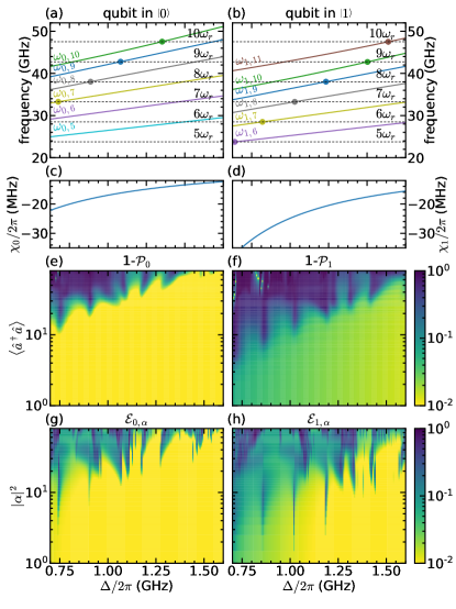
Figure 7: MIST in a transmon as a function of the qubit-resonator detuning $\Delta=\omega_{0,1}-\omega_{r}$ (horizontal axes). The notation and the panel arrangement are the same as in Figs. 4 and 5 of the main text. The simulations are done for parameters of Ref. [12] but for a fixed $n_{g}=0.2$ instead of averaging over its full range so that the transition frequency diagrams in panels (a) and (b) are not smeared out. Round markers in panels (a) and (b) label only those resonances for which state transitions are compatible with the selection rules of Eq. (38).

To ease the comparison with the recent transmon study [12], we include the simulations for a transmon qubit defined by Hamiltonian [33]

$$\hat{H}_{q}=4E_{C}(\hat{n}-n_{g})^{2}-E_{J}\cos\hat{\varphi}.$$ (37)

Here, $n_{g}$ is the offset charge, which can often be ignored in the transmon regime $E_{J}/E_{C}\gg 1$ but must be accounted for in a MIST study due to the sensitivity of higher-lying transmon levels to $n_{g}$ [12]. We intentionally do not assume any RWA and use the drive term of form (3) together with the qubit-resonator interaction term

$$\hat{V}_{qr}(g)=-\hbar g(\hat{a}-\hat{a}^{\dagger})(\hat{b}-\hat{b}^{\dagger})\,,$$ (38)

where the annihilation operator for the transmon is defined as $\hat{b}=\sum_{k}\sqrt{k+1}\ket{k}\bra{k+1}$.

We present our simulations in Fig. 7 for parameters of Ref. [12]: $\omega_{r}/2\pi=4.751\,\textrm{GHz}$, $E_{C}/h=0.194\,\textrm{GHz}$, and $k_{\rm eff}=0.048$ for the qubit-resonator coupling efficiency. For each value of the qubit-resonator detuning $\Delta=\omega_{0,1}-\omega_{r}$, varied in the range between 0.7 and 1.6 GHz, we calculate $E_{J}$ to match the qubit frequency $\omega_{0,1}$ and find the coupling strength $g=k_{\rm eff}\sqrt{\omega_{0,1}\omega_{r}}/2$. Although the averaging over $n_{g}$ is straightforward and is necessary to explain the experimental observations in Ref. [12], the simulations in Fig. 7 are done for a fixed $n_{g}=0.2$ to preserve the clarity of the transition frequency diagrams in Figs. 7(a) and 7(b). Even with a fixed $n_{g}$, the simulations agree very well with the experimental data of Ref. [12]. These simulations do not rely on the RWA approximation used in Ref. [12], although the RWA approximation can provide similar results in a faster computational runtime.

References

• Blais et al. [2004] A. Blais, R.-S. Huang, A. Wallraff, S. M. Girvin, and R. J. Schoelkopf, Cavity quantum electrodynamics for superconducting electrical circuits: An architecture for quantum computation, Phys. Rev. A 69, 062320 (2004).
• Blais et al. [2021] A. Blais, A. L. Grimsmo, S. M. Girvin, and A. Wallraff, Circuit quantum electrodynamics, Rev. Mod. Phys. 93, 025005 (2021).
• Johnson et al. [2012] J. E. Johnson, C. Macklin, D. H. Slichter, R. Vijay, E. B. Weingarten, J. Clarke, and I. Siddiqi, Heralded State Preparation in a Superconducting Qubit, Phys.Rev. Lett. 109, 050506 (2012).
• Walter et al. [2017] T. Walter, P. Kurpiers, S. Gasparinetti, P. Magnard, A. Potočnik, Y. Salathé, M. Pechal, M. Mondal, M. Oppliger, C. Eichler, and A. Wallraff, Rapid High-Fidelity Single-Shot Dispersive Readout of Superconducting Qubits, Phys. Rev. Applied 7, 054020 (2017).
• Swiadek et al. [2023] F. Swiadek, R. Shillito, P. Magnard, A. Remm, C. Hellings, N. Lacroix, Q. Ficheux, D. C. Zanuz, G. J. Norris, A. Blais, S. Krinner, and A. Wallraff, Enhancing dispersive readout of superconducting qubits through dynamic control of the dispersive shift: Experiment and theory, arXiv:2307.07765  (2023).
• Fowler et al. [2012] A. G. Fowler, M. Mariantoni, J. M. Martinis, and A. N. Cleland, Surface codes: Towards practical large-scale quantum computation, Phys. Rev. A 86, 032324 (2012).
• Acharya et al. [2023] R. Acharya, I. Aleiner, R. Allen, T. I. Andersen, M. Ansmann, F. Arute, K. Arya, A. Asfaw, J. Atalaya, R. Babbush, D. Bacon, J. C. Bardin, J. Basso, A. Bengtsson, S. Boixo, G. Bortoli, A. Bourassa, J. Bovaird, L. Brill, M. Broughton, B. B. Buckley, D. A. Buell, T. Burger, B. Burkett, N. Bushnell, Y. Chen, Z. Chen, B. Chiaro, J. Cogan, R. Collins, P. Conner, W. Courtney, A. L. Crook, B. Curtin, D. M. Debroy, A. Del Toro Barba, S. Demura, A. Dunsworth, D. Eppens, C. Erickson, L. Faoro, E. Farhi, R. Fatemi, L. Flores Burgos, E. Forati, A. G. Fowler, B. Foxen, W. Giang, C. Gidney, D. Gilboa, M. Giustina, A. Grajales Dau, J. A. Gross, S. Habegger, M. C. Hamilton, M. P. Harrigan, S. D. Harrington, O. Higgott, J. Hilton, M. Hoffmann, S. Hong, T. Huang, A. Huff, W. J. Huggins, L. B. Ioffe, S. V. Isakov, J. Iveland, E. Jeffrey, Z. Jiang, C. Jones, P. Juhas, D. Kafri, K. Kechedzhi, J. Kelly, T. Khattar, M. Khezri, M. Kieferová, S. Kim, A. Kitaev, P. V. Klimov, A. R. Klots, A. N. Korotkov, F. Kostritsa, J. M. Kreikebaum, D. Landhuis, P. Laptev, K.-M. Lau, L. Laws, J. Lee, K. Lee, B. J. Lester, A. Lill, W. Liu, A. Locharla, E. Lucero, F. D. Malone, J. Marshall, O. Martin, J. R. McClean, T. McCourt, M. McEwen, A. Megrant, B. Meurer Costa, X. Mi, K. C. Miao, M. Mohseni, S. Montazeri, A. Morvan, E. Mount, W. Mruczkiewicz, O. Naaman, M. Neeley, C. Neill, A. Nersisyan, H. Neven, M. Newman, J. H. Ng, A. Nguyen, M. Nguyen, M. Y. Niu, T. E. O’Brien, A. Opremcak, J. Platt, A. Petukhov, R. Potter, L. P. Pryadko, C. Quintana, P. Roushan, N. C. Rubin, N. Saei, D. Sank, K. Sankaragomathi, K. J. Satzinger, H. F. Schurkus, C. Schuster, M. J. Shearn, A. Shorter, V. Shvarts, J. Skruzny, V. Smelyanskiy, W. C. Smith, G. Sterling, D. Strain, M. Szalay, A. Torres, G. Vidal, B. Villalonga, C. Vollgraff Heidweiller, T. White, C. Xing, Z. J. Yao, P. Yeh, J. Yoo, G. Young, A. Zalcman, Y. Zhang, N. Zhu, and G. Q. AI, Suppressing quantum errors by scaling a surface code logical qubit, Nature 614, 676 (2023).
• Magnard et al. [2018] P. Magnard, P. Kurpiers, B. Royer, T. Walter, J.-C. Besse, S. Gasparinetti, M. Pechal, J. Heinsoo, S. Storz, A. Blais, and A. Wallraff, Fast and Unconditional All-Microwave Reset of a Superconducting Qubit, Phys. Rev. Lett. 121, 060502 (2018).
• Sunada et al. [2022] Y. Sunada, S. Kono, J. Ilves, S. Tamate, T. Sugiyama, Y. Tabuchi, and Y. Nakamura, Fast Readout and Reset of a Superconducting Qubit Coupled to a Resonator with an Intrinsic Purcell Filter, Phys. Rev. Applied 17, 044016 (2022).
• Gambetta et al. [2008] J. Gambetta, A. Blais, M. Boissonneault, A. A. Houck, D. I. Schuster, and S. M. Girvin, Quantum trajectory approach to circuit QED: Quantum jumps and the Zeno effect, Phys. Rev. A 77, 012112 (2008).
• Boissonneault et al. [2010] M. Boissonneault, J. M. Gambetta, and A. Blais, Improved Superconducting Qubit Readout by Qubit-Induced Nonlinearities, Phys. Rev. Lett. 105, 100504 (2010).
• Khezri et al. [2023] M. Khezri, A. Opremcak, Z. Chen, K. C. Miao, M. McEwen, A. Bengtsson, T. White, O. Naaman, D. Sank, A. N. Korotkov, Y. Chen, and V. Smelyanskiy, Measurement-induced state transitions in a superconducting qubit: Within the rotating-wave approximation, Phys. Rev. Applied 20, 054008 (2023).
• Sank et al. [2016] D. Sank, Z. Chen, M. Khezri, J. Kelly, R. Barends, B. Campbell, Y. Chen, B. Chiaro, A. Dunsworth, A. Fowler, E. Jeffrey, E. Lucero, A. Megrant, J. Mutus, M. Neeley, C. Neill, P. J. J. O’Malley, C. Quintana, P. Roushan, A. Vainsencher, T. White, J. Wenner, A. N. Korotkov, and J. M. Martinis, Measurement-Induced State Transitions in a Superconducting Qubit: Beyond the Rotating Wave Approximation, Phys. Rev. Lett. 117, 190503 (2016).
• Shillito et al. [2022] R. Shillito, A. Petrescu, J. Cohen, J. Beall, M. Hauru, M. Ganahl, A. G. Lewis, G. Vidal, and A. Blais, Dynamics of Transmon Ionization, Phys. Rev. Applied 18, 034031 (2022).
• Lescanne et al. [2019] R. Lescanne, L. Verney, Q. Ficheux, M. H. Devoret, B. Huard, M. Mirrahimi, and Z. Leghtas, Escape of a Driven Quantum Josephson Circuit into Unconfined States, Phys. Rev. Applied 11, 014030 (2019).
• Nojiri et al. [2024] Y. Nojiri, K. E. Honasoge, A. Marx, K. G. Fedorov, and R. Gross, Onset of transmon ionization in microwave single-photon detection, arXiv:2402.01884  (2024).
• Verney et al. [2019] L. Verney, R. Lescanne, M. H. Devoret, Z. Leghtas, and M. Mirrahimi, Structural instability of driven josephson circuits prevented by an inductive shunt, Phys. Rev. Applied 11, 024003 (2019).
• Sete et al. [2013] E. A. Sete, A. Galiautdinov, E. Mlinar, J. M. Martinis, and A. N. Korotkov, Catch-Disperse-Release Readout for Superconducting Qubits, Phys. Rev. Lett. 110, 210501 (2013).
• Sete et al. [2014] E. A. Sete, J. M. Gambetta, and A. N. Korotkov, Purcell effect with microwave drive: Suppression of qubit relaxation rate, Phys. Rev. B 89, 104516 (2014).
• Govia and Wilhelm [2016] L. C. G. Govia and F. K. Wilhelm, Entanglement generated by the dispersive interaction: The dressed coherent state, Phys. Rev. A 93, 012316 (2016).
• Khezri et al. [2016] M. Khezri, E. Mlinar, J. Dressel, and A. N. Korotkov, Measuring a transmon qubit in circuit QED: Dressed squeezed states, Phys. Rev. A 94, 012347 (2016).
• Jaynes and Cummings [1963] E. Jaynes and F. Cummings, Comparison of quantum and semiclassical radiation theories with application to the beam maser, Proceedings of the IEEE 51, 89 (1963).
• Hirasaki et al. [2024] Y. Hirasaki, S. Daimon, N. Kanazawa, T. Itoko, M. Tokunari, and E. Saitoh, Dynamics of measurement-induced state transitions in superconducting qubits, arXiv:2402.05409  (2024).
• Manucharyan et al. [2009] V. E. Manucharyan, J. Koch, L. I. Glazman, and M. H. Devoret, Fluxonium: Single Cooper-pair circuit free of charge offsets, Science 326, 113 (2009).
• Nguyen et al. [2019] L. B. Nguyen, Y.-H. Lin, A. Somoroff, R. Mencia, N. Grabon, and V. E. Manucharyan, High-Coherence Fluxonium Qubit, Phys. Rev. X 9, 041041 (2019).
• Nguyen et al. [2022] L. B. Nguyen, G. Koolstra, Y. Kim, A. Morvan, T. Chistolini, S. Singh, K. N. Nesterov, C. Jünger, L. Chen, Z. Pedramrazi, B. K. Mitchell, J. M. Kreikebaum, S. Puri, D. I. Santiago, and I. Siddiqi, Blueprint for a High-Performance Fluxonium Quantum Processor, PRX Quantum 3, 037001 (2022).
• Zhu et al. [2013] G. Zhu, D. G. Ferguson, V. E. Manucharyan, and J. Koch, Circuit QED with fluxonium qubits: Theory of the dispersive regime, Phys. Rev. B 87, 024510 (2013).
• Gusenkova et al. [2021] D. Gusenkova, M. Spiecker, R. Gebauer, M. Willsch, D. Willsch, F. Valenti, N. Karcher, L. Grünhaupt, I. Takmakov, P. Winkel, D. Rieger, A. V. Ustinov, N. Roch, W. Wernsdorfer, K. Michielsen, O. Sander, and I. M. Pop, Quantum Nondemolition Dispersive Readout of a Superconducting Artificial Atom Using Large Photon Numbers, Phys. Rev. Applied 15, 064030 (2021).
• McClure et al. [2016] D. T. McClure, H. Paik, L. S. Bishop, M. Steffen, J. M. Chow, and J. M. Gambetta, Rapid driven reset of a qubit readout resonator, Phys. Rev. Appl. 5, 011001 (2016).
• Goto and Koshino [2024] S. Goto and K. Koshino, Labeling eigenstates of qubit-cavity systems based on the continuity of qubit occupancy: Detecting resonances to higher excited qubit states, arXiv:2401.16666  (2024).
• Johansson et al. [2012] J. R. Johansson, P. D. Nation, and F. Nori, QuTiP: An open-source Python framework for the dynamics of open quantum systems, Comp. Phys. Comm. 183, 1760 (2012).
• Johansson et al. [2013] J. R. Johansson, P. D. Nation, and F. Nori, QuTiP 2: A Python framework for the dynamics of open quantum systems, Comp. Phys. Comm. 184, 1234 (2013).
• Koch et al. [2007] J. Koch, T. M. Yu, J. Gambetta, A. A. Houck, D. I. Schuster, J. Majer, A. Blais, M. H. Devoret, S. M. Girvin, and R. J. Schoelkopf, Charge-insensitive qubit design derived from the Cooper pair box, Phys. Rev. A 76, 042319 (2007).