Data Distribution-based Curriculum Learning

Abstract

The order of training samples can have a significant impact on the performance of a classifier. Curriculum learning is a method of ordering training samples from easy to hard. This paper proposes the novel idea of a curriculum learning approach called Data Distribution-based Curriculum Learning (DDCL). DDCL uses the data distribution of a dataset to build a curriculum based on the order of samples. Two types of scoring methods known as DDCL (Density) and DDCL (Point) are used to score training samples thus determining their training order. DDCL (Density) uses the sample density to assign scores while DDCL (Point) utilises the Euclidean distance for scoring. We evaluate the proposed DDCL approach by conducting experiments on multiple datasets using a neural network, support vector machine and random forest classifier. Evaluation results show that the application of DDCL improves the average classification accuracy for all datasets compared to standard evaluation without any curriculum. Moreover, analysis of the error losses for a single training epoch reveals that convergence is faster when using DDCL over the no curriculum method.

I Introduction

Classification tasks in supervised machine learning use various techniques to create classifiers suited to the problem. Some of the widely used techniques are neural networks, support vector machines (SVM) and decision trees [1]. Neural networks are biologically inspired computing systems [2] that are widely used as classifiers due to their ability to learn and improve their performance through the use of data and experience. SVMs use a threshold to classify a data sample as belonging to one class or another class [3]. This is done by starting with the training data in a lower dimension and then moving to a higher dimension. The higher dimension data is then separated into groups that represent each class. Decision trees perform classification by using a tree-like structure made up of smaller decisions to make an overall decision for a given input. Multiple decision trees are often combined to create an ensemble classifier known as a Random Forest classifier [4].

The performance of these classifiers are dependent on the quality of data used and the robustness of training algorithms. Some of the factors that affect the quality of data are inaccurate, inconsistent, imbalanced, duplicate, missing and outlier samples in a dataset [5, 6]. Studies on the quality of data have shown that these properties may lead to a significant degradation in prediction performance and cause instability in learning due to high bias and/or high variance [5, 7].

To reduce the negative impact of these factors, the training algorithms applied to datasets are often designed to guide the learning model towards optimum performance [8, 9, 10]. Gradient descent is the most common method of optimising a neural network due to its fast convergence towards the minimum error [11]. Variants of gradient descent such as batch gradient descent, stochastic gradient descent (SGD) and mini batch gradient descent exist for use with specific problem scenarios. These problems may favour computation speed, data size or a balance of speed and size as frequently seen in practice [12]. Support vector machines are optimised by selecting a value for the C hyperparameter and the method of optimising its kernel varies according to the kernel used. The Radial Basis Function (RBF) kernel is commonly used in a SVM and it is optimised by selecting the gamma ($\gamma$) hyperparameter. Both of these hyperparameters can be found using several search algorithms including trees of Parzen estimators, particle swarm optimization and Bayesian optimisation. Recent findings have concluded that the first two algorithms provide better hyperparameter values with a lower execution time compared to Bayesian optimisation which has a very high computational cost [13]. In a random forest classifier, the number of decision trees (estimators) and the number of features required to split a tree are hyperparameters that are optimised [14].

Furthermore, the data distribution plays a major role in obtaining quality predictions from classifiers. When using the same data, a particular data distribution of training data can provide better results compared to another data distribution. Research has shown that the choice of distribution can cause an overall low bias or high bias for the same training data and also lead to poor performance without being apparent [15, 16]. This bias can have a significant impact on the model’s performance which can be critical in medical applications [15, 17].

Once the distribution of data is known, a decision can be made on how data samples are selected from the dataset for optimal results. This decision may include using a specific criteria for selecting samples in a particular order. The process of selectively choosing samples from a dataset as well as determining their order is known as creating a curriculum.

Using a curriculum for improving performance of a machine learning model is known as curriculum learning and it is typically applied on the order of training data samples. Curriculum learning enhances training of a model by starting with simple concepts and then gradually introducing difficult concepts as training progresses [18]. It is inspired by how humans are taught through curriculums in an education system by receiving basic education during childhood and then moving on to advanced education in adulthood [19, 20].

Curriculum learning has been applied to various problems achieving excellent results in the areas of image classification [21, 22], face recognition [23], visual attribute classification [24] and imbalanced data classification [25]. It has also been successfully used to improve performance of existing systems that use machine learning including unsupervised domain adaptation [26], transfer learning [27, 28] and reinforcement learning [29, 30].

In this paper, we propose a data distribution based curriculum learning approach for classification tasks. The proposed approach first determines the distribution of data and then information from the distribution is used to build a curriculum based on the order of samples. The approach is then evaluated on multiple datasets with classifiers based on three different types of widely used learning methods: neural networks, SVM and random forest classifier. The remainder of the paper is organised as follows. Section II provides a background on curriculum learning and related learning approaches as well as applications of curriculum learning to various problems. The proposed curriculum learning approach is discussed in Section III and Section IV outlines its experimental evaluation. Section V examines the experiment results while Section VI provides concluding remarks.

II Background

The concept of using a curriculum in machine learning was introduced by Bengio et al. in 2009 [18]. Their work defined curriculum learning as a training strategy where fewer simple concepts are presented in order at the beginning with greater complex concepts introduced at later stages. The authors conducted experiments on shape recognition and language modelling for scenarios with and without a curriculum. Experiment results showed that by using a curriculum, faster training and better convergence can be achieved.

Kumar et al. [31] built upon the concepts introduced by Bengio et al. by proposing self-paced learning (SPL), a training strategy that also suggested presenting training samples ordered from simple to complex. The main difference between SPL and curriculum learning was the process of defining the difficulty of a sample. In SPL, the current learning progress of a model was considered for selecting the next sample whereas curriculum learning relied on a pre-determined fixed curriculum. The authors conducted experiments that showed their proposed method outperforming the state of the art method.

Years later, Jiang et al. proposed a framework called self-paced curriculum learning (SPCL) that sought to unify the ideas of curriculum learning and self-paced learning [32]. They reasoned that both types of learning have drawbacks; The curriculum in curriculum learning is heavily reliant on the quality of fixed pre-determined prior knowledge and ignores feedback about the learner. In self-paced learning, the curriculum is dynamically determined to adjust to the learning pace of the learner but is prone to over-fitting due to being unable to handle prior knowledge. According to the authors, SPCL addresses these drawbacks by introducing a flexible way of including prior knowledge while also dynamically adjusting the curriculum based on feedback from the learner.

Hacohen et al. [28] expanded the definition of curriculum learning by describing it as consisting of two tasks with specific functions termed as the scoring function and the pacing function. The scoring function ranks the difficulty of the samples in a curriculum while the pacing function determines how often newer samples are presented to a model during training.

Curriculum learning has been applied to a variety of problems achieving promising results. Some of these problems include image classification [21, 22], face recognition [23], visual attribute classification [24] and imbalanced data classification [25]. Moreover, curriculum learning has also been successfully used to improve performance of systems where a curriculum is typically not considered. These include unsupervised domain adaptation [26], transfer learning [27, 28], bipedal walking for robots [30] and medical report generation [17].

Overall, we categorise the reviewed curriculum learning literature into three different groups: the applications of standard curriculum learning [24, 30, 17], variations of learning styles [27, 28, 23, 22] and research that makes use of the data density [21, 26, 25].

II-A Standard curriculum learning

Sarafianos et al. [24] applied curriculum learning to visual attribute classification by introducing a method that combined curriculum learning with multi-task learning. Their method performed end-to-end learning by providing a ConvNet with a complete image of a human without additional data to aid in classification. Then in multi-task learning, the tasks were split into groups using clustering. Curriculum learning was applied to the groups starting with the highest within-group cross-correlation and moving to the less correlated ones. Experiments performed on three datasets consisting of humans standing resulted in an increase in performance by up to 10%.

Tidd et al. [30] use curriculum learning to train deep reinforcement learning policies for bipedal walking of a robot over challenging terrain. The authors created a easy to hard curriculum using a three stage framework: In the first stage, guiding forces were applied to the joints and the base of the robot to start learning on easy terrain and gradually increased to difficult terrain. At the second stage when the terrain was most difficult, the guiding forces applied to the robot were slowly decreased. During the final stage, the magnitude of external random perturbations were increased to improve the robustness of the policy. Simulation experiments conducted by the authors demonstrated that a curriculum approach was effective in learning to walk for five types of terrain.

Ma et al. [17] applied curriculum learning to the medical report generation task. Their work introduced a framework capable of learning medical reports from limited medical data while reducing data bias. The framework learned in an easy to hard manner using a two step process where at first simple reports were used and then gradually complex reports consisting of rare and diverse medical abnormalities were attempted. This process effectively simulated the learning process of radiologists. The method was evaluated on two public datasets resulting in a boost in performance of the baselines.

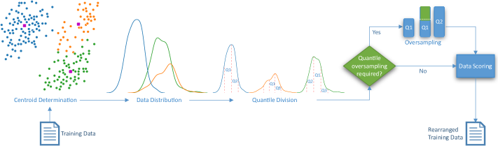
Figure 1: Data Distribution-based Curriculum Learning

II-B Learning style variations

In [27], the Weinshall et al. used transfer learning to implement curriculum learning. They presented an approach where the curriculum was inferred through transfer learning from another network that was pre-trained on another task. A CNN with two architectures trained using curriculum learning was used to evaluate the proposed method on the CIFAR-100 and STL-10 datasets. Experiment results from their work concluded that with curriculum learning the convergence is faster during the beginning of training and improved generalisation is achieved when more difficult tasks are used.

Hacohen et al. applied curriculum learning to the training of deep networks [28]. They used transfer learning and bootstrapping as two different techniques for the easy to hard process which they termed the scoring function. With transfer learning, a ‘teacher’ network was trained on a large dataset and its prediction performance was used as the scoring function. In bootstrapping, a network was trained without a curriculum and its performance on the training data defined the scoring function. Then, the network was retrained from scratch using curriculum learning. For the pacing function, three approaches were used with all pacing functions having comparable performance based on experiments done by the authors. Experiments done on 6 test cases showed that using a curriculum provided high accuracy and better convergence with the amount of improvement ranging from small to large depending on the test case.

Huang et al. [23] propose a different approach to curriculum learning in the area of face recognition. Instead of using a traditional curriculum created by fixed ordering of samples with increasing difficulty, the authors introduce a loss function which incorporates adaptive curriculum learning. During the training process, samples are randomly selected for each mini-batch and the curriculum is created adaptively from the selected samples. Furthermore, the definition of hard samples is dynamic with a sample classified as hard during the start of training becoming easy towards the end. Overall, the loss function emphasizes easy samples at the start and hard samples later. The authors conducted experiments on benchmark data achieving improved performance over other methods.

Recent research has looked at improving the general curriculum learning process. Zhou et al. presented a curriculum learning method known as dynamics-optimized curriculum learning (DoCL) [22]. DoCL selected training samples at each step using weighted sampling based on the scores. The authors conducted experiments on more than 9 datasets achieving results that significantly improved the performance and efficiency compared to existing curriculum learning methods.

II-C Data density based curriculum learning

Our review of literature for curriculum learning has found few papers that utilise the density of the data. These works are presented in this section and our work on DDCL adds to this field of research.

Applying curriculum learning to large data sets has shown promising results. Researchers in [21] presented a method for training deep neural networks on large-scale weakly-supervised web images. Their training strategy utilised curriculum learning to effectively handle the large amount of noisy labels and data imbalance during the training process. They proposed a curriculum created by measuring the complexity of data using the density of its data. Experiments using the proposed training strategy resulted in state-of-the-art performance on benchmark data sets that included Webvision, ImageNet, Clothing-1M and Food-101.

Choi et al. [26] presented another method of using the density of data to generate the curriculum. Their method applied clustering on the data where higher density samples were considered simple and lower density samples were considered as complex. The proposed method was robust against false pseudo-labelled samples due to the use of a pseudo-labelling curriculum. They achieved state-of-the-art classification results on three benchmark datasets.

Curriculum learning has been applied to imbalanced data classification as well. Dynamic Curriculum Learning (DCL) proposed by Wang et.al [25] addressed the problem of requiring prior knowledge to train a system when using conventional techniques. DCL used a two-level curriculum scheduler made up of a sampling scheduler and a loss scheduler. The sampling scheduler found the best samples in a batch to train the model by dynamically managing the target data distributions from imbalanced to balanced and from easy to hard. The loss scheduler controlled the learning weights between classification loss and metric learning loss. Experiments achieved state-of-the-art performance on the CelebA face attribute dataset and the RAP pedestrian attribute dataset.

// Variables:

// Classes: $S$

// Data size: $N$

// $N_{s}$ - data set for class $s$

// $|N_{s}|$ - data size (cardinality)

// $h$ - bandwidth

1 foreach $s\in S$ do

2       ${O_{s}}=\sum_{n=0}^{|N_{s}|}\min_{\mu_{s}\in S}(\parallel x_{n}-\mu_{s}\parallel^{2})$

3       $s=s\cup O_{s}$

4       $E_{s}=\varnothing$

5       foreach $x\in s$ do

6             $E_{s}=E_{s}\>\cup\parallel{O_{s}-x}\parallel$

7            

8       end foreach

9      $D_{s}=\frac{1}{|N_{s}|h}\sum_{i=1}^{|N_{s}|}K(\frac{y-\hat{E}_{i}}{h})$

10       for $q\in Q^{s}$ do

11             if $|q|<3$ then

12                   $q=SMOTE(q)$

13             end if

14            

15       end for

16      if Scoring type $\leftarrow$ “Density” then

17            go to Algorithm 2

18       else if Scoring type $\leftarrow$ “Point” then

19            go to Algorithm 3

20       end if

      Result: $T\leftarrow R_{s}$

21      

22 end foreach

Algorithm 1 DDCL algorithm

III Proposed Curriculum Learning Approach

The curriculum learning approach proposed in this paper is based on the data distribution of a dataset. This is referred to as Data Distribution-based Curriculum Learning (DDCL) and involves multiple steps as visualised through Figure 1. It begins with dividing the data into groups based on their target classes. Then, the centroids for each group is calculated (Centroid Determination) and used to compute the Euclidean distance between each sample and its centroid. The data distribution for every class is determined next and utilised to divide the data for individual classes into quantiles (Q1, Q2, Q3). After quantile division, oversampling is optionally performed on quantiles where the number samples may be highly imbalanced compared to other quantiles. Lastly, the data is scored with either density or point scoring and rearranged for use in training.

The DDCL process is further detailed in Algorithm 1. In the first step of DDCL, the training data samples are grouped according to their classes ($S$) with the number of groups being equal to the number of unique classes in the data. Next, the grouped training data is used to calculate the centroids ($O_{s}$) for each class by performing clustering on each data group. Then, the centroids are used to compute the Euclidean distance from the relevant centroid ($E_{s}$) for each data sample ($x$). The third step determines the data distribution for a class ($D_{s}$) by plotting the normalised values of the Euclidean distances. Once the distribution of the training data is known, the data samples are divided into quantiles ($Q^{s}$). Each quantile ($q$) is then examined for the number of samples and the quantiles with the lowest number of samples are oversampled using SMOTE [33] if there are sufficient samples. SMOTE creates synthetic samples using the original data and different variants of it have been developed [34] since the initial method was proposed. The initial method of SMOTE is used in our proposed approach to address the potential lack of samples in a given quantile. Otherwise, no oversampling is applied due to insufficient samples. After the samples are divided into quantiles and optionally oversampled, each data sample is scored using either density or point scoring and rearranged accordingly ($R_{s}$). Finally, the rearranged training data ($T$) is ready to be passed to one of the learning methods for training and evaluation.

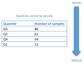
(a) Density scoring

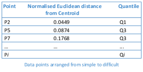
(b) Point scoring

Figure 2: DDCL scoring methods

DDCL consists of two types of scoring methods: a sample density based method and a Euclidean distance based method. These are referred to as DDCL (Density) and DDCL (Point) respectively and are detailed in the following sections.

III-A Density based DDCL

Figure 2(a) illustrates the DDCL (Density) process where the scoring is applied to the quantiles based on the number of samples in the quantile. Quantiles with the greatest number of samples (Q3 - 86) are given a higher score while quantiles with the least number of samples (Q1 - 12) are given a lower score. Higher scores are considered simple while lower scores are considered difficult. This results in a final quantile order sorted from the highest to lowest density thus defining the curriculum to be used during training.

1$C_{s}=\varnothing$

2 foreach $q\in Q^{s}$ do

3       $C_{s}=C_{s}\cup|q|$

4 end foreach

5$R_{s}\leftarrow sort(\forall\>C_{s}|s\in S)$

return $R_{s}$

Algorithm 2 DDCL Density

Algorithm 2 provides details of the DDCL (Density) scoring process. It shows that the process starts with determining the density of each quantile by taking their cardinality, $|q|$. Once the densities for all quantiles ($C_{s}$) are known, the training data is sorted according to their quantile’s density from highest to lowest. Finally, the rearranged data, $R_{s}$, is ready for use in training.

III-B Point based DDCL

On the other hand, Figure 2(b) illustrates how DDCL (Point) assigns a score to the individual data samples in the dataset by utilising their normalised Euclidean distance from centroid rather than examining quantiles. In this scoring method, data samples with the shorter Euclidean distances (P2, P5) are given the highest scores while samples with the longer Euclidean distances (P7, Pi) are assigned the lowest scores. As with DDCL (Density), higher scores in this point scoring method are considered simple while lower scores are considered difficult. Using DDCL (Point) results in a curriculum where the training samples are ordered based on their individual characteristic rather than as a group.

1$R_{s}\leftarrow sort(\forall\>\hat{E_{s}}|s\in S)$

return $R_{s}$

Algorithm 3 DDCL Point

Algorithm 3 explains the DDCL (Point) scoring method and it shows that the data samples are sorted using the normalised Euclidean distance from centroid, $\hat{E_{s}}$. The sorting is done from the shortest distance to the longest regardless of which quantile a sample is assigned to. For example, consider a dataset with four quantiles with each quantile having at least five data samples. The first sample with the lowest $\hat{E_{s}}$ value may belong to quantile 1. Then, the sample with the second lowest $\hat{E_{s}}$ could come from quantile 4. The third lowest $\hat{E_{s}}$ value can be a sample from quantile 2. Next, the fourth lowest $\hat{E_{s}}$ may come from a sample in quantile 3. This method of sorting then repeats until $\hat{E_{s}}$ values from all data samples are accounted for with the resulting order of quantiles and samples ($R_{s}$) becoming randomised in contrast to DDCL (Density).

IV Experiments

DDCL is evaluated by performing classification tasks on 7 datasets obtained from the UCI Machine Learning Repository [35]. Table I lists the datasets used for the experiments. Three types of classifiers are used for evaluating DDCL; neural network, SVM and random forest.

[b] Dataset Data Instances Attributes Class Type Breast Cancer Diagnostic 569 31 Binary Cancer 457 9 Binary Haberman 306 3 Binary Liver Disorder 346 6 Binary Pima Indians Diabetes 768 8 Binary New-Thyroid 215 5 Multi-class Diabetes 130¹ 86556 46 Multi-class

TABLE I: Datasets used for evaluating DDCL.

• Preprocessed version found in [36].

The neural network architecture used for evaluating DDCL consists of one input layer, a variable number of hidden layers and one output layer. The size of the input layer is equal to the number of attributes in the dataset and varies depending on the selected dataset. Similarly, the number of hidden layers changes based on the dataset and is a hyperparameter that can be tuned. Bayesian optimisation is used on the model to tune the hidden layer values. Finally, the size of the output layer can be configured for binary or multi-class classification. The SVM classifier for evaluating DDCL uses a C value of 1.0 with a RBF kernel. The gamma ($\gamma$) value of the RBF kernel scales according to the dataset used. A RBF kernel is chosen due to its good generalisation ability and robustness to input noise. The random forest classifier in our evaluation of DDCL uses 100 estimators and a value of 2 features for splitting a node.

During the neural network experiments, the selected dataset is split into training, validation and testing subsets. 20% of the data is used for validation, 10% for testing and the remainder for training. The neural network model is then trained on the training subset for 200 epochs and tested on the testing subset. Likewise in the SVM and random forest experiments, the selected dataset is split into training and testing subsets with 70% and 30% of the data being used respectively. The SVM and random forest classifiers are trained using the training subset of the data and tested on the testing subset.

For each dataset and classifier, 30 experiments runs are performed using three test scenarios: No Curriculum, DDCL (Density) and DDCL (Point). The first No Curriculum test scenario takes the input data and uses it to train a neural network, SVM and random forest classifier without altering the order of the training data. After training, classification experiments are conducted on the testing subset of data. In the second DDCL (Density) test scenario, the input data is processed using the steps outlined in the DDCL method and scored by density. Classification is then performed on the testing subset as stated earlier. The DDCL (Point) test scenario processes the input data through DDCL with the point scoring approach being used for the scoring step. Experiments for classification are likewise performed on the testing subset.

TABLE II: Neural Network classification results.

Dataset	Test Scenario	Worst %	Best %	Average $\pm$Std. deviation
Breast Cancer Diagnostic	No Curriculum	91.304	100.000	96.232 $\pm$2.442
	DDCL (Density)	89.130	100.000	96.594 $\pm$2.673
	DDCL (Point)	86.957	100.000	97.319 $\pm$2.953
Cancer	No Curriculum	86.486	100.000	94.955 $\pm$3.993
	DDCL (Density)	91.667	100.000	96.852 $\pm$2.658
	DDCL (Point)	86.111	100.000	96.574 $\pm$3.100
Haberman	No Curriculum	45.833	79.167	65.833 $\pm$8.898
	DDCL (Density)	50.000	87.500	69.167 $\pm$10.353
	DDCL (Point)	41.667	87.500	67.222 $\pm$9.424
Liver Disorder	No Curriculum	57.143	85.714	69.048 $\pm$6.477
	DDCL (Density)	46.429	85.714	68.214 $\pm$9.052
	DDCL (Point)	57.143	82.143	69.524 $\pm$6.098
Pima Indians Diabetes	No Curriculum	54.098	86.885	71.803 $\pm$6.658
	DDCL (Density)	55.738	85.246	72.732 $\pm$5.933
	DDCL (Point)	57.377	80.328	71.803 $\pm$5.460
New-Thyroid	No Curriculum	82.353	100.000	93.137 $\pm$5.280
	DDCL (Density)	82.353	100.000	95.490 $\pm$5.409
	DDCL (Point)	82.353	100.000	94.118 $\pm$5.683
Diabetes 130	No Curriculum	53.235	54.694	54.029 $\pm$0.518
	DDCL (Density)	56.148	56.798	56.579 $\pm$0.246
	DDCL (Point)	54.400	56.278	55.139 $\pm$0.696

TABLE III: SVM classification results.

Dataset	Test Scenario	Worst %	Best %	Average $\pm$Std. deviation
Breast Cancer Diagnostic	No Curriculum	94.737	99.415	97.700 $\pm$1.188
	DDCL (Density)	95.322	99.415	97.758 $\pm$1.025
	DDCL (Point)	94.737	99.415	97.719 $\pm$1.239
Cancer	No Curriculum	94.928	99.275	96.715 $\pm$1.134
	DDCL (Density)	94.118	99.265	96.985 $\pm$1.145
	DDCL (Point)	92.647	99.265	96.225 $\pm$1.562
Haberman	No Curriculum	65.217	78.261	72.609 $\pm$4.051
	DDCL (Density)	65.217	83.696	73.841 $\pm$4.836
	DDCL (Point)	67.391	79.348	73.080 $\pm$3.329
Liver Disorder	No Curriculum	44.231	76.923	63.750 $\pm$7.264
	DDCL (Density)	49.038	75.000	66.699 $\pm$5.515
	DDCL (Point)	55.769	75.962	68.558 $\pm$4.783
Pima Indians Diabetes	No Curriculum	71.429	80.519	76.046 $\pm$2.500
	DDCL (Density)	70.996	82.251	77.128 $\pm$2.991
	DDCL (Point)	72.294	82.684	76.508 $\pm$2.514
New-Thyroid	No Curriculum	92.308	100.000	97.128 $\pm$2.472
	DDCL (Density)	92.308	100.000	97.282 $\pm$1.892
	DDCL (Point)	92.308	100.000	96.872 $\pm$1.563
Diabetes 130	No Curriculum	64.285	65.487	64.948 $\pm$0.302
	DDCL (Density)	64.220	65.457	64.977 $\pm$0.298
	DDCL (Point)	64.301	65.469	65.052 $\pm$0.266

TABLE IV: Random Forest classification results.

Dataset	Test Scenario	Worst %	Best %	Average $\pm$Std. deviation
Breast Cancer Diagnostic	No Curriculum	94.152	98.246	95.945 $\pm$1.034
	DDCL (Density)	92.398	98.246	95.653 $\pm$1.581
	DDCL (Point)	91.228	98.246	95.945 $\pm$1.517
Cancer	No Curriculum	92.754	100.000	97.150 $\pm$1.374
	DDCL (Density)	94.853	100.000	96.691 $\pm$1.298
	DDCL (Point)	94.118	100.000	97.206 $\pm$1.361
Haberman	No Curriculum	58.696	76.087	68.261 $\pm$4.100
	DDCL (Density)	65.217	79.348	70.145 $\pm$3.825
	DDCL (Point)	57.609	77.174	69.746 $\pm$4.367
Liver Disorder	No Curriculum	59.615	78.846	70.417 $\pm$5.104
	DDCL (Density)	67.308	77.885	72.917 $\pm$2.709
	DDCL (Point)	60.577	78.846	70.064 $\pm$4.077
Pima Indians Diabetes	No Curriculum	71.861	79.654	75.483 $\pm$1.985
	DDCL (Density)	70.996	80.087	75.339 $\pm$2.200
	DDCL (Point)	65.368	81.818	76.003 $\pm$3.461
New-Thyroid	No Curriculum	95.385	100.000	97.949 $\pm$1.214
	DDCL (Density)	92.308	100.000	98.000 $\pm$1.911
	DDCL (Point)	95.385	100.000	97.897 $\pm$1.512
Diabetes 130	No Curriculum	65.830	66.658	66.218 $\pm$0.228
	DDCL (Density)	65.626	66.948	66.242 $\pm$0.309
	DDCL (Point)	65.542	66.805	66.199 $\pm$0.293

The results of all three test scenarios using neural networks, SVM and random forest classifiers are given in Table III, Table III and Table IV respectively.

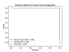
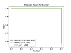
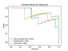
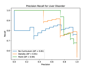
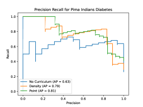
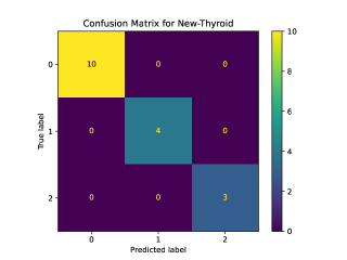
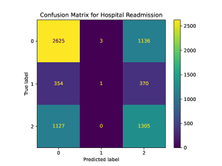
Figure 3: Precision-Recall curves for binary classification datasets and confusion matrix for multi-class datasets.

V Discussion

Observations on the learning methods show that the classification performance across the datasets is always increased whenever DDCL is applied. This is true regardless of the learning method used as shown in Table III, Table III and Table IV.

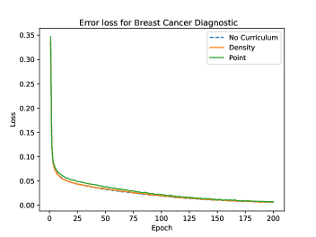
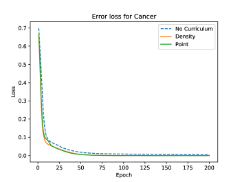
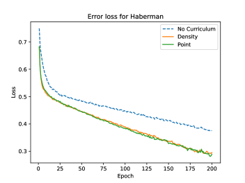
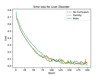
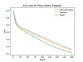
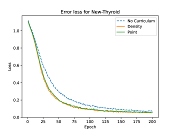
Figure 4: Error loss per epoch for neural network classifier.

Using the neural network classifier provides the highest best results for the Haberman, Liver Disorder and Pima Indians Diabetes datasets while the SVM method achieves the highest average results on the Breast Cancer Diagnostic, Haberman and Pima Indians Diabetes data. The random forest based classifier yields the highest average result for the Cancer, Liver Disorder, New-Thyroid and Diabetes 130 datasets. Notably, using DDCL with SVM and random forest approaches results in significant increases in average accuracy for Haberman and Liver Disorder data respectively compared to other learning methods. Figure 3 shows the precision-recall curves for the best result of each binary classification dataset when using the neural network method. For multi-class data, the confusion matrix is provided in place of the precision-recall curves.

The highest average result for Breast Cancer Diagnostic was achieved using SVM with density-based DDCL while the largest improvement (1.087%) was using the neural network with point-based DDCL. For the Cancer dataset, using random forest with point-based DDCL provided the highest average accuracy and using the neural network with density-based DDCL gave the most improved accuracy (1.897%). Using SVM with density-based DDCL resulted in the highest average accuracy when evaluated on the Haberman data. The largest improvement for this dataset (3.334%) was observed when using density-based DDCL with the neural network. The highest average result for Liver Disorder was achieved using random forest with density-based DDCL while the SVM gave the largest average accuracy improvement at 4.808%. For the Pima Indians Diabetes dataset, the highest average accuracy was obtained using SVM with density-based DDCL which was also the most improved accuracy (1.082%).

In multi-class classification, using random forest with density-based DDCL resulted in the highest average accuracy on the New-Thyroid data and the largest improvement for this dataset came from density-based DDCL applied to the neural network. For the Diabetes 130 data, density-based DDCL with random forest provided the highest average accuracy while the largest improvement in accuracy (2.550%) was obtained through the neural network classifier utilising density-based DDCL.

The experiment results demonstrate that using DDCL to order the training data for a given learning method leads to improvements in classification accuracy. This can be seen in the performance of all datasets tested with either the density or point-based DDCL approach having increased performance compared to the no curriculum approach. Figure 4 shows the error loss per epoch plots when using the neural network classifier for each dataset except for Diabetes 130 which is excluded since its average accuracy is not significant [36]. The plots show that using DDCL leads to better reduction in the error loss.

In addition, using DDCL to order the training data results in faster convergence. We arrived at this conclusion by examining the error loss for the first five epochs of each dataset using batch gradient descent. Figure 5 shows the error loss plots for each dataset. It can be seen that the overall losses for DDCL (Density) and DDCL (Point) are reduced faster compared to the no curriculum approach thus leading to faster convergence towards the minimum. This is consistent with the findings of the error loss against epoch plots in Figure 4 where the error loss towards the end is lower for DDCL (Density) and DDCL (Point).

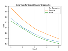
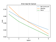
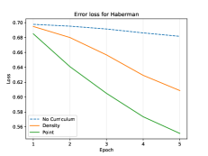
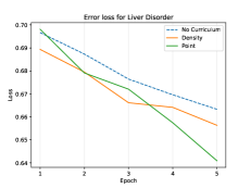
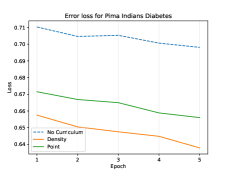
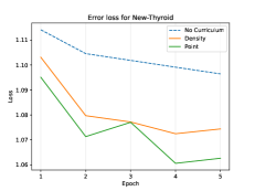
Figure 5: Error loss per epoch with batch gradient descent for neural network classifier.

VI Conclusion

This paper proposed a curriculum learning approach known as Data Distribution-based Curriculum Learning (DDCL). It used the data distribution of a dataset to build a curriculum based on the order of samples. Two types of scoring methods known as DDCL (Density) and DDCL (Point) were used to score samples thus determining their training order. DDCL (Density) used the sample density to assign scores while DDCL (Point) utilised the Euclidean distance for scoring.

Experiments were conducted on multiple datasets using a neural network, SVM and random forest classifier to evaluate DDCL. Results showed that while performance varied across the datasets depending on the classifier used, the application of DDCL resulted in significant increases in the average accuracy for most datasets compared to not using any curriculum. Furthermore, analysis of the error losses for five training epochs using batch gradient descent reveals that convergence is faster when using DDCL with either of the scoring methods over the no curriculum method.

The current DDCL approach uses only two types of scoring methods and is limited to using a single scoring method at a time. Moreover, the proposed approach uses a fixed curriculum that is pre-determined before the start of training and does not take into account the current training progress.

Future work will explore the creation of additional scoring methods to determine their impact on the training performance and investigate the application of ensemble learning using each scoring method. In addition, self-paced learning concepts will be incorporated into DDCL in order to dynamically determine the curriculum based on feedback from the learner. The proposed approach can also be adapted to image and text processing applications.

References

- [1] A. E. Maxwell, T. A. Warner, and F. Fang, “Implementation of machine-learning classification in remote sensing: an applied review,” International Journal of Remote Sensing, vol. 39, no. 9, pp. 2784–2817, May 2018. [Online]. Available: https://doi.org/10.1080/01431161.2018.1433343
- [2] A. Dongare, R. Kharde, A. D. Kachare et al., “Introduction to artificial neural network,” International Journal of Engineering and Innovative Technology (IJEIT), vol. 2, no. 1, pp. 189–194, 2012.
- [3] O. Chapelle, P. Haffner, and V. Vapnik, “Support vector machines for histogram-based image classification,” IEEE Transactions on Neural Networks, vol. 10, no. 5, pp. 1055–1064, Sep. 1999, conference Name: IEEE Transactions on Neural Networks.
- [4] L. Breiman, “Random Forests,” Machine Learning, vol. 45, no. 1, pp. 5–32, Oct. 2001. [Online]. Available: https://doi.org/10.1023/A:1010933404324
- [5] V. Gudivada, A. Apon, and J. Ding, “Data Quality Considerations for Big Data and Machine Learning: Going Beyond Data Cleaning and Transformations,” International Journal on Advances in Software, vol. 10, pp. 1–20, 07 2017.
- [6] H. Finch, “Distribution of Variables by Method of Outlier Detection,” Frontiers in Psychology, vol. 3, p. 211, 2012. [Online]. Available: https://www.frontiersin.org/article/10.3389/fpsyg.2012.00211
- [7] I. Taleb, M. A. Serhani, and R. Dssouli, “Big Data Quality: A Survey,” in 2018 IEEE International Congress on Big Data (BigData Congress), Jul. 2018, pp. 166–173.
- [8] D. Weiss, C. Alberti, M. Collins, and S. Petrov, “Structured training for neural network transition-based parsing,” CoRR, vol. abs/1506.06158, 2015. [Online]. Available: http://arxiv.org/abs/1506.06158
- [9] M. Andrychowicz, M. Denil, S. Gómez, M. W. Hoffman, D. Pfau, T. Schaul, B. Shillingford, and N. de Freitas, “Learning to learn by gradient descent by gradient descent,” in Advances in Neural Information Processing Systems, D. Lee, M. Sugiyama, U. Luxburg, I. Guyon, and R. Garnett, Eds., vol. 29. Curran Associates, Inc., 2016. [Online]. Available: https://proceedings.neurips.cc/paper/2016/file/fb87582825f9d28a8d42c5e5e5e8b23d-Paper.pdf
- [10] Y. Zhang, H. Tang, and K. Jia, “Fine-Grained Visual Categorization using Meta-Learning Optimization with Sample Selection of Auxiliary Data,” in Computer Vision – ECCV 2018. Cham: Springer International Publishing, 2018, pp. 241–256.
- [11] A. Sharma, “Guided stochastic gradient descent algorithm for inconsistent datasets,” Applied Soft Computing, vol. 73, pp. 1068–1080, 2018. [Online]. Available: https://www.sciencedirect.com/science/article/pii/S156849461830557X
- [12] S. Ruder, “An overview of gradient descent optimization algorithms,” CoRR, vol. abs/1609.04747, 2016. [Online]. Available: http://arxiv.org/abs/1609.04747
- [13] J. Wainer and P. Fonseca, “How to tune the RBF SVM hyperparameters? An empirical evaluation of 18 search algorithms,” Artificial Intelligence Review, vol. 54, no. 6, pp. 4771–4797, Aug. 2021. [Online]. Available: https://doi.org/10.1007/s10462-021-10011-5
- [14] P. Probst, M. N. Wright, and A.-L. Boulesteix, “Hyperparameters and tuning strategies for random forest,” WIREs Data Mining and Knowledge Discovery, vol. 9, no. 3, p. e1301, 2019, _eprint: https://onlinelibrary.wiley.com/doi/pdf/10.1002/widm.1301. [Online]. Available: https://onlinelibrary.wiley.com/doi/abs/10.1002/widm.1301
- [15] N. G. Gyori, M. Palombo, C. A. Clark, H. Zhang, and D. C. Alexander, “Training data distribution significantly impacts the estimation of tissue microstructure with machine learning,” Magnetic Resonance in Medicine, vol. 87, no. 2, pp. 932–947, 2022, _eprint: https://onlinelibrary.wiley.com/doi/pdf/10.1002/mrm.29014. [Online]. Available: https://onlinelibrary.wiley.com/doi/abs/10.1002/mrm.29014
- [16] L. A. Jeni, J. F. Cohn, and F. De La Torre, “Facing Imbalanced Data–Recommendations for the Use of Performance Metrics,” in 2013 Humaine Association Conference on Affective Computing and Intelligent Interaction, Sep. 2013, pp. 245–251, iSSN: 2156-8111.
- [17] X. Ma, F. Liu, S. Ge, and X. Wu, “Competence-based Multimodal Curriculum Learning for Medical Report Generation,” Oct. 2022, arXiv:2206.14579 [cs]. [Online]. Available: http://arxiv.org/abs/2206.14579
- [18] Y. Bengio, J. Louradour, R. Collobert, and J. Weston, “Curriculum learning,” in Proceedings of the 26th annual international conference on machine learning, 2009, pp. 41–48.
- [19] O. Erstad and J. Voogt, “The Twenty-First Century Curriculum: Issues and Challenges,” 978-3-319-71053-2, pp. 19–36, 2018, accepted: 2020-01-03T19:44:53Z Publisher: Springer. [Online]. Available: https://www.duo.uio.no/handle/10852/71882
- [20] K. A. Krueger and P. Dayan, “Flexible shaping: How learning in small steps helps,” Cognition, vol. 110, no. 3, pp. 380–394, 2009, number: 3. [Online]. Available: https://www.sciencedirect.com/science/article/pii/S0010027708002850
- [21] S. Guo, W. Huang, H. Zhang, C. Zhuang, D. Dong, M. R. Scott, and D. Huang, “Curriculumnet: Weakly supervised learning from large-scale web images,” in Proceedings of the European Conference on Computer Vision (ECCV), 2018, pp. 135–150.
- [22] T. Zhou, S. Wang, and J. Bilmes, “Curriculum Learning by Optimizing Learning Dynamics,” in Proceedings of The 24th International Conference on Artificial Intelligence and Statistics. PMLR, Mar. 2021, pp. 433–441, iSSN: 2640-3498. [Online]. Available: https://proceedings.mlr.press/v130/zhou21a.html
- [23] Y. Huang, Y. Wang, Y. Tai, X. Liu, P. Shen, S. Li, J. Li, and F. Huang, “CurricularFace: Adaptive Curriculum Learning Loss for Deep Face Recognition,” in Proceedings of the IEEE/CVF Conference on Computer Vision and Pattern Recognition (CVPR), 2020, pp. 5901–5910.
- [24] N. Sarafianos, T. Giannakopoulos, C. Nikou, and I. A. Kakadiaris, “Curriculum learning of visual attribute clusters for multi-task classification,” Pattern Recognition, vol. 80, pp. 94–108, 2018. [Online]. Available: https://www.sciencedirect.com/science/article/pii/S0031320318300840
- [25] Y. Wang, W. Gan, J. Yang, W. Wu, and J. Yan, “Dynamic curriculum learning for imbalanced data classification,” in 2019 IEEE/CVF International Conference on Computer Vision (ICCV), 2019, pp. 5016–5025.
- [26] J. Choi, M. Jeong, T. Kim, and C. Kim, “Pseudo-Labeling Curriculum for Unsupervised Domain Adaptation,” Aug. 2019, arXiv:1908.00262 [cs]. [Online]. Available: http://arxiv.org/abs/1908.00262
- [27] D. Weinshall, G. Cohen, and D. Amir, “Curriculum learning by transfer learning: Theory and experiments with deep networks,” in International Conference on Machine Learning. PMLR, 2018, pp. 5238–5246.
- [28] G. Hacohen and D. Weinshall, “On the power of curriculum learning in training deep networks,” in International Conference on Machine Learning. PMLR, 2019, pp. 2535–2544.
- [29] S. Narvekar, B. Peng, M. Leonetti, J. Sinapov, M. E. Taylor, and P. Stone, “Curriculum learning for reinforcement learning domains: A framework and survey,” arXiv preprint arXiv:2003.04960, 2020.
- [30] B. Tidd, N. Hudson, and A. Cosgun, “Guided Curriculum Learning for Walking Over Complex Terrain,” Feb. 2021, arXiv:2010.03848 [cs]. [Online]. Available: http://arxiv.org/abs/2010.03848
- [31] M. Kumar, B. Packer, and D. Koller, “Self-Paced Learning for Latent Variable Models,” in Advances in Neural Information Processing Systems, vol. 23. Curran Associates, Inc., 2010. [Online]. Available: https://proceedings.neurips.cc/paper/2010/hash/e57c6b956a6521b28495f2886ca0977a-Abstract.html
- [32] L. Jiang, D. Meng, Q. Zhao, S. Shan, and A. G. Hauptmann, “Self-Paced Curriculum Learning,” in Proceedings of the Twenty-Ninth AAAI Conference on Artificial Intelligence, ser. AAAI’15, 2015, pp. 2694–2700, event-place: Austin, Texas.
- [33] N. V. Chawla, K. W. Bowyer, L. O. Hall, and W. P. Kegelmeyer, “SMOTE: Synthetic Minority Over-sampling Technique,” Journal of Artificial Intelligence Research, vol. 16, pp. 321–357, Jun. 2002. [Online]. Available: https://www.jair.org/index.php/jair/article/view/10302
- [34] A. Sharma, P. K. Singh, and R. Chandra, “SMOTified-GAN for Class Imbalanced Pattern Classification Problems,” IEEE Access, vol. 10, pp. 30 655–30 665, 2022, conference Name: IEEE Access.
- [35] D. Dua and C. Graff, “UCI machine learning repository,” 2017. [Online]. Available: http://archive.ics.uci.edu/ml
- [36] Shane, “Readmission Prediction,” Jun. 2022, original-date: 2018-12-23T14:42:57Z. [Online]. Available: https://github.com/freesinger/readmission_prediction