Self-Consistent Conformal Prediction

Abstract

In decision-making guided by machine learning, decision-makers often take identical actions in contexts with identical predicted outcomes. Conformal prediction helps decision-makers quantify outcome uncertainty for actions, allowing for better risk management. Inspired by this perspective, we introduce self-consistent conformal prediction, which yields both Venn-Abers calibrated predictions and conformal prediction intervals that are valid conditional on actions prompted by model predictions. Our procedure can be applied post-hoc to any black-box predictor to provide rigorous, action-specific decision-making guarantees. Numerical experiments show our approach strikes a balance between interval efficiency and conditional validity.

1 Introduction

Incorporating machine learning into decision-making processes has shown significant promise in improving post-decision outcomes, such as better medical treatments, increased operational efficiency, and reduced costs (Lee et al., 2015; Kang et al., 2015; Bhardwaj et al., 2017; Awaysheh et al., 2019; Marr, 2019; Sircar et al., 2021). Particularly in safety-critical sectors, such as healthcare, it is important to ensure that decisions inferred from predictions made by machine learning models are reliable, under minimal assumptions (Mandinach et al., 2006; Veale et al., 2018; Char et al., 2018; Quest et al., 2018). As a response, there has been growing interest in predictive inference approaches to decision-making, allowing for rigorous risk assessment by quantifying deviations of outcomes from model predictions.

Conformal prediction (CP) is a popular, model-agnostic, and distribution-free framework for predictive inference, which can be applied post-hoc to any prediction pipeline (Vovk et al., 2005; Shafer & Vovk, 2008; Balasubramanian et al., 2014; Lei et al., 2018). Given a prediction issued by a black-box model, CP outputs a prediction interval that is guaranteed to contain the unobserved outcome with a user-specified probability (Lei et al., 2018). However, a limitation of CP is that the prediction intervals provide valid coverage only marginally, averaged across all possible contexts – where ‘context’ refers to the information available for decision-making. Thus, for a specific context, CP intervals may not accurately capture the true outcome variability, leading to unreliable and potentially harmful decision-making (van Calster et al., 2019; Lloyd-Jones et al., 2019).

The construction of informative prediction intervals that provide valid conditional coverage, within a specific context, is generally unachievable without additional distributional assumptions (Vovk, 2012; Barber et al., 2021). However, it is possible to construct prediction intervals that achieve weaker forms of conditional validity. For example, given a finite set of subgroups, Mondrian CP (Vovk et al., 2005; Boström et al., 2021) provides intervals that maintain valid coverage within each subgroup. Generalizing Mondrian CP, Gibbs et al. 2023 introduced a regularized conditional CP framework for constructing prediction intervals that achieve approximately valid coverage uniformly over a potentially infinite-dimensional class of distribution shifts. Their approach provides a means to trade-off the efficiency (i.e., width) of CP intervals and the degree of conditional coverage achieved, interpolating between marginal and conditional guarantees. However, they demonstrate the existence of a “curse of dimensionality”: as the dimension of the context increases, smaller classes of distribution shifts must be considered to retain the same level of precision. Thus, especially in data-rich contexts such as those in medical applications, prediction intervals with meaningful context-specific coverage guarantees may be too wide to effectively inform decision-making.

Motivation. In this work, we consider a more feasible and practical notion of conditional coverage, motivated by how CP may be used in real-world decision-making. In a decision-making process guided by a machine learning model, a decision-maker typically takes identical actions for contexts with identical predicted outcomes. Predictive inference methods such as CP provide prediction intervals that assist decision-makers in focusing on contexts with sufficient signal — evidenced by the interval’s width — thus reducing the risk of harmful actions. Since both point and interval predictions play a role in decision-making, it is important that (i) point predictions associated with the same action are well-calibrated, neither overestimating nor underestimating outcomes; and (ii) prediction intervals are valid conditional on the actions prompted by point predictions.

Contributions. We propose Self-Consistent Conformal Prediction (SC-CP), which simultaneously provides Venn-Abers calibrated predictions (Vovk & Petej, 2012) and conformal prediction intervals that, in finite samples, are valid conditionally on model predictions and, thereby, on any actions inferred from them. By aiming for validity conditional on the model output, SC-CP provides meaningful action-specific decision-making guarantees, while avoiding the curse of dimensionality inherent in context-specific validity.

2 Preliminaries

2.1 Notation

We consider a standard regression setup in which the input $X\in\mathcal{X}\subset\mathbb{R}^{d}$ corresponds to contextual information available for decision-making, and the output $Y\in\mathcal{Y}\subset\mathbb{R}$ is an outcome of interest. We assume that we have access to a calibration dataset $\mathcal{C}_{n}=\{(X_{i},Y_{i})\}_{i=1}^{n}$ comprising $n$ i.i.d. data points drawn from an unknown distribution $P:=P_{X}P_{Y\mid X}$. We assume access to a black-box predictor $f:\mathcal{X}\mapsto\mathcal{Y}$, obtained by training an ML model on a dataset that is independent of $\mathcal{C}_{n}$. Throughout this paper, we do not make any assumptions on the model $f$ or the distribution $P$.

2.2 Objectives

Let $(X_{n+1},Y_{n+1})$ be a new data point drawn from $P$ independently of the calibration data $\mathcal{C}_{n}$. Our goal is to develop a predictive inference algorithm that constructs a prediction interval $\widehat{C}_{n}(X_{n+1})$ around the point prediction issued by the black-box model, i.e., $f(X_{n+1})$. For this prediction interval to be deemed valid, it should cover the true outcome $Y_{n+1}$ with a probability $1-\alpha$. Conformal prediction (CP) is a method for predictive inference that can be applied in a post-hoc fashion to any black-box model (Vovk et al., 2005). The vanilla CP procedure issues prediction intervals that satisfy the following marginal coverage condition:

$$P(Y_{n+1}\in\widehat{C}_{n}(X_{n+1}))\geq 1-\alpha.$$ (1)

However, marginal coverage might lack utility in decision-making scenarios where decisions are context-dependent. A prediction band $\widehat{C}_{n}(x)$ achieving 95% coverage may exhibit arbitrarily poor coverage for specific contexts $x$, or achieve coverage on predictions that are already less uncertain or less relevant to the decision-maker. Ideally, we would like this coverage condition to hold for each context $x\in\mathcal{X}$, i.e., the conventional notion of “conditional validity” requires

$$P(Y_{n+1}\in\widehat{C}_{n}(X_{n+1})|X_{n+1}=x)\geq 1-\alpha,$$ (2)

for all $x\in\mathcal{X}$. However, previous work has shown that it is impossible to achieve (2) without making further distribution assumptions (Barber et al., 2021). In this paper, we aim for a new notion of coverage that is feasible in finite samples while still addressing decision-making requirements.

Uncertainties in decision-making. In a decision-making process guided by the black-box model $f(\cdot)$, the decision-maker will typically take identical actions for all contexts $x$ sharing the same predicted value $f(x)$, i.e., the action $a\in\mathcal{A}$ associated with each context $x$ is $a(x)=a(f(x))$. For example, if $f(\cdot)$ predicts the future biomarker value in a medical setting, a clinician might use an intervention (e.g., an antibiotic) for patient $x$ to stabilize the biomarker if $f(x)$ falls out of the normal range. The width of the prediction interval, $\widehat{C}_{n}(x)$, serves as an additional signal for decision-making. In the set of patients with the same point prediction $\{x^{\prime}\in\mathcal{X}:\forall f(x^{\prime})=\bar{f}\}$, the intervention may be applied selectively, focusing on contexts where the interval width $\widehat{C}_{n}(\cdot)$ is sufficiently small in order to minimize the risk of over-treatment and unnecessary side effects. Here, both the point and interval predictions play a role in decision-making. A conditionally-valid prediction interval holds little value if the corresponding point prediction is inaccurate, while an accurate point prediction can be unactionable if the associated uncertainty interval is invalid.

Motivated by this perspective, our goal is to develop a variant of the CP procedure with guarantees that are relevant to practical decision-making settings. Since both point and interval estimates contribute to decisions, we consider inference procedures with the following desiderata:

1. Point predictions associated with the same action are well-calibrated.

2. Prediction intervals are valid conditional on the actions prompted by point predictions.

In the medical example mentioned earlier, desideratum (i) implies that point predictions from $f(\cdot)$ should be accurate, on average, for all contexts assigned the same action. For instance, for all patients treated with an antibiotic, the average biomarker for this group should indeed be low. Desideratum (ii) indicates that prediction intervals should be valid within the subset of all contexts receiving the same action. For example, within the set of patients treated with an antibiotic, the intervals should accurately cover their true biomarker ranges. If we assume that the black-box model predictions are sufficient statistics for decisions, i.e., $a(x)=a(f(x))$, it is then sufficient to develop procedures that are conditionally valid with respect to the predictions $f(x)$ rather than the infeasible condition of context-specific validity in (2).

Self-consistency. We formalize desiderata (i) and (ii) using the notion of self-consistency of random variables. For two jointly distributed random vectors $\boldsymbol{X}$ and $\boldsymbol{Y}$, we say that $\boldsymbol{Y}$ is self-consistent for $\boldsymbol{X}$ if $E[\boldsymbol{X}|\boldsymbol{Y}]=\boldsymbol{Y}$ almost surely (Definition 2.1 in Flury & Tarpey 1996). We can rewrite (i) and (ii) in the form of self-consistency properties as follows:

1. Self-Consistent Point Predictions:

   $f(X_{n+1})=\mathbb{E}[Y_{n+1}\mid f(X_{n+1})].$

2. Self-Consistent Prediction Intervals:

   $P(Y_{n+1}\in\widehat{C}_{n}(X_{n+1})|f(X_{n+1}))\geq 1-\alpha.$

The concept of self-consistency traces back to Efron, who introduced it in 1967 to characterize estimators for a distribution function in the context of censored data Efron 1967. Condition (i) states that the (black-box) prediction $f(X_{n+1})$ should be self-consistent for the true outcome $Y_{n+1}$—a condition also known in the literature as “perfect calibration” (Gupta et al., 2020; van der Laan et al., 2023). Condition (ii) presents a more relaxed version of the infeasible coverage condition in (2), requiring the prediction interval for $X_{n+1}$ to provide valid coverage for $Y_{n+1}$ based on the (self-consistent) outcome prediction rather than the context $X_{n+1}$. Throughout the remainder of this paper, we will develop a variant of CP that fulfils both conditions (i) and (ii).

3 Self-Consistent Conformal Prediction

A key advantage of CP is that it can be applied in a post-hoc fashion to any black-box model $f$ without disrupting its point predictions. However, desideratum (i) introduces a self-consistency requirement for the point predictions of $f$, thereby interfering with the underlying model specification. In this section, we introduce a modified version of CP, Self-Consistent CP (SC-CP), that satisfies (i) & (ii) while preserving all the favorable properties of CP, including its finite-sample validity and post-hoc applicability.

3.1 Conformalizing Venn-Abers Predictors

To achieve desiderata (i) and (ii), we propose a predictive inference procedure that combines two post-hoc approaches: Venn-Abers calibration (Vovk & Petej, 2012) and split CP (Li et al., 2018). The key idea behind our method is to first apply a post-hoc calibration step to the point predictions using methods akin to isotonic regression in order to achieve the self-consistency property (i) in finite-sample. Next, we apply split CP within bins of the calibrated point predictions in order to achieve the coverage guarantee in (ii). Before describing our complete procedure in Section 3.2, we provide a brief background on Venn-Abers Predictors.

Venn-Abers Predictors. In this paper, we consider a formulation of Venn-Abers calibration as a generalized form of isotonic calibration (Zadrozny & Elkan, 2002; Niculescu-Mizil & Caruana, 2005; van der Laan et al., 2023). We define a function class $\Theta_{\text{iso}}$ as an isotonic calibrator class if it satisfies the following properties: (a) It consists of univariate regression trees that are monotonically nondecreasing and of finite depth; (b) For all elements $\theta\in\Theta_{\text{iso}}$ and transformations $g:\mathbb{R}\rightarrow\mathbb{R}$, it holds that $g\circ\theta\in\Theta_{\text{iso}}$. Here, we adopt the relaxed definition of a tree as any piecewise constant function, so that Property (a) ensures that elements of $\Theta_{\text{iso}}$ are piecewise constant isotonic functions with finite range. Property (b) ensures invariance under transformations, which guarantees that $\Theta_{\text{iso}}$ remains unchanged when its elements undergo relabeling of their leaves. Notably, the maximal isotonic calibrator class consists of all univariate, piecewise constant isotonic functions of finite range.

Given the isotonic calibrator class $\Theta_{\text{iso}}$ and a calibration dataset $\mathcal{C}_{n}=\{(X_{1},Y_{1}),\dots,(X_{n},Y_{n})\}$, the standard isotonic regression procedure calibrates the initial black-box model $f$ by finding a 1D function from the isotonic calibrator class $\Theta_{\text{iso}}$ so that $\theta\circ f$ best fits the labels in calibration data — the monotonicity constraint provides implicit regularization. In Algorithm 1, we propose a generalization of isotonic calibration where calibration is iteratively applied on imputed labels to produce a prediction set instead of a point prediction. This algorithm can be viewed as the regression counterpart of the original Venn-Abers procedure for probability calibration in the classification setup. As we will show later, the oracle version of this procedure achieves the self-consistency property in (i). SC-CP conformalizes Venn-Abers predictors by applying CP on top of the outputs of Algorithm 1.

3.2 Oracle SC-CP Procedure

Algorithm 1 Venn-Abers Calibration

0:  Calibration data $\mathcal{C}_{n}=\{(X_{1},Y_{1}),\dots,(X_{n},Y_{n})\}$, isotonic calibrator class $\Theta_{\text{iso}}$, black-box model $f$, context $x\in\mathcal{X}$.

1:  for each $y\in\mathcal{Y}$ do

2:    Set augmented dataset $\mathcal{C}_{n}^{(x,y)}:=\mathcal{C}_{n}\cup\{(x,y)\}$;

3:    Apply isotonic calibration to $f$ using $\mathcal{C}_{n}^{(x,y)}$ and $\Theta_{\text{iso}}$:  $\theta_{n}^{(x,y)}:=\operatorname*{argmin}_{\theta\in\Theta_{\text{iso}}}\sum_{i\in\mathcal{C}_{n}^{(x,y)}}\{Y_{i}-\theta\circ f(X_{i})\}^{2}$. $f_{n}^{(x,y)}:=\theta_{n}^{(x,y)}\circ f$.

4:  end for

4:  Venn-Abers prediction $\{f_{n}^{(x,y)}(x):y\in\mathcal{Y}\}$.

To motivate our procedure, we first present an oracle version of our procedure that satisfies desiderata (i) & (ii). Let $\mathcal{C}_{n+1}^{*}=\left\{(X_{i},Y_{i})\right\}_{i=1}^{n+1}$ be an oracle-augmented calibration set obtained by combining observed data $\mathcal{C}_{n}\cup\{X_{n+1}\}$ with the unobserved outcome $Y_{n+1}$. The oracle procedure combines Venn-Abers calibration and CP as follows:

Step 1: Venn-Abers calibration. Given the initial black-box predictive model $f$, calibration data $\mathcal{C}_{n+1}^{*}$, and an isotonic calibrator class $\Theta_{\text{iso}}$, we learn an oracle Venn-Abers predictor $f_{n+1}^{*}:=f_{n}^{(X_{n+1},Y_{n+1})}$ by isotonic calibrating $f$ as in Algorithm 1. From Vovk & Petej 2012, we know that this oracle Venn-Abers predictor is “perfectly calibrated” for $Y_{n+1}$, meaning that its point-prediction satisfies desideratum (i), i.e., $f_{n+1}^{*}(X_{n+1})=\mathbb{E}[Y_{n+1}\mid f_{n+1}^{*}(X_{n+1})]$.

Step 2: Conditionally-valid CP. In this step, we construct a CP interval $C_{n+1}^{*}(X_{n+1})$ centered around $f_{n+1}^{*}(X_{n+1})$. To ensure that it satisfies desideratum (ii), i.e., $C_{n+1}^{*}(X_{n+1})$ is valid conditional on $f_{n+1}^{*}(X_{n+1})$, we adapt the conditionally valid CP framework in Gibbs et al. 2023 to construct a prediction interval that is multi-calibrated against the class of distribution shifts $\left\{\theta\circ f_{n+1}^{*};\ \theta:\mathbb{R}\to\mathbb{R}\right\}$. (Here, we conceptualize the calibration function $\theta$ as a “distribution shift” in line with the covariate shift framing in Sec 1. in Gibbs et al. 2023.) Let $S_{i}:=|Y_{i}-f_{n+1}^{*}(X_{i})|$ for $i\in[n+1]$ be the conformity scores. For a quantile level $\alpha\in(0,1)$, we define the “pinball” quantile loss $\ell_{\alpha}$ as

$$\ell_{\alpha}(y,f(x)):=\begin{cases}\alpha(y-f(x)),&\text{if }y\geq f(x),\\ (1-\alpha)(f(x)-y)&\text{if }y<f(x).\end{cases}$$

The CP interval is then given by $C_{n+1}^{*}(X_{n+1}):=f_{n+1}^{*}(X_{n+1})\pm\rho_{n+1}^{*}(X_{n+1})$, where $\rho_{n+1}^{*}(X_{n+1})$ is an estimate of the $1-\alpha$ quantile of $S_{n+1}$, computed as

$$\rho_{n+1}^{*}\in\operatorname*{argmin}_{\theta\circ f_{n+1}^{*};\theta:\mathbb{R}\to\mathbb{R}}\frac{1}{n+1}\sum_{i=1}^{n+1}\ell_{\alpha}\left(\theta\circ f_{n+1}^{*}(X_{i}),S_{i}\right).$$

It follows from the main results in Gibbs et al. 2023 that $\mathbb{P}(Y_{n+1}\in C_{n+1}^{*}(X_{n+1})\mid f_{n+1}^{*}(X_{n+1}))\geq 1-\alpha$, i.e., the interval $C_{n+1}^{*}(X_{n+1})$ achieves desideratum (ii). At first glance, one might worry that the resulting prediction interval could be excessively wide and variable, possibly due to the overfitting of the unconstrained empirical risk minimizer $\rho_{n+1}^{*}$. However, the optimization problem is intrinsically regularized because the structure of regression trees remains unchanged under composition with univariate transformations. In particular, for each transformation $\theta:\mathbb{R}\rightarrow\mathbb{R}$, the trees $\theta\circ f_{n+1}^{*}$ and $f_{n+1}^{*}$ are equivalent up to relabelling of their leaf values. As a result, $\rho_{n+1}^{*}(X_{n+1})$ can be efficiently computed as the empirical $1-\alpha$ quantile of the conformity scores within the same leaf as $X_{n+1}$, that is, $\{S_{i}^{*}:f_{n+1}^{*}(X_{i})=f_{n+1}^{*}(X_{n+1}),\,i\in[n+1]\}$.

Algorithm 2 Self-Consistent Conformal Prediction

0:  Calibration data $\mathcal{C}_{n}=\{(X_{1},Y_{1}),\dots,(X_{n},Y_{n})\}$, isotonic calibrator class $\Theta_{\text{iso}}$, black-box model $f$, context $x\in\mathcal{X}$, and miscoverage level $\alpha\in(0,1)$

1:  Obtain Venn-Abers prediction $\{f_{n}^{(x,y)}(x):y\in\mathcal{Y}\}$ by applying Algorithm 1 with $\mathcal{C}_{n}$, $\Theta_{\text{iso}}$, $f$, and $x$;

2:  for each $y\in\mathcal{Y}$ do

3:    Set Venn-Abers conformity scores $S_{i}^{(x,y)}=|Y_{i}-f_{n}^{(x,y)}(X_{i})|,\forall i\in[n]$ and $S_{n+1}^{(x,y)}=|y-f_{n}^{(x,y)}(x)|$;

4:    Calculate the empirical quantile $\rho_{n}^{(x,y)}(x)$ of scores in same level set as $x$ by solving:

$$\operatorname*{argmin}_{q\in\mathbb{R}}\sum_{i=1}^{n}K_{i}(f_{n}^{(x,y)},x)\cdot\ell_{\alpha}(q,S_{i}^{(x,y)})+\ell_{\alpha}(q,S_{n+1}^{(x,y)});$$

where $K_{i}(f_{n}^{(x,y)},x)=\boldsymbol{1}{\left\{f_{n}^{(x,y)}(X_{i})=f_{n}^{(x,y)}(x)\right\}}$.

5:  end for

6:  Set $\widehat{C}_{n}(x):=\{y\in\mathcal{Y}:|y-f_{n}^{(x,y)}(x)|\leq\rho_{n}^{(x,y)}(x)\}$.

6:  $\{f_{n}^{(x,y)}(x):y\in\mathcal{Y}\}\subset\text{conv}(\mathcal{Y})$, $\widehat{C}_{n}(x)\subset\mathcal{Y}$

To sum up, with access to an oracle calibration set $\mathcal{C}_{n+1}^{*}$, we can achieve desiderata (i) and (ii) by capitalizing on the self-consistency results in Vovk & Petej 2012 and the conditional validity results in Gibbs et al. 2023. In the next Section, we propose a practical SC-CP algorithm for inference given the observable calibration set $\mathcal{C}_{n}$.

3.3 Practical SC-CP Procedure

Our practical implementation of SC-CP, which is provided by Algorithm 2, follows a similar procedure to the oracle method. Since the new outcome $Y_{n+1}$ is unobserved, we instead iterate the oracle procedure over all possible imputed values $y\in\mathcal{Y}$ for $Y_{n+1}$. This yields a Venn-Abers set prediction $f_{n}^{(X_{n+1},\diamond)}(X_{n+1}):=\{f_{n}^{(X_{n+1},y)}(X_{n+1}):y\in\mathcal{Y}\}$ that almost surely contains the self-consistent, oracle Venn-Abers prediction $f_{n+1}^{*}(X_{n+1})$. Next, for each $y\in\mathcal{Y}$ and $i\in[n]$, we define the Venn-Abers conformity scores $S_{i}^{(X_{n+1},y)}:=|Y_{i}-f_{n}^{(X_{n+1},y)}(X_{i})|$ and $S_{n+1}^{(X_{n+1},y)}:=|y-f_{n}^{(X_{n+1},y)}(X_{n+1})|$. Our SC-CP interval is then given by $\widehat{C}_{n}(X_{n+1}):=\{y\in\mathcal{Y}:S_{n+1}^{(X_{n+1},y)}\leq\rho_{n}^{(X_{n+1},y)}(X_{n+1})\}$, where $\rho_{n}^{(X_{n+1},y)}(X_{n+1})$ is the empirical $1-\alpha$ quantile of $\{S_{i}^{(X_{n+1},y)}:f_{n}^{(X_{n+1},y)}(X_{i})=f_{n}^{(X_{n+1},y)}(X_{n+1}),\,i\in[n+1]\}$. By definition, our interval $\widehat{C}_{n}(X_{n+1})$ covers $Y_{n+1}$ if, and only if, the oracle interval $C_{n+1}^{*}(X_{n+1})$ covers $Y_{n+1}$. Formally, $\widehat{C}_{n}(X_{n+1})$ is a set, but it can be converted to an interval by taking its range at a negligible cost in efficiency.

One caveat of SC-CP is that the Venn-Abers prediction $f_{n}^{(X_{n+1},\diamond)}(X_{n+1})$ is set-valued. Although this set contains a self-consistent prediction that satisfies desideratum (i), this prediction is not known precisely prior to observing $Y_{n+1}$. However, unlike prediction intervals, the width of this set shrinks towards a singleton, as the size of the calibration set increases, due to the stability of isotonic regression (Caponnetto & Rakhlin, 2006; Vovk & Petej, 2012). In small samples, isotonic regression can overfit, leading to wider Venn-Abers prediction sets and, thereby, wider SC-CP intervals. Overfitting can be mitigated by constraining the maximum tree depth and minimum leaf node size of the calibrator class $\Theta_{iso}$. In practice, it may be useful to report the minimum and maximum of $f_{n}^{(X_{n+1},\diamond)}(X_{n+1})$ as the worst- and best-case bounds for the (unknown) self-consistent prediction $f_{n+1}^{*}(X_{n+1})$ of $Y_{n+1}$. For instance, in decision-making scenarios where only large outcomes warrant action, the decision-maker may base their actions on whether the minimum prediction of the Venn-Abers model is sufficiently large. Nonetheless, if a single value is desired, the median or a weighted average of $f_{n}^{(X_{n+1},\diamond)}(X_{n+1})$ could be reported.

The primary computational cost of Algorithm 2 lies in the isotonic calibration step, which needs to be executed for each data point for which a prediction is desired. However, isotonic regression (Barlow & Brunk, 1972) can be efficiently and scalably computed using standard software for univariate regression trees with monotonicity constraints, such as the implementations in R and Python of xgboost (Chen & Guestrin, 2016).The computational complexity of SC-CP can be reduced by discretizing the context space $\mathcal{X}$ by taking the preimage of a discretization of the prediction space $f(\mathcal{X})=\{f(x):x\in\mathcal{X}\}\subset\mathbb{R}$ using, e.g., quantile binning. For continuous outcomes, the algorithm can be approximated by discretizing the outcome space $\mathcal{Y}$.

4 Theoretical guarantees

In this section, we establish that, under no distributional assumptions and in finite samples, the Venn-Abers prediction and SC-CP interval output by Algorithm 2 satisfy desiderata (i) and (ii). We do so under an assumption weaker than iid, namely, exchangeability of the calibration data $\mathcal{C}_{n}$ and new data point $(X_{n+1},Y_{n+1})$. Under an iid condition and with sufficient calibration data, we further establish that the Venn-Abers calibration step within the SC-CP algorithm typically results in better point predictions, smaller conformity scores and, consequently, more efficient prediction intervals.

The following theorem establishes that the Venn-Abers set prediction $f_{n}^{(X_{n+1},\diamond)}(X_{n+1}):=\{f_{n}^{(X_{n+1},y)}(X_{n+1}):y\in\mathcal{Y}\}$ contains a self-consistent prediction of $Y_{n+1}$.

1. Exchangeability: $\{(X_{i},Y_{i})\}_{i=1}^{n+1}$ are exchangeable.

Theorem 4.1 (Self-consistency of Venn-Abers predictions).

Under Condition C1, the Venn-Abers set prediction $f_{n}^{(X_{n+1},\diamond)}(X_{n+1})$ almost surely satisfies thye condition $f_{n}^{(X_{n+1},Y_{n+1})}(X_{n+1})=\mathbb{E}[Y_{n+1}\mid f_{n}^{(X_{n+1},Y_{n+1})}(X_{n+1})]$.

The self-consistent prediction $f_{n}^{(X_{n+1},Y_{n+1})}(X_{n+1})$ can typically not be determined precisely, without knowledge of $Y_{n+1}$. However, the stability of isotonic regression implies the width of $f_{n}^{(X_{n+1},\diamond)}(X_{n+1})$ shrinks towards zero as the size of the calibration set increases (Caponnetto & Rakhlin, 2006). Notably, the large-sample theory for isotonic calibration, developed in van der Laan et al. 2023, demonstrates that the $\ell^{2}$-calibration error (Gupta et al., 2020) of any point prediction within the set $f_{n}^{(X_{n+1},\diamond)}(X_{n+1})$ asymptotically approaches zero at a dimensionless rate of $n^{-2/3}$.

The following theorem establishes self-consistency and, thereby, desideratum (ii) for the SC-CP interval $\widehat{C}_{n}(X_{n+1})$ with respect to the (self-consistent) oracle Venn-Abers prediction $f_{n}^{(X_{n+1},Y_{n+1})}(X_{n+1})$. In the following conditions and theorem, we let $\operatorname*{polylog}(n)$ be a fixed, given sequence that grows polynomially logarithmically in $n$. For $i\in[n+1]$, we recall that $S_{i}^{(X_{n+1},Y_{n+1})}:=|Y_{i}-f_{n}^{(X_{n+1},Y_{n+1})}(X_{i})|$.

1. Isotonic regression tree is not too deep: The number of constant segments for $f_{n}^{(X_{n+1},Y_{n+1})}$ is at most $n^{1/3}\operatorname*{polylog}(n)$.

2. No ties: The conformity scores $S_{i}^{(X_{n+1},Y_{n+1})}$, $\forall i\in[n+1]$, are almost surely distinct.

Theorem 4.2 (Self-consistency of prediction interval).

Under C1, it holds almost surely that

$$\mathbb{P}\left(Y_{n+1}\in\widehat{C}_{n}(X_{n+1})\mid f_{n}^{(X_{n+1},Y_{n+1})}(X_{n+1})\right)\geq 1-\alpha.$$

If also C2 and C3 hold, then the coverage deviation satisfies:

$$\mathbb{E}\left|\alpha-\mathbb{P}\left(Y_{n+1}\not\in\widehat{C}_{n}(X_{n+1})\mid f_{n}^{(X_{n+1},Y_{n+1})}(X_{n+1})\right)\right|$$

$$\hskip 113.81102pt\leq\frac{\operatorname*{polylog}(n)}{n^{2/3}}.$$

The second part of Theorem 4.2 says that $\widehat{C}_{n}(X_{n+1})$ satisfies desideratum (ii) with coverage that is, on average, conservative up to a factor $\frac{\operatorname*{polylog}(n)}{n^{2/3}}$. Notably, the deviation error from exact coverage tends to zero at a fast rate, irrespective of the dimension $d$ of the context $X_{n+1}$. Consequently, we find that self-consistency is a much more attainable property than (2), since the latter suffers from the “curse of dimensionality” (Gibbs et al., 2023).

The leaf growth rate of $n^{1/3}\operatorname*{polylog}(n)$ imposed in C2 is motivated by the theoretical properties of isotonic regression, and the theorem remains true if $n^{1/3}\operatorname*{polylog}(n)$ is replaced with any sequence $c(n)\uparrow\infty$. Condition C2 can always be guaranteed to hold by constraining the trees in the calibrator class $\Theta_{\text{iso}}$ to have a maximum tree depth no larger than $\frac{\log_{2}n}{3}$ or a minimum leaf node size greater than $n^{2/3}$, up to $\log(n)$ factors. These constraints can be implemented using commonly available implementations of xgboost (Chen & Guestrin, 2016). However, even for the maximal calibrator class, we expect this condition holds under fairly weak assumptions. For example, assuming the outcomes have finite variance and $t\mapsto E_{P}[Y\mid f(X)=t]$ is continuously differentiable, Deng et al. 2021 show that the number of observations in a given constant segment of a univariate isotonic regression tree concentrates in probability around $n^{2/3}$ — see Lemma 1. of Dai et al. 2020 for a related result. Condition C3 is only required to establish the upper coverage bound and is standard in CP - see, e.g., Li et al. 2018; Gibbs et al. 2023. Since $f_{n}^{(X_{n+1},Y_{n+1})}$ is piece-wise constant, this condition is usually violated for discrete outcomes. This condition can be avoided by adding a small amount of noise to all outcomes (Li et al., 2018).

The next theorem examines the interaction between Venn-Abers calibration and CP within the SC-CP procedure in terms of efficiency of the Venn-Abers conformity scores.

1. Calibrator class is maximal: $\Theta_{iso}$ consists of all isotonic univariate regression trees of finite depth.

2. Independent data: $\{(X_{i},Y_{i})\}_{i=1}^{n+1}$ are iid.

3. Bounded outcomes: $\mathcal{Y}$ is a uniformly bounded set.

For each $\theta\in\Theta_{iso}$, define the $\theta$-transformed conformity scoring function $S_{\theta}:(x,y)\mapsto|y-\theta\circ f(x)|$. Let $\theta_{0}:=\operatorname*{argmin}_{\theta\in\Theta_{iso}}\int\{S_{\theta}(x^{\prime},y^{\prime})\}^{2}dP(x^{\prime},y^{\prime})$ be the optimal transformation, so that the second moment of the conformity scoring function $S_{\theta_{0}}$ is minimal. Define the Venn-Abers conformity scoring function as $S_{n}^{(x,y)}(x,y):=|y-f_{n}^{(x,y)}(x)|$, where $f_{n}^{(x,y)}$ is obtained as in Algorithm 1.

Theorem 4.3.

Under C4-C6, it holds, for any $x\in\mathcal{X},y\in\mathcal{Y}$, that

$$\int\{S_{n}^{(x,y)}(x^{\prime},y^{\prime})\}^{2}dP(x^{\prime},y^{\prime})$$

$$\hskip 28.45274pt=\{S_{\theta_{0}}(x^{\prime},y^{\prime})\}^{2}dP(x^{\prime},y^{\prime})+O_{p}(n^{-2/3}).$$

In addition,

$$\int\left\{f_{n}^{(x,y)}(x^{\prime})-\theta_{0}\circ f(x^{\prime})\right\}^{2}dP(x^{\prime})=O_{p}(n^{-2/3}).$$

The second part of Theorem 4.3 asserts that the isotonic calibrated predictor $f_{n}^{(x,y)}$ is as predictive in terms of mean-square-error as the optimal isotonic transformation of $f$, up to an asymptotically negligible error of order $n^{-2/3}$. Consequently, calibrating the predictor $f$ within SC-CP to achieve self-consistency does not compromise its predictive ability, given sufficient data. The first part of the theorem indicates that the second moment of the Venn-Abers conformity score $S_{n}^{(x,y)}$ matches that of the oracle isotonic-transformed conformity score $S_{\theta_{0}}$, with an asymptotically negligible error of order $n^{-2/3}$. Given sufficient calibration data, we expect that a reduced second moment in the conformity score, combined with improved model performance, will translate to smaller conformal quantiles and, thereby, more efficient CP intervals. This heuristic is experimentally supported in Section 5.2.

4.1 Related work

Related work can be broadly dichotomized into either providing post-hoc procedures for the calibration of point predictors or offering prediction intervals with a (coarser) form of self-consistency. In contrast, SC-CP combines conformal prediction with calibration methods for point prediction to provide both self-consistent predictions and intervals.

Calibration of point-predictors. Finite-sample approximate guarantees for distribution-free calibration of point predictors using outcome-agnostic binning methods have been established in Gupta et al. 2020; Gupta & Ramdas 2021. Isotonic calibration (Zadrozny & Elkan, 2002; Niculescu-Mizil & Caruana, 2005) is an outcome-adaptive binning method that improves upon binning methods by eliminating the need for tuning parameters and better maintaining the discriminative ability of the original predictor (van der Laan et al., 2023). For binary outcomes, Vovk & Petej 2012 proposed Venn-Abers calibration, a generalization of isotonic calibration with finite sample guarantees.

Mondrian conformal prediction. The impossibility results of Gupta et al. 2020 establish that self-consistency in desideratum (ii) can only be achieved when the output space $f(\mathcal{X})$ is discrete. Consequently, any universal procedure providing self-consistent intervals must explicitly or implicitly apply some form of output discretization. Johansson et al. 2014 and Johansson et al. 2018 propose conformal regression trees, which apply mondrian CP (Vovk et al., 2005) within leaves of a regression tree $f$. They provide prediction intervals with valid coverage within the leaves of the tree, thereby satisfying desideratum (ii). However, this approach is restricted to tree-based predictors and generally does not guarantee calibrated point predictions. Boström & Johansson 2020 apply Mondrian CP within bins categorized by context-specific difficulty estimates, such as conditional variance estimates. Similarly, Boström et al. 2021 apply Mondrian CP within bins of the model predictions to construct conformal predictive distributions that satisfy a coarser form of desideratum (ii). A notable limitation of Mondrian-CP approaches to self-consistent prediction intervals is their sensitivity to the (prespecified) binning scheme. In contrast, SC-CP learns bins directly from the calibration data using isotonic regression and, in doing so, provides calibrated predictions and improved conformity scores.

5 Experiments

5.1 Experimental setup

Synthetic datasets. We construct synthetic training, calibration, and test datasets $\mathcal{D}_{train}$, $\mathcal{D}_{cal}$, $\mathcal{D}_{test}$ of sizes $n_{train},n_{cal},n_{test}$, which are respectively used to train $f$, apply CP, and evaluate performance. For parameters $d\in\mathbb{N},\kappa>0,a\geq 0,b\geq 0$, each dataset consists of iid observations of $(X,Y)$ drawn as follows. The covariate vector $X:=(X_{1},\dots,X_{d})\in[0,1]^{d}$ is coordinate-wise independently drawn from a $\text{Beta}(1,\kappa)$ distribution with shape parameter $\kappa$. Then, conditionally on $X=x$, the outcome $Y$ is drawn normally distributed with conditional mean $\mu(x):=\frac{1}{d}\sum_{j=1}^{d}\{x_{j}+\sin(4x_{j})\}$ and conditional variance $\sigma^{2}(x):=\{0.035+ag(x)+b\left(|\mu_{0}(x)|^{6}/20-0.02\right)\}^{2}$, where $g(x):=-\log(0.5+0.5x_{1})/4$. Here, $a$ and $b$ control the heteroscedasticity and mean-variance relationship for the outcomes. For $\mathcal{D}_{cal}$ and $\mathcal{D}_{test}$, we set $\kappa_{cal}=\kappa_{test}=1$ and, for $\mathcal{D}_{train}$, we vary $\kappa_{train}$ to introduce distribution shift and, thereby, calibration error in $f$. The parameters $d$, $a$, and $b$ are fixed across the datasets.

Baselines. We implement SC-CP with $\Theta_{iso}$ consisting of isotonic regression trees of maximum depth $12$ and minimum leaf node size $20$. When appropriate, we will consider the following baseline CP algorithms for comparison. Unless stated otherwise, for all baselines, we use the scoring function $S(x,y):=|y-f(x)|$. The first baseline, uncond-CP, is split-CP Li et al. 2018, which provides only unconditional coverage guarantees. The second baseline, cond-CP, is adapted from Gibbs et al. 2023 and provides conditional coverage over distribution shifts within a specified reproducing kernel Hilbert space. Following Section 5.1 of Gibbs et al. 2023, we use the Gaussian kernel $K(X_{i},X_{j}):=\exp(-4\|X_{i}-X_{j}\|_{2}^{2})$ with euclidean norm $\|\cdot\|_{2}$ and select the regularization parameter $\lambda$ using 5-fold cross-validation. The third baseline, Mondrian-CP, applies the Mondrian CP method (Vovk et al., 2005; Boström & Johansson, 2020) to categories formed by dividing $f$’s predictions into 20 equal-frequency bins based on $\mathcal{D}_{cal}$. As an optimal benchmark, we consider the oracle satisfying (2).

5.2 Experiment 1: Calibration and efficiency

In this experiment, we investigate how calibration of the predictor $f$ affects the efficiency (i.e., width) of the resulting prediction intervals. We consider the data-generating process described in the previous section, with $n_{train}=n_{cal}=n_{test}=1000$, $d=5$, $a=0$, and $b=0.6$. The predictor $f$ is trained on $\mathcal{D}_{train}$ using the ranger (Wright & Ziegler, 2017) implementation of random forests with default settings. To control the calibration error in $f$, we vary the distribution shift parameter $\kappa_{train}$ for $\mathcal{D}_{train}$ over $\{1,1.5,2,2.5,3\}$.

Results. Figure 1(a) compares the average interval width across $\mathcal{D}_{test}$ for SC-CP and baselines as the $\ell^{2}$-calibration error in $f$ increases. Here, we estimate the calibration error using the approach of Xu & Yadlowsky 2022. As calibration error increases, the average interval width for SC-SP appears smaller than those of uncond-CP, Mondrian-CP, and cond-CP, especially in comparison to uncond-CP. The observed efficiency gains in SC-CP are consistent with Theorem 4.3 and provides empirical evidence that Venn-Abers conformity scores translate to tighter prediction intervals, given sufficient data. To test this hypothesis under controlled conditions, we compare the widths of prediction intervals obtained using vanilla (unconditional) CP for two scoring functions: $S:(x,y)\mapsto|y-f(x)|$ and the Venn-Abers (worst-case) scoring function $S_{\text{cal}}:(x,y)\mapsto\max_{y\in\mathcal{Y}}|y-f_{n}^{(x,y)}(x)|$. For miscoverage levels $\alpha\in\{0.05,0.1,0.2\}$, the left panel of Figure 1(b) illustrates the relative efficiency gain achieved by using $S_{\text{cal}}$, which we define as the ratio of the average interval widths for $S_{\text{cal}}$ relative to $S$. The widths and calibration errors in Figure 1(b) are averaged across 100 data replicates.

Role of calibration set size. With too small calibration sets, the isotonic calibration step in Algorithm 2 can lead to overfitting. In such cases, the Venn-Abers conformity scores could be larger than their uncalibrated counterparts, potentially resulting in less efficient prediction intervals. In our experiments, overfitting is mitigated by constraining the minimum size of the leaf node in the isotonic regression tree to $20$. For $\alpha\in\{0.05,0.1,0.2\}$, the right panel of Figure 1(b) displays the relationship between $n_{cal}$ and the relative efficiency gain achieved by using $S_{\text{cal}}$, holding calibration error fixed ($\kappa_{train}=3$). We find that calibration leads to a noticeable reduction in interval width as soon as $n_{cal}\geq 50$.

(a) Avg. interval width with varying calibration error.

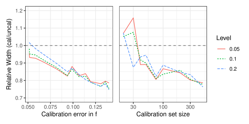
(b) Relative efficiency change from calibration.

Figure 1: Figure 1(a) shows the average interval widths for varying $\ell^{2}$-calibration errors in $f$. Figure 1(b) shows the relative change in average interval width using Venn-Abers calibrated versus uncalibrated predictions, with varying $\ell^{2}$-calibration error in $f$ (left), and calibration set size (right). Below the horizontal lines signifies efficiency gains for SC-CP.

5.3 Experiment 2: Coverage and Adaptivity

In this experiment, we illustrate how self-consistency of $\widehat{C}_{n}(X_{n+1})$ can, in some cases, translate to stronger conditional coverage guarantees. Here we take $n_{train}=n_{cal}=1000$ and $n_{test}=2500$, and no distribution shift ($\kappa_{train}=1$) in $\mathcal{D}_{train}$. We consider three setups: Setup A ($d=5,a=0,b=0.6$) and Setup B ($d=5,a=0,b=0.6$) which have a strong mean-variance relationship in the outcome process; and Setup C ($d=5,a=0.6,b=0$) which has no such relationship. We obtain the predictor $f$ from $\mathcal{D}_{train}$ using a generalized additive model (Hastie & Tibshirani, 1987), so that it is well calibrated and accurately estimates $\mu$. To assess the adaptivity of SC-CP to heteroscedasticity, we report the coverage and the average interval width within subgroups of $\mathcal{D}_{test}$ defined by quintiles of the conditional variances $\{\sigma^{2}(X_{i}):(X_{i},Y_{i})\in\mathcal{D}_{test}\}$.

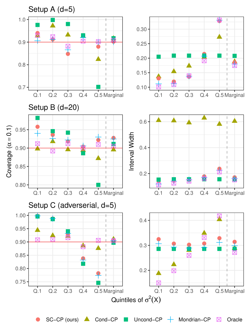
(a) Coverage and interval width for $\sigma^{2}(X)$ quintiles

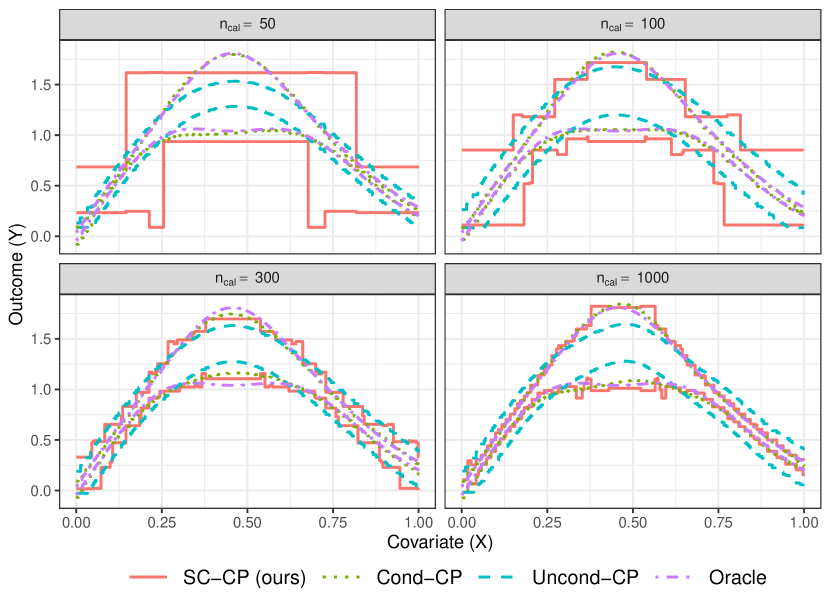
(b) Adaptivity of SC-CP with $n_{cal}$

Figure 2: Figure 2(a) displays the coverage and average interval width of SC-CP, marginally and within quintiles of the conditional outcome variance for setups A, B, and C. For a $d=1$ example, Figure 2(b) shows the adaptivity of SC-CP prediction bands ($\alpha=0.1$) across various calibration set sizes.

Results. The top two panels in Figure 2(a) displays the coverage and average interval width results for Setup A and Setup B. In both setups, SC-CP, cond-CP, and Mondrian-CP exhibit satisfactory coverage both marginally and within the quintile subgroups. In contrast, while uncond-CP attains the nominal level of marginal coverage, it exhibits noticeable overcoverage within the first three quintiles and significant undercoverage within the fifth quintile. The satisfactory performance of SC-CP with respect to heteroscedasticity in Setups A and B can be attributed to the strong mean-variance relationship in the outcome process. Regarding efficiency, the average interval widths of SC-CP are competitive with those of prediction-binned Mondrian-CP and the oracle intervals. The interval widths for cond-CP are wider than those for SC-CP and Mondrian-CP, especially for Setup B. This difference can be explained by cond-CP aiming for conditional validity in a 5D and 20D space, whereas SC-CP and Mondrian-CP target the 1D output space.

Limitation. If there is no mean-variance relationship in the outcomes, SC-CP is generally not expected to adapt to heteroscedasticity. The third (bottom) panel of Figure 2(a) displays SC-CP’s performance in Setup C, where there is no such relationship. In this scenario, it is evident that the conditional coverage of both uncond-CP and SC-CP are poor, while cond-CP maintains adequate coverage.

Adaptivity and calibration set size. SC-CP can be derived by applying CP within subgroups defined by a data-dependent binning of the output space $f(\mathcal{X})$, learned via Venn-Abers calibration, where the number of bins grows with $n_{cal}$. As $n_{\text{cal}}$ increases, the self-consistency result in Theorem 4.2 translates to conditional guarantees over finer partitions of $f(\mathcal{X})$. For $d=1$ and a strong mean-variance relationship ($a=0,b=0.6$), Figure 2(b) demonstrates how the adaptivity of SC-CP bands improves as $n_{\text{cal}}$ increases. In this case, for $n_{\text{cal}}$ sufficiently large, we find that the prediction bands of SC-CP closely match those of cond-CP and the oracle.

Impact statement. This paper presents work whose goal is to advance the field of Machine Learning. There are many potential societal consequences of our work, none which we feel must be specifically highlighted here.

Appendix A Code

Code implementing SC-CP and for reproducing our experiments can be found at this link: .

Appendix B Proofs

Proof of Theorem 4.1.

Recall from Algorithm 1 that $f_{n}^{(X_{n+1},Y_{n+1})}=\theta_{n}^{(X_{n+1},Y_{n+1})}\circ f$, where $\theta_{n}^{(X_{n+1},Y_{n+1})}\in\Theta_{iso}$ is an isotonic calibrator satisfying $f_{n}^{(X_{n+1},Y_{n+1})}=\theta_{n}^{(X_{n+1},Y_{n+1})}\circ f$. By definition, recall that the isotonic calibrator class $\Theta_{iso}$ satisfies the invariance property that, for all $g:\mathbb{R}\rightarrow\mathbb{R}$, the inclusion $\theta\in\Theta_{iso}$ implies $g\circ\theta\in\Theta_{iso}$. Hence, for all $g:\mathbb{R}\rightarrow\mathbb{R}$ and $\varepsilon>0$, it also holds that $(1+\varepsilon g)\circ\theta_{n}^{(X_{n+1},Y_{n+1})}$ lies in $\Theta_{iso}$. Now, we use that $(1+\varepsilon g)\circ\theta_{n}^{(X_{n+1},Y_{n+1})}\circ f=(1+\varepsilon g)\circ f_{n}^{(X_{n+1},Y_{n+1})}$ and that $f_{n}^{(X_{n+1},Y_{n+1})}$ is an empirical risk minimizer over the class $\{g\circ f:g\in\Theta_{iso}\}$. Using these two observations, the first order derivative equations characterizing the empirical risk minimizer $f_{n}^{(X_{n+1},Y_{n+1})}$ imply, for all $g:\mathbb{R}\rightarrow\mathbb{R}$, that

$$\frac{1}{n+1}\sum_{i=1}^{n+1}(g\circ f_{n}^{(X_{n+1},Y_{n+1})})(X_{i})\left\{Y_{i}-f_{n}^{(X_{n+1},Y_{n+1})}(X_{i})\right\} =\frac{d}{d\varepsilon}\left[\frac{1}{n+1}\sum_{i=1}^{n+1}\left\{Y_{i}-(1+\varepsilon g)\circ f_{n}^{(X_{n+1},Y_{n+1})}\right\}^{2}\right]\Bigg{|}_{\varepsilon=0}$$

$$=0.$$ (3)

Taking expectations of both sides of the above display, we conclude

$$\frac{1}{n+1}\sum_{i=1}^{n+1}\mathbb{E}\left[(g\circ f_{n}^{(X_{n+1},Y_{n+1})})(X_{i})\left\{Y_{i}-f_{n}^{(X_{n+1},Y_{n+1})}(X_{i})\right\}\right]=0.$$ (4)

We now use the fact that $\{(X_{i},Y_{i},f_{n}^{(X_{n+1},Y_{n+1})}(X_{i})):i\in[n+1]\}$ are exchangeable, since $\{(X_{i},Y_{i})\}_{i=1}^{n+1}$ are exchangeable by C1 and the function $f_{n}^{(X_{n+1},Y_{n+1})}$ is invariant under permutations of $\{(X_{i},Y_{i})\}_{i=1}^{n+1}$. Consequently, Equation (4) remains true if we replace each $(X_{i},Y_{i},f_{n}^{(X_{n+1},Y_{n+1})}(X_{i}))$ with $i\in[n]$ by $(X_{n+1},Y_{n+1},f_{n}^{(X_{n+1},Y_{n+1})}(X_{n+1}))$. That is,

$$\mathbb{E}\left[(g\circ f_{n}^{(X_{n+1},Y_{n+1})})(X_{n+1})\left\{Y_{n+1}-f_{n}^{(X_{n+1},Y_{n+1})}(X_{n+1})\right\}\right] =\frac{1}{n+1}\sum_{i=1}^{n+1}\mathbb{E}\left[(g\circ f_{n}^{(X_{n+1},Y_{n+1})})(X_{n+1})\left\{Y_{n+1}-f_{n}^{(X_{n+1},Y_{n+1})}(X_{n+1})\right\}\right]$$

$$=\frac{1}{n+1}\sum_{i=1}^{n+1}\mathbb{E}\left[(g\circ f_{n}^{(X_{n+1},Y_{n+1})})(X_{i})\left\{Y_{i}-f_{n}^{(X_{n+1},Y_{n+1})}(X_{i})\right\}\right]$$

$$=0.$$

By the law of iterated conditional expectations, the preceding display further implies

$$\mathbb{E}\left[(g\circ f_{n}^{(X_{n+1},Y_{n+1})})(X_{n+1})\left\{\mathbb{E}[Y_{n+1}\mid f_{n}^{(X_{n+1},Y_{n+1})}(X_{n+1})]-f_{n}^{(X_{n+1},Y_{n+1})}(X_{n+1})\right\}\right]=0.$$

Taking $g:\mathbb{R}\rightarrow\mathbb{R}$ to be defined by $(g\circ f_{n}^{(X_{n+1},Y_{n+1})})(X_{n+1}):=\mathbb{E}[Y_{n+1}\mid f_{n}^{(X_{n+1},Y_{n+1})}(X_{n+1})]-f_{n}^{(X_{n+1},Y_{n+1})}(X_{n+1})$, we find

$$\mathbb{E}\left[\left\{\mathbb{E}[Y_{n+1}\mid f_{n}^{(X_{n+1},Y_{n+1})}(X_{n+1})]-f_{n}^{(X_{n+1},Y_{n+1})}(X_{n+1})\right\}^{2}\right]=0.$$

The above equality implies $\mathbb{E}[Y_{n+1}\mid f_{n}^{(X_{n+1},Y_{n+1})}(X_{n+1})]=f_{n}^{(X_{n+1},Y_{n+1})}(X_{n+1})$ almost surely, as desired.

∎

Proof of Theorem 4.2.

This proof of this theorem follows from a modification of the arguments used to establish Theorem 2 of Gibbs et al. 2023. As in Gibbs et al. 2023, we begin by examining the first-order equations of the convex optimization problem defining $\rho_{n}^{(X_{n+1},Y_{n+1})}$ in Algorithm 2.

Recall, for a quantile level $\alpha\in(0,1)$, the “pinball” quantile loss function $\ell_{\alpha}$ is given by

$$\ell_{\alpha}(f(x),s):=\begin{cases}\alpha(s-f(x))&\text{if }s\geq f(x),\\ (1-\alpha)(f(x)-s)&\text{if }s<f(x).\end{cases}$$

As established in Gibbs et al. 2023, each subgradient of $\ell_{\alpha}(\cdot,x)$ at $f$ in the direction $g$, for some $\beta\in[\alpha-1,\alpha]$, given by:

$$\partial_{\varepsilon[\beta]}\left\{\ell_{\alpha}(f(x)+\varepsilon g(x),s)\right\}\big{|}_{\varepsilon=0}:=1(f(x)\neq s)g(x)\{\alpha-1(f<s)\}+1(f(x)=s)\beta g(x).$$

Studying first-order equations of convex problem: Given any transformation $\theta:\mathbb{R}\rightarrow\mathbb{R}$, each subgradient of the map

$$\varepsilon\mapsto\ell_{\alpha}\left(\rho_{n}^{(X_{n+1},Y_{n+1})}(X_{i})+\varepsilon\theta\circ f_{n}^{(X_{n+1},Y_{n+1})}(X_{i}),S_{i}^{(X_{n+1},Y_{n+1})}\right)$$

is, for some $\beta\in[\alpha-1,\alpha]^{n+1}$, of the following form:

$$\partial_{\varepsilon[\beta]}\left\{\ell_{\alpha}\left(\rho_{n}^{(X_{n+1},Y_{n+1})}(X_{i})+\varepsilon\theta\circ f_{n}^{(X_{n+1},Y_{n+1})}(X_{i}),S_{i}^{(X_{n+1},Y_{n+1})}\right)\right\}\big{|}_{\varepsilon=0}$$

$$\hskip 28.45274pt:=\begin{cases}\theta\circ f_{n}^{(X_{n+1},Y_{n+1})}(X_{i})\{\alpha-1(\rho_{n}^{(X_{n+1},Y_{n+1})}(X_{i})<S_{i}^{(X_{n+1},Y_{n+1})})\}&\text{if }S_{i}^{(X_{n+1},Y_{n+1})}\neq\rho_{n}^{(X_{n+1},Y_{n+1})}(X_{i}),\\ \beta_{i}(\theta\circ f_{n}^{(X_{n+1},Y_{n+1})})(X_{i})&\text{if }S_{i}^{(X_{n+1},Y_{n+1})}\neq\rho_{n}^{(X_{n+1},Y_{n+1})}(X_{i}).\\ \end{cases}$$

Now, since $\rho_{n}^{(X_{n+1},Y_{n+1})}$ is an empirical risk minimizer of the quantile loss over the class $\{\theta\circ f_{n}^{(X_{n+1},Y_{n+1})};\,\theta:\mathbb{R}\rightarrow\mathbb{R}\}$, there exists some vector $\beta^{*}=(\beta_{1}^{*},\dots,\beta_{n+1}^{*})\in[\alpha-1,\alpha]^{n+1}$ such that

$$0 =\frac{1}{n+1}\sum_{i=1}^{n+1}1\{S_{i}^{(X_{n+1},Y_{n+1})}\neq\rho_{n}^{(X_{n+1},Y_{n+1})}(X_{i})\}\left[\theta\circ f_{n}^{(X_{n+1},Y_{n+1})}(X_{i})\{\alpha-1(\rho_{n}^{(X_{n+1},Y_{n+1})}(X_{i})<S_{i}^{(X_{n+1},Y_{n+1})})\}\right]$$

$$\quad+\frac{1}{n+1}\sum_{i=1}^{n+1}1\{S_{i}^{(X_{n+1},Y_{n+1})}=\rho_{n}^{(X_{n+1},Y_{n+1})}(X_{i})\}\left[\beta_{i}^{*}(\theta\circ f_{n}^{(X_{n+1},Y_{n+1})})(X_{i})\right]$$

The above display can be rewritten as:

$$\frac{1}{n+1}\sum_{i=1}^{n+1}\left[\theta\circ f_{n}^{(X_{n+1},Y_{n+1})}(X_{i})\{\alpha-1(\rho_{n}^{(X_{n+1},Y_{n+1})}(X_{i})<S_{i}^{(X_{n+1},Y_{n+1})})\}\right]$$

$$\hskip 28.45274pt=\frac{1}{n+1}\sum_{i=1}^{n+1}1\{S_{i}^{(X_{n+1},Y_{n+1})}=\rho_{n}^{(X_{n+1},Y_{n+1})}(X_{i})\}\left[(1-\beta_{i}^{*})(\theta\circ f_{n}^{(X_{n+1},Y_{n+1})})(X_{i})\right].$$ (5)

Now, observe that the collection of random variables

$$\left\{(f_{n}^{(X_{n+1},Y_{n+1})}(X_{i}),S_{i}^{(X_{n+1},Y_{n+1})},\rho_{n}^{(X_{n+1},Y_{n+1})}(X_{i})):i\in[n+1]\right\}$$

are exchangeable, since $\{((X_{i},Y_{i}),f(X_{i})):i\in[n+1]\}$ are exchangeable by C1 and, for any $x\in\mathcal{X}$, the set $\{(f_{n}^{(X_{n+1},Y_{n+1})}(x),S_{i}^{(X_{n+1},Y_{n+1})}(x),\rho_{n}^{(X_{n+1},Y_{n+1})}(x)):i\in[n+1]\}$ is invariant under permutations of $\{(X_{i},Y_{i})\}_{i\in[n+1]}$. Thus, the expectation of the left-hand side of Equation (5) can be expressed as:

$$\mathbb{E}\left[\frac{1}{n+1}\sum_{i=1}^{n+1}\left[\theta\circ f_{n}^{(X_{n+1},Y_{n+1})}(X_{i})\{\alpha-1(\rho_{n}^{(X_{n+1},Y_{n+1})}(X_{i})<S_{i}^{(X_{n+1},Y_{n+1})})\}\right]\right]$$

$$\hskip 28.45274pt=\frac{1}{n+1}\sum_{i=1}^{n+1}\mathbb{E}\left[\theta\circ f_{n}^{(X_{n+1},Y_{n+1})}(X_{i})\{\alpha-1(\rho_{n}^{(X_{n+1},Y_{n+1})}(X_{i})<S_{i}^{(X_{n+1},Y_{n+1})})\}\right]$$

$$\hskip 28.45274pt=\mathbb{E}\left[\theta\circ f_{n}^{(X_{n+1},Y_{n+1})}(X_{n+1})\{\alpha-1(\rho_{n}^{(X_{n+1},Y_{n+1})}(X_{n+1})<S_{n+1}^{(X_{n+1},Y_{n+1})})\}\right],$$

where the final inequality follows from exchangeability. Combining this with Equation (5), we find

$$\mathbb{E}\left[\theta\circ f_{n}^{(X_{n+1},Y_{n+1})}(X_{n+1})\{\alpha-1(\rho_{n}^{(X_{n+1},Y_{n+1})}(X_{n+1})<S_{n+1}^{(X_{n+1},Y_{n+1})})\}\right]$$ (6)

$$\hskip 28.45274pt=\mathbb{E}\left[1\{S_{i}^{(X_{n+1},Y_{n+1})}=\rho_{n}^{(X_{n+1},Y_{n+1})}(X_{i})\}\left[(1-\beta_{i}^{*})(\theta\circ f_{n}^{(X_{n+1},Y_{n+1})})(X_{i})\right]\right|$$ (7)

Lower bound on coverage: We first obtain the lower coverage bound in the theorem statement. Note, for any nonnegative $f:\mathbb{R}\rightarrow\mathbb{R}$, that (7) implies:

$$\mathbb{E}\left[\theta\circ f_{n}^{(X_{n+1},Y_{n+1})}(X_{n+1})\{\alpha-1(\rho_{n}^{(X_{n+1},Y_{n+1})}(X_{n+1})<S_{n+1}^{(X_{n+1},Y_{n+1})})\}\right]\geq 0.$$

This inequality holds since $(1-\beta^{*}_{i})\geq 0$ and $(\theta\circ f_{n}^{(X_{n+1},Y_{n+1})})(X_{i})\geq 0$ almost surely, for each $i\in[n+1]$.

By the law of iterated expectations, we then have

$$\mathbb{E}\left[\theta\circ f_{n}^{(X_{n+1},Y_{n+1})}(X_{n+1})\left\{\alpha-\mathbb{P}\left(\rho_{n}^{(X_{n+1},Y_{n+1})}(X_{n+1})<S_{n+1}^{(X_{n+1},Y_{n+1})}\mid f_{n}^{(X_{n+1},Y_{n+1})}(X_{n+1})\right)\right\}\right]\geq 0.$$

Taking $\theta:\mathbb{R}\rightarrow\mathbb{R}$ as a nonnegative map that almost surely satisfies

$$\theta\circ f_{n}^{(X_{n+1},Y_{n+1})}(X_{n+1})=1\left\{\alpha\leq\mathbb{P}\left(\rho_{n}^{(X_{n+1},Y_{n+1})}(X_{n+1})<S_{n+1}^{(X_{n+1},Y_{n+1})}\mid f_{n}^{(X_{n+1},Y_{n+1})}(X_{n+1})\right)\right\},$$

we find

$$-\mathbb{E}\left[\left\{\alpha-\mathbb{P}\left(\rho_{n}^{(X_{n+1},Y_{n+1})}(X_{n+1})<S_{n+1}^{(X_{n+1},Y_{n+1})}\mid f_{n}^{(X_{n+1},Y_{n+1})}(X_{n+1})\right)\right\}_{-}\right]\geq 0,$$

where the map $t\mapsto\{t\}_{-}:=|t|1(t\leq 0)$ extracts the negative part of its input. Multiplying both sides of the previous inequality by $-1$, we obtain

$$0\leq\mathbb{E}\left[\left\{\alpha-\mathbb{P}\left(\rho_{n}^{(X_{n+1},Y_{n+1})}(X_{n+1})<S_{n+1}^{(X_{n+1},Y_{n+1})}\mid f_{n}^{(X_{n+1},Y_{n+1})}(X_{n+1})\right)\right\}_{-}\right]\leq 0.$$

We conclude that the negative part of $\left\{\alpha-\mathbb{P}\left(\rho_{n}^{(X_{n+1},Y_{n+1})}(X_{n+1})<S_{n+1}^{(X_{n+1},Y_{n+1})}\mid f_{n}^{(X_{n+1},Y_{n+1})}(X_{n+1})\right)\right\}$ is almost surely zero. Thus, it must be almost surely true that

$$\alpha\geq\mathbb{P}\left(\rho_{n}^{(X_{n+1},Y_{n+1})}(X_{n+1})<S_{n+1}^{(X_{n+1},Y_{n+1})}\mid f_{n}^{(X_{n+1},Y_{n+1})}(X_{n+1})\right).$$

Note that the event $Y_{n+1}\in\widehat{C}_{n}(X_{n+1})=\{y\in\mathcal{Y}:S_{n+1}^{(X_{n+1},y)}\leq\rho_{n}^{(X_{n+1},y)}(X_{n+1})\}$ occurs if, and only if, $\rho_{n}^{(X_{n+1},Y_{n+1})}(X_{n+1})\geq S_{n+1}^{(X_{n+1},Y_{n+1})}$. As a result, we obtain the desired lower coverage bound:

$$1-\alpha\leq\mathbb{P}\left(Y_{n+1}\in\widehat{C}_{n}(X_{n+1})\mid f_{n}^{(X_{n+1},Y_{n+1})}(X_{n+1})\right).$$

Deviation bound for the coverage: We now bound the deviation of the coverage of SC-CP from the lower bound. Note, for any $f:\mathbb{R}\rightarrow\mathbb{R}$, that (7) implies:

$$\mathbb{E}\left[\theta\circ f_{n}^{(X_{n+1},Y_{n+1})}(X_{n+1})\{\alpha-1(\rho_{n}^{(X_{n+1},Y_{n+1})}(X_{n+1})<S_{n+1}^{(X_{n+1},Y_{n+1})})\}\right]$$

$$\hskip 28.45274pt\leq\left|\mathbb{E}\left[1\{S_{i}^{(X_{n+1},Y_{n+1})}=\rho_{n}^{(X_{n+1},Y_{n+1})}(X_{i})\}\left[(1-\beta_{i}^{*})(\theta\circ f_{n}^{(X_{n+1},Y_{n+1})})(X_{i})\right]\right|\right|.$$ (8)

Using that $(1-\beta_{i}^{*})\in[0,1]$ and exchangeability, we can bound the right-hand side of the above as

$$\left|\mathbb{E}\left[\frac{1}{n+1}\sum_{i=1}^{n+1}1\{S_{i}^{(X_{n+1},Y_{n+1})}=\rho_{n}^{(X_{n+1},Y_{n+1})}(X_{i})\}\left[(1-\beta_{i}^{*})(\theta\circ f_{n}^{(X_{n+1},Y_{n+1})})(X_{i})\right]\right]\right|$$

$$\leq\frac{1}{n+1}\mathbb{E}\left[\left\{\max_{i\in[n+1]}\left|(\theta\circ f_{n}^{(X_{n+1},Y_{n+1})})(X_{i})\right|\right\}\sum_{i=1}^{n+1}1\{S_{i}^{(X_{n+1},Y_{n+1})}=\rho_{n}^{(X_{n+1},Y_{n+1})}(X_{i})\}\right].$$

Next, since there are no ties by C3, the event $1\{S_{i}^{(X_{n+1},Y_{n+1})}=\rho_{n}^{(X_{n+1},Y_{n+1})}(X_{i})\}$ for some index $i\in[n+1]$ can only occur once per piecewise constant segment of $\rho_{n}^{(X_{n+1},Y_{n+1})}$, since, otherwise, $S_{i}^{(X_{n+1},Y_{n+1})}=\rho_{n}^{(X_{n+1},Y_{n+1})}(X_{i})=\rho_{n}^{(X_{n+1},Y_{n+1})}(X_{j})=S_{j}^{(X_{n+1},Y_{n+1})}$ for some $i\neq j$. However, $\rho_{n}^{(X_{n+1},Y_{n+1})}$ is a transformation of $f_{n}^{(X_{n+1},Y_{n+1})}$ and, therefore, has the same number of constant segments as $f_{n}^{(X_{n+1},Y_{n+1})}$. In particular, by C2, $\rho_{n}^{(X_{n+1},Y_{n+1})}$ has no more than $n^{1/3}\operatorname*{polylog}(n)$ constant segments. It therefore holds that

$$\sum_{i=1}^{n+1}1\{S_{i}^{(X_{n+1},Y_{n+1})}=\rho_{n}^{(X_{n+1},Y_{n+1})}(X_{i})\}\leq n^{1/3}\operatorname*{polylog}(n).$$

Using that $\frac{n^{1/3}\operatorname*{polylog}(n)}{n+1}\leq\frac{\operatorname*{polylog}(n)}{n^{2/3}}$, this implies that

$$\frac{1}{n+1}\mathbb{E}\left[\max_{i\in[n+1]}|(\theta\circ f_{n}^{(X_{n+1},Y_{n+1})})(X_{i})|\sum_{i=1}^{n+1}1\{S_{i}^{(X_{n+1},Y_{n+1})}=\rho_{n}^{(X_{n+1},Y_{n+1})}(X_{i})\}\right]\leq\frac{\operatorname*{polylog}(n)}{n^{2/3}}\mathbb{E}\left[\max_{i\in[n+1]}|(\theta\circ f_{n}^{(X_{n+1},Y_{n+1})})(X_{i})|\right].$$

Combining this bound with (8), we find

$$\mathbb{E}\left[\theta\circ f_{n}^{(X_{n+1},Y_{n+1})}(X_{n+1})\{\alpha-1(\rho_{n}^{(X_{n+1},Y_{n+1})}(X_{n+1})<S_{n+1}^{(X_{n+1},Y_{n+1})})\}\right]\leq\frac{\operatorname*{polylog}(n)}{n^{2/3}}\mathbb{E}\left[\max_{i\in[n+1]}|(\theta\circ f_{n}^{(X_{n+1},Y_{n+1})})(X_{i})|\right].$$

By the law of iterated expectations, we then have

$$\mathbb{E}\left[\theta\circ f_{n}^{(X_{n+1},Y_{n+1})}(X_{n+1})\left\{\alpha-\mathbb{P}\left(\rho_{n}^{(X_{n+1},Y_{n+1})}(X_{n+1})<S_{n+1}^{(X_{n+1},Y_{n+1})}\mid f_{n}^{(X_{n+1},Y_{n+1})}(X_{n+1})\right)\right\}\right]$$

$$\hskip 28.45274pt\leq\frac{\operatorname*{polylog}(n)}{n^{2/3}}\mathbb{E}\left[\max_{i\in[n+1]}|(\theta\circ f_{n}^{(X_{n+1},Y_{n+1})})(X_{i})|\right].$$

Next, let $\mathcal{V}\subset\mathbb{R}$ denote the support of the random variable $f_{n}^{(X_{n+1},Y_{n+1})}(X_{n+1})$. Then, taking $\theta$ to be $t\mapsto 1(t\in\mathcal{V})\text{sign}\left\{\alpha-\mathbb{P}\left(\rho_{n}^{(X_{n+1},Y_{n+1})}(X_{n+1})<S_{n+1}^{(X_{n+1},Y_{n+1})}\mid f_{n}^{(X_{n+1},Y_{n+1})}(X_{n+1})=t\right)\right\}$, which falls almost surely in $\{-1,1\}$, we obtain the mean absolute error bound:

$$\mathbb{E}\left|\alpha-\mathbb{P}\left(\rho_{n}^{(X_{n+1},Y_{n+1})}(X_{n+1})<S_{n+1}^{(X_{n+1},Y_{n+1})}\mid f_{n}^{(X_{n+1},Y_{n+1})}(X_{n+1})\right)\right|\leq\frac{\operatorname*{polylog}(n)}{n^{2/3}}.$$

The result then follows noting that the event $Y_{n+1}\not\in\widehat{C}_{n}(X_{n+1})=\{y\in\mathcal{Y}:S_{n+1}^{(X_{n+1},y)}\leq\rho_{n}^{(X_{n+1},y)}(X_{n+1})\}$ occurs if, and only if, $\rho_{n}^{(X_{n+1},Y_{n+1})}(X_{n+1})<S_{n+1}^{(X_{n+1},Y_{n+1})}$.

∎

Proof of Theorem 4.3.

Let $P_{n+1}$ denote the empirical distribution of $\{(X_{i},Y_{i})\}_{i=1}^{n+1}$ and let $P_{n}$ denote the empirical distribution of $\{(X_{i},Y_{i})\}_{i=1}^{n}$. For any function $g:\mathcal{X}\times\mathcal{Y}\rightarrow\mathbb{R}$: we use the following empirical process notation: $Pg:=\int g(x,y)dP(x,y)$, $P_{n+1}g:=\int g(x,y)dP_{n+1}(x,y)$, and $P_{n}g:=\int g(x,y)dP_{n}(x,y)$.

Define the risk functions $R_{n}^{(x,y)}(\theta):=\frac{1}{n+1}\sum_{i=1}^{n}\{S_{\theta}(X_{i},Y_{i})\}^{2}+\frac{1}{n+1}\{S_{\theta}(x,y)\}^{2}$, $R_{n+1}(\theta):=\frac{1}{n+1}\sum_{i=1}^{n+1}\{S_{\theta}(X_{i},Y_{i})\}^{2}$, and $R_{0}(\theta):=\int\{S_{\theta}(x,y)\}^{2}dP(x,y)$. Moreover, define the risk minimizers as $\theta_{n}^{(x,y)}:=\operatorname*{argmin}_{\theta\in\Theta_{iso}}R_{n}^{(x,y)}(f)$ and $\theta_{0}:=\operatorname*{argmin}_{\theta\in\Theta_{iso}}R_{0}(\theta)$. Observe that $R_{n}^{(x,y)}(\theta_{n}^{(x,y)})-R_{n}^{(x,y)}(\theta_{0})\leq 0$ since $f_{n}$ minimizes $R_{n}$ over $\Theta_{iso}$. Using this inequality, it follows that

$$R_{0}(\theta_{n}^{(x,y)})-R_{0}(\theta_{0}) =R_{0}(\theta_{n}^{(x,y)})-R_{n}^{(x,y)}(\theta_{n}^{(x,y)})$$

$$\quad+R_{n}^{(x,y)}(\theta_{n}^{(x,y)})-R_{n}^{(x,y)}(\theta_{0})+R_{n}^{(x,y)}(\theta_{0})-R_{0}(\theta_{0})$$

$$\leq R_{0}(\theta_{n}^{(x,y)})-R_{n}^{(x,y)}(\theta_{n}^{(x,y)})-\left\{R_{n}^{(x,y)}(\theta_{0})-R_{0}(\theta_{0})\right\}$$

$$\leq R_{0}(\theta_{n}^{(x,y)})-R_{n+1}(\theta_{n}^{(x,y)})-\left\{R_{n+1}(\theta_{0})-R_{0}(\theta_{0})\right\}$$

$$\quad+R_{n}^{(x,y)}(\theta_{n}^{(x,y)})-R_{n+1}(\theta_{n}^{(x,y)})-\left\{R_{n}^{(x,y)}(\theta_{0})-R_{n+1}(\theta_{0})\right\}.$$

The first term on the right-hand side of the above display can written as

$$R_{0}(\theta_{n}^{(x,y)})-R_{n+1}(\theta_{n}^{(x,y)})-\left\{R_{n+1}(\theta_{0})-R_{0}(\theta_{0})\right\}=(P_{n+1}-P)\left[\{S_{\theta_{n}^{(x,y)}}\}^{2}-\{S_{\theta_{0}}\}^{2}\right].$$

We now bound the second term, $R_{n}^{(x,y)}(\theta_{n}^{(x,y)})-R_{n+1}(\theta_{n}^{(x,y)})-\left\{R_{n}^{(x,y)}(\theta_{0})-R_{n+1}(\theta_{0})\right\}$. For any $\theta\in\Theta_{iso}$, observe that

$$R_{n}^{(x,y)}(\theta)-R_{n+1}(\theta)=\frac{1}{n+1}\left[\{y-\theta\circ f(x)\}^{2}-\{Y_{n+1}-\theta\circ f(X_{n+1})\}^{2}\right].$$

We know that $\theta_{n}^{(x,y)}$ and $\theta_{0}$, being defined via isotonic regression, are uniformly bounded by $B:=\sup_{y\in\mathcal{Y}}|y|$, which is finite by C6. Therefore,

$$\left|R_{n}^{(x,y)}(\theta_{n}^{(x,y)})-R_{n+1}(\theta_{n}^{(x,y)})-\left\{R_{n}^{(x,y)}(\theta_{0})-R_{n+1}(\theta_{0})\right\}\right|\leq\frac{8B^{2}}{n+1}=O(n^{-1}).$$

Combining the previous displays, we obtain the excess risk bound

$$R_{0}(\theta_{n}^{(x,y)})-R_{0}(\theta_{0})\leq(P_{n+1}-P)\left[\{S_{\theta_{n}^{(x,y)}}\}^{2}-\{S_{\theta_{0}}\}^{2}\right]+O(n^{-1}).$$ (9)

Next, we claim that $R_{0}(\theta_{n}^{(x,y)})-R_{0}(\theta_{0})\geq\|(\theta_{n}^{(x,y)}\circ f)-(\theta_{0}\circ f)\|_{P}^{2}$. To show this, expanding the squares, note, pointwise for each $x\in\mathcal{X}$ and $y\in\mathcal{Y}$, that

$$\{S_{\theta_{n}^{(x,y)}}(x,y)\}^{2}-\{S_{\theta_{0}}(x,y)\}^{2} =\{\theta_{n}^{(x,y)}\circ f(x)\}^{2}-\{\theta_{0}\circ f(x)\}^{2}-2y\left\{(\theta_{n}^{(x,y)}\circ f)(x)-(\theta_{0}\circ f)(x)\right\}$$

$$=\left\{(\theta_{n}^{(x,y)}\circ f)(x)+(\theta_{0}\circ f)(x)-2y\right\}\left\{(\theta_{n}^{(x,y)}\circ f)(x)-(\theta_{0}\circ f)(x)\right\}.$$

Consequently,

$$R_{0}(\theta_{n}^{(x,y)})-R_{0}(\theta_{0})=\int\left\{(\theta_{n}^{(x,y)}\circ f)(x)+(\theta_{0}\circ f)(x)-2y\right\}\left\{(\theta_{n}^{(x,y)}\circ f)(x)-(\theta_{0}\circ f)(x)\right\}dP(x).$$ (10)

By C4, $\Theta_{iso}$ consists of all isotonic regression trees and is, therefore, a convex space ince $\Theta_{iso}$ is maximal by C4. Thus, the first order derivative equations defining the population minimizer $\theta_{0}$ imply that

$$\int\left\{\theta_{n}^{(x,y)}\circ f(x)-\theta_{0}\circ f(x)\right\}\left\{y-\theta_{0}\circ f(x)\right\}dP(x,y)\leq 0.$$ (11)

Combining (10) and (11), we find

$$R_{0}(\theta_{n}^{(x,y)})-R_{0}(\theta_{0}) =\int\left\{(\theta_{n}^{(x,y)}\circ f)(x)-(\theta_{0}\circ f)(x)\right\}^{2}dP(x)$$

$$\quad+2\int\left\{(\theta_{0}\circ f)(x)-y\right\}\left\{(\theta_{n}^{(x,y)}\circ f)(x)-(\theta_{0}\circ f)(x)\right\}dP(x)$$

$$\geq\int\left\{(\theta_{n}^{(x,y)}\circ f)(x)-(\theta_{0}\circ f)(x)\right\}^{2}dP(x),$$

as desired. Combining this lower bound with (9), we obtain the inequality

$$\int\left\{(\theta_{n}^{(x,y)}\circ f)(x)-(\theta_{0}\circ f)(x)\right\}^{2}dP(x)\leq R_{0}(\theta_{n}^{(x,y)})-R_{0}(\theta_{0})\leq(P_{n}-P)\left[\{S_{\theta_{n}^{(x,y)}}\}^{2}-\{S_{\theta_{0}}\}^{2}\right]+O(1/n)$$ (12)

Define $\delta_{n}:=\sqrt{\int\left\{(\theta_{n}^{(x,y)}\circ f)(x)-(\theta_{0}\circ f)(x)\right\}^{2}dP(x)}$, the bound $B:=\sup_{y\in\mathcal{Y}}|y|$, and the function class,

$$\Theta_{1,n}:=\left\{(x,y)\mapsto\{(\theta_{1}+\theta_{2})\circ f-2y\}\{(\theta_{1}-\theta_{2})\circ f\}\right\}.$$

Using this notation, (12) implies

$$\delta_{n}^{2} \leq\sup_{\theta_{1},\theta_{2}\in\Theta_{iso}:\left\lVert\theta_{1}-\theta_{2}\right\rVert\leq\delta_{n}}\int\{(\theta_{1}+\theta_{2})\circ f(x)-2y\}\{(\theta_{1}-\theta_{2})\circ f(x)\}d(P_{n}-P)(x,y)+O(1/n)$$

$$\leq\sup_{h\in\Theta_{1,n}:\left\lVert h\right\rVert\leq 4B\delta_{n}}(P_{n}-P)h+O(1/n)$$

Using the above inequality and C5, we will use an argument nearly identical to the proof of Theorem 3 in van der Laan et al. 2023 to establish that $\delta_{n}=O_{p}(n^{-1/3})$. By (12), this rate will then imply that $R_{0}(\theta_{n}^{(x,y)})-R_{0}(\theta_{0})=O_{p}(n^{-2/3})$, which establishes the first statement of the theorem.

We now sketch the argument that $\delta_{n}=O_{p}(n^{-1/3})$. For a function class $\mathcal{F}$, let $N(\epsilon,\mathcal{F},L_{2}(P))$ denote the $\epsilon-$covering number (van der Vaart & Wellner, 1996) of $\mathcal{F}$ and define the uniform entropy integral of $\mathcal{F}$ by

$$\mathcal{J}(\delta,\mathcal{F}):=\int_{0}^{\delta}\sup_{Q}\sqrt{\log N(\epsilon,\mathcal{F},L_{2}(Q))}\,d\epsilon\ ,$$

where the supremum is taken over all discrete probability distributions $Q$. We note that

$$\mathcal{J}(\delta,\Theta_{1,n}) =\int_{0}^{\delta}\sup_{Q}\sqrt{N(\varepsilon,\Theta_{1,n},\left\lVert\,\cdot\,\right\rVert_{Q})}\,d\varepsilon=\int_{0}^{\delta}\sup_{Q}\sqrt{N(\varepsilon,\Theta_{iso},\left\lVert\,\cdot\,\right\rVert_{Q\circ f^{-1}})}\,d\varepsilon=\mathcal{J}(\delta,\Theta_{iso})\ ,$$

where $Q\circ f^{-1}$ is the push-forward probability measure for the random variable $f(W)$. Additionally, the covering number bound for bounded monotone functions given in Theorem 2.7.5 of vanderVaartWellner implies that

$$\mathcal{J}(\delta,\Theta_{1,n})=\mathcal{J}(\delta,\Theta_{iso})\lesssim\sqrt{\delta}.$$

Recall that $f$ is obtained from an external dataset, say $\mathcal{E}_{n}$, independent of the calibration data. Noting that $f$ is deterministic conditional on a training dataset $\mathcal{E}_{n}$. Applying Theorem 2.1 of Van Der Vaart & Wellner 2011 conditional on $\mathcal{E}_{n}$, we obtain, for any $\delta>0$, that

$$E\left[\sup_{h\in\Theta_{1,n}:\left\lVert h\right\rVert\leq 4B\delta}(P_{n}-P)h\,|\,\mathcal{E}_{n}\right] \lesssim\ n^{-1/2}\mathcal{J}(\delta,\Theta_{1,n})\left(1+\frac{\mathcal{J}(\delta,\Theta_{1,n})}{\sqrt{n}\delta^{2}}\right).$$

$$\lesssim\ n^{-1/2}\mathcal{J}(\delta,\Theta_{iso})\left(1+\frac{\mathcal{J}(\delta,\Theta_{iso})}{\sqrt{n}\delta^{2}}\right).$$

Noting that the right-hand side of the above bound is deterministic, we conclude that

$$E\left[\sup_{h\in\Theta_{1,n}:\left\lVert h\right\rVert\leq 4B\delta}(P_{n}-P)h\right]\lesssim n^{-1/2}\mathcal{J}(\delta,\Theta_{iso})\left(1+\frac{\mathcal{J}(\delta,\Theta_{iso})}{\sqrt{n}\delta^{2}}\right).$$

We use the so-called “peeling” argument (van der Vaart & Wellner, 1996) to obtain our bound for $\delta_{n}$. Note

$$P\left(\delta_{n}^{2}\geq n^{-2/3}2^{M}\right) =\sum_{m=M}^{\infty}P\left(2^{m+1}\geq n^{2/3}\delta_{n}^{2}\geq 2^{m}\right)$$

$$=\sum_{m=M}^{\infty}P\left(2^{m+1}\geq n^{2/3}\delta_{n}^{2}\geq 2^{m}\,,\delta_{n}^{2}\leq\sup_{h\in\Theta_{1,n}:\left\lVert h\right\rVert\leq 4B\delta_{n}}(P_{n}-P)h+O(1/n)\right)$$

$$=\sum_{m=M}^{\infty}P\left(2^{m+1}\geq n^{2/3}\delta_{n}^{2}\geq 2^{m}\,,2^{2m}n^{-2/3}\leq\sup_{h\in\Theta_{1,n}:\left\lVert h\right\rVert\leq 4B2^{m+1}n^{-1/3}}(P_{n}-P)h+O(1/n)\right)$$

$$\leq\sum_{m=M}^{\infty}P\left(2^{2m}n^{-2/3}\leq\sup_{h\in\Theta_{1,n}:\left\lVert h\right\rVert\leq 4B2^{m+1}n^{-1/3}}(P_{n}-P)h+O(1/n)\right)$$

$$\leq\sum_{m=M}^{\infty}\frac{E\left[\sup_{h\in\Theta_{1,n}:\left\lVert h\right\rVert\leq 4B2^{m+1}n^{-1/3}}(P_{n}-P)h\right]+O(1/n)}{2^{2m}n^{-2/3}}$$

$$\leq\sum_{m=M}^{\infty}\frac{\mathcal{J}(2^{m+1}n^{-1/3},\Theta_{iso})\left(1+\frac{\mathcal{J}(2^{2m+2}n^{-2/3},\Theta_{iso})}{\sqrt{n}2^{m+1}n^{-1/3}}\right)}{\sqrt{n}2^{2m}n^{-2/3}}+\sum_{m=M}^{\infty}\frac{O(1/n)}{2^{2m}n^{-2/3}}$$

$$\leq\sum_{m=M}^{\infty}\frac{2^{(m+1)/2}n^{-1/6}}{2^{2m}n^{-1/6}}+\sum_{m=M}^{\infty}\frac{o(1)}{2^{2m}}$$

$$\lesssim\sum_{m=M}^{\infty}\frac{2^{(m+1)/2}}{2^{2m}}.$$

Since $\sum_{m=1}^{\infty}\frac{2^{(m+1)/2}}{2^{2m}}<\infty$, we have that $\sum_{m=M}^{\infty}\frac{2^{(m+1)/2}}{2^{2m}}\rightarrow 0$ as $M\rightarrow\infty$. Therefore, for all $\varepsilon>0$, we can choose $M>0$ large enough so that

$$P\left(\delta_{n}^{2}\geq n^{-2/3}2^{M}\right)\leq\varepsilon.$$

We conclude that $\delta_{n}=O_{p}(n^{-1/3})$ as desired.

∎

References

• Awaysheh et al. (2019) Awaysheh, A., Wilcke, J., Elvinger, F., Rees, L., Fan, W., and Zimmerman, K. L. Review of medical decision support and machine-learning methods. Veterinary pathology, 56(4):512–525, 2019.
• Balasubramanian et al. (2014) Balasubramanian, V., Ho, S.-S., and Vovk, V. Conformal prediction for reliable machine learning: theory, adaptations and applications. Newnes, 2014.
• Barber et al. (2021) Barber, R., Candes, E. J., Ramdas, A., and Tibshirani, R. J. The limits of distribution-free conditional predictive inference. Information and Inference: A Journal of the IMA, 10(2):455–482, 2021.
• Barlow & Brunk (1972) Barlow, R. E. and Brunk, H. D. The isotonic regression problem and its dual. Journal of the American Statistical Association, 67(337):140–147, 1972.
• Bhardwaj et al. (2017) Bhardwaj, R., Nambiar, A. R., and Dutta, D. A study of machine learning in healthcare. In 2017 IEEE 41st annual computer software and applications conference (COMPSAC), volume 2, pp.  236–241. IEEE, 2017.
• Boström & Johansson (2020) Boström, H. and Johansson, U. Mondrian conformal regressors. In Conformal and Probabilistic Prediction and Applications, pp.  114–133. PMLR, 2020.
• Boström et al. (2021) Boström, H., Johansson, U., and Löfström, T. Mondrian conformal predictive distributions. In Conformal and Probabilistic Prediction and Applications, pp.  24–38. PMLR, 2021.
• Caponnetto & Rakhlin (2006) Caponnetto, A. and Rakhlin, A. Stability properties of empirical risk minimization over donsker classes. Journal of Machine Learning Research, 7(12), 2006.
• Char et al. (2018) Char, D. S., Shah, N. H., and Magnus, D. Implementing machine learning in health care—addressing ethical challenges. The New England journal of medicine, 378(11):981, 2018.
• Chen & Guestrin (2016) Chen, T. and Guestrin, C. XGBoost: A scalable tree boosting system. In Proceedings of the 22nd ACM SIGKDD International Conference on Knowledge Discovery and Data Mining, KDD ’16, pp.  785–794, New York, NY, USA, 2016. ACM. ISBN 978-1-4503-4232-2. doi: 10.1145/2939672.2939785. URL http://doi.acm.org/10.1145/2939672.2939785.
• Dai et al. (2020) Dai, R., Song, H., Barber, R. F., and Raskutti, G. The bias of isotonic regression. Electronic journal of statistics, 14(1):801, 2020.
• Deng et al. (2021) Deng, H., Han, Q., and Zhang, C.-H. Confidence intervals for multiple isotonic regression and other monotone models. The Annals of Statistics, 49(4):2021–2052, 2021.
• Efron (1967) Efron, B. The two sample problem with censored data. In Proceedings of the fifth Berkeley symposium on mathematical statistics and probability, volume 4, pp.  831–853, 1967.
• Flury & Tarpey (1996) Flury, B. and Tarpey, T. Self-consistency: A fundamental concept in statistics. Statistical Science, 11(3):229–243, 1996.
• Gibbs et al. (2023) Gibbs, I., Cherian, J. J., and Candès, E. J. Conformal prediction with conditional guarantees. arXiv preprint arXiv:2305.12616, 2023.
• Gupta & Ramdas (2021) Gupta, C. and Ramdas, A. Distribution-free calibration guarantees for histogram binning without sample splitting. In International Conference on Machine Learning, pp. 3942–3952. PMLR, 2021.
• Gupta et al. (2020) Gupta, C., Podkopaev, A., and Ramdas, A. Distribution-free binary classification: prediction sets, confidence intervals and calibration. Advances in Neural Information Processing Systems, 33:3711–3723, 2020.
• Hastie & Tibshirani (1987) Hastie, T. and Tibshirani, R. Generalized additive models: some applications. Journal of the American Statistical Association, 82(398):371–386, 1987.
• Johansson et al. (2014) Johansson, U., Sönströd, C., Linusson, H., and Boström, H. Regression trees for streaming data with local performance guarantees. In 2014 IEEE International Conference on Big Data (Big Data), pp.  461–470. IEEE, 2014.
• Johansson et al. (2018) Johansson, U., Linusson, H., Löfström, T., and Boström, H. Interpretable regression trees using conformal prediction. Expert systems with applications, 97:394–404, 2018.
• Kang et al. (2015) Kang, J., Schwartz, R., Flickinger, J., and Beriwal, S. Machine learning approaches for predicting radiation therapy outcomes: a clinician’s perspective. International Journal of Radiation Oncology* Biology* Physics, 93(5):1127–1135, 2015.
• Lee et al. (2015) Lee, J., Maslove, D. M., and Dubin, J. A. Personalized mortality prediction driven by electronic medical data and a patient similarity metric. PloS one, 10(5):e0127428, 2015.
• Lei et al. (2018) Lei, J., G’Sell, M., Rinaldo, A., Tibshirani, R. J., and Wasserman, L. Distribution-free predictive inference for regression. Journal of the American Statistical Association, 113(523):1094–1111, 2018.
• Li et al. (2018) Li, Y., Qi, L., and Sun, Y. Semiparametric varying-coefficient regression analysis of recurrent events with applications to treatment switching. Statistics in Medicine, 37:3959–3974, 2018. doi: 10.1002/sim.7856. PubMed PMID: 29992591. NIHMSID: NIHMS1033642.
• Lloyd-Jones et al. (2019) Lloyd-Jones, D. M., Braun, L. T., Ndumele, C. E., Smith Jr, S. C., Sperling, L. S., Virani, S. S., and Blumenthal, R. S. Use of risk assessment tools to guide decision-making in the primary prevention of atherosclerotic cardiovascular disease: a special report from the american heart association and american college of cardiology. Circulation, 139(25):e1162–e1177, 2019.
• Mandinach et al. (2006) Mandinach, E. B., Honey, M., and Light, D. A theoretical framework for data-driven decision making. In annual meeting of the American Educational Research Association, San Francisco, CA, 2006.
• Marr (2019) Marr, B. Artificial intelligence in practice: how 50 successful companies used AI and machine learning to solve problems. John Wiley & Sons, 2019.
• Niculescu-Mizil & Caruana (2005) Niculescu-Mizil, A. and Caruana, R. Obtaining calibrated probabilities from boosting. In UAI, volume 5, pp.  413–20, 2005.
• Quest et al. (2018) Quest, L., Charrie, A., du Croo de Jongh, L., and Roy, S. The risks and benefits of using ai to detect crime. Harv. Bus. Rev. Digit. Artic, 8:2–5, 2018.
• Shafer & Vovk (2008) Shafer, G. and Vovk, V. A tutorial on conformal prediction. Journal of Machine Learning Research, 9(3), 2008.
• Sircar et al. (2021) Sircar, A., Yadav, K., Rayavarapu, K., Bist, N., and Oza, H. Application of machine learning and artificial intelligence in oil and gas industry. Petroleum Research, 6(4):379–391, 2021.
• van Calster et al. (2019) van Calster, B., McLernon, D. J., van Smeden, M., Wynants, L., and Steyerberg, E. W. Calibration: the achilles heel of predictive analytics. BMC medicine, 17(1):1–7, 2019.
• van der Laan et al. (2023) van der Laan, L., Ulloa-Pérez, E., Carone, M., and Luedtke, A. Causal isotonic calibration for heterogeneous treatment effects. In Proceedings of the 40th International Conference on Machine Learning (ICML), volume 202, Honolulu, Hawaii, USA, 2023. PMLR.
• van der Laan et al. (2023) van der Laan, L., Ulloa-Pérez, E., Carone, M., and Luedtke, A. Causal isotonic calibration for heterogeneous treatment effects. arXiv preprint arXiv:2302.14011, 2023.
• van der Vaart & Wellner (1996) van der Vaart, A. and Wellner, J. Weak Convergence and Empirical Processes. Springer, New York, 1996.
• Van Der Vaart & Wellner (2011) Van Der Vaart, A. and Wellner, J. A. A local maximal inequality under uniform entropy. Electronic Journal of Statistics, 5(2011):192, 2011.
• Veale et al. (2018) Veale, M., Van Kleek, M., and Binns, R. Fairness and accountability design needs for algorithmic support in high-stakes public sector decision-making. In Proceedings of the 2018 chi conference on human factors in computing systems, pp.  1–14, 2018.
• Vovk (2012) Vovk, V. Conditional validity of inductive conformal predictors. In Asian conference on machine learning, pp.  475–490. PMLR, 2012.
• Vovk & Petej (2012) Vovk, V. and Petej, I. Venn-abers predictors. arXiv preprint arXiv:1211.0025, 2012.
• Vovk et al. (2005) Vovk, V., Gammerman, A., and Shafer, G. Algorithmic learning in a random world, volume 29. Springer, 2005.
• Wright & Ziegler (2017) Wright, M. N. and Ziegler, A. ranger: A fast implementation of random forests for high dimensional data in C++ and R. Journal of Statistical Software, 77(1):1–17, 2017. doi: 10.18637/jss.v077.i01.
• Xu & Yadlowsky (2022) Xu, Y. and Yadlowsky, S. Calibration error for heterogeneous treatment effects. In International Conference on Artificial Intelligence and Statistics, pp.  9280–9303. PMLR, 2022.
• Zadrozny & Elkan (2002) Zadrozny, B. and Elkan, C. Transforming classifier scores into accurate multiclass probability estimates. In Proceedings of the eighth ACM SIGKDD international conference on Knowledge discovery and data mining, pp.  694–699, 2002.