Walsh’s Conformal Map onto Lemniscatic Domains for Several Intervals

Abstract

We consider Walsh’s conformal map from the complement of a compact set $E=\cup_{j=1}^{\ell}E_{j}$ with $\ell$ components onto a lemniscatic domain $\widehat{\mathbb{C}}\setminus L$, where $L$ has the form $L=\{w\in\mathbb{C}:\prod_{j=1}^{\ell}\lvert w-a_{j}\rvert^{m_{j}}\leq\operatorname{cap}(E)\}$. We prove that the exponents $m_{j}$ appearing in $L$ satisfy $m_{j}=\mu_{E}(E_{j})$, where $\mu_{E}$ is the equilibrium measure of $E$. When $E$ is the union of $\ell$ real intervals, we derive a fast algorithm for computing the centers $a_{1},\ldots,a_{\ell}$. For $\ell=2$, the formulas for $m_{1},m_{2}$ and $a_{1},a_{2}$ are explicit. Moreover, we obtain the conformal map numerically. Our approach relies on the real and complex Green’s functions of $\widehat{\mathbb{C}}\setminus E$ and $\widehat{\mathbb{C}}\setminus L$.

Keywords:

Conformal map, Lemniscatic domain, Multiply connected domain, Several intervals, Green’s function, Logarithmic capacity, Equilibrium measure.

AMS Subject Classification (2020):

30C35; 30C20; 30C85;

1 Introduction

When dealing with approximation problems on the interval $[-1,1]$, it is often convenient to formulate the problem on the unit circle by using the well-known Joukowsky map $z\mapsto{z}+\sqrt{z^{2}-1}$, which maps the complement of the interval $[-1,1]$ onto the complement of the unit disk, or its inverse $z\mapsto\frac{1}{2}(z+z^{-1})$. The mapping $z\mapsto{z}+\sqrt{z^{2}-1}$ is an example of the famous Riemann mapping theorem (setting $E:=[-1,1]$) which states that for each simply connected compact set $E$ there exists a unique (if suitably normalized at $z=\infty$) conformal map from the complement of $E$ to the complement of the unit disk. J. L. Walsh [23] found a rather canonical generalization for the case when $E$ is the union of $\ell$ simply connected compact sets. The corresponding conformal map $\Phi$ maps the complement of $E$ onto a so-called lemniscatic domain, which is a generalization of a classical lemniscate. More precisely, Walsh’s theorem reads as follows.

Theorem 1.1 ([23, Sect. III]).

Let $E_{1},\ldots,E_{\ell}\subseteq\mathbb{C}$ be disjoint simply connected, infinite compact sets and let

$$E=\bigcup_{j=1}^{\ell}E_{j},$$ (1.1)

that is, $E^{\operatorname{c}}\coloneq\widehat{\mathbb{C}}\setminus E$ is an $\ell$-connected domain. Then there exists a unique compact set $L$ of the form

$$L\coloneq\biggl{\{}w\in\mathbb{C}:\prod_{j=1}^{\ell}\lvert w-a_{j}\rvert^{m_{j}}\leq\operatorname{cap}(E)\biggr{\}},$$ (1.2)

where $a_{1},\ldots,a_{\ell}\in\mathbb{C}$ are pairwise distinct and $m_{1},\ldots,m_{\ell}>0$ are real with $\sum_{j=1}^{\ell}m_{j}=1$, and a unique conformal map

$$\Phi:E^{\operatorname{c}}\to L^{\operatorname{c}}\quad\text{with}\quad\Phi(z)=z+\mathcal{O}(1/z)\quad\text{at }\infty.$$ (1.3)

If $E$ is bounded by Jordan curves, then $\Phi$ extends to a homeomorphism from $\overline{E^{\operatorname{c}}}$ to $\overline{L^{\operatorname{c}}}$.

Let us note that the centers $a_{1},\ldots,a_{\ell}$ of $L$ and the exponents $m_{1},\ldots,m_{\ell}$ of $L$ in Theorem 1.1 are uniquely determined. The unbounded domain $L^{\operatorname{c}}$ is called a lemniscatic domain, see [7, p. 106].

Theorem 1.1 was first obtained by Walsh in his seminal 1956 paper [23]. Further existence proofs were published by Grunsky [5, 6, 7], Jenkins [8], and Landau [9]. None of these papers contain any explicit example, which might be the reason why Walsh’s map has not been widely used so far. However, in [26, pp. 374–377], Gaier recognizes this conformal map as one of Walsh’s major contributions. The first explicit examples of Walsh’s map were derived in [19]. In [12], Nasser, Liesen and the second author obtained a numerical method for computing Walsh’s map for sets $E$ bounded by smooth Jordan curves. This numerical algorithm also yields a method for the numerical computation of the logarithmic capacity of compact sets [10].

Walsh’s conformal map is intimately connected with several quantities from potential and approximation theory, including the logarithmic capacity $\operatorname{cap}(E)$, the equilibrium measure of $E$ (see Theorem 2.1 below), and the Green’s function of $L^{\operatorname{c}}$ and of $E^{\operatorname{c}}$, given respectively by the simple expressions

$$g_{L}(w)=\sum_{j=1}^{\ell}m_{j}\log\lvert w-a_{j}\rvert-\log(\operatorname{cap}(E))\quad\text{and}\quad g_{E}(z)=g_{L}(\Phi(z)).$$

Note that $g_{L}$ is harmonic in $\mathbb{C}\setminus\{a_{1},\ldots,a_{\ell}\}$, and has the simplest possible form.

An interesting application of Walsh’s conformal map in approximation theory is the construction of the Faber-Walsh polynomials of compact sets $E$ with several components as in Theorem 1.1; see Walsh’s original article [24], Suetin’s book [22], and the article [20]. Any function $f$ that is analytic on $E$ can be expanded in a series in the Faber-Walsh polynomials on $E$. The Faber-Walsh polynomials generalize the well-known Faber polynomials (defined on simply connected compact sets) and the Chebyshev polynomials of the first kind (on an interval). Liesen and the second author considered properties of the Faber-Walsh polynomials and gave the first explicit examples in [20], in particular in the case that $E$ is the union of two real intervals or two disks. For two symmetric intervals, the construction is explicit. In the present paper, we derive a way to numerically compute the conformal map for any number of real intervals, which will open up the way for polynomial approximation with Faber-Walsh polynomials on sets $E$ consisting of several intervals.

For given $E$ with logarithmic capacity $\operatorname{cap}(E)$ as in Theorem 1.1, there are three problems to tackle:

1. Find the exponents $m_{1},\ldots,m_{\ell}$.

2. Find the centers $a_{1},\ldots,a_{\ell}$.

3. Find the conformal map $\Phi:E^{\operatorname{c}}\to L^{\operatorname{c}}$.

In our previous work [17] and [18], the focus lies on sets $E$ which are polynomial pre-images of simply connected compact sets $\Omega$. This implies that the exponents $m_{1},\ldots,m_{\ell}$ are rational numbers and therefore the set $\partial L$ with $L$ defined in (1.2) is a classical lemniscate, that is, the level set of a polynomial. In this paper, we drop the assumption that $E$ is a polynomial pre-image. First, we consider the general setting when $E$ is as in (1.1) and second, we consider the case when $E$ is the union of $\ell$ real intervals in more detail. In both parts, the exponents $m_{1},\ldots,m_{\ell}$ may be irrational and $\partial L$ is no longer a classical lemniscate.

The paper is organized as follows. In Section 2, we give a complete solution of Problem 1. More precisely, we show that $m_{j}=\mu_{E}(E_{j})$, $j=1,\ldots,\ell$, where $\mu_{E}$ is the equilibrium measure of $E$, see Theorem 2.1. As a consequence, together with our previous results, we obtain that if $E$ is a polynomial pre-image then $\mu_{E}(E_{j})$, $j=1,\ldots,\ell$, are rational numbers, see Theorem 2.2.

In Section 3, we first derive a formula connecting the exponents $m_{1},\ldots,m_{\ell}$ and the centers $a_{1},\ldots,a_{\ell}$ with a certain coefficient in the asymptotic expansion of the Green’s function $g_{E}$, which is used for computing the centers $a_{1},\ldots,a_{\ell}$. For sets with $\ell=2$ components and a symmetry condition, this formula enables us to derive an explicit expression for $a_{1}$ and $a_{2}$ in terms of the Green’s function $g_{E}$.

In the last two sections, we focus on the case when $E$ is the union of $\ell$ real intervals. In Section 4, we first recall the formulas for the Green’s function $g_{E}(z)$, the logarithmic capacity $\operatorname{cap}(E)$, and the equilibrium measure $\mu_{E}$. By the results of Section 2, we obtain an explicit integral formula for the exponents $m_{1},\ldots,m_{\ell}$, see Theorem 4.4.

Concerning the centers, for $\ell=2$ intervals, we deduce explicit formulas for $a_{1},a_{2}$ in terms of the endpoints of the intervals, see Remark 4.6. For arbitrary $\ell$, we derive an algorithm for computing $a_{1},\ldots,a_{\ell}$, see Algorithm 4.8, which converges in very few iteration steps to the prescribed tolerance in all our numerical experiments.

In Section 5, we extend the equality of the Green’s functions, $g_{E}(z)=g_{L}(w)$, to the complex Green’s functions, see Theorem 5.1. This equation of the complex Green’s functions has a unique solution, see Theorem 5.3, and allows us to numerically compute $w=\Phi(z)$ for $z\in E^{\operatorname{c}}$, which is illustrated in several examples.

2 The Exponents in Terms of the Equilibrium Measure

Throughout this article, we make use of the Wirtinger derivatives

$$\partial_{z}=\frac{1}{2}(\partial_{x}-{\operatorname{i}}\partial_{y})\quad\text{and}\quad\partial_{\overline{z}}=\frac{1}{2}(\partial_{x}+{\operatorname{i}}\partial_{y}).$$ (2.1)

In particular, if $f$ is analytic then

$$2\partial_{z}\log\lvert f(z)\rvert=\frac{f^{\prime}(z)}{f(z)}\quad\text{and}\quad 2\partial_{z}\operatorname{Re}(f(z))=f^{\prime}(z).$$ (2.2)

Let $g_{E}$ be the Green’s function of $E^{\operatorname{c}}$ with pole at infinity. The exponents $m_{1},\ldots,m_{\ell}$ in Theorem 1.1 are related to the Green’s function by

$$m_{j}=\frac{1}{2\pi{\operatorname{i}}}\int_{\gamma_{j}}2\partial_{z}g_{E}(z)\,{\operatorname{d}}z,\quad j=1,\ldots,\ell,$$ (2.3)

where $\gamma_{j}$ is a (smooth) closed curve in $\mathbb{C}\setminus E$ such that its winding number satisfies $\operatorname{wind}(\gamma;z)=\delta_{jk}$ for $z\in E_{k}$, i.e., $\gamma_{j}$ surrounds $E_{j}$ but no other component $E_{k}$, $k\neq j$; see [17, Thm. 2.3]. In the next theorem, we show that the exponents $m_{j}$ are also given by the equilibrium measure of the components of $E$. For a definition and properties of the equilibrium measure, see, e.g., Ransford [16] or Garnett and Marshall [4] (where it is called equilibrium distribution).

Theorem 2.1.

Let $E=\cup_{j=1}^{\ell}E_{j}$ be as in Theorem 1.1 and let $\mu_{E}$ be the equilibrium measure of $E$. Then the exponents $m_{j}$, determined in Theorem 1.1, are given by the equilibrium measure of $E_{j}$, that is

$$m_{j}=\mu_{E}(E_{j}),\quad j=1,\ldots,\ell.$$ (2.4)

Proof.

Since $\operatorname{cap}(E)>0$, the Green’s function $g_{E}$ can be written as

$$g_{E}(z)=\int_{E}\log\lvert z-\zeta\rvert\,{\operatorname{d}}\mu_{E}(\zeta)-\log(\operatorname{cap}(E)),\quad z\in E^{\operatorname{c}},$$

see [4, p. 85, Thm. 4.4] or [16, p. 107]. Taking the Wirtinger derivative and using (2.2), we obtain (differentiation and integration can be exchanged)

$$2\partial_{z}g_{E}(z)=\int_{E}2\partial_{z}\log\lvert z-\zeta\rvert\,{\operatorname{d}}\mu_{E}(\zeta)=\int_{E}\frac{1}{z-\zeta}\,{\operatorname{d}}\mu_{E}(\zeta).$$

Let $\gamma_{j}$ be a $C^{1}$-smooth closed curve in $\mathbb{C}\setminus E$ such that its winding number satisfies $\operatorname{wind}(\gamma_{j};z)=\delta_{jk}$ for $z\in E_{k}$, i.e., $\gamma_{j}$ surrounds $E_{j}$ but no $E_{k}$ with $k\neq j$. Then, by (2.3), the exponent $m_{j}$ is given by

$$m_{j}=\frac{1}{2\pi{\operatorname{i}}}\int_{\gamma_{j}}\int_{E}\frac{1}{z-\zeta}\,{\operatorname{d}}\mu_{E}(\zeta)\,{\operatorname{d}}z=\int_{E}\frac{1}{2\pi{\operatorname{i}}}\int_{\gamma_{j}}\frac{1}{z-\zeta}\,{\operatorname{d}}z\,{\operatorname{d}}\mu_{E}(\zeta),$$

where the order of integration can be exchanged by Fubini’s theorem. Since $E=\cup_{j=1}^{\ell}E_{j}$, we obtain

$$m_{j}=\sum_{k=1}^{\ell}\int_{E_{k}}\frac{1}{2\pi{\operatorname{i}}}\int_{\gamma_{j}}\frac{1}{z-\zeta}\,{\operatorname{d}}z\,{\operatorname{d}}\mu_{E}(\zeta)=\int_{E_{j}}1\,{\operatorname{d}}\mu_{E}(\zeta)=\mu_{E}(E_{j}),$$

as claimed. ∎

As a consequence of Theorem 2.1, the equilibrium measures $\mu_{E}(E_{j})$, $j=1,\ldots,\ell$, are rational numbers whenever $E$ is a polynomial pre-image. The precise statement is the content of the next theorem.

Theorem 2.2.

Let $E=\cup_{j=1}^{\ell}E_{j}$ be as in Theorem 1.1 and let $\mu_{E}$ be the equilibrium measure of $E$. If $E$ is a polynomial pre-image then $\mu_{E}(E_{j})$ is a rational number for $j=1,\ldots,\ell$. More precisely, if $E=P^{-1}(\Omega)\coloneq\{z\in\mathbb{C}:P(z)\in\Omega\}$ with a polynomial $P$ of degree $n\geq 1$ and a simply connected infinite compact set $\Omega\subseteq\mathbb{C}$, then $\mu_{E}(E_{j})=n_{j}/n$ where $n_{j}\in\{1,\ldots,n\}$ is the number of zeros of $P(z)-\omega$ in $E_{j}$ for any $\omega\in\Omega$.

Proof.

This follows by combining Theorem 2.1 and [17, Thm. 3.2]. ∎

If $E$ consists of several real intervals, then the condition that $E$ is a polynomial pre-image of $[-1,1]$ is equivalent to the condition that $\mu_{E}(E_{1}),\ldots,\mu_{E}(E_{\ell})$ are rational; see Theorem 4.2 (iv). By Theorem 2.2, one direction holds for more general compact sets. To the authors’ knowledge, whether the other direction can also be shown is an open question.

3 The Lemniscatic Domain for General Sets

Let us first discuss the Green’s functions of $E^{\operatorname{c}}$ and $L^{\operatorname{c}}$, where $E$ and $L$ are as in Theorem 1.1. The Green’s function (with pole at $\infty$) of $L^{\operatorname{c}}$ is

$$g_{L}(w)=\sum_{j=1}^{\ell}m_{j}\log\lvert w-a_{j}\rvert-\log(\operatorname{cap}(E)).$$ (3.1)

The critical points of $g_{L}$ are the zeros of

$$2\partial_{w}g_{L}(w)=\sum_{j=1}^{\ell}\frac{m_{j}}{w-a_{j}},$$ (3.2)

and hence are the solutions of the equation

$$\sum_{j=1}^{\ell}m_{j}\prod_{\begin{subarray}{c}i=1\\ i\neq j\end{subarray}}^{\ell}(w-a_{i})=0,$$ (3.3)

where the left-hand side is a monic polynomial of degree $\ell-1$. In particular, $g_{L}$ has $\ell-1$ critical points (counted with multiplicity), denoted by $w_{1},\ldots,w_{\ell-1}$, which are located in $\mathbb{C}\setminus L$, see [17, Thm. 2.5] or [25, pp. 67–68]. The Green’s function $g_{E}$ of $E^{\operatorname{c}}$ is related to $g_{L}$ by

$$g_{E}(z)=g_{L}(w)=g_{L}(\Phi(z)),\quad z\in E^{\operatorname{c}},$$ (3.4)

with the conformal map $\Phi$ from Theorem 1.1; see [24, Sect. III] or [17, Sect. 2]. In particular, $\operatorname{cap}(E)=\operatorname{cap}(L)$. Let $z_{1},\ldots,z_{\ell-1}\in\mathbb{C}\setminus E$ denote the critical points of $g_{E}$, then $w_{j}=\Phi(z_{j})$, $j=1,\ldots,\ell-1$, with a suitable labeling of the critical points, which follows from (3.4), see also [17, Lem. 2.1]. We thus have

$$g_{L}(w_{j})=g_{E}(z_{j}),\quad j=1,\ldots,\ell-1.$$ (3.5)

It is well known [16, Thm. 5.2.1] that the Green’s function has the asymptotic behavior

$$g_{E}(z)=\log\lvert z\rvert-\log(\operatorname{cap}(E))+o(1)\quad\text{at }\infty.$$ (3.6)

Next, we obtain a relation between the parameters $a_{j},m_{j}$ and the coefficient of $z^{-2}$ in the Laurent series of $\partial_{z}g_{E}$; see Theorem 3.2. For this purpose, let us consider the asymptotic behaviour of $g_{E}$ and $\partial_{z}g_{E}$ in more detail.

Lemma 3.1.

Let $E$ be as in Theorem 1.1 and let $g_{E}$ be the Green’s function of $E^{\operatorname{c}}$. Then the function $\partial_{z}g_{E}$ is analytic in $\mathbb{C}\setminus E$ with

$$2\partial_{z}g_{E}(z)=\frac{1}{z}+\frac{\alpha}{z^{2}}+\mathcal{O}\left(\frac{1}{z^{3}}\right)\quad\text{at }\infty,$$ (3.7)

where $\alpha\in\mathbb{C}$, and the Green’s function has the expansion

$$g_{E}(z)=\log\lvert z\rvert-\log(\operatorname{cap}(E))-\operatorname{Re}\left(\frac{\alpha}{z}\right)+\mathcal{O}\left(\frac{1}{z^{2}}\right)\quad\text{at }\infty.$$ (3.8)

Proof.

Since $g_{E}$ is harmonic in $\mathbb{C}\setminus E$ and $\partial_{\overline{z}}\partial_{z}g_{E}=\frac{1}{4}\Delta g_{E}=0$, the function $\partial_{z}g_{E}$ is analytic in $\mathbb{C}\setminus E$. By [17, Lem. 2.1 and (2.10)],

$$2\partial_{z}g_{E}(z)=2\partial_{w}g_{L}(\Phi(z))\cdot\Phi^{\prime}(z)=\sum_{j=1}^{\ell}\frac{m_{j}}{\Phi(z)-a_{j}}\Phi^{\prime}(z),\quad z\in\mathbb{C}\setminus E.$$ (3.9)

Since $\Phi(z)=z+\mathcal{O}(1/z)$ and thus $\Phi^{\prime}(z)=1+\mathcal{O}(1/z^{2})$, we obtain that

$$\lim_{z\to\infty}2\partial_{z}g_{E}(z)=0\quad\text{and}\quad\lim_{z\to\infty}z2\partial_{z}g_{E}(z)=\sum_{j=1}^{\ell}m_{j}=1,$$

which completes the proof of (3.7). Let $h_{E}$ denote a harmonic conjugate of $g_{E}$, so that $f(z)=g_{E}(z)+{\operatorname{i}}h_{E}(z)$ is analytic (note that $h_{E}$ and $f$ are in general multi-valued) and $g_{E}(z)=\operatorname{Re}(f(z))$. Then, by (2.2), $f^{\prime}(z)=2\partial_{z}g_{E}(z)$. Integrating (3.7) yields $f(z)=\log(z)+c-\alpha/z+\mathcal{O}(1/z^{2})$. Taking the real part and recalling (3.6) yields (3.8). ∎

Theorem 3.2.

In the notation of Theorem 1.1, let $g_{E}$ be the Green’s function of $E^{\operatorname{c}}$ and let $\alpha$ be the coefficient of $1/z^{2}$ in the Laurent series of $2\partial_{z}g_{E}$ at infinity, see (3.7). Then

$$\sum_{j=1}^{\ell}m_{j}a_{j}=\alpha.$$ (3.10)

Proof.

Let $\Gamma$ be a closed curve in $\mathbb{C}\setminus E$ that contains $E$ in its interior, i.e., $\operatorname{wind}(\Gamma;z)=1$ for all $z\in E$, then $\Phi(\Gamma)$ contains $L$ in its interior and, by [17, Thm. 2.3],

$$\sum_{j=1}^{\ell}m_{j}a_{j}=\frac{1}{2\pi{\operatorname{i}}}\int_{\Phi(\Gamma)}w2\partial_{w}g_{L}(w)\,{\operatorname{d}}w=\frac{1}{2\pi{\operatorname{i}}}\int_{\Gamma}\Phi(z)2\partial_{z}g_{E}(z)\,{\operatorname{d}}z.$$

Since $\Phi(z)2\partial_{z}g_{E}(z)$ is analytic in $\mathbb{C}\setminus E$ and since $\Gamma$ contains $E$ in its interior, the integral is equal to the coefficient of $1/z$ in the Laurent series of $\Phi(z)2\partial_{z}g_{E}(z)$ at infinity. By (1.3) and (3.7),

$$\Phi(z)2\partial_{z}g_{E}(z)=\bigl{(}z+\mathcal{O}(z^{-1})\bigr{)}\bigl{(}z^{-1}+\alpha z^{-2}+\mathcal{O}(z^{-3})\bigr{)}=1+\alpha z^{-1}+\mathcal{O}(z^{-2}),$$

which completes the proof. ∎

Theorem 3.2 has two remarkable consequences: Corollary 3.3 and Theorem 4.5.

Corollary 3.3.

If $E$ is a polynomial pre-image, that is, $E=P^{-1}(\Omega)$, where $P(z)=\sum_{k=0}^{n}p_{k}z^{k}$ with $p_{n}\neq 0$ is a polynomial of degree $n\geq 2$, and $\Omega\subseteq\mathbb{C}$ is a simply connected, infinite compact set, then $\alpha$ defined in Lemma 3.1 is given by

$$\sum_{j=1}^{\ell}m_{j}a_{j}=\alpha=-\frac{p_{n-1}}{np_{n}}.$$ (3.11)

The proof of Corollary 3.3 provides an alternative proof of [17, Eq. (3.21)] and is given in Appendix A.

From Theorem 3.2, for the simplest case $\ell=2$, we obtain explicit formulas for the centers $a_{1}$ and $a_{2}$ if $E_{1}^{*}=E_{1}$ and $E_{2}^{*}=E_{2}$, where $S^{*}=\{\overline{z}:z\in S\}$ is the reflection on the real line of a set $S\subseteq\mathbb{C}$. Note that if $E_{j}^{*}=E_{j}$, then $E_{j}\cap\mathbb{R}$ is a point or an interval. If all components $E_{j}$ satisfy $E_{j}^{*}=E_{j}$, we always label them from left to right as in [17, p. 495] and [18, Sect. 2.1].

Theorem 3.4.

Let $E=E_{1}\cup E_{2}$ and let $z_{1}\in\mathbb{C}\setminus E$ be the critical point of $g_{E}$. Then

$$\lvert a_{2}-a_{1}\rvert=\frac{\operatorname{cap}(E)}{m_{1}^{m_{1}}m_{2}^{m_{2}}}\exp(g_{E}(z_{1}))\eqcolon\beta.$$ (3.12)

If $E_{1}^{*}=E_{1}$ and $E_{2}^{*}=E_{2}$ then $a_{1},a_{2}\in\mathbb{R}$ with $a_{1}<a_{2}$ and

$$a_{1}=\alpha-m_{2}\beta,\quad a_{2}=\alpha+m_{1}\beta,$$ (3.13)

where $\alpha$ is given in (3.7).

Proof.

Since $E$ and thus $L$ consist of two components, both Green’s functions $g_{E}$ and $g_{L}$ have a unique critical point $z_{1}$ and $w_{1}$, respectively, and both critical points are simple; see [17, Thm. 2.5]. By (3.3),

$$w_{1}=m_{2}a_{1}+m_{1}a_{2}.$$

Using $g_{E}(z_{1})=g_{L}(w_{1})$ from (3.5), $m_{1}+m_{2}=1$, and (3.1), we obtain

$$g_{E}(z_{1}) =g_{L}(w_{1})=\log\left(\lvert m_{1}(a_{2}-a_{1})\rvert^{m_{1}}\lvert m_{2}(a_{2}-a_{1})\rvert^{m_{2}}\right)-\log(\operatorname{cap}(E))$$

$$=\log\left(\frac{m_{1}^{m_{1}}m_{2}^{m_{2}}}{\operatorname{cap}(E)}\lvert a_{2}-a_{1}\rvert\right),$$

which establishes (3.12). If $E_{1}^{*}=E_{1}$, $E_{2}^{*}=E_{2}$, then $a_{1}<a_{2}$ by [17, Thm. 2.8], therefore $a_{2}-a_{1}=\beta$. Combining this with (3.10) yields (3.13). ∎

Remark 3.5.

For $\ell=3$, the critical points $w_{1},w_{2}$ of $g_{L}$ are the solutions of the quadratic equation (3.3) and can therefore be computed explicitly as functions of $a_{1},a_{2},a_{3}$, i.e., $w_{j}=w_{j}(a_{1},a_{2},a_{3})$ for $j=1,2$. Let $z_{1},z_{2}$ be the corresponding critical points of $g_{E}$, then, by (3.5) and (3.10), we obtain the non-linear system of equations

$$m_{1}\log\lvert w_{1}-a_{1}\rvert+m_{2}\log\lvert w_{1}-a_{2}\rvert+m_{3}\log\lvert w_{1}-a_{3}\rvert-\log(\operatorname{cap}(E)) =g_{E}(z_{1})$$ (3.14)

$$m_{1}\log\lvert w_{2}-a_{1}\rvert+m_{2}\log\lvert w_{2}-a_{2}\rvert+m_{3}\log\lvert w_{2}-a_{3}\rvert-\log(\operatorname{cap}(E)) =g_{E}(z_{2})$$

$$m_{1}a_{1}+m_{2}a_{2}+m_{3}a_{3} =\alpha,$$

which can be solved numerically for $a_{1},a_{2},a_{3}$.

For $\ell\geq 4$, it is not practical to obtain the critical points $w_{1},\ldots,w_{\ell-1}$ explicitly as zeros of the polynomial in (3.3), which is of degree $\ell-1\geq 3$. In the next section, we will therefore derive an algorithm for the computation of $a_{1},\ldots,a_{\ell}$ in the case that $E$ consists of $\ell$ real intervals with arbitrary $\ell$, see Algorithm 4.8.

4 The Lemniscatic Domain for Several Intervals

Let $E$ be the union of $\ell$ real intervals, $\ell\geq 1$, i.e.,

$$E=\bigcup_{j=1}^{\ell}[b_{2j-1},b_{2j}]=[b_{1},b_{2}]\cup[b_{3},b_{4}]\cup\ldots\cup[b_{2\ell-1},b_{2\ell}]$$ (4.1)

with $b_{1}<b_{2}<\ldots<b_{2\ell}$. The set $\mathbb{R}\setminus E$ consists of the $\ell+1$ open intervals

$$I_{0}\coloneq]-\infty,b_{1}[,\quad I_{j}\coloneq]b_{2j},b_{2j+1}[\text{ with }j=1,\ldots,\ell-1,\quad I_{\ell}\coloneq]b_{2\ell},+\infty[.$$ (4.2)

In what follows, the square root of the polynomial

$$H(z)\coloneq\prod_{j=1}^{2\ell}(z-b_{j})$$ (4.3)

plays a central role. Therefore, let us examine the function $\sqrt{H(z)}$ for $z\in E^{\operatorname{c}}$ in detail.

Lemma 4.1.

Let $E$ and $H$ be as in (4.1) and (4.3). Then, the branch of the square root such that $\sqrt{H(z)}$ behaves as $z^{\ell}$ at infinity is given by

$$\sqrt{H(z)}=\prod_{j=1}^{2\ell}\sqrt{z-b_{j}},\quad z\in\mathbb{C}\setminus E,$$ (4.4)

with the principal branches of the square roots $\sqrt{z-b_{j}}$, and has the following behaviour on the real line:

$$\sqrt{H(x)}=(-1)^{\ell-j}\sqrt{\lvert H(x)\rvert},\quad x\in I_{j},\quad j=0,\ldots,\ell,$$ (4.5)

and

$$\lim_{y\searrow 0}\sqrt{H(x\pm{\operatorname{i}}y)}=\pm{\operatorname{i}}(-1)^{\ell-j}\sqrt{\lvert H(x)\rvert},\quad x\in[b_{2j-1},b_{2j}],\quad j=1,\ldots,\ell,$$ (4.6)

with the positive real root of $\sqrt{\lvert H(x)\rvert}$.

Proof.

For $z>b_{2\ell}$, the branch of $\sqrt{H(z)}$ that behaves like $z^{\ell}$ at infinity is given by $\sqrt{H(z)}=\prod_{j=1}^{2\ell}\sqrt{z-b_{j}}$ with the principal branch of the square roots $\sqrt{z-b_{j}}$, which extends to $\mathbb{C}\setminus]-\infty,b_{2\ell}]$ by the identity principle. For the principal branch of the square root, we have the limits

$$\lim_{y\searrow 0}\sqrt{x\pm{\operatorname{i}}y-b_{j}}=\begin{cases}\sqrt{\lvert x-b_{j}\rvert},&x\geq b_{j},\\ \pm{\operatorname{i}}\sqrt{\lvert x-b_{j}\rvert},&x<b_{j},\end{cases}$$

with the positive real roots $\sqrt{\lvert x-b_{j}\rvert}$. The assertion follows from this observation by starting with $x>b_{2\ell}$ and moving with $x$ on the real axis from right to left. ∎

In the following theorem, we recall the well-known formula for the Green’s function of $E^{\operatorname{c}}$ which seems to first appear in Widom’s seminal 1969 paper [27, Sect. 14], see also Shen, Strang and Wathen [21, Sect. 3], as well as Peherstorfer [13, Sect. 2].

Theorem 4.2.

Let $E$ and $H$ be as in (4.1) and (4.3), respectively.

1. There exists a real polynomial

   $$R(z)\coloneq\prod_{k=1}^{\ell-1}(z-z_{k})=z^{\ell-1}+\sum_{j=0}^{\ell-2}r_{j}z^{j}$$ (4.7)

   which is uniquely determined by

   $$\int_{b_{2j}}^{b_{2j+1}}\frac{R(x)}{\sqrt{H(x)}}\,{\operatorname{d}}x=0,\quad j=1,\ldots,\ell-1.$$ (4.8)

   Since $H(x)\geq 0$ for $x\in[b_{2j},b_{2j+1}]$, $j=1,\ldots,\ell-1$, the positive square root is taken.

2. The Green’s function $g_{E}$ of $E^{\operatorname{c}}$ is given by

   $$g_{E}(z)=\operatorname{Re}\biggl{(}\int_{b}^{z}\frac{R(\zeta)}{\sqrt{H(\zeta)}}\,{\operatorname{d}}\zeta\biggr{)}.$$ (4.9)

   The integration in (4.9) is performed along a path in $\mathbb{C}\setminus E$ from any $b\in\{b_{1},\ldots,b_{2\ell}\}$ to $z\in\mathbb{C}\setminus E$, and the branch of $\sqrt{H(\zeta)}$ is as in Lemma 4.1.

3. The equilibrium measure of $E$, denoted by $\mu_{E}$, satisfies

   $${\operatorname{d}}\mu_{E}(x)=\frac{1}{\pi}\frac{\lvert R(x)\rvert}{\sqrt{\lvert H(x)\rvert}}\,{\operatorname{d}}x,\quad x\in E,$$ (4.10)

   with the positive real square root in $\sqrt{\lvert H(x)\rvert}$, and thus

   $$\mu_{E}([b_{2j-1},b_{2j}])=\frac{1}{\pi}\int_{b_{2j-1}}^{b_{2j}}\frac{\lvert R(x)\rvert}{\sqrt{\lvert H(x)\rvert}}\,{\operatorname{d}}x,\quad j=1,\ldots,\ell.$$ (4.11)

4. The set $E$ is a polynomial pre-image, that is, $E=P^{-1}([-1,1])$ with a polynomial $P$ of degree $n$, if and only if $\mu_{E}([b_{2j-1},b_{2j}])=n_{j}/n$ for $j=1,\ldots,\ell$ with $n_{j}\in\{1,\ldots,n\}$ and $\sum_{j=1}^{n}n_{j}=1$.

Proof.

For (i) and (ii), see [27, Sect. 14], [21, Sect. 3], or [13, Sect. 2]. For (iii), see [13, Lem. 2.2 (a)], and also [21, Thm. 8]. (iv) “$\Rightarrow$”: Follows immediately from Theorem 2.2 with $\Omega=[-1,1]$; see also [14, Cor. 2.4]. “$\Leftarrow$”: See [15, Thm. 2.5]. ∎

We typically use the variable $x$ for integration along the real line and $\zeta$ or $z$ for integration along a path in the complex plane. The integrals in (4.11) are also called harmonic frequencies [11, Sect. 3]. In [11, Sect. 4], Mantica discusses the integration of $R(x)/\sqrt{H(x)}$ via scaling and Gauss quadrature with respect to the Chebyshev measure.

Corollary 4.3.

Let the notation be as in Theorem 4.2.

1. The coefficients $r_{0},\ldots,r_{\ell-2}$ of the polynomial $R$ in (4.7) are the unique solution of the linear algebraic system

   $$\sum_{k=0}^{\ell-1}r_{k}\int_{b_{2j}}^{b_{2j+1}}\frac{x^{k}}{\sqrt{H(x)}}\,{\operatorname{d}}x=0,\quad j=1,\ldots,\ell-1,$$ (4.12)

   where $r_{\ell-1}=1$.

2. The zeros $z_{1},\ldots,z_{\ell-1}$ of $R$ are exactly the critical points of $g_{E}$ and therefore satisfy

   $$b_{1}<b_{2}<z_{1}<b_{3}<b_{4}<z_{2}<b_{5}\ldots<z_{\ell-1}<b_{2\ell-1}<b_{2\ell}.$$ (4.13)

   In particular,

   $$R(x)=(-1)^{\ell-j}\lvert R(x)\rvert,\quad x\in[b_{2j-1},b_{2j}],\quad j=1,\ldots,\ell.$$ (4.14)

3. For $j=1,\ldots,\ell-1$, we have

   $$g_{E}(z_{j})=\int_{b_{2j}}^{z_{j}}\frac{(-1)^{\ell-j}R(x)}{\sqrt{\lvert H(x)\rvert}}\,{\operatorname{d}}x=-\int_{z_{j}}^{b_{2j+1}}\frac{(-1)^{\ell-j}R(x)}{\sqrt{\lvert H(x)\rvert}}\,{\operatorname{d}}x$$ (4.15)

   with the positive real root in $\sqrt{\lvert H(x)\rvert}$, from which we obtain

   $$g_{E}(z_{j})=\frac{1}{2}\int_{b_{2j}}^{b_{2j+1}}\frac{\lvert R(x)\rvert}{\sqrt{\lvert H(x)\rvert}}\,{\operatorname{d}}x.$$ (4.16)

4. The logarithmic capacity $\operatorname{cap}(E)$ is given by

   $$\operatorname{cap}(E) =(b_{2\ell}-\beta_{1})\exp\biggl{(}\int_{b_{2\ell}}^{\infty}\biggl{(}\frac{1}{x-\beta_{1}}-\frac{R(x)}{\sqrt{H(x)}}\biggr{)}\,{\operatorname{d}}x\biggr{)}$$ (4.17)

   $$=(\beta_{2}-b_{1})\exp\biggl{(}\int_{-\infty}^{b_{1}}\biggl{(}\frac{R(x)}{\sqrt{H(x)}}-\frac{1}{x-\beta_{2}}\biggr{)}\,{\operatorname{d}}x\biggr{)}$$ (4.18)

   for any $\beta_{1}<b_{2\ell}$ and any $\beta_{2}>b_{1}$, e.g., $\beta_{1}=b_{2\ell}-1$ and $\beta_{2}=b_{1}+1$.

Proof.

(i) follows immediately from (4.8); see [27, pp. 225–226] or [21, Thm. 3].

(ii) We get $2\partial_{z}g_{E}(z)=R(z)/\sqrt{H(z)}$ from (4.9) and (2.2), hence the critical points of $g_{E}$ are precisely the zeros of $R$. Equation (4.13) is a conclusion of the behaviour of $g_{E}$ on the real line; see [27, p. 226] or [21, p. 74]. A proof for more general sets of the form $E=E_{1}\cup\ldots\cup E_{\ell}$ with $E_{j}^{*}=E_{j}$ is given in [17, Thm. 2.8 (i)].

(iii) follows from (4.9) and (4.5), see also Widom [27, pp. 226–227].

(iv) follows from $\log(\operatorname{cap}(E))=\lim_{z\to\infty}(\log\lvert z\rvert-g_{E}(z))$, where the limit can be taken along the real line, either $z\to+\infty$ or $z\to-\infty$. Let us consider the first formula. By (4.9) and for any $\beta_{1}<b_{2\ell}$, we then have

$$\log(\operatorname{cap}(E))=\ln(b_{2\ell}-\beta_{1})-\int_{b_{2\ell}}^{\infty}\biggl{(}\frac{R(x)}{\sqrt{H(x)}}-\frac{1}{x-\beta_{1}}\biggr{)}\,{\operatorname{d}}x$$

which implies (4.17). Analogously, formula (4.18) is proved. Note that (4.17) has also been derived in [2, Eqn. (16)] in the case $b_{2\ell}=1$ and $\beta_{1}=0$, and (4.18) has also been derived in [27, p. 226] for $\beta_{2}=b_{1}+1$. ∎

The logarithmic capacity of a union of real intervals can also be computed using theta functions [1] or via Schwarz-Christoffel maps [3, p. 751].

The next result is a conclusion of Theorem 2.1 and Theorem 4.2 (iii). Since we consider the result of great importance, we formulate it rather as a theorem than as a corollary. In Appendix A, we give an alternative proof, which uses the representations (4.9) and (4.11) of $g_{E}$ and $\mu_{E}([b_{2j-1},b_{2j}])$, respectively.

Theorem 4.4.

Let $E$ be as in (4.1) and let $\mu_{E}$ be the equilibrium measure of $E$, then the exponents $m_{1},\ldots,m_{\ell}$ in the lemniscatic domain corresponding to $E$ are given by

$$m_{j}=\mu_{E}([b_{2j-1},b_{2j}])=\frac{1}{\pi}\int_{b_{2j-1}}^{b_{2j}}\frac{\lvert R(x)\rvert}{\sqrt{\lvert H(x)\rvert}}\,{\operatorname{d}}x,\quad j=1,\ldots,\ell.$$ (4.19)

If $E$ is the union of $\ell$ real intervals, we can express the coefficient $\alpha$ in (3.7) by the endpoints of the intervals and the critical points of $g_{E}$.

Theorem 4.5.

Let $E$ be as in (4.1) and let $z_{1},\ldots,z_{\ell-1}$ be the critical points of the Green’s function $g_{E}$, then

$$\sum_{j=1}^{\ell}m_{j}a_{j}=\alpha=\frac{1}{2}\sum_{j=1}^{2\ell}b_{j}-\sum_{j=1}^{\ell-1}z_{j}.$$ (4.20)

Proof.

First, let us recall that the critical points $z_{1},\ldots,z_{\ell-1}$ are located in the $\ell-1$ gaps of $E$, see (4.13) or [17, Thm. 2.8 (i)]. By formula (4.9) and (2.2), we obtain

$$2\partial_{z}g_{E}(z) =\frac{\prod_{j=1}^{\ell-1}(z-z_{j})}{\sqrt{\prod_{j=1}^{2\ell}(z-b_{j})}}=\frac{z^{\ell-1}-z^{\ell-2}\sum_{j=1}^{\ell-1}z_{j}+\mathcal{O}(z^{\ell-3})}{\sqrt{z^{2\ell}-z^{2\ell-1}\sum_{j=1}^{2\ell}b_{j}+\mathcal{O}(z^{2\ell-2})}}$$

$$=\frac{z^{\ell-1}-z^{\ell-2}\sum_{j=1}^{\ell-1}z_{j}+\mathcal{O}(z^{\ell-3})}{z^{\ell}\sqrt{1-z^{-1}\sum_{j=1}^{2\ell}b_{j}+\mathcal{O}(z^{-2})}}=(*)$$

Since $1/\sqrt{1-x}=1+x/2+\mathcal{O}(x^{2})$, we further obtain

$$(*) =\biggl{(}z^{-1}-z^{-2}\sum_{j=1}^{\ell-1}z_{j}+\mathcal{O}(z^{-3})\biggr{)}\biggl{(}1+z^{-1}\frac{1}{2}\sum_{j=1}^{2\ell}b_{j}+\mathcal{O}(z^{-2})\biggr{)}$$

$$=z^{-1}+z^{-2}\biggl{(}\frac{1}{2}\sum_{j=1}^{2\ell}b_{j}-\sum_{j=1}^{\ell-1}z_{j}\biggr{)}+\mathcal{O}(z^{-3}).$$

The assertion now follows from Theorem 3.2 and (3.7). ∎

Remark 4.6.

Consider the union of $\ell=2$ intervals,

$$E=[b_{1},b_{2}]\cup[b_{3},b_{4}],\quad b_{1}<b_{2}<b_{3}<b_{4},$$

and let $H(z)=(z-b_{1})(z-b_{2})(z-b_{3})(z-b_{4})$ be as in (4.3). By Theorem 4.2 (i), the polynomial $R$ has the form $R(z)=z-z_{1}$, where

$$z_{1}=\int_{b_{2}}^{b_{3}}\frac{x}{\sqrt{H(x)}}\,{\operatorname{d}}x\Bigg{/}\int_{b_{2}}^{b_{3}}\frac{1}{\sqrt{H(x)}}\,{\operatorname{d}}x.$$

By Corollary 4.3, the logarithmic capacity of $E$ is

$$\operatorname{cap}(E)=\exp\biggl{(}\int_{b_{4}}^{\infty}\biggl{(}\frac{1}{x-b_{4}+1}-\frac{R(x)}{\sqrt{H(x)}}\biggr{)}\,{\operatorname{d}}x\biggr{)}.$$

By Theorem 4.4, the exponents are given by

$$m_{1}=\frac{1}{\pi}\int_{b_{1}}^{b_{2}}\frac{-(x-z_{1})}{\sqrt{\lvert H(x)\rvert}}\,{\operatorname{d}}x,\quad m_{2}=\frac{1}{\pi}\int_{b_{3}}^{b_{4}}\frac{x-z_{1}}{\sqrt{\lvert H(x)\rvert}}\,{\operatorname{d}}x=1-m_{1}.$$

By Theorem 4.5,

$$\alpha=\frac{1}{2}(b_{1}+b_{2}+b_{3}+b_{4})-z_{1},$$

and, by Theorem 3.4,

$$\beta=\frac{\operatorname{cap}(E)}{m_{1}^{m_{1}}m_{2}^{m_{2}}}{\operatorname{e}}^{g_{E}(z_{1})}\quad\text{with}\quad g_{E}(z_{1})=\frac{1}{2}\int_{b_{2}}^{b_{3}}\frac{\lvert R(x)\rvert}{\sqrt{H(x)}}\,{\operatorname{d}}x,$$

and the centers of $L$ are given by

$$a_{1}=\alpha-m_{2}\beta,\quad a_{2}=\alpha+m_{1}\beta.$$

Example 4.7.

Let $E=[-1,-0.3]\cup[0.1,1]$. We evaluate the formulas in Remark 4.6 using Mathematica and Matlab and obtain (numbers truncated after $5$ decimal places)

$$z_{1} =-0.10209\ldots, m_{1} =0.46710\ldots, m_{2} =0.53289\ldots,$$

$$\alpha =0.00209\ldots, g_{E}(z_{1}) =0.20383\ldots, \operatorname{cap}(E) =0.48978\ldots,$$

$$\beta =1.19846\ldots, a_{1} =-0.63655\ldots, a_{2} =0.56190\ldots,$$

so that all parameters of the set $L$ are obtained. The corresponding conformal map $\Phi:E^{\operatorname{c}}\to L^{\operatorname{c}}$ is obtained in Example 5.5.

Since the set $E$ in (4.1) is symmetric with respect to the real line, the centers $a_{1},\ldots,a_{\ell}$ of $L$ and the critical points $w_{1},\ldots,w_{\ell-1}$ of $g_{L}$ (see the beginning of Section 3) are real and satisfy

$$a_{1}<w_{1}<a_{2}<w_{2}<a_{3}<\ldots<a_{\ell-1}<w_{\ell-1}<a_{\ell};$$ (4.21)

see [18, Thm. 2.1 (v)]. By [18, Thm. 2.1 (iv) and (v)], we have the correspondence $w_{i}=\Phi(z_{i})$, with the orderings (4.13) and (4.21).

For $\ell=3$ intervals, the centers $a_{1},a_{2},a_{3}$ can be computed by solving the non-linear system of equations (3.14), see Example 5.6 below.

For $\ell\geq 4$, the critical points $w_{1},\ldots,w_{\ell-1}$ of the Green’s function $g_{L}$ cannot be given in an adequate explicit form in terms of $a_{1},\ldots,a_{\ell}$, since the polynomial in (3.3) has degree $\ell-1\geq 3$. Therefore, generalizing [18, Alg. 5.1], we derive an algorithm for numerically computing $a_{1},\ldots,a_{\ell}$ and $w_{1},\ldots,w_{\ell-1}$ for general $\ell$, where we use equations (3.5) and (4.20).

Algorithm 4.8.

Input: Endpoints $b_{1},\ldots,b_{2\ell}$ of $E=\cup_{j=1}^{\ell}[b_{2j-1},b_{2j}]$, exponents $m_{1},\ldots,m_{\ell}$, critical points $z_{1},\ldots,z_{\ell-1}$ of $g_{E}$, absolute and relative tolerances $\operatorname{abstol}$ and $\operatorname{reltol}$.
Output: Centers $a_{1},\ldots,a_{\ell}$ of $L$ and critical points $w_{1},\ldots,w_{\ell-1}$ of $g_{L}$.

Initial values:

$$a_{j}^{[0]} =\tfrac{1}{2}(b_{2j-1}+b_{2j}),\qquad j=1,\ldots,\ell$$

$$w_{j}^{[0]} =\tfrac{1}{2}(b_{2j}+b_{2j+1}),\qquad j=1,\ldots,\ell-1.$$

FOR $k=0,1,2,\ldots$ DO

1. Compute $a_{1}^{[k+1]}<\ldots<a_{\ell}^{[k+1]}$ such that

   $$g_{L}(w_{i}^{[k]}) =g_{E}(z_{i}),\quad i=1,\ldots,\ell-1,$$ (4.22)

   $$\sum_{j=1}^{\ell}m_{j}a_{j}^{[k+1]} =\frac{1}{2}\sum_{j=1}^{2\ell}b_{j}-\sum_{j=1}^{\ell-1}z_{j},$$

2. Compute the solutions $w_{1}^{[k+1]}<\ldots<w_{\ell-1}^{[k+1]}$ of the equation

   $$\sum_{j=1}^{\ell}m_{j}\prod_{\begin{subarray}{c}i=1\\ i\neq j\end{subarray}}^{\ell}\Bigl{(}w-a_{i}^{[k+1]}\Bigr{)}=0.$$

3. Stop if $\bigl{\lvert}a_{j}^{[k+1]}-a_{j}^{[k]}\bigl{\lvert}<\operatorname{abstol}+\operatorname{reltol}\cdot\bigl{\lvert}a_{j}^{[k]}\bigl{\lvert}$ for all $j=1,\ldots,\ell$.

ENDFOR

Remark 4.9.

1. When solving the (non-linear) system of equations (4.22) with an iterative method like Newton’s method, one can use $a_{1}^{[k]},\ldots,a_{\ell}^{[k]}$ as initial values.

2. In all our examples, we used $\operatorname{abstol}=\operatorname{reltol}=10^{-13}$ in Algorithm 4.8.

3. Algorithm 4.8 extends to sets $E=\cup_{j=1}^{\ell}E_{j}$ consisting of $\ell$ components that are each symmetric with respect to the real line, i.e., with $E_{j}^{*}=E_{j}$ for $j=1,\ldots,\ell$. In that case, $E_{j}\cap\mathbb{R}$ is an interval or a point and we define $b_{1},\ldots,b_{2\ell}$ by $E_{j}\cap\mathbb{R}=[b_{2j-1},b_{2j}]$; compare [18, Rem. 5.2]. Then one can run the above algorithm, provided that one can obtain the exponents $m_{1},\ldots,m_{\ell}$, the coefficient $\alpha$ in Theorem 3.2, and the values $g_{E}(z_{j})$ of the Green’s function of $E^{\operatorname{c}}$ at its critical points.

Example 4.10.

We consider the following three families of sets $E$ consisting of real intervals for which the parameters of the lemniscatic domain corresponding to $E^{\operatorname{c}}$ are known explicitly.

1. Two symmetric intervals: $E=[-b_{4},-b_{3}]\cup[b_{3},b_{4}]$ with $0<b_{3}<b_{4}$ for which $m_{1}=m_{2}=1/2$ and $a_{2}=(b_{3}+b_{4})/2$, $a_{1}=-a_{2}$, and $\operatorname{cap}(E)=\sqrt{b_{4}^{2}-b_{3}^{2}}/2$; see [19, Cor. 3.3] or [18, Ex. 3.5].

2. Two intervals: $E=[-1,b_{2}]\cup[b_{3},1]$ with $b_{2}=\frac{1}{2}(1-\alpha^{2})-\alpha$, $b_{3}=\frac{1}{2}(1-\alpha^{2})+\alpha$ for $0<\alpha<1$; see [18, Ex. 3.2].

3. Three symmetric intervals: $E=[-1,-(1-\alpha)]\cup[-\alpha,\alpha]\cup[1-\alpha,1]$ with $0<\alpha<1/2$; see [18, Ex. 4.3].

We applied Algorithm 4.8 to these three examples. Table 1 displays the number of iteration steps until convergence, the maximal error $\max_{j=1,\ldots,\ell}\lvert a_{j}^{[k]}-a_{j}\rvert$ in the final step of the iteration, as well as the maximal error for $m_{1},\ldots,m_{\ell}$. We observe that the algorithm returns very accurate approximations of $a_{1},\ldots,a_{\ell}$. Figure 1 shows the error curves $\lvert a_{j}^{[k]}-a_{j}\rvert$ in examples (ii) and (iii), which underlines the very fast convergence of Algorithm 4.8, which seems to be quadratic in these examples. Only $4$ iteration steps are needed until convergence, and the same observations holds for the examples in Section 5 with $3,4,8$ or $10$ intervals, where the prescribed tolerance is achieved in at most $5$ iteration steps.

In all three examples, the set $E$ is a polynomial pre-image of $[-1,1]$, i.e., has the form $E=P^{-1}([-1,1])$ where $P$ is a polynomial. Note that we ran Algorithm 4.8 only with the endpoints $b_{1},\ldots,b_{2\ell}$ as inputs, without any information on $P$. In contrast, the earlier method in [18] is limited to polynomial pre-images and requires knowledge of the polynomial $P$.

set $E$	iter. steps	max. error $\lvert a_{j}^{[k]}-a_{j}\rvert$	max. error for $m_{j}$
(i) for $b_{3}=1$, $b_{4}=2$	$1$	$3.5660\cdot 10^{-13}$	$1.9479\cdot 10^{-13}$
(ii) with $\alpha=0.05$	$4$	$3.4994\cdot 10^{-13}$	$5.9341\cdot 10^{-14}$
(iii) with $\alpha=0.4$	$4$	$2.7023\cdot 10^{-13}$	$4.3743\cdot 10^{-14}$

Table 1: Applying Algorithm 4.8 to the sets in Example 4.10: number of iteration steps until convergence, and final maximal error between the computed and exact values of $a_{1},\ldots,a_{\ell}$ and $m_{1},\ldots,m_{\ell}$.

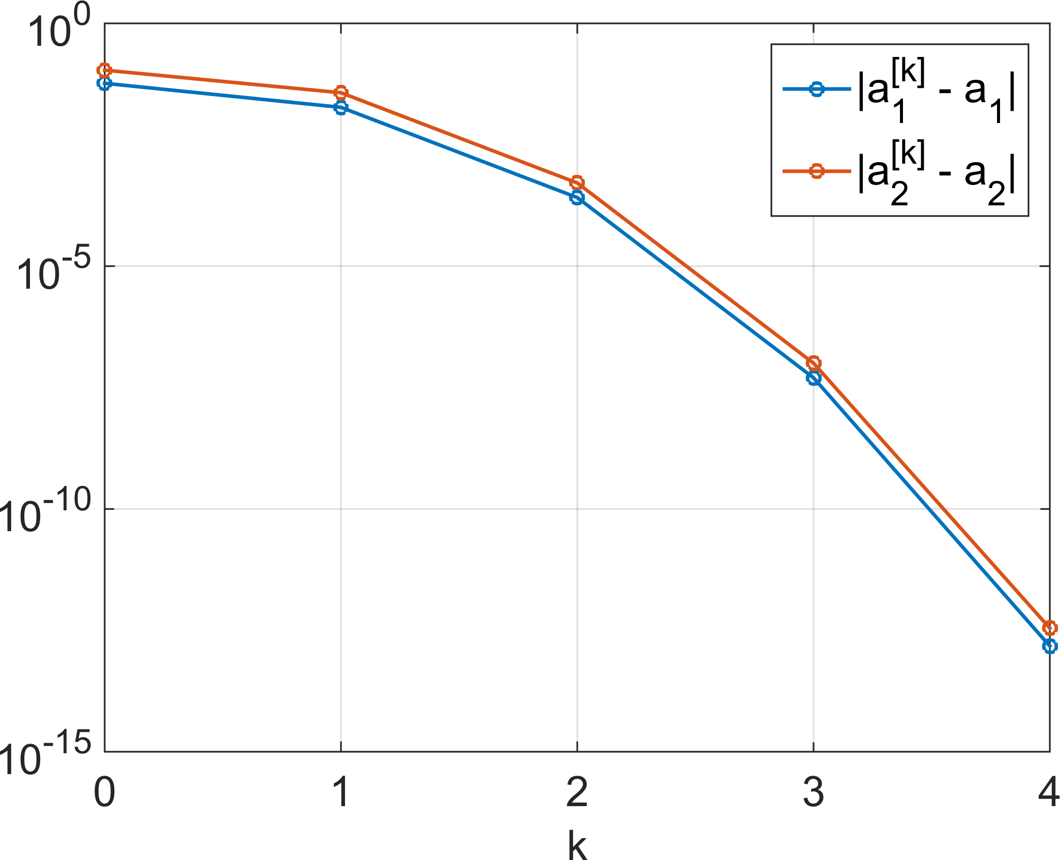
Figure 1: Error curves $\lvert a_{j}^{[k]}-a_{j}\rvert$ in Algorithm 4.8 applied to the sets $E$ in Example 4.10 (ii) (left) and (iii) (right). Missing dots mean that the error is exactly zero.

Example 4.11.

As a numerical experiment, we considered $500$ examples with random endpoints generating $5$ and $10$ intervals, respectively. In most cases, Algorithm 4.8 converged in $4$ or $5$ steps, and in all cases in at most $7$ steps.

5 The Conformal Map for Several Intervals

Let $E$ be the union of $\ell$ disjoint real intervals given in (4.1). The logarithmic capacity $\operatorname{cap}(E)$, the exponents $m_{1},\ldots,m_{\ell}$ and the centers $a_{1},\ldots,a_{\ell}$ of the canonical domain $L^{\operatorname{c}}$ have been obtained in Section 4. Next, we address the computation of the conformal map $\Phi:E^{\operatorname{c}}\to L^{\operatorname{c}}$.

For the computation of $\Phi(z)$ for real $z$, we need the following notation. The set $\mathbb{R}\setminus E$ consists of $\ell+1$ open intervals, denoted by $\mathbb{R}\setminus E=I_{0}\cup\ldots\cup I_{\ell}$, see (4.2). By [18, Thm. 2.1 (iv)], the set $\mathbb{R}\setminus L$ consists of $\ell+1$ open intervals

$$J_{0}=]-\infty,c_{1}[,\quad J_{k}=]c_{2k},c_{2k+1}[\quad\text{for }k=1,\ldots,\ell-1,\quad J_{\ell}=]c_{2\ell},\infty[,$$ (5.1)

where

$$\Phi(I_{k})=J_{k},\quad k=0,\ldots,\ell,$$ (5.2)

and $\Phi$ is strictly increasing on $\mathbb{R}\setminus E$. In particular, $\Phi(b_{j})=c_{j}\in\partial L$, $j=1,\ldots,2\ell$, and

$$-\infty<c_{1}<a_{1}<c_{2}<c_{3}<a_{2}<c_{4}<c_{5}<a_{3}<\ldots<c_{2\ell}<+\infty.$$ (5.3)

Our first result extends the identity $g_{E}(z)=g_{L}(\Phi(z))$, see (3.4), to the complex Green’s functions.

Theorem 5.1.

Let $E$ be as in (4.1) and $I_{0},\ldots,I_{\ell}$ be as in (4.2), then the following hold.

1. For $z\in\mathbb{C}\setminus]-\infty,b_{2\ell}]$,

   $$\sum_{j=1}^{\ell}m_{j}\log(\Phi(z)-a_{j})-\log(\operatorname{cap}(E))=\int_{b_{2\ell}}^{z}\frac{R(\zeta)}{\sqrt{H(\zeta)}}\,{\operatorname{d}}\zeta$$ (5.4)

   with the principal branch of the logarithm and an integration path from $b_{2\ell}$ to $z$ that lies in $\mathbb{C}\setminus]-\infty,b_{2\ell}]$ except for its starting point.

2. For $z\in I_{k}$, $k=0,\ldots,\ell$,

   $$\sum_{j=1}^{\ell}m_{j}\log\lvert\Phi(z)-a_{j}\rvert-\log(\operatorname{cap}(E))=\int_{b}^{z}\frac{R(x)}{\sqrt{H(x)}}\,{\operatorname{d}}x,$$ (5.5)

   where $\log$ is the real logarithm, the integration is along the real line and $b\in\{b_{1},\ldots,b_{2\ell}\}$ is an endpoint of $I_{k}$.

Proof.

By (3.4), we have $g_{E}(z)=g_{L}(\Phi(z))$, where $g_{L}$ is given by (3.1). By (3.9),

$$2\partial_{z}g_{E}(z)=\sum_{j=1}^{\ell}m_{j}\frac{\Phi^{\prime}(z)}{\Phi(z)-a_{j}},\quad z\in\mathbb{C}\setminus E,$$ (5.6)

and by Theorem 4.2 (ii) and (2.2), $2\partial_{z}g_{E}(z)=R(z)/\sqrt{H(z)}$.

(i) For $z\in\mathbb{C}\setminus]-\infty,b_{2\ell}]$, we integrate (5.6) along a path from $b_{2\ell}$ to $z$ that lies in the simply connected domain $\mathbb{C}\setminus]-\infty,b_{2\ell}]$ (except for the initial point $b_{2\ell}$) and obtain

$$\int_{b_{2\ell}}^{z}\frac{R(\zeta)}{\sqrt{H(\zeta)}}\,{\operatorname{d}}\zeta =\int_{b_{2\ell}}^{z}2\partial_{z}g_{E}(\zeta)\,{\operatorname{d}}\zeta=\sum_{j=1}^{\ell}m_{j}\int_{b_{2\ell}}^{z}\frac{\Phi^{\prime}(\zeta)}{\Phi(\zeta)-a_{j}}\,{\operatorname{d}}\zeta$$

$$=\sum_{j=1}^{\ell}m_{j}\log(\Phi(z)-a_{j})-\sum_{j=1}^{\ell}m_{j}\log(\Phi(b_{2\ell})-a_{j})$$

with the principal branch of the logarithm. Since $\Phi(b_{2\ell})\in\partial L$, we have $g_{L}(\Phi(b_{2\ell}))=0$. Together with $\Phi(b_{2\ell})>a_{j}$ for $j=1,\ldots,\ell$ and (3.1), this implies

$$\sum_{j=1}^{\ell}m_{j}\log(\Phi(b_{2\ell})-a_{j})=\sum_{j=1}^{\ell}m_{j}\log\lvert\Phi(b_{2\ell})-a_{j}\rvert=\log(\operatorname{cap}(E)).$$ (5.7)

This completes the proof of (i).

(ii) Let $k\in\{0,\ldots,\ell\}$. For $z\in I_{k}$, we integrate (5.6) from one endpoint $b\in\{b_{1},\ldots,b_{2k}\}$ of $I_{k}$ to $z$ along the real line. Similarly to (i), we have

$$\int_{b}^{z}\frac{R(x)}{\sqrt{H(x)}}\,{\operatorname{d}}x=\sum_{j=1}^{\ell}m_{j}\int_{b}^{z}\frac{\Phi^{\prime}(x)}{\Phi(x)-a_{j}}\,{\operatorname{d}}x=\sum_{j=1}^{\ell}m_{j}\log\lvert\Phi(z)-a_{j}\rvert-\log(\operatorname{cap}(E)).$$

Note that $\Phi(x)\neq a_{j}$ for all $x\in I_{k}$, which follows from (5.2) and (5.3). This completes the proof of (ii). ∎

Remark 5.2.

If we replace $b_{2\ell}$ by $b\in\{b_{2k},b_{2k+1}\}$ for some $k\in\{0,\ldots,\ell-1\}$ (where $b_{0}\coloneq b_{1}$) in Theorem 5.1 (i) then we obtain similarly to (5.7)

$$\sum_{j=1}^{\ell}m_{j}\log(\Phi(b)-a_{j})=\log(\operatorname{cap}(E))\pm{\operatorname{i}}\pi(m_{k+1}+\ldots+m_{\ell}),$$

since then $\Phi(b)<a_{j}$ for $j=k+1,\ldots,\ell$ and $\Phi(b)>a_{j}$ for $j=1,\ldots,k$. Therefore, for $z\in\mathbb{C}\setminus\mathbb{R}$, $\Phi(z)$ satisfies

$$\sum_{j=1}^{\ell}m_{j}\log(\Phi(z)-a_{j})-\log(\operatorname{cap}(E))\mp{\operatorname{i}}\pi(m_{k+1}+\ldots+m_{\ell})=\int_{b}^{z}\frac{R(\zeta)}{\sqrt{H(\zeta)}}\,{\operatorname{d}}\zeta,$$

where the sign of “$\mp$” is “$-$” if $\operatorname{Im}(z)>0$ and “$+$” if $\operatorname{Im}(z)<0$. This shows that, for $b\in\{b_{2k},b_{2k+1}\}$, the complex Green’s function of $E^{\operatorname{c}}$ satisfies

$$\int_{b}^{z}\frac{R(\zeta)}{\sqrt{H(\zeta)}}\,{\operatorname{d}}\zeta=\int_{b_{2\ell}}^{z}\frac{R(\zeta)}{\sqrt{H(\zeta)}}\,{\operatorname{d}}\zeta\mp{\operatorname{i}}\pi(m_{k+1}+\ldots+m_{\ell}),\quad z\in\mathbb{C}\setminus\mathbb{R}.$$ (5.8)

This shows that for the real Green’s function of $E^{\operatorname{c}}$, see Theorem 4.2 (ii), the point $b$ can indeed be any of the endpoints $\{b_{1},\ldots,b_{2\ell}\}$.

Equations (5.4) and (5.5) in Theorem 5.1 can be solved numerically in order to obtain the value $\Phi(z)$. More precisely, if $z\in\mathbb{C}\setminus\mathbb{R}$, we solve

$$F_{1}(w)\coloneq\sum_{j=1}^{\ell}m_{j}\log(w-a_{j})-\log(\operatorname{cap}(E))=\int_{b_{2\ell}}^{z}\frac{R(\zeta)}{\sqrt{H(\zeta)}}\,{\operatorname{d}}\zeta,\quad w\in\mathbb{C}\setminus\mathbb{R},$$ (5.9)

with the principal branch of the logarithm, and, if $z\in I_{k}$, $k=0,\ldots,\ell$, we solve

$$F_{2}(w)\coloneq\sum_{j=1}^{\ell}m_{j}\log\lvert w-a_{j}\rvert-\log(\operatorname{cap}(E))=\int_{b}^{z}\frac{R(x)}{\sqrt{H(x)}}\,{\operatorname{d}}x,\quad w\in\mathbb{R}\setminus L,$$ (5.10)

with real logarithms, and where $b\in\{b_{1},\ldots,b_{2\ell}\}$ is an endpoint of $I_{k}$. By Theorem 5.1, $w=\Phi(z)$ is one solution, and we discuss its uniqueness next.

Theorem 5.3.

Let $E$ be as in (4.1) and $I_{0},\ldots,I_{\ell}$ and $J_{0},\ldots,J_{\ell}$ be as in (4.2) and (5.1), respectively, then the following holds.

1. For $z\in\mathbb{C}\setminus\mathbb{R}$, equation (5.9) has the unique solution $w=\Phi(z)$.

2. For $z\in\mathbb{R}\setminus E$, equation (5.10) has the unique solution $w=\Phi(z)$ for $w$ restricted to a suitable interval depending on $z$:

   1. If $z\in I_{0}$ then $w\in J_{0}$.

   2. If $z\in I_{\ell}$ then $w\in J_{\ell}$.

   3. If $z\in I_{k}$, $k=1,\ldots,\ell-1$, then

      • if $z\in]b_{2k},z_{k}[$ then $w\in]c_{2k},w_{k}[$,

      • if $z=z_{k}$ then $w=w_{k}$,

      • if $z\in]z_{k},b_{2k+1}[$ then $w\in]w_{k},c_{2k+1}[$,

      where $z_{1},\ldots,z_{\ell-1}$ are the critical points of $g_{E}$, compare Corollary 4.3 (ii), and $w_{1},\ldots,w_{\ell-1}$ are the critical points of $g_{L}$, compare (4.21).

Proof.

(i) In order to show that (5.9) has a unique solution $w$, we consider the mapping properties of the function $F_{1}$ in the upper half-plane $\mathbb{H}=\{w\in\mathbb{C}:\operatorname{Im}(w)>0\}$. Since $F_{1}^{\prime}(w)=\sum_{j=1}^{\ell}m_{j}/(w-a_{j})$, the critical points of $F_{1}$ are the critical points $w_{1},\ldots,w_{\ell-1}$ of $g_{L}$, compare (3.2), which are real by (4.21), hence $F_{1}$ is conformal in $\mathbb{H}$. The function $F_{1}$ can be written as

$$F_{1}(w)=\sum_{j=1}^{\ell}m_{j}\log\lvert w-a_{j}\rvert-\log(\operatorname{cap}(E))+{\operatorname{i}}\sum_{j=1}^{\ell}m_{j}\arg(w-a_{j})=g_{L}(w)+{\operatorname{i}}h_{L}(w),$$

with the principal branch of the argument. Thus $\arg(w-a_{j})\in]0,\pi[$ for $\operatorname{Im}(w)>0$ and $F_{1}$ maps $\mathbb{H}$ into the strip $\{\zeta\in\mathbb{C}:0<\operatorname{Im}(\zeta)<\pi\}$. Let us consider the behaviour of $F_{1}$ on the real line. The function $h_{L}$ has the values

$$h_{L}(w)=\begin{cases}0,&w>a_{\ell},\\ (m_{k+1}+\ldots+m_{\ell})\pi,&a_{k}<w<a_{k+1},\\ \pi,&w<a_{1},\end{cases}$$

and $g_{L}$ satisfies $\lim_{w\to\pm\infty}g_{L}(w)=+\infty$ and $\lim_{w\to a_{j}}g_{L}(w)=-\infty$. Moreover, $g_{L}$ has the critical points $w_{1},\ldots,w_{\ell-1}$ which satisfy (4.21) and $g_{L}(w_{k})>0$ for $k=1,\ldots,\ell-1$. Therefore,

$$F_{1}(]a_{\ell},+\infty[) =]-\infty,+\infty[,$$

$$F_{1}(]a_{k},w_{k}]) =F_{1}([w_{k},a_{k+1}[)=]-\infty,g_{L}(w_{k})]+{\operatorname{i}}(m_{k+1}+\ldots+m_{\ell})\pi,$$

$$F_{1}(]-\infty,a_{1}[) =]-\infty,+\infty[+{\operatorname{i}}\pi.$$

This shows that $F_{1}$ maps the upper half-plane $\mathbb{H}$ conformally into the strip with slits

$$S=\{\zeta\in\mathbb{C}:0<\operatorname{Im}(\zeta)<\pi\}\setminus\bigcup_{k=1}^{\ell-1}\Bigl{(}]-\infty,g_{L}(w_{k})]+{\operatorname{i}}(m_{k+1}+\ldots+m_{\ell})\pi\Bigr{)}.$$

By distinguishing the two sides of the slits, $F_{1}$ maps $\partial\mathbb{H}$ bijectively onto the boundary of $S$ and thus is univalent in $\mathbb{H}$. Since $F_{1}(w)=\overline{F_{1}(\overline{w})}$ for all $w\in\mathbb{C}\setminus\mathbb{R}$, the function $F_{1}$ is univalent in $\mathbb{C}\setminus\mathbb{R}$. Together with Theorem 5.1, this shows that $w=\Phi(z)$ is the unique solution of (5.9).

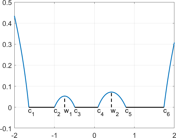
Figure 2: Illustration of the proof of Theorem 5.3 (ii): The graph of the function $F_{2}(w)=g_{L}(w)$ for $w\in\mathbb{R}\setminus L$.

(ii) The proof relies on the piece-wise monotonicity of $F_{2}$ in $\mathbb{R}\setminus L$. Fix $k\in\{0,\ldots,\ell\}$ and $z\in I_{k}$. Then $\Phi(z)\in J_{k}$, see (5.2), and we solve (5.10) for $w\in J_{k}$. The function $F_{2}:J_{k}\to\mathbb{R}$ is real analytic with derivative

$$F_{2}^{\prime}(w)=\sum_{j=1}^{\ell}\frac{m_{j}}{w-a_{j}}.$$

For $k=1,\ldots,\ell-1$, the function $F_{2}$ satisfies $F_{2}(w)>0$ for $w\in J_{k}=]c_{2k},c_{2k+1}[$ and $F_{2}(c_{2k})=F_{2}(c_{2k+1})=0$, and $F_{2}$ has a unique critical point $w_{k}$ with $c_{2k}<w_{k}<c_{2k+1}$. Therefore, $F_{2}$ is strictly increasing on $[c_{2k},w_{k}]$ and strictly decreasing on $[w_{k},c_{2k+1}]$; see Figure 2 for an illustration. Since $\Phi(z_{k})=w_{k}$, where $z_{k}$ is the critical point of $g_{E}$ in $I_{k}$, and taking into account the mapping properties of $\Phi$ in [18, Thm. 2.1 (v)], this leads to the following statement. If $b_{2k}<z<z_{k}$ then (5.10) has the unique solution $w=\Phi(z)$ with $c_{2k}<w<w_{k}$. If $z_{k}<z<b_{2k+1}$ then (5.10) has the unique solution $w=\Phi(z)$ with $w_{k}<w<c_{2k+1}$. Since $F_{2}^{\prime}(w)<0$ for $w\in J_{0}$ and $F_{2}^{\prime}(w)>0$ for $w\in J_{\ell}$, in both cases, equation (5.10) has the unique solution $w=\Phi(z)$. This completes the proof of (ii). ∎

Remark 5.4.

The points $c_{1},\ldots,c_{2\ell}$ in (5.1) are the real zeros of the Green’s function $g_{L}$ in (3.1) and can be computed, e.g., with bisection or Newton’s method.

Next, we discuss the numerical solution of equations (5.9) and (5.10). The derivatives of both functions $F_{1}$ and $F_{2}$ are $\sum_{j=1}^{\ell}m_{j}/(w-a_{j})$. We solve (5.9) and (5.10) with the damped Newton iteration

$$w^{[k+1]}=w^{[k]}-d\frac{F_{i}(w^{[k]})-\int_{b}^{z}\frac{R(\zeta)}{\sqrt{H(\zeta)}}\,{\operatorname{d}}\zeta}{\sum_{j=1}^{\ell}\frac{m_{j}}{w^{[k]}-a_{j}}},\quad k=0,1,2,\ldots,$$ (5.11)

where we use the damping parameter $d=1,2^{-1},2^{-2},\ldots,2^{-10}$. In view of Theorem 5.3, we choose the initial point $w^{[0]}$ for the individual cases as follows. For given $z\in\mathbb{C}\setminus\mathbb{R}$, we solve (5.9) with $w^{[0]}=z$. For $z\in\mathbb{R}\setminus E$, we solve (5.10) with

$$w^{[0]}=\begin{cases}z&\text{if }z\in I_{0}\text{ or }z\in I_{\ell},\\ c_{2k}+\frac{z-b_{2k}}{z_{k}-b_{2k}}(w_{k}-c_{2k})&\text{if }z\in]b_{2k},z_{k}[,\\ w_{k}+\frac{z-z_{k}}{b_{2k+1}-z_{k}}(c_{2k+1}-w_{k})&\text{if }z\in]z_{k},b_{2k+1}[.\end{cases}$$

Note that for $z\in]b_{2k},z_{k}[$ or $z\in]z_{k},b_{2k+1}[$ one could also use only bisection to solve (5.10). However, the Newton iteration typically converges faster than bisection.

Example 5.5.

Let $E=[-1,-0.3]\cup[0.1,1]$ be as in Example 4.7, where we already computed all parameters of the set $L$. The values $\Phi(z)$ of the conformal map for $z\in\mathbb{C}\setminus E$ are obtained as described above. Figure 3 shows a grid and its image under $\Phi$ as well as the set $E$ and the corresponding set $L$.

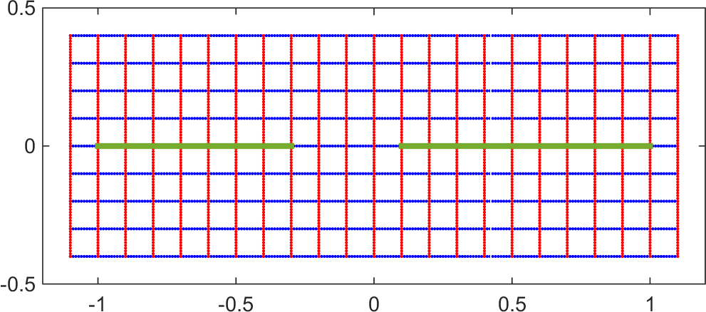
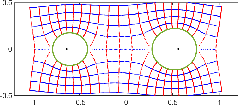
Figure 3: Left: Set $E=[-1,-0.3]\cup[0.1,1]$ in Example 5.5 with a grid. Right: $\partial L$ (green curves), $a_{1},a_{2}$ (black dots) and the image of the grid under $\Phi$.

Example 5.6.

Let $E=[-2,-0.9]\cup[-0.7,0.2]\cup[0.5,2.2]$, i.e., $\ell=3$. Let us compute the parameters of the corresponding lemniscatic domain $L^{\operatorname{c}}$. First, we compute the coefficients of the polynomial $R$ with the help of (4.12). Using Theorem 4.4, we obtain the exponents $m_{1}=0.3601$, $m_{2}=0.1772$, $m_{3}=0.4627$ (all values rounded to four decimal places). The capacity $\operatorname{cap}(E)=1.0458$ is derived from Corollary 4.3 (iv).

Next, we calculate $a_{1},a_{2},a_{3}$ in two ways: first, by solving the non-linear system of equations (3.14), and second, using Algorithm 4.8. In both variants, we obtain $a_{1}=-1.4101$, $a_{2}=-0.1950$, $a_{3}=1.3896$, where the values agree up to seven digits. Algorithm 4.8 converges in $4$ steps. The set $L$ is shown in Figure 4 (right), which also shows the values of $\Phi$ on a grid.

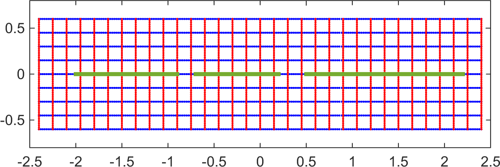
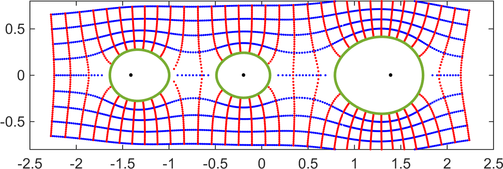
Figure 4: Left: Set $E=[-2,-0.9]\cup[-0.7,0.2]\cup[0.5,2.2]$ in Example 5.6 with a grid. Right: $\partial L$ (green curves), $a_{1},a_{2},a_{3}$ (black dots) and the image of the grid under $\Phi$.

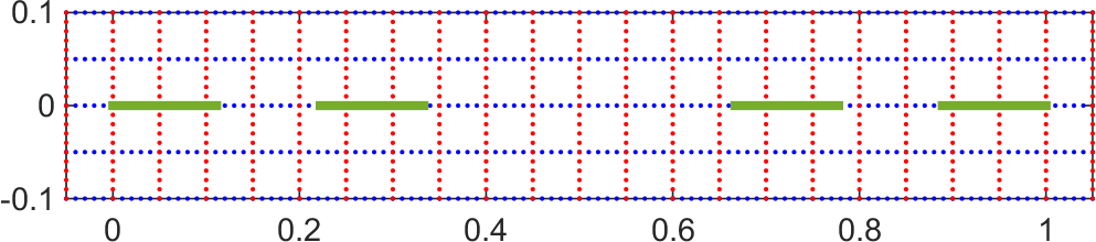
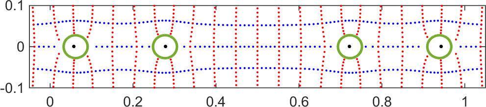
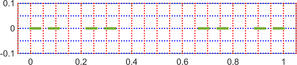
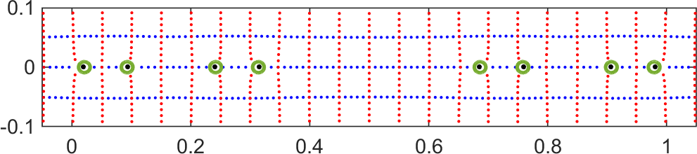
Figure 5: Panels 1 and 3: Sets $E_{2}$ and $E_{3}$ from the construction of the Cantor middle third set (see Example 5.7) with a grid. Panels 2 and 4: Corresponding sets $L$ (with $\partial L$ in green), centers $a_{j}$ (black dots), and image of the grid under $\Phi$.

Example 5.7.

The classical Cantor middle third set is defined by

$$E=\bigcap_{k=0}^{\infty}E_{k},\quad\text{where }E_{0}=[0,1],\quad E_{k+1}=\frac{1}{3}E_{k}\cup\left(\frac{2}{3}+\frac{1}{3}E_{k}\right),\quad k\geq 0.$$

We consider the two sets $E_{2}$ and $E_{3}$ which consist of $4$ and $8$ intervals, respectively. The logarithmic capacities, numerically computed with (4.17), are

$$\operatorname{cap}(E_{2})=0.228430704425168\quad\text{and}\quad\operatorname{cap}(E_{3})=0.224752818755217$$

and agree in the first 12 digits with the values found in [10, Ex. 4.13]. We compute the centers with Algorithm 4.8, which numerically converges in $2$ steps for $E_{2}$ and in $3$ steps for $E_{3}$. Figure 5 shows the sets $E_{2},E_{3}$, the corresponding sets $L$ and the conformal map $\Phi$, evaluated numerically on a grid.

Remark 5.8.

In all previous examples of sets $E=E_{1}\cup\ldots\cup E_{\ell}$ consisting of $\ell$ real intervals, the centers $a_{j}$ were located in the intervals $E_{j}$. This is not true in general, as the example $E=[-1,1]\cup[1.2,1.4]$ shows, where the computed centers of $L$ are $a_{1}=-0.0677\ldots\in E_{1}$, $a_{2}=1.0862\ldots\notin E_{2}$.

Appendix A Proofs

Proof of Corollary 3.3.

Let $\alpha$ be the coefficient of $z^{-2}$ in the Laurent series of $\partial_{z}g_{E}$ as in Lemma 3.1. We prove that $\alpha=-p_{n-1}/(np_{n})$. Let $\mathcal{R}:\Omega^{\operatorname{c}}\to\{w\in\widehat{\mathbb{C}}:\lvert w\rvert>1\}$ with $\mathcal{R}(\infty)=\infty$ and $\mathcal{R}^{\prime}(\infty)>0$ be the exterior Riemann map of $\Omega$. Its Laurent series at infinity has the form $\mathcal{R}(z)=d_{1}z+d_{0}+\mathcal{O}(z^{-1})$. By [17, Eq. (3.7)],

$$2\partial_{z}g_{E}(z)=\frac{1}{n}\frac{(\mathcal{R}\circ P)^{\prime}(z)}{(\mathcal{R}\circ P)(z)}.$$

Since $n\geq 2$, we have

$$(\mathcal{R}\circ P)(z) =d_{1}(p_{n}z^{n}+p_{n-1}z^{n-1}+\mathcal{O}(z^{n-2})),$$

$$(\mathcal{R}\circ P)^{\prime}(z) =d_{1}(np_{n}z^{n-1}+(n-1)p_{n-1}z^{n-2}+\mathcal{O}(z^{n-3})),$$

and hence

$$2\partial_{z}g_{E}(z) =\frac{1}{n}\frac{np_{n}z^{n-1}+(n-1)p_{n-1}z^{n-2}+\mathcal{O}(z^{n-3})}{p_{n}z^{n}+p_{n-1}z^{n-1}+\mathcal{O}(z^{n-2})}$$

$$=\frac{z^{-1}+\frac{n-1}{n}\frac{p_{n-1}}{p_{n}}z^{-2}+\mathcal{O}(z^{-3})}{1+\frac{p_{n-1}}{p_{n}}z^{-1}+\mathcal{O}(z^{-2})}.$$

Using $1/(1+z)=1-z+\mathcal{O}(z^{2})$ for $\lvert z\rvert<1$, we obtain

$$2\partial_{z}g_{E}(z) =\Bigl{(}z^{-1}+\frac{n-1}{n}\frac{p_{n-1}}{p_{n}}z^{-2}+\mathcal{O}(z^{-3})\Bigr{)}\Bigl{(}1-\frac{p_{n-1}}{p_{n}}z^{-1}+\mathcal{O}(z^{-2})\Bigr{)}$$

$$=z^{-1}-\frac{p_{n-1}}{np_{n}}z^{-2}+\mathcal{O}(z^{-3})$$

and (3.11) follows by applying Theorem 3.2. ∎

Proof of Theorem 4.4.

We use the integral representation (2.3). The Green’s function $g_{E}$ is given by (4.9), hence the Wirtinger derivative of $g_{E}$ is

$$2\partial_{z}g_{E}(z)=\frac{R(z)}{\sqrt{H(z)}}$$

by (2.2), and therefore

$$m_{j}=\frac{1}{2\pi{\operatorname{i}}}\int_{\gamma_{j}}\frac{R(z)}{\sqrt{H(z)}}\,{\operatorname{d}}z,\quad j=1,\ldots,\ell,$$

where $\gamma_{j}$ is a (smooth) closed curve in $\mathbb{C}\setminus E$ with $\operatorname{wind}(\gamma_{j};z)=\delta_{jk}$ for $z\in E_{k}$. Since $R(z)/\sqrt{H(z)}$ is analytic in $\mathbb{C}\setminus E$ with branch cuts along the intervals $E_{j}$ (compare Lemma 4.1) and has singularities at the endpoints of the intervals, i.e., at $b_{1},\ldots,b_{2n}$, we can deform $\gamma_{j}$ as follows without changing the value of the integral:

$$m_{j} =\frac{1}{2\pi{\operatorname{i}}}\int_{b_{2j-1}+\varepsilon}^{b_{2j}-\varepsilon}\frac{R(x)}{\sqrt{H(x-0{\operatorname{i}})}}\,{\operatorname{d}}x-\frac{1}{2\pi{\operatorname{i}}}\int_{b_{2j-1}+\varepsilon}^{b_{2j}-\varepsilon}\frac{R(x)}{\sqrt{H(x+0{\operatorname{i}})}}\,{\operatorname{d}}x$$

$$\phantom{=}+\int_{C_{1}}\frac{R(z)}{\sqrt{H(z)}}\,{\operatorname{d}}z+\int_{C_{2}}\frac{R(z)}{\sqrt{H(z)}}\,{\operatorname{d}}z,$$

where $\sqrt{H(x\pm 0{\operatorname{i}})}=\lim_{y\searrow 0}\sqrt{H(x\pm{\operatorname{i}}y)}$ denote the values of $\sqrt{H(z)}$ on the two rims of the branch cut $[b_{2j-1},b_{2j}]$, and where $C_{1}$, $C_{2}$ are circular arcs parametrized by $b_{2j-1}+\varepsilon{\operatorname{e}}^{{\operatorname{i}}t}$, $0\leq t\leq 2\pi$, and $b_{2j}+\varepsilon{\operatorname{e}}^{{\operatorname{i}}t}$, $-\pi\leq t\leq\pi$, respectively. The integrals over the circular arcs vanish for $\varepsilon\to 0$, since

$$\left\lvert\int_{C_{k}}\frac{R(z)}{\sqrt{H(z)}}\,{\operatorname{d}}z\right\rvert\leq L(C_{k})\max_{z\in C_{k}}\frac{\lvert R(z)\rvert}{\sqrt{\lvert H(z)\rvert}}\leq 2\pi\varepsilon\frac{M}{\sqrt{\varepsilon}},$$

which yields

$$m_{j}=\frac{1}{2\pi{\operatorname{i}}}\int_{b_{2j-1}}^{b_{2j}}\Biggl{(}\frac{R(x)}{\sqrt{H(x-0{\operatorname{i}})}}-\frac{R(x)}{\sqrt{H(x+0{\operatorname{i}})}}\Biggr{)}\,{\operatorname{d}}x.$$

By Lemma 4.1 and together with (4.14), we obtain for $x\in]b_{2j-1},b_{2j}[$, $j=1,\ldots,\ell$,

$$\frac{R(x)}{\sqrt{H(x-0{\operatorname{i}})}}-\frac{R(x)}{\sqrt{H(x+0{\operatorname{i}})}}=\frac{(-1)^{\ell-j}\lvert R(x)\rvert}{\sqrt{\lvert H(x)\rvert}}\left(\frac{1}{-{\operatorname{i}}(-1)^{\ell-j}}-\frac{1}{{\operatorname{i}}(-1)^{\ell-j}}\right)=2{\operatorname{i}}\frac{\lvert R(x)\rvert}{\sqrt{\lvert H(x)\rvert}},$$

which is also stated in [13, Proof of Lem. 2.2 (a)]. This shows

$$m_{j}=\frac{1}{\pi}\int_{b_{2j-1}}^{b_{2j}}\frac{\lvert R(x)\rvert}{\sqrt{\lvert H(x)\rvert}}\,{\operatorname{d}}x$$

and the assertion now follows together with (4.11). ∎

References

[1]A. B. Bogatyrev and O. A. Grigoriev, Closed formula for the capacity
of several aligned segments, Proc. Steklov Inst. Math., 298 (2017),
pp. 60–67.
[2]V. Dubinin and D. Karp, Two-sided bounds for the logarithmic
capacity of multiple intervals, J. Anal. Math., 113 (2011), pp. 227–239.
[3]M. Embree and L. N. Trefethen, Green’s functions for multiply
connected domains via conformal mapping, SIAM Review, 41 (1999),
pp. 745–761.
[4]J. B. Garnett and D. E. Marshall, Harmonic measure, vol. 2 of New
Mathematical Monographs, Cambridge University Press, Cambridge, 2005.
[5]H. Grunsky, Über konforme Abbildungen, die gewisse
Gebietsfunktionen in elementare Funktionen transformieren. I, Math.
Z., 67 (1957), pp. 129–132.
[6], Über konforme
Abbildungen, die gewisse Gebietsfunktionen in elementare Funktionen
transformieren. II, Math. Z., 67 (1957), pp. 223–228.
[7], Lectures on theory
of functions in multiply connected domains, Vandenhoeck & Ruprecht,
Göttingen, 1978.
[8]J. A. Jenkins, On a canonical conformal mapping of J. L.
Walsh, Trans. Amer. Math. Soc., 88 (1958), pp. 207–213.
[9]H. J. Landau, On canonical conformal maps of multiply connected
domains, Trans. Amer. Math. Soc., 99 (1961), pp. 1–20.
[10]J. Liesen, O. Sète, and M. M. S. Nasser, Fast and accurate
computation of the logarithmic capacity of compact sets, Comput. Methods
Funct. Theory, 17 (2017), pp. 689–713.
[11]G. Mantica, Computing the equilibrium measure of a system of
intervals converging to a cantor set, Dolomites Research Notes on
Approximation, 6 (2013), pp. 51–61.
[12]M. M. S. Nasser, J. Liesen, and O. Sète, Numerical computation of
the conformal map onto lemniscatic domains, Comput. Methods Funct. Theory,
16 (2016), pp. 609–635.
[14], On
Bernstein-Szegő orthogonal polynomials on several intervals. II.
Orthogonal polynomials with periodic recurrence coefficients, J. Approx.
Theory, 64 (1991), pp. 123–161.
[15], Orthogonal and
extremal polynomials on several intervals, J. Comput. Appl. Math., 48
(1993), pp. 187–205.
[16]T. Ransford, Potential theory in the complex plane, vol. 28 of
London Mathematical Society Student Texts, Cambridge University Press,
Cambridge, 1995.
[17]K. Schiefermayr and O. Sète, Walsh’s conformal map onto
lemniscatic domains for polynomial pre-images I, Comput. Methods Funct.
Theory, 23 (2023), pp. 489–511.
[18]K. Schiefermayr and O. Sète, Walsh’s conformal map onto
lemniscatic domains for polynomial pre-images II, Comput. Methods Funct.
Theory, (2023).
(Online first).
[19]O. Sète and J. Liesen, On conformal maps from multiply connected
domains onto lemniscatic domains, Electron. Trans. Numer. Anal., 45 (2016),
pp. 1–15.
[20]O. Sète and J. Liesen, Properties and examples of Faber-Walsh
polynomials, Comput. Methods Funct. Theory, 17 (2017), pp. 151–177.
[21]J. Shen, G. Strang, and A. J. Wathen, The potential theory of
several intervals and its applications, Appl. Math. Optim., 44 (2001),
pp. 67–85.
[22]P. K. Suetin, Series of Faber polynomials, vol. 1 of Analytical
Methods and Special Functions, Gordon and Breach Science Publishers,
Amsterdam, 1998.
[23]J. L. Walsh, On the conformal mapping of multiply connected
regions, Trans. Amer. Math. Soc., 82 (1956), pp. 128–146.
[24], A generalization of
Faber’s polynomials, Math. Ann., 136 (1958), pp. 23–33.
[25], Interpolation and
approximation by rational functions in the complex domain, Fifth edition.
American Mathematical Society Colloquium Publications, Vol. XX, American
Mathematical Society, Providence, R.I., 1969.
[26]J. L. Walsh, Selected papers, Springer-Verlag, New York, 2000.
With brief biographical sketches of Walsh by W. E. Sewell, D. V.
Widder and Morris Marden and commentaries by Q. I. Rahman, P. M. Gauthier,
Dieter Gaier, Walter Schempp and the editors, Edited by Theodore J. Rivlin
and Edward B. Saff.
[27]H. Widom, Extremal polynomials associated with a system of curves in
the complex plane, Advances in Math., 3 (1969), pp. 127–232.