Can Tree Based Approaches Surpass Deep Learning in Anomaly Detection? A Benchmarking Study

Abstract

Detection of anomalous situations for complex mission-critical systems holds paramount importance when their service continuity needs to be ensured. A major challenge in detecting anomalies from the operational data arises due to the imbalanced class distribution problem since the anomalies are supposed to be rare events. This paper evaluates a diverse array of machine learning-based anomaly detection algorithms through a comprehensive benchmark study.

The paper contributes significantly by conducting an unbiased comparison of various anomaly detection algorithms, spanning classical machine learning including various tree-based approaches to deep learning and outlier detection methods. The inclusion of 104 publicly available and a few proprietary industrial systems datasets enhances the diversity of the study, allowing for a more realistic evaluation of algorithm performance and emphasizing the importance of adaptability to real-world scenarios.

The paper dispels the deep learning myth, demonstrating that though powerful, deep learning is not a universal solution in this case. We observed that recently proposed tree-based evolutionary algorithms outperform in many scenarios. We noticed that tree-based approaches catch a singleton anomaly in a dataset where deep learning methods fail. On the other hand, classical SVM performs the best on datasets with more than 10% anomalies, implying that such scenarios can be best modeled as a classification problem rather than anomaly detection. To our knowledge, such a study on a large number of state-of-the-art algorithms using diverse data sets, with the objective of guiding researchers and practitioners in making informed algorithmic choices, has not been attempted earlier.

1 Introduction

Identification of anomalies or outliers has wide applicability, from fraud detection in financial transactions, security vulnerability identification, performance bottleneck analysis, fault detection in industrial processes, system reliability evaluation and so on. Nowadays, anomaly detection methods primarily use operational data of the system under consideration and construct a machine learning (ML) model. A major challenge in building an effective ML model for anomaly detection is that the presence of anomalies in the dataset is rare. In streamlined industrial systems, a minority class instance (an anomalous condition) may occur once in thousands or millions of execution instances, causing a severe class imbalance for a classification-based ML model. This is a critical concern as, detecting anomalous conditions holds greater significance, making classification errors in this class more impactful than those in the majority class.

In recent years, deep neural networks have garnered significant attention in the anomaly detection field due to their impressive ability to automatically uncover complex data patterns and features. At the same time, tree-based ensemble methods such as Random Forests[3], and Isolation Forests [34] have been comparatively less discussed in the anomaly detection community. LinkedIn is one such example where an Isolation Forest based method detects various forms of abuse[50]. Despite their efficacy in various domains, tree-based approaches have often operated in the shadow of deep learning models, prompting us to revisit and reevaluate the efficacy of various machine learning methods for anomaly detection. In this paper, we have conducted an unbiased and comprehensive comparison of various anomaly detection algorithms, encompassing a wide spectrum of methodologies. The summary of our findings is depicted in Figure  1.

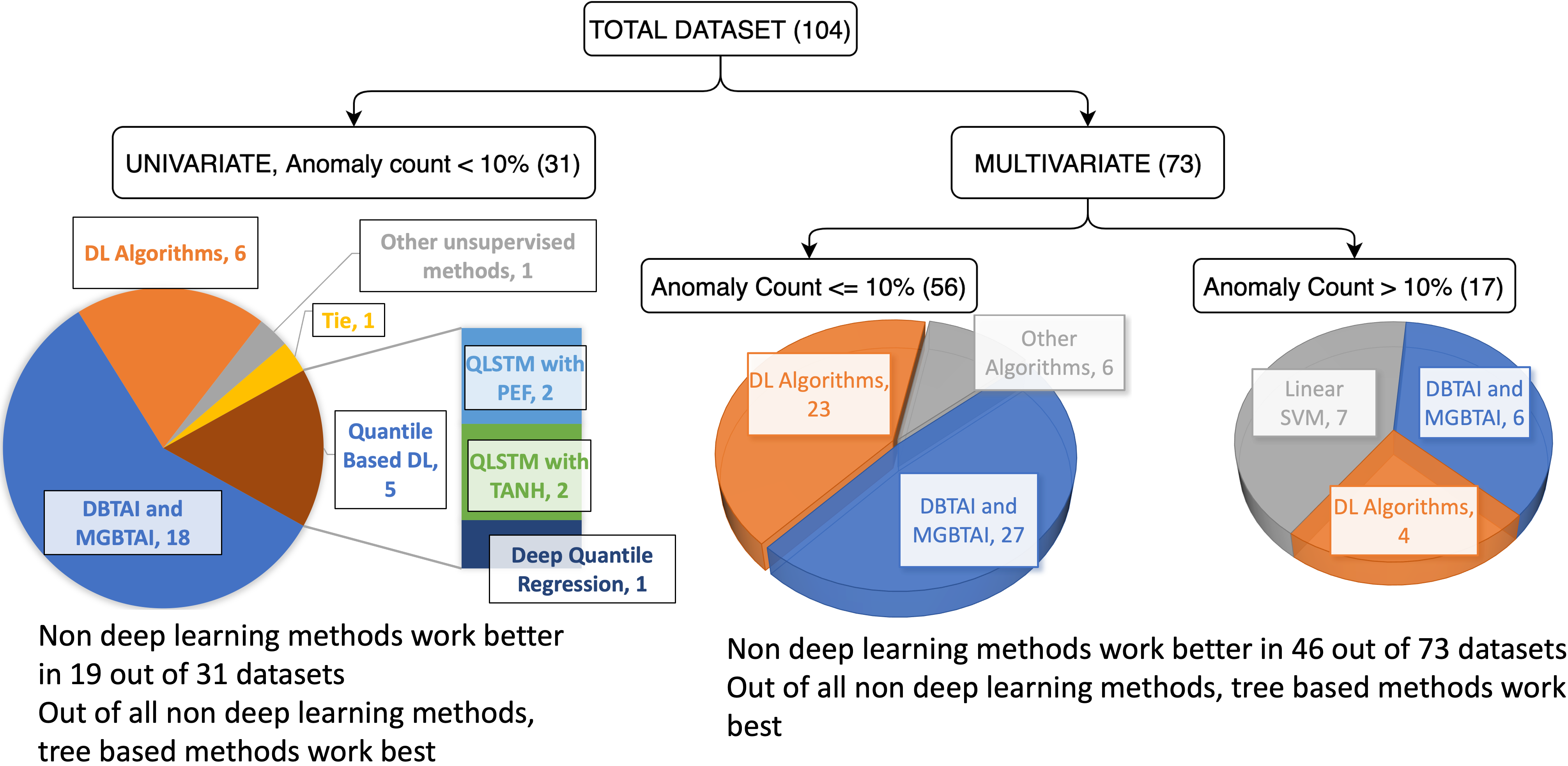
Figure 1: Comparison of algorithms. The Algorithm obtaining the highest Recall has been given credit. In case the recall value is the same for two or more algorithms, the comparison is performed based on precision.

Our contributions are as follows:

1. Performance Evaluation: Our empirical study assesses a range of state-of-the-art (SOTA) machine learning algorithms namely local outlier factor[4], isolation forest[34], one-class SVM[26], auto-encoders[55], deep autoencoding gaussian mixture model[58], LSTM[27], quantile LSTM[43], deep quantile regression[49], elliptical envelope[42], DevNet[39], GAN[23], GNN[13], Binary tree-based algorithms (MGBTAI[45] and d-BTAI[46]), for their efficacy in detecting anomalies from a large class of public and proprietary industrial datasets. The side-by-side comparison applied on datasets from different domains helps validate the algorithms’ robustness and generalizability.

2. Generalizability of tree-based unsupervised approach: In this work, we observed that tree-based evolutionary algorithms reported remarkable adaptability where they excel in anomaly detection when there are rare as well as significant volumes of anomalies. We have enhanced the knee/elbow methods for these algorithms to determine thresholds which effectively identify the inflection point in anomaly score distributions.

3. Debunking the Deep Learning Myth: Our evaluation dispels the common misconception that deep learning is the panacea for anomaly detection. By evaluating a wide array of SOTA DL algorithms in the study, the research demonstrates that while deep learning is undoubtedly powerful, its performance may not consistently surpass that of other well-established methods.

4. Optimal Anomaly Detection Settings: Our experiment demonstrated that the presence of a high percentage of anomalies (such as in the multivariate datasets used in this study) pose a unique challenge for anomaly detection since an overwhelming abundance of anomalies can obscure the characteristics that distinguish them from normal data.We empirically observed that anomaly detection methods work well on datasets with less than 10% anomalies. We showed that with a smaller anomaly percentage, precision, recall, and the F1-score become more informative and reflective of a model’s true anomaly detection capabilities.

2 Literature Review

Data-driven anomaly detection has been extensively researched for more than a decade. The report by  [9] classified various types of anomalies and detection approaches before the prominence of machine learning based approaches. Subsequently several academic surveys have been conducted on deep learning based anomaly detection [8, 39].There have been surveys on domain specific anomaly detection such as deep learning based anomaly detection algorithms for images and videos [31, 35, 12], network traffic [51, 17], real-time data [24, 11, 36], urban traffice [14] and so on. In another recent survey, researchers have reviewed 52 algorithms and grouped them by statistics, density, distance, clustering, isolation, ensemble and so on [44]. While this body of work provides a rich landscape of anomaly detection techniques, they do not deep-dive any of these methods to understand the efficacies and limitations through empirical studies.

Existing anomaly detection systems have used a combination of statistical methods [56], machine learning algorithms[21, 2, 7, 13, 18, 37, 19], and domain-specific techniques.

Using industrial data, [33] demonstrated that supervised anomaly detection faces challenges with scarce anomaly labels, adapting to new machine classes, and complex machinery. Rule-based classifier methods may struggle with unseen patterns, and ensemble techniques have limitations in memory and high-dimensional data. Anomaly detection systems that rely on static thresholds struggle to adapt to dynamic data containing evolving patterns, resulting in high false positives and missed anomalies. To address these issues, there is a growing shift towards unsupervised and semi-supervised learning approaches. The work by  [31] observed that unsupervised anomaly detection can be computationally intensive, especially in high-dimensional datasets. Jacob and Tatbul [29] delved into explainable anomaly detection in time series using real-world data, yet deep learning-based time-series anomaly detection models were not thoroughly explored well enough.

Density-based methods struggle with varying data densities, and profile-based techniques generate excessive false alarms in small datasets. Clustering-based methods like K-Means [32] and isolation Forest [34] may require prior knowledge of cluster numbers.

With significant growth in applying various ML algorithms to detect anomalies, there has been an avalanche of anomaly benchmarking data [25, 40, 52], as well as empirical studies of the performances of existing algorithms [22, 15, 28, 47] on different benchmark data.

In some literature, both shallow and deep-learning based anomaly detection methods are discussed, without any experimental results. Researchers have assessed many unsupervised methods on small public dataset [5, 15] and analyzed various characteristics such as scalability, memory consumption, and method robustness. Researchers have proposed a method to generate realistic synthetic anomaly data from real-world data[48]. Paparrizos et al.[40] made a similar attempt to augment limited public datasets with synthetic ones.

AD Bench [25] examines the performance of 30 detection algorithms across an extensive set of 57 benchmark datasets, adding to the body of research in the field. Wu and Keogh in 2021[53], introduced the UCR Time Series Anomaly Archive, suggesting the inclusion of anomalies with a uniform random distribution in datasets for meaningful comparisons.

Researchers have investigated a suitable evaluation metric for ML methods in detecting anomalies. For instance, Doshi et al.[16] found surprising results, such as the widely used F1-score with point adjustment metric favouring a basic random guessing method over state-of-the-art detectors. Kim et al.[30] highlighted the flaws of the F1-score with point adjustment in both theoretical and experimental contexts. Although numerous new TSAD metrics have emerged, even the latest ones are not without their drawbacks. Another recent work reported that anomaly detection efficacy can be contaminated by modifying the train-test splitting [20], if F1 and AVPR metrics are used. The work by Goix et al [22] proposes a new metric EM/MV to evaluate the performance of anomaly detection approaches.

To conclude, with the availability of a substantial volume of anomaly benchmark data, and ML-driven anomaly detection methods in the public domain, recent benchmarking studies have focused only on deep-learning-based anomaly detection. However, these studies did not analyse how these detection methods behave with the diversity (singleton, small, and significantly high numbers) in the anomalies and in the data (univariate, multivariate, temporal, and non-temporal). These studies did not revisit how anomalies should be identified when they are large in number. These observations lead to the following important questions.

What should be the percentage of anomalies in a dataset, beyond which they cease to become an outlier? A related question is that when the number of anomalies is quite high, why can’t we treat them as a classification problem and study how well-known classification algorithms perform in such a scenario? The deep learning community have demonstrated that anomaly detection using DL techniques works well for a certain class of data. In such a case, are we sure that non-DL algorithms are not performing better on those data sets? In the following sections, we investigate the performance of a few evolutionary, unsupervised approach vis a vis a well-spread set of SOTA deep learning based approaches on a reasonably big number of public data sets, from various application domains.

3 Experiment

A total of 73 multivariate datasets have been utilized in this study, sourced from [25], Singapore University of Technology and Design (SUTD) [38].

Covering domains such as healthcare, finance, telecommunications, image analysis, and natural language processing, the compilation includes both time series and non-time series datasets, with seven datasets dedicated to temporal analysis. Data volumes range from 80 to 61,936, averaging 47,500 datapoints. The dimensions span from 3 to 1,555. Anomaly percentages range from 0.03% to 43.51%, with an average anomaly rate of 10%. Table 2 of the Appendix D contains a detailed description of the multivariate datasets.

The study also includes 31 univariate datasets(refer to Table 13 of the Appendix D.4). The collection includes both industrial as well as non-industrial datasets. Industrial datasets encompass AWS CloudWatch and Yahoo Webscope datasets. Synthetic datasets, generated from AWS and Yahoo datasets, have also been included. The univariate datasets in our study vary in size, ranging from 544 to 2,500, with an average of 1,688 datapoints. Anomaly percentages within these datasets range from 0.04% to 1.47%.

3.1 Anomaly Detection Algorithms

We have selected a set of SOTA algorithms for anomaly detection for a side-by-side assessment of their performances, described in Table 1.

Algorithm	Anomaly Detection Approach
Local Outlier Factor (LOF)	Uses data point densities to identify an anomaly
Isolation Forest (IForest)	Ensemble based algorithm that isolates anomalies by constructing decision trees. Reported to perform well in high dimensional data.
One class SVM (OCSVM)	Constructs a hyperplane in a high-dimensional space to separate normal data from anomalies.
Autoencoders	Anomalies are identified based on the reconstruction errors generated during the encoding-decoding process. Requires training on normal data.
Deep Autoencoding Gaussian Mixture Model (DAGMM)	Combines autoencoder’s and Gaussian mixture models to model the data distribution and identify anomalies; requires at least 2 anomalies to be effective
Long Short Term Memory (LSTM)	Trained on a normal time-series data sequence. This acts as a predictor, and the prediction error, drawn from multivariate Gaussian distribution, detects the likelihood of anomalous behavior.
Quantile LSTM (q-LSTM)	Augments LSTM with quantile thresholds to define the range of normal behavior within the data.
Deep Quantile Regression	A multilayered LSTM-based RNN forecasts quantiles of the target distribution to detect anomalies.
Elliptic Envelope	By fitting an ellipse around the central multivariate data points, the method isolates the outliers.
Deviation Networks (DevNet)	A deep learning-based model designed specifically for anomaly detection tasks; the approach works well when the anomalies are around 2% of the data.
Generative Adversarial Networks (GAN)	Creates data distributions and detects anomalies by identifying data points that deviate from the generated distribution.
Graph Neural Networks (GNN)	GDN which is based on graph neural network learns a graph of relationships between parameters and detect deviation from the patterns.
Multi-Generations Binary Tree for Anomaly Identification (MGBTAI)	An unsupervised approach that leverages a multi-generational binary tree structure to identify anomalies in data.
Dynamic-Binary tree-based Anomaly Detection (d-BTAI)	Like MGBTAI, it does not rely on training data. It adapts dynamically as data environments change.

Table 1: List of SOTA Algorithms used in Anomaly Detection

Accurate implementation of anomaly detection algorithms is essential for the benchmarking exercise. We prioritized the use of established implementations, wherever possible. We utilized scikit-learn [41] for Isolation Forest and Elliptic Envelope. LOF was implemented using Python Outlier Detection(PyOD)[57] library. We used Deep Learning based Outlier Detection(DeepOD)[54] library for Devnet. LSTM, GAN and Autoencoders were implemented using Keras [10]. MGBTAI, d-BTAI, GNN, q-LSTM and deep quantile regression were implemented based on the code and methodology proposed in the respective authors’ papers. For transparency, all the codes are available in our GitHub repository with additional details about experimental settings. All experiments were carried out on Google Colab. Python version 3.10.12 was used. All algorithms were run on CPU, except DevNet, which was run on T4 GPU. The performance metrics used for algorithm evaluation are precision, recall, F1 score and AUC-ROC.

3.2 Knee/Elbow Method for Tree Based Approaches

d-BTAI uses ECBLOF[46] score to identify anomalies in multivariate data, based on a manually set threshold. In this paper, we have used the knee/elbow method for determining the threshold. The method marks the location where there is a significant change in the slope of the plotted scores. This location serves as a potential threshold value of the ECBLOF score. Upon the identification of the knee/elbow point, it as used as the definitive threshold for identifying anomalies within our dataset. Any data point with an ECBLOF score exceeding this threshold is marked as an anomaly, thus saving us the task of manually setting a threshold. This approach, illustrated in Appendix B, proves to be effective, and adaptive while sparing the task of manually setting the threshold.

3.3 Results - Multivariate Datasets

In this subsection, we examine the performance of anomaly detection algorithms through Precision, Recall, F1-score and AUC-ROC on multivariate datasets of varying sizes and domains. By assessing each of these metrics individually, we demonstrate that even though deep learning algorithms are effective, they may not be sufficient alone. We also underscore the generalizability of tree-based algorithms(MGBTAI and d-BTAI) on datasets having varying numbers of anomalies. The complete results for all algorithms on multivariate data can be found in Table 3, Table 4, Table 5 and Table 6 of the Appendix D.

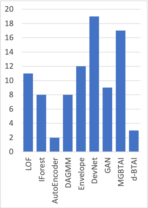
(a) Precision

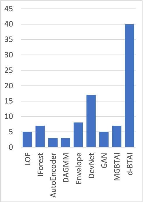
(b) Recall

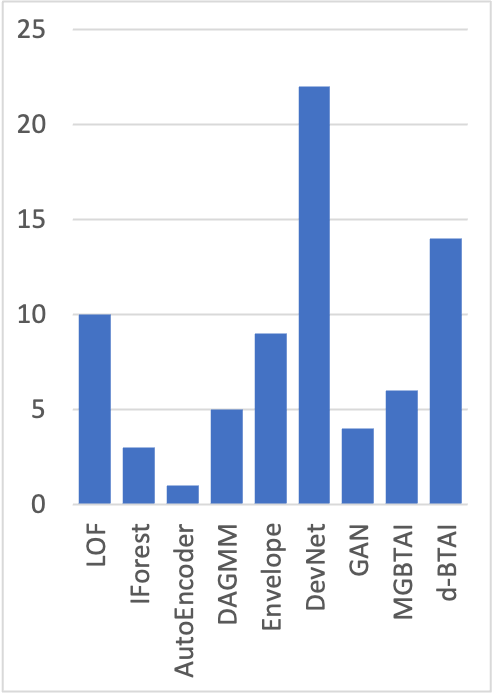
(c) F1 Score

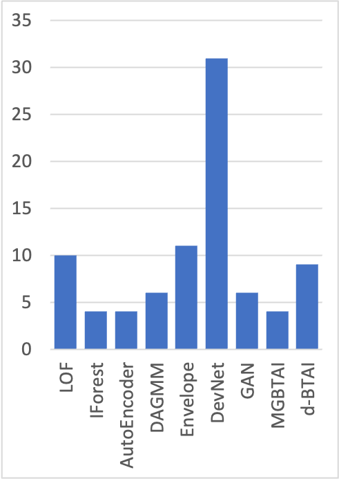
(d) AUC-ROC

Figure 2: Comparison of Algorithms using various metrics on Multivariate Datasets

Figure  2 compares algorithms based on the number of multivariate datasets in which they achieve the highest Precision, Recall, F1 score, and AUC-ROC, with each bar graph corresponding to a specific metric. In case two or more algorithms achieve the highest value for a metric on a dataset, credit is assigned to each algorithm involved.

Figure  2(a) depicts that algorithms DevNet and MGBTAI have achieved the highest precision on a majority of multivariate datasets, whereas Autoencoders obtained the maximum precision on least number of datasets. Tree-based methods exhibited outstanding performance by attaining the highest precision values across a total of 20 multivariate datasets with a perfect precision in 2 datasets. Across diverse multivariate datasets spanning various domains, tree-based methods demonstrated remarkable precision.

Figure  2(b) depicts that tree-based algorithms have achieved the highest recall on most multivariate datasets, whereas other algorithms performed very poorly. Tree-based methods excelled, achieving the highest recall in 40 datasets, securing perfect recall in 12 datasets.

Figure  2(c) depicts that the DevNet has achieved the highest F1 score overall as compared to other algorithms in 22 datasets. Tree-based methods closely followed achieving the highest F1-Score in 20 datasets.

Figure  2(d) depicts that DevNet has achieved the best AUC-ROC score overall in 31 datasets. Elliptic Envelope and LOF also performed well, achieving highest AUC-ROC in 11 and 10 datasets respectively. Tree-based Methods emerged as top performers in 13 datasets.

3.3.1 Analysis of GAN

A crucial aspect of GANs’ performance lies in its instability, as revealed through a comparative analysis of standard deviation values. The consistently high standard deviation[0-0.5774] (refer to Table 7 of the Appendix D.1) on multiple runs highlights the algorithm’s susceptibility to fluctuations, raising concerns about its stability and robustness in practical applications. This instability is further emphasized by comparing GAN with Autoencoders which prove to be a more stable alternative. The standard deviation obtained from running GAN 3 times on all datasets went as high as 0.5774 whereas that obtained from running Autoencoders had a maximum value of 0.1985.

Furthermore, GAN achieved the highest recall across 15 datasets, with a perfect recall in 14 of them. However, a closer examination revealed an interesting nuance: for 13 datasets, GAN classified all datapoints as anomalies. This peculiar outcome stemmed from the uniform discriminator score [1] assigned to all datapoints by the algorithm in the prediction of anomalies, emphasizing the need for a nuanced understanding of the algorithm’s output.

One important observation is that GAN classified all datapoints as anomalies for all 6 SWaT datasets used in this study. This raises a need to find a better algorithm for anomaly detection in SWaT datasets. SWaT datasets are multivariate time-series datasets. [13] proposed a method based on GNN to detect anomalies in multivariate time-series datasets. In our study, we have 7 multivariate time-series datasets, namely BATADAL_04, SWaT 1 to SWaT 6. When GAN is excluded from comparison, tree-based approaches and GNN are the top performers in terms of recall on these time-series datasets. Tree-based approaches obtain the highest recall on 4 datasets while GNN on 3 datasets. Furthermore, we artificially generated 6 multivariate time series datasets to continue our comparison between GNN and tree-based approaches(refer to Table 8 of the Appendix D.1). From these 6 datasets, tree-based approaches achieved the highest recall in 4 datasets. Overall, tree-based methods excelled in 8 out of 13 multivariate time-series datasets.

3.3.2 Challenges Posed by High Anomaly Prevalence in Multivariate Datasets

Anomaly detection traditionally assumes a small proportion of anomalies, typically between 2$\%$ and 10$\%$ of the dataset. However, as datasets with higher percentages of outliers, exceeding the 10$\%$ threshold, become more prevalent, the question arises whether it remains suitable to address these challenges solely through anomaly detection. Such situations often warrant a shift towards a classification approach.

Among the 73 multivariate datasets used in this benchmark, 17 have more than 10$\%$ anomalies. This makes it more suitable to treat them as a classification problem rather than an anomaly detection problem. To demonstrate this, we trained and tested a Linear Support Vector Machine (SVM) on these 17 datasets. Table 9 of the Appendix D.2 gives a thorough evaluation of the Linear SVM encompassing precision, recall, F1 Score and AUC-ROC metrics. Table 10 of the Appendix D.2 shows that linear SVM performed better and achieved the highest recall compared to all other anomaly detection algorithms in 7 of these datasets. These results strongly support the assertion that these datasets are better suited for classification rather than anomaly detection.

This research takes a deliberate step towards investigating the performance of established anomaly detection methods, notably d-BTAI and MGBTAI on datasets featuring a significantly higher anomaly prevalence, ranging from 10$\%$ to 40$\%$. While these methods were originally designed to excel in scenarios with few anomalies, our research objective is to delve into their effectiveness with datasets having a high anomaly percentage. Extending the boundaries of traditional anomaly detection scenarios we aim to highlight the adaptability of these methods in real-world settings where higher anomaly rates are encountered, acknowledging that certain domains may defy traditional assumptions which consider anomalies to be less than 10$\%$ of the dataset.

3.3.3 Analysis of OCSVM

OCSVM has proven to be a popular choice for anomaly detection due to its ability to model normal data and identify deviations effectively. However, an inherent challenge arises when the algorithm exhibits a high recall rate coupled with a low precision rate. High recall implies that the OCSVM is adept at capturing a significant portion of actual anomalies within the dataset. However, the drawback of this effectiveness lies in the concurrent low precision, indicating that a substantial number of normal instances are incorrectly classified as anomalies as seen in Table 11 and Table 12 of the Appendix D.3. The imbalance between recall and precision suggests that OCSVM tends to be overly sensitive, marking a large proportion of instances as anomalies. While this sensitivity ensures that genuine anomalies are seldom overlooked, it compromises the precision of the model by introducing a considerable number of false positives.

3.4 Results - Univariate datasets

Apart from the multivariate datasets, we have included 31 univariate datasets in our study and have tested 13 anomaly detection algorithms on these datasets. We have included 4 quantile based algorithms for the univariate study. 3 of these 4 algorithms are q-LSTM [43] with sigmoid, tanh and PEF activation functions whereas the fourth quantile based algorithm is deep quantile regression [49]. The performance of 13 anomaly detection algorithms on 31 univariate datasets is displayed in Table 14, Table 15, Table 16 and Table 17 of the Appendix D.4.

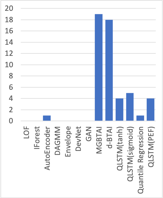
(a) Precision

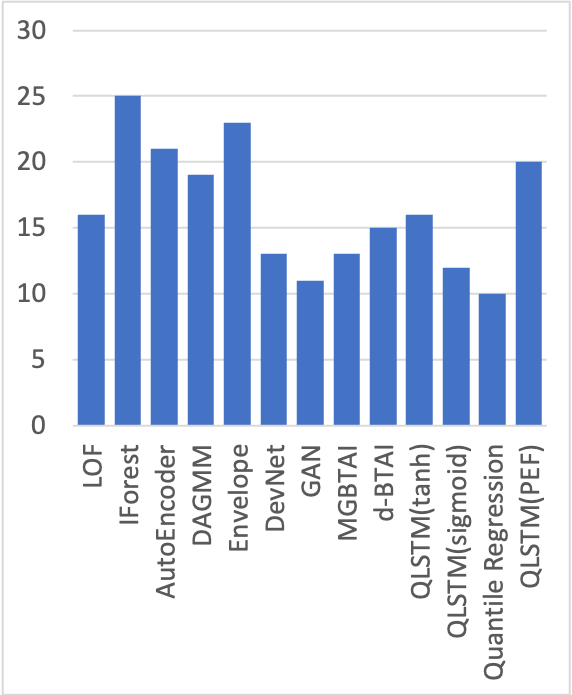
(b) Recall

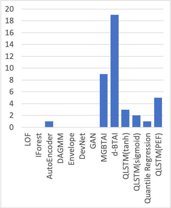
(c) F1 Score

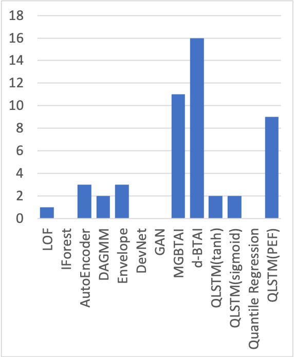
(d) AUC-ROC

Figure 3: Comparison of Algorithms using various metrics on Univariate Datasets

Figure  3 compares algorithms based on the number of univariate datasets in which they achieve the highest Precision, Recall, F1 score, and AUC-ROC. It shows that tree-based algorithms, d-BTAI and MGBTAI, emerge as dominant, excelling across all evaluation metrics. Together they achieve the highest precision in 28 out of 31 datasets as seen in figure  3(a), securing a perfect Precision in 18 datasets. q-LSTM with the sigmoid activation function stands out among the quantile based methods.

Recall is a critical metric in anomaly detection.  3(b) shows that the tree-based algorithms achieved the highest recall in 19 datasets. They also achieved a perfect recall in 18 datasets. iForest was the best performer obtaining the highest recall in 25 datasets. It was closely followed by Envelope and Autoencoder which obtained the highest recall in 23 and 21 datasets respectively. However, it’s crucial to note that these algorithms exhibit low precision as compared to tree-based algorithms which is shown in figure  3(a). Among the quantile based algorithms, q-LSTM with the PEF activation function stands out with the highest recall in 20 datasets.

In 25 out of 31 datasets, tree-based algorithms secured the highest F1 Score achieving a perfect F1 Score (1.0) in 10 datasets. As illustrated in Figure  3(c), d-BTAI consistently outperforms other algorithms in terms of F1 score, followed by MGBTAI. Among quantile based algorithms, q-LSTM with the PEF activation function stands out.

3(d) shows that tree-based algorithms achieved the highest AUC-ROC values in 20 datasets. They also obtained a perfect AUC-ROC score in 18 datasets. q-LSTM with PEF activation function also performed well and obtained the highest AUC-ROC score in 9 datasets.

In conclusion, the performance comparison of anomaly detection algorithms on univariate datasets highlights the dominance of d-BTAI and MGBTAI. Their consistent performance in precision, recall, F1 score, and AUC-ROC metrics signifies their potential to excel in various real-world applications. It is also important to note that although all the algorithms achieved high recall rates, only the tree based methods were able to couple it with a high precision.

3.5 Comparing Quantile Techniques

Table 18 of the Appendix D.5 presents an evaluation of Deep Quantile Regression and Quantile LSTM with PEF, tanh, and sigmoid activation functions across 31 univariate datasets. Quantile LSTM with PEF emerged as the top performer for 15 datasets. Quantile LSTM with tanh and sigmoid activation functions outperformed other algorithms on 5 datasets each whereas Deep Quantile Regression excelled on only 3 datasets.

3.6 Experimentation with Parameterised Elliot Function (PEF)

The Parametric Elliot Function (PEF) is a modification of the conventional activation function used in LSTM models. It has a slower saturation rate compared to other activation functions like sigmoid and tanh, which helps in overcoming the saturation problem during training and prediction. We integrated the PEF activation function into LSTM, Deep Quantile Regression, GAN , and Autoencoders, comparing their performance with models using standard tanh and sigmoid activation functions across 31 univariate datasets. This comparison has been made with respect to recall, in case of a tie between the algorithms precision is taken into consideration and in case of further tie AUC-ROC values are considered.

3.6.1 LSTM

LSTM with standard tanh and sigmoid activations performed better in 11 datasets, while those with PEF excelled in 10 datasets as seen in Table 19 of the Appendix D.6. Similar results were observed for the remaining 10 datasets.

3.6.2 Deep Quantile Regression

As shown in Table 20 of the Appendix D.6, Deep Quantile Regression using standard activation functions excelled in 17 datasets whereas Deep Quantile Regression with PEF performed well on 14 datasets.

3.6.3 GAN

While GAN with standard activation functions excelled in 9 datasets, those with PEF performed well on 3 datasets as seen in Table 21 of the Appendix D.6. Identical results were obtained for 19 datasets between GAN with PEF and GAN with standard activation functions.

3.6.4 Autoencoders

The evaluation of Autoencoders, revealed identical results for models employing standard activation functions and those utilizing PEF activation. Using PEF did not alter the performance of Autoencoders based on the considered metrics.

4 Conclusion

In this research paper, we undertook the crucial task of benchmarking anomaly detection algorithms to address the pressing need for robust anomaly detection in complex mission-critical systems. The identification of anomalies is pivotal for ensuring the resilience of such systems, and our study specifically tackled the challenge of imbalanced class distribution in operational data, where anomalies are infrequent yet critical events.

Our primary contribution lies in a comprehensive benchmark study that rigorously evaluated a diverse set of anomaly detection algorithms. Covering 104 datasets from both public and proprietary industrial systems, the research provided an unbiased comparison across classical machine learning, deep learning, and outlier detection methods. Our results demonstrate the superiority of tree-based algorithms, exemplified by MGBTAI and d-BTAI, for univariate and multivariate datasets. In particular, they stand out in identifying anomalies when there is just one in the entire set. On the other hand deep learning algorithms such as DevNet needed at least 2 anomalies to be effective. The other state of the art algorithms demonstrated high recall but suffered from notably low precision for some of the datasets. OCSVM and GAN marked most of the datapoints as anomalies. Furthermore, GAN exhibited instability, as reflected in computed standard deviations, while MGBTAI and d-BTAI demonstrated exceptional generalization ability, effectively addressing anomalies across varying volumes.

Although we have not performed any explicit comparison of false positives in this study, our experiments establish that tree-based methods outperform other algorithms in terms of precision implying that they generate less number of false positives while delivering competitive recall values. This observation is noteworthy. A report by Gartner [6] finds that automated anomaly detection technology has not been put into practice due to an unacceptably high rate of false positives in operational fault detection. Since tree based methods have impressive precision values, competitive recall, and are resilient to the diversity of anomalous instances, we believe that tree based anomaly detection methods are one of the best candidates for automated anomaly detection. If the definition of anomaly is strictly tied to the rarity of instances i.e. we define anomalous instances that are less than $10\%$ of the total instances, then tree based methods demonstrably trump all other SOTA baselines. When the anomalies are less than $10\%$, tree based methods outperform all other baselines in 45 out of 87 benchmark datasets.

Looking ahead, this benchmark study lays a robust groundwork for future advancements in the realm of anomaly detection for robust anomaly detection in complex mission-critical systems. Further exploration of hybrid models, leveraging the strengths of various algorithms, could enhance adaptability to evolving challenges in complex systems. Additionally, the study opens avenues for investigating the generalization capabilities of algorithms in dynamic environments.

Appendix A Methodology

The benchmark study comprises 104 datasets, 73 multivariate and 31 univariate datasets, detailed in section 3 of the main text. These datasets, represent diverse domains, enabling a comprehensive evaluation of anomaly detection algorithms. Dataset characterization is presented in Table2 for multivariate datasets and Table 13 for univariate datasets.

For multivariate data analysis, we employed a diverse set of anomaly detection algorithms. These include Isolation Forest (Iforest), Elliptic Envelope, Local Outlier Factor (LOF), and tree-based approaches such as MGBTAI and d-BTAI. In addition, deep learning algorithms, including Autoencoders, Dagmm, Devnet, and Generative Adversarial Networks (GAN), were utilized. We also implemented Graph Neural Networks(GNN) on 13 time series datasets. The inclusion of both traditional and deep learning-based methods ensures a comprehensive assessment .

Alongside the previously mentioned algorithms , we included quantile-based approaches, Deep Quantile Regression and q-LSTM with activation functions PEF, tanh, and sigmoid.

We further experimented with the PEF activation function and tested it on LSTM, GAN, Deep Quantile Regression and Autoencoders as discussed in section 3.6 of the main text.

The performance evaluation of anomaly detection algorithms is based on key metrics precision, recall, F1 score, and AUC ROC. The implementation details of the algorithms are comprehensively discussed in section 3.1 of the main text.

A.1 Parameter Settings for Benchmark Algorithms

In this study, we made use of established implementations wherever possible. For Isolation Forest, a contamination value of 0.12 was utilized, while other parameters adhered to default values from the sklearn package in Python. Elliptic Envelope and One-Class SVM also utilized default parameters from the sklearn package. Local Outlier Factor (LOF) was implemented using the PyOD library with its default parameters. DevNet was implemented using Deep Learning based Outlier Detection (DeepOD) library. LSTM, GAN, and Autoencoders were implemented using Keras. For autoencoders the lower threshold was set at the 0.75th percentile, and the upper threshold at the 99.25th percentile of the Mean Squared Error(MSE) values. For GAN, all the datapoints whose discriminator score lied in the lowest 10th percentile, were considered anomalies. For DAGMM, a high threshold was set as two standard deviations above the mean, and a low threshold as two standard deviations below the mean. MGBTAI, d-BTAI, GNN, q-LSTM, and deep quantile regression were implemented referring to the respective authors’ papers. For MGBTAI, minimum clustering threshold was set to 20% of the of the dataset size and leaf level threshold was set to 4, while for d-BTAI minimum clustering threshold was set to 10% of the dataset size. Both these algorithms used the k-means clustering function. For deep quantile regression the lower threshold was set at the 0.9th percentile, and the upper threshold 99.1st percentile of the predicted values. Isolation Forest, Local Outlier Factor (LOF), and Elliptic Envelope, were trained on 70% of data and tested on the entire dataset. Autoencoders, OCSVM, DAGMM, and GAN trained on 70% normal data, in cases where 70% normal data was not available, the algorithms were trained on whatever normal data was present. DevNet required 2% of the training data to be anomalous. MGBTAI and d-BTAI did not need any training data, they were directly tested on the entire dataset.

Appendix B Experimental Setting for d-BTAI

While Enhanced Cluster Based Local Outlier Factor (ECBLOF) scores are computed for all data points, it’s essential to establish a clear demarcation between normal data and anomalies. This threshold setting is manually done and is often cumbersome. Hence, we have enhanced d-BTAI for multivariate data to automatically detect the optimal threshold without manual intervention using the knee-elbow method[1].

1. Computation of ECBLOF Scores:

   The experimentation begins with the computation of anomaly scores using the ECBLOF algorithm, applied to each data point within the multivariate dataset.

2. Cumulative Sum and Percentage Conversion:

   To impart differential weightage to individual data points based on their anomaly scores, a cumulative sum is calculated which are subsequently normalized into percentage sums by dividing each cumulative sum by the largest cumulative sum.

3. Knee-Elbow Method:

   In the knee/elbow method, the idea is to find a point on the graph where the rate of change significantly slows down, often resembling the bend in a human elbow or knee. This point is considered a potential threshold. The ECBLOF scores are sorted in ascending order and the resulting plot represents indices on the x-axis and percentage sums on the y-axis, derived from the normalized cumulative sums.

4. Knee-Elbow Point Identification:

   The knee-elbow point on the plot is a distinctive point marking a significant change in the slope and is used in determining a threshold that effectively distinguishes normal behavior from anomalies within the dataset.

To understand this further let’s consider the following:

1. ECBLOF Scores:
   ECBLOF scores for three data points to be 1,2,3 and 10

2. Cumulative Sum and Percentage Conversion:

   Cumulative sums are calculated: 1, 3 (1+ 2), 6 (1 + 2 + 3), 16 (1 + 2 + 3 + 10).

   Percentage sums (normalized): 6.25% (1/16 * 100), 18.75% (3/16 * 100), 37.5% (6/16 * 100), 100% (16/16 * 100).

3. Knee-Elbow Method:

   Plotting these percentage sums on a graph with points (1, 6.25), (2, 18.75), (3, 37.5), (4, 100). The graph 4 shows a significant turn at point (3, 37.5), indicating a potential knee/elbow point.

4. Threshold Setting:

   The x-axis represents indices, and the knee/elbow method returns the index 3 which corresponds to the datapoint 10, implying that any score above 10 is marked as an anomaly.

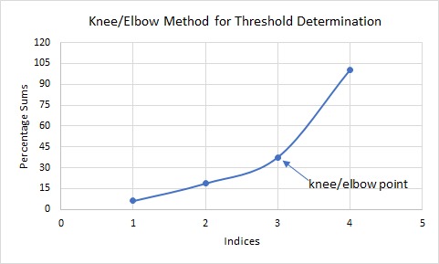
Figure 4: Visualising the elbow point

Appendix C Tree Based Methods

Among all the state of the art algorithms used in this benchmark study we would like to delve into the discussion of tree based approaches MGBTAI and d-BTAI as they have outperformed other algorithms in this benchmark study.

1. Firstly, tree based approaches are unsupervised and hence do not require training data. This is particularly useful, as training data may not always be available and if available, it may be scarce.

2. Tree based approaches are adaptable, and can be used on both temporal as well as non temporal data. They are flexible and not limited to a specific domain. They can be applied acroos various domains from finance to cybersecurity to healthcare.

3. These methods have been successful in detecting anomalies of varying densities,from detecting a singleton to thousand of anomalies as seen in the multivariate data. Unlike deep learning algorithms that have results that deviate on multiple runs, tree based approaches produce same results on all runs thus ensuring reliability.

4. Instead of creating an ensemble of binary trees like Iforest, d-BTAI employes a single binary tree making it much more efficient in terms of memory and time required for termination.

5. These approaches not only manage to accurately identify anomalies but also reduce the number of false positives and this is clearly depicted under the evaluation of univariate data as most algorithms mange to achieve a perfect recall in many datasets with tree based approaches, but when we go a step ahead and compare precision, tree based methods achieve high precision thereby emerging as clear winners.

Appendix D Results

Table 3 presents the precision values for the 9 anomaly detection algorithms across 67 multivariate datasets. MGBTAI algorithm demonstrated exceptional performance, achieving perfect precision in 2 datasets and emerging as the top performer across 17 multivariate datasets.Additionally, d-BTAI attained the highest precision in 3 datasets.Other algorithms(LOF, Iforest, Autoencoders, DAGMM, Envelope, DevNet, GAN) also achieved perfect precision in a few datasets.

Table 4 presents the recall values for the 9 anomaly detection algorithms across 67 multivariate datasets. d-BTAI stands out with perfect recall in 13 datasets and emerges as the top performer overall in 40 multivariate datasets. MGBTAI follows closely with perfect recall in 6 datasets.GAN achieved the highest recall in 15 datasets,however for 13 of these datasets it has marked all points as anomalies.

Table 5 offers a comprehensive analysis of F1-score values for nine anomaly detection algorithms applied across 67 multivariate datasets. DEVNET showcased exceptional performance, securing the highest F1 score in 22 datasets. In close pursuit, d-BTAI achieved the highest F1 score in 14 datasets, while MGBTAI in 6 datasets. Furthermore, the other algorithms, LOF, Iforest, Autoencoders, DAGMM, Envelope, and GAN, collectively demonstrated robust performance by attaining the highest F1 score in a combined total of 26 datasets.

Table 6 provides a comprehensive summary of AUC-ROC values for 9 anomaly detection algorithms applied across 67 multivariate datasets. DEVNET exhibited exceptional performance, securing the highest AUC-ROC in 30 datasets followed by d-BTAI that achieved the highest AUC-ROC in 9 datasets, while MGBTAI led in 4 datasets. Additionally, the remaining algorithms, including LOF, Iforest, Autoencoders, DAGMM, Envelope, and GAN, collectively attained the highest AUC-ROC in a combined total of 24 datasets.
The analysis of multivariate results has been discussed in detail in section 3.3 of the main text.

DATASET	SIZE	DIMENSION	# ANOMALIES	% ANOMALIES	Domain
ALOI	49534	27	1508	3.04	Image
annthyroid	7200	6	534	7.42	Healthcare
backdoor	95329	196	2329	2.44	Network
breastw	683	9	239	34.99	Healthcare
campaign	41188	62	4640	11.27	Finance
cardio	1831	21	176	9.61	Healthcare
Cardiotocography	2114	21	466	22.04	Healthcare
celeba	202599	39	4547	2.24	Image
cover	286048	10	2747	0.96	Botany
donors	619326	10	36710	5.93	Sociology
fault	1941	27	673	34.67	Physical
fraud	284807	29	492	0.17	Finance
glass	214	7	9	4.21	Forensic
Hepatitis	80	19	13	16.25	Healthcare
http	567498	3	2211	0.39	Web
InternetAds	1966	1555	368	18.72	Image
Ionosphere	351	33	126	35.9	Mineralogy
landsat	6435	36	1333	20.71	Astronautics
letter	1600	32	100	6.25	Image
Lymphography	148	18	6	4.05	Healthcare
magic.gamma	19020	6	260	1.37	Physical
mammography	11183	6	260	2.32	Healthcare
mnist	7603	100	700	9.21	Image
musk	3062	166	97	3.17	Chemistry
optdigits	5216	64	150	2.88	Image
PageBlocks	5393	10	510	9.46	Document
pendigits	6870	16	156	2.27	Image
Pima	768	8	268	34.9	Healthcare
satellite	6435	36	2036	31.64	Astronautics
satimage-2	5803	36	71	1.22	Astronautics
shuttle	49097	9	3511	7.15	Astronautics
skin	245057	3	50859	20.75	Image
smtp	95156	3	30	0.03	Web
SpamBase	4207	57	1679	39.91	Document
speech	3686	400	61	1.65	Linguistics
Stamps	340	9	31	9.12	Document
thyroid	3772	6	93	2.47	Healthcare
vertebral	240	6	30	12.5	Biology
vowels	1456	12	50	3.43	Linguistics
Waveform	3443	21	100	2.9	Physics
WBC	223	9	10	4.48	Healthcare
WDBC	367	30	10	2.72	Healthcare
Wilt	4819	5	257	5.33	Botany
wine	129	13	10	7.75	Chemistry
WPBC	198	33	47	23.74	Healthcare
yeast	1484	8	507	34.16	Biology
CIFAR10	5263	512	263	5	Image
FashionMNIST	6315	512	315	5	Image
MNIST-C	10000	512	500	5	Image
MVTec-AD	292	512	63	21.5	Image
SVHN	5208	512	260	5	Image
Agnews	10000	768	500	5	NLP
Amazon	10000	768	500	5	NLP
Imdb	10000	768	500	5	NLP
Yelp	10000	768	500	5	NLP
20newsgroups	3090	768	155	5	NLP
BATADAL$\_$04	4177	43	219	5.24	Industrial
SWaT 1	50400	51	4466	8.86	Industrial
SWaT 2	86400	51	4216	4.88	Industrial
SWaT 3	86400	51	3075	3.56	Industrial
SWaT 4	86319	51	37559	43.51	Industrial
SWaT 5	86400	51	2167	2.51	Industrial
SWaT 6	54000	51	3138	5.81	Industrial
ecoli	336	7	9	2.68	Healthcare
cmc	1473	9	17	1.15	Healthcare
lympho_h	148	18	6	4.05	Healthcare
wbc_h	378	30	21	5.56	Healthcare

Table 2: Multivariate Datasets Characterisation

Dataset	LOF	IForest	AutoEncoders	DAGMM	Elliptic Envelope	DevNet	GAN	MGBTAI	d-BTAI
ALOI	0.1	0.04	0.05	0.03	0.03	0.03	0.04	0.04	0.04
annthyroid	0.26	0.25	0.15	0.24	0.4	0.12	0.09	0.07	0.11
backdoor	0.11	0.03	0.2	0.21	0.21	0.21	0.21	0.01	0.06
breastw	0.39	0.98	0.27	1	1	0.86	0	0.85	0.89
campaign	0.07	0.33	0.22	0.3	0.34	0.42	0.21	0.17	0.16
cardio	0.17	0.48	0.34	0.13	0.4	0.5	0.07	0.48	0.2
Cardiotocography	0.32	0.48	0.31	0.36	0.48	0.4	0.24	0.8	0.35
celeba	0.01	0.07	0.02	0.07	0.09	0.19	0.03	0.08	0.03
cover	0.02	0.05	0.09	0.02	0.01	0.1	0.01	0	0.02
donors	0.21	0.1	0.14	0.5	0.2	0.44	0.04	0	0.13
fault	0.32	0.49	0.19	0.36	0.24	0.36	0.47	0.42	0.49
fraud	0	0.02	0.02	0.01	0.02	0.02	NA	0.01	0
glass	0.18	0.1	0.09	0	0.12	0	0.06	0.08	0.17
Hepatitis	0.25	0.18	0.13	0.25	0.33	0.25	0.2	0	0.14
http	0	0.03	0.04	0.04	0.04	0.04	NA	0.05	0.03
InternetAds	0.48	0.64	0.53	0.2	0.63	0.32	0.11	0.98	0.28
Ionosphere	0.94	0.96	0.5	0.69	1	0.58	0.58	0.44	0.82
landsat	0.31	0.15	0.19	0.18	0.04	0.24	0.38	0.01	0.26
letter	0.36	0.08	0.05	0.06	0.17	0.07	0.06	0.11	0.12
Lymphography	0.33	0.4	0.13	0.07	0.38	0.11	0.13	0.43	0.15
magic.gamma	0.62	0.78	0.55	0.56	0.91	0.78	0.76	0.77	0.53
mammography	0.08	0.12	0.05	0.15	0.03	0.19	0.01	0	0.07
mnist	0.23	0.32	0.19	0.16	0.16	0.47	0.09	0.02	0.17
musk	0.01	0.25	0.17	0.32	0.31	0.29	0.03	0.23	0.36
optdigits	0.07	0.05	0.04	0.05	0	0.26	0.03	0.33	0.02
PageBlocks	0.39	0.41	0.29	0.27	0.56	0.17	0.31	0.67	0.17
pendigits	0.04	0.16	0.13	0	0.06	0.23	0.06	0	0.04
Pima	0.32	0.59	0.35	0.45	0.51	0.68	0.15	0.28	0.44
satellite	0.48	0.93	0.39	0.77	0.96	0.59	0.32	1	0.54
satimage-2	0.03	0.1	0	0.08	0.12	0.12	0.01	0.14	0.04
shuttle	0	0.98	0.47	0.51	1	0.48	0.07	0.49	0.44
skin	0.24	0.06	0.08	0.57	0.3	0.76	0.1	0.62	0.27
smtp	0.002	0.002	0.002	0.003	0.002	0.002	0.003	0.003	0.001
SpamBase	0.32	0.41	0.41	0.63	0.31	0.76	0.08	0.73	0.66
speech	0.02	0.02	0.03	0.01	0.02	0.13	0.08	0.01	0.02
Stamps	0.15	0.23	0.14	0.03	0.11	0.15	0.45	0.13	0.15
thyroid	0.1	0.19	0.15	0.17	0.23	0.18	0.17	0.13	0.08
vertebral	0.04	0.03	0	0.08	0	0.1	0.04	0	0.05
vowels	0.26	0.09	0.11	0.01	0.05	0.19	0.03	0.67	0.08
Waveform	0.09	0.06	0.11	0.09	0.04	0.07	0.21	0	0.05
WBC	0.09	0.32	0.38	0.35	0.38	0.31	0.06	0.42	0.19
WDBC	0.27	0.21	0.26	0.24	0.26	0.26	0.01	0.21	0.19
Wilt	0.1	0.01	0.05	0.1	0.1	0	0.05	0	0.05
wine	0.77	0.18	0.5	0.31	0.36	0.45	0.51	0.53	0.26
WPBC	0.1	0.14	0.25	0.15	0.15	0.18	0.2	0.12	0.25
yeast	0.27	0.3	0.35	0.36	0.26	0.35	0.49	0.1	0.3
CIFAR10	0.14	0.13	0.07	0.05	0.13	0.17	0.18	0.04	0.08
FashionMNIST	0.15	0.19	0.12	0.11	0.18	0.29	0.21	0.06	0.1
MNIST-C	0.13	0.08	0.04	0.08	0.08	0.38	0.09	0.05	0.17
MVTec-AD	0.87	1	0.5	0.4	0.12	0.26	0.97	1	0.9
SVHN	0.11	0.06	0.04	0.05	0.09	0.38	0.1	0.06	0.1
Agnews	0.11	0.06	0.05	0.06	0.07	0.07	0.1	0.05	0.06
Amazon	0.06	0.06	0.05	0.05	0.06	0.06	0.06	0.05	0.05
Imdb	0.04	0.04	0.05	0.05	0.03	0.07	0	0.02	0.05
Yelp	0.1	0.09	0.03	0.06	0.07	0.06	0.04	0.04	0.06
20newsgroups	0.18	0.07	0.05	0.06	0.1	0.05	0.04	0	0.04
BATADAL$\_$04	0.2	0.1	0.09	0.19	0.26	0.05	0.1	0.1	0.09
SWaT 1	0.08	0.63	0.13	0.5	0.19	0.22	0.09	0.63	0.19
SWaT 2	0.06	0.71	0.1	0.11	0.13	0.12	0.05	0.71	0.08
SWaT 3	0.04	0.02	0.13	0.23	0.09	0.15	0.04	0.02	0.07
SWaT 4	0.45	0.34	0.08	0.99	0.27	0.88	0.44	0.34	0.18
SWaT 5	0.02	0.22	0.09	0.1	0.12	0.12	0.03	0.22	0.06
SWaT 6	0.07	0.97	0.37	0.26	0.26	0.17	0.06	0.97	0.13
ecoli	0.21	0.19	0.2	0.22	0.21	0.06	0	0.14	0.06
cmc	0.01	0	0.03	0.01	0.01	0	0.05	0	0.02
lympho h	0.33	0.32	0.12	0	0.21	0.06	0.05	0	0.11
wbc h	0.37	0.34	0.27	0.32	0.35	0.4	0.04	0.61	0.17

Table 3: Precision values of the 9 algorithms on the 67 multivariate datasets. The highest value(s) is marked in bold. The notation (NA) denotes that the algorithm exceeded a runtime of three hours without successfully generating results.

Dataset	LOF	Iforest	AutoEncoders	DAGMM	Elliptic Envelope	DevNet	GAN	MGBTAI	d-BTAI
ALOI	0.34	0.15	0.12	0.11	0.09	0.08	0.14	0.13	0.4
annthyroid	0.35	0.41	0.2	0.32	0.52	0.17	0.12	0.18	0.51
backdoor	0.45	0.16	0.19	0.87	0.84	0.91	0.86	0.02	0.87
breastw	1	0.41	0.13	0.29	0.32	1	0	0.33	0.87
campaign	0.06	0.35	0.19	0.27	0.31	0.52	0.19	0.16	0.66
cardio	0.18	0.61	0.36	0.14	0.42	0.79	0.07	0.32	0.76
Cardiotocography	0.15	0.26	0.13	0.16	0.21	0.23	0.32	0.2	0.47
celeba	0.05	0.38	0.1	0.29	0.38	0.88	0.15	0.7	0.38
cover	0.22	0.57	0.37	0.24	0.13	0.97	1	0	0.7
donors	0.33	0.2	0.24	0.86	0.33	1	0.1	0	0.47
fault	0.09	0.18	0.24	0.1	0.07	0.11	0.14	0.07	0.6
fraud	0.11	0.89	0.88	0.62	0.85	0.92	NA	0.62	0.96
glass	0.44	0.33	0.22	0	0.33	0	0.13	0.11	1
Hepatitis	0.15	0.15	0.08	0.15	0.31	0.15	0.12	0	0.23
http	0.03	1	1	1	1	1	NA	1	1
InternetAds	0.26	0.42	0.29	0.11	0.36	0.17	0.04	0.23	0.6
Ionosphere	0.26	0.35	0.14	0.2	0.25	0.25	0.16	0.03	0.84
landsat	0.15	0.09	0.09	0.09	0.02	0.12	0.19	0	0.46
letter	0.57	0.16	0.08	0.09	0.28	0.12	0.1	0.18	0.86
Lymphography	0.83	1	0.33	0.17	0.83	0.33	0.33	1	1
magic.gamma	0.18	0.26	0.16	0.16	0.26	0.57	0.22	0.21	0.59
mammography	0.37	0.64	0.42	0.64	0.13	0.8	0.04	0	0.84
mnist	0.25	0.42	0.21	0.18	0.18	0.71	1	0.02	0.85
musk	0.04	1	0.53	1	1	1	1	0.79	1
optdigits	0.26	0.21	0.15	0.16	0.01	0.99	0.12	0.81	0.27
PageBlocks	0.41	0.52	0.3	0.29	0.61	0.2	0.33	0.06	0.21
pendigits	0.17	0.88	0.56	0.01	0.28	0.98	0.25	0.03	0.72
Pima	0.09	0.23	0.1	0.13	0.16	0.36	0.04	0.05	0.43
satellite	0.15	0.34	0.12	0.24	0.29	0.31	1	0.3	0.59
satimage-2	0.28	0.99	0.01	0.65	1	0.97	1	1	1
shuttle	0	0.41	0.65	0.72	0.31	0.98	1	0.01	0.88
skin	0.12	0.03	0.04	0.28	0.14	1	0.05	0.15	0.22
smtp	0.7	0.77	0.7	0.87	0.77	0.7	1	0.33	0.87
SpamBase	0.08	0.12	0.1	0.16	0.07	0.45	0.02	0.18	0.26
speech	0.15	0.15	0.18	0.03	0.11	0.75	0.12	0.11	0.8
Stamps	0.16	0.32	0.15	0.03	0.13	0.16	0.49	0.06	0.61
thyroid	0.39	0.97	0.62	0.71	0.96	0.72	0.71	0.25	1
vertebral	0.03	0.03	0	0.07	0	0.07	0.03	0	0.13
vowels	0.76	0.3	0.33	0.02	0.14	0.62	0.08	0.16	1
Waveform	0.31	0.25	0.37	0.32	0.16	0.24	0.72	0	0.76
WBC	0.2	1	0.9	0.8	1	1	0.13	1	1
WDBC	1	1	1	0.9	0.9	1	0.33	1	1
Wilt	0.19	0.02	0.1	0.18	0.2	0	1	0	0.18
wine	1	0.3	0.7	0.4	0.4	1	0.67	1	1
WPBC	0.04	0.09	0.11	0.06	0.06	0.06	0.09	0.04	0.4
yeast	0.08	0.1	0.1	0.11	0.08	0.1	0.14	0	0.27
CIFAR10	0.27	0.31	0.14	0.1	0.26	0.37	0.37	0.07	0.71
FashionMNIST	0.3	0.47	0.24	0.22	0.36	0.71	0.42	0.12	0.93
MNIST-C	0.27	0.18	0.08	0.15	0.15	0.97	0.18	0.12	0.85
MVTec-AD	0.41	0.51	0.24	0.19	0.21	0.13	0.46	0.22	0.87
SVHN	0.22	0.13	0.08	0.1	0.2	0.96	0.2	0.06	0.88
Agnews	0.22	0.15	0.09	0.12	0.14	0.14	0.21	0.02	0.47
Amazon	0.12	0.14	0.1	0.11	0.12	0.12	0.11	0.12	0.47
Imdb	0.08	0.08	0.1	0.1	0.06	0.13	0	0.02	0.43
Yelp	0.2	0.21	0.07	0.11	0.14	0.11	0.08	0.04	0.54
20newsgroups	0.37	0.17	0.11	0.13	0.19	0.1	0.08	0	0.29
BATADAL$\_$04	0.38	0.1	0.17	0.36	0.5	0.10	0.23	0.1	0.75
SWaT 1	0.09	0.15	0.15	0.57	0.21	0.23	1	0.15	0.81
SWaT 2	0.13	0.08	0.2	0.23	0.27	0.26	1	0.08	0.53
SWaT 3	0.12	0.03	0.38	0.65	0.24	0.42	1	0.03	0.69
SWaT 4	0.1	0.12	0.02	0.23	0.06	0.89	1	0.12	0.15
SWaT 5	0.08	0.22	0.36	0.38	0.51	0.5	1	0.22	0.83
SWaT 6	0.12	0.4	0.63	0.44	0.44	0.30	1	0.4	0.81
ecoli	0.78	0.78	0.78	0.78	0.78	0.22	0	0.78	0.78
cmc	0.06	0	0.24	0.06	0.12	0	0.47	0	0.47
lympho h	0.83	1	0.33	0	0.67	0.17	0.11	0	1
wbc h	0.67	0.71	0.48	0.57	0.67	1	0.08	0.52	1

Table 4: Recall values of the 9 algorithms on the 67 multivariate datasets. The highest value(s) is marked in bold.

Dataset	LOF	Iforest	AutoEncoders	DAGMM	Elliptic Envelope	DevNet	GAN	MGBTAI	d-BTAI
ALOI	0.16	0.06	0.06	0.05	0.04	0.04	0.06	0.07	0.06
annthyroid	0.3	0.31	0.17	0.28	0.45	0.14	0.1	0.1	0.19
backdoor	0.18	0.05	0.26	0.34	0.33	0.35	0.34	0.02	0.11
breastw	0.56	0.57	0.26	0.45	0.49	0.92	0	0.48	0.88
campaign	0.06	0.34	0.2	0.28	0.32	0.47	0.2	0.16	0.26
cardio	0.18	0.54	0.35	0.13	0.41	0.61	0.07	0.38	0.32
Cardiotocography	0.2	0.34	0.19	0.22	0.29	0.29	0.22	0.32	0.4
celeba	0.02	0.12	0.04	0.11	0.14	0.32	0.05	0.14	0.06
cover	0.04	0.09	0.17	0.04	0.02	0.17	0.02	0	0.04
donors	0.26	0.13	0.19	0.63	0.25	0.61	0.06	0	0.2
fault	0.15	0.26	0.38	0.16	0.11	0.16	0.21	0.12	0.54
fraud	0	0.03	0.03	0.02	0.04	0.03	NA	0.02	0.01
glass	0.26	0.16	0.13	0	0.18	0	0.08	0.09	0.29
Hepatitis	0.19	0.17	0.1	0.19	0.32	0.19	0.15	0	0.18
http	0	0.06	0.07	0.07	0.07	0.08	NA	0.08	0.06
InternetAds	0.33	0.42	0.37	0.14	0.46	0.22	0.16	0.38	0.39
Ionosphere	0.41	0.51	0.22	0.31	0.39	0.35	0.25	0.06	0.83
landsat	0.2	0.11	0.13	0.12	0.02	0.16	0.25	0	0.33
letter	0.57	0.11	0.06	0.07	0.22	0.09	0.07	0.13	0.21
Lymphography	0.48	0.57	0.18	0.1	0.53	0.17	0.19	0.6	0.26
magic.gamma	0.27	0.39	0.24	0.25	0.4	0.66	0.34	0.33	0.56
mammography	0.14	0.21	0.09	0.24	0.05	0.3	0.02	0	0.13
mnist	0.24	0.37	0.2	0.17	0.17	0.56	0.17	0.02	0.28
musk	0.02	0.39	0.25	0.48	0.47	0.45	0.06	0.35	0.53
optdigits	0.12	0.08	0.07	0.07	0	0.42	0.05	0.47	0.03
PageBlocks	0.4	0.46	0.3	0.28	0.58	0.18	0.32	0.11	0.19
pendigits	0.06	0.28	0.21	0	0.11	0.37	0.09	0	0.08
Pima	0.14	0.33	0.16	0.2	0.24	0.47	0.07	0.09	0.43
satellite	0.23	0.5	0.19	0.37	0.45	0.41	0.48	0.46	0.57
satimage-2	0.28	0.18	0	0.14	0.21	0.22	0.02	0.25	0.07
shuttle	0	0.57	0.54	0.6	0.48	0.64	0.13	0.01	0.59
skin	0.16	0.04	0.05	0.37	0.19	0.86	0.07	0.24	0.24
smtp	0.004	0.004	0.004	0.005	0.005	0.004	0.001	0.004	0.002
SpamBase	0.13	0.18	0.16	0.25	0.12	0.57	0.03	0.29	0.37
speech	0.04	0.04	0.05	0.01	0.03	0.23	0.03	0.03	0.03
Stamps	0.15	0.27	0.14	0.03	0.12	0.15	0.47	0.09	0.24
thyroid	0.15	0.32	0.24	0.28	0.37	0.29	0.28	0.17	0.14
vertebral	0.04	0.03	0	0.07	0	0.08	0.04	0	0.07
vowels	0.39	0.14	0.17	0.01	0.07	0.3	0.0408	0.26	0.14
Waveform	0.14	0.09	0.17	0.14	0.07	0.11	0.32	0	0.09
WBC	0.12	0.49	0.53	0.48	0.56	0.48	0.08	0.57	0.31
WDBC	0.43	0.35	0.42	0.38	0.4	0.41	0.02	0.34	0.32
Wilt	0.14	0.01	0.07	0.12	0.13	0	0.1	0	0.07
wine	0.87	0.22	0.58	0.35	0.38	0.55	0.58	0.69	0.42
WPBC	0.06	0.11	0.15	0.09	0.09	0.09	0.12	0.06	0.31
yeast	0.12	0.16	0.16	0.16	0.12	0.16	0.22	0.01	0.28
CIFAR10	0.18	0.18	0.09	0.07	0.18	0.23	0.25	0.05	0.14
FashionMNIST	0.2	0.27	0.16	0.15	0.24	0.41	0.28	0.08	0.18
MNIST-C	0.18	0.11	0.06	0.1	0.1	0.55	0.12	0.07	0.28
MVTec-AD	0.56	0.67	0.32	0.26	0.15	0.17	0.62	0.36	0.89
SVHN	0.15	0.08	0.06	0.06	0.13	0.55	0.12	0.06	0.18
Agnews	0.15	0.09	0.06	0.08	0.09	0.09	0.14	0.03	0.11
Amazon	0.08	0.08	0.07	0.07	0.08	0.08	0.07	0.07	0.1
Imdb	0.06	0.05	0.07	0.07	0.04	0.09	0	0.02	0.5
Yelp	0.13	0.12	0.06	0.07	0.1	0.07	0.06	0.04	0.56
20newsgroups	0.25	0.1	0.09	0.09	0.13	0.06	0.06	0	0.47
BATADAL$\_$04	0.26	0.1	0.12	0.25	0.34	0.07	0.14	0.1	0.17
SWaT 1	0.09	0.24	0.14	0.53	0.2	0.22	0.16	0.24	0.31
SWaT 2	0.08	0.15	0.13	0.15	0.18	0.16	0.04	0.15	0.14
SWaT 3	0.06	0.02	0.2	0.34	0.13	0.23	0.04	0.02	0.13
SWaT 4	0.17	0.18	0.03	0.37	0.1	0.89	0.44	0.18	0.16
SWaT 5	0.03	0.22	0.15	0.15	0.2	0.17	0.02	0.22	0.12
SWaT 6	0.09	0.57	0.46	0.33	0.32	0.20	0.06	0.57	0.22
ecoli	0.33	0.3	0.31	0.33	0.21	0.1	0	0.23	0.1
cmc	0.01	0	0.06	0.01	0.03	0	0.1	0	0.03
lympho h	0.48	0.48	0.18	0	0.32	0.09	0.07	0	0.2
wbc h	0.47	0.46	0.35	0.41	0.46	0.57	0.06	0.56	0.29

Table 5: F1 Score values of the 9 algorithms on the 67 multivariate datasets. The highest value(s) is marked in bold.

Dataset	LOF	Iforest	AutoEncoders	DAGMM	Elliptic Envelope	DevNet	GAN	MGBTAI	d-BTAI
ALOI	0.63	0.51	0.51	0.51	0.49	0.49	0.52	0.52	0.53
annthyroid	0.63	0.66	0.55	0.62	0.73	0.54	0.51	0.5	0.6
backdoor	0.68	0.52	0.53	0.89	0.88	0.91	0.89	0.49	0.76
breastw	0.57	0.7	0.63	0.64	0.66	0.95	0.41	0.65	0.91
campaign	0.48	0.63	0.55	0.59	0.62	0.72	0.55	0.53	0.61
cardio	0.55	0.77	0.64	0.52	0.68	0.85	0.4	0.64	0.72
Cardiotocography	0.53	0.59	0.55	0.54	0.57	0.67	0.5	0.59	0.61
celeba	0.47	0.63	0.5	0.6	0.64	0.9	0.52	0.75	0.55
cover	0.56	0.73	0.91	0.57	0.52	0.94	0.5	0.5	0.68
donors	0.63	0.54	0.6	0.9	0.62	0.96	0.47	0.5	0.63
fault	0.5	0.54	0.68	0.5	0.48	0.5	0.53	0.51	0.63
fraud	0.51	0.88	0.89	0.77	0.88	0.91	NA	0.75	0.78
glass	0.68	0.6	0.56	0.50	0.61	0.50	0.52	0.53	0.89
Hepatitis	0.53	0.51	0.49	0.53	0.59	0.53	0.51	0.44	0.48
http	0.47	0.94	0.95	0.95	0.95	0.95	NA	0.95	0.94
InternetAds	0.6	0.68	0.61	0.5	0.66	0.54	0.47	0.62	0.63
Ionosphere	0.63	0.67	0.53	0.57	0.62	0.57	0.55	0.5	0.87
landsat	0.53	0.48	0.5	0.49	0.45	0.51	0.55	0.44	0.56
letter	0.75	0.52	0.49	0.49	0.6	0.51	0.5	0.54	0.72
Lymphography	0.88	0.97	0.62	0.53	0.89	0.61	0.62	0.97	0.88
magic.gamma	0.56	0.61	0.54	0.55	0.62	0.74	0.59	0.59	0.65
mammography	0.64	0.77	0.58	0.78	0.52	0.86	0.47	0.5	0.8
mnist	0.58	0.67	0.56	0.54	0.54	0.82	0.5	0.46	0.71
musk	0.47	0.95	0.72	0.96	0.96	0.96	0.5	0.85	0.82
optdigits	0.58	0.55	0.52	0.53	0.45	0.96	0.51	0.88	0.42
PageBlocks	0.67	0.72	0.61	0.6	0.78	0.55	0.62	0.53	0.55
pendigits	0.53	0.89	0.74	0.46	0.59	0.95	0.58	0.41	0.67
Pima	0.49	0.57	0.5	0.52	0.54	0.64	0.46	0.49	0.57
satellite	0.54	0.66	0.52	0.6	0.64	0.61	0.5	0.65	0.68
satimage-2	0.59	0.94	0.46	0.78	0.95	0.94	0.5	0.92	0.83
shuttle	0.43	0.7	0.8	0.83	0.66	0.95	0.5	0.5	0.9
skin	0.51	0.45	0.46	0.61	0.53	0.96	0.47	0.56	0.53
smtp	0.8	0.82	0.8	0.88	0.83	0.8	0.5	0.64	0.81
SpamBase	0.48	0.5	0.5	0.55	0.48	0.68	0.43	0.57	0.58
speech	0.52	0.51	0.54	0.47	0.51	0.84	0.51	0.49	0.48
Stamps	0.53	0.61	0.53	0.46	0.51	0.53	0.72	0.51	0.63
thyroid	0.65	0.93	0.76	0.81	0.94	0.82	0.81	0.6	0.84
vertebral	0.46	0.44	0.44	0.48	0.44	0.49	0.31	0.49	0.39
vowels	0.84	0.6	0.62	0.46	0.52	0.76	0.49	0.58	0.79
Waveform	0.61	0.56	0.64	0.61	0.53	0.57	0.82	0.5	0.64
WBC	0.55	0.95	0.91	0.86	0.96	0.95	0.52	0.97	0.9
WDBC	0.96	0.95	0.96	0.91	0.91	0.96	0.46	0.95	0.94
Wilt	0.55	0.44	0.5	0.54	0.55	0.45	0.5	0.48	0.48
wine	0.99	0.59	0.82	0.66	0.67	0.95	0.81	0.96	0.88
WPBC	0.46	0.46	0.5	0.48	0.48	0.49	0.49	0.47	0.51
yeast	0.48	0.49	0.5	0.5	0.48	0.5	0.53	0.49	0.47
CIFAR10	0.59	0.6	0.52	0.5	0.59	0.68	0.64	0.49	0.64
FashionMNIST	0.6	0.68	0.58	0.56	0.64	0.81	0.67	0.51	0.76
MNIST-C	0.59	0.53	0.49	0.53	0.53	0.94	0.54	0.5	0.71
MVTec-AD	0.7	0.75	0.59	0.56	0.39	0.51	0.73	0.61	0.92
SVHN	0.56	0.51	0.49	0.5	0.55	0.94	0.58	0.51	0.73
Agnews	0.56	0.51	0.5	0.51	0.52	0.51	0.56	0.5	0.55
Amazon	0.51	0.51	0.5	0.5	0.51	0.51	0.51	0.5	0.5
Imdb	0.49	0.48	0.5	0.5	0.48	0.52	0.5	0.48	0.5
Yelp	0.55	0.55	0.48	0.51	0.52	0.51	0.49	0.5	0.56
20newsgroups	0.64	0.53	0.51	0.52	0.55	0.5	0.49	0.5	0.47
BATADAL$\_$04	0.65	0.52	0.54	0.64	0.71	0.50	0.55	0.52	0.68
SWaT 1	0.5	0.57	0.53	0.76	0.56	0.57	0.5	0.57	0.74
SWaT 2	0.51	0.54	0.55	0.57	0.59	0.58	0.5	0.54	0.61
SWaT 3	0.51	0.48	0.64	0.79	0.57	0.66	0.5	0.48	0.68
SWaT 4	0.5	0.47	0.43	0.61	0.47	0.9	0.5	0.47	0.31
SWaT 5	0.49	0.6	0.63	0.65	0.71	0.70	0.5	0.6	0.75
SWaT 6	0.51	0.7	0.78	0.68	0.68	0.60	0.5	0.7	0.74
ecoli	0.85	0.84	0.83	0.85	0.85	0.57	0.5	0.82	0.71
cmc	0.48	0.44	0.59	0.48	0.51	0.45	0.69	0.46	0.57
lympho h	0.88	0.95	0.62	0.45	0.78	0.53	0.5	0.44	0.83
wbc h	0.8	0.82	0.71	0.75	0.8	0.96	0.49	0.75	0.86

Table 6: AUC-ROC values of the 9 algorithms on the 67 multivariate datasets. The highest value(s) is marked in bold.

D.1 Analysing GAN

Generative Adversarial Networks (GAN) and Autoencoders were executed three times, and the mean as well as the standard deviation were computed for each run as displayed in Table 7. Results revealed a significant deviation in the performance of GAN compared to Autoencoders as discussed under Analysis of GAN in section 3.3.1 of the main text.

Dataset	AUTOENCODERS				GAN
	Precision($\mu\pm\sigma$)	Recall($\mu\pm\sigma$)	F1 Score($\mu\pm\sigma$)	AUC-ROC($\mu\pm\sigma$)	Precision($\mu\pm\sigma$)	Recall($\mu\pm\sigma$)	F1 Score($\mu\pm\sigma$)	AUC-ROC($\mu\pm\sigma$)
ALOI	0.05±0.0267	0.12±0.0063	0.06±0.003	0.51±0.0032	0.04±0.0006	0.14±0.0021	0.06±0.0012	0.52±0
annthyroid	0.15±0.004	0.2±0.0056	0.17±0.0045	0.55±0.0029	0.09±0	0.12±0	0.1±0	0.51±0
backdoor	0.2±0.0247	0.19±0.0443	0.26±0.0699	0.53±0.0473	0.21±0.0014	0.86±0.0056	0.34±0.0022	0.89±0.0028
breastw	0.27±0.0587	0.13±0.064	0.26±0.0623	0.63±0.083	0±0	0±0	0±0	0.41±0.0089
campaign	0.22±0.0233	0.19±0.0207	0.2±0.0219	0.55±0.0116	0.21±0.0755	0.19±0.0758	0.2±0.0758	0.55±0.0412
cardio	0.34±0.0137	0.36±0.0143	0.35±0.0142	0.64±0.0079	0.07±0.051	0.07±0.0589	0.07±0.0589	0.4±0.2081
Cardiotocography	0.31±0.0485	0.13±0.0026	0.19±0.0197	0.55±0.0577	0.24±0.0575	0.32±0.3818	0.22±0.0861	0.5±0.0207
celeba	0.02±0.0044	0.1±0.0195	0.04±0.0072	0.5±0.0101	0.03±0.028	0.15±0.125	0.05±0.0458	0.52±0.0639
cover	0.09±0.0014	0.37±0.1985	0.17±0.014	0.91±0.0173	0.01±0	1±0	0.02±0	0.5±0
donors	0.14±0.0058	0.24±0.0062	0.19±0.0373	0.6±0.0618	0.04±0.0413	0.1±0.0869	0.06±0.0546	0.47±0.0442
fault	0.19±0	0.24±0.0006	0.38±0	0.68±0	0.47±0.245	0.14±0.245	0.21±0.0283	0.53±0.0134
fraud	0.02±0.0001	0.88±0	0.03±0	0.89±0.0001	NA	NA	NA	0±NA
glass	0.09±0.0787	0.22±0.1924	0.13±0.1118	0.56±0.1005	0.06±0.0539	0.13±0.1434	0.08±0.0832	0.52±0.0737
Hepatitis	0.13±0	0.08±0	0.1±0	0.49±0	0.2±0.1	0.12±0.0671	0.15±0.085	0.51±0.0402
http	0.04±0	1±0	0.07±0.0001	0.95±0	NA	NA	NA	0±NA
InternetAds	0.53±0	0.29±0	0.37±0	0.61±0	0.11±0.0467	0.04±0.0207	0.16±0.1934	0.47±0.0187
Ionosphere	0.5±0	0.14±0	0.22±0	0.53±0	0.58±0.2589	0.16±0.0829	0.25±0.1286	0.55±0.0644
landsat	0.19±0.0614	0.09±0.0296	0.13±0.04	0.5±0.0187	0.38±0.0376	0.19±0.0195	0.25±0.0259	0.55±0.0114
letter	0.05±0	0.08±0	0.06±0	0.49±0	0.06±0.0172	0.1±0.0321	0.07±0.0241	0.5±0.0192
Lymphography	0.13±0	0.33±0	0.18±0	0.62±0	0.13±0.1254	0.33±0.3524	0.19±0.2039	0.62±0.1827
magic.gamma	0.55±0.013	0.16±0.0037	0.24±0.0058	0.54±0.0029	0.76±0.1388	0.22±0.0432	0.34±0.0671	0.59±0.0339
mammography	0.05±0.0381	0.42±0.0077	0.09±0.0578	0.58±0.068	0.01±0.004	0.04±0.0182	0.02±0.0055	0.47±0.0071
mnist	0.19±0.0013	0.21±0.0015	0.2±0.0014	0.56±0.0008	0.09±0	1±0	0.17±0	0.5±0
musk	0.17±0	0.53±0	0.25±0	0.72±0	0.03±0	1±0	0.06±0	0.5±0
optdigits	0.04±0	0.15±0	0.07±0	0.52±0	0.03±0.0136	0.12±0.054	0.05±0.0249	0.51±0.0279
PageBlocks	0.29±0	0.3±0	0.3±0	0.61±0	0.31±0.0264	0.33±0.0295	0.32±0.0295	0.62±0.0167
pendigits	0.13±0.0077	0.56±0.0339	0.21±0.0125	0.74±0.0173	0.06±0.0354	0.25±0.1716	0.09±0.0666	0.58±0.0872
Pima	0.35±0	0.1±0	0.16±0	0.5±0	0.15±0.0942	0.04±0.0303	0.07±0.0493	0.46±0.0219
satellite	0.39±0	0.12±0	0.19±0	0.52±0	0.32±0	1±0	0.48±0	0.5±0
satimage-2	0±0	0.01±0	0±0	0.46±0	0.01±0	1±0	0.02±0	0.5±0
shuttle	0.47±0	0.65±0	0.54±0	0.8±0	0.07±0	1±0	0.13±0	0.5±0
skin	0.08±0.1367	0.04±0.0659	0.05±0.0889	0.46±0.0417	0.1±0	0.05±0	0.07±0	0.47±0
smtp	0±0	0.7±0	0±0	0.8±0	0±0	1±0	0±0	0.5±0
SpamBase	0.41±0	0.1±0	0.16±0	0.5±0	0.08±0	0.02±0	0.03±0	0.43±0
speech	0.03±0	0.18±0	0.05±0	0.54±0	0.08±0.1143	0.12±0.0095	0.03±0.0027	0.51±0.0048
Stamps	0.14±0.017	0.15±0.0186	0.14±0.0177	0.53±0.0102	0.45±0.1797	0.49±0.1971	0.47±0.188	0.72±0.1085
thyroid	0.15±0.0237	0.62±0.0964	0.24±0.038	0.76±0.0494	0.17±0.0573	0.71±0.2329	0.28±0.092	0.81±0.1193
vertebral	0±0	0±0	0±0	0.44±0	0.04±0.0415	0.03±0.0333	0.04±0.037	0.31±0.0191
vowels	0.11±0.0209	0.33±0.0611	0.17±0.0312	0.62±0.0316	0.03±0.0069	0.08±0.02	0.04±0.0102	0.49±0.0104
Waveform	0.11±0.005	0.37±0.0173	0.17±0.0078	0.64±0.0089	0.21±0.0117	0.72±0.0404	0.32±0.0181	0.82±0.0208
WBC	0.38±0	0.9±0	0.53±0	0.91±0	0.06±0.1004	0.13±0.2309	0.08±0.1399	0.52±0.1208
WDBC	0.26±0	1±0	0.42±0	0.96±0	0.01±0.0157	0.33±0.5774	0.02±0.0306	0.46±0.0308
Wilt	0.05±0	0.1±0	0.07±0	0.5±0	0.05±0	1±0	0.1±0	0.5±0
wine	0.5±0	0.7±0	0.58±0	0.82±0	0.51±0.4441	0.67±0.5774	0.58±0.502	0.81±0.3129
WPBC	0.25±0.05	0.11±0.0213	0.15±0.0299	0.5±0.014	0.2±0.2291	0.09±0.0975	0.12±0.1368	0.49±0.0639
yeast	0.35±0.0444	0.1±0.0137	0.16±0.0199	0.5±0.0098	0.49±0.0303	0.14±0.0089	0.22±0.0137	0.53±0.0067
CIFAR10	0.07±0.0019	0.14±0.0073	0.09±0.0033	0.52±0.0021	0.18±0.0113	0.37±0.0256	0.25±0.0161	0.64±0.0129
FashionMNIST	0.12±0.0009	0.24±0.0016	0.16±0.0011	0.58±0.0039	0.21±0.0211	0.42±0.0421	0.28±0.028	0.67±0.0221
MNIST-C	0.04±0.0015	0.08±0.0031	0.06±0.004	0.49±0.0016	0.09±0.0085	0.18±0.0171	0.12±0.011	0.54±0.0087
MVTec-AD	0.5±0	0.24±0.0011	0.32±0.0015	0.59±0.0021	0.97±0.0335	0.46±0.0161	0.62±0.0216	0.73±0.0102
SVHN	0.04±0.0021	0.08±0.0061	0.06±0.0041	0.49±0.0021	0.1±0.012	0.2±0.0239	0.12±0.0171	0.58±0.0473
Agnews	0.05±0.0036	0.09±0.0072	0.06±0.0064	0.5±0.0038	0.1±0.0122	0.21±0.024	0.14±0.0159	0.56±0.0127
Amazon	0.05±0.005	0.1±0.0122	0.07±0.0072	0.5±0.0053	0.06±0.0042	0.11±0.006	0.07±0.0044	0.51±0.0042
Imdb	0.05±0.0023	0.1±0.0046	0.07±0.0027	0.5±0.0024	0.05±0.01	0.09±0.02	0.06±0.0134	0.5±0.0106
Yelp	0.03±0.0046	0.07±0.0035	0.06±0.0273	0.48±0.0006	0.04±0.0016	0.08±0.0031	0.06±0.0021	0.49±0.0016
20newsgroups	0.05±0.0082	0.11±0.0201	0.09±0.042	0.51±0.0127	0.04±0.0035	0.08±0.0065	0.06±0.0043	0.49±0.0034
BATADAL$\_$04	0.09±0.0005	0.17±0.002	0.12±0.0004	0.54±0.0007	0.1±0.003	0.23±0.0253	0.14±0.005	0.55±0.0153
SWaT 1	0.13±0.0018	0.15±0.0001	0.14±0.0007	0.53±0.0014	0.09±0.0012	1±0	0.16±0	0.5±0
SWaT 2	0.1±0.0006	0.2±0.0016	0.13±0.0017	0.55±0.0023	0.05±0	1±0	0.04±0	0.5±0
SWaT 3	0.13±0.0021	0.38±0.0027	0.2±0.0017	0.64±0.0016	0.04±0	1±0	0.04±0	0.5±0
SWaT 4	0.08±0.0024	0.02±0.0015	0.03±0.0009	0.43±0.0018	0.44±0	1±0	0.44±0	0.5±0
SWaT 5	0.09±0.0005	0.36±0.0013	0.15±0.0027	0.63±0.0026	0.03±0	1±0	0.02±0	0.5±0
SWaT 6	0.37±0.002	0.63±0.0004	0.46±0.0021	0.78±0.001	0.06±0	1±0	0.06±0	0.5±0
ecoli	0.2±0.0183	0.78±0.0648	0.31±0.0282	0.83±0.0337	0±0	0±0	0±0	0.5±0.0011
cmc	0.03±0.0022	0.24±0.0312	0.06±0.0061	0.59±0.0162	0.05±0.0022	0.47±0.0003	0.1±0.0019	0.69±0.0017
lympho h	0.12±0.0029	0.33±0.0017	0.18±0.001	0.62±0.0015	0.05±0.0393	0.11±0.0972	0.07±0.0564	0.5±0.0491
wbc h	0.27±0.0406	0.48±0.0455	0.35±0.0517	0.71±0.0384	0.04±0.0399	0.08±0.0733	0.06±0.052	0.49±0.0387

Table 7: Comparison of mean and standard deviation on 3 runs on Autoencoders and GAN

GAN performed poorly on time-series data by marking most of the data as anomalies. We extended our analysis by comparing GNN and tree-based approaches as detailed under Analysis of GAN in section 3.3.1 of the main text. Tree based approaches acheived the highest recall on 8 out of 13 datasets as compared to GNN, observed in Table 8

Dataset	GNN				MGBTAI				d-BTAI
	Precision	Recall	F1 Score	AUC-ROC	Precision	Recall	F1 Score	AUC-ROC	Precision	Recall	F1 Score	AUC-ROC
aws2$\_$multi	0.03	1	0.07	0.99	0.67	1	0.8	0.99	0.5	1	0.67	0.99
aws3$\_$multi	0.01	1	0.03	0.97	0.2	1	0.33	0.98	0	0	0	0.5
yahoo1$\_$multi	0.14	1	0.25	0.99	0.1	1	0.18	0.97	0.02	1	0.04	0.87
yahoo2$\_$multi	0.06	1	0.11	0.96	0.71	1	0.83	0.99	0.71	1	0.83	0.99
yahoo5$\_$multi	0	0	0	0.5	0.04	0.5	0.07	0.72	0.02	1	0.04	0.88
yahoo9$\_$multi	1	1	1	1	0.1	0.5	0.16	0.7	0.06	1	0.11	0.85
BATADAL$\_$04	0.66	0.50	0.58	0.74	0.1	0.1	0.1	0.52	0.09	0.75	0.17	0.68
SWaT1	0.25	0.89	0.39	0.82	0.63	0.15	0.24	0.57	0.19	0.81	0.31	0.74
SWaT2	0.33	0.17	0.22	0.58	0.71	0.08	0.15	0.54	0.08	0.53	0.14	0.61
SWaT3	0.11	0.57	0.19	0.70	0.02	0.03	0.02	0.48	0.07	0.69	0.13	0.68
SWaT4	0.52	0.94	0.67	0.63	0.34	0.12	0.18	0.47	0.18	0.15	0.16	0.31
SWaT5	0.06	0.84	0.12	0.75	0.22	0.22	0.22	0.6	0.06	0.83	0.12	0.75
SWaT6	0.18	0.76	0.29	0.77	0.97	0.4	0.57	0.7	0.13	0.81	0.22	0.74

Table 8: Comparison of GNN with Tree Based Methods. The best performing algorithm(s) is marked in bold

D.2 High Anomaly Percentage in Multivariate Datasets

17 multivariate datasets used in this study have more than 10$\%$ anomalies. Therefore, it is suitable to use a classification algorithm on these datasets. Linear Support Vector Machine (SVM) outperformed anomaly detection algorithms on datasets with over 10% anomalies, reinforcing the suitability of classification as seen in Table 9 and Table 10 . Challenges Posed by High Anomaly Prevalence in Multivariate Datasets in the main text discusses the same.

Dataset	% Anomaly	Precision	Recall	F1 Score	AUC-ROC
breastw	34.99	0.95	0.96	0.96	0.97
campaign	11.27	0.65	0.31	0.42	0.65
Cardiotocography	22.04	0.82	0.77	0.8	0.86
fault	34.67	0.75	0.35	0.47	0.64
Hepatitis	16.25	0.91	0.77	0.83	0.88
InternetAds	18.72	0.98	0.91	0.94	0.95
Ionosphere	35.9	0.92	0.74	0.82	0.85
landsat	20.71	0	0	0	0.5
Pima	34.9	0.7	0.59	0.64	0.73
satellite	31.64	0.94	0.66	0.77	0.82
skin	20.75	0	0	0	0.5
SpamBase	39.91	0.92	0.89	0.91	0.92
vertebral	12.5	0.82	0.47	0.6	0.73
WPBC	23.74	0.78	0.15	0.25	0.57
yeast	34.16	0	0	0	0.5
MVTec-AD	21.5	0.98	0.89	0.93	0.94
SWaT4	43.51	0.99	0.97	0.98	0.98

Table 9: Evaluation Metrics for Linear SVM on datasets with more than 10% Anomalies

Dataset	% Anomaly	Recall (SVM)	Top Recall among AD Algorithms	Corresponding AD Algorithm
breastw	34.99	0.96	0.99	DevNet
campaign	11.27	0.31	0.66	d-BTAI
Cardiotocography	22.04	0.77	0.47	d-BTAI
fault	34.67	0.35	0.6	d-BTAI
Hepatitis	16.25	0.77	0.31	Envelope
InternetAds	18.72	0.91	0.6	d-BTAI
Ionosphere	35.9	0.74	0.84	d-BTAI
landsat	20.71	0	0.46	d-BTAI
Pima	34.9	0.59	0.43	d-BTAI
satellite	31.64	0.66	1	GAN
skin	20.75	0	1	Devnet
SpamBase	39.91	0.89	0.45	Devnet
vertebral	12.5	0.47	0.13	d-BTAI
WPBC	23.74	0.15	0.4	d-BTAI
yeast	34.16	0	0.27	d-BTAI
MVTec-AD	21.5	0.89	0.87	d-BTAI
SWaT 4	43.51	0.97	1	GAN

Table 10: Comparative Recall Values for Linear SVM and Anomaly Detection Algorithms

D.3 Analysing OCSVM

One-Class Support Vector Machine (OCSVM) achieved a high recall at the expense of a significantly low precision, as discussed under Analysis of OCSVM in section 3.3.3 of the main text. The results are displayed in Table 11 and 12.

Dataset	Precision	Recall	F1 Score	AUC-ROC
ALOI	0.03	0.49	0.06	0.5
annthyroid	0.09	0.61	0.15	0.55
backdoor	0.04	0.92	0.08	0.71
breastw	0.55	1	0.71	0.78
campaign	0.16	0.73	0.26	0.62
cardio	0.16	1	0.28	0.73
Cardiotocography	0.34	0.91	0.49	0.7
celeba	0.03	0.76	0.06	0.63
cover	0.02	0.94	0.04	0.72
donors	NA	NA	NA	NA
fault	0.39	0.6	0.47	0.55
fraud	NA	NA	NA	NA
glass	0.05	0.56	0.09	0.55
Hepatitis	0.19	0.62	0.29	0.55
http	NA	NA	NA	NA
InternetAds	0.25	0.74	0.37	0.61
Ionosphere	0.52	0.98	0.68	0.74
landsat	0.2	0.45	0.28	0.49
letter	0.07	0.69	0.13	0.54
Lymphography	0.08	1	0.14	0.75
magic.gamma	0.46	0.8	0.59	0.65
mammography	0.05	0.94	0.1	0.77
mnist	0.16	0.96	0.28	0.73
musk	0.07	1	0.13	0.78
optdigits	0.05	0.83	0.09	0.67
PageBlocks	0.15	0.86	0.25	0.67
pendigits	0.04	1	0.69	0.75
Pima	0.45	0.76	0.57	0.63
satellite	0.39	0.7	0.51	0.6
satimage-2	0.02	1	0.05	0.75
shuttle	0.13	1	0.24	0.75
skin	0.34	1	0.51	0.75
smtp	0	0.7	0	0.6
SpamBase	0.44	0.59	0.5	0.54
speech	0.02	0.61	0.03	0.5
Stamps	0.17	1	0.3	0.76
thyroid	0.05	0.98	0.09	0.74
vertebral	0.13	0.57	0.22	0.52
vowels	0.05	0.94	0.1	0.68
Waveform	0.05	0.81	0.09	0.65
WBC	0.09	1	0.16	0.75
WDBC	0.05	1	0.09	0.73
Wilt	0.04	0.42	0.08	0.46
wine	0.14	1	0.25	0.74
WPBC	0.25	0.55	0.34	0.52
yeast	0.3	0.41	0.34	0.45
CIFAR10	0.08	0.79	0.14	0.64
FashionMNIST	0.35	0.98	0.51	0.74
MNIST-C	0.09	0.93	0.16	0.71
MVTec-AD	0.08	0.76	0.14	0.63
SVHN	0.07	0.73	0.13	0.62
Agnews	0.07	0.67	0.12	0.58
Amazon	0.05	0.52	0.09	0.51
Imdb	0.06	0.56	0.1	0.53
Yelp	0.05	0.46	0.08	0.48
20newsgroups	0.06	0.61	0.11	0.55
BATADAL$\_$04	0.09	0.84	0.16	0.67
SWaT 1	0.13	0.74	0.22	0.63
SWaT 2	0.05	0.48	0.08	0.48
SWaT 3	0.05	0.78	0.1	0.64
SWaT 4	0.59	0.95	0.73	0.72
SWaT 5	0.04	0.72	0.07	0.61
SWaT 6	0.1	0.92	0.19	0.71
BATADAL$\_$04	0.09	0.84	0.16	0.67
ecoli	0.05	0.89	0.09	0.69
cmc	0.01	0.47	0.02	0.49
lympho_h	0.08	1	0.14	0.74
wbc_h	0.1	1	0.19	0.75

Table 11: OCSVM Results on multivariate data

Dataset	Precision	Recall	F1 Score	AUC-ROC
yahoo1	0	1	0.01	0.75
yahoo2	0.01	1	0.02	0.75
yahoo3	0.01	1	0.02	0.74
yahoo5	0.01	1	0.02	0.75
yahoo6	0.01	1	0.01	0.75
yahoo7	0.01	0.91	0.02	0.7
yahoo8	0	0.4	0.01	0.45
yahoo9	0.01	1	0.02	0.75
Speed_6005	0	1	0	0.76
Speed_7578	0.01	1	0.01	0.77
Speed_t4013	0	1	0	0.69
TravelTime_387	0	0.67	0	0.58
TravelTime_451	0	1	0	0.75
Occupancy_6005	0	1	0	0.74
Occupancy_t4013	0	1	0	0.75
yahoo_syn1	0.02	1	0.03	0.75
yahoo_syn2	0.02	1	0.05	0.75
yahoo_syn3	0.02	1	0.05	0.74
yahoo_syn5	0.03	1	0.05	0.75
yahoo_syn6	0.02	1	0.04	0.75
yahoo_syn7	0.02	0.95	0.05	0.73
yahoo_syn8	0.01	0.5	0.02	0.5
yahoo_syn9	0.01	0.5	0.02	0.5
aws1	0	1	0	0.75
aws2	0	1	0	0.61
aws3	0	1	0	0.75
aws_syn1	0.01	0.7	0.03	0.60
aws_syn2	0.01	0.45	0.01	0.48
aws_syn3	0.01	0.7	0.02	0.60
Industrial_1	0.03	1	0.06	0.76
Industrial_2	0.003	1	0.01	0.81

Table 12: OCSVM results on 31 univariate datasets

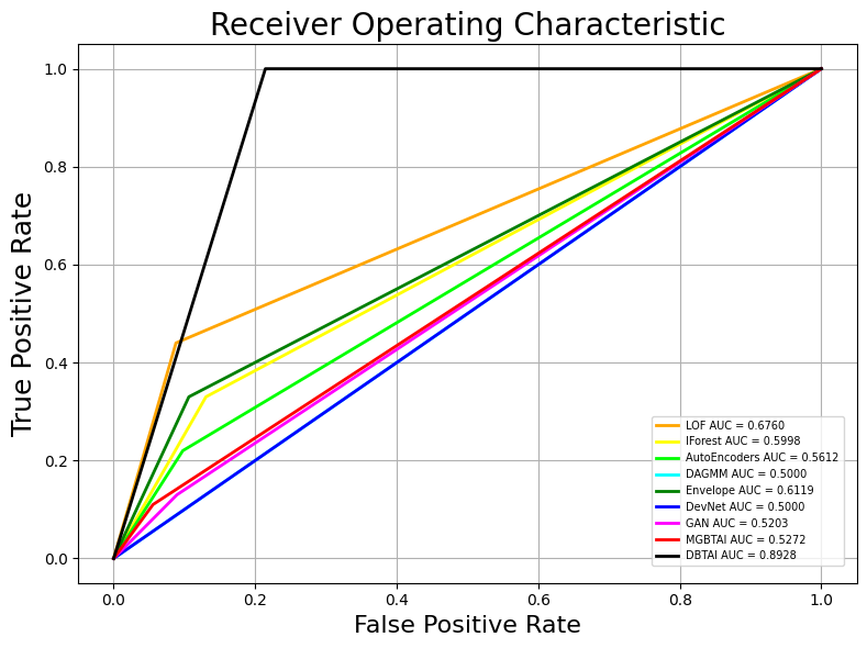
(a) glass

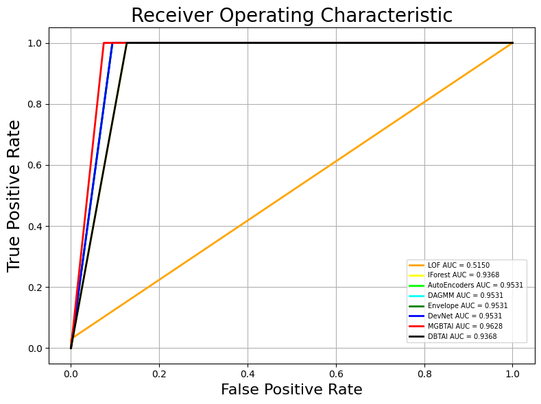
(b) http

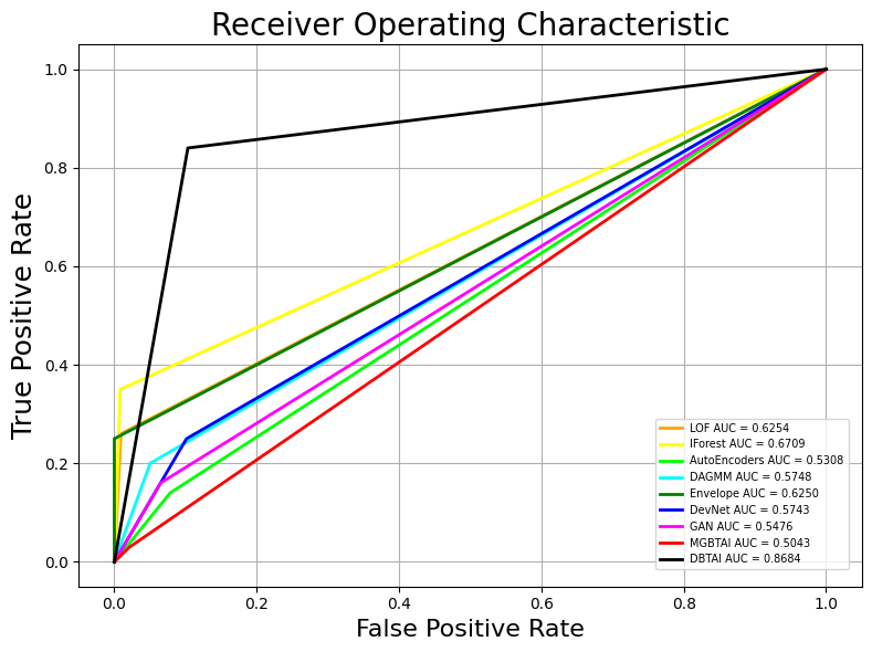
(c) Ionosphere

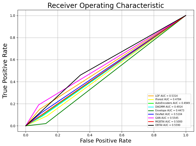
(d) landsat

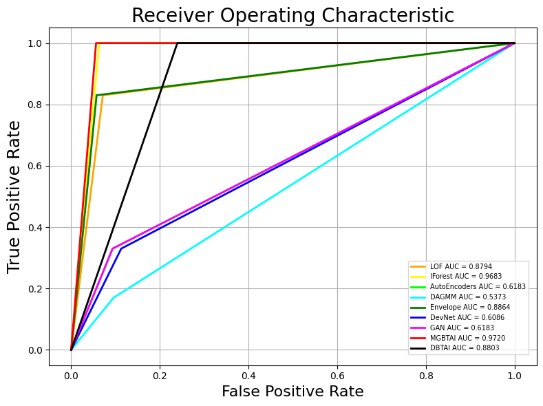
(e) Lymphography

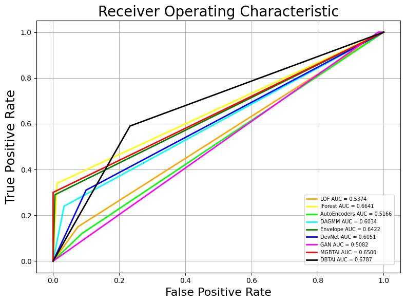
(f) satellite

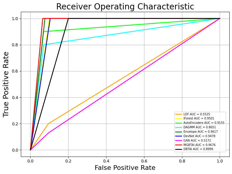
(a) WBC

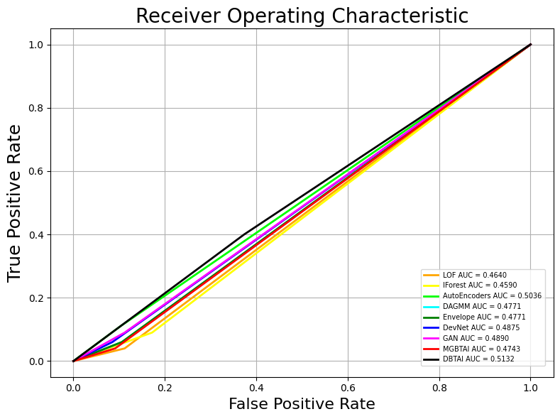
(b) WPBC

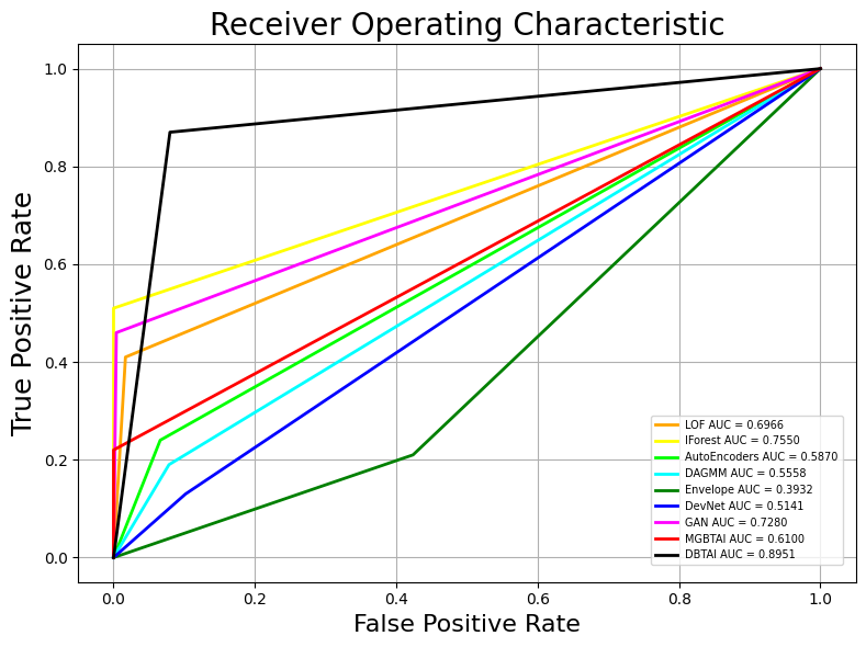
(c) MVTec-AD

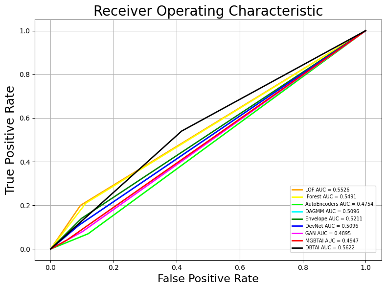
(d) Yelp

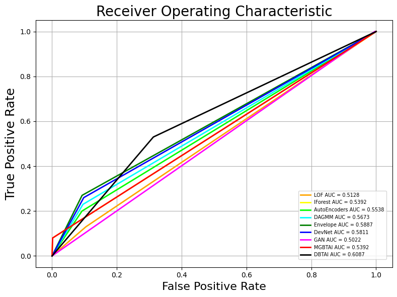
(e) SWaT2

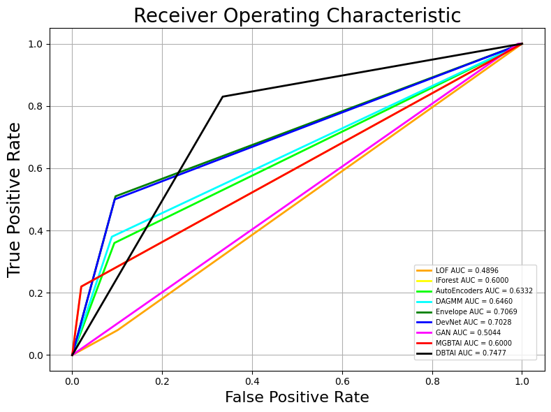
(f) SWaT5

Figure 6: AUC ROC comparison of Tree Based Approaches with other SOTA baselines for multivariate data

D.4 Univariate Results

MGBTAI stood out with perfect precision in 16 datasets, emerging as the top performer overall in 19 datasets. Following closely, d-BTAI achieved the highest precision in 18 datasets, with perfect precision in 11, highlighting its robust anomaly identification. Quantile-based algorithms (tanh, sigmoid, PEF) collectively excelled in 7 univariate datasets, showcasing their effectiveness. Notably, among quantile-based algorithms, sigmoid achieved the highest precision in 5 Univariate datasets. However, other algorithms (LOF, Iforest, Autoencoders, DAGMM, Envelope, DevNet, GAN) showed low performance, with only Autoencoders achieving the highest precision in one dataset, and other deep learning algorithms failing to achieve the highest precision for even one dataset as seen in Table 14

Table 15 shows that d-BTAI excels with perfect recall in 15 datasets, followed by MGBTAI with 12. Quantile-based algorithms (tanh, sigmoid, PEF) collectively achieve perfect recall in 16 datasets, highlighting their efficacy. Among them, PEF attains the highest recall in 20 Univariate datasets. Other algorithms (LOF, Iforest, Autoencoders, DAGMM, Envelope, DevNet, GAN) also perform well, demonstrating perfect recall in most datasets.

d-BTAI emerges as the top performer among 13 anomaly detection algorithms, achieving the highest F1-score overall and excelling in 19 univariate datasets, including perfect scores in 7. MGBTAI follows with the highest F1 score in 9 datasets. Together, d-BTAI and MGBTAI jointly provide the highest F1-score across the entire univariate dataset collection. Conversely, other algorithms (LOF, Iforest, Autoencoders, DAGMM, Envelope, DevNet, GAN) exhibit low performance, with only Autoencoders achieving the highest F1 score in one dataset. Quantile-based algorithms (tanh, sigmoid, PEF) collectively excel in 8 univariate datasets, with PEF achieving the highest F1 score in 5 among them as displayed in Table 16

In Table 17 we can see that d-BTAI emerges as the top performer among 13 anomaly detection algorithms, achieving the highest AUC-ROC overall and perfect scores in 15 datasets. MGBTAI closely follows,standing out in 12 datasets, with perfection in 11. Together, d-BTAI and MGBTAI jointly lead in AUC-ROC for 8 common datasets. Quantile algorithms (tanh, sigmoid, PEF) collectively excel, securing the highest AUC-ROC in 10 univariate datasets, emphasizing their effectiveness across diverse datasets. Additionally, the other algorithms (LOF, Iforest, Autoencoders, DAGMM, Envelope, DevNet, GAN) collectively displayed the highest AUC-ROC in 4 datasets.
The analysis of univariate results has been discussed in detail in section 3.4 of the main text.

D.5 Comparison Within Quantile-Based Algorithms

In this section we assessed the performance of q- LSTM with Tanh, Sigmoid, and PEF activation functions, alongside Deep Quantile Regression, across 31 univariate datasets. As seen in Table 18 Quantile LSTM(PEF) emerged as the top performer for 16 datasets. Quantile LSTM with tanh and sigmoid activation excelled in 5 datasets and the traditional Deep Quantile Regression on only 3 datasets as discussed in section 3.5 of the main text.

D.6 Experimenting with Parameterised Eliot Function(PEF)

In this section, we explore the application of the the PEF activation function in LSTM, GAN, and Autoencoders, alongside Deep Quantile Regression. A comprehensive comparison is conducted against the standard activation functions traditionally employed by these algorithms.

LSTM with standard activation functions tanh and sigmoid achieved excelled for 11 datasets whereas LSTM with PEF activation function achieved the highest recall for 10 datasets. Identical results observed for 10 datasets as displayed in 19

Deep Quantile Regression employing the PEF activation function achieved the highest recall for 14.Quantile Regression with tanh and sigmoid activations also emerged as a top-performing model achieving superior performance for 17 datasets as observed in Table 20.

GAN with standard activation functions like tanh and sigmoid achieved outperformed in 9 datasets whereas GAN with PEF activation function demonstrated superiority in only 3 datasets.GAN with PEF and GAN with standard activation functions generated identical results for 19 datasets as displayed in Table 21

Evaluation of Autoencoders using standard activation functions versus PEF activation function produced same results.

DATASET	SIZE	ANOMALIES	%ANOMALIES	DOMAIN
yahoo1	1420	2	0.14	Industrial
yahoo2	1461	8	0.55	Industrial
yahoo3	1439	8	0.56	Industrial
yahoo5	1421	9	0.63	Industrial
yahoo6	1421	4	0.28	Industrial
yahoo7	1680	11	0.65	Industrial
yahoo8	1680	10	0.60	Industrial
yahoo9	1680	8	0.48	Industrial
Speed_6005	2500	1	0.04	Non-Industrial
Speed_7578	1127	4	0.35	Non-Industrial
Speed_t4013	2495	2	0.08	Non-Industrial
TravelTime_387	2500	3	0.12	Non-Industrial
TravelTime_451	2162	1	0.05	Non-Industrial
Occupancy_6005	2380	1	0.04	Non-Industrial
Occupancy_t4013	2500	2	0.08	Non-Industrial
yahoo_syn1	1420	12	0.85	Industrial
yahoo_syn2	1461	18	1.23	Industrial
yahoo_syn3	1449	18	1.24	Industrial
yahoo_syn5	1431	19	1.33	Industrial
yahoo_syn6	1431	14	0.98	Industrial
yahoo_syn7	1690	21	1.24	Industrial
yahoo_syn8	1690	20	1.18	Industrial
yahoo_syn9	1690	18	1.07	Industrial
aws1	1049	1	0.10	Industrial
aws2	2486	2	0.08	Industrial
aws3	1499	1	0.07	Industrial
aws_syn1	1049	10	1.05	Industrial
aws_syn2	2486	20	0.88	Industrial
aws_syn3	1499	10	0.73	Industrial
Industrial_1	544	8	1.47	Industrial
Industrial_2	1609	3	0.19	Industrial

Table 13: Univariate Datasets Characterisation

Dataset	LOF	Iforest	Autoencoders	DAGMM	Envelope	DevNet	GAN	MGBTAI	d-BTAI	q-LSTM	q-LSTM	QReg	q-LSTM
										(tanh)	(sigmoid)		(PEF)
yahoo1	0.01	0.01	0.01	0.01	0.01	0.01	0.01	1	1	0.08	0.022	0	0.0465
yahoo2	0.06	0.04	0.05	0.05	0.05	0.06	0	1	0.89	0.015	0.22	0.1786	1
yahoo3	0.06	0.04	0.05	0.05	0.05	0.06	0	0.5	0.88	0.25	0.7778	0.1538	0.28
yahoo5	0.02	0.03	0.04	0.04	0.04	0	0	1	1	0.019	0.0092	0	0.022
yahoo6	0.03	0.02	0.03	0.03	0.03	0.03	0	1	1	0.027	0.0139	0.0028	0.0275
yahoo7	0.02	0.03	0	0.03	0.03	0.01	0.01	0.5	0.57	0.069	0.0732	0	0.066
yahoo8	0.01	0.01	0.01	0.01	0.01	0.01	0.01	1	1	0.029	0.0268	0	0.028
yahoo9	0.01	0.01	0.05	0.05	0.01	0.02	0	1	1	0.019	1	0.0049	0.0208
Speed_6005	0.01	0.004	0.004	0.004	0.004	NA	0.004	0.2	0.5	0.0138	0.0123	0	0.014
Speed_7578	0.03	0.03	0.03	0.04	0.03	0	0.04	0.09	0.25	0.5	0.5	0.5	0.086
Speed_t4013	0.02	0.01	0.01	0	0.01	0	0.01	0.29	0.67	0.0078	0.0344	0.0392	0.053
TravelTime_387	0.01	0.01	0.01	0.01	0.01	0.01	0	0.05	0.33	0.0069	0.0041	0.0011	0.011
TravelTime_451	0.005	0.004	0.005	0.005	0.005	NA	0	0.04	0.09	0	0.007	0	0.006
Occupancy_6005	0.004	0.004	0.004	0.004	0.004	NA	0	0.06	1	0.0116	0.0109	0	0.03
Occupancy_t4013	0.01	0.01	0.01	0	0.01	NA	0	0.33	1	0.0869	0.0076	0.0038	0.06
yahoo_syn1	0.08	0.06	0.08	0.08	0.08	0.08	0	1	1	0.087	0.0816	0.0303	0.375
yahoo_syn2	0.13	0.1	0.12	0.12	0.13	0.14	0	1	0.94	1	0.0243	0	1
yahoo_syn3	0.1	0.1	0.11	0.11	0.11	0.14	0	0.81	0.89	0.061	1	0.0805	0.6
yahoo_syn5	0.08	0.09	0.11	0.11	0.11	0	0.01	1	0.48	0.055	0.0394	0	0.0625
yahoo_syn6	0.03	0.08	0.03	0.03	0.03	0.03	0.01	1	0.25	0.043	0.0606	0.0098	0.764
yahoo_syn7	0.04	0.07	0.05	0.07	0.08	0.1	0.01	0.56	0.24	0.2	0.26	0.0092	0.411
yahoo_syn8	0.03	0.02	0.02	0	0.02	0.02	0.01	1	0.1	0.07	0.0714	0.2	0.197
yahoo_syn9	0.11	0.08	0.11	0.03	0.1	0.11	0	1	1	0.116	1	0.0102	1
aws1	0.01	0.01	0.01	0.01	0.01	NA	0	1	0.1	0.036	0.0278	0.0204	0.041
aws2	0.09	0.01	0	0	0.04	0.01	0	1	0.18	0.005	0.0147	0	0.0042
aws3	0.01	0.01	0.01	0.01	0.01	NA	0	0.5	0.07	0.006	0.0083	0.0116	0.0181
aws_syn1	0.0952	0.0324	0	0.08	0.0599	0.0283	0	0.9	0.91	0.224	0.0843	0.0204	0.0843
aws_syn2	0.0241	0.0694	0	0.08	0.0797	0.004	0.008	0.67	0.52	0.049	0.0424	0	0.0042
aws_syn3	0.0667	0.0526	0.0133	0.07	0.0617	0.0213	0	0.9	0.9	1	0.0603	0.0116	0.0603
Industrial_1	0.1538	0.0167	0.014	0	0.0099	0.0203	0	1	1	0.019	0.028	0	0.357
Industrial_2	0.0341	0.0167	1	0.0148	0.0099	0.0203	0	1	1	1	1	0.0148	1

Table 14: Precision values of the 13 algorithms on the 31 univariate datasets. The highest value(s) is marked in bold. NA implies that DevNet cannot be run on those datasets since they have less than 2 anomalies.

Dataset	LOF	Iforest	Autoencoders	DAGMM	Envelope	DevNet	GAN	MGBTAI	d-BTAI	q-LSTM	q-LSTM	QReg	q-LSTM
										(tanh)	(sigmoid)		(PEF)
yahoo1	1	1	1	1	1	1	0.5	1	1	1	1	0	1
yahoo2	1	1	1	1	1	1	0	0.25	1	0.25	0.625	0.625	0.375
yahoo3	1	1	1	0.88	0.88	1	0	0.88	0.88	1	0.875	0.75	1
yahoo5	0.33	0.67	0.67	0.67	0.67	0	0	0.33	0.33	0.67	0.333	0	0.66
yahoo6	1	1	1	1	1	1	1	1	1	1	1	1	1
yahoo7	0.36	0.55	0	0.45	0.45	0.09	1	0.36	0.36	0.3636	0.545	0	0.54
yahoo8	0.2	0.2	0.1	0.2	0.2	0.2	1	0.01	0.1	0.3	0.3	0	0.3
yahoo9	0.2	0.2	1	1	0.2	0.38	0	0.62	1	0.625	0.75	0.875	0.75
Speed_6005	1	1	1	1	1	NA	1	1	1	1	1	0	1
Speed_7578	0.75	1	1	1	1	0	1	0.75	0.5	0.25	0.25	0.24	1
Speed_t4013	1	1	1	1	1	0	1	1	1	1	1	1	1
TravelTime_387	0.67	0.67	0.67	0.67	0.67	0.67	0	0.67	0.33	0.33	0.33	0.33	0.67
TravelTime_451	1	1	1	1	1	NA	0	1	1	0	1	0	1
Occupancy_6005	1	1	1	1	1	1	0	1	1	1	1	0	1
Occupancy_t4013	1	1	1	0	1	NA	0	1	1	1	1	1	1
yahoo_syn1	1	1	1	1	1	1	0	0.17	1	1	1	0.0833	1
yahoo_syn2	1	1	1	1	1	1	0	0.28	0.94	0.5	0.611	0	0.611
yahoo_syn3	0.83	1	0.94	0.94	1	1	0	0.72	0.94	0.6111	0.444	0.3889	1
yahoo_syn5	0.58	0.84	0.84	0.84	0.84	0	1	0.42	0.53	0.7368	0.737	0	0.578
yahoo_syn6	0.29	1	0.29	0.29	0.29	0.29	1	0.29	0.29	0.8571	0.857	1	0.928
yahoo_syn7	0.33	0.71	0.43	0.52	0.67	0.71	1	0.24	0.24	0.619	0.619	0.1905	0.66
yahoo_syn8	0.25	0.2	0.15	0	0.15	0.2	1	0.05	0.1	0.4	0.4	1	0.7
yahoo_syn9	1	1	1	0.25	1	1	0	0.06	1	0.2778	0.722	0.8889	0.94
aws1	1	1	1	1	1	NA	0	1	1	1	1	1	1
aws2	1	1	1	1	1	1	0	0.5	1	1	1	0	1
aws3	1	1	1	1	1	NA	0	1	1	1	1	1	1
aws_syn1	0.045	1	0	0.82	1	0.3	0	0.9	1	1	0.636	1	1
aws_syn2	0.0241	1	0	1	1	0.05	1	1	0.55	1	0.864	0	1
aws_syn3	0.067	1	0.2	1	1	0.3	0	0.9	0.9	1	0.636	1	1
Industrial_1	0.1538	1	1	0	1	1	0	1	0.23	0.66	0.66	0	1
Industrial_2	0.0341	1	1	1	1	1	0	1	0.88	1	1	1	1

Table 15: Recall values of the 13 algorithms on the 31 univariate datasets. The highest value(s) is marked in bold.

Dataset	LOF	Iforest	Autoencoders	DAGMM	Envelope	DevNet	GAN	MGBTAI	d-BTAI	q-LSTM	q-LSTM	QReg	q-LSTM
										(tanh)	(sigmoid)		(PEF)
yahoo1	0.03	0.02	0.01	0.03	0.03	0.03	0.01	1	1	0.1481	0.043	0	0.0889
yahoo2	0.11	0.08	0.1	0.1	0.1	0.12	0	0.4	0.94	0.0282	0.325	0.2778	0.5455
yahoo3	0.11	0.09	0.1	0.09	0.09	0.11	0	0.64	0.88	0.4000	0.8235	0.2553	0.4375
yahoo5	0.04	0.06	0.08	0.08	0.08	0	0	0.5	0.5	0.0374	0.0179	0	0.0426
yahoo6	0.05	0.04	0.05	0.05	0.06	0.05	0.01	1	1	0.0526	0.0275	0.0056	0.0535
yahoo7	0.04	0.05	0	0.06	0.05	0.01	0.01	0.42	0.44	0.1159	0.129	0	0.1176
yahoo8	0.02	0.02	0.01	0.02	0.02	0.02	0.01	0.01	0.18	0.0526	0.0492	0	0.0512
yahoo9	0.02	0.02	0.09	0.09	0.02	0.03	0	0.77	1	0.0362	0.8571	0.0098	0.0405
Speed_6005	0.03	0.01	0.01	0.01	0.01	0	0.01	0.33	0.67	0.0273	0.0243	0	0.0276
Speed_7578	0.06	0.06	0.06	0.07	0.06	0	0.07	0.16	0.33	0.33	0.33	0.32	0.1584
Speed_t4013	0.04	0.01	0.01	0.01	0.02	0	0.01	0.44	0.8	0.0155	0.0666	0.0755	0.1007
TravelTime_387	0.02	0.01	0.02	0.02	0.02	0.02	0	0.09	0.33	0.0135	0.0089	0.0021	0.0216
TravelTime_451	0.01	0.01	0.01	0.01	0.01	0	0	0.08	0.17	0	0.0139	0	0.0119
Occupancy_6005	0.01	0.01	0.01	0.01	0.01	0.01	0	0.12	1	0.0229	0.0217	0	0.0583
Occupancy_t4013	0.02	0.01	0.02	0	0.02	0.02	0	0.5	1	0.16	0.0152	0.0076	0.1132
yahoo_syn1	0.16	0.12	0.16	0.16	0.14	0.16	0	0.29	1	0.1600	0.1509	0.0444	0.5455
yahoo_syn2	0.23	0.18	0.21	0.22	0.23	0.24	0	0.43	0.94	0.6667	0.0467	0	0.7585
yahoo_syn3	0.18	0.18	0.2	0.2	0.2	0.24	0	0.76	0.92	0.1111	0.6154	0.1333	0.75
yahoo_syn5	0.14	0.17	0.2	0.2	0.2	0	0.03	0.59	0.5	0.1022	0.0749	0	0.1128
yahoo_syn6	0.05	0.15	0.05	0.05	0.05	0.05	0.02	0.44	0.27	0.0825	0.1132	0.0194	0.8381
yahoo_syn7	0.07	0.13	0.09	0.012	0.15	0.17	0.02	0.33	0.24	0.3023	0.3662	0.0176	0.5066
yahoo_syn8	0.05	0.04	0.03	0	0.03	0.04	0.02	0.1	0.1	0.1194	0.1212	0.34	0.3075
yahoo_syn9	0.19	0.15	0.19	0.05	0.18	0.19	0	0.11	1	0.1639	0.8387	0.0202	0.9691
aws1	0.02	0.02	0.02	0.02	0.02	0.02	0	1	0.18	0.0690	0.0541	0.04	0.0788
aws2	0.17	0.02	0	0.01	0.08	0.02	0	0.67	0.31	0.0092	0.029	0	0.0084
aws3	0.01	0.01	0.01	0.01	0.01	0.01	0	0.67	0.13	0.0123	0.0164	0.023	0.0356
aws_syn1	0.1739	0.0627	0	0.14	0.113	0.0517	0	0.9	0.95	0.3667	0.1489	0.04	0.9888
aws_syn2	0.0496	0.1299	0	0.15	0.1476	0.0074	0.0159	0.8	0.54	0.0934	0.0809	0	0.9045
aws_syn3	0.125	0.1	0.025	0.12	0.1163	0.0397	0	0.9	0.9	1	0.1102	0.023	0.9818
Industrial_1	0.2667	0.0328	0.0276	0	0.0195	0.0397	0	1	0.375	0.038	0.054	0	0.0689
Industrial_2	0.0659	0.0328	1	0.0291	0.0195	0.0397	0	1	0.94	1	1	0.029	1

Table 16: F1 Score values of the 13 algorithms on the 31 univariate datasets. The highest value(s) is marked in bold.

Dataset	LOF	Iforest	Autoencoders	DAGMM	Envelope	DevNet	GAN	MGBTAI	d-BTAI	q-LSTM	q-LSTM	QReg	q-LSTM
										(tanh)	(sigmoid)		(PEF)
yahoo1	0.95	0.94	0.9	0.95	0.95	0.95	0.7	1	1	0.992	0.9686	0.4908	0.9855
yahoo2	0.95	0.94	0.95	0.95	0.95	0.96	0.45	0.62	1	0.58	0.84	0.8046	0.6875
yahoo3	0.95	0.94	0.95	0.89	0.89	0.95	0.45	0.94	0.94	0.992	0.9367	0.8634	0.994
yahoo5	0.62	0.77	0.78	0.78	0.78	0.45	0.45	0.67	0.67	0.725	0.5496	0.4865	0.7364
yahoo6	0.95	0.94	0.95	0.95	0.95	0.95	0.5	1	1	0.949	0.8998	0.5	0.95
yahoo7	0.63	0.71	0.45	0.68	0.68	0.5	0.5	0.68	0.68	0.666	0.7499	0.4889	0.7448
yahoo8	0.55	0.54	0.5	0.55	0.55	0.55	0.5	0.5	0.55	0.62	0.6172	0.4892	0.6188
yahoo9	0.55	0.54	0.95	0.95	0.55	0.63	0.45	0.81	1	0.734	0.875	0.5139	0.7905
Speed_6005	0.99	0.95	0.95	0.93	0.95	NA	0.94	1	1	0.9857	0.9839	0.4577	0.9718
Speed_7578	0.83	0.94	0.95	0.95	0.95	0.45	0.95	0.86	0.75	0.6240	0.62400	0.6121	0.981
Speed_t4013	0.98	0.94	0.93	0.91	0.95	0.46	0.94	1	1	0.9492	0.989	0.9902	0.9928
TravelTime_387	0.78	0.77	0.78	0.78	0.79	0.78	0.45	0.83	0.67	0.638	0.618	0.4782	0.7988
TravelTime_451	0.95	0.94	0.95	0.95	0.95	NA	0.45	0.99	1	0.496	0.967	0.4903	0.9616
Occupancy_6005	0.95	0.94	0.95	0.95	0.95	0.95	0.45	1	1	0.9821	0.9810	0.4891	0.9932
Occupancy_t4013	0.95	0.94	0.95	0.5	0.95	NA	0.45	1	1	0.9957	0.9480	0.895	0.9937
yahoo_syn1	0.95	0.94	0.95	0.95	0.95	0.95	0.45	0.58	1	0.955	0.952	0.5303	0.9928
yahoo_syn2	0.96	0.94	0.95	0.95	0.96	0.96	0.45	0.64	0.97	0.75	0.652	0.4903	0.8055
yahoo_syn3	0.87	0.94	0.93	0.93	0.95	0.96	0.45	0.86	0.97	0.747	0.722	0.6664	0.9958
yahoo_syn5	0.74	0.87	0.88	0.88	0.88	0.45	0.5	0.71	0.76	0.783	0.748	0.4908	0.7306
yahoo_syn6	0.59	0.94	0.59	0.59	0.6	0.59	0.5	0.64	0.64	0.835	0.863	0.5	0.9625
yahoo_syn7	0.62	0.8	0.67	0.71	0.79	0.82	0.5	0.62	0.61	0.794	0.798	0.4662	0.824
yahoo_syn8	0.58	0.54	0.52	0.5	0.52	0.55	0.5	0.53	0.54	0.668	0.669	0.65	0.8329
yahoo_syn9	0.95	0.94	0.95	0.58	0.95	0.95	0.45	0.53	1	0.628	0.861	0.4789	0.97
aws1	0.95	0.94	0.95	0.95	0.95	NA	0.45	1	1	0.987	0.9832	0.977	0.9888
aws2	1	0.96	0.75	0.86	0.99	0.96	0.41	0.75	1	0.913	0.973	0.4895	0.9045
aws3	0.95	0.94	0.95	0.95	0.95	NA	0.45	1	1	0.946	0.9596	0.9716	0.9818
aws_syn1	0.9543	0.8788	0.449	0.85	0.9363	0.85	0.4494	0.95	1	0.983	0.785	0.977	0.9833
aws_syn2	0.6007	0.9457	0.449	0.95	0.9532	0.95	0.5	1	0.77	0.921	0.853	0.489	0.9211
aws_syn3	0.953	0.9396	0.55	0.95	0.949	0.95	0.4492	0.95	0.95	1	0.785	0.9716	1
Industrial_1	0.9589	0.5605	0.93	0.45	0.553	0.45	0.41	1	0.975	0.5803	0.6604	0.48	0.9865
Industrial_2	0.995	0.945	1	0.0148	0.9065	0.9378	0.41	1	0.9998	1	1	0.9378	1

Table 17: AUC-ROC values of the 13 algorithms on the 31 univariate datasets. The highest value(s) is marked in bold.

Dataset	q-LSTM(tanh)				q-LSTM(sigmoid)				Deep Quantile Regression				Quantile LSTM(PEF)
	Precision	Recall	F1 Score	AUC-ROC	Precision	Recall	F1 Score	AUC-ROC	Precision	Recall	F1 Score	AUC-ROC	Precision	Recall	F1 Score	AUC-ROC
yahoo1	0.08	1	0.1481	0.992	0.022	1	0.043	0.9686	0	0	0	0.4908	0.0465	1	0.0889	0.9855
yahoo2	0.015	0.25	0.0282	0.58	0.22	0.625	0.325	0.84	0.1786	0.625	0.2778	0.8046	1	0.375	0.5455	0.6875
yahoo3	0.25	1	0.4	0.992	0.7778	0.875	0.8235	0.9367	0.1538	0.75	0.2553	0.8634	0.28	1	0.4375	0.994
yahoo5	0.019	0.67	0.0374	0.725	0.0092	0.333	0.0179	0.5496	0	0	0	0.4865	0.022	0.66	0.0426	0.7364
yahoo6	0.027	1	0.0526	0.949	0.0139	1	0.0275	0.8998	0.0028	1	0.0056	0.5	0.0275	1	0.0535	0.95
yahoo7	0.069	0.3636	0.1159	0.666	0.0732	0.545	0.129	0.7499	0	0	0	0.4889	0.066	0.54	0.1176	0.7448
yahoo8	0.029	0.3	0.0526	0.62	0.0268	0.3	0.0492	0.6172	0	0	0	0.4892	0.028	0.3	0.0512	0.6188
yahoo9	0.019	0.625	0.0362	0.734	1	0.75	0.8571	0.875	0.0049	0.875	0.0098	0.5139	0.0208	0.75	0.0405	0.7905
Speed_6005	0.0138	1	0.0273	0.9857	0.0123	1	0.0243	0.9839	0	0	0	0.4577	0.014	1	0.0276	0.9718
Speed_7578	0.5	0.25	0.33	0.624	0.5	0.25	0.33	0.624	0.5	0.24	0.32	0.6121	0.086	1	0.1584	0.981
Speed_t4013	0.0078	1	0.0155	0.9492	0.0344	1	0.0666	0.989	0.0392	1	0.0755	0.9902	0.053	1	0.1007	0.9928
TravelTime_387	0.0069	0.33	0.0135	0.638	0.0041	0.33	0.0089	0.618	0.0011	0.3333	0.0021	0.4782	0.011	0.67	0.0216	0.7988
TravelTime_451	0	0	0	0.496	0.007	1	0.0139	0.967	0	0	0	0.4903	0.006	1	0.0119	0.9616
Occupancy_6005	0.0116	1	0.0229	0.9821	0.0109	1	0.0217	0.981	0	0	0	0.4891	0.03	1	0.0583	0.9932
Occupancy_t4013	0.0869	1	0.16	0.9957	0.0076	1	0.0152	0.948	0.0038	1	0.0076	0.895	0.06	1	0.1132	0.9937
yahoo_syn1	0.087	1	0.16	0.955	0.0816	1	0.1509	0.952	0.0303	0.0833	0.0444	0.5303	0.375	1	0.5455	0.9928
yahoo_syn2	1	0.5	0.6667	0.75	0.0243	0.611	0.0467	0.652	0	0	0	0.4903	1	0.611	0.7585	0.8055
yahoo_syn3	0.061	0.6111	0.1111	0.747	1	0.444	0.6154	0.722	0.0805	0.3889	0.1333	0.6664	0.6	1	0.75	0.9958
yahoo_syn5	0.055	0.7368	0.1022	0.783	0.0394	0.737	0.0749	0.748	0	0	0	0.4908	0.0625	0.578	0.1128	0.7306
yahoo_syn6	0.043	0.8571	0.0825	0.835	0.0606	0.857	0.1132	0.863	0.0098	1	0.0194	0.5	0.764	0.928	0.8381	0.9625
yahoo_syn7	0.2	0.619	0.3023	0.794	0.26	0.619	0.3662	0.798	0.0092	0.1905	0.0176	0.4662	0.411	0.66	0.5066	0.824
yahoo_syn8	0.07	0.4	0.1194	0.668	0.0714	0.4	0.1212	0.669	0.2	1	0.34	0.65	0.197	0.7	0.3075	0.8329
yahoo_syn9	0.116	0.2778	0.1639	0.628	1	0.722	0.8387	0.861	0.0102	0.8889	0.0202	0.4789	1	0.94	0.9691	0.97
aws1	0.036	1	0.069	0.987	0.0278	1	0.0541	0.9832	0.0204	1	0.04	0.977	0.041	1	0.0788	0.9888
aws2	0.005	1	0.0092	0.913	0.0147	1	0.029	0.973	0	0	0	0.4895	0.0042	1	0.0084	0.9045
aws3	0.006	1	0.0123	0.946	0.0083	1	0.0164	0.9596	0.0116	1	0.023	0.9716	0.0181	1	0.0356	0.9818
aws_syn1	0.224	1	0.3667	0.983	0.0843	0.636	0.1489	0.785	0.0204	1	0.04	0.977	0.224	1	0.366	0.9833
aws_syn2	0.049	1	0.0934	0.921	0.0424	0.864	0.0809	0.853	0	0	0	0.4895	0.0489	1	0.0932	0.9211
aws_syn3	1	1	1	1	0.0603	0.636	0.1102	0.785	0.0116	1	0.023	0.9716	1	1	1	1
Industrial_1	0.019	0.66	0.038	0.5803	0.028	0.66	0.054	0.6604	0	0	0	0.48	0.357	1	0.0689	0.9865
Industrial_2	1	1	1	1	1	1	1	1	0.0148	1	0.029	0.9378	1	1	1	1

Table 18: Performance of Quantile LSTM with activation functions tanh, sigmoid, and PEF activation function along with Deep Quantile Regression on 31 univariate datasets. The best performing algorithm(s) is marked in bold.

Dataset	LSTM				LSTM(PEF)
	Precision	Recall	F1 Score	AUC-ROC	Precision	Recall	F1 Score	AUC-ROC
yahoo1	0.007	0.5	0.0139	0.7002	0.007	0.5	0.0139	0.7002
yahoo2	0.0411	0.75	0.0779	0.8267	0.0411	0.75	0.0779	0.8267
yahoo3	0.0417	0.75	0.0789	0.8267	0.0486	0.875	0.0921	0.8895
yahoo5	0.0141	0.2222	0.0265	0.5614	0.0352	0.5556	0.0662	0.7292
yahoo6	0.0141	0.5	0.0274	0.7005	0.0211	0.75	0.0411	0.8258
yahoo7	0.0119	0.1818	0.0223	0.5411	0.006	0.0909	0.0112	0.4953
yahoo8	0.0119	0.2	0.0225	0.5502	0.006	0.1	0.0112	0.4999
yahoo9	0.0119	0.25	0.0227	0.5753	0	0	0	0.4497
Speed_6005	0.004	1	0.0079	0.9497	0	0	0	0.4499
Speed_7578	0.0254	0.75	0.0492	0.8237	0.0263	0.75	0.0508	0.8254
Speed_t4013	0.0079	1	0.0156	0.9494	0.0078	1	0.0156	0.9492
TravelTime_387	0	0	0	0.4499	0.004	0.3333	0.0079	0.6167
TravelTime_451	0	0	0	0.45	0	0	0	0.45
Occupancy_6005	0.0042	1	0.0084	0.9501	0.0042	1	0.0084	0.9501
Occupancy_t4013	0.008	1	0.0159	0.9503	0.008	1	0.0159	0.9503
yahoo_syn1	0.0211	0.25	0.039	0.5755	0.0282	0.3333	0.0519	0.6176
yahoo_syn2	0.0411	0.3333	0.0732	0.6181	0.0479	0.3889	0.0854	0.6462
yahoo_syn3	0.0479	0.3889	0.0854	0.6458	0.0548	0.4444	0.0976	0.6739
yahoo_syn5	0.0208	0.1579	0.0368	0.5289	0.0278	0.2105	0.0491	0.5556
yahoo_syn6	0.0278	0.2857	0.0506	0.5934	0.0278	0.2857	0.0506	0.5934
yahoo_syn7	0.0118	0.0118	0.0209	0.4972	0.0059	0.0476	0.0105	0.4731
yahoo_syn8	0.0118	0.1	0.0211	0.4996	0.0059	0.05	0.0105	0.4743
yahoo_syn9	0.0176	0.1667	0.0319	0.5333	0.0059	0.0556	0.0106	0.4771
aws1	0.0094	1	0.0187	0.9498	0.0094	1	0.0187	0.9498
aws2	0.0032	0.5	0.0063	0.6865	0.0032	0.5	0.0076	0.6978
aws3	0.0067	1	0.0132	0.9502	0	0	0	0.4498
aws_syn1	0.0935	1	0.1709	0.9533	0.0935	1	0.1709	0.9533
aws_syn2	0.0249	1	0.0486	0.8412	0.0176	1	0.0345	0.7733
aws_syn3	0.0667	1	0.125	0.953	0.0667	1	0.125	0.953
Industrial_1	0.014	1	0.0276	0.9343	0	0	0	0.42
Industrial_2	0.0976	1	0.1778	0.931	0.11	0.75	0.19	0.83

Table 19: A Comparative Study of LSTM versus LSTM Using PEF Activation Function on 31 univariate datasets. The best performing algorithm(s) is marked in bold.

Dataset	Deep Quantile Regression				Deep Quantile Regression(PEF)
	Precision	Recall	F1 Score	AUC-ROC	Precision	Recall	F1 Score	AUC-ROC
yahoo1	0	0	0	0.4908	0.0014	1	0.0028	0.5
yahoo2	0.1786	0.625	0.2778	0.8046	0.0055	1	0.0109	0.5
yahoo3	0.1538	0.75	0.2553	0.8634	0.0169	0.125	0.0299	0.5422
yahoo5	0	0	0	0.4865	0.0143	0.444	0.0278	0.6246
yahoo6	0.0028	1	0.0056	0.5	0.0032	0.75	0.0063	0.5423
yahoo7	0	0	0	0.4889	0.0104	0.1818	0.0196	0.5336
yahoo8	0	0	0	0.4892	0.008	0.8	0.0158	0.6022
yahoo9	0.0049	0.875	0.0098	0.5139	0	0	0	0.4892
Speed_6005	0	0	0	0.4577	0	0	0	0.3684
Speed_7578	0.5	0.25	0.32	0.6121	0.0022	0.25	0.0044	0.4241
Speed_t4013	0.0392	1	0.0755	0.9902	0.0009	0.5	0.0018	0.5275
TravelTime_387	0.0011	0.3333	0.0021	0.4782	0.0037	0.3333	0.0073	0.6123
TravelTime_451	0	0	0	0.4903	0	0	0	0.4541
Occupancy_6005	0	0	0	0.4891	0	0	0	0.4901
Occupancy_t4013	0.0038	1	0.0076	0.895	0.0208	0.5	0.04	0.7406
yahoo_syn1	0.0303	0.0833	0.0444	0.5303	0.0085	1	0.0168	0.5
yahoo_syn2	0	0	0	0.4903	0.0123	1	0.0244	0.5
yahoo_syn3	0.0805	0.3889	0.1333	0.664	0.0521	0.2778	0.0877	0.607
yahoo_syn5	0	0	0	0.4908	0.0269	0.2632	0.0488	0.5673
yahoo_syn6	0.0098	1	0.0194	0.5	0.0117	0.2143	0.0222	0.5177
yahoo_syn7	0.0092	0.1905	0.0176	0.4662	0.023	0.0952	0.037	0.5221
yahoo_syn8	0.2	1	0.34	0.65	0.0147	0.05	0.0227	0.5049
yahoo_syn9	0.0102	0.8889	0.0202	0.4789	0	0	0	0.4901
aws1	0.0204	1	0.04	0.977	0	0	0	0.4167
aws2	0	0	0	0.4895	0.0008	1	0.0016	0.5
aws3	0.0116	1	0.023	0.9716	0.0027	1	0.0054	0.8776
aws_syn1	0.0204	0.1	0.0339	0.5268	0.0238	0.1	0.0385	0.5302
aws_syn2	0.0217	0.05	0.0303	0.5159	0.0081	1	0.016	0.5
aws_syn3	0	0	0	0.4872	0.0116	0.1	0.0208	0.5214
Industrial_1	0	0	0	0.4832	0	0	0	0.4454
Industrial_2	0.0148	1	0.029	0.9378	0.0148	1	0.0291	0.5

Table 20: A Comparative Study of Quantile regression using Standard Activation Functions versus PEF Activation Function on 31 univariate datasets. The best performing algorithm(s) is marked in bold.

Dataset	GAN				GAN(PEF)
	Precision	Recall	F1 Score	AUC-ROC	Precision	Recall	F1 Score	AUC-ROC
yahoo1	0.01	0.5	0.01	0.7	0	0	0	0.45
yahoo2	0	0	0	0.45	0	0	0	0.45
yahoo3	0	0	0	0.45	0	0	0	0.45
yahoo5	0	0	0	0.45	0	0	0	0.45
yahoo6	0	1	0.01	0.5	0	0	0	0.45
yahoo7	0.01	1	0.01	0.5	0.04	0.64	0.08	0.77
yahoo8	0.01	1	0.01	0.5	0	0	0	0.45
yahoo9	0	0	0	0.45	0.03	0.63	0.06	0.76
Speed_6005	0	1	0.01	0.94	0.00	1	0.01	0.94
Speed_7578	0.04	1	0.07	0.95	0.04	1	0.07	0.95
Speed_t4013	0.01	1	0.01	0.94	0	0	0	0.45
TravelTime_387	0	0	0	0.45	0	0	0	0.45
TravelTime_451	0	0	0	0.45	0	0	0	0.45
Occupancy_6005	0	0	0	0.45	0	0	0	0.45
Occupancy_t4013	0	0	0	0.45	0	0	0	0.45
yahoo_syn1	0	0	0	0.45	0	0	0	0.45
yahoo_syn2	0	0	0	0.45	0	0	0	0.45
yahoo_syn3	0	0	0	0.45	0	0	0	0.45
yahoo_syn5	0.01	1	0.03	0.5	0	0	0	0.45
yahoo_syn6	0.01	1	0.02	0.5	0	0	0	0.45
yahoo_syn7	0.01	1	0.02	0.5	0.04	0.33	0.07	0.62
yahoo_syn8	0.01	1	0.02	0.5	0	0	0	0.45
yahoo_syn9	0	0	0	0.45	0.02	0.17	0.03	0.53
aws1	0	0	0	0.45	0	0	0	0.45
aws2	0	0	0	0.41	0	0	0	0.41
aws3	0	0	0	0.45	0	0	0	0.45
aws_syn1	0	0	0	0.45	0	0	0	0.45
aws_syn2	0	0	0	0.41	0	0	0	0.41
aws_syn3	0	0	0	0.45	0	0	0	0.45
Industrial_1	0	0	0	0.41	0	0	0	0.41
Industrial_2	0	0	0	0.41	0.13	1	0.23	0.95

Table 21: A Comparative Study of GAN using Standard Activation Functions versus PEF Activation Function on 31 univariate datasets. The best performing algorithm(s) is marked in bold.

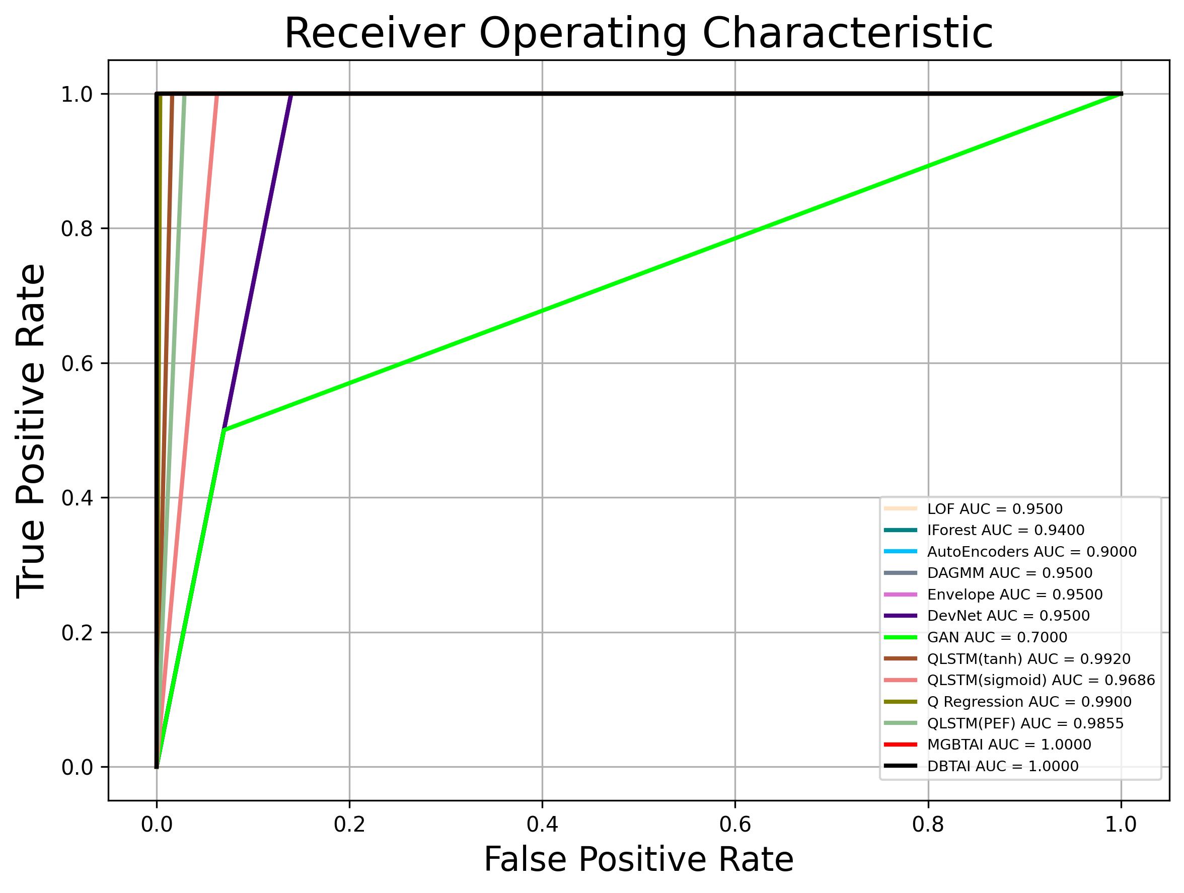
(a) yahoo1

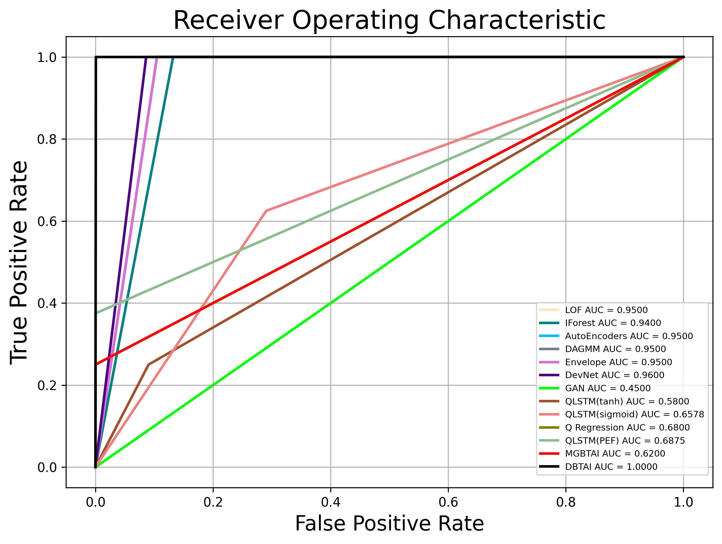
(b) yahoo2

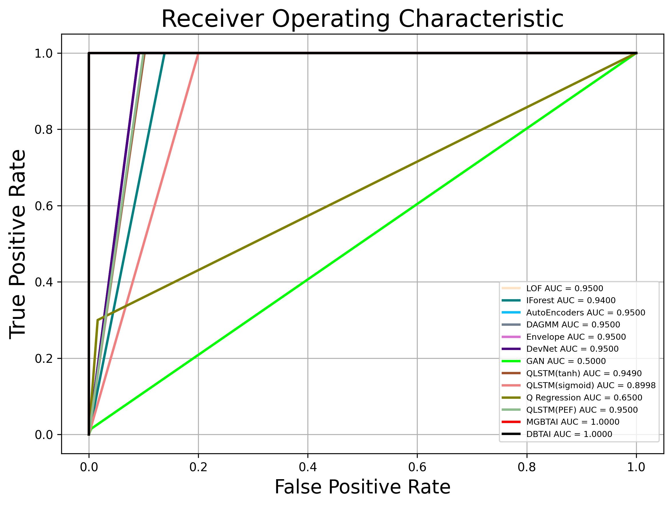
(c) yahoo6

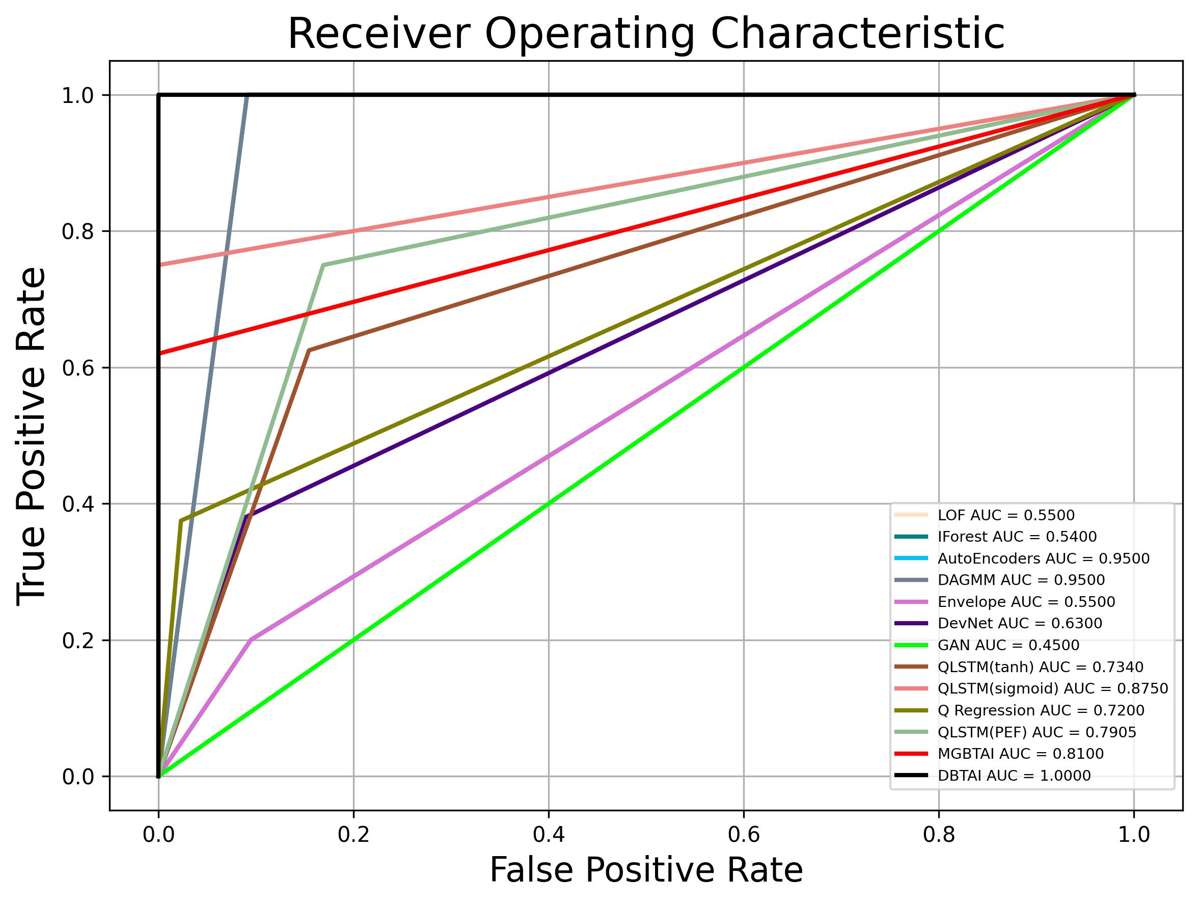
(d) yahoo9

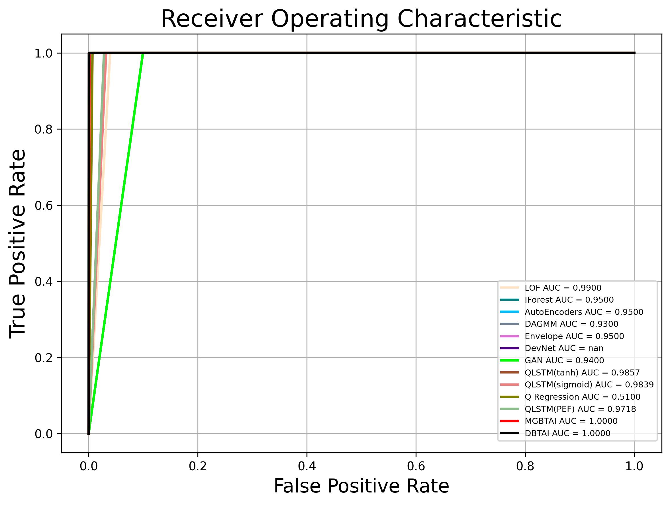
(e) Speed$\_$6005

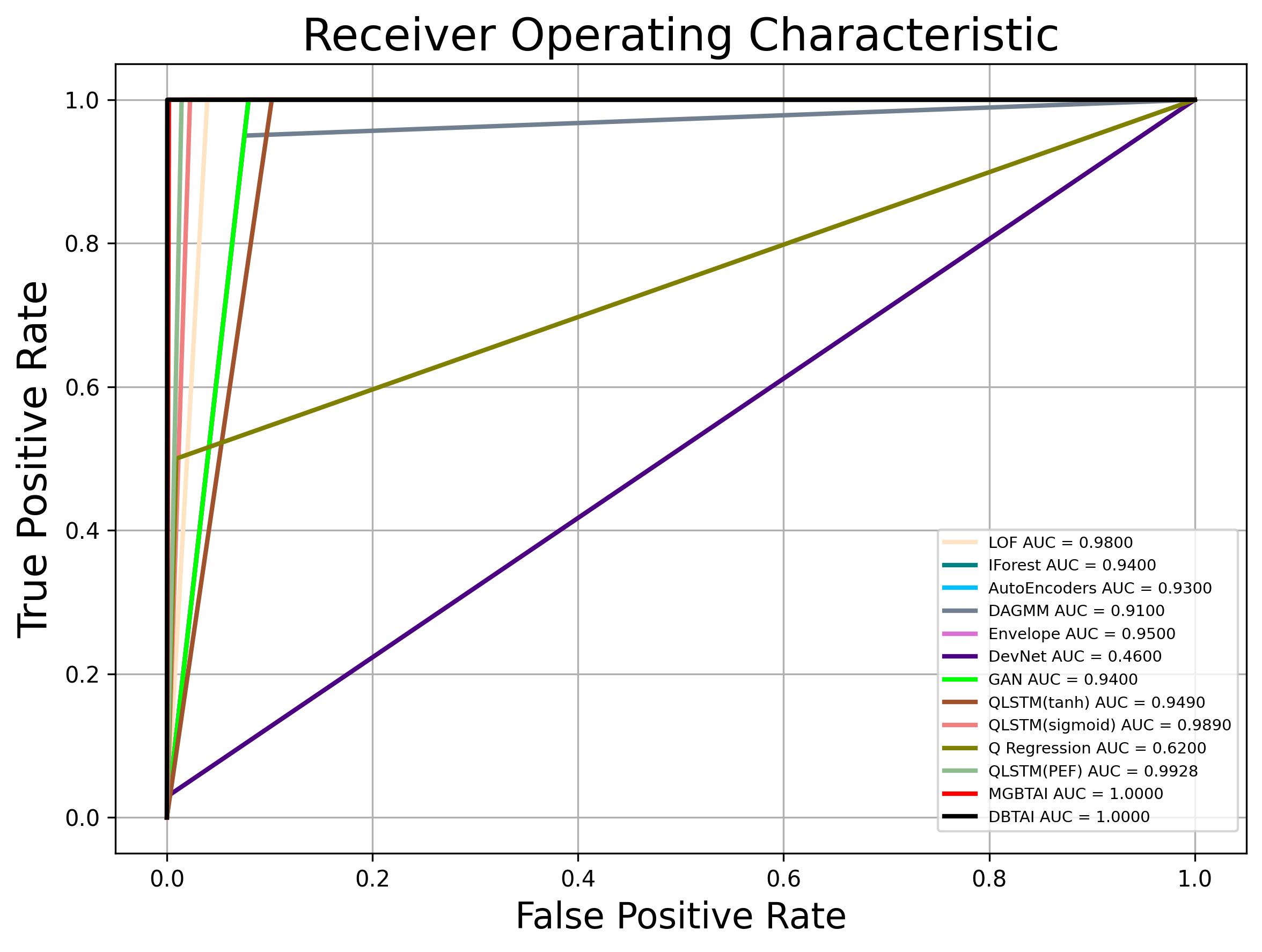
(f) Speed$\_$t4013

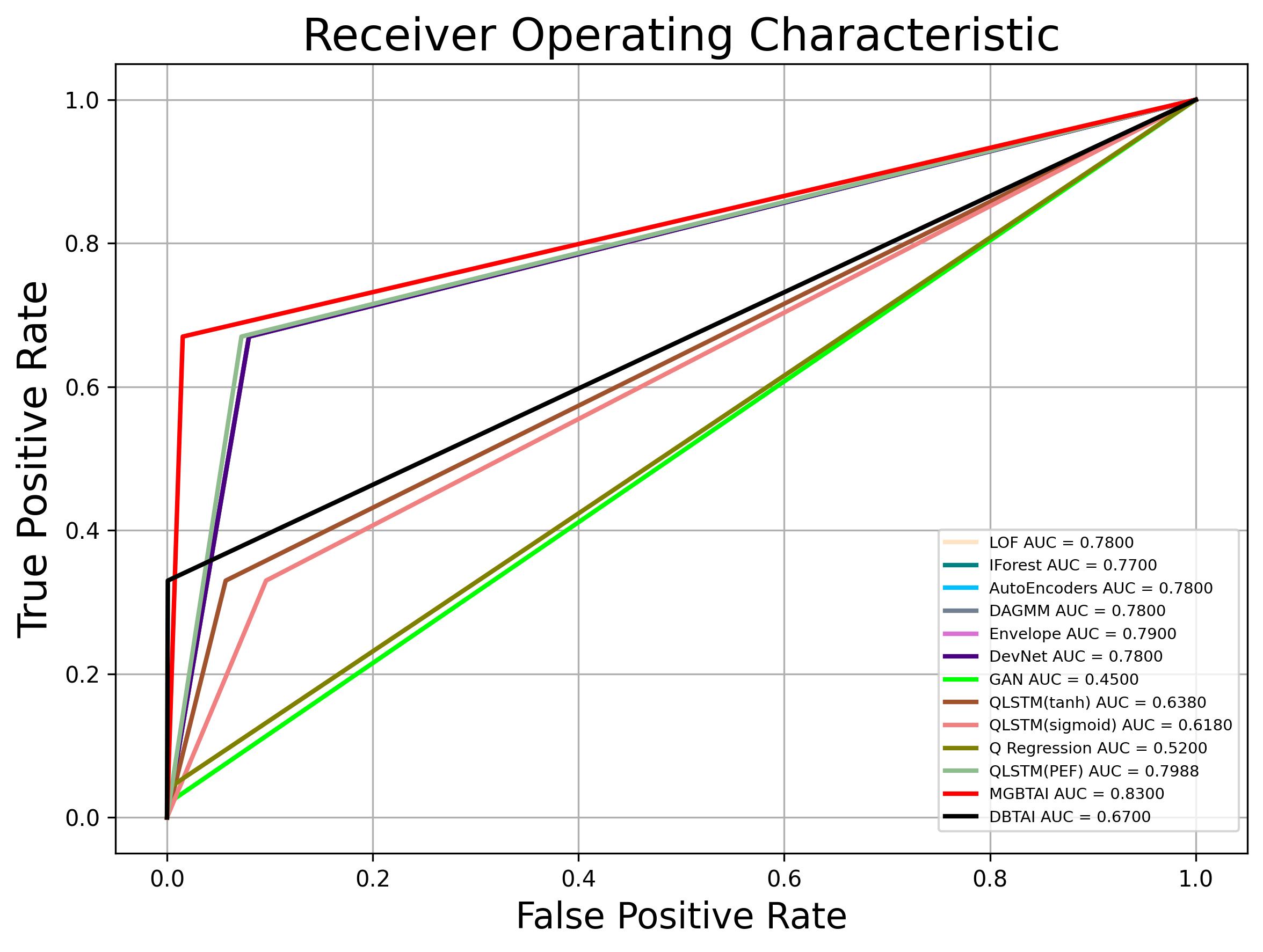
(a) TravelTime$\_$387

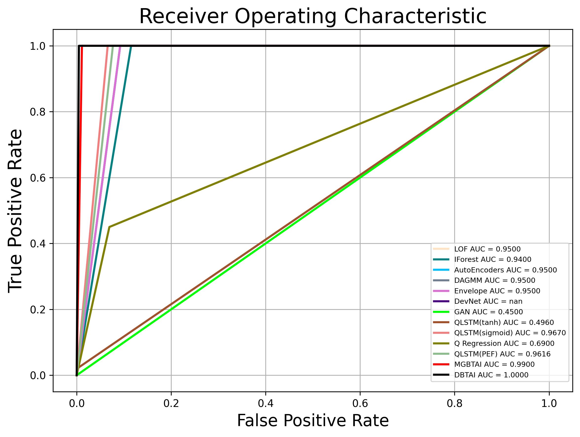
(b) TravelTime$\_$451

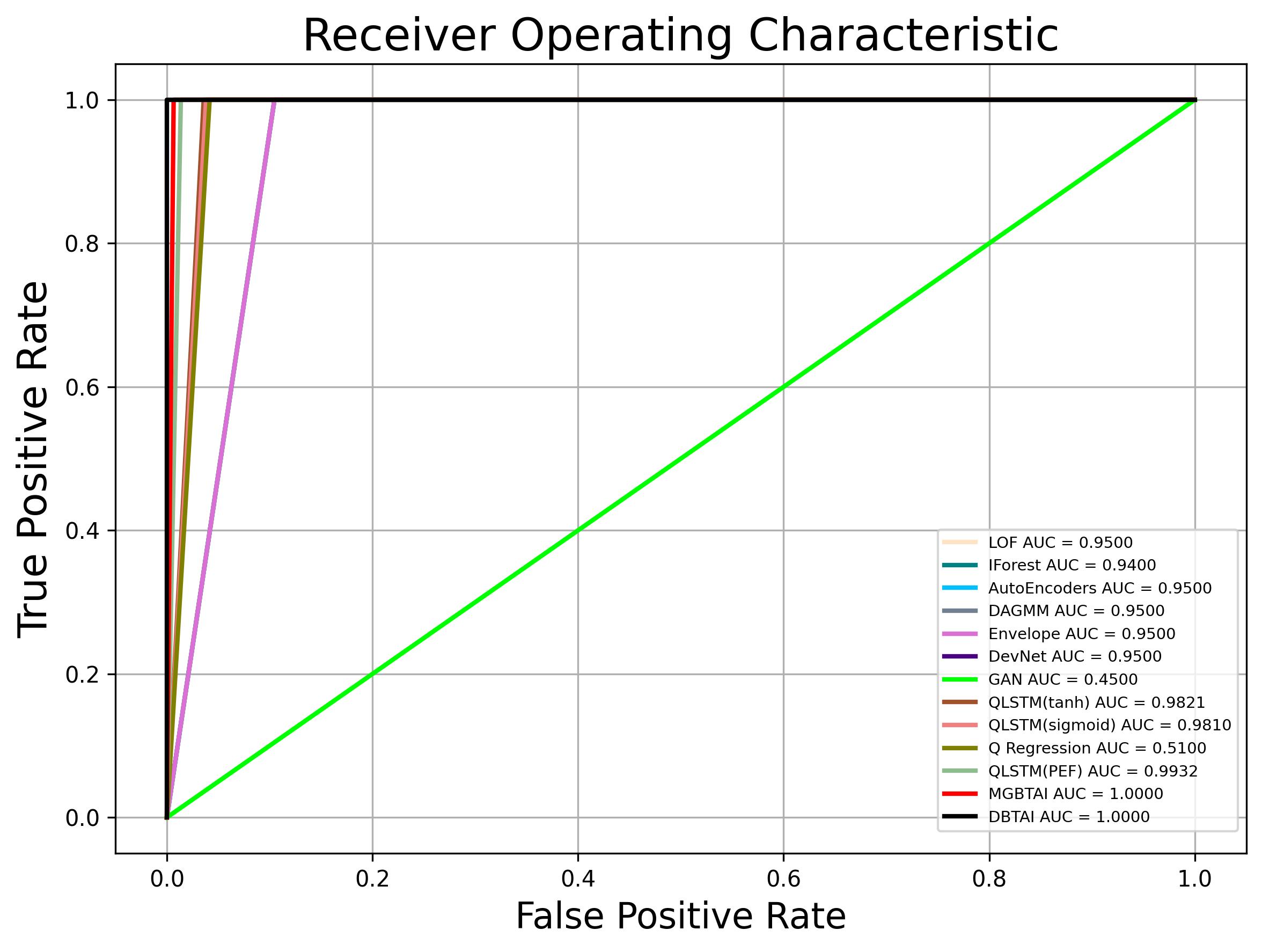
(c) Occupancy$\_$6005

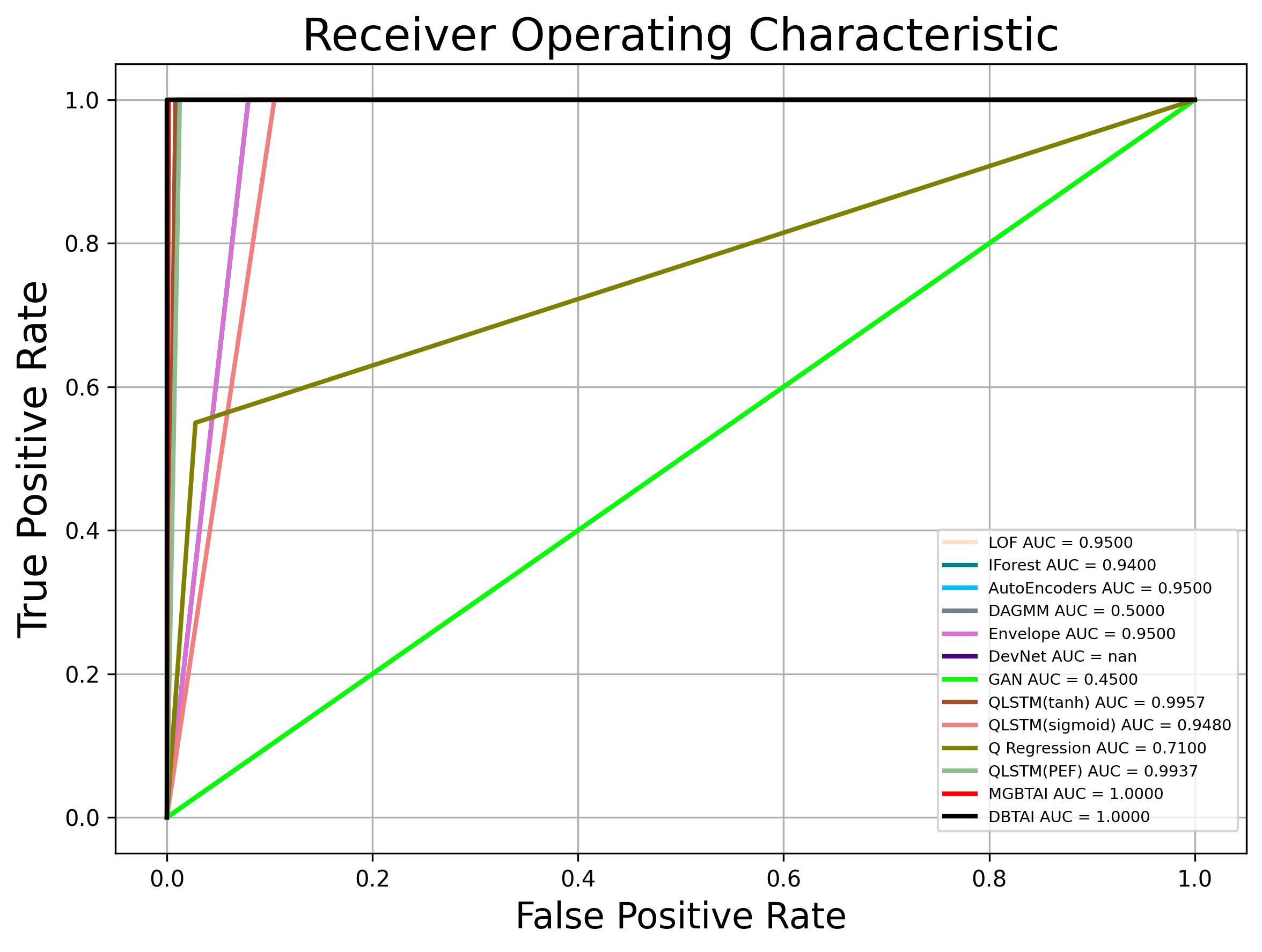
(d) Occupancy$\_$t4013

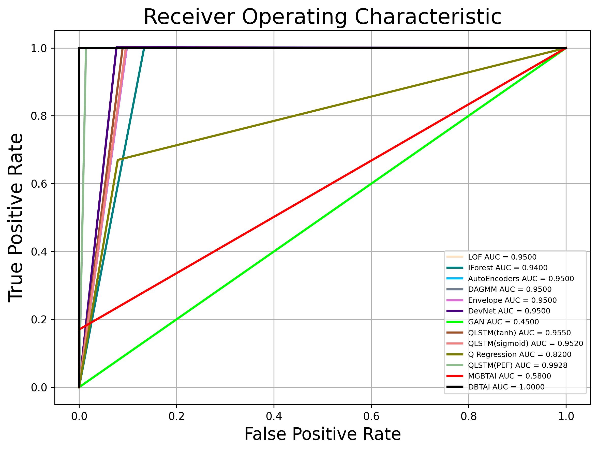
(e) yahoo$\_$syn1

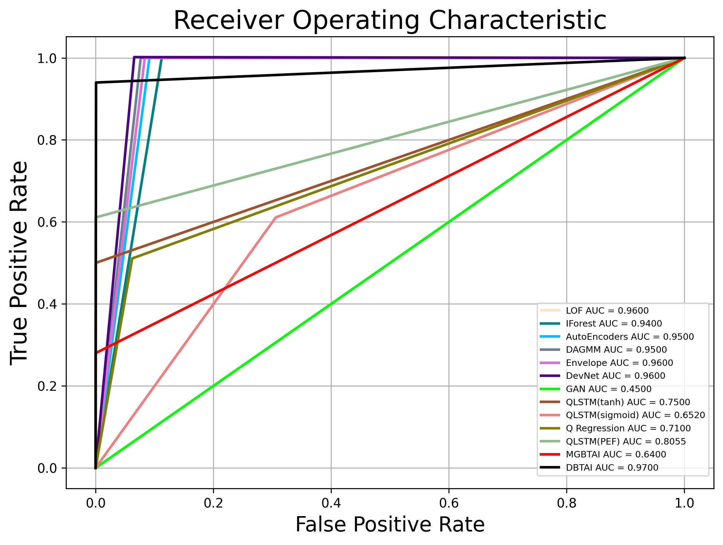
(f) yahoo$\_$syn2

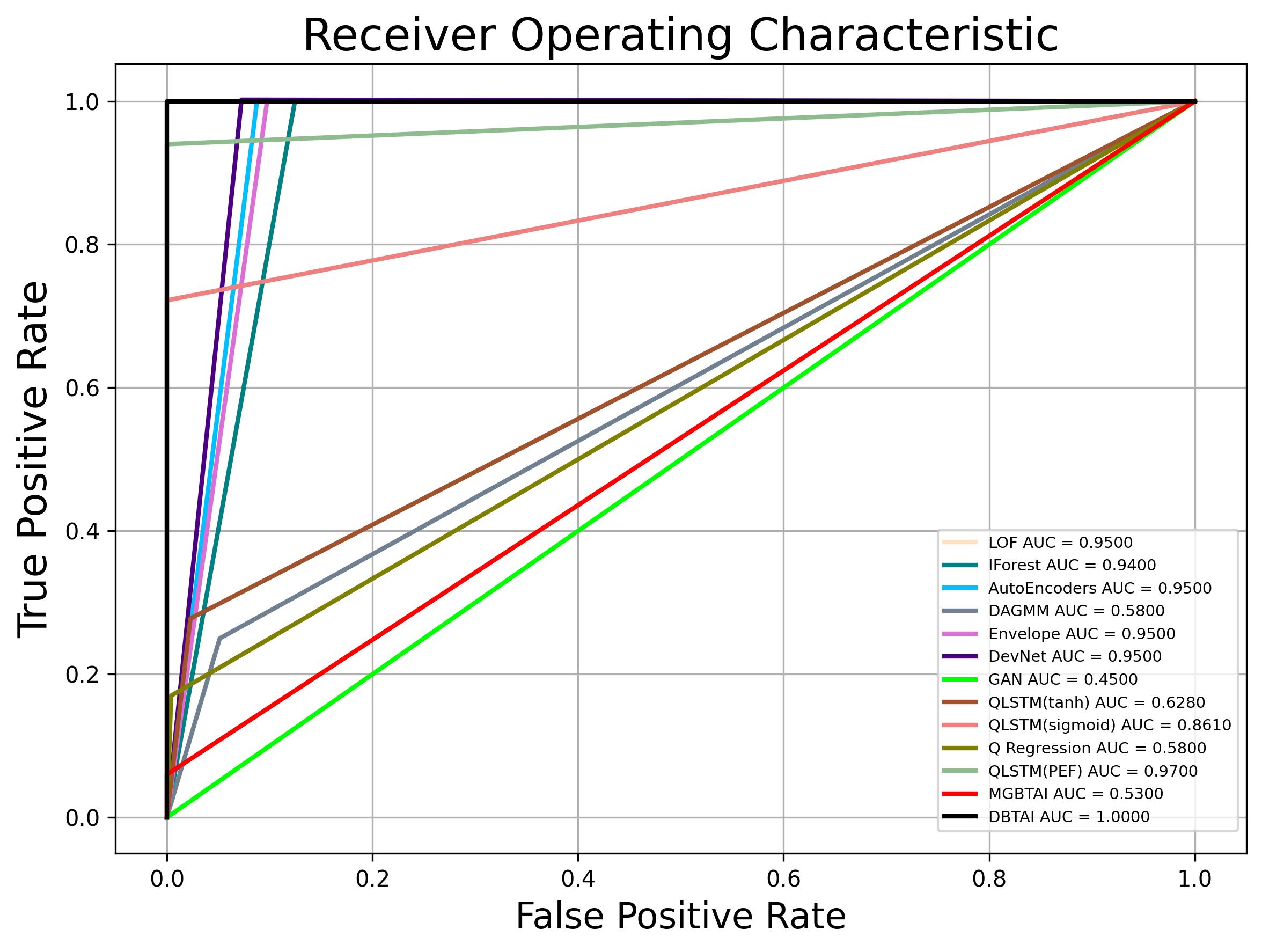
(a) yahoo$\_$syn9

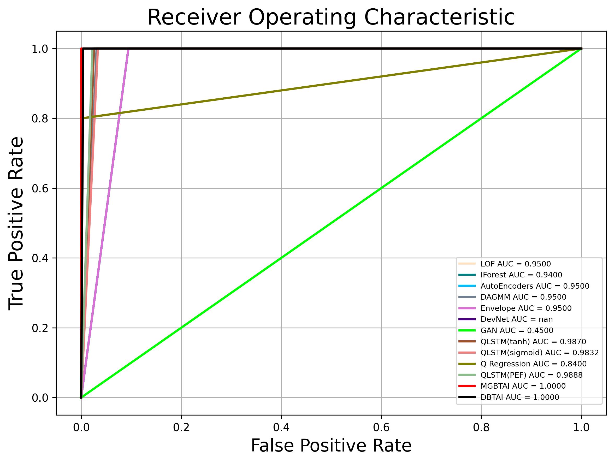
(b) aws1

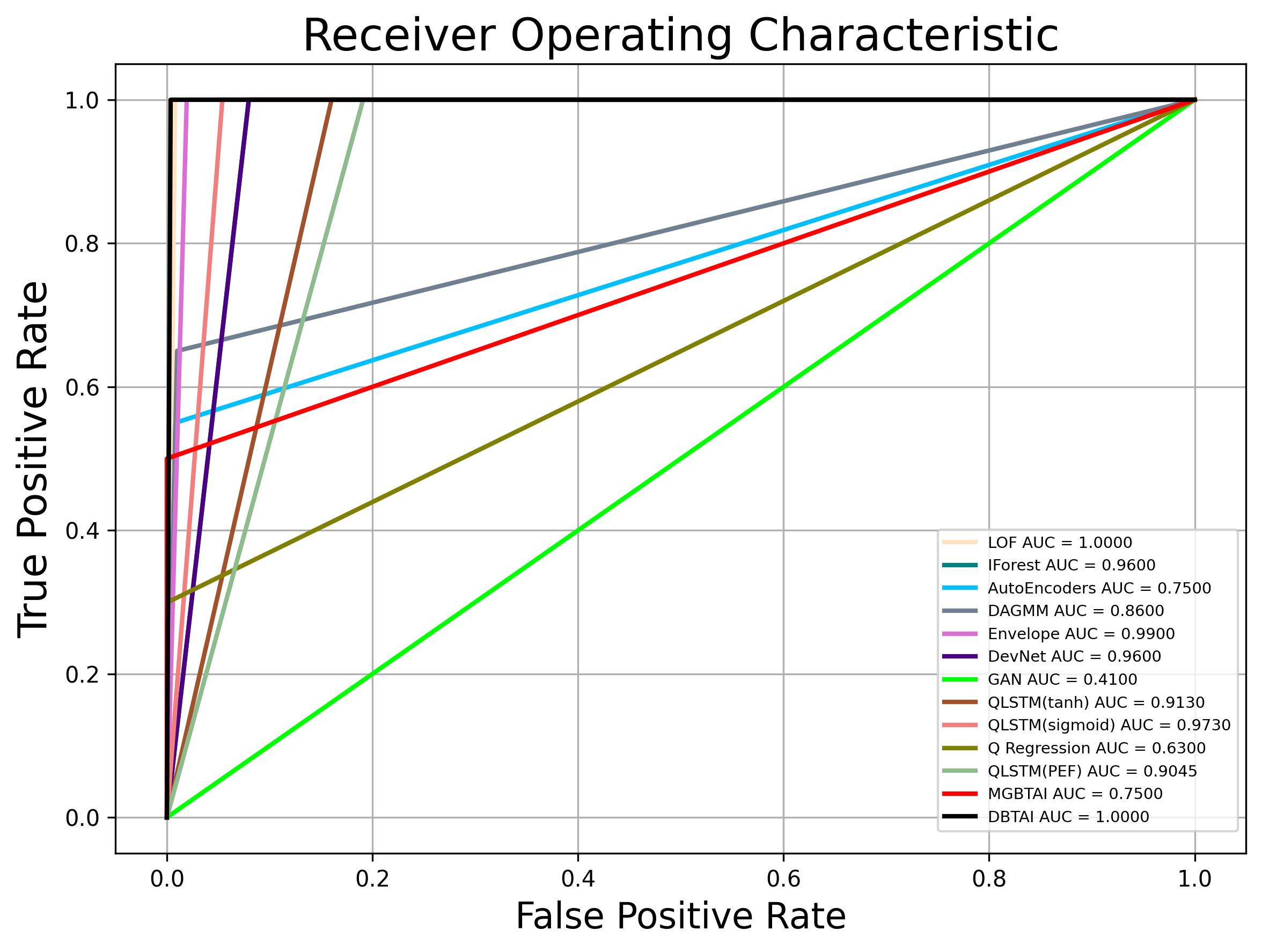
(c) aws2

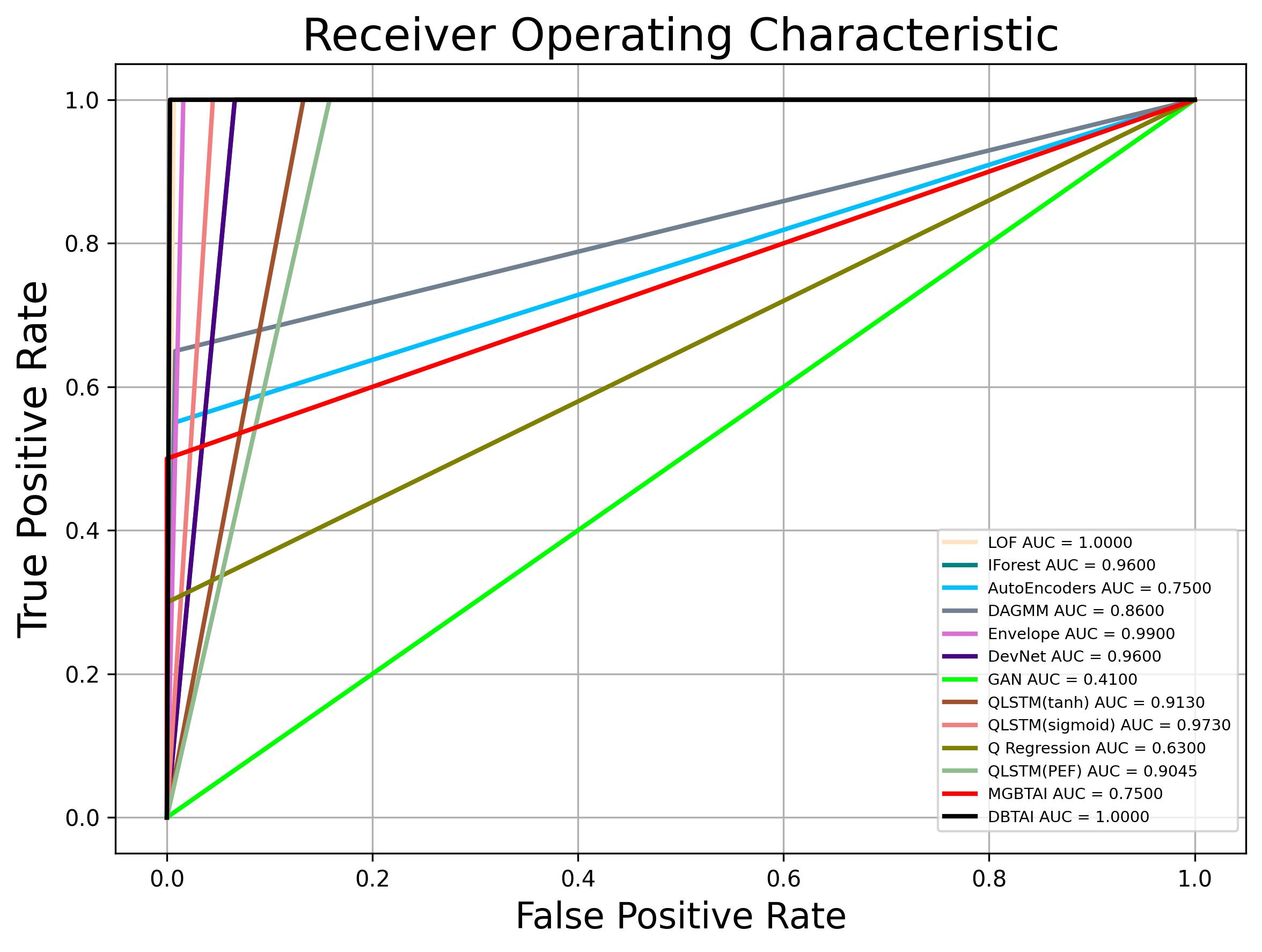
(d) aws3

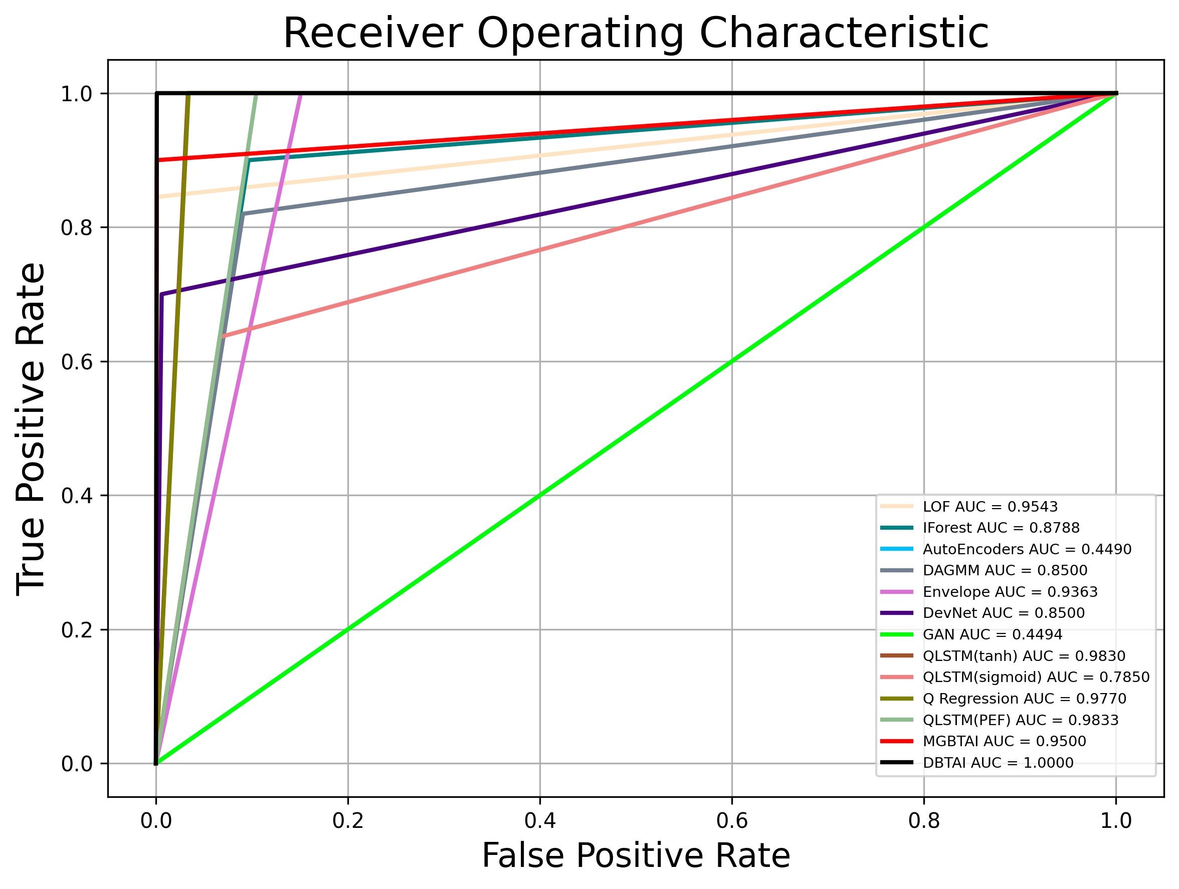
(e) aws$\_$syn1

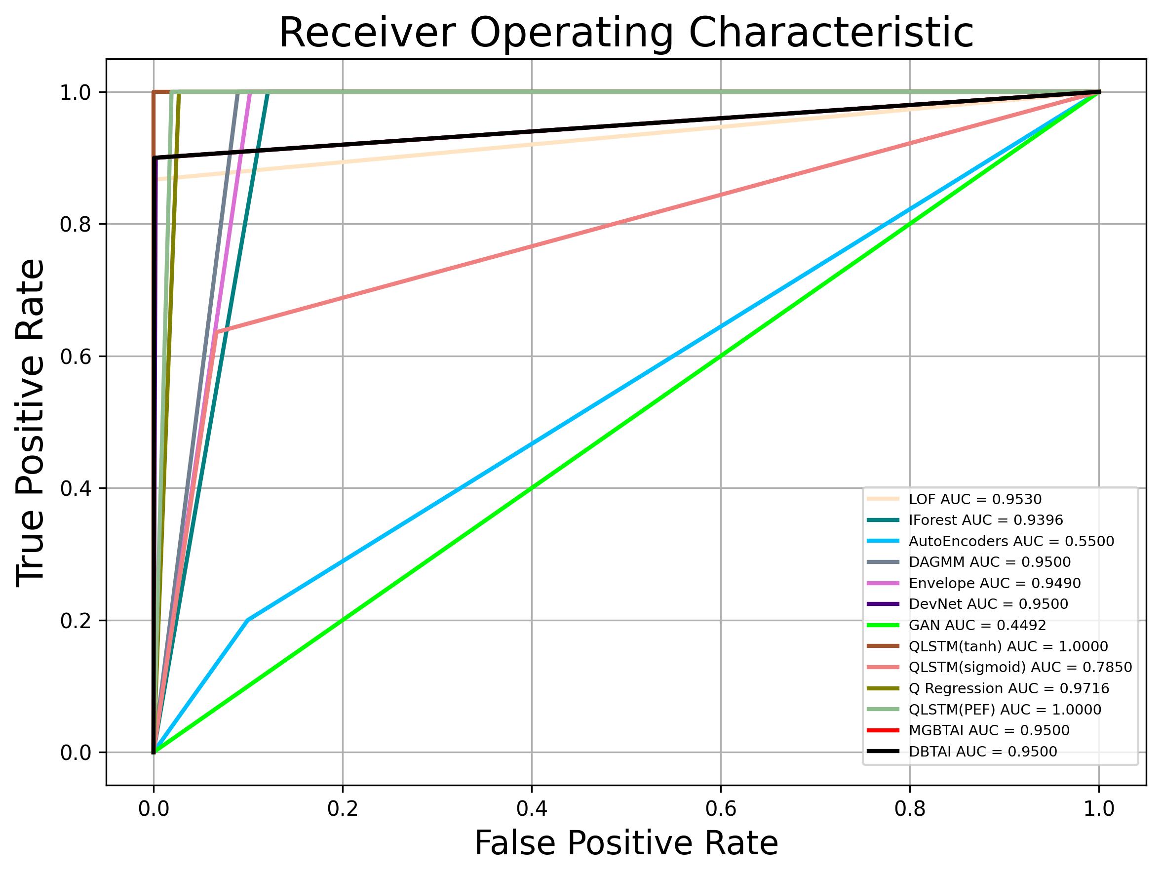
(f) aws$\_$syn3

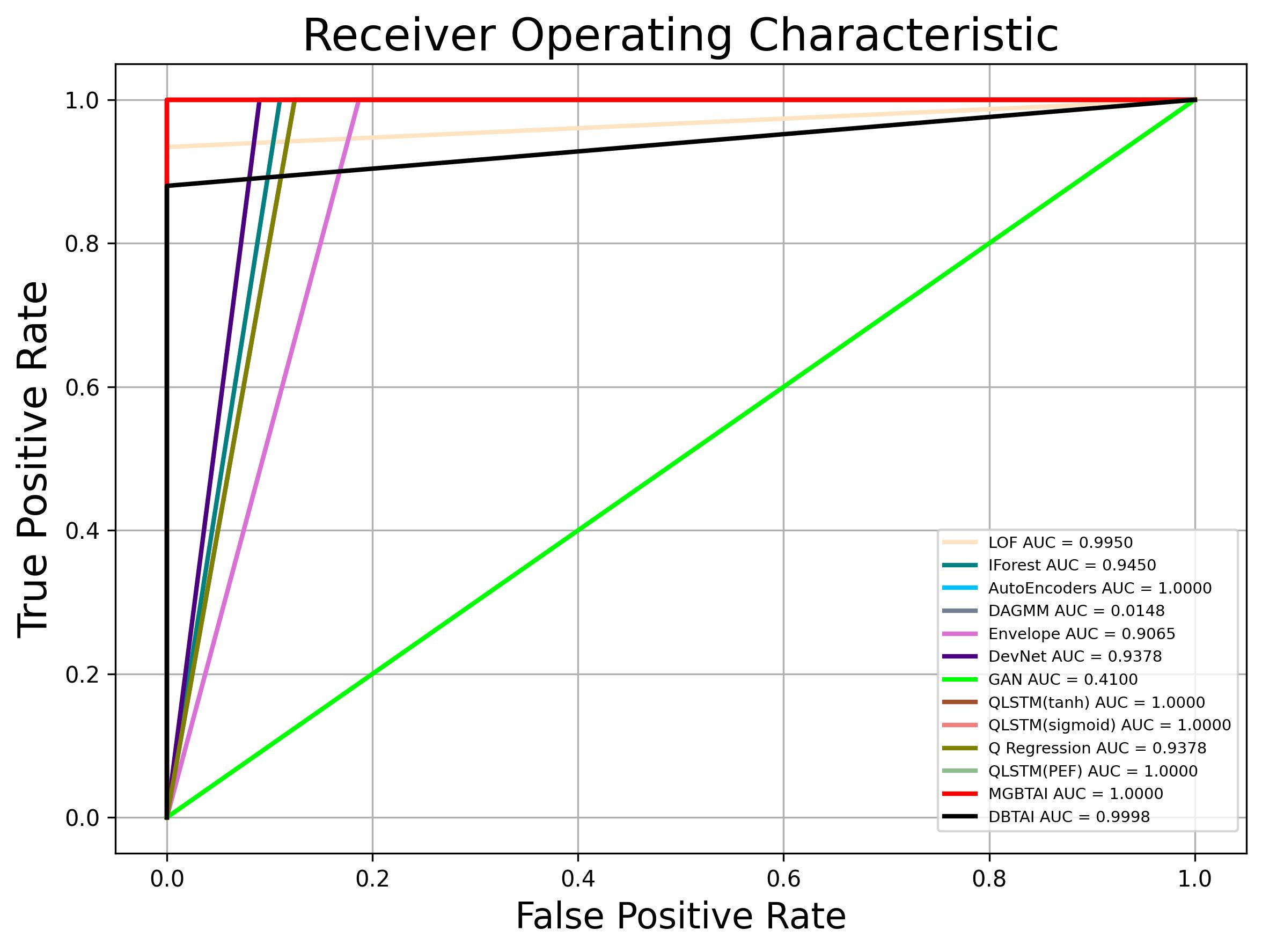
(a) Industrial$\_$2

Figure 10: AUC ROC comparison of Tree Based Approaches with other SOTA baselines for univariate data

References

- [1] M. Antunes, D. Gomes, and R. L. Aguiar. Knee/elbow estimation based on first derivative threshold. In IEEE Fourth International Conference on Big Data Computing Service and Applications (BigDataService), pages 237–240, 2018.
- [2] T. R. Bandaragoda et al. Isolation-based anomaly detection using nearest-neighbor ensembles. Computational Intelligence, 34(4):968–998, November 2018.
- [3] L. Breiman. Random forests. Machine learning, 45:5–32, 2001.
- [4] M. M. Breunig et al. LOF: identifying density-based local outliers. ACM SIGMOD Record, 29(2):93–104, June 2000.
- [5] G. O. Campos et al. On the evaluation of unsupervised outlier detection: measures, datasets, and an empirical study. Data Mining and Knowledge Discovery, 30(4):891–927, July 2016.
- [6] Will Cappelli. Gartner, Inc. https://www.gartner.com/en/documents/3342317, 2016. [Online; last accessed 16-January-2024].
- [7] A. Castellani, S. Schmitt, and S. Squartini. Real-World Anomaly Detection by Using Digital Twin Systems and Weakly Supervised Learning. IEEE Transactions on Industrial Informatics, 17(7):4733–4742, July 2021.
- [8] R. Chalapathy and S. Chawla. Deep Learning for Anomaly Detection: A Survey. 2019.
- [9] V. Chandola, A. Banerjee, and V. Kumar. Anomaly detection: A survey. ACM Computing Surveys, 41(3):1–58, July 2009.
- [10] F. Chollet et al. Keras. https://keras.io, 2015.
- [11] A. A. Cook, G. Misirli, and Z. Fan. Anomaly Detection for IoT Time-Series Data: A Survey. IEEE Internet of Things Journal, 7(7):6481–6494, July 2020.
- [12] Y. Cui, Z. Liu, and S. Lian. A Survey on Unsupervised Anomaly Detection Algorithms for Industrial Images. IEEE Access, 11:55297–55315, 2023.
- [13] A. Deng and B. Hooi. Graph Neural Network-Based Anomaly Detection in Multivariate Time Series. In Proceedings of the AAAI conference on artificial intelligence, volume 35, pages 4027–4035, June 2021. arXiv:2106.06947 [cs].
- [14] Y. Djenouri et al. A Survey on Urban Traffic Anomalies Detection Algorithms. IEEE Access, 7:12192–12205, 2019.
- [15] R. Domingues et al. A comparative evaluation of outlier detection algorithms: Experiments and analyses. Pattern Recognition, 74:406–421, February 2018.
- [16] K. Doshi, S. Abudalou, and Y. Yilmaz. Reward Once, Penalize Once: Rectifying Time Series Anomaly Detection. Proceedings of International Joint Conference on Neural Networks, July 2022.
- [17] S. Eltanbouly et al. Machine Learning Techniques for Network Anomaly Detection: A Survey. In IEEE International Conference on Informatics, IoT, and Enabling Technologies (ICIoT), pages 156–162. IEEE, February 2020.
- [18] S. M. Erfani et al. High-dimensional and large-scale anomaly detection using a linear one-class SVM with deep learning. Pattern Recognition, 58:121–134, October 2016.
- [19] F. Falcão et al. Quantitative comparison of unsupervised anomaly detection algorithms for intrusion detection. In Proceedings of the 34th ACM/SIGAPP Symposium on Applied Computing, pages 318–327. ACM, April 2019.
- [20] D. Fourure et al. Anomaly Detection: How to Artificially Increase Your F1-Score with a Biased Evaluation Protocol. In Machine Learning and Knowledge Discovery in Databases. Applied Data Science Track, volume 12978, pages 3–18. Springer International Publishing, 2021.
- [21] A. K. Ghosh and A. Schwartzbard. A Study in Using Neural Networks for Anomaly and Misuse Detection. 1999.
- [22] N. Goix. How to Evaluate the Quality of Unsupervised Anomaly Detection Algorithms? arXiv preprint arXiv:1607.01152, 2016.
- [23] I. Goodfellow et al. Generative adversarial networks. Communications of the ACM, 63(11):139–144, 2020.
- [24] R. A. A. Habeeb et al. Real-time big data processing for anomaly detection: A Survey. International Journal of Information Management, 45:289–307, April 2019.
- [25] S. Han et al. Adbench: Anomaly detection benchmark. Advances in Neural Information Processing Systems, 35:32142–32159, 2022.
- [26] K. Heller et al. One Class Support Vector Machines for Detecting Anomalous Windows Registry Accesses. 2003.
- [27] S. Hochreiter and J. Schmidhuber. Long Short-Term Memory. Neural Computation, 9(8):1735–1780, November 1997.
- [28] A. Huet, J. M. Navarro, and D. Rossi. Local Evaluation of Time Series Anomaly Detection Algorithms. In Proceedings of the 28th ACM SIGKDD Conference on Knowledge Discovery and Data Mining, pages 635–645. ACM, August 2022.
- [29] V. Jacob et al. Exathlon: a benchmark for explainable anomaly detection over time series. Proceedings of the VLDB Endowment, 14(11):2613–2626, July 2021.
- [30] S. Kim et al. Towards a Rigorous Evaluation of Time-Series Anomaly Detection. Proceedings of the AAAI Conference on Artificial Intelligence, 36(7):7194–7201, June 2022.
- [31] B. Kiran, D. Thomas, and R. Parakkal. An Overview of Deep Learning Based Methods for Unsupervised and Semi-Supervised Anomaly Detection in Videos. Journal of Imaging, 4(2):36, February 2018.
- [32] T. M. Kodinariya and P. R. Makwana. Review on determining number of cluster in k-means clustering. International Journal, 1(6):90–95, 2013.
- [33] SB Kotsiantis. Supervised Machine Learning: A Review of Classification Techniques. Informatica, 31:249–268, 2007.
- [34] F. T. Liu, K. M. Ting, and Z. H. Zhou. Isolation forest. In eighth ieee international conference on data mining, pages 413–422. IEEE, 2008.
- [35] J. Liu et al. Deep Industrial Image Anomaly Detection: A Survey. ArXiV-2301, 2023.
- [36] T. Lu, L. Wang, and X. Zhao. Review of Anomaly Detection Algorithms for Data Streams. Applied Sciences, 13(10):6353, May 2023.
- [37] T. Luo and S. G. Nagarajan. Distributed Anomaly Detection Using Autoencoder Neural Networks in WSN for IoT. In IEEE International Conference on Communications (ICC), pages 1–6, May 2018. ISSN: 1938-1883.
- [38] A. P. Mathur and N. O. Tippenhauer. SWaT: a water treatment testbed for research and training on ICS security. In International Workshop on Cyber-physical Systems for Smart Water Networks (CySWater), pages 31–36. IEEE, April 2016.
- [39] G. Pang et al. Deep Learning for Anomaly Detection: A Review. ACM Computing Surveys, 54(2):1–38, March 2022.
- [40] J. Paparrizos et al. TSB-UAD: an end-to-end benchmark suite for univariate time-series anomaly detection. Proceedings of the VLDB Endowment, 15(8):1697–1711, April 2022.
- [41] F. Pedregosa et al. Scikit-learn: Machine Learning in Python. Journal of Machine Learning Research, 12(85):2825–2830, 2011.
- [42] P. J. Rousseeuw and K. V. Driessen. A Fast Algorithm for the Minimum Covariance Determinant Estimator. Technometrics, 41(3):212–223, August 1999.
- [43] S. Saha et al. Quantile LSTM: A Robust LSTM for Anomaly Detection In Time Series Data. IEEE Transactions on Artificial Intelligence, January 2024.
- [44] D. Samariya and A. Thakkar. A Comprehensive Survey of Anomaly Detection Algorithms. Annals of Data Science, 10(3):829–850, June 2023.
- [45] J. Sarkar, S. Saha, and S. Sarkar. Efficient anomaly identification in temporal and non-temporal industrial data using tree based approaches. Applied Intelligence, 53(8):8562–8595, April 2023.
- [46] J. Sarkar et al. d-BTAI: The Dynamic-Binary Tree Based Anomaly Identification Algorithm for Industrial Systems. In Advances and Trends in Artificial Intelligence. From Theory to Practice, Lecture Notes in Computer Science, pages 519–532. Springer International Publishing, 2021.
- [47] S. Schmidl, P. Wenig, and T. Papenbrock. Anomaly detection in time series: a comprehensive evaluation. Proceedings of the VLDB Endowment, 15(9):1779–1797, May 2022.
- [48] G. Steinbuss and K. Böhm. Benchmarking Unsupervised Outlier Detection with Realistic Synthetic Data. ACM Transactions on Knowledge Discovery from Data, 15(4):1–20, August 2021.
- [49] A. I. Tambuwal and D. Neagu. Deep Quantile Regression for Unsupervised Anomaly Detection in Time-Series. SN Computer Science, 2(6):475, November 2021.
- [50] James Verbus. Linkedin Engineering. https://engineering.linkedin.com/blog/2019/isolation-forest, 2019. [Online; last accessed 16-January-2024].
- [51] S. Wang et al. Machine Learning in Network Anomaly Detection: A Survey. IEEE Access, 9:152379–152396, 2021.
- [52] P. Wenig, S. Schmidl, and T. Papenbrock. TimeEval: a benchmarking toolkit for time series anomaly detection algorithms. Proceedings of the VLDB Endowment, 15(12):3678–3681, August 2022.
- [53] R. Wu and E. J. Keogh. Current Time Series Anomaly Detection Benchmarks are Flawed and are Creating the Illusion of Progress (Extended Abstract). In IEEE 38th International Conference on Data Engineering (ICDE), pages 1479–1480. IEEE, May 2022.
- [54] H. Xu et al. Deep Isolation Forest for Anomaly Detection. IEEE Transactions on Knowledge and Data Engineering, 35(12):12591–12604, December 2023.
- [55] C. Yin et al. Anomaly Detection Based on Convolutional Recurrent Autoencoder for IoT Time Series. IEEE Transactions on Systems, Man, and Cybernetics: Systems, 52(1):112–122, January 2022.
- [56] Y. Zhang et al. Statistics-based outlier detection for wireless sensor networks. International Journal of Geographical Information Science, 26(8):1373–1392, August 2012.
- [57] Y. Zhao, Z. Nasrullah, and Z. Li. PyOD: A Python Toolbox for Scalable Outlier Detection. Journal of Machine Learning Research, 20(96):1–7, 2019.
- [58] B. Zong et al. Deep Autoencoding Gaussian Mixture Model for Unsupervised Anomaly Detection. February 2018.