Constant mean curvature graphs with prescribed asymptotic values in $\mathbb{E}(-1,\tau)$

Abstract.

In the homogeneous manifold $\mathbb{E}(-1,\tau),$ for $0<H<\tfrac{1}{2},$ we prove the existence of entire $H$-graphs which are asymptotic to a rectifiable curve of the asymptotic boundary. We also find necessary and sufficient conditions for the existence of $H$-graphs over unbounded domains having prescribed, possibly infinite boundary data.

1. Introduction

Constant mean curvature surfaces in simply connected homogeneous 3-manifolds have been a subject of extensive research by various authors over the past two decades. In particular, considerable attention has been devoted to 3-manifolds with an isometry group of dimension at least 4. These 3-manifolds, excluding the hyperbolic space $\mathbb{H}^{3}$, can be classified in a 2-parameter family denoted as $\mathbb{E}(\kappa,\tau)$, where $\kappa$ and $\tau$ are real numbers. This classification depends on the property of the $\mathbb{E}(\kappa,\tau)$-spaces to admit a Riemannian submersion $\pi\colon\mathbb{E}(\kappa,\tau)\to\mathbb{M}(\kappa)$ over the complete simply connected Riemannian surface with constant curvature $\kappa$ whose fibers are the integral curves of the unique unitary Killing vector field $\xi\in\mathfrak{X}(\mathbb{E})$ such that $\tau$ is the bundle curvature (that is $\nabla_{X}\xi=\tau X\wedge\xi$ for all vector fields $X\in\mathfrak{X}(\mathbb{E}),$ where $\nabla$ is the Levi-Civita connection of $\mathbb{E}$ and $\wedge$ is the cross product in $\mathbb{E}$ with respect to a chosen orientation, see [11]).

This geometric setup naturally prompts the question of investigating graphs, i.e. sections of the Riemannian submersion obtained deforming a fixed zero section through the flow lines, with constant mean curvature over specific domains of $\mathbb{M}(\kappa)$. Such an approach can be considered as a non-parametric version of the constant mean curvature condition (see Section 4).

In this paper we focus on the case $\kappa=-1$ and investigate graphs with constant mean curvature $H$ that will be referred as an $H$-graphs or, whenever $H$ is not desired to be explicit, CMC graphs.

One of the pioneering works in this setting is due to Nelli and Rosenberg in $\mathbb{H}^{2}\times\mathbb{R}=\mathbb{E}(-1,0)$ (see [16]), who solved the following problems.

• The existence of a unique entire minimal graph with arbitrarily prescribed asymptotic values.

• The Jenkins–Serrin problem over relatively compact domains, that is, to find necessary and sufficient conditions that guarantee the existence and uniqueness of a solution for the Dirichlet problem for the minimal surface equation with possibly infinite boundary data.

So far, no result with an analogous statement as in [16] has been given about CMC graphs having prescribed asymptotic boundary value. In the classical model, i.e. the one where the zero section is the minimal surface invariant by rotation (see Section 2), such a result cannot be achieved due to the Slab Theorem (see [8]), which implies that any entire function satisfying the constant mean curvature equation must diverges. The aim of this paper is to show that, if we assume the zero section to have constant mean curvature $H$, it is possible to prove a statement analogous to the one of Nelli and Rosenberg [16] about the existence of entire $H$-graphs in $\mathbb{E}(-1,\tau)$.

In particular, for any rectifiable curve $\Gamma$ in $\partial_{\infty}\mathbb{E}(-1,\tau)=\pi^{-1}(\partial_{\infty}\mathbb{H}^{2})$ that is the graph of a function of $\partial_{\infty}\mathbb{H}^{2}$, we construct an entire graph $\Sigma$ of subcritical constant mean curvature $H$ that is asymptotic to $\Gamma$. This can be done by changing the model of $\mathbb{E}(-1,\tau)$ so that the plane $\left\{z=0\right\}$ has constant mean curvature $0<H<1/2$. In such a way, we have a direct control over the symmetries of the graph $\Sigma$. Indeed, by means of the Maximum Principle one can prove that $\Sigma$ inherits the symmetries of the curve $\Gamma$. We cannot cover the case $H=1/2$ because of the half-space property given in [18, 12]. Moreover, due to our result, a half-space theorem for entire $H$-graphs with $H<1/2$ cannot be proven.

Concerning the Jenkins–Serrin problem, several extensions have been achieved. A Jenkins–Serrin problem for CMC graphs in $\mathbb{H}^{2}\times\mathbb{R}$ over relatively compact domains of $\mathbb{H}^{2}$ was proved by Hauswirth, Rosenberg and Spruck in [9] and by Eichmair and Metger in [5] in a general product space $M\times\mathbb{R}$. Furthermore, in [4], the author, together with Manzano and Nelli, proves an analogous result for minimal graphs in a general Killing submersion, which include the space $\mathbb{E}(-1,\tau).$ In [13] Mazet, Rodriguez and Rosenberg proved in $\mathbb{H}^{2}\times\mathbb{R}$ a Jenkins–Serrin type result for minimal surfaces over unbounded domains of $\mathbb{H}^{2}$, allowing the asymptotic boundary of such domains to contain open subsets of $\partial_{\infty}\mathbb{H}^{2}$. Later, Melo proved the same result in the space $\mathbb{E}(-1,\tau)$ [15]. A result for $H$-graphs in $\mathbb{H}^{2}\times\mathbb{R}$, similar to [13], was proved by Folha and Melo in [6]. They solved the Jenkins–Serrin problem for $H$-graphs with $0<H<1/2$ over an unbounded domain whose asymptotic boundary does not contain open subsets of $\partial_{\infty}\mathbb{H}^{2}$. We use the constructed barriers to extend the results in [6, 15], showing that in the model we consider we are able to solve the Jenkins–Serrin problem over a larger family of unbounded domains $\Omega$ of $\mathbb{H}^{2}$. In particular, we solve the following Dirichlet problem:

$$\begin{cases}H(u)=H&\textrm{ in }D,\\ u=f_{i}&\textrm{ on }C_{i},\\ u=+\infty&\textrm{ on }A_{i},\\ u=-\infty&\textrm{ on }B_{i},\\ u=F&\textrm{ on }\Gamma,\end{cases}$$

where $A_{i},\,B_{i},\,C_{i}$ are such that

$$A_{i}\cup B_{i}\cup C_{i}=\partial\Omega,\quad\kappa_{g}(A_{i})=2H,\quad\kappa_{g}(B_{i})=-2H\quad\textrm{and}\quad\kappa_{g}(C_{i})\geq 2H,$$

$\Gamma$ is the asymptotic boundary of $D$, that is $\Gamma\subset\partial_{\infty}\mathbb{H}^{2}$, and $f_{i}\in\mathcal{C}^{\infty}(C_{i})$ and $F\in\mathcal{C}^{\infty}(\Gamma)$.

The paper is organized as follows. Section 2 is a description of the basic properties of the space $\mathbb{E}(-1,\tau)$. In Section 3 we recall the constant mean curvature graphs that are invariant with respect to a one-parameter group of isometries of $\mathbb{E}(-1,\tau)$ studied by Peñafiel in [19] and we study their asymptotic behaviour. In Section 4 we introduce the new model for $\mathbb{E}(-1,\tau)$ in which the plane $\left\{z=0\right\}$ has constant mean curvature $H\in(0,1/2)$. In Section 5, we use the surfaces studied in Section 3 to construct barriers for the Dirichlet Problem for the constant mean curvature equation. Finally, the main results of this paper are given in Sections 6 and 7, where, respectively, we prove the existence of entire $H$-graphs with prescribed asymptotic boundary and the Jenkins–Serrin problem.

2. The space $\mathbb{E}(-1,\tau)$

The space $\mathbb{E}(-1,\tau)$ is the homogeneous 3-dimensional manifold defined as $\Omega\times\mathbb{R}$, endowed with the metric

$$ds^{2}_{\lambda}=\lambda^{2}\left(dx^{2}+dy^{2}\right)+\left[dt-2\tau\lambda\left(\left(\tfrac{1}{\lambda}\right)_{y}dx-\left(\tfrac{1}{\lambda}\right)_{x}dy\right)\right]^{2}.$$ (2.1)

where $\Omega=\left\{(x,y)\in\mathbb{R}^{2}\mid\lambda(x,y)>0\right\}$ and $\lambda\in\mathcal{C}^{\infty}(\Omega)$ satisfies $\Delta(\log(\lambda))-\lambda^{2}=0$.

Notice that $\left(\Omega,\lambda^{2}(dx^{2}+dy^{2})\right)$ is isometric to the hyperbolic plane $\mathbb{H}^{2}$ with a constant sectional curvature of $-1$ and the Killing submersion is $\pi(x,y,t)=(x,y)$ with $\partial_{t}$ being the unitary Killing field satisfying the identity $\nabla_{X}\partial_{t}=\tau X\wedge\partial_{t}$ for any $X\in\mathfrak{X}(\mathbb{E})$. In this context, we call vertical every vector field parallel to $\partial_{t},$ and horizontal every vector field orthogonal to $\partial_{t}$. In this model, the mean curvature of the graph $\Sigma_{u}=(x,y,u(x,y))\subset\Omega\times\mathbb{R}$ of the function $u\in\mathcal{C}^{2}(\Omega)$ is given in the divergent form as

$$2H=\mathop{\rm div}\nolimits\left(\frac{Gu}{\sqrt{1+\|Gu\|^{2}}}\right),$$ (2.2)

where $\mathop{\rm div}\nolimits(\cdot)$ and $\|\cdot\|$ are the divergence and norm of $\mathbb{H}^{2}$ in the conformal metric $\lambda^{2}(dx^{2}+dy^{2}),$ and $Gu=\left(u_{x}-\tfrac{2\tau\lambda_{y}}{\lambda}\right)\frac{\partial_{x}}{\lambda^{2}}+\left(u_{y}+\tfrac{2\tau\lambda_{x}}{\lambda}\right)\frac{\partial_{y}}{\lambda^{2}}$ is the generalized gradient.

Depending on the choice of $\lambda,$ we have two classical models to describe $\mathbb{E}(-1,\tau):$

• If $\lambda(x,y)=\lambda_{\mathcal{H}}(x,y)=\frac{1}{y}$, we get the half-plane model for $\mathbb{H}^{2}$ and the half-space model $\mathcal{H}$ for $\mathbb{E}(-1,\tau),$ where the vertical boundary is $(\left\{y=0\right\}\cup\left\{\infty\right\})\times\mathbb{R}\equiv(\mathbb{R}\cup\left\{\infty\right\})\times\mathbb{R}.$

• If $\lambda(x,y)=\lambda_{\mathcal{C}}(x,y)=\frac{2}{1-x^{2}-y^{2}}$, we obtain the Poincaré Disk model for $\mathbb{H}^{2}$ and the cylindrical model $\mathcal{C}$ for $\mathbb{E}(-1,\tau),$ with $\mathbb{S}(1)\times\mathbb{R}$ as vertical boundary.

Using the complex coordinate $z=x+iy$, the isometries between this two models are given by lifting the Möbius transformation of $\mathbb{H}^{2}$ (see [1] for more details):

$$\begin{array}[]{rccc}\psi\colon&\overline{\mathcal{H}}&\to&\overline{\mathcal{C}}\\ &(x,y,t)&\mapsto&\left(\frac{z-i}{z+1},t-4\tau\arctan\left(\frac{x}{y+1}\right)\right),\end{array}$$

and

$$\begin{array}[]{rccc}\psi^{-1}\colon&\overline{\mathcal{C}}&\to&\overline{\mathcal{H}}\\ &(x,y,t)&\mapsto&\left(\frac{i(z+1)}{1-z},t-4\tau\arctan\left(\frac{y}{1-x}\right)\right).\end{array}$$ (2.3)

Some isometries of $\mathbb{E}(-1,\tau),$ can be easily described using either $\mathcal{C}$ or $\mathcal{H}:$

• Vertical translation: in both models

  $$\varphi_{1}\colon(x,y,t)\mapsto(x,y,t+c),\,\forall c\in\mathbb{R}$$

• Hyperbolic translation along an horizontal geodesic: using the half-space model $\mathcal{H},$ the hyperbolic translation along the horizontal geodesics in $\left\{x=x_{0}\right\}$ is given by the map

  $$\varphi_{2}\colon(x,y,t)\mapsto(x_{0}+c(x-x_{0}),cy,t),\,\forall c\in\mathbb{R}.$$

• Parabolic translation: using the half-space model $\mathcal{H},$ the hyperbolic translation along the horocycle $\left\{y=y_{0}\right\}$ is given by the map

  $$\varphi_{3}\colon(x,y,t)\mapsto(x+c,y,t),\,\forall c\in\mathbb{R}.$$

• Rotation: in the cylinder model $\mathcal{C},$ rotations with respect to the $t$-axis are Euclidean rotations with respect to the $t$-axis, that are,

  $$\varphi_{4}\colon(x,y,z)\mapsto(x\cos(\theta)-y\sin(\theta),x\sin(\theta)+y\cos(\theta),t),\,\forall\theta\in\mathbb{R}.$$

In the cylinder model $\mathcal{C}$, the surface $\left\{t=0\right\}$ is the rotational minimal surface $\mathcal{U}$ known as umbrella; in the half-space model $\mathcal{H}$, the surface $\left\{t=0\right\}$ is the minimal surface, $\mathcal{S},$ invariant with respect to hyperbolic and parabolic translation.

3. Constant mean curvature surfaces invariant by a one-parameter group of isometries and their asymptotic behaviour

In this section, we investigate certain CMC surfaces that are invariant under either rotations or hyperbolic translations. These surfaces are vertical graphs of functions of $\Omega$, in either the cylinder or the half-space model. The study of such surfaces has been conducted previously in [22] and [21] for $\tau=0$ and in [2] and [19] for $\tau\neq 0$. In particular, our interest focus on their asymptotic behaviour with respect to the surface $\left\{t=0\right\}$ in each model, and the relation between $\mathcal{S}$ and $\mathcal{U}$.

To describe the surfaces invariant by the rotation $\varphi_{4}$ we will use the cylinder model $\mathcal{C}$ and the geodesic polar coordinates

$$\begin{cases}x(\rho,\theta)=\tanh\left(\tfrac{\rho}{2}\right)\cos(\theta),\\ y(\rho,\theta)=\tanh\left(\tfrac{\rho}{2}\right)\sin(\theta),\end{cases}$$

of the base $\mathbb{H}^{2}$ of the Killing submersion. A simple computation implies that there exists a one-parameter family of rotational $H$-surfaces, parametrized by

$$\mathcal{R}^{H}_{d}(\rho,\theta)=\left(\tanh\left(\tfrac{\rho}{2}\right)\cos(\theta),\tanh\left(\tfrac{\rho}{2}\right)\sin(\theta),v^{H}_{d}(\rho)\right),$$

where

$$v^{H}_{d}(\rho)=\int_{*}^{\rho}\frac{(2H\cosh(r)+d)\sqrt{1+4\tau^{2}\tanh^{2}\left(\tfrac{r}{2}\right)}}{\sqrt{\sinh^{2}(r)-(2H\cosh(r)+d)^{2}}}dr,$$ (3.1)

and $d\in\mathbb{R}.$ As it is shown in [19], depending on the choice of $d,$ we can obtain three type of surfaces:

(a) Embedded $H$-annulus

(b) Entire rotational $H$-graph

(c) Immersed $H$-annulus

Figure 1. Generating curves of rotational $H$-surfaces.

• if $d>-2H,$ then $\mathcal{R}^{H}_{d}(\rho,\theta)$ is the upper half of a proper embedded annulus symmetric with respect to the slice $\left\{t=0\right\}$ (see Figure 1(a));

• if $d=-2H,$ then $\mathcal{R}^{H}_{d}(\rho,\theta)$ is an entire vertical graph contained in $\left\{t\geq 0\right\}$ and tangent to $\left\{z=0\right\}$ at the point $(0,0,0)$ (see Figure 1(b));

• if $d<-2H,$ then $\mathcal{R}^{H}_{d}(\rho,\theta)$ is the half of a properly immersed (and non-embedded) annulus, symmetric with respect to slice $\left\{t=0\right\}$ (see Figure 1(c)).

To describe the surfaces invariant by an hyperbolic translation $\varphi_{2}$, we use the half-space model $\mathcal{H}$ and its geodesic polar coordinates

$$\begin{cases}x(\phi,\theta)=e^{\phi}\cos(\theta),\\ y(\phi,\theta)=e^{\phi}\sin(\theta),\end{cases}$$

with $\theta\in(0,\pi),$ and we study without loss of generality the hyperbolic translation that fixes the horizontal geodesics in $\left\{x_{0}=0\right\}.$ Hence, as it is shown in [2, Lemma 3.2], there exists a one-parameter family of $H$-surfaces invariant by hyperbolic translation, parametrized by

$$\Theta^{H}_{d}(\phi,\theta)=\left(e^{\phi}\cos(\theta),e^{\phi}\sin(\theta),u_{d}(\phi)\right),$$

where

$$u^{H}_{d}(\theta)=\int_{*}^{\theta}\frac{|d-2H\cot(\nu)|\sqrt{1+4\tau^{2}\cos^{2}(\nu)}}{\sqrt{1-\sin^{2}(\nu)(d-2H\cot(\nu))^{2}}}d\nu-2\tau\theta,$$ (3.2)

and $d\geq 0.$ As it is shown in [2, Theorem 3.4], depending on the choice of $d,$ denoting by $\theta_{1}=\arcsin\left(\tfrac{2H}{\sqrt{d^{2}+4H^{2}}}\right)$ and $\theta_{2}=\arcsin\left(\tfrac{1}{\sqrt{d^{2}+4H^{2}}}\right),$ we can obtain three type of surfaces:

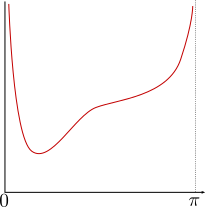
(a) The case $d\in[0,\sqrt{1-4H^{2}})$

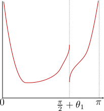
(b) The case $d=\sqrt{1-4H^{2}}$, $H\neq\tfrac{1}{2\sqrt{2}}$

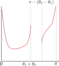
(c) The case $d>\sqrt{1-4H^{2}}$

Figure 2. $H$-surfaces invariant by hyperbolic translation.

• if $d\in[0,\sqrt{1-4H^{2}}),$ then $u^{H}_{d}$ is defined for any $\theta\in(0,\pi)$ and

  $$\underset{\theta\to 0^{+}}{\lim}u^{H}_{d}=\underset{\theta\to\pi^{-}}{\lim}u^{H}_{d}=+\infty$$

  (see Figure 2(a));

• if $d=\sqrt{1-4H^{2}},$ then $u^{H}_{d}$ is defined for any $\theta\in\left(0,\tfrac{\pi}{2}+\theta_{1}\right)\cup\left(\tfrac{\pi}{2}+\theta_{1},\pi\right)$ and

  $$\begin{array}[]{ccccl}\underset{\theta\to 0^{-}}{\lim}u^{H}_{d}(\theta)&=&\underset{\theta\to\pi^{+}}{\lim}u^{H}_{d}(\theta)&=&+\infty,\\ \underset{\theta\to\left(\tfrac{\pi}{2}+\theta_{1}\right)^{-}}{\lim}\dot{u}^{H}_{d}(\theta)&=&\underset{\theta\to\left(\tfrac{\pi}{2}+\theta_{1}\right)^{+}}{\lim}\dot{u}^{H}_{d}(\theta)&=&+\infty,\end{array}$$

  (see Figure 2(b));

• if $d>\sqrt{1-4H^{2}},$ then $u^{H}_{d}$ is defined for any $\theta\in(0,\theta_{1}+\theta_{2}]\cup[\pi-(\theta_{2}-\theta_{1}),\pi)$, that is, it has two disconnected component, and

  $$\begin{array}[]{ccccl}\underset{\theta\to 0^{-}}{\lim}u^{H}_{d}(\theta)&=&\underset{\theta\to\pi^{+}}{\lim}u^{H}_{d}(\theta)&=&+\infty\\ \underset{\theta\to(\theta_{1}+\theta_{2})^{-}}{\lim}\dot{u}^{H}_{d}(\theta)&=&\underset{\theta\to(\pi-(\theta_{2}-\theta_{1}))^{+}}{\lim}\dot{u}^{H}_{d}(\theta)&=&+\infty\end{array}$$

  (see Figure 2(c)).

In [2, Theorem 3.4] the authors state that, when $d=\sqrt{1-4H^{2}}$,

$$\underset{\theta\to(\tfrac{\pi}{2}+\theta_{1})^{-}}{\lim}u^{H}_{d}(\theta),\qquad\underset{\theta\to(\tfrac{\pi}{2}+\theta_{1})^{+}}{\lim}u^{H}_{d}(\theta)$$

are finite and that, when $d>\sqrt{1-4H^{2}}$,

$$\underset{\theta\to(\theta_{1}+\theta_{2})^{-}}{\lim}u^{H}_{d}(\theta),\qquad\underset{\theta\to(\pi-(\theta_{2}-\theta_{1}))^{+}}{\lim}u^{H}_{d}(\theta)$$

are finite. In the following proposition, we focus on the case $d=\tfrac{1}{\sqrt{2}}$ and prove that in this case the statement cannot be true. We also prove in Proposition 3.2 that, for any $H\in\left(0,\tfrac{1}{2\sqrt{2}}\right)\cup\left(\tfrac{1}{2\sqrt{2}},\tfrac{1}{2}\right)$, there exists $d>\sqrt{1-4H^{2}}$ such that either

$$\underset{\theta\to(\theta_{1}+\theta_{2})^{-}}{\lim}u^{H}_{d}(\theta)\textrm{ or }\underset{\theta\to(\pi-(\theta_{2}-\theta_{1}))^{+}}{\lim}u^{H}_{d}(\theta)$$

diverges to $+\infty$ or $-\infty$.

Proposition 3.1.

If $d=\sqrt{1-4H^{2}}$ and $H=\tfrac{1}{2\sqrt{2}},$ then

$$\begin{array}[]{ccc}\underset{\theta\to\left(\tfrac{\pi}{2}+\theta_{1}\right)^{-}}{\lim}u^{H}_{d}(\theta)=+\infty&\textrm{and}&\underset{\theta\to\left(\tfrac{\pi}{2}+\theta_{1}\right)^{+}}{\lim}u^{H}_{d}(\theta)=-\infty.\end{array}$$

Proof.

Let $\Sigma_{H}$ be the vertical cylinder of constant mean curvature $H$ parametrized by

$$\Sigma_{H}(\phi,t)=\left(\cos\left(\theta_{1}+\tfrac{\pi}{2}\right)e^{\phi},\sin\left(\theta_{1}+\tfrac{\pi}{2}\right)e^{\phi},t\right).$$

Suppose that there exist $k\in\mathbb{R},$ such that $\underset{\theta\to\theta_{0}^{-}}{\lim}u^{H}_{d}(\theta)=k,$ then $\Theta^{H}_{d}(\phi,\theta)$ and $\Sigma_{H}(\varphi,t)$ are two surfaces of constant mean curvature $H,$ with mean curvature vector pointing in the same direction, which are tangent along the curve $(\cos(\theta_{0})e^{\phi},\sin(\theta_{0})e^{\phi},k)$ (see Figure 3). This contradicts the Boundary Maximum Principle.

Figure 3. $\Sigma_{H}$ is tangent to $\Omega^{H}_{d}$ if $\underset{\theta\to\left(\theta_{1}+\tfrac{\pi}{2}\right)^{-}}{\lim}u^{H}_{d}(\theta)=k.$

The same argument is used to prove that $\underset{\theta\to\theta_{0}^{+}}{\lim}u^{H}_{d}(\theta)=-\infty,$ and concludes the proof. ∎

Proposition 3.2.

If $H>\tfrac{1}{2\sqrt{2}},$ there exists $d^{*}\in(\sqrt{1-4H^{2}},+\infty)$ such that

$$\underset{\theta\to(\pi-(\theta_{2}-\theta_{2}))^{+}}{\lim}u^{H}_{d^{*}}(\theta)=-\infty.$$

If $H<\tfrac{1}{2\sqrt{2}},$ there exists $d^{*}\in(\sqrt{1-4H^{2}},+\infty)$ such that

$$\underset{\theta\to(\theta_{1}+\theta_{2})^{-}}{\lim}u^{H}_{d^{*}}(\theta)=+\infty.$$

Proof.

Notice that

$$\underset{d\to+\infty}{\lim}(\theta_{1}+\theta_{2})=0,\qquad\underset{d\to+\infty}{\lim}(\pi-(\theta_{2}-\theta_{1}))=\pi$$

and that

$$\underset{d\to\sqrt{1-4H^{2}}}{\lim}(\theta_{1}+\theta_{2})=\underset{d\to\sqrt{1-4H^{2}}}{\lim}(\pi-(\theta_{2}-\theta_{1}))=\tfrac{\pi}{2}+\arcsin(2H)=\pi-\arccos(2H).$$

If $H>\tfrac{1}{2\sqrt{2}},$ then

$$\arccos(2H)+\tfrac{\pi}{2}>\pi-\arccos(2H)=\tfrac{\pi}{2}+\arcsin(2H).$$

Hence, by continuity, there exists $d^{*}\in(\sqrt{1-4H^{2}},+\infty)$ such that

$$\pi-(\theta_{2}-\theta_{1})=\arccos(2H)+\tfrac{\pi}{2}.$$

Analogously, if $H<\tfrac{1}{2\sqrt{2}},$ then

$$\arccos(2H)+\tfrac{\pi}{2}<\pi-\arccos(2H)=\tfrac{\pi}{2}+\arcsin(2H),$$

and, by continuity, there exists $d^{*}\in(\sqrt{1-4H^{2}},+\infty)$ such that

$$\theta_{1}+\theta_{2}=\arccos(2H)+\tfrac{\pi}{2}.$$

The result follows applying the same argument of Proposition 3.1. ∎

To study the asymptotic behaviour, we compute the maximum of the height growth of each graph with respect to the slide $\left\{t=0\right\}$ as a function of geodesic radius of the base $\mathbb{H}^{2}.$ The study of $\mathcal{R}^{H}_{d}$ is easy, since the growth function $v_{d}^{H}$ is already defined as a function of the geodesic radius of $\mathbb{H}^{2}.$ So, we only need to study its behaviour for $\rho\to\infty.$ An easy computation implies that

$$\dot{v}^{H}_{d}(\rho)\simeq\frac{2H\sqrt{1+\tau^{2}}}{\sqrt{1-4H^{2}}}+\frac{2(d+4d\tau^{2}+8H(-1+4H^{2})\tau^{2})}{(1-4H^{2})^{\tfrac{3}{2}}\sqrt{1+4\tau^{2}}}e^{-\rho}+o\left(e^{-\rho}\right),$$

and integrating this function we get

$$v^{H}_{d}(\rho)\simeq\frac{2H\sqrt{1+\tau^{2}}}{\sqrt{1-4H^{2}}}\rho-\frac{2(d+4d\tau^{2}+8H(-1+4H^{2})\tau^{2})}{(1-4H^{2})^{\tfrac{3}{2}}\sqrt{1+4\tau^{2}}}e^{-\rho}+o\left(e^{-\rho}\right).$$ (3.3)

In a similar way we study the growth of $\Theta^{H}_{d}$. First we have to notice that growth function $u^{H}_{d}$ is not written with respect to the geodesic radius of the base, so we need to use the change $\theta(\rho)=2\arctan\left(e^{\rho}\right).$ This implies that

$$\dot{u}^{H}_{d}(\rho)=\frac{2e^{\rho}}{1+e^{2\rho}}\left(\frac{|d-2H\cot\left(2\arctan\left(e^{\rho}\right)\right)|\sqrt{1+4\tau^{2}\cos^{2}\left(2\arctan\left(e^{\rho}\right)\right)}}{\sqrt{1-\left(d\sin\left(2\arctan\left(e^{\rho}\right)\right)-2H\cos\left(2\arctan\left(e^{\rho}\right)\right)\right)^{2}}}-2\tau\right).$$

In this case, since we are allowing $\rho$ to be negative, we need study separately the growth function for $\rho\to+\infty$ and $\rho\to-\infty$. By a simple computation, we get

$$\dot{u}^{H}_{d}(\rho)\simeq\begin{cases}\begin{array}[]{ll}\frac{2H\sqrt{1+\tau^{2}}}{\sqrt{1-4H^{2}}}+\left(-4\tau+d\sqrt{\frac{1+4\tau^{2}}{(1-4H^{2})^{3}}}\right)e^{-\rho}+o(e^{-\rho})&\textrm{for }\rho\to+\infty,\\ -\frac{2H\sqrt{1+\tau^{2}}}{\sqrt{1-4H^{2}}}+\left(-4\tau+d\sqrt{\frac{1+4\tau^{2}}{(1-4H^{2})^{3}}}\right)e^{\rho}+o(e^{-\rho})&\textrm{for }\rho\to-\infty,\end{array}\end{cases}$$

and integrating this function, we get that

$$u^{H}_{d}(\rho)\simeq\frac{2H\sqrt{1+\tau^{2}}}{\sqrt{1-4H^{2}}}|\rho|+Ke^{-|\rho|}+o(e^{-|\rho|})$$ (3.4)

for $|\rho|\to+\infty$ and $K=4\tau-d\sqrt{\frac{1+4\tau^{2}}{(1-4H^{2})^{3}}}$ if $\rho>0$ and $K=-4\tau+d\sqrt{\frac{1+4\tau^{2}}{(1-4H^{2})^{3}}}$ if $\rho<0.$

The last thing to check is the asymptotic relation between $\mathcal{U}$ and $\mathcal{S}$, that will allow us to compare $\mathcal{R}^{H}_{d_{1}}$ and $\Theta^{H}_{d_{2}}.$ To do so, we use (2.3) to write $\mathcal{U}$ in the half-space model $\mathcal{H}$ and compare it to $\mathcal{S},$ that is $\left\{t=0\right\}.$ So, in the cylinder model $\mathcal{C},$ we parametrize $\mathcal{U}$, that is $\left\{t=0\right\},$ by

$$\mathcal{U}(x,y)=\left(\frac{-1+x^{2}+y^{2}}{x^{2}+(y+1)^{2}},\frac{-2x}{x^{2}+(y+1)^{2}},0\right),$$

with $(x,y)\in\left\{\mathbb{R}^{2}\mid y>0\right\}.$ Hence, the image of $\mathcal{U}$ by the isometry (2.3) is

$$(\psi^{-1}\circ\mathcal{U})(x,y)=\left(x,y,4\tau\arctan\left(\tfrac{x}{y+1}\right)\right)$$

(see [1] for more details).

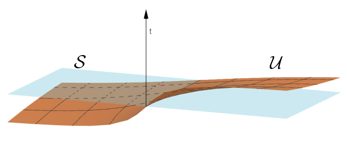
Figure 4. The umbrella surface $\mathcal{U}$ in the half-space model $\mathcal{H}$.

In particular we have that the vertical distance between $\mathcal{U}$ and $\mathcal{S}$ is bounded (see Figure 4). This implies that, fixed $H\in\left[0,\tfrac{1}{2}\right),$ for any $d_{1},d_{2}\in\mathbb{R}$ the asymptotic vertical distance between $\mathcal{R}^{H}_{d_{1}}$ and $\Theta^{H}_{d_{2}}$ is bounded by a constant.

4. A new model for $\mathbb{E}(-1,\tau)$

In this subsection we describe a new cylindrical model and a new half-space model for $\mathbb{E}(-1,\tau),$ in which the slice $\left\{t=0\right\}$ has constant sectional curvature $0<H<\tfrac{1}{2}$.

In general, if $U\subset\mathbb{R}^{2}$ is a simply connected domain endowed with the conformal metric $\lambda^{2}(x,y)(dx^{2}+dy^{2})$ and $U\times\mathbb{R}$ is such that $\pi\colon U\times\mathbb{R}\to U$ is a unitary Killing submersion with bundle curvature $\tau$, then $U\times\mathbb{R}$ is endowed with the metric

$$\lambda^{2}(dx^{2}+dy^{2})+[\lambda(a(x,y)dx+b(x,y)dy)+dt]^{2},$$

where $a,b\in\mathcal{C}^{\infty}(U)$ satisfy

$$\frac{(\lambda b)_{x}-(\lambda a)_{y}}{2\lambda^{2}}=\tau.$$

If $\Sigma=(x,y,d(x,y)),$ for $d\in\mathcal{C}^{\infty}(U),$ is a complete graph, the map

$$\begin{array}[]{rccc}\mathcal{I}\colon&U\times\mathbb{R}&\to&U\times\mathbb{R}\\ &(x,y,t)&\mapsto&(x,y,t-d(x,y))\end{array}$$ (4.1)

is an isometry that allows to see $\Sigma$ as the graph $\left\{z=0\right\}$ in $U\times\mathbb{R}$ endowed with the metric

$$\lambda^{2}(dx^{2}+dy^{2})+[\lambda(a^{\prime}(x,y)dx+b^{\prime}(x,y)dy)+dt]^{2}$$

The relation between $a$ and $a^{\prime}$ and $b$ and $b^{\prime}$ is given by the uniqueness of Killing submersions (see [10, Theorem 2.6]) and reads

$$b^{\prime}=\frac{b+d_{y}}{\lambda},\qquad a^{\prime}=\frac{a+d_{x}}{\lambda}.$$

For any $H\in\left[0,\tfrac{1}{2}\right]$, applying this technique to $\mathbb{E}(-1,\tau),$ described with the cylindrical model $\mathcal{C},$ and the surface $\mathcal{R}^{H}_{-2H}(\rho,\theta)$, we get that $\mathbb{E}(-1,\tau)$ is isometric to $\Omega\times\mathbb{R},$ endowed with the metric

$$ds^{2}=\lambda_{\mathcal{C}}(x,y)(dx^{2}+dy^{2})+\left[\lambda_{\mathcal{C}}(x,y)\left[a_{\mathcal{C}}^{H}(x,y)dx+b_{\mathcal{C}}^{H}(x,y)dy\right]+dt\right]^{2},$$ (4.2)

with

$$\begin{array}[]{ll}a_{\mathcal{C}}^{H}(x,y)&=2y\tau+2Hx\sqrt{\frac{1+4(x^{2}+y^{2})\tau^{2}}{1-4H^{2}(x^{2}+y^{2})}},\\ b_{\mathcal{C}}^{H}(x,y)&=-2x\tau+2Hy\sqrt{\frac{1+4(x^{2}+y^{2})\tau^{2}}{1-4H^{2}(x^{2}+y^{2})}},\end{array}$$

where the graph $\left\{t=0\right\}$ is rotationally invariant and has constant mean curvature $H.$

In this model the mean curvature equation of the graph of a function $u\colon U\subset\Omega\to\mathbb{R}$ is given by

$$H(u)=\tfrac{1}{2}\mathop{\rm div}\nolimits\left(\frac{Gu}{\sqrt{1+\|Gu\|^{2}}}\right),$$ (4.3)

where $\mathop{\rm div}\nolimits(\cdot)$ and $\|\cdot\|$ are respectively the divergence and norm of $\mathbb{H}^{2}$ with the Poincaré disk metric $\lambda_{\mathcal{C}}^{2}(dx^{2}+dy^{2}),$ and

$$Gu=\tfrac{1}{\lambda_{\mathcal{C}}^{2}}\left[(u_{x}-\lambda_{\mathcal{C}}a_{\mathcal{C}}^{H})\partial_{x}+(u_{y}-\lambda_{\mathcal{C}}b_{\mathcal{C}}^{H})\partial_{y}\right].$$

For any $H\in\left[0,\tfrac{1}{2}\right]$, applying this technique to $\mathbb{E}(-1,\tau),$ described with the half-space model $\mathcal{H},$ and the surface $\Theta_{0}^{H}(\varphi,\theta)$, we get that $\mathbb{E}(-1,\tau)$ is isometric to $\Omega\times\mathbb{R},$ endowed with the metric

$$ds^{2}=\lambda_{\mathcal{H}}(x,y)(dx^{2}+dy^{2})+\left[\lambda_{\mathcal{H}}(x,y)\left[a_{\mathcal{H}}^{H}(x,y)dx+b_{\mathcal{H}}^{H}(x,y)dy\right]+dt\right]^{2},$$ (4.4)

with

$$\begin{array}[]{ll}a_{\mathcal{H}}^{H}(x,y)&=\frac{2y}{x^{2}+y^{2}}\left((x^{2}+y^{2}+y)\tau+\frac{Hx\sqrt{y^{2}+x^{2}(1+4\tau^{2})}}{\sqrt{(1-4H^{2})x^{2}+y^{2}}}\right),\\ b_{\mathcal{H}}^{H}(x,y)&=\frac{2x}{x^{2}+y^{2}}\left(-y\tau-\frac{Hx\sqrt{y^{2}+x^{2}(1+4\tau^{2})}}{\sqrt{(1-4H^{2})x^{2}+y^{2}}}\right),\end{array}$$

where the graph $\left\{t=0\right\}$ is invariant by hyperbolic translation and has constant mean curvature $H.$

In this model the mean curvature equation of the graph of a function $u\colon U\subset\Omega\to\mathbb{R}$ is given by

$$H(u)=\tfrac{1}{2}\mathop{\rm div}\nolimits\left(\frac{Gu}{\sqrt{1+\|Gu\|^{2}}}\right),$$ (4.5)

where $\mathop{\rm div}\nolimits(\cdot)$ and $\|\cdot\|$ are respectively the divergence and norm of $\mathbb{H}^{2}$ with the half-plane metric $\lambda_{\mathcal{H}}^{2}(dx^{2}+dy^{2}),$ and

$$Gu=\tfrac{1}{\lambda_{\mathcal{H}}^{2}}\left[(u_{x}-\lambda_{\mathcal{H}}a_{\mathcal{H}}^{H})\partial_{x}+(u_{y}-\lambda_{\mathcal{H}}b_{\mathcal{H}}^{H})\partial_{y}\right].$$

Regardless of the model we are using, if $D\subset\Omega$ is an open domain and $u\in\mathcal{C}^{2}(D)\cap\mathcal{C}^{0}(\partial D)$ satisfies $H(u)=H\in\mathbb{R},$ then, integrating $\mathop{\rm div}\nolimits\left(\frac{Gu}{\sqrt{1+\|Gu\|^{2}}}\right)$ gives

$$2H\mathcal{A}(D)=\int_{\partial D}\left\langle{\frac{Gu}{\sqrt{1+\|Gu\|^{2}}},\nu}\right\rangle,$$ (4.6)

where $\mathcal{A}(D)$ is the hyperbolic area of $D$ and $\nu$ is the outer normal to $\partial D.$ The integral in the right side of the equation is called flux of $u$ across $\partial D.$ If $\gamma\subset\partial D$ is diffeomorphic to a segment we can define the flux of $u$ across $\gamma$ as follows:

Definition 4.1.

Let $\Gamma\subset D$ any smooth curve such that $\gamma\cup\Gamma$ bound a simply connected domain $\Delta_{\Gamma}.$ Then we define the flux of $u$ across $\gamma$ as

$$\mathrm{Flux}_{u}(\gamma)=2H\mathcal{A}(\Delta_{\Gamma})-\int_{\Gamma}\left\langle{\frac{Gu}{\sqrt{1+\|Gu\|^{2}}},\nu}\right\rangle$$

Notice that this definition does not depend on the choice of $\Gamma.$

We now state two Lemmas that we need to construct the barriers and to prove Theorem 7.5. The proof is analogous to the case $\tau=0,$ proved in [9, Section 5].

Lemma 4.2.

Let $u$ be such that $\mathcal{P}(u)=0$ in a bounded domain $D$ and let $\Gamma$ be a piecewise $\mathcal{C}^{1}$ curve in $\partial D.$ Then:

$$2H\mathcal{A}(D)=\int_{\partial D}\left\langle{\frac{Gu}{\sqrt{1+\|Gu\|^{2}}},\nu}\right\rangle\,\textrm{and }\left|\int_{\Gamma}\left\langle{\frac{Gu}{\sqrt{1+\|Gu\|^{2}}},\nu}\right\rangle\right|\leq|\Gamma|.$$

Lemma 4.3.

Let $D$ be a domain bounded in part by an arc $\gamma$ and let $\left\{u_{n}\right\}$ be a sequence of solutions of $\mathcal{P}(u_{n})=0$ in $D,$ such that each $\left\{u_{n}\right\}$ is continuous on $\gamma.$ Then

1. if the sequence tends to $+\infty$ uniformly on compact subsets of $\gamma$ while remaining uniformly bounded on compact subsets of $D,$ we have

   $$\underset{n\to\infty}{\lim}\int_{\gamma}\left\langle{\frac{Gu_{n}}{\sqrt{1+\|Gu_{n}\|^{2}}},\nu}\right\rangle=|\gamma|;$$

2. if the sequence tends to $-\infty$ uniformly on compact subsets of $\gamma$ while remaining uniformly bounded on compact subsets of $D,$ we have

   $$\underset{n\to\infty}{\lim}\int_{\gamma}\left\langle{\frac{Gu_{n}}{\sqrt{1+\|Gu_{n}\|^{2}}},\nu}\right\rangle=-|\gamma|.$$

5. Construction of the barriers

In this section we build the asymptotic barriers that will be used in the proof of the Main Theorems. For $E(-1,\tau),$ we consider the half-space model with $\left\{t=0\right\}$ having constant mean curvature $H$, described by $\Omega\times\mathbb{R}$ endowed with the metric (4.5). The study done in Section 3 implies that, in this model, the results of Propositions 3.1 and 3.2 can be read as follows:

Theorem 5.1.

For any $c\in\mathbb{R},$ let $\gamma_{c}\subset\Omega$ be the curve $\gamma_{c}(t)=\left(\frac{-2H}{\sqrt{1-4H^{2}}}t+c,t\right)_{t>0}$ and denote by

$$D^{-}_{c}=\left\{(x,y)\in\Omega\,|\,x<\frac{-2H}{\sqrt{1-4H^{2}}}y+c\right\},\,D^{+}_{c}=\left\{(x,y)\in\Omega\,|\,x>\frac{-2H}{\sqrt{1-4H^{2}}}y+c\right\}.$$

Then

• If $H=\tfrac{1}{2\sqrt{2}},$ in $D^{\pm}_{c}$ there exists a solution $\omega_{\pm}$ to the asymptotic Dirichlet problem

  $$\begin{cases}\begin{array}[]{ll}\mathcal{P}(\omega_{\pm})=0&\textrm{in }D^{\pm}_{c},\\ \omega_{\pm}=0&\textrm{in }\left\{y=0\right\},\\ \omega_{\pm}=\pm\infty&\textrm{in }\gamma_{c}.\end{array}\end{cases}$$

• If $\tfrac{1}{2\sqrt{2}}<H<\tfrac{1}{2},$ in $D^{-}_{c}$ there exists a solution $\omega_{-}$ to the asymptotic Dirichlet problem

  $$P(\gamma_{c},-)=\begin{cases}\begin{array}[]{ll}\mathcal{P}(\omega_{-})=0&\textrm{in }D^{-}_{c},\\ \omega_{-}=0&\textrm{in }\left\{y=0\right\},\\ \omega_{-}=-\infty&\textrm{in }\gamma_{c}.\end{array}\end{cases}$$

• If $0<H<\tfrac{1}{2\sqrt{2}},$ in $D^{+}_{c}$ there exists a solution $\omega_{+}$ to the asymptotic Dirichlet problem

  $$P(\gamma_{c},+)=\begin{cases}\begin{array}[]{ll}\mathcal{P}(\omega_{+})=0&\textrm{in }D^{+}_{c},\\ \omega_{+}=0&\textrm{in }\left\{y=0\right\},\\ \omega_{+}=+\infty&\textrm{in }\gamma_{c}.\end{array}\end{cases}$$

So, it remains to prove that, when $\tfrac{1}{2\sqrt{2}}<H<\tfrac{1}{2},$ the problem $P(\gamma_{c},+)$ admits a solution $\omega_{+}$ and that, when $0<H<\tfrac{1}{2\sqrt{2}},$ the problem $P(\gamma_{c},-)$ admits a solution $\omega_{-}$.

First, we recall a useful result proved in [20, Theorem 3.3]:

Theorem 5.2.

Let $D\subset\mathbb{H}^{2}$ be a domain bounded in part by a $\mathcal{C}^{2}$ arc $\gamma$ and let $u\in\mathcal{C}^{2}(D)$ be a solution of $\mathcal{P}(u)=0.$ If $u$ tend to $+\infty$ for any approach to interior points of $\gamma,$ then $\gamma$ has geodesic curvature $\kappa_{g}(\gamma)=2H,$ while if $u$ tends to $-\infty$ for any approach to interior points of $\gamma,$ then $\gamma$ has geodesic curvature $\kappa_{g}(\gamma)=-2H.$

Denoting by $\theta_{1}=\arcsin\left(2H\right)$, let $\gamma_{c}^{H}\subset\Omega$ be the curve $\left(\cos\left(\theta_{1}+\frac{\pi}{2}\right)t+c,\sin\left(\theta_{1}+\frac{\pi}{2}\right)t\right)_{t>0},$ and define

$$D^{-}_{H,c}= \left\{(x,y)\in\Omega\,|\,x<\cot\left(\theta_{1}+\frac{\pi}{2}\right)y+c\right\},$$

$$D^{+}_{H,c}= \left\{(x,y)\in\Omega\,|\,x>\cot\left(\theta_{1}+\frac{\pi}{2}\right)y+c\right\}.$$

In this model, the surface $\Theta^{H}_{\sqrt{1-4H^{2}}}$ has two components $\Theta^{-}$ and $\Theta^{+},$ defined respectively in $D^{-}_{H,c}$ and $D^{+}_{H,c}.$ Up to apply a vertical translation, $\Theta^{-}$ is the graph of a negative function $s^{-}\in\mathcal{C}^{\infty}(D^{-}_{H,c})$ satisfying

$$\begin{cases}\begin{array}[]{ll}\mathcal{P}(s^{-})=0&\textrm{in }D^{-}_{H,c},\\ s^{-}=0&\textrm{in }\left\{y=0\right\},\\ \frac{\partial s^{-}}{\partial\nu}=-\infty&\textrm{in }\gamma^{H}_{c},\end{array}\end{cases}$$

where $\nu$ is the outer normal to $\gamma^{H}_{c}.$ Analogously, $\Theta^{+}$ is the graph of a positive function $s^{+}\in\mathcal{C}^{\infty}(D^{+}_{H,c})$ satisfying

$$\begin{cases}\begin{array}[]{ll}\mathcal{P}(s^{+})=0&\textrm{in }D^{+}_{H,c},\\ s^{+}=0&\textrm{in }\left\{y=0\right\},\\ \frac{\partial s^{+}}{\partial\nu}=+\infty&\textrm{in }\gamma^{H}_{c}.\end{array}\end{cases}$$

Using $s^{+}$ and $s^{-}$ as barriers we can prove the following result.

Theorem 5.3.

If $\tfrac{1}{2\sqrt{2}}<H<\tfrac{1}{2},$ then there exists a solution $\omega_{+}$ to the problem $P(\gamma_{c},+).$ If $0<H<\tfrac{1}{2\sqrt{2}},$ then there exists a solution $\omega_{-}$ to the problem $P(\gamma_{c},-).$

Proof.

Suppose first that $\tfrac{1}{2\sqrt{2}}<H<\tfrac{1}{2}.$ A simple computation implies that $\gamma_{c}\subset D^{-}_{H,c}.$ Let $B(r)$ be the geodesic disks centered in $\gamma_{c}(1)$ with geodesic radius $r$ and denote by $D^{+}_{r}=D^{+}\cap B(r).$ For any $n\in\mathbb{N},$ [3, Theorem 1] implies the existence of a solution $\omega^{n}_{r}$ to the problem

$$\begin{cases}\begin{array}[]{ll}\mathcal{P}(\omega^{n}_{r})=0&\textrm{in }D^{+}_{r},\\ \omega^{+}_{n}=n&\textrm{in }\partial D^{+}_{r}\cap\partial D^{+},\\ \omega^{+}_{n}=0&\textrm{in }\partial B(r)\cap D^{+}.\end{array}\end{cases}$$

The maximum principle implies that, if we fix $n,$ for any $r_{1}>r_{2}$ we get $\omega^{n}_{r_{1}}>\omega^{n}_{r_{2}}$ in $D^{+}_{r_{2}}.$

We need to prove that, for any $r\in\mathbb{R}^{+}$ and $n\in\mathbb{N},$ we have $\omega^{n}_{r}<s^{+}$ in $D^{+}_{H,c}\cap D^{+}_{r}.$ Assume that for some $n$ and $r,$ $\omega^{n}_{r}>s^{+}$ in a subdomain of $D^{+}_{H,c}\cap D^{+}_{r}.$ Let $a\in\mathbb{R}^{+}$ be a sufficiently large constant such that $\omega^{n}_{r}-a<s^{+}$ in $D^{+}_{H,c}\cap D^{+}_{r}.$ Sending $a\to 0,$ the maximum principle implies that there exists a positive constant $a^{*}>0$ such that $\omega^{n}_{r}-a^{*}\leq s^{+}$ in $\partial(D^{+}_{H,c}\cap D^{+}_{r})$ and the points where $\omega^{n}_{r}-a^{*}=s^{+}$ are contained in $\gamma^{H}_{c}.$ We get a contradiction since $\frac{\partial s^{+}}{\partial\nu}=+\infty$ while $\frac{\partial(\omega^{n}_{r}-a^{*})}{\partial\nu}<+\infty$ in $\gamma^{H}_{c}.$

So we get that, fixed $n\in\mathbb{N},$ $\left\{\omega^{n}_{r}\right\}_{r}$ is an increasing sequence converging to a solution $\omega^{n}$ of the problem

$$\begin{cases}\begin{array}[]{ll}\mathcal{P}(\omega^{n})=0&\textrm{in }D^{+},\\ \omega^{n}=n&\textrm{in }\gamma_{c},\\ \omega^{n}=0&\textrm{in }\left\{y=0\right\}.\end{array}\end{cases}$$

Notice that $\left\{\omega^{n}\right\}$ is an increasing sequence of solutions of $\mathcal{P}(\omega^{n})=0$ bounded below by $\left\{t=0\right\}$ in all $D^{+}$ and above by $s^{+}$ in $D^{+}_{H,c}.$ Hence, applying the Monotone Convergence Theorem, there exists $\omega_{+}=\underset{n\to\infty}{\lim}\omega^{n}$ defined in the convergence set $\mathcal{U}\subset D^{+}.$ Since in $D^{+}_{H,c}$ the sequence has an upper bound, the divergence set $\mathcal{V}$ will be contained in $\overline{D^{+}}\setminus D^{+}_{H,c}.$ Theorem 5.2 implies that $\partial\mathcal{V}\cap\partial\mathcal{U}$ is the union of smooth arcs with constant geodesic curvature $2H$, each one convex towards $\mathcal{U}.$

Since $\gamma_{c}$ is the only smooth curve of constant geodesic curvature $2H$ contained in $\overline{D^{+}}\setminus D^{+}_{H,c}$ with the right orientation, the result follows by proving that $\partial\mathcal{V}\cap\partial\mathcal{U}$ is smooth.

Assume first that two arcs $\gamma_{1},\gamma_{2}\subset\partial\mathcal{V}\cap\partial\mathcal{U}$ meet at a convex corner $p$ of $\mathcal{U}.$ Let $p_{1}$ (resp. $p_{2}$) a point in $\gamma_{1}$ (resp. $\gamma_{2}$) sufficiently close to $p,$ such that $\left|\tilde{\gamma}_{1}\right|=\left|\tilde{\gamma}_{2}\right|=\varepsilon$, where $\tilde{\gamma}_{1}$ (resp. $\tilde{\gamma}_{2}$) is the part of $\gamma_{1}$ (resp. $\gamma_{2}$) between $p$ and $p_{1}$ (resp. $p_{2}$) and let $\gamma_{3}$ be the geodesic arc connecting $p_{1}$ and $p_{2}$ (notice that $\gamma_{3}\subset\mathcal{U}$ since $p$ is a convex corner of $\partial\mathcal{U}$). We denote by $\Delta$ the triangle bounded by $\tilde{\gamma}_{1}\cup\tilde{\gamma}_{2}\cup\gamma_{3}.$ Equation (4.6) and Definition 4.1 implies that

$$2H\mathcal{A}(\Delta)=\mathrm{Flux}_{\omega^{n}}(\tilde{\gamma}_{1})+\mathrm{Flux}_{\omega^{n}}(\tilde{\gamma}_{2})+\mathrm{Flux}_{\omega^{n}}(\gamma_{3}),$$ (5.1)

while Lemma 4.3 implies that

$$\lim_{n\to\infty}\mathrm{Flux}_{\omega^{n}}(\tilde{\gamma}_{1})=|\tilde{\gamma}_{1}|=\varepsilon,\qquad\lim_{n\to\infty}\mathrm{Flux}_{\omega^{n}}(\tilde{\gamma}_{2})=|\tilde{\gamma}_{2}|=\varepsilon.$$ (5.2)

From (5.1), (5.2) and Lemma 4.2, we deduce that

$$2H\mathcal{A}(\Delta)\geq 2\varepsilon-|\gamma_{3}|.$$

Equivalently, we have

$$\frac{2H\mathcal{A}(\Delta)}{|\gamma_{3}|}\geq\frac{2\varepsilon}{|\gamma_{3}|}-1.$$

A contradiction is given by the fact that $\underset{\varepsilon\to 0}{\lim}\frac{\mathcal{A}(\Delta)}{|\gamma_{3}|}=0,$ while the left-hand side of the equation remains uniformly positive.

Assume now that two arcs $\gamma_{1},\gamma_{2}\subset\partial\mathcal{V}\cap\partial\mathcal{U}$ meet at a convex corner $p$ of $\mathcal{V}.$ Let $p_{1}$ be a point in the interior of $\gamma_{1},$ let $\Gamma$ be a curve in $\mathcal{U}$ joining $p$ and $p_{1}$ and denote by $\Delta$ the domain bounded by $\Gamma\cup\gamma_{1}.$ In particular $u=(\omega_{+})_{|\Delta}$ is a solution to the Dirichlet problem

$$\begin{cases}\begin{array}[]{ll}\mathcal{P}(u)=0&\textrm{in }\Delta,\\ u=\omega_{+}&\textrm{in }\Gamma,\\ u=+\infty&\textrm{in }\gamma_{1}.\end{array}\end{cases}$$

Applying an ambient isometry $\varphi,$ such that $\varphi(\cdot)=\cdot^{*},$ we can assume that $p$ is in the interior of $\Delta^{*}$ and $\overline{\Gamma}$ is in the interior of $\mathcal{U},$ in particular we have that $\mathcal{U}\cap\Delta^{*}\neq\emptyset$ and $\mathcal{V}\cap\Delta^{*}\neq\emptyset.$ Hence, for $a>0$ sufficiently large, the maximum principle implies that $\varphi(u)+a>\omega^{n}$ in $\Delta^{*}$ for any $n\in\mathbb{N}.$ So, the Monotone Convergence Theorem implies that $\Delta^{*}\subset\mathcal{U},$ but this contradicts the fact that $\mathcal{V}\cap\Delta^{*}\neq\emptyset.$

Suppose now that $0<H<\tfrac{1}{2\sqrt{2}}.$ A simple computation implies that both $\gamma_{c}$ and $\tilde{\gamma}_{c}$ are contained in $D^{-}_{H,c}$ (where $\tilde{\gamma}_{c}$ is the reflection of $\gamma_{c}$ with respect to the geodesic $\left\{x=c\right\}$ in $\mathbb{H}^{2}$). We denote by $\tilde{D}$ the reflection of $D^{+}$ with respect to the geodesic $\left\{x=c\right\}$ (clearly $D^{-}_{H,c}\subset\tilde{D}$). Let $B(r)$ be the geodesic disks centered in $\tilde{\gamma}_{c}(1)$ of geodesic radius $r$ and denote by $D^{-}_{r}=\tilde{D}\cap B(r).$ For any $n\in\mathbb{N},$ [3, Theore 1] implies the existence of the solution $\omega^{n}_{r}$ to the problem

$$\begin{cases}\begin{array}[]{ll}\mathcal{P}(\omega^{n}_{r})=0&\textrm{in }D^{-}_{r},\\ \omega^{+}_{n}=-n&\textrm{in }\partial D^{-}_{r}\cap\partial\tilde{D},\\ \omega^{+}_{n}=0&\textrm{in }\partial B(r)\cap\tilde{D}.\end{array}\end{cases}$$

As above, it is easy to show that for any $n\in\mathbb{N},$ there exists $\omega^{n}=\underset{r\to\infty}{\lim}\omega^{n}_{r}$ and that $\left\{\omega^{n}\right\}_{n}$ is a strictly decreasing sequence of solutions of $\mathcal{P}(\omega^{n})=0$ defined in $\tilde{D}.$ Hence, applying the Monotone Convergence Theorem, there exists $\omega_{-}=\underset{n\to\infty}{\lim}\omega^{n}$ defined in the convergence set $\mathcal{U}\subset D^{+}.$ Since in $D^{+}_{H,c}$ the sequence has an upper bound, the divergence set $\mathcal{V}$ will be contained in $\overline{\tilde{D}}\setminus D^{-}_{H,c}.$ Theorem 5.2 implies that $\partial\mathcal{V}\cap\partial\mathcal{U}$ is the union of smooth arcs of constant geodesic curvature $2H$, each one convex towards $\mathcal{U}.$

Again, since $\gamma_{c}$ is the only smooth curve of constant geodesic curvature $2H$ contained in $\overline{\tilde{D}}\setminus D^{-}_{H,c}$ with the right orientation, the result follows by proving that $\partial\mathcal{V}\cap\partial\mathcal{U}$ is smooth.

If $\gamma_{1},\gamma_{2}\subset\partial\mathcal{V}\cap\partial\mathcal{U}$ are two arcs meeting at a convex corner $p$ of $\mathcal{V},$ we use the same argument as above. So, assume that two arcs $\gamma_{1},\gamma_{2}\subset\partial\mathcal{V}\cap\partial\mathcal{U}$ meet at a convex corner $p$ of $\mathcal{U}.$ Let $p_{1}$ (resp. $p_{2}$) a point in $\gamma_{1}$ (resp. $\gamma_{2}$) sufficiently close to $p,$ such that $\left|\tilde{\gamma}_{1}\right|=\left|\tilde{\gamma}_{2}\right|=\varepsilon$, where $\tilde{\gamma}_{1}$ (resp. $\tilde{\gamma}_{2}$) is the part of $\gamma_{1}$ (resp. $\gamma_{2}$) between $p$ and $p_{1}$ (resp. $p_{2}$) and let $\gamma_{3}$ be the geodesic arc connecting $p_{1}$ and $p_{2}$ (notice that $\gamma_{3}\subset\mathcal{U}$ since $p$ is a convex corner of $\partial\mathcal{U}$). We denote by $\Delta$ the triangle bounded by $\tilde{\gamma}_{1}\cup\tilde{\gamma}_{2}\cup\gamma_{3}.$ Equation 4.6 and Definition 4.1 implies that

$$2H\mathcal{A}(\Delta)=\mathrm{Flux}_{\omega^{n}}(\tilde{\gamma}_{1})+\mathrm{Flux}_{\omega^{n}}(\tilde{\gamma}_{2})+\mathrm{Flux}_{\omega^{n}}(\gamma_{3}),$$ (5.3)

while Lemma 4.3 implies that

$$\lim_{n\to\infty}\mathrm{Flux}_{\omega^{n}}(\tilde{\gamma}_{1})=-\varepsilon,\qquad\lim_{n\to\infty}\mathrm{Flux}_{\omega^{n}}(\tilde{\gamma}_{2})=-\varepsilon.$$ (5.4)

From (5.1), (5.2) and Lemma 4.2, we deduce that, for $\varepsilon$ sufficiently small,

$$2H\mathcal{A}(\Delta)\leq-2\varepsilon+|\gamma_{3}|<0,$$

which gives a contradiction and completes the proof. ∎

If we describe $\mathbb{E}(-1,\tau)$ with the model $\Omega\times\mathbb{R}$ endowed with the metric (4.2), applying rotations with respect to the $t$-axis and parabolic translations, Theorems 5.1 and 5.3 guarantee the existence of asymptotic barriers as follows:

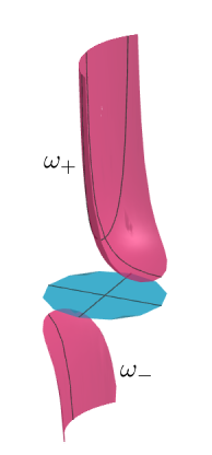
Figure 5. Asymptotic barriers.

Theorem 5.4.

Let $\gamma\subset\Omega$ be a curve of constant geodesic curvature $2H$ which separates the disk $\Omega$ in two connected domains. We denote by $D^{+}$ the convex component and $D^{-}$ the other one. Then, there exists two functions $\omega_{+}$ and $\omega_{-}$ solving the Dirichlet problems

$$\begin{cases}\begin{array}[]{ll}\mathcal{P}(\omega_{+})=0&\textrm{in }D^{+},\\ \omega_{+}=+\infty&\textrm{in }\gamma,\\ \omega_{+}=f^{+}&\textrm{in }\partial D^{+}\setminus\gamma,\end{array}\end{cases}\,\textrm{and}\,\begin{cases}\begin{array}[]{ll}\mathcal{P}(\omega_{-})=0&\textrm{in }D^{-},\\ \omega_{-}=-\infty&\textrm{in }\gamma,\\ \omega_{-}=f^{-}&\textrm{in }\partial D^{-}\setminus\gamma,\end{array}\end{cases}$$

where $f^{+}\in\mathcal{C}^{\infty}(\partial D^{+}\setminus\gamma)$ and $f^{-}\in\mathcal{C}^{\infty}(\partial D^{-}\setminus\gamma)$ are bounded functions.

6. Existence of entire $H$-graphs

In this section we consider the model of $\mathbb{E}(-1,\tau)$ given by $\Omega\times\mathbb{R}$ endowed with the metric in (4.2), in which $\left\{t=0\right\}$ is a rotational surface of constant mean curvature $H\in\left(0,\tfrac{1}{2}\right).$ In this setting we prove the existence of $H$-graph having prescribed asymptotic boundary value. The proof is inspired to the one of [16, Theorem 4], where the authors prove an analogous result for $\tau=H=0.$ We point out that an existence result for subcritical CMC graphs in $\mathbb{H}^{2}\times\mathbb{R}$ was already prove in [7], we prove a similar result avoiding the use of Scherk graphs over ideal domains in its proof.

Theorem 6.1.

Let $\Gamma$ be a rectifiable curve in $\partial\Omega\times\mathbb{R}$, that is the vertical graph of the function $f\in\mathcal{C}(\partial\Omega)$. Then, there exists an entire $H$-graph having $\Gamma$ as asymptotic boundary. Such graph is unique.

Proof.

Assume first that $\Gamma$ is differentiable. For $n\in\mathbb{N}$, let $D_{n}\subset\Omega$ be the disk centered at the origin with Euclidean radius $1-\tfrac{1}{n+1},$ so that $\left\{D_{n}\right\}_{n}$ is an exhaustion of $\Omega.$ Since $\partial D_{n}$ has geodesic curvature greater than $2H$ for any $n\in\mathbb{N},$ for any $g\in\mathcal{C}(\partial D_{n})$, there exists an $H$-graph $u\in\mathcal{C}^{2}(D_{n})$ such that $u\equiv g$ in $\partial D_{n}.$ Let $\eta_{n}\colon\partial D_{n}\to\partial\Omega$ be such that $\eta_{n}(x,y)=\left(\tfrac{n+1}{n}x,\tfrac{n+1}{n}y\right)$ and $f_{n}=f\circ\eta_{n}.$ Hence, $f_{n}(\partial D_{n})$ is a sequence of curves lying between $\left\{t=\min\,f\right\}$ and $\left\{t=\max\,f\right\}$ and converging to $\Gamma$ for $n\to\infty.$ Denote by $u_{n}$ the solution of the Dirichlet problem for constant mean curvature $H$ in $D_{n}$ with $f_{n}$ as boundary values and by $M_{n}$ its graph. The maximum principle implies that $\min\,f\leq u_{n}\leq\max\,f$ for any $n\in\mathbb{N},$ thus, Compactness Theorem implies that there exists a subsequence converging to a solution $u\colon\Omega\to\mathbb{R}$ uniformly on compact subsets of $\Omega$, and denote by $M$ its graph. We have that $\Gamma$ is contained in the asymptotic boundary $\partial M$ of $M$ by construction, so it remain to prove that if $p\in\partial\Omega\times\mathbb{R}\setminus\Gamma,$ then $p\notin\partial M.$ Assume that there exist $p\in\partial M$ lying below $\Gamma,$ without loss of generality we can assume $p=(1,0,f(1,0)-2\varepsilon).$ Let $\varepsilon_{1}>0$ be such that $\underset{q\in\partial\Omega_{\varepsilon_{1}}}{\max}(f((1,0))-f(q))<\varepsilon,$ where $\partial\Omega_{\varepsilon_{1}}=\left\{(x,y)\in\partial\Omega\mid|y|<\varepsilon_{1}\right\}.$ Let $\gamma$ be the curve of constant geodesic curvature $2H$ that has $\partial(\partial\Omega_{\varepsilon_{1}})$ and that is concave with respect to the domain bounded by $\gamma$ and $\partial\Omega_{\varepsilon_{1}}.$ Let $k\in\mathbb{R}$ be a constant such that $\omega_{-}(1,0)+k=f(1,0)-\varepsilon.$ Notice that if $\epsilon_{1}$ is sufficiently small, up to apply a rotation with respect to the $t$-axis, we get that $\omega_{-}+k<f$ in $\partial\Omega_{\varepsilon_{1}}.$ By construction, the graph of $\omega_{-}+k$ lies below $\Gamma_{n}$ for any $n$ sufficiently large, and so the maximum principle implies that $M_{n}$ is above the graph of $\omega_{-}+k$. Hence the limit of $M_{n}$, that is $M,$ cannot contain $p$ in its asymptotic boundary. If $p$ lies above $\Gamma$, we can apply the same argument using $\omega_{+}$ instead of $\omega_{-}$. The uniqueness follows by the maximum principle.

Now, if $\Gamma$ is rectifiable, we consider two families of differentiable curves approximating $\Gamma$ respectively from above and from below, and use the argument in [17, Correction 4(a)] and this conclude the proof. ∎

Remark 6.2.

The result of this theorem is consistent with the Slab Theorem in [8]. Indeed, moving back to the classical cylinder model $\mathcal{C}$ with $\left\{t=0\right\}$ being rotational and minimal, we have that all the solutions given applying Theorem 6.1 are asymptotic to the entire rotational $H$-graph, that is, they diverge to $+\infty$ approaching the asymptotic vertical boundary of $\mathcal{C}.$ Furthermore, the previous result shows that a half-space Theorem analogous to [18, Theorem 1] and [12, Theorem 3] cannot be proven for $H<\tfrac{1}{2}$ and that the hypothesis of [14, Theorem 2] are sharp.

7. Asymptotic Jenkins–Serrin result

Again we consider the model of $\mathbb{E}(-1,\tau)$ given by $\Omega\times\mathbb{R}$ endowed with the metric in (4.2), in which $\left\{t=0\right\}$ is a rotational surface of constant mean curvature $H\in\left(0,\tfrac{1}{2}\right).$ In this section we prove a Jenkins–Serrin type result for subcritical constant mean curvature graphs over unbounded domains of $\mathbb{H}^{2}.$ When $\tau=0$ this result was proven by Mazet, Rodriguez and Rosenberg (see [13, Theorems 4.9, 4.12]) for $H=0$ and by Folha and Melo (see [6, Theorems 3.1, 3.2]) for $0<H<\tfrac{1}{2}$ when the asymptotic boundary of the domain consists only of a finite number of isolated points of the asymptotic boundary of $\mathbb{H}^{2}.$ We extend these results to the case $\tau\neq 0$ allowing the asymptotic boundary of the domains to contain part of the asymptotic boundary of $\mathbb{H}^{2}.$

Definition 7.1 (Jenkins–Serrin domain).

A domain $\mathcal{D}\subset\mathbb{H}^{2}$ is called a Jenkins–Serrin domain if its boundary $\partial_{\infty}\mathcal{D}$ consists of a finite number of arcs $A_{i}$ and $B_{i}$ of constant geodesic curvature $2H$ and $-2H$ respectively, a finite number of arcs $C_{i}$ of geodesic curvature $k_{g}(C_{i})\geq 2H$ and a finite number of open arcs $D_{i}$ at $\partial_{\infty}\mathbb{H}^{2},$ together with their endpoints, which are called the vertices of $\mathcal{D}.$

We say that a Jenkins–Serrin domain $\mathcal{D}$ is admissible if

1. neither two $A_{i}$ or two $B_{i}$ meets at a convex corner of $\mathcal{D},$ nor at an asymptotic vertex;

2. denoting by $B_{i}^{*}$ the reflection of $B_{i}$ in $\mathbb{H}^{2}$ with respect to the geodesic passing through the endpoints of $B_{i}$, for any $i\in I,$ the interior of $B_{i}^{*}$ does not intersect $\overline{\mathcal{D}}.$

If $\mathcal{D}$ is an admissible Jenkins–Serrin domain, we call extended Jenkins–Serrin domain the domain $\mathcal{D}^{*}$ whose boundary $\partial_{\infty}\mathcal{D}^{*}$ consists of the union of the arcs $A_{i}$, $B_{i}^{*}$, $C_{i}$ and $D_{i}.$

Remark 7.2.

Condition (A) of admissibility is a necessary condition that can be deduced by the proof of Theorem 5.3. Condition (B), is necessary to define the extended Jenkins–Serrin domain, where is possible to solve a Dirichlet problem with finite boundary data.

Definition 7.3 (Jenkins–Serrin Problem).

Let $f_{i}\in\mathcal{C}(C_{i})$ and $g_{i}\in\mathcal{C}^{0}(D_{i}).$ Then, we call Jenkins–Serrin Problem the Dirichlet Problem

$$\mathcal{P}_{JS}(\mathcal{D}):=\begin{cases}\begin{array}[]{ll}u=+\infty&\textrm{in }\cup A_{i},\\ u=-\infty&\textrm{in }\cup B_{i},\\ u=f_{i}&\textrm{in }C_{i},\\ u=g_{i}&\textrm{in }D_{i}.\end{array}\end{cases}$$

Definition 7.4 (Inscribed polygon).

Let $\mathcal{D}$ be an admissible domain. We say that $P$ is an admissible inscribed polygon if $P\subset\mathcal{D}\cup\partial\mathcal{D},$ its edges have constant geodesic curvature $\pm 2H$ and all the vertices of $P$ are vertices of $\mathcal{D}.$

For each ideal vertex $p_{i}$ of $\mathcal{D}$ at $\partial_{\infty}\mathbb{H}^{2},$ we consider a horocycle $H_{i}$ at $p_{i}.$ Assume $H_{i}$ is small enough so that it does not intersect bounded edges of $\partial_{\infty}\mathcal{D}$ and $H_{i}\cap H_{j}=\emptyset$ for every $i\neq j.$ Let $F_{i}$ be the convex horodisk with boundary $H_{i}.$ Each $A_{i}$ meets exactly two horodisks. Denote by $\tilde{A}_{i}$ the compact arc of $A_{i}$ which is the part of $A_{i}$ outside the two horodisks; we define $|A_{i}|=$ as the length if $\tilde{A}_{i}.$ Let $P\subset\mathcal{D}$ be an inscribed polygon and denote by $\mathcal{D}_{P}\subset\mathcal{D}$ the domain bounded by $P.$ For each arc $\eta_{j}\in P,$ we define $\tilde{\eta}_{j}$ and $|\eta_{j}|$ in the same way.

$$\gamma(P)=\sum_{j\in J}|\eta_{j}|,\qquad\alpha(P)=\sum_{A_{i}\subset P}|A_{i}|\quad\textrm{and}\quad\beta(P)=\sum_{B_{i}\in P}|B_{i}|.$$

For any family of horocycles $\mathcal{H}=\left\{H_{i}\right\},$ denote by $F_{i}$ the convex horodisk bounded by $H_{i},$ $\tilde{\mathcal{D}}_{P}=\underset{i}{\bigcup}(\mathcal{D}_{P}\cup F_{i})$ and $\mathcal{D}_{P}^{\mathcal{H}}=\mathcal{D}_{P}\setminus\tilde{\mathcal{D}}_{P}$ and we define

$$\tilde{A}(\mathcal{D}_{P}):=\mathcal{A}(\mathcal{D}_{P}^{\mathcal{H}})+\mathcal{A}(\tilde{\mathcal{D}}_{P}).$$

Notice that this definition makes sense, since $\mathcal{A}(\tilde{\Omega})$ is finite (see [6, Section 3]).

Theorem 7.5.

Let $\mathcal{D}$ be an admissible Jenkins–Serrin domain. Assume that both $\left\{C_{i}\right\}$ and $\left\{D_{i}\right\}$ are empty. Then, there exists a solution to the Dirichlet problem $\mathcal{P}_{JS}(\mathcal{D})$ if and only if for some choice of horocycles at the vertices we have

$$\alpha(\partial\mathcal{D})=\beta(\partial\mathcal{D})+2H\tilde{\mathcal{A}}(\mathcal{D}),$$

and for any inscribed polygon $P,$

$$\alpha(P)<\gamma(P)+2H\tilde{\mathcal{A}}(\mathcal{D}_{P})\qquad\textrm{and}\qquad\beta(P)>\gamma(P)-2H\tilde{\mathcal{A}}(\mathcal{D}_{P}).$$ (7.1)

If $\mathcal{D}$ is relatively compact, the solution is unique up to vertical translation.

If either $\left\{C_{i}\right\}$ or $\left\{D_{i}\right\}$ is not empty, there exists a solution to $\mathcal{P}_{JS}(\mathcal{D})$ if and only if for some choice of horocycles at the vertices, the inequalities in (7.1) are satisfied for any polygon $P$ inscribed in $\mathcal{D}.$ If $\mathcal{D}$ is relatively compact, the solution is unique.

Sketch of the proof.

Since the Jenkins–Serrin result relies on the existence of upper and lower barriers and computation of areas and lengths in the base $\mathbb{H}^{2},$ the proof of the theorem above will be equal to the one of [9, Theorems 7.11 and 7.12] (for $\mathcal{D}$ relatively compact) and [6, Theorems 3.1 and 3.2] (for $\mathcal{D}$ unbounded and $\left\{D_{i}\right\}=\emptyset$).

If $\mathcal{D}$ is unbounded and $\left\{D_{i}\right\}\neq\emptyset,$ we built a sequence of solutions as done in the proof of [13, Theorem 4.9] for the minimal case. Consider the extended Jenkins–Serrin domain $\mathcal{D^{*}}.$ For $n\in\mathbb{N}$, let $\mathbb{D}_{n}\subset\Omega$ be the disk centered at the origin with Euclidean radius $1-\tfrac{1}{n+1},$ and let $\mathcal{D}_{n}=\mathbb{D}_{n}\cap\mathcal{D}^{*},$ so that $\left\{\mathcal{D}_{n}\right\}_{n}$ is an exhaustion of $\mathcal{D}^{*}.$ Let $\eta_{n}\colon\partial\mathbb{D}_{n}\to\partial\Omega$ be such that $\eta_{n}(x,y)=\left(\tfrac{n+1}{n}x,\tfrac{n+1}{n}y\right),$ denote by $D_{i,n}=\eta_{n}^{-1}(D_{i})$ and define $g_{i,n}=g_{i}\circ\eta_{n}\colon D_{i,n}\to\mathbb{R}.$ Denote by $C_{i,n}=C_{i}\cap\mathbb{D}_{n},$ $A_{i,n}=A_{i}\cap\mathbb{D}_{n}$ and $B_{i,n}=B_{i}^{*}\cap\mathbb{D}_{n},$ so that $\partial\mathcal{D}_{n}=\cup A_{i,n}\cup B_{i,n}\cup C_{i,n}\cup D_{i,n}\cup\Gamma_{n},$ where $\Gamma_{n}=(\partial\mathbb{D}_{n}\cap\mathcal{D}^{*})\setminus(\underset{i}{\cup}D_{i,n}).$ For any $m,n\in\mathbb{N},$ we can solve the Dirichlet problem

$$\begin{cases}\begin{array}[]{ll}\mathcal{P}(u_{m,n})=0&\textrm{in }\mathcal{D}_{n},\\ u_{m,n}=m&\textrm{in }A_{i,n},\\ u_{m,n}=-m&\textrm{in }B_{i,n},\\ u_{m,n}=f_{i,m}&\textrm{in }C_{i,n},\\ u_{m,n}=g_{i,n,m}&\textrm{in }D_{i,n},\\ u_{m,n}=0&\textrm{in }\Gamma_{n},\end{array}\end{cases}$$

where the function $f_{i,m}$ (resp. $g_{i,n,m}$) denotes the function $f_{i}$ (resp. $g_{i,n}$) truncated above and below by $m$ and $-m,$ respectively. Notice that, by the maximum principle we have that $-m\leq u_{m,n}\leq m.$ Hence, as in the proof of Main Theorem 6.1, the existence of the barriers $\omega_{+}$ and $\omega_{-}$ and the compactness theorem implies that, up to pass to a subsequence, $\left\{u_{m,n}\right\}$ converges uniformly on compact subsets of $\mathcal{D}^{*}$ to an $H$-graph $u_{m}\colon\mathcal{D}^{*}\to\mathbb{R}$ with boundary data

$$\begin{cases}\begin{array}[]{ll}\mathcal{P}(u_{m})=0&\textrm{in }\mathcal{D}_{n},\\ u_{m}=m&\textrm{in }A_{i},\\ u_{m}=-m&\textrm{in }B_{i},\\ u_{m}=f_{i,m}&\textrm{in }C_{i},\\ u_{m}=g_{i,m}&\textrm{in }D_{i},\end{array}\end{cases}$$

where the function $f_{i}$ (resp. $g_{i,m}$) denotes again the function $f_{i,m}$ (resp. $g_{i}$) truncated above and below by $m$ and $-m,$ respectively. For any $D_{i}\subset\partial\mathcal{D}$ there exists a curve $\hat{D}_{i}$ having the same endpoints points of $D_{i}$ and geodesic curvature $\kappa_{g}(\hat{D}_{i})\geq 2H$ such that the domain $\hat{\mathcal{D}}_{i}$ bounded by $D_{i}\cup\hat{D}_{i}$ is concave and $\hat{D}_{i}\subset\mathcal{D}.$ Using $\omega_{+}$ and $\omega_{-},$ we can find two functions $\hat{g}_{i}^{+},\hat{g}_{i}^{-}\in\mathcal{C}(\hat{D}_{i})$ such that $\hat{g}_{i}^{-}<u_{m}<\hat{g}_{i}^{+}$ in $\hat{D}_{i},$ for any $m\in\mathbb{N}.$ Notice that $\mathcal{D}\setminus(\underset{i}{\cup}\hat{\mathcal{D}}_{i})$ is an admissible Jenkins–Serrin domain with $\left\{D_{i}\right\}=\emptyset$ there exist $u^{+},u^{-}\in\mathcal{C}^{\infty}(\hat{\mathcal{D}})$ satisfying

$$\begin{cases}\begin{array}[]{ll}\mathcal{P}(u^{+})=0,&\textrm{in }\mathcal{D}\setminus(\underset{i}{\cup}\hat{\mathcal{D}}_{i}),\\ u^{+}=+\infty&\textrm{in }A_{i},\\ u^{+}=-\infty&\textrm{in }B_{i},\\ u^{+}=f_{i}&\textrm{in }C_{i},\\ u^{+}=\hat{g}^{+}_{i}&\textrm{in }\hat{D}_{i}\\ \end{array}\end{cases}\textrm{ and}\quad\begin{cases}\begin{array}[]{ll}\mathcal{P}(u^{-})=0,&\textrm{in }\mathcal{D}\setminus(\underset{i}{\cup}\hat{\mathcal{D}}_{i}),\\ u^{-}=+\infty&\textrm{in }A_{i},\\ u^{-}=-\infty&\textrm{in }B_{i},\\ u^{-}=f_{i}&\textrm{in }C_{i},\\ u^{-}=\hat{g}^{-}_{i}&\textrm{in }\hat{D}_{i}.\\ \end{array}\end{cases}$$

The Maximum principle finally implies that $u^{-}\leq u_{m}\leq u^{+}$ in $\mathcal{D}\setminus(\underset{i}{\cup}\hat{\mathcal{D}}_{i}),$ for any $m\in\mathbb{N}.$ Hence, applying the compactness theorem, we get that $\left\{u_{m}\right\}$ admits a subsequence that converges to the solution $u$ of the Jenkins–Serrin problem in every compact subset of $\mathcal{D}.$ The fact that $u$ converges to the function $g_{i}$ in $D_{i}$ follows by applying the same argument of the proof of Theorem 6.1. ∎

References

- [1] Jesús Castro-Infantes. On the asymptotic Plateau problem in . J. Math. Anal. Appl. 507, no. 2 (2022), 125831.
- [2] Qing Cui, Albetã Mafra and Carlos Peñafiel. Immersed hyperbolic and parabolic screw motion surfaces in the space . Geom. Dedicata 178 (2015), 297–322.
- [3] Marcos Dajczer and Jorge Herbert de Lira. Killing graphs with prescribed mean curvature and Riemannian submersions. Ann. Inst. Henri Poincare (C) Anal. Non Lineaire 26, no. 3 (2009), 763–775.
- [4] Andrea Del Prete, José M. Manzano and Barbara Nelli. The Jenkins–Serrin problem in -manifolds with a Killing vector field. Preprint (available at arXiv:2306.12195) (2023).
- [5] M. Eichmair, J. Metzger. Jenkins–Serrin-type results for the Jang equation. J. Differential Geom., 102 (2016), 207–242.
- [6] Abigail Folha and Sofia Melo. The Dirichlet problem for constant mean curvature graphs in over unbounded domains. Pac. J. Math. 251, no. 1 (2011), 37–65.
- [7] Abigail Folha and Harold Rosenberg. Entire constant mean curvature graphs in . Pac. J. Math. 316, no. 2 (2022), 307–333.
- [8] Laurent Hauswirth, Ana Menezes and Magdalena Rodríguez. Slab theorem and halfspace theorem for constant mean curvature surfaces in . Rev. Mat. Iberoam. 39, no. 1 (2023), 307–320.
- [9] Laurent Hauswirth, Harold Rosenberg and Joel Spruck. Infinite Boundary Value Problems for Constant Mean Curvature Graphs in and . Am. J. Math. 131 no. 1 (2009), 195–226.
- [10] Ana M. Lerma and José M. Manzano. Compact stable surfaces with constant mean curvature in Killing submersions. Ann. Mat. Pura Appl. 196 (2017), 1345–1364.
- [11] José M Manzano. On the classification of Killing submersions and their isometries. Pac. J. Math 270, no. 2 (2014), 367–392.
- [12] Laurent Mazet. The half space property for cmc graphs in . Calc. Var. Partial Differ. Equ. 52 (2015), 661–680.
- [13] Laurent Mazet, M Magdalena Rodríguez, and Harold Rosenberg. The Dirichlet problem for the minimal surface equation, with possible infinite boundary data, over domains in a Riemannian surface. Proc. Lond. Math. Soc. 102, no. 6 (2011), 985–1023.
- [14] Laurent Mazet and Gabriela A. Wanderley. A half-space theorem for graphs of constant mean curvature in . Ill. J. Math. 59, no. 1 (2015), 43–53.
- [15] Sofia Melo. Minimal graphs in over unbounded domains. Bull. Braz. Math. Soc., New Series 45 (2014), 91–116.
- [16] Barbara Nelli and Harold Rosenberg. Minimal surfaces in . Bull. Braz. Math. Soc., New Series 33, no. 2 (2002), 263–292.
- [17] Barbara Nelli and Harold Rosenberg. Erratum to “Minimal surfaces in ”. Bull. Braz. Math. Soc., New Series 38 (2007), 661–664.
- [18] Barbara Nelli and Ricardo Sa Earp. A halfspace theorem for mean curvature surfaces in . J. Math. Anal. Appl. 365 (2010), 167–170.
- [19] Carlos Peñafiel. Invariant surfaces in and applications. Bull. Braz. Math. Soc., New Series 43 (2012), 545–578.
- [20] Harold Rosenberg, Rabah Souam and Eric Toubiana. General curvature estimates for stable -surfaces in 3-manifolds applications. J. Differ. Geom. 84, no. 3 (2010), 623–648.
- [21] Ricardo Sa Earp. Parabolic and hyperbolic screw motion surfaces in . J. Aust. Math. Soc. 85, no. 1 (2008), 113–143.
- [22] Ricardo Sa Earp and Eric Toubiana. Screw motion surfaces in and . Ill. J. Math 49, no.4, (2005), 1323–1362.