The Pairwise Matching Design is Optimal under Extreme Noise and Assignments

Abstract

We consider the general performance of the difference-in-means estimator in an equally-allocated two-arm randomized experiment under common experimental endpoints such as continuous (regression), incidence, proportion, count and uncensored survival. We consider two sources of randomness: the subject-specific assignments and the contribution of unobserved subject-specific measurements. We then examine mean squared error (MSE) performance under a new, more realistic simultaneous tail criterion. We prove that the pairwise matching design of Greevy et al. (2004) performs best asymptotically under this criterion when compared to other blocking designs. We also prove that the optimal design must be less random than complete randomization and more random than any deterministic, optimized allocation. Theoretical results are supported by simulations in all five response types.

Keywords: experimental design, optimal design, pairwise matching, blocking, incidence endpoint, count endpoint

1 Background

We consider a classic problem: a randomized experiment with $2n$ subjects (individuals, participants or units). The experiment has two arms (treatments, manipulations or groups), which we will call treatment and control denoted $T$ and $C$. The goal herein is to infer the causal sample average treatment effect (SATE) and thus, we randomize subjects thereby assigning them into the two groups.

Formally defined, the randomization (allocation or an assignment) is a vector $\boldsymbol{w}:=\left[w_{1},\ldots,w_{2n}\right]^{\top}$ whose entries indicate whether the subject received $T$ (coded numerically as +1) or $C$ (coded numerically as -1) and thus this vector is an element in $\left\{-1,+1\right\}^{2n}$. The only liberty the experimenter has is to choose the entries of $\boldsymbol{w}$. The random process that results in the allocation of the $2n$ subjects to the two arms is termed an experimental design (strategy, algorithm, method or procedure.) Experimental design may be viewed as a random draw (most often with equal probability) from a set of $\boldsymbol{w}$’s; this process we denote as random variable $\boldsymbol{W}$.

After the experiment concludes, we measure one outcome (response or endpoint) of interest for the $2n$ subjects denoted $\boldsymbol{y}=\left[y_{1},\ldots,y_{2n}\right]^{\top}$ which is of a general data type: either continuous, incidence, count or uncensored survival and we use these values along with the assignment $\boldsymbol{w}$ to perform inference for the SATE.

If nothing is known about the subjects before assignment, the typical “gold-standard” design is the balanced complete randomization design (BCRD, Wu, , 1981, p. 1171). This design has $\binom{2n}{n}$ allocations each that satisfy the balance constraint $\sum_{i}w_{i}=0$. Each allocation is then chosen with equal probability.

If the subjects have observed characteristics, other designs which incorporate these a priori measurements are more popular. We now assume each subject has $p$ real-valued observed subject-specific covariates (measurements, features or characteristics) collected into a row vector denoted $\boldsymbol{x}_{i}$ for the $i$th subject. The setting we investigate is where all $\boldsymbol{x}_{i}$’s are known beforehand and considered fixed. This non-sequential setting was studied by Fisher, (1925) when assigning treatments to agricultural plots and is still of great importance today. In fact, this setting is found in “many phase I studies [that] use ‘banks’ of healthy volunteers … [and] … in most cluster randomised trials, the clusters are identified before treatment is started” (Senn, , 2013, page 1440). The more common sequential experimental setting where subjects arrive one-by-one and must be assigned on the spot (hence all $\boldsymbol{x}_{i}$’s are not seen beforehand), will be left for future work.

When, observing subject-specific characteristics, should BCRD still be employed? The consensus is “no” due to a reason that was noted immediately by Fisher: under some unlucky $\boldsymbol{w}$’s there are large differences in the distribution of observed covariates between the two arms. The amount of covariate value heterogeneity between groups we term observed imbalance. This observed imbalance creates bias during estimation from the perspective of any single $\boldsymbol{w}$ but it is more canonical to say that it creates variance from the perspective of considering all $\boldsymbol{w}$’s.

Thus, “restricted” designs are employed which restrict the allowable $\boldsymbol{w}$’s in an effort to minimize the observed imbalance among the two arms. Restricted designs have a long literature once again starting with Fisher, (1925, p. 251) who wrote “it is still possible to eliminate much of the …heterogeneity, and so increase the accuracy of our [estimator], by laying restrictions on the order in which the strips are arranged”. Here, he introduced the block design, a restricted design still popular today, especially in clinical trials. Another early mitigation approach can be found in Student, (1938, p. 366) who wrote that after an unlucky, highly imbalanced randomization, “it would be pedantic to [run the experiment] with [an assignment] known beforehand to be likely to lead to a misleading conclusion”. His solution is for “common sense [to prevail] and chance [be] invoked a second time”. In foregoing the first assignment and rerandomizing to find a better assignment, all allocations worse than a predetermined threshold of observed imbalance are eliminated. This classic strategy has been rigorously investigated only recently (Morgan and Rubin, , 2012; Li et al., , 2018) in the case of equal allocation. Another idea is to allocate treatment and control among similar subjects by using a pairwise matching (PM) design (Greevy et al., , 2004) which creates $n$ pairs of subjects which minimize an overall average covariate distance within pair. In each pair, one subject receives T and the other receives C with equal probability.

One may wonder about the “optimal” restricted design strategy. The design $\boldsymbol{W}$ is a multivariate Bernoulli random variable has $2^{2n}-1$ parameters, an exponentially large number (Teugels, , 1990, Section 2.3). Finding the optimal design is thus tantamount to solving for exponentially many parameters using only the $2n$ observations, a hopelessly unidentifiable task. Thus, to find an “optimal” design, the space of designs must be limited. One way of limiting the space of designs is to do away with any notion of randomization whatsoever and instead compute a deterministic perfect balance (PB) optimal allocation; this is a design with two allocation vectors $\boldsymbol{w}_{*}$ and the allocation where its subjects switched arms $-\boldsymbol{w}_{*}$. An early advocate of this approach was Smith, (1918) and a good review of classic works advocating this approach such as Kiefer and Wolfowitz, (1959) is given in Steinberg and Hunter, (1984, Chapter 3). A particularly edgy advocate of PB is Harville, (1975) who penned an article titled “Experimental Randomization: Who Needs It?”.

We have introduced thus far a continuum of designs from the most random (BCRD) and thus has the highest expected observed imbalance to the least random (one optimized, deterministic $\boldsymbol{w}$) which has the lowest expected observed imbalance. Other designs such as blocking, rerandomization and PM are thus located somewhere in the middle of these two extremes. A natural question to ask is do these two considerations (degree of randomness and degree of observed imbalance) trade off among each other? Yes, since randomization balances both observed and unobserved covariates, the less random a design is, the more likely the unobserved covariate measurements will be imbalanced. This imbalance in unseen characteristics has the potential to wreak havoc on estimation error. Thus, the assumptions about these unobserved covariates and how they are incorporated into the experimental performance metric become critically important.

This trade-off was investigated in Kapelner et al., (2021) for the case of a continuous outcome. They analyzed three unobserved covariate scenarios (I) nature provides the worst possible values of unobserved covariates, (II) the unobserved covariates are random noise that will be averaged over (i.e., colloquially, “margined out”) and (III) the unobserved covariates are random noise but the concern is about values of these unobserved covariates that produce terrible estimator performance. Naturally, there was a threefold answer to what the optimal design would be. Under (I), the experimenter should never sacrifice any randomness and thus BCRD is optimal; under (II), the experimenter can sacrifice all randomness and employ the deterministic design (although unpalatable to modern ears); and under (III), the experimenter should sacrifice some randomness and use a design in between the two extremes. Azriel et al., (2023), henceforth called our “previous work”, extended these results to general response models and unequal allocation. They found that the unequal randomization case admits the same results. But response types that are not continuous are more complicated. Under (I), the problem is intractable but when limited to the space of all block designs, then BCRD is the optimal design. Under (II), the deterministic design is still optimal but impossible as it requires knowledge of the latent parameters within the response model. Under (III), the problem is again intractable but when limited to the space of all block designs, then block designs with few blocks are optimal (a number of blocks of order between $n^{1/4}$ and $n$).

Our work herein extends our previous work by examining (III) under a different tail criterion, one that we believe to be more realistic. In our previous work, the tail was defined as a large quantile (e.g. 95%, 99%, etc) over the observed covariates of the expected squared error of the estimator over assignments. This tail criterion is realistic in that it considers values of observed covariates that can lead to poor performance. However, the inner expectation over all assignments is troublesome. In any single experiment, only one $\boldsymbol{w}$ is realized. Herein, we define the tail criterion to be the quantile over the joint distribution of the possible unobserved covariates simultaneous with the possible design assignments. We seek designs that minimize these tail events that will ruin an experiment. Our optimal design results are found to be fundamentally different.

When examining performance gauged by this simultaneous tail criterion, locating the optimal design is, as expected, unidentifiable. But, when limiting our design space to blocking designs, we find PM to be asymptotically optimal. We define our experimental setting formally in Section 2, discuss criterions of performance and theoretical results in Section 3, provide simulation evidence of our results in Section 4 and conclude in Section 5.

2 Problem Setup

The problem setup is identical to our previous work’s setup section. We cannot reprint it here because it will be flagged as plagiarism. Sorry for making you click on the link. We must however reprint Table 1 below because we reference it later in this work.

Response type name	$\mathcal{Y}$	Model Name	Common $\mu_{T,i}$ and $\mu_{C,i}$	$\Theta$
Continuous	$\mathbb{R}$	Linear	$\beta_{0}+\boldsymbol{\beta}^{\top}\boldsymbol{x}_{i}+\beta_{T}w_{i}$	$\mathbb{R}$
Incidence	$\left\{0,1\right\}$	Log Odds	$\left(1+e^{-(\beta_{0}+\boldsymbol{\beta}^{\top}\boldsymbol{x}_{i}+\beta_{T}w_{i})}\right)^{-1}$	$(0,1)$
Proportion	$(0,1)$	Linear
Count	$\left\{0,1,\ldots\right\}$	Log Linear	$e^{\beta_{0}+\boldsymbol{\beta}^{\top}\boldsymbol{x}_{i}+\beta_{T}w_{i}}$	$(0,\infty)$
Survival	$(0,\infty)$

Table 1: Response types considered where $\beta$’s are unknown parameters.

3 Analyzing Designs

It is impossible to employ the MSE as the criterion in which we compare different designs since $\boldsymbol{v}$ is not observed (as $\boldsymbol{z}_{T}$ and $\boldsymbol{z}_{C}$ are not observed). Our previous work has design recommendation results for (I) the criterion of the worst case MSE, i.e. the worst $\boldsymbol{z}_{T}$ and $\boldsymbol{z}_{C}$; and results under (II) the “mean MSE”, i.e. the average $\boldsymbol{z}_{T}$ and $\boldsymbol{z}_{C}$. The worst case MSE design only considers the most improbable tail event and thus is too conservative. The mean MSE design is either intractable or might lead to idiosyncratic $\boldsymbol{z}_{T}$’s and $\boldsymbol{z}_{C}$’s that introduce large mean squared error with non-negligible probability. Thus, we wish to analyze a criterion that balances these two extremes; one such criterion is a tail event MSE. Our previous paper defined the “single quantile tail criterion” which measures this tail event,

$$\text{Quantile}_{\boldsymbol{Z}_{T},\boldsymbol{Z}_{C}}\left[\mathbb{M}\text{SE}_{\boldsymbol{W}}\left[\hat{\tau}\right],q\right].$$ (1)

In order to define the quantile operator above, we must formally let $\boldsymbol{Z}_{T}$ and $\boldsymbol{Z}_{C}$ be the vector random variables that generate the $\boldsymbol{z}_{T}$ and $\boldsymbol{z}_{C}$ vectors respectively (quantities that are canonically denoted with the Greek letter epsilon). We assume $\mathbb{E}\left[\boldsymbol{Z}_{T}\right]=\mathbb{E}\left[\boldsymbol{Z}_{C}\right]=\boldsymbol{0}_{n}$ and that the components in $\boldsymbol{Z}_{T}$ are independent, the components of $\boldsymbol{Z}_{C}$ are independent and the components of the former and latter are mutually independent. Although the distributional form of both $\boldsymbol{Z}_{T}$ and $\boldsymbol{Z}_{C}$ are implicitly constrained by the response type specified by $\mathcal{Y}$, we do not make any formal distributional assumptions beyond vague moment assumptions in the next section.

As explained in Section 1, the tail event of Equation 1 is unrealistic as it averages over every possible assignment vector $\boldsymbol{w}$. However, in the real world, any experiment has only one $\boldsymbol{w}$. A more realistic criterion is thus the “simultaneous quantile tail criterion” which considers potentially ruinous joint $\left\{\boldsymbol{w},\boldsymbol{z}_{T},\boldsymbol{z}_{C}\right\}$ realizations,

$$\text{Quantile}_{\boldsymbol{W},\boldsymbol{Z}_{T},\boldsymbol{Z}_{C}}\left[(\hat{\tau}-\tau)^{2},q\right]=\mathbb{E}_{\,\boldsymbol{W},\boldsymbol{Z}_{T},\boldsymbol{Z}_{C}}\left[(\hat{\tau}-\tau)^{2}\right]+c_{\boldsymbol{W},q}\sqrt{\mathbb{V}\text{ar}_{\boldsymbol{W},\boldsymbol{Z}_{T},\boldsymbol{Z}_{C}}\left[(\hat{\tau}-\tau)^{2}\right]}$$

where $\boldsymbol{W}$ and $q$ determine the constant $c_{\boldsymbol{W},q}$. Although the design also affects the constant $c_{\boldsymbol{W},q}$, our simulation results indicate that it remains more or less constant with respect to a certain quantile over a wide variety of designs. We henceforth consider our criterion as an approximate quantile which treats $c_{\boldsymbol{W},q}$ as a fixed number,

$$Q := \mathbb{E}_{\,\boldsymbol{W},\boldsymbol{Z}_{T},\boldsymbol{Z}_{C}}\left[(\hat{\tau}-\tau)^{2}\right]+c_{q}\sqrt{\mathbb{V}\text{ar}_{\boldsymbol{W},\boldsymbol{Z}_{T},\boldsymbol{Z}_{C}}\left[(\hat{\tau}-\tau)^{2}\right]}.$$ (2)

Section A.2 in the Supplementary Material shows the expectation term in (2) is equal to

$$\mathbb{E}_{\,\boldsymbol{W},\boldsymbol{Z}_{T},\boldsymbol{Z}_{C}}\left[(\hat{\tau}-\tau)^{2}\right]=\frac{1}{4n^{2}}\boldsymbol{\mu}^{\top}\boldsymbol{\Sigma}_{W}\boldsymbol{\mu}+c_{Z}$$ (3)

where $\boldsymbol{\mu}:=\boldsymbol{\mu}_{T}+\boldsymbol{\mu}_{C}$ and $c_{Z}$ is a constant with respect to the design $\boldsymbol{W}$. Our previous work named this the “mean criterion”. The variance expression is complicated as it has fourth moments in $\boldsymbol{W}$.

It is impossible to locate the optimal design according to criterion $Q$ as the entries of $\boldsymbol{\mu}$ are unknown (they are dependent on unknown parameters) and further, many designs share the same $\boldsymbol{\Sigma}_{W}$. However, if we limit our scope to the space of block designs, the problem becomes tractable. The largest block size has $B=1$ and is equivalent to BCRD; the smallest block size has $B=n$ and is equivalent to PM. We consider all homogeneous block designs where $B$ divides $2n$. To create blocks, we assume knowledge of $\boldsymbol{\mu}$ and order the $2n$ subjects by the indices of the order statistics $\mu_{(1)},\mu_{(2)},\ldots,\mu_{(2n)}$ and thus $\boldsymbol{\mu}$ is assumed sorted going forward. We then divide the subjects into $B$ blocks retaining that order. When $p=1$, then the order of the entries of vector $\boldsymbol{\mu}$ has the same order of the entries of the vector $\boldsymbol{x}$ among the monotonic response models we consider (Table 1). Thus, the order of $\boldsymbol{\mu}$ can be assumed known. For $p>1$, knowledge of $\boldsymbol{\mu}$’s values is unrealistic. However, the simulations of Section 4 demonstrate that our main results hold under the approximate sorting of $\boldsymbol{\mu}$ accomplished by standard blocking procedures.

Our main results found in the next two sections are (1) PM has optimal performance as measured by $Q$ among block designs and (2) deterministic perfect balance (PB) performs worse than PM. Following our previous work, these two results imply the optimal design exists between these two extremes (i.e., more random than PB and less random than BCRD).

3.1 The PM design is Optimal Among Block Designs

By Equation 2, the quantile criterion is minimized for any value of $c_{\boldsymbol{W},q}$ when both the expectation and the variance of $(\hat{\tau}-\tau)^{2}$ are minimal. Below we show that the same claim holds asymptotically for $\mathbb{V}\text{ar}_{\boldsymbol{W},\boldsymbol{Z}_{T},\boldsymbol{Z}_{C}}\left[(\hat{\tau}-\tau)^{2}\right]$ implying that PM is asymptotically optimal among block designs regardless of the value of the constant.

Let $\rho_{i}=\mathbb{V}\text{ar}\left[Z_{i}\right]$. Assume

Assumption 3.1.

$\mathbb{E}\left[Z_{i}^{4}\right]$ is bounded for all $i$,

Assumption 3.2.

$\frac{1}{2n}\sum_{i=1}^{2n}\rho_{i}\to\bar{\rho}$,

Assumption 3.3.

$\frac{1}{n}\sum_{i=1}^{n}(\mu_{2i}-\mu_{2i-1})^{2}\to 0$,

which are standard assumptions about moments being bounded. Let $\boldsymbol{W}_{B}$ denote the block design with $B$ blocks constructed via the explanation found in the previous section. Section A.3 proves the follow result.

Theorem 3.1.

Under Assumptions 3.1, 3.2 and 3.3,

1. $\lim\inf_{n\to\infty}n^{2}\,\mathbb{V}\text{ar}_{\boldsymbol{W}_{B},\boldsymbol{Z}_{T},\boldsymbol{Z}_{C}}\left[(\hat{\tau}-\tau)^{2}\right]\geq\frac{\bar{\rho}^{2}}{8}$.

2. For PM, $\lim_{n\to\infty}n^{2}\,\mathbb{V}\text{ar}_{\boldsymbol{W}_{n},\boldsymbol{Z}_{T},\boldsymbol{Z}_{C}}\left[(\hat{\tau}-\tau)^{2}\right]=\frac{\bar{\rho}^{2}}{8}$.

Thus, $\bar{\rho}^{2}/8$ is a lower bound for the asymptotic variance of the MSE for block designs, and this lower bound is attained under PM. Theorem 3.3 of our previous work implies that the expectation term in the tail (Equation 3) is minimized under PM. Combining this with Theorem 3.1 above implies our main result,

Corollary 3.1.1.

Under Assumptions 3.1, 3.2 and 3.3, PM is the asymptotically optimal block design when performance is measured by criterion $Q$ for all response types under consideration and for all values of the constant $c_{q}$.

This result will also hold for many other criterions which are a function of the mean and variance.

3.2 PM Outperforms PB and the Optimal Design is Harmony

In the case of equal allocation, the PB design is composed of a single $\boldsymbol{w}_{*}$ and its mirror $-\boldsymbol{w}_{*}$ that both uniquely minimize $|(\boldsymbol{\mu}_{T}+\boldsymbol{\mu}_{C})^{\top}\boldsymbol{w}|$. If $\boldsymbol{\mu}_{T}+\boldsymbol{\mu}_{C}$ were known (which they are not except in the case of the linear continuous response with $p=1$, in which they are known up to a linear transformation), the expected value term in the MSE (Equation 3) is negligible; it is of order of $O(n^{3}2^{-2n})$ as shown in Kallus, (2018, Section 3.3). In Section A.4 of the Supplementary Material we show

$$\lim_{n\to\infty}n^{2}\,\mathbb{V}\text{ar}_{\boldsymbol{W}_{n},\boldsymbol{Z}_{T},\boldsymbol{Z}_{C}}\left[(\hat{\tau}-\tau)^{2}\right]=\frac{\bar{\rho}^{2}}{2}.$$

This implies that the variance of the MSE under PB is approximately four times larger than under PM (cf. Theorem 3.1b). Notice that under both PB and PM, the mean MSE is negligible compared to the standard error of the MSE, as the latter is of order $1/n$ for both PB and PM and the former is of smaller order.

Thus, similar to BCRD, PB performs worse than PM. This result combined with the demonstration that PM performs better than BCRD (Corollary 3.1.1) implies that the optimal design according to criterion $Q$ is more random than BCRD and less random than PB (i.e., the optimal design has less observed covariate imbalance than BCRD and more observed covariate imbalance than PB).

4 Simulations

We simulate under a variety of scenarios to verify the performance of the simple estimator (Equation LABEL:eq:estimator) under the mean criterion (Equation 3) and the $q=.95$ tail criterion (Equation 2) comports with our main result (Corrolary 3.1.1).

The sample size simulated is $2n=96$ so that we have both a realistically-sized experiment and a wide variety of homogeneously-sized blocking designs, $B\in\left\{1,2,3,4,6,8,12,16,24,48\right\}$. We simulate under a different number of covariates $p\in\left\{1,2,5\right\}$. We use all five common response types: continuous, incidence, proportion, count and survival. All response mean models are GLMs and hence contain an internal linear component $\mu_{i}:=\beta_{0}+\boldsymbol{\beta}_{1}\boldsymbol{x}_{i}+\beta_{T}w_{i}$ (see columns 3 and 4 of Table 1). The values of the covariate coefficients are kept constant for all response types: $\beta_{0}=0$, $\boldsymbol{\beta}=\left[10~{}-2.5~{}-2.5~{}-2.5~{}-2.5\right]$ and $\beta_{T}=0.001$. The covariates were chosen to be highly representative in the response function and the treatment effect was chosen to be small; these settings in tandem serve to emphasize performance differences among the block designs. One set of fixed covariates are drawn for each pair of response type and number of covariates $p$. Covariate values are always drawn iid and response values are always drawn independently. Covariate distributions, response distributions and other response parameters used in this simulation are found in Table 2.

Response	Covariate	Response	Response
type name	Distribution	Distribution	Parameters
Continuous	$U(-0.5,0.5)$	$\mathcal{N}\left(\mu_{i},\,\sigma^{2}\right)$	$\sigma=1$
Incidence	$U(-10,10)$	$\mathrm{Bernoulli}\left(\mu_{i}\right)$	N/A
Proportion	$U(-0.5,0.5)$	$\mathrm{Beta}\left(\phi\mu_{i},\,\phi(1-\mu_{i})\right)$	$\phi=4$
Count	$U(-0.5,0.5)$	$\mathrm{Poisson}\left(\mu_{i}\right)$	N/A
Survival	$U(-0.5,0.5)$	$\mathrm{Weibull}\left(\mu_{i}/\Gamma\left(1+1/k\right),\,k\right)$	$k=2$

Table 2: Simulation settings and parameters.

The tail criterion is computed on the distribution of the MSE over $\boldsymbol{Z}_{T},\boldsymbol{Z}_{C}$. To approximate this quantile, we generate $N_{y}:=100,000$ pairs $\boldsymbol{y}_{T},\boldsymbol{y}_{C}$ using draws from the response distribution (and hence implicitly draw pairs $\boldsymbol{z}_{T},\boldsymbol{z}_{C}$). Using these draws, we compute $\boldsymbol{v}$ and then can exactly compute the MSE via the quadratic form of Equation LABEL:eq:mse. (The entries of $\boldsymbol{\Sigma}_{W}$ are for each block design specified by the specific $B$). We approximate the $q=.95$ tail criterion using the empirical 95th percentile of the $N_{y}$ MSE values.

For our theoretical results to hold for block designs, the subjects (and thus the entries of $\boldsymbol{v}$) must be ordered in blocks corresponding to the block-diagonal structure of $\boldsymbol{\Sigma}_{W}$. For $p=1$, simply ordering the subjects in the order of the one covariate measurement satisfies this requirement for all $B$ given our monotonic GLM response form. For $p>1$, block designs were constructed as a function of the first two covariates (as the number of blocks increases exponentially in $p$, a common problem in experimental practice). We approximate an optimal block design for two covariates by first ordering the subjects by the first covariate. Then within blocks of size $2n_{B}$, we sort by the second covariate. Thus, we emphasize, simulation results for $p>1$ will be approximate.

The mean criterion and $q=.95$ tail criterion $Q$ simulation results for $p=1,5$ are presented in Figure 1 (the $p=2$ results are substantively the same). We can see that that PM is the best performing design for criterion $Q$. This empirical result also vindicates the assumptions made about the blocking design (Assumptions 3.1, 3.2 and 3.3) and additionally demonstrates the asymptotic results apply in the realistic experimental sample size of $n\approx 100$. The incidence outcome has a more discrete relationship between the MSE and $B$. This is due to the difficulty of obtaining $(y_{T,i},y_{C,i})$ dis/concordant pairs; given the small sample size there is not much variation in the number of ties.

Figure 1: Simulated average MSE (plotted in red) and empirical simultaneous 95%ile MSE tail (plotted in blue) with 95% bootstrap confidence intervals (plotted in black) by value of $B$, $n=96$, $p=1,5$, all five investigated response types and all appropriate block sizes (where $B=1$ is BCRD and $B=48$ is PM). The squared error (the y-axis) is relative to each of the ten individual $p~{}\times$ response type plots and thus its numeric tick labels are unshown.

For $p>1$, our theorems do not exactly apply as the $v_{i}$’s are not precisely ordered into the blocks, but only approximately blocked by the arrangement of two covariates. Notwithstanding, the results for $p=5$ overall demonstrate the robustness of our theoretical results to situations of imperfect blocking; and imperfect blocking is the blocking design employed in real-world experiments.

In this previous simulation, PM was not implemented as one does in the practice for $p>1$. In practice, one first calculates the proportional between-subjects Mahalanobis distance (Stuart, , 2010, Section 2.2) via $(\boldsymbol{x}_{\ell}-\boldsymbol{x}_{m})^{\top}\hat{\Sigma}_{X}^{-1}(\boldsymbol{x}_{\ell}-\boldsymbol{x}_{m})$ where $\hat{\Sigma}_{X}^{-1}$ is the $p\times p$ sample variance covariance matrix of the $2n$ subjects’ covariate vectors for all the $\binom{2n}{n}$ pairs of subjects with indices $\ell,m$. This results in a symmetric distance matrix of size $2n\times 2n$. Then, one runs the optimal nonbipartite matching algorithm that finishes in polynomial time (Lu et al., , 2011) which runs on the distance matrix returning the best-matched set of pairs of indices and then sorts the subjects into these pairs (the order of the pairs does not matter as $\boldsymbol{\Sigma}_{W}$ will remain the same). We run a second simulation to both (a) check our PM performance as measured by the simultaneous $Q$ for $p>1$ and (b) ensure PM also outperforms PB as a check our result of Section 3.2. Here, we compare BCRD, PM and PB.

The second simulations’ settings were the same as the first simulation except $N_{y}=30,000$. For PM, we used the procedure outlined in the previous paragraph implemented in the R package nbpMatching (Beck et al., , 2016). For $p=1$ for all response types, this procedure is identical to sorting the $\boldsymbol{v}$ vector but for $p>1$, it can only approximately sort the $\boldsymbol{v}$ vector. For PB, recall the location of $\boldsymbol{w}_{*}$ is an NP-hard problem. To approximate $\boldsymbol{w}_{*}$, we used the greedy pair switching procedure of Krieger et al., (2019) using 10,000 starting allocation vectors and letting the best ending allocation vector of the 10,000 being considered $\boldsymbol{w}_{*}$. As PB is a deterministic procedure, this $\boldsymbol{w}_{*}$ was retained for all $N_{y}$ draws of the response values.

The results of the second simulation can be found in Figure 2. Here we see that PM outperforms PB as measured by $Q$. It also outperforms PB when measured by the mean in non-continuous response types. This is expected as the true $\boldsymbol{w}_{*}$ is unknowable from the observed covariate values alone. We also see that for $p>1$ (which our theory does not describe), the same results hold as the $\boldsymbol{v}$ vector is approximately sorted and sectioned into pairs. At first glance, it is surprising that PM outperforms PB for the continuous response with $p=5$. But keep in mind that PB is computing an allocation purely on the $\boldsymbol{x}_{i}$’s without access to the uneven covariate weights, $\boldsymbol{\beta}$. Given that the first covariate is weighted within the response as much as the other four covariates, making the value of $x_{1}$ similar within subjects pairs (PM) provides superior estimation performance compared to making all five covariate averages in the two arms similar (PB).

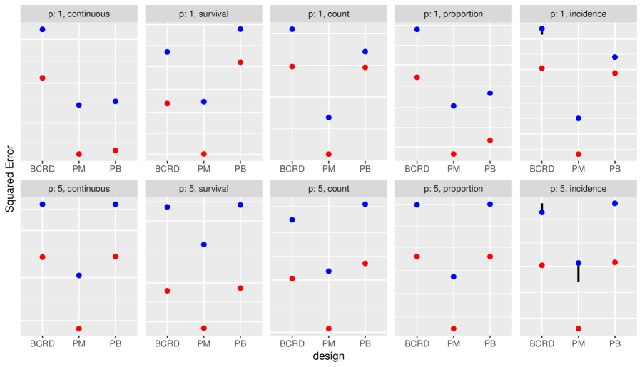
Figure 2: Simulated average MSE (plotted in red) and empirical simultaneous 95%ile MSE tail (plotted in blue) with 95% bootstrap confidence intervals (plotted in black) by design, $n=96$, $p=1,5$, all five investigated response types and all appropriate block sizes. The squared error (the y-axis) is relative to each of the ten individual $p~{}\times$ response type plots and thus its numeric tick labels are unshown.

5 Discussion

Randomized experimentation comes with the choice of “how to randomize”? A default design is complete randomization independent of subjects’ covariates. This is seldom done as the inevitable imbalance among the arms implies a highly visible risk of bias. Can we design one perfect assignment that minimizes covariate imbalance across arms? Although this may “feel” optimal, it is not (except in the case of $p=1$ and a linear response) as the covariate-response models are arbitrarily complicated. Further, this one perfect assignment is NP-hard to compute.

Commonly employed designs are between the two extremes mentioned above; they sacrifice some randomness to get some imbalance reduction. Kapelner et al., (2021) investigated how to harmonize these two considerations for a continuous response to choose a design. Therein we proposed a “single quantile tail criterion” which averages MSE over the design and then takes the quantile of the MSE over unobserved covariate realizations. We showed this a performance metric is a trade-off of both degree of randomness and degree of observed covariate imbalance reduction.

Herein, we propose a more realistic related criterion called the “double quantile tail criterion” which takes the quantile of the MSE over both the experimental allocation and the unobserved covariates for general response types. We then prove that the asymptotically optimal block design is achieved with pairwise matching (PM) and this is our unconditional advice for experimenters. Although this work focuses on estimation, these blocking designs should have high power as well as many allocations can be generated which are highly independent (Krieger et al., , 2020). Additional simulation results (unshown) under larger values of the average treatment effect parameters shows that the design difference performance is especially sensitive to PM versus other blocking designs in cases of small treatment effects; it can make the difference between finding the effect or not.

There are many other avenues to explore. First, although we proved that PM is asymptotically optimal, we did not prove it is uniquely optimal as we only considered block designs. We only proved its optimality for the case of knowing the ordering of the mean response function contributions (a function of the observed covariates and treatment). We would like to prove its optimality under PM in the real-world which uses Mahalanobis-distance matching.

Another area of exploration could be understanding the tail criterion for other designs such as rerandomization and greedy pair switching. Additionally, survival is an important experimental endpoint in clinical trials but this work only considered uncensored survival measurement while the vast majority of survivals collected in real-world experiments are censored. Also, in Kapelner et al., (2021, Section 2.3), we explored the ordinary least squares (OLS) estimator for continuous response. We believe the performance of the OLS estimator in our tail criterion can be analyzed and our intuition is that PM would also emerge as optimal among block designs. However, this avenue would be difficult to explore for general response types as the analogous estimators do not have closed form (e.g. if the response is binary, the multivariate logistic regression estimates are the result of computational iteration). Finally, our tail criterion is only one metric that combines mean and standard deviation of MSE. Other criterions can also be useful such as their ratio (the Sharpe measure). Also, work can be done to find the optimal imbalance design under unequal allocation ($n_{T}\neq n_{C}$). We can also investigate optimal designs for sequential experiments, the most common type of clinical trial.

Funding

This research was supported by Grant No 2018112 from the United States-Israel Binational Science Foundation (BSF).

Supplementary Materials for
“The Pairwise Matching Design is Optimal under Extreme Noise and Assignments”
 
by David Azriel, Abba Krieger and Adam Kapelner

Appendix A Technical Proofs

A.1 Estimator Computation

The contribution to $\hat{\tau}$ from individual $i$ is $\frac{y_{Ti}}{n}$ when $w_{i}=1$ and $-\frac{y_{Ci}}{n}$ when $w_{i}=-1$. This contribution can be summarized as $((y_{Ti}-y_{Ci})+w_{i}(y_{Ti}+y_{Ci}))/(2n)$. When this is summed over all individuals $i$ we have our result

$$\hat{\tau}=\frac{1}{2n}\left(\boldsymbol{1}_{2n}^{\top}\left(\boldsymbol{y}_{T}-\boldsymbol{y}_{C}\right)+\boldsymbol{W}^{\top}\left(\boldsymbol{y}_{T}+\boldsymbol{y}_{C}\right)\right).$$

A.2 Expectation of the MSE

For this section and following sections, let $\boldsymbol{Z}:=\boldsymbol{Z}_{T}+\boldsymbol{Z}_{C}$ and $\boldsymbol{\mu}:=\boldsymbol{\mu}_{T}+\boldsymbol{\mu}_{C}$.

$$= \mathbb{E}_{\,\boldsymbol{Z}_{T},\boldsymbol{Z}_{C}}\left[\mathbb{E}_{\,\boldsymbol{W}}\left[(\hat{\tau}-\tau)^{2}\right]\right]$$

$$= \mathbb{E}_{\,\boldsymbol{Z}_{T},\boldsymbol{Z}_{C}}\left[\frac{1}{4}\left(\frac{\boldsymbol{\mu}_{T}+\boldsymbol{Z}_{T}}{n}+\frac{\boldsymbol{\mu}_{C}+\boldsymbol{Z}_{C}}{n}\right)^{\top}\boldsymbol{\Sigma}_{W}\left(\frac{\boldsymbol{\mu}_{T}+\boldsymbol{Z}_{T}}{n}+\frac{\boldsymbol{\mu}_{C}+\boldsymbol{Z}_{C}}{n}\right)\right]$$

$$= \frac{1}{4n^{2}}\mathbb{E}_{\,\boldsymbol{Z}}\left[\left(\boldsymbol{\mu}+\boldsymbol{Z}\right)^{\top}\boldsymbol{\Sigma}_{W}\left(\boldsymbol{\mu}+\boldsymbol{Z}\right)\right]$$

$$= \frac{1}{4n^{2}}\mathbb{E}_{\,\boldsymbol{Z}}\left[\boldsymbol{\mu}^{\top}\boldsymbol{\Sigma}_{W}\boldsymbol{\mu}+2\boldsymbol{\mu}^{\top}\boldsymbol{\Sigma}_{W}\boldsymbol{Z}+\boldsymbol{Z}^{\top}\boldsymbol{\Sigma}_{W}\boldsymbol{Z}\right]$$

$$= \frac{1}{4n^{2}}\left(\boldsymbol{\mu}^{\top}\boldsymbol{\Sigma}_{W}\boldsymbol{\mu}+\mathbb{E}_{\,\boldsymbol{Z}}\left[\boldsymbol{Z}^{\top}\boldsymbol{\Sigma}_{W}\boldsymbol{Z}\right]\right)$$

$$= \frac{1}{4n^{2}}\left(\boldsymbol{\mu}^{\top}\boldsymbol{\Sigma}_{W}\boldsymbol{\mu}+\text{tr}\left[\boldsymbol{\Sigma}_{W}\boldsymbol{\rho}\right]\right)$$

where $\boldsymbol{\rho}$ denotes the diagonal variance-covariance matrix of $\boldsymbol{Z}$. To compute the trace, we need to consider only the diagonal entries of $\boldsymbol{\Sigma}_{W}\boldsymbol{\rho}$. The $i$th diagonal entry of this product is ${\boldsymbol{\Sigma}_{W}}_{i\,\cdot}{\boldsymbol{\Sigma}_{Z}}_{\cdot\,i}={\boldsymbol{\Sigma}_{W}}_{i\,i}{\boldsymbol{\Sigma}_{Z}}_{i\,i}$ due to $\boldsymbol{\rho}$ being diagonal. From Assumption LABEL:ass:equal_chance_T, we know that all the diagonal entries of $\boldsymbol{\Sigma}_{W}$ are 1 and thus $\text{tr}\left[\boldsymbol{\Sigma}_{W}\boldsymbol{\rho}\right]=\text{tr}\left[\boldsymbol{\rho}\right]$. Upon substitution, the result is

$$\mathbb{E}_{\,\boldsymbol{W},\boldsymbol{Z}_{T},\boldsymbol{Z}_{C}}\left[(\hat{\tau}-\tau)^{2}\right] = \frac{1}{4n^{2}}\left(\boldsymbol{\mu}^{\top}\boldsymbol{\Sigma}_{W}\boldsymbol{\mu}+\text{tr}\left[\boldsymbol{\Sigma}_{W}\boldsymbol{\rho}\right]\right)+\underbrace{\frac{1}{4n^{2}}\text{tr}\left[\boldsymbol{\rho}\right]}.$$

where the underbraced term is design-independent and denoted as $c_{Z}$.

A.3 Proof of Theorem 3.1

By Equation LABEL:eq:estimator, the MSE can be expressed as

$$\text{MSE}:=(\hat{\tau}-\tau)^{2}=\frac{1}{4n^{2}}\left(\boldsymbol{W}^{\top}\left(\boldsymbol{Y}_{T}+\boldsymbol{Y}_{C}\right)\right)^{2}$$

where this notation depresses its dependence on $\boldsymbol{W},\boldsymbol{Z}_{T},\boldsymbol{Z}_{C}$. The variance of the MSE is

$$\mathbb{V}\text{ar}_{\boldsymbol{Z},\boldsymbol{W}}\left[\text{MSE}\right]=\mathbb{V}\text{ar}_{\boldsymbol{Z}}\left[\mathbb{E}_{\,\boldsymbol{W}}\left[\text{MSE}\,|\,\boldsymbol{Z}\right]\right]+\mathbb{E}_{\,\boldsymbol{Z}}\left[\mathbb{V}\text{ar}_{\boldsymbol{W}}\left[\text{MSE}\,|\,\boldsymbol{Z}\right]\right]$$ (4)

where $\boldsymbol{Z}$ denotes the collection of $\boldsymbol{Z}_{T},\boldsymbol{Z}_{C}$.

Proof of part (a)

Consider the variance decomposition in Equation 4. It follows that

$$\mathbb{V}\text{ar}_{\boldsymbol{Z},\boldsymbol{W}_{B}}\left[\text{MSE}\right]\geq\mathbb{E}_{\,\boldsymbol{Z}}\left[\mathbb{V}\text{ar}_{\boldsymbol{W}_{B}}\left[\text{MSE}\,|\,\boldsymbol{Z}\right]\right].$$

Below the latter term is analyzed.

Recall that $\boldsymbol{v}:=\boldsymbol{\mu}+\boldsymbol{Z}$. Consider first the case of $B=n$, i.e., PM. We have that

$$\boldsymbol{v}^{T}\boldsymbol{W}_{n}=U_{1}(v_{2}-v_{1})+U_{2}(v_{4}-v_{3})+\cdots+U_{n}(v_{2n}-v_{2n-1}),$$

where $U_{1},\ldots,U_{n}$ are iid with $P(U=1)=P(U=-1)=1/2$. Since $U_{i}^{2}=1$,

$$4n^{2}\text{MSE}=(\boldsymbol{v}^{T}\boldsymbol{W}_{n})^{2}=\sum_{i=1}^{n}(v_{2i}-v_{2i-1})^{2}+2\sum_{1\leq i<j\leq n}U_{i}U_{j}(v_{2i}-v_{2i-1})(v_{2j}-v_{2j-1})$$

The variance of $U_{i}U_{j}$ for $i\neq j$ is 1 and the covariance between $U_{i}U_{j}$ and $U_{i^{\prime}}U_{j^{\prime}}$ is 0 if $(i,j)\neq(i^{\prime},j^{\prime})$, $i<j,i^{\prime}<j^{\prime}$; therefore,

$$\mathbb{V}\text{ar}_{\boldsymbol{W}_{n}}\left[\text{MSE}\,|\,\boldsymbol{Z}\right]=\frac{1}{16n^{4}}\sum_{1\leq i<j\leq n}(v_{2i}-v_{2i-1})^{2}(v_{2j}-v_{2j-1})^{2}.$$ (5)

Thus,

$$\mathbb{E}_{\,\boldsymbol{Z}}\left[\mathbb{V}\text{ar}_{\boldsymbol{W}_{n}}\left[\text{MSE}\,|\,\boldsymbol{Z}\right]\right]\\ =\frac{1}{16n^{4}}\sum_{1\leq i<j\leq n}[(\mu_{2i}-\mu_{2i-1})^{2}(\mu_{2j}-\mu_{2j-1})^{2}+(\mu_{2i}-\mu_{2i-1})^{2}(\rho_{2j}+\rho_{2j-1})+(\mu_{2j}-\mu_{2j-1})^{2}(\rho_{2i}+\rho_{2i-1})]\\ +\frac{1}{16n^{4}}\sum_{1\leq i<j\leq n}(\rho_{2i}+\rho_{2i-1})(\rho_{2j}+\rho_{2j-1}).$$ (6)

Hence,

$$\mathbb{E}_{\,\boldsymbol{Z}}\left[\mathbb{V}\text{ar}_{\boldsymbol{W}_{n}}\left[\text{MSE}\,|\,\boldsymbol{Z}\right]\right]\geq\frac{1}{16n^{4}}\sum_{1\leq i<j\leq n}(\rho_{2i}+\rho_{2i-1})(\rho_{2j}+\rho_{2j-1})\\ =\frac{1}{32n^{4}}\sum_{i,j\in\{1,\ldots,n\}}(\rho_{2i}+\rho_{2i-1})(\rho_{2j}+\rho_{2j-1})+O(1/n^{3})=\frac{1}{32n^{4}}(\boldsymbol{1}_{2n}^{\top}\boldsymbol{\rho})^{2}+O(1/n^{3})=\frac{\bar{\rho}^{2}}{8n^{2}}+o(1/n^{2}).$$ (7)

Consider now a block design with $B$ blocks and recall that $\boldsymbol{W}_{B}$ is a random allocation from this design. The vector $\boldsymbol{W}_{B}$ can be thought of as a mixture over pairwise designs in the following way. Let $2n_{B}$ be the number of subjects in each block. Let $P_{b}$ be a random partition of the $2n_{B}$ subjects into $n_{B}$ pairs for block $b$. A random partition is then $P_{J}:=P_{1}\times P_{2}\times\ldots\times P_{B}$. Each random partition produces $n$ pairwise matches. Then

$$\mathbb{V}\text{ar}_{\boldsymbol{W}_{B}}\left[\text{MSE}\,|\,\boldsymbol{Z}\right] =\mathbb{E}_{\,P_{J}}\left[\mathbb{V}\text{ar}_{\boldsymbol{W}_{B}}\left[\text{MSE}\,|\,\boldsymbol{Z},P_{J}\right]\,|\,\boldsymbol{Z}\right]+\mathbb{V}\text{ar}_{P_{J}}\left[\mathbb{E}_{\,\boldsymbol{W}_{B}}\left[\text{MSE}\,|\,\boldsymbol{Z},P_{J}\right]\,|\,\boldsymbol{Z}\right]$$

$$\geq\mathbb{E}_{\,P_{j}}\left[\mathbb{V}\text{ar}_{\boldsymbol{W}_{B}}\left[\text{MSE}\,|\,\boldsymbol{Z},P_{J}\right]\,|\,\boldsymbol{Z}\right]$$

and therefore,

$$\mathbb{E}_{\,Z}\left[\mathbb{V}\text{ar}_{\boldsymbol{W}_{B}}\left[\text{MSE}\,|\,\boldsymbol{Z}\right]\right]\geq\mathbb{E}_{\,Z}\left[\mathbb{E}_{\,P_{J}}\left[\mathbb{V}\text{ar}_{\boldsymbol{W}_{B}}\left[\text{MSE}\,|\,\boldsymbol{Z},P_{J}\right]\,|\,\boldsymbol{Z}\right]\right]=\mathbb{E}_{\,Z,P_{J}}\left[\mathbb{V}\text{ar}_{\boldsymbol{W}_{B}}\left[\text{MSE}\,|\,\boldsymbol{Z},P_{J}\right]\right].$$

Since given $P_{J}$, $\boldsymbol{W}_{B}$ is a PM design, Equation 7 implies that for every $P_{J}$

$$\mathbb{E}_{\,Z}\left[\mathbb{V}\text{ar}_{\boldsymbol{W}_{B}}\left[\text{MSE}\,|\,\boldsymbol{Z},P_{J}\right]\,|\,P_{J}\right]\geq\frac{\bar{\rho}^{2}}{8n^{2}}+o(1/n^{2}),$$

which completes the proof of the part (a) because

$$\mathbb{E}_{\,P_{J}}\left[\mathbb{E}_{\,Z}\left[\mathbb{V}\text{ar}_{\boldsymbol{W}_{B}}\left[\text{MSE}\,|\,\boldsymbol{Z},P_{J}\right]\,|\,P_{J}\right]\right]=\mathbb{E}_{\,Z,P_{J}}\left[\mathbb{V}\text{ar}_{\boldsymbol{W}_{B}}\left[\text{MSE}\,|\,\boldsymbol{Z},P_{J}\right]\right].$$

Proof of part (b)

Consider the variance decomposition in Equation 4. Theorem 3.4 of our previous paper implies that if the fourth moment of $Z_{i}$ is bounded (Assumption 3.1) then for PM

$$\mathbb{V}\text{ar}_{\boldsymbol{Z}}\left[\mathbb{E}_{\,\boldsymbol{W}_{n}}\left[\text{MSE}\,|\,\boldsymbol{Z}\right]\right]=O(1/n^{3}).$$

Hence, when multiplying by $n^{2}$ this term vanishes.

Consider now $\mathbb{E}_{\,\boldsymbol{Z}}\left[\mathbb{V}\text{ar}_{\boldsymbol{W}_{n}}\left[\text{MSE}\,|\,\boldsymbol{Z}\right]\right]$. By Equation 6,

$$n^{2}\mathbb{E}_{\,\boldsymbol{Z}}\left[\mathbb{V}\text{ar}_{\boldsymbol{W}_{n}}\left[\text{MSE}\,|\,\boldsymbol{Z}\right]\right] = \frac{1}{16n^{2}}\sum_{1\leq i<j\leq n}(\mu_{2i}-\mu_{2i-1})^{2}(\mu_{2j}-\mu_{2j-1})^{2}+$$ (10)

$$\frac{n-1}{8n^{2}}\sum_{i=1}^{n}(\mu_{2i}-\mu_{2i-1})^{2}(\rho_{2i}+\rho_{2i-1})+$$

$$\frac{1}{16n^{2}}\sum_{1\leq i<j\leq n}(\rho_{2i}+\rho_{2i-1})(\rho_{2j}+\rho_{2j-1}).$$

The term in Equation 10 vanishes asymptotically because

$$\frac{1}{n^{2}}\sum_{1\leq i<j\leq n}(\mu_{2i}-\mu_{2i-1})^{2}(\mu_{2j}-\mu_{2j-1})^{2} \leq\frac{2}{n^{2}}\sum_{i=1}^{n}\sum_{j=1}^{n}(\mu_{2i}-\mu_{2i-1})^{2}(\mu_{2j}-\mu_{2j-1})^{2}$$

$$=2\left(\frac{1}{n}\sum_{i=1}^{n}(\mu_{2i}-\mu_{2i-1})^{2}\right)^{2}$$

which goes to 0 by the assumption that $\frac{1}{n}\sum_{i=1}^{n}(\mu_{2i}-\mu_{2i-1})^{2}\to 0$. The term in Equation 10 vanishes because we assumed that $\frac{1}{n}\sum_{i=1}^{n}(\mu_{2i}-\mu_{2i-1})^{2}\to 0$ and that the $\rho$’s are bounded. Thus, the dominant term is in Equation 10, and it is equal to

$$\footnotesize\frac{1}{16n^{2}}\sum_{1\leq i<j\leq n}(\rho_{2i}+\rho_{2i-1})(\rho_{2j}+\rho_{2j-1}) = \frac{1}{32n^{2}}\sum_{i,j\in\{1,\ldots,n\}}(\rho_{2i}+\rho_{2i-1})(\rho_{2j}+\rho_{2j-1})+O\left(n^{-1}\right)$$

$$= \frac{1}{8}\left(\frac{1}{2n}\sum_{i=1}^{2n}\rho_{i}\right)^{2}+O\left(n^{-1}\right)$$

$$= \frac{\bar{\rho}^{2}}{8}+o(1),$$

thereby completing the proof. ∎

A.4 The variance of the MSE under PB

Consider $\boldsymbol{w}_{*}$ and its mirror $-\boldsymbol{w}_{*}$, vectors that both uniquely minimize $|(\boldsymbol{\mu}_{T}+\boldsymbol{\mu}_{C})^{\top}\boldsymbol{w}|$. The PB design is composed of the random variable $\boldsymbol{W}$ that draws $\boldsymbol{w}_{*}$ and $-\boldsymbol{w}_{*}$ each with probability 1/2. Thus, conditional on $\boldsymbol{Z}$,

$$\text{MSE}:=(\hat{\tau}-\tau)^{2}=\frac{1}{4n^{2}}\left(\boldsymbol{W}^{\top}\left(\boldsymbol{Y}_{T}+\boldsymbol{Y}_{C}\right)\right)^{2}$$

is constant implying that $\mathbb{V}\text{ar}_{\boldsymbol{W}}\left[\text{MSE}\,|\,\boldsymbol{Z}\right]=0$. The decomposition of the variance of the MSE (Equation 4) is thus only

$$\mathbb{V}\text{ar}_{\boldsymbol{Z},\boldsymbol{W}}\left[\text{MSE}\right]=\mathbb{V}\text{ar}_{\boldsymbol{Z}}\left[\mathbb{E}_{\,\boldsymbol{W}}\left[\text{MSE}\,|\,\boldsymbol{Z}\right]\right].$$

This expression was computed in Sections 3.3.3 and A.9 of Azriel et al., (2023) where it was shown that under Assumptions 3.1, 3.2 and 3.3,

$$\mathbb{V}\text{ar}_{\boldsymbol{Z}}\left[\mathbb{E}_{\,\boldsymbol{W}}\left[\text{MSE}\,|\,\boldsymbol{Z}\right]\right]=\frac{1}{16n^{4}}\left(O(n)+2\left(\sum_{i=1}^{2n}\rho_{i}\right)^{2}\right)=\frac{1}{16n^{4}}\left(O(n)+8n^{2}\left(\bar{\rho}^{2}\right)\right).$$

It follows that under PB,

$$\lim_{n\to\infty}n^{2}\,\mathbb{V}\text{ar}_{\boldsymbol{W}_{n},\boldsymbol{Z}_{T},\boldsymbol{Z}_{C}}\left[(\hat{\tau}-\tau)^{2}\right]=\frac{\bar{\rho}^{2}}{2}.$$

References

- Azriel et al., (2023) Azriel, D., Krieger, A. M., and Kapelner, A. (2023). The optimality of blocking designs in equally and unequally allocated randomized experiments with general response. arXiv (2212.01887).
- Beck et al., (2016) Beck, C., Lu, B., and Greevy, R. (2016). nbpmatching: Functions for optimal non-bipartite matching. r package version 1.5.1.
- Fisher, (1925) Fisher, R. A. (1925). Statistical methods for research workers. Edinburgh Oliver & Boyd.
- Freedman, (2008) Freedman, D. A. (2008). On regression adjustments to experimental data. Advances in Applied Mathematics, 40(2):180–193.
- Greevy et al., (2004) Greevy, R., Lu, B., Silber, J. H., and Rosenbaum, P. (2004). Optimal multivariate matching before randomization. Biostatistics, 5(2):263–275.
- Harville, (1975) Harville, D. A. (1975). Experimental randomization: Who needs it? The American Statistician, 29(1):27–31.
- Kallus, (2018) Kallus, N. (2018). Optimal a priori balance in the design of controlled experiments. Journal of the Royal Statistical Society: Series B (Statistical Methodology), 80(1):85–112.
- Kapelner et al., (2021) Kapelner, A., Krieger, A. M., Sklar, M., Shalit, U., and Azriel, D. (2021). Harmonizing optimized designs with classic randomization in experiments. The American Statistician, 75(2):195–206.
- Kiefer and Wolfowitz, (1959) Kiefer, J. and Wolfowitz, J. (1959). Optimum designs in regression problems. The Annals of Mathematical Statistics, pages 271–294.
- Krieger et al., (2019) Krieger, A. M., Azriel, D., and Kapelner, A. (2019). Nearly random designs with greatly improved balance. Biometrika, 106(3):695–701.
- Krieger et al., (2020) Krieger, A. M., Azriel, D., Sklar, M., and Kapelner, A. (2020). Improving the power of the randomization test. arXiv preprint arXiv:2008.05980.
- Li et al., (2018) Li, X., Ding, P., and Rubin, D. B. (2018). Asymptotic theory of rerandomization in treatment–control experiments. Proceedings of the National Academy of Sciences, 115(37):9157–9162.
- Lin, (2013) Lin, W. (2013). Agnostic notes on regression adjustments to experimental data: Reexamining freedman’s critique. The Annals of Applied Statistics, 7(1):295–318.
- Lu et al., (2011) Lu, B., Greevy, R., Xu, X., and Beck, C. (2011). Optimal nonbipartite matching and its statistical applications. The American Statistician, 65(1):21–30.
- Morgan and Rubin, (2012) Morgan, K. L. and Rubin, D. B. (2012). Rerandomization to improve covariate balance in experiments. The Annals of Statistics, pages 1263–1282.
- Rosenberger and Lachin, (2016) Rosenberger, W. F. and Lachin, J. M. (2016). Randomization in clinical trials: theory and practice. John Wiley & Sons, second edition.
- Rubin, (2005) Rubin, D. B. (2005). Causal inference using potential outcomes: Design, modeling, decisions. Journal of the American Statistical Association, 100(469):322–331.
- Senn, (2013) Senn, S. (2013). Seven myths of randomisation in clinical trials. Statistics in Medicine, 32(9):1439–1450.
- Smith, (1918) Smith, K. (1918). On the standard deviations of adjusted and interpolated values of an observed polynomial function and its constants and the guidance they give towards a proper choice of the distribution of observations. Biometrika, 12(1/2):1–85.
- Steinberg and Hunter, (1984) Steinberg, D. M. and Hunter, W. G. (1984). Experimental design: review and comment. Technometrics, 26(2):71–97.
- Stuart, (2010) Stuart, E. A. (2010). Matching methods for causal inference: A review and a look forward. Statistical science, 25(1):1.
- Student, (1938) Student (1938). Comparison between balanced and random arrangements of field plots. Biometrika, pages 363–378.
- Teugels, (1990) Teugels, J. L. (1990). Some representations of the multivariate bernoulli and binomial distributions. Journal of multivariate analysis, 32(2):256–268.
- Wu, (1981) Wu, C. F. (1981). On the robustness and efficiency of some randomized designs. The Annals of Statistics, pages 1168–1177.