Thresholded Oja does Sparse PCA?

Abstract

We consider the problem of Sparse Principal Component Analysis (PCA) when the ratio $d/n\rightarrow c>0$. There has been a lot of work on optimal rates on sparse PCA in the offline setting, where all the data is available for multiple passes. In contrast, when the population eigenvector is $s$-sparse, streaming algorithms that have $O(d)$ storage and $O(nd)$ time complexity either typically require strong initialization conditions or have a suboptimal error. We show that a simple algorithm that thresholds and renormalizes the output of Oja’s algorithm (the Oja vector) obtains a near-optimal error rate. This is very surprising because, without thresholding, the Oja vector has a large error. Our analysis centers around bounding the entries of the unnormalized Oja vector, which involves the projection of a product of independent random matrices on a random initial vector. This is nontrivial and novel since previous analyses of Oja’s algorithm and matrix products have been done when the trace of the population covariance matrix is bounded while in our setting, this quantity can be as large as $n$.

1 Introduction

Principal Component Analysis (PCA) [40, 24] is a classic method for data analysis and visualization. It has gained popularity due to its simplicity and effectiveness in extracting meaningful information from complex datasets. Given a dataset $\left\{X_{i}\right\}_{i=1,\dots,n}$ where $X_{i}\in\mathbb{R}^{d}$, sampled independently from a distribution with mean zero and covariance matrix $\Sigma$, PCA aims to find orthogonal directions that capture most of the variance. As a first step, we will examine the foundational problem of finding an estimate of $v_{1}$, the leading eigenvector of $\Sigma$, as:

$$\widehat{v}:=\operatorname*{arg\,max}_{w\in\mathbb{R}^{d}}\left(X_{i}^{T}w\right)^{2},\text{ s.t.}\left\lVert w\right\rVert_{2}=1$$ (1)

For the classical statistical setting where $d$ is fixed, and $n$ goes to infinity, the most natural estimator is to return the first eigenvector of the sample covariance matrix $\hat{\Sigma}=\sum_{i}X_{i}X_{i}^{T}/n$. It is well known that under suitable tail conditions, $\|\hat{\Sigma}-\Sigma\|=O\left(\sqrt{r_{\text{eff}}/n}\right)$ with high probability (see Theorem 9.2.4 in [45]) where $r_{\text{eff}}:=\frac{\operatorname{Tr}\left(\Sigma\right)}{\left\lVert\Sigma\right\rVert}$ is the effective rank. Thus, if $\operatorname{Tr}(\Sigma)$ grows slowly with $n$, which is true when $d/n\rightarrow 0$, we have consistency. The consistency of the principal eigenvector of the empirical covariance matrix results from a straightforward application of Wedin’s theorem [50, 20].

Another classical and perhaps more computational question is how to estimate principal component(s) in the streaming setting. Here, data points arrive one at a time, sampled from a suitable distribution independently, and one is only allowed $O(d)$ storage. Streaming algorithms typically perform a single pass over the dataset and maintain an online estimate. This setting is particularly attractive due to its computational and space efficiency. In a streaming context, solving Eq 2 traces back to Canadian psychologist Donald Hebb’s research [13], which was later formalized in the seminal work of Erkki Oja [37]. The main idea in Oja’s algorithm is a simple projected stochastic gradient descent algorithm, which has been analyzed in theoretical Statistics and Computer Science communities in great detail [20, 1, 7, 52, 14, 18, 35, 29, 34, 19]. Notably, [20], [1], and [18] establish that Oja’s algorithm achieves a similar error as the offline algorithm that estimates the top eigenvector of the empirical covariance matrix. Not surprisingly, the $\sin^{2}$ error (Eq 3) between $v_{1}$ and the estimate (call this the Oja vector) goes to zero as $r_{\text{eff}}/n$ similar to the error of the principal eigenvector of the $\hat{\Sigma}$.

In the streaming context, the regime where $r_{\text{eff}}$ is comparable to $n$, has not received a lot of attention. In contrast, in the offline setting there has been a myriad of important results showing the inconsistency of PCA [39, 26, 23].The existing work on high-dimensional PCA or covariance estimation operates under some additional structural assumptions on $\Sigma$ or $v_{1}$. In many practical scenarios, $v_{1}$ satisfies additional structure, which can be exploited to obtain better estimators. Sparse PCA is one of the most widely studied classes of such problems, where $v_{1}$ is assumed to have only $s$ non-zero components, where $s<d$. Sparsity enhances interpretability and provides variable selection along with PCA. Formally, Sparse PCA can be framed as the optimization problem:

$$\widehat{v}_{\text{sparse}}:=\operatorname*{arg\,max}_{w\in\mathbb{R}^{d}}\left(X_{i}^{T}w\right)^{2},\text{ under constraints }\left\lVert w\right\rVert_{2}=1,\;\left\lVert w\right\rVert_{0}\leq s$$ (2)

where $\left\lVert.\right\rVert_{0}$ denotes the $l_{0}$ norm, i.e., the number of non-zero entries of the vector. We refer to such a $w$ as being $s$-sparse. The optimization problem in Eq (2) is non-convex and is also NP-hard [33] since it can be reduced to subset selection for ordinary least squares regression. Therefore, several approximation algorithms have been proposed in the literature.

[46, 6] showed a $O\left(s\log\left(d\right)/n\right)$ minimax lower bound for the statistical estimation error (Def. 3) of $\widehat{v}$, therefore setting a baseline. There are many sophisticated and optimal offline algorithms for sparse PCA. Some are convex relaxation based [3, 8, 47, 44, 55, 10, 2, 30, 6]. Some involve iterated thresholding [25, 30, 54] where a variant of the power-method is analyzed along with thresholding to achieve sparsity.

Most SDP-based algorithms such as  [2, 47, 8] do not scale well in high-dimensions, as mentioned in  [3, 48]. The state-of-the-art SDP solvers [22, 16] currently have a runtime $\Omega\left(n^{\omega}+d^{\omega}\right)$, where $\omega\approx 2.732$ is the matrix multiplication exponent. Algorithms proposed in [30, 6, 54, 25] involve forming the entire $\left(d\times d\right)$ sample covariance matrix, which can itself be challenging from the perspective of space and time complexity in high dimensions. Furthermore, [30, 6] have been analyzed under the spiked covariance model, which places specific structural assumptions on the covariance matrix. Iterated thresholding algorithms such as [54] provide convergence guarantees under a strong initialization condition of the starting iterate. These enhance the appeal of streaming algorithms with an easy initialization procedure that process one data point at a time and operate in $O\left(nd\right)$ time, $O\left(d\right)$ space. However, in the high-dimensional context, the streaming PCA problem has received limited attention.  [53, 49] provide streaming sparse PCA algorithms for the spiked-covariance model (where the covariance matrix is a sum of a low-rank matrix with structural assumptions and a scalar multiple of identity).  [53] provide an algorithm which is an online block version of the truncated power method in [54]. However, they require an initial estimate of the vector with a sufficiently large inner product with the true $v_{1}$ (similar to [54]). Their proposed initialization method also relies on an initialization using a streaming PCA algorithm until reaching a specific accuracy threshold. There is no known theoretical guarantee of why this threshold will be achieved in the spiked high-dimensional setting.  [49] provides an analysis of scaling in high dimensions via partial differential equations (PDE), but they only prove convergence, not explicit error guarantees.  [42] propose a computationally efficient modification of the Fantope projection-based algorithm of [47] along with an online variant. As noted by them, the online version of their algorithm is the first to provably obtain the global optima in a streaming setting without any initialization. However, the estimation error bound achieved by their algorithm is $O\left(1/\sqrt{n}\right)$ (Theorem 4, [42]), which has suboptimal dependence on $n$. Table 1 presents a detailed comparison of the algorithms discussed in this paragraph for Sparse PCA (Eq 2) based on various relevant parameters discussed above.

Paper(s)	Storage	Time	Initialization?	Spiked Model?	$\sin^{2}$ error
Yang and Xu [53]	$O\left(d\right)$	$O\left(nd\right)$	Y	Y	$O\left(\frac{s\log\left(d\right)}{n}\right)$
Wang and Lu [49]	$O\left(d\right)$	$O\left(nd\right)$	Y	Y	$-$
Qiu et. al [42] (Thm. 4)	$O\left(d\right)$	$O\left(nd\right)$	N	N	$O\left(\frac{1}{\sqrt{n}}\right)$
Theorem 1	$O\left(d\right)$	$O\left(nd\right)$	N	N	$O\left(\frac{s\log\left(d\right)}{n}\right)$

Table 1: Comparison of streaming sparse PCA algorithms for extracting the leading eigenvector, based on various parameters, under $\frac{d}{n}\rightarrow c,c>0$. We record the space and time complexity of the algorithm along with whether it is streaming, requires a strong initialization, and if the guarantees are only proven for a spiked covariance model. For [54], the error guarantees are provided for the case of the spiked model for comparison with other results, under the initialization conditions required by Thm. 4 in their paper. We point out that the results of  [54, 53, 49, 42] may be valid in other regimes of the ratio, $\frac{d}{n}$. Note that Theorem 2 also achieves the same guarantees as Theorem 1 on all parameters.

In an attempt to understand the gap between streaming and offline PCA problems in high dimension, we ask a simple question:

When $v_{1}$ is $s-$sparse and the effective rank is comparable to $n$, is there a streaming algorithm that achieves the $\sin^{2}$ error, i.e. $1-\langle\widehat{v},v_{1}\rangle^{2}$ of $O\left(\dfrac{s\log d}{n}\right)$ with $O(d)$ space and $O(nd)$ time complexity?

We provide a surprisingly simple answer. If we simply threshold and renormalize the Oja vector, then in the aforementioned regime, it achieves a $O\left(\dfrac{s\log d}{n}\right)$ $\sin^{2}$ error rate (see Definition 3).

In the offline setting, there has been a similar attempt by [43], who show that the eigenvector of the covariance matrix can be thresholded to obtain the support when $n$ is fixed, $d$ and $\lambda_{1}=d^{\alpha}\rightarrow\infty$. Surprisingly enough, in the streaming context, this has not been studied. Note that we cannot expect the effective rank $r$ to exceed $n$. To see this, take the simple spiked covariance model where $\Sigma=\nu v_{1}v_{1}^{T}+I_{d}$. Assume $d/n\rightarrow c$.  [23] show that $\langle\hat{v},v_{1}\rangle^{2}\rightarrow\frac{(\nu^{2}-c)_{+}}{\nu^{2}+c\nu}.$ The Oja vector, in adversarial settings, has been shown to be aligned with the principal eigenvector ($\hat{v}$) of the empirical covariance matrix [41]. $\hat{v}$ is nearly orthogonal to $v_{1}$, which happens if $c>\nu^{2}$. When $\nu=\widetilde{\Omega}(1)$ the $\sin^{2}$ error is $O(1/\nu)$, far from $O\left(s\log d/n\right)$.

In this paper, we show the surprising result that when $r=\alpha n$ (for some constant $\alpha<1$), and $\nu=\widetilde{\Omega}(1)$, a simple algorithm that hard thresholds by keeping top $s$ elements of the Oja vector and renormalizing it, obtains a $O\left(s\log d/n\right)$ rate of error. Our analysis is highly nontrivial since most results with optimal rates for streaming PCA assume that the vectors, though potentially high-dimensional, are bounded a.s. These results typically involve concentration inequalities of products of bounded random matrices [17, 15]. The bounded assumption was replaced by others [29, 28] by boundedness (or slow growth) assumptions on the moments of suitable quantities. So, we cannot rely on the techniques they developed. Neither can we use techniques for high-dimensional covariance matrix thresholding type arguments in [4, 43, 48] because we deal with matrix products. We use a novel analysis of entrywise analysis of the Oja vector in this high-dimensional setting. In contrast to existing streaming sparse PCA algorithms, we do not require a good initialization. We tease out the fact that, while nothing concentrates around their expectation, the elements of the unnormalized Oja vector in the support of $v_{1}$ are much larger compared to those outside.

Here is a rough outline of our paper. We start with describing the problem setup and assumptions in Section 2. Then we present our main results in Section 3 along with important building blocks in Sections 3.1 and 3.2. Finally, we provide a sketch of the proof along with the techniques used in Section 4.

2 Problem Setup and Preliminaries

Notation. $\mathbb{E}\left[.\right]$ denotes the expectation operator. We use $[n]$ to denote $\{1,\dots,n\}$. Statistical independence between random variables $X$ and $Y$ is represented as $X\perp\!\!\!\perp Y$. $\left\lVert.\right\rVert_{2}$ denotes the $l^{2}$ norm for vectors, and the operator norm for matrices, $\left\lVert.\right\rVert_{F}$ denotes the Frobenius norm and $\left\lVert.\right\rVert_{0}$ denotes the $l^{0}$ norm for vectors and is given as the number of non-zero entries in the vector. For $v\in\mathbb{R}^{d}$, we define $u:=\left\lfloor v\right\rfloor_{R},u\in\mathbb{R}^{d}$ as the truncated vector formed by keeping entries of $v$ in the set $R$ and setting the remaining entries to 0 and $|v|$ as the vector formed by taking an entry-wise absolute value of the elements of $v$. For positive semidefinite matrix $M\in\mathbb{R}^{d\times d}$, we define the norm $\left\lVert v\right\rVert_{M}=\left\lVert M^{\frac{1}{2}}v\right\rVert_{2}$. Let $I\equiv I_{d}\in\mathbb{R}^{d\times d}$ be the $\left(d\times d\right)$ identity matrix and let $e_{i}\in\mathbb{R}^{d\times 1}$ denote the $i^{th}$ column of $I$. For any set $T\subseteq[d]$, we define $I_{T}\in\mathbb{R}^{d\times d}$ as $I_{T}\left(i,j\right)=\mathbbm{1}(i,j\in T)\mathbbm{1}(i=j)$, where $\mathbbm{1}\left(\mathcal{E}\right)$ denotes the indicator random variable corresponding to the event $\mathcal{E}$. We will also use $\langle A,B\rangle:=\operatorname{Tr}(A^{T}B)$ for two matrices $A$ and $B$ with the same dimensions. We will use $\widetilde{O}$ and $\widetilde{\Omega}$ as standard order notations with logarithmic factors.

Definition 2.1.

(Subgaussianity) A random mean-zero vector $X\in\mathbb{R}^{d}$ with covariance matrix $\Sigma$ is a $\sigma-$subgaussian random vector ($\sigma>0$) if for all vectors $v\in\mathbb{R}^{d}$, we have $\mathbb{E}\left[\exp\left(v^{T}X\right)\right]\leq\exp\left(\left\lVert v\right\rVert_{\Sigma}^{2}\sigma^{2}/2\right)$. Equivalently, $\exists\;L>0$, such that $\forall p\geq 2$, $\left(\mathbb{E}\left[|v^{T}X|^{p}\right]\right)^{\frac{1}{p}}\leq L\sigma\sqrt{p}\left\lVert v\right\rVert_{\Sigma}$.

This definition of subgaussianity has been used in contemporary works on PCA and covariance estimation (See for example [32, 21, 11] and Theorem 4.7.1 in [45]).

Data. Let $X_{1},X_{2},\cdots X_{n}$ be a sample of independent and identically distributed $\sigma$-subgaussian vectors in $\mathbb{R}^{d}$ with covariance matrix $\Sigma:=\mathbb{E}\left[X_{i}X_{i}^{T}\right]$. We denote the eigenvectors of $\Sigma$ as $v_{1},v_{2},\cdots v_{d}$ and the corresponding eigenvalues as $\lambda_{1}>\lambda_{2}\geq\cdots\lambda_{d}$. Define $V_{\perp}:=\left[v_{2},v_{3},\cdots v_{d}\right]\in\mathbb{R}^{d\times\left(d-1\right)}$ and $\Lambda_{2}\in\mathbb{R}^{\left(d-1\right)\times\left(d-1\right)}=\operatorname{diag}\left(\lambda_{2},\lambda_{3},\cdots\lambda_{d}\right)$.

Assumption 2 (High-dimensional regime).

We assume $d=cn$, $\frac{\operatorname{Tr}\left(\Sigma\right)}{\lambda_{1}}\leq\alpha n$ for some model dependent parameter $\alpha<1$. We further assume a sufficient spectral gap, $\frac{\lambda_{1}}{\lambda_{2}}\geq\widetilde{\Omega}\left(1\right)$, where $\widetilde{\Omega}\left(.\right)$ hides logarithmic factors in $d$ and constants depending on model parameters.

Objective. Our goal is to estimate the leading eigenvector $v_{1}$ in an online manner, given the dataset $X_{1},\cdots X_{n}$. We work under the following sparsity assumption:

Assumption 3 (Sparsity).

The leading eigenvector, $v_{1}$, is $s$-sparse, i.e $\left\lVert v\right\rVert_{0}\leq s$ for $s=o\left(\frac{d}{\log\left(d\right)}\right)$. The support of $v_{1}$ is denoted as $S:=\left\{i:v_{1}\left(i\right)\neq 0\right\}$.

Error metric. Let the estimate of $v_{1}$ be given as $\widehat{v}$. Then, convergence is measured with respect to the $\sin^{2}$ error given as -

$$\sin^{2}\left(\widehat{v},v_{1}\right):=1-\left(\widehat{v}^{T}v_{1}\right)^{2}=\frac{1}{2}\left\lVert v_{1}v_{1}^{T}-\widehat{v}\widehat{v}^{T}\right\rVert_{F}^{2}$$ (3)

We define $S_{\text{hi}}:=\left\{i:i\in S,\;|v_{1}\left(i\right)|\geq\sqrt{\frac{\log\left(d\right)}{n}}\right\},\;s^{\prime}:=|S_{\text{hi}}|\leq s$. $S_{\text{hi}}$ represents the set of elements in $S$ that are large. Intuitively, when trying to approximate the sparse vector $v_{1}$ for the $\sin^{2}$ error metric through our Algorithms, we only argue about whether $S_{\text{hi}}\subseteq\widehat{S}$, for $\widehat{S}$ returned by the algorithm. The definition of $S_{\text{hi}}$ ensures that the error contribution of the excluded entries is small.

Oja’s Algorithm. Here we describe Oja’s algorithm [38] with a constant learning rate $\eta$ and initial vector $z_{0}$. We will denote this by $\mathsf{Oja}\left(\left\{X_{i}\right\}_{i\in[n]},\eta,z_{0}\right)$. Given an initial vector $z_{0}$, it simply updates $z_{t}\leftarrow(I+\eta X_{t}X_{t}^{T})z_{t-1}$ for every datapoint $X_{t}$. This is followed by normalization $z_{t}\leftarrow\frac{z_{t}}{\|z_{t}\|_{2}}$. This is used as a subroutine in our subsequent results (Algorithms  1 and  2). For convenience of analysis, we define $\forall t\in[n]$,

$$B_{t}:=\left(I+\eta X_{t}X_{t}^{T}\right)\left(I+\eta X_{t-1}X_{t-1}^{T}\right)\cdots\left(I+\eta X_{1}X_{1}^{T}\right),B_{0}=I$$ (4)

From now on, we operate under Assumptions 2 and 3 unless otherwise specified.

3 Main Results

Our method is described in Algorithm 1. It takes as input the dataset $\left\{X_{i}\right\}_{i\in[n]}$, the learning rate $\eta$ and a truncation parameter $k$, which denotes the desired sparsity level. When given a dataset $\left\{X_{i}\right\}_{i\in[n]}$, we split the dataset into two parts of equal size. Using the first half set of samples, we estimate the support set $\widehat{S}$, and using the second half of samples we estimate $v_{1}$. Both procedures use Oja’s Algorithm as a subroutine. We analyze two natural ideas for support recovery - A cardinality-based truncation method in Algorithm 1, and a value-based truncation method in Algorithm 2 (Section A.4.1 of the Appendix).

Algorithm 1 $\mathsf{Oja}$-$\mathsf{Top}$-$\mathsf{k}\left(\left\{X_{i}\right\}_{i\in[n]},k,\eta\right)$

1:  Input : Dataset $\left\{X_{i}\right\}_{i\in[n]}$, learning rate $\eta>0$, Cardinality parameter $k\geq s$

2:  $w_{0},y_{0}\sim\mathcal{N}\left(0,I\right)$

3:  $\hat{v}_{1}\leftarrow\mathsf{Oja}\left(\left\{X_{i}\right\}_{i\in[n/2]},\eta,y_{0}\right)$

4:  $\hat{v}_{2}\leftarrow\mathsf{Oja}\left(\left\{X_{i}\right\}_{i\in\{n/2+1,\dots,n\}},\eta,w_{0}\right)$

5:  $\widehat{S}\leftarrow\text{ Indices of }k\text{ largest values of}\left|\hat{v}_{1}\right|$

6:  $\hat{v}_{\text{oja-top-k}}\leftarrow\frac{\left\lfloor\widehat{v}_{2}\right\rfloor_{\widehat{S}}}{\left\lVert\left\lfloor\widehat{v}_{2}\right\rfloor_{\widehat{S}}\right\rVert_{2}}$

7:  return  $\left[\hat{v}_{\text{oja-top-k}},\widehat{S}\right]$

[Convergence of $\mathsf{Oja}$-$\mathsf{Top}$-$\mathsf{k}$] Let $\hat{v}_{\text{oja-top-k}},\;\;\widehat{S}$ be obtained from Algorithm 1. Set the learning rate as $\eta:=\frac{3\log\left(n\right)}{{n\left(\lambda_{1}-\lambda_{2}\right)}}$. Then, for $n=\widetilde{\Omega}\left(\frac{1}{\min_{i\in S_{\text{hi}}}v_{1}\left(i\right)^{2}}\frac{\lambda_{1}}{\lambda_{1}-\lambda_{2}}\right)^{2}$, with probability at least $3/4$, we have, for absolute constant $C^{\prime\prime}>0$,

$$\sin^{2}\left(\hat{v}_{\text{oja-top-k}},v_{1}\right)\leq C^{\prime\prime}\left(\frac{\lambda_{1}}{\lambda_{1}-\lambda_{2}}\right)^{2}\frac{k\log\left(n\right)}{n},\;\text{ and}\;S_{\text{hi}}\subseteq\widehat{S},$$

The error rate in Theorem 1 is optimal in its dependence on $s,n$ and near-optimal in its dependence on $\lambda_{1},\lambda_{2}$. We leave the improvement of the dependence on $\lambda_{1},\lambda_{2}$ to match the corresponding lower bound in [46, 6] for future work. Note that a constant probability result can be boosted to a high probability one using multiple independent runs and performing geometric aggregation. Formally, see Lemma 3, which follows due to Claim 1 from  [27]. The proof is included in Appendix Section A.1. [Geometric Aggregation for Boosting] Let $u_{*}\in\mathbb{R}^{d}$ be a fixed unit vector and $\left\{u_{i}\right\}_{i\in[n]}$, $u_{i}\in\mathbb{R}$ be $r$ independent random unit vectors each satisfying $\mathbb{P}\left(\sin^{2}\left(u_{i},u_{*}\right)\geq\epsilon\right)\leq p$ for a constant $p\in\left(0,\frac{1}{2}\right)$. There there is an estimator $\tilde{u}$ which selects one of $\left\{u_{i}\right\}_{i\in[r]}$, runs in $O\left(r^{2}d\right)$ time and satisfies $\mathbb{P}\left(\sin^{2}\left(\tilde{u},u_{*}\right)\geq 9\epsilon\right)\leq\exp\left(-\frac{\left(1-p\right)r}{20}\right)$. Therefore, inflating the sample complexity by $O\left(\log\left(\frac{1}{\delta}\right)\right)$, we can obtain a success probability of atleast $1-\delta$ for any $\delta>0$ at a cost of an additive $O\left(d\log^{2}\left(\frac{1}{\delta}\right)\right)$ increase in the overall runtime.

Remark 3.1.

Consider $\forall i\in S,\;v_{1}\left(i\right)=\frac{1}{\sqrt{s}}$. Then, the bound provided in Theorem 1 requires $n=\widetilde{\Omega}\left(s^{2}\right)$, which is necessary for guarantees provided in some contemporary work on Sparse PCA and support recovery such as  [31, 5, 42] and Proposition 1 in  [2]. In comparison, other algorithms such as  [53, 54] and Proposition 2 in  [2] require $n=\widetilde{\Omega}\left(s\right)$ and either use SDP-based relaxations or require a stronger initialization condition. Based on experimental results, we believe that this is an artifact of our moment-based analysis and can be relaxed to $n=\widetilde{\Omega}\left(s\right)$ with more sophisticated concentration inequalities.

Remark 3.2.

Note that Algorithm 1 requires simple initialization vectors $w_{0},y_{0}\sim\mathcal{N}\left(0,I\right)$. In contrast, the block stochastic power method-based algorithm presented in  [53] provides local convergence guarantees (see Theorem 1) requiring a block size of $O\left(s\log\left(d\right)\right)$. They provide an initialization procedure, but the theoretical guarantees to achieve such an initialization require block size $\Omega\left(d\right)$. [54] also require a close enough initialization. In the particular setting of a single-spiked covariance model, they require $|u_{0}^{T}v_{1}|=\Omega\left(1\right)$. In comparison for Algorithm 1, it suffices to have $|u_{0}^{T}v_{1}|\geq\frac{\delta^{2}}{e}$ with probability at least $1-\delta$, using standard gaussian anti-concentration results (see Lemma A.1).

Proof of Theorems 1 is provided in Appendix Section A.4. We now present two important building blocks required for the proof of Theorem 1 in Sections 3.1 and 3.2.

3.1 Oja’s Algorithm as One Step Truncated Power Method

Let $\widehat{v}:=\frac{B_{n}w_{0}}{\left\lVert B_{n}w_{0}\right\rVert_{2}}$. Then, for any subset $\hat{S}\subseteq S$ (obtained from a support recovery procedure such as Algorithm 1 or 2), the corresponding output of a truncation procedure with respect to $\widehat{S}$ is given as:

$$v_{\text{trunc}}:=\frac{\left\lfloor\widehat{v}\right\rfloor_{\widehat{S}}}{\left\lVert\left\lfloor\widehat{v}\right\rfloor_{\widehat{S}}\right\rVert_{2}}=\frac{I_{\widehat{S}}\widehat{v}}{\left\lVert I_{\widehat{S}}\widehat{v}\right\rVert_{2}}=\frac{I_{\widehat{S}}B_{n}w_{0}}{\left\lVert I_{\widehat{S}}B_{n}w_{0}\right\rVert_{2}}$$ (5)

We first prove a general and flexible result that bounds the $\sin^{2}$ error as a function of $B_{n}$ (see Eq 4) and analyze the performance of $v_{\text{trunc}}$ by viewing it as a power method on $w_{0}$ followed by a truncation using the set $\widehat{S}$ in the following result.

Lemma 3.3.

Let $B_{n}$ and $v_{\text{trunc}}$ be defined as in Eq 4 and Eq 5 respectively. For $\widehat{S}\subseteq[d]$ such that $\widehat{S}\perp\!\!\!\perp B_{n},w_{0}$, then with probability at least $1-\delta$

$$\sin^{2}\left(v_{\text{trunc}},v_{1}\right)\leq\frac{C\log\left(\frac{1}{\delta}\right)}{\delta^{2}}\frac{\operatorname{Tr}\left(B_{n}^{T}\left(I_{\widehat{S}}-I_{\widehat{S}}v_{1}v_{1}^{T}I_{\widehat{S}}\right)B_{n}\right)}{v_{1}^{T}B_{n}^{T}I_{S\bigcap\widehat{S}}B_{n}v_{1}}$$

where $C$ is an absolute constant and $\delta\in\left(0,1\right)$.

Proof.

Using the definition of $\sin^{2}$ error,

$$\sin^{2}\left(v_{\text{trunc}},v_{1}\right) =1-\left(\frac{v_{1}^{T}I_{\widehat{S}}B_{n}w_{0}}{\left\lVert I_{\widehat{S}}B_{n}w_{0}\right\rVert_{2}}\right)^{2}=\frac{w_{0}^{T}B_{n}^{T}\left(I_{\widehat{S}}-I_{\widehat{S}}v_{1}v_{1}^{T}I_{\widehat{S}}\right)B_{n}w_{0}}{w_{0}^{T}B_{n}^{T}I_{\widehat{S}}B_{n}w_{0}}$$ (6)

For the denominator, with probability at least $\left(1-\delta\right)$, we have

$$w_{0}^{T}B_{n}^{T}I_{\widehat{S}}B_{n}w_{0} \geq w_{0}^{T}B_{n}^{T}I_{S\bigcap\widehat{S}}B_{n}w_{0}\stackrel{{\scriptstyle(i)}}{{\geq}}\frac{\delta^{2}}{e}\operatorname{Tr}\left(B_{n}^{T}I_{S\bigcap\widehat{S}}B_{n}\right)\geq\frac{\delta^{2}}{e}v_{1}^{T}B_{n}^{T}I_{S\bigcap\widehat{S}}B_{n}v_{1}$$ (7)

where $(i)$ follows from Lemma A.1. For the numerator, using $\zeta_{2}$ from Lemma 3.1 of [20], with probability at least $\left(1-\delta\right)$, we have

$$w_{0}^{T}B_{n}^{T}\left(I_{\widehat{S}}-I_{\widehat{S}}v_{1}v_{1}^{T}I_{\widehat{S}}\right)B_{n}w_{0}\leq C^{\prime}\log\left(\frac{1}{\delta}\right)\operatorname{Tr}\left(B_{n}^{T}\left(I_{\widehat{S}}-I_{\widehat{S}}v_{1}v_{1}^{T}I_{\widehat{S}}\right)B_{n}\right)$$ (8)

Combining Eq 7 and Eq 8 with Eq 6 completes our proof. ∎

Lemma 3.3 provides an intuitive sketch of our proof strategy. Following the recipe proposed in [20], we show how to upper-bound $\epsilon_{n}:=\frac{C\log\left(\frac{1}{\delta}\right)}{\delta^{2}}\frac{\operatorname{Tr}\left(B_{n}^{T}\left(I_{\widehat{S}}-I_{\widehat{S}}v_{1}v_{1}^{T}I_{\widehat{S}}\right)B_{n}\right)}{v_{1}^{T}B_{n}^{T}I_{S\bigcap\widehat{S}}B_{n}v_{1}}$. For upper-bounding the numerator, we bound $\mathbb{E}\left[\operatorname{Tr}\left(B_{n}^{T}\left(I_{\widehat{S}}-I_{\widehat{S}}v_{1}v_{1}^{T}I_{\widehat{S}}\right)B_{n}\right)\right]$ and use Markov’s inequality. To lower-bound the denominator, we lower-bound $\mathbb{E}\left[v_{1}^{T}B_{n}^{T}I_{S\bigcap\widehat{S}}B_{n}v_{1}\right]$, upper-bound the variance $\mathbb{E}\left[\left(v_{1}^{T}B_{n}^{T}I_{S\bigcap\widehat{S}}B_{n}v_{1}\right)^{2}\right]$ and finally use Chebyshev’s inequality. A formal analysis is provided in the following theorem -

[Convergence of Truncated Oja’s Algorithm] Let $\widehat{S}\subseteq[d]$ be the estimated support set, such that $\widehat{S}\perp\!\!\!\perp B_{n},w_{0}$ (see Algorithm 1,2). Consider any event $\mathcal{E}$ solely dependent on the randomness of $\widehat{S}$. Define:

$$W_{\widehat{S}}:=\mathbb{E}\left[I_{\widehat{S}}-I_{\widehat{S}}v_{1}v_{1}^{T}I_{\widehat{S}}\;|\;\mathcal{E}\right],\;G_{\widehat{S}}:=\mathbb{E}\left[I_{S\bigcap\widehat{S}}\;|\;\mathcal{E}\right]$$

$$\alpha_{0}:=v_{1}^{T}W_{\widehat{S}}v_{1},\;\beta_{0}:=\operatorname{Tr}\left(V_{\perp}^{T}W_{\widehat{S}}V_{\perp}\right),\;p_{0}:=v_{1}^{T}G_{\widehat{S}}v_{1},\;q_{0}:=\operatorname{Tr}\left(V_{\perp}^{T}G_{\widehat{S}}V_{\perp}\right)$$

Fix $\delta\in\left(0.1,1\right)$. Set the learning rate as $\eta:=\frac{3\log\left(n\right)}{{n\left(\lambda_{1}-\lambda_{2}\right)}}$. Then, under Assumption 2, for $n=\Omega\left(s\left(\frac{\lambda_{1}\log\left(n\right)}{\lambda_{1}-\lambda_{2}}\right)^{2}\right)$ and $p_{0}\left(1+\frac{\delta}{16}\right)\leq 1+2\eta\lambda_{1}s\left(\frac{4\lambda_{1}}{\left(\lambda_{1}-\lambda_{2}\right)}\right)$, we have with probability at least $1-\delta-\mathbb{P}\left(\mathcal{E}^{c}\right)$,

$$\sin^{2}\left(v_{\text{trunc}},v_{1}\right)\leq\frac{C^{\prime}\log\left(\frac{1}{\delta}\right)}{\delta^{3}}\frac{\lambda_{1}}{\lambda_{1}-\lambda_{2}}\frac{\alpha_{0}\left(1+2\eta\operatorname{Tr}\left(\Sigma\right)\right)+2\eta\lambda_{1}\beta_{0}}{p_{0}}$$

where $v_{\text{trunc}}$ is defined in Eq 5 and $C^{\prime}>0$ is an absolute constant. We include the proof of Theorem 3.3 in the Appendix Section A.2. The above result captures the general performance of Oja’s algorithm with truncation using the estimated support set, $\widehat{S}$. The next step bounds $\alpha_{0},\beta_{0}$ and $p_{0}$ as defined in the Theorem statement, based on different algorithms to extract $\widehat{S}$, Algorithm 1 (Section 3) and Algorithm 2 (Section  A.4.1 in Appendix). This requires entrywise deviation bounds for the entries of the Oja vector, developed in the following section.

3.2 Entrywise deviation of the Oja vector

To analyze the success probability of recovering the indices in $S$ with large absolute values, i.e. $S_{\text{hi}}$, we will define the following event, $\mathcal{E}:=\{S_{\text{hi}}\subseteq\widehat{S}\}$. We now upper bound $\mathbb{P}\left(\mathcal{E}^{c}\right)$. Define an element of the unnormalized Oja vector as:

$$r_{i}:=e_{i}^{T}B_{n}y_{0},\ \ i\in[d].$$

Here $y_{0}\sim\mathcal{N}\left(0,I\right)$ is the intialization used in Algorithm 1. Observe that

$$\mathcal{E}\iff\exists\tau_{n}>0\text{ such that }\left\{\forall i\in S_{\text{hi}},|r_{i}|\geq\tau_{n}\right\}\bigcap\left\{\left|\left\{i:i\notin S_{\text{hi}},|r_{i}|\geq\tau_{n}\right\}\right|\leq k-s^{\prime}\right\}$$

or equivalently,

$$\mathcal{E}^{c}\iff\forall\tau_{n}>0,\left\{\exists i\in S_{\text{hi}},|r_{i}|\leq\tau_{n}\right\}\bigcup\left\{\left|\left\{i:i\notin S_{\text{hi}},|r_{i}|\geq\tau_{n}\right\}\right|>k-s^{\prime}\right\}$$

Therefore, for any fixed $\tau_{n}>0$, since $s\geq s^{\prime}$,

$$\mathcal{E}^{c} \implies\left\{\exists i\in S_{\text{hi}},|r_{i}|\leq\tau_{n}\right\}\bigcup\left\{\left|\left\{i:i\notin S_{\text{hi}},|r_{i}|\geq\tau_{n}\right\}\right|>k-s\right\}$$

Therefore, we will be interested in the tail behavior of $r_{i}$ for $i\in S$ and $i\not\in S$. Before presenting our theorems, we will use Figure 1 to emphasize the daunting nature of what we aim to prove. Consider the quantity $\mathbb{E}\left[e_{i}^{T}B_{n}u_{0}|u_{0}\right]$. We use $X=C\pm\Delta$ to denote $|X-C|\leq\Delta$.

$$\mathbb{E}\left[r_{i}|u_{0}\right] =e_{i}^{T}\mathbb{E}\left[B_{n}\right]v_{1}v_{1}^{T}u_{0}+e_{i}^{T}\mathbb{E}\left[B_{n}\right]V_{\perp}V_{\perp}^{T}u_{0}$$ (9)

$$=\begin{cases}e_{i}^{T}v_{1}v_{1}^{T}u_{0}(1+\eta\lambda_{1})^{n}\pm\left|e_{i}^{T}V_{\perp}V_{\perp}^{T}u_{0}\right|(1+\eta\lambda_{2})^{n}&\mbox{For $i\in S$}\\ \pm\left|e_{i}^{T}V_{\perp}V_{\perp}^{T}u_{0}\right|(1+\eta\lambda_{2})^{n}&\mbox{For $i\not\in S$}\end{cases}$$

Thus, traditional wisdom would make us hope that the elements, $r_{i}$, will concentrate around their respective expectations, whose absolute values are off by a ratio $|v_{1}(i)||u_{0}^{T}v_{1}|\exp(n\eta(\lambda_{1}-\lambda_{2}))$.

A	B

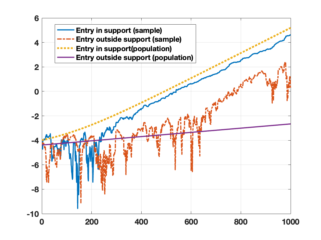
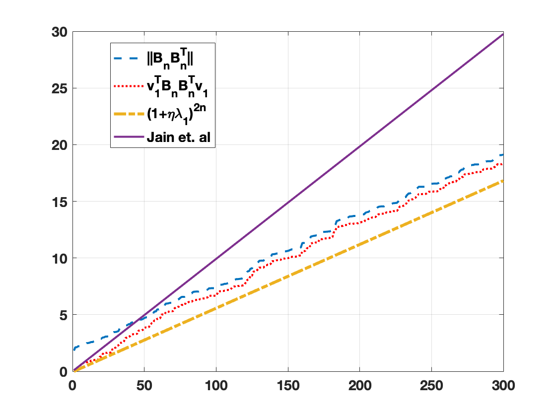
Figure 1: We use $\Sigma=\lambda_{1}v_{1}v_{1}^{T}+\sigma^{2}I$ with $\lambda_{1}=5,\sigma=1$, $d=1000$. (A) Variation of $\log\left(|e_{i}^{\top}B_{n}u_{0}|\right)$ for $i\in S$ and $i\notin S$ with $n$ for a fixed unit vector $u_{0}$. We use $\Sigma=\lambda_{1}v_{1}v_{1}^{T}+\sigma^{2}I$ with $\lambda_{1}=5,\sigma=1$, $d=1000$. $v_{1}\left(i\right)=\frac{1}{\sqrt{s}}$ for $s=10$. $\eta$ is set as Theorem 1 and $n$ grows from $1$ to $1000$. (B) Variation of $\log\left(\left\lVert B_{n}B_{n}^{T}\right\rVert\right)$ and $\log\left(v_{1}^{T}B_{n}B_{n}^{T}v_{1}\right)$ with $n\in[300]$. We also plot $\log$ of the bound of $\left\lVert B_{n}B_{n}^{T}\right\rVert$ as in [20] and $2n\log\left(1+\eta\lambda_{1}\right)$ for comparison.

However, Figure 1(A) shows that while the elements in the support seem close to their expectation, those not in support are, on average, much larger than their expectation. First, note that elementwise analysis of the Oja vector has not been done even in the low dimensional regime where $r_{\text{eff}}/n\rightarrow 0$. In the high-dimensional case, an analog can be drawn with elements of the sample covariance matrix. Here, all elements concentrate around their mean individually, and yet the overall matrix does not concentrate around the population covariance matrix. This leads to thresholding of the sample covariance matrix to obtain consistent estimates of the population under sparsity assumptions [4, 9, 36]. A similar principle is applied by [43] where they truncate the elements of the eigenvector of an empirical covariance matrix. While our method is based on the same principle, the analysis is completely different, because as we will show, the entries do not concentrate even for $i\in S$. But one can show that, for a suitably chosen threshold, the elements in the support are much larger with high probability, whereas those outside are much lower with high probability. Proving this is also difficult because the analysis involves the concentration of the projection of a product of independent high dimensional matrices on some initial random vector.

As it turns out, Lemma 1 establishes exactly that for elements in the support. [Tail bound in support] Fix a $\delta\in\left(0.1,1\right)$. Define the event $\mathcal{G}:=\left\{|v_{1}^{T}y_{0}|\geq\frac{\delta}{\sqrt{e}}\right\}$ and threshold $\tau_{n}:=\frac{\delta}{\sqrt{2e}}\min_{i\in S_{\text{hi}}}|v_{1}\left(i\right)|\left(1+\eta\lambda_{1}\right)^{n}$. Let the learning rate be set as in Theorem 3.3. Then,

$$\forall i\in S,\;\;\;\;\mathbb{P}\left(|r_{i}|\leq\tau_{n}\bigg{|}\mathcal{G}\right)\leq C_{H}\left[\eta\lambda_{1}\log\left(n\right)+\eta\lambda_{1}\left(\frac{\lambda_{1}}{\lambda_{1}-\lambda_{2}}\right)\frac{1}{v_{1}\left(i\right)^{2}}\right]$$

where $C_{H}>0$ is an absolute constant. Our next result provides a bound for $i\notin S$. [Tail bound outside support] Fix a $\delta\in\left(0.1,1\right)$. Let the learning rate be set as in Theorem 3.3 and define the threshold $\tau_{n}:=\frac{\delta}{\sqrt{2e}}\min_{i\in S_{\text{hi}}}|v_{1}\left(i\right)|\left(1+\eta\lambda_{1}\right)^{n}$. Then, for $n=\widetilde{\Omega}\left(\frac{1}{\delta^{2}\min_{i\in S_{\text{hi}}}v_{1}\left(i\right)^{2}}\right)$ we have,

$$\forall i\notin S,\;\;\;\;\mathbb{P}\left(|r_{i}|>\tau_{n}\right)\leq C_{T}\left[\eta^{2}\lambda_{1}^{2}\left(\frac{\lambda_{1}}{\lambda_{1}-\lambda_{2}}\right)^{2}\left(\frac{1}{\delta^{2}\min_{i\in S_{\text{hi}}}v_{1}\left(i\right)^{2}}\right)^{2}\right]$$

where $C_{T}>0$ is an absolute constant. The proofs of Lemmas 1 and  3.2 are based on tail-bounds involving the second and fourth moments of $r_{i}:=e_{i}^{T}B_{n}y_{0}$. In Section 4, we provide an outline of how to bound the moments and discuss the significance of initialization with a random gaussian vector. The details of obtaining the tail bounds are deferred to the Appendix Section A.3. These lemmas control the deviation of the entries of the output of Oja’s algorithm. They further show intuitively that a truncation on the right threshold would lead to most entries in the support being selected, and most entries outside the support being removed with probability at least $3/4$. The results developed in this section along with Lemma 3.3 are then used to analyze the support recovery and error guarantees of Algorithm 1.

4 Proof Technique

In this section, we outline our proof techniques for Theorem 1. We divide the proof into two broad parts. The first part of the proof analyzes the performance of Oja’s algorithm given an estimated support set for truncation, provided in Theorem 3.3. The second part deals with obtaining a good estimated support set, $\widehat{S}$, using Oja’s Algorithm followed by selecting the top-k largest elements, which uses the entrywise deviation bounds provided in Lemmas 1 and 3.2. Recall that we initialize Oja’s algorithm in both cases with a randomly chosen $u_{0}\sim\mathcal{N}\left(0,I\right)$. The analysis of both parts of Algorithm 1 requires bounds on the expectation and second moment of $u_{0}^{T}B_{n}UU^{T}B_{n}u_{0}$, where $U\in\mathbb{R}^{d\times k}$ is a fixed matrix, chosen appropriately. For the proof sketch, we describe our techniques to bound $\mathbb{E}\left[u_{0}^{T}B_{n}UU^{T}B_{n}u_{0}\right]$ in Section 4.1 and discuss the importantance of the initialization choice for Lemmas 1, 3.2 in Section 4.2.

4.1 Solving a linear system of recursions

Note that, using Lemma A.11 in Appendix Section A.1,

$$\mathbb{E}\left[u_{0}^{T}B_{n}^{T}UU^{T}B_{n}u_{0}\right]=\underbrace{\mathbb{E}\left[v_{1}^{T}B_{n}^{T}UU^{T}B_{n}v_{1}\right]}_{:=\alpha_{n}}+\underbrace{\mathbb{E}\left[\operatorname{Tr}\left(V_{\perp}^{T}B_{n}^{T}UU^{T}B_{n}V_{\perp}\right)\right]}_{:=\beta_{n}}$$ (10)

We start by showing how to bound $\alpha_{n}$ and $\beta_{n}$. Before we dive into our techniques, we note that the analysis of Oja’s algorithm ( [20]) in the non-sparse setting provides some tools that we could potentially use here. Using the recursion from Lemma 9 in  [20], we get

$$\left\lVert\mathbb{E}\left[B_{n}UU^{T}B_{n}^{T}\right]\right\rVert\leq\exp(2n\eta\lambda_{1}+n\eta^{2}\mathcal{V})\left\lVert UU^{T}\right\rVert,$$ (11)

where $\mathcal{V}$ is a variance parameter defined as $\left\lVert\mathbb{E}\left[(A_{1}-\Sigma)(A_{1}-\Sigma)^{T}\right]\right\rVert$. Lemma A.3 shows that for $\sigma$-subgaussian $X$ (definition 2.1),

$$\mathcal{V}:=\left\lVert\mathbb{E}\left[(A_{1}-\Sigma)(A_{1}-\Sigma)^{T}\right]\right\rVert=\left\lVert\mathbb{E}\left[A_{1}A_{1}^{T}\right]-\Sigma^{2}\right\rVert\leq 2L^{4}\sigma^{4}\lambda_{1}\operatorname{Tr}(\Sigma)+\lambda_{1}^{2}$$

This provides an upper bound on $\alpha_{n}\leq\left\lVert\mathbb{E}\left[B_{n}UU^{T}B_{n}^{T}\right]\right\rVert$. While this bound is tight when $\operatorname{Tr}(\Sigma)$ is bounded by a constant, in the high dimensional setting (Assumption 2) considered in this work, this bound is too loose. This is evident from Figure 1(B), which plots $\left\lVert\mathbb{E}\left[B_{n}UU^{T}B_{n}^{T}\right]\right\rVert$ for $U=I$, along with the bound achieved using Eq 11, marked as Jain et al. (2016). Note that the plots are in the $\log$-scale so a difference in the slopes translates to a significant multiplicative difference. This warrants a more fine-grained analysis of $\alpha_{n}$.

Let us examine $\alpha_{n}$ more closely to obtain a finer bound. Using the structure of the matrix product, $B_{n}$, from Eq 4, we have:

$$\alpha_{n} =\alpha_{n-1}\left(1+2\eta\lambda_{1}\right)+\eta^{2}\mathbb{E}\left[\left(v_{1}^{T}X_{n}X_{n}^{T}v_{1}\right)\left(X_{n}^{T}B_{n-1}UU^{T}B_{n-1}^{T}X_{n}\right)\right]$$

$$\leq\alpha_{n-1}\left(1+2\eta\lambda_{1}\right)+\eta^{2}\mathbb{E}\left[\sqrt{\mathbb{E}\left[\left(v_{1}^{T}X_{n}X_{n}^{T}v_{1}\right)^{2}\bigg{|}\mathcal{F}_{n-1}\right]\mathbb{E}\left[\left(X_{n}^{T}B_{n-1}UU^{T}B_{n-1}^{T}X_{n}\right)^{2}\bigg{|}\mathcal{F}_{n-1}\right]}\right]$$

Now, as a consequence of subgaussianity (see Lemma A.2), for $K:=(2L^{2}\sigma^{2})^{2}$ the above can be bounded further as:

$$\mathbb{E}\left[(v_{1}^{T}X_{n}X_{n}^{T}v_{1})^{2}\right]\leq K\lambda_{1}^{2},\;\;\mathbb{E}\left[\left(X_{n}^{T}B_{n-1}UU^{T}B_{n-1}^{T}X_{n}\right)^{2}\bigg{|}\mathcal{F}_{n-1}\right]\leq K\operatorname{Tr}(U^{T}B_{n-1}^{T}\Sigma B_{n-1}U)^{2}$$

Therefore, using the above bound along with the eigendecomposition $\Sigma:=\lambda_{1}v_{1}v_{1}^{T}+V_{\perp}\Lambda_{2}V_{\perp}^{T}$,

$$\alpha_{n} \leq\alpha_{n-1}\left(1+2\eta\lambda_{1}\right)+4\eta^{2}L^{4}\sigma^{4}\lambda_{1}\mathbb{E}\left[\operatorname{Tr}(U^{T}B_{n-1}^{T}\Sigma B_{n-1}U)\right]$$

$$\leq\left(1+2\eta\lambda_{1}+4L^{2}\eta^{2}\sigma^{4}\lambda_{1}^{2}\right)\alpha_{n-1}+4L^{2}\eta^{2}\sigma^{4}\lambda_{1}\lambda_{2}\beta_{n-1}$$ (12)

Similarly, $\beta_{n}$ can also be upper bounded as follows:

$$\beta_{n}\leq\left(1+2\eta\lambda_{2}+4\eta^{2}L^{4}\sigma^{4}\lambda_{2}\operatorname{Tr}\left(\Sigma\right)\right)\beta_{n-1}+4\eta^{2}L^{4}\sigma^{4}\lambda_{1}\operatorname{Tr}\left(\Sigma\right)\alpha_{n-1}$$ (13)

Note that upper bounding and eliminating $\alpha_{n-1}$ or $\beta_{n-1}$ from Eq 13,  12 respectively, would simplify the recursion but lead to a weaker bound as in Eq 11. Therefore, we solve Eq 12 and 13 as a system of linear recursions in $\alpha_{n}$ and $\beta_{n}$.

$$\begin{pmatrix}\alpha_{n}\\ \beta_{n}\end{pmatrix}=\underbrace{\begin{pmatrix}1+2\eta\lambda_{1}+O\left(\eta^{2}\lambda_{1}^{2}\right)&O\left(\lambda_{1}\lambda_{2}\right)\\ O\left(\operatorname{Tr}(\Sigma)\right)&1+2\eta\lambda_{2}+O\left(\eta^{2}\operatorname{Tr}(\Sigma)\right)\end{pmatrix}}_{:=P}\begin{pmatrix}\alpha_{n-1}\\ \beta_{n-1}\end{pmatrix}$$ (14)

Here, the $O(.)$ notation hides constant factors of only model-dependent parameters, $\sigma$ and $L$. Now, everything essentially reduces to estimating elements of $P^{n}$ where $P$ is the $2\times 2$ matrix defined above. [51] provides a compact expression for these elements in terms of $\lambda_{1}(P)$ and $\lambda_{2}(P)$. Through our assumptions, we establish that $P_{11}>P_{22}$. Note that a naive upper bound using Weyl’s inequality (see e.g. [12]) on $\lambda_{1}(P)$ will be $1+2\eta\lambda_{1}+c_{3}\operatorname{Tr}(\Sigma)$, which is much like the one in Eq 11. Since recursions of the form Eq 14 often arise in our analysis, we provide a general solution in Lemma 4.1 (see Lemma A.6 in Appendix Section A.1 for detailed result).

Lemma 4.1 (Matrix Recursion).

Consider the following system of recursions for constant $c_{1}>0$,

$$\alpha_{n} =\left(1+c_{1}\eta\lambda_{1}+O\left(\eta^{2}\lambda_{1}^{2}\right)\right)\alpha_{n-1}+O\left(\eta^{2}\lambda_{1}\lambda_{2}\right)\beta_{n-1},$$

$$\beta_{n} =\left(1+c_{1}\eta\lambda_{2}+O\left(\eta^{2}\lambda_{2}\operatorname{Tr}\left(\Sigma\right)\right)\right)\beta_{n-1}+O\left(\eta^{2}\lambda_{1}\operatorname{Tr}\left(\Sigma\right)\right)\alpha_{n-1}$$

Under Assumption 2, there exists a learning rate $\eta$, such that,

$$\alpha_{n} =\lambda_{1}\left(P\right)^{n}\left(\alpha_{0}(1+O(\eta\lambda_{1}))+O\left(\frac{\eta\lambda_{1}^{2}}{\lambda_{1}-\lambda_{2}}\right)\beta_{0}\right),$$

$$\beta_{n} =\lambda_{1}(P)^{n}\frac{\eta\lambda_{1}^{2}}{\lambda_{1}-\lambda_{2}}\left(\alpha_{0}\frac{\operatorname{Tr}(\Sigma)}{\lambda_{1}}+O(\beta_{0})\right)+\lambda_{2}\left(P\right)^{n}$$

where $\left|\lambda_{1}\left(P\right)-P_{11}\right|,\left|\lambda_{2}\left(P\right)-P_{22}\right|=O\left(\eta^{2}\lambda_{1}^{2}\right)$.

Here the $O(.)$ notation hides constant depending only on $\sigma$ and $L$. The above equations simply say that the large $\operatorname{Tr}(\Sigma)$ term is does not affect the largest eigenvalue of $P$. An important consequence of this is that we now have the following bounds on $\alpha_{n}$ and $\beta_{n}$ for $U=I$:

$$\mathbb{E}\left[v_{1}^{T}B_{n}B_{n}v_{1}\right] \leq(1+2\eta\lambda_{1}+c_{1}\eta^{2}\lambda_{1}^{2})^{n}\left(1+O(\eta\lambda_{1})\right)$$

$$\approx\left(1+O\left(\eta\lambda_{1}\right)\right)\exp\left(2\eta n\lambda_{1}+c^{\prime}\eta^{2}n\lambda_{1}^{2}\right)$$ (15)

which is much tighter than Eq 11 in our high-dimensional regime. Furthermore, observing Figure 1(B), we see that Eq 15 presents a much tighter upper bound, matching $\left(1+\eta\lambda_{1}\right)^{2n}$ up to constant factors. Lemma 4.1 provides insights into the proofs of Theorem 3.3 and Lemmas 1, 3.2. The proof of Theorem 3.3, sets $UU^{T}$ as either the $W_{\widehat{S}}$ or $G_{\widehat{S}}$ matrices appropriately. Similarly, for Lemmas 1,3.2 we select $U=e_{i}$ for both $i\in S$ and $i\notin S$.

Recall that the bounds obtained in this section deal with $\alpha_{n}=\mathbb{E}\left[v_{1}^{T}B_{n}^{T}UU^{T}B_{n}v_{1}\right]$
and $\beta_{n}=\mathbb{E}\left[\operatorname{Tr}\left(V_{\perp}^{T}B_{n}^{T}UU^{T}B_{n}V_{\perp}\right)\right]$. A similar system of recursions can be obtained to get tight bounds on $\mathbb{E}\left[\left(v_{1}^{T}B_{n}^{T}UU^{T}B_{n}v_{1}\right)^{2}\right]$ and $\mathbb{E}\left[\operatorname{Tr}\left(V_{\perp}^{T}B_{n}^{T}UU^{T}B_{n}V_{\perp}\right)^{2}\right]$, details of which we defer to the Appendix Lemmas A.9 and A.10.

4.2 Importance of random initialization

Now that we have established moment bounds for $u_{0}^{T}B_{n}UU^{T}B_{n}u_{0}$ for $u_{0}\sim\mathcal{N}\left(0,I\right)$, we briefly discuss the significance of the initialization from the perspective of Lemmas 1 and 3.2. Note that choosing only a fixed $u_{0}\in\mathbb{R}^{d}$ is not sufficient, since in the worst case, $v_{1}\perp u_{0}$, which would lead to $\mu=v_{1}^{T}u_{0}=0$. Standard anti-concentration results for the chi-squared random variable (see Lemma A.1) imply that for $\delta\in\left(0,1\right)$, with probability at least $1-\delta$,   $|v_{1}^{T}u_{0}|\geq\frac{\delta}{\sqrt{e}}$. Recall the choice of the threshold $\tau_{n}:=\frac{\delta}{\sqrt{2e}}\min_{i\in S_{\text{hi}}}|v_{1}\left(i\right)|\left(1+\eta\lambda_{1}\right)^{n}$. Then, for entries in the support, projecting $u_{0}$ in the direction of $v_{1}$ and its orthogonal subspace, we obtain with probability at least $1-\delta$, that entries in the support are larger than $\tau_{n}$. Entries outside the support are shown to be smaller than $\tau_{n}$ with probability at least $1-\delta$ using a second moment bound on $r_{i}^{2}=u_{0}^{T}B_{n}^{T}e_{i}e_{i}^{T}B_{n}u_{0}$ for $i\notin S$. The details of this argument can be found in Appendix Section A.3.

5 Conclusion

Oja’s algorithm for streaming PCA has received a lot of attention in the recent theoretical literature. However, the optimal guarantees are all in the setting where the datapoints are bounded a.s. or the trace of the covariance matrix is growing slowly with $n$. In this paper, we tackle the high-dimensional setting where the effective rank $r_{\text{eff}}$ can be as large as some constant fraction of $n$ but the underlying eigenvector is $s$-sparse. In this setting, the error rate of Oja’s algorithm without any modifications is $O(r_{\text{eff}}/n)$. However, our thresholded estimator achieves a near-optimal error rate of $O(s\log d/n)$. Empirically, we see that the elements of the unnormalized Oja vector do not concentrate in this regime. However, with an analysis that carefully uncouples the projection of a product of independent random matrices on $v_{1}$ and the orthogonal subspace, we can establish that the entries of the Oja vector in the support of $v_{1}$ are large, whereas those outside are much smaller.

The Appendix is organized as follows:

1. Section A.1 provides useful helper lemmas

2. Section A.2 proves Convergence of Oja’s algorithm with truncation (Theorem 3.3)

3. Section A.3 provides deviation bounds for entries of the Oja vector (Lemmas 1 and 3.2)

4. Section A.4 provides proofs of our main result for Sparse PCA (Theorem 1) and provides another alternative way of truncation using a value-based thresholding (Theorem 2)

Appendix A.1 Useful Lemmas

Lemma A.1.

(Fact 2.9 [11]) For any symmetric $d\times d$ matrix A, we have $\operatorname{Var}_{z\sim\mathcal{N}\left(0,I\right)}\left[z^{T}Az\right]=2\|A\|_{F}^{2}$. If A is a PSD matrix, then for any $\beta>0$, it holds that

$$\mathbb{P}_{z\sim\mathcal{N}\left(0,I\right)}\left[z^{T}Az\geq\beta\operatorname{Tr}\left(A\right)\right]\geq 1-\sqrt{e\beta}$$

Proof.

We give a short proof here. Since A is a symmetric matrix, let $A=P\Lambda P^{T}$ where $P$ is an orthonormal matrix and $\Lambda$ is a diagonal matrix. Then, denoting $y:=P^{T}z$ we note that $y\sim\mathcal{N}\left(0,I\right)$. Therefore,

$$z^{T}Az =z^{T}P\Lambda P^{T}z=y^{T}\Lambda y=\sum_{i=1}^{d}\lambda_{i}y_{i}^{2}$$

Therefore,

$$\mathbb{E}_{z\sim\mathcal{N}\left(0,I\right)}\left[z^{T}Az\right]=\mathbb{E}_{y\sim\mathcal{N}\left(0,I\right)}\left[\sum_{i=1}^{d}\lambda_{i}y_{i}^{2}\right]=\sum_{i=1}^{d}\lambda_{i}=\operatorname{Tr}\left(A\right)$$

and

$$\mathbb{E}_{z\sim\mathcal{N}\left(0,I\right)}\left[\left(z^{T}Az\right)^{2}\right]=\mathbb{E}_{y\sim\mathcal{N}\left(0,I\right)}\left[\left(\sum_{i=1}^{d}\lambda_{i}y_{i}^{2}\right)^{2}\right] =\mathbb{E}_{y\sim\mathcal{N}\left(0,I\right)}\left[\sum_{i=1}^{d}\lambda_{i}^{2}y_{i}^{4}+\sum_{i,j,i\neq j}^{d}\lambda_{i}\lambda_{j}y_{i}^{2}y_{j}^{2}\right]$$

$$=3\sum_{i=1}^{d}\lambda_{i}^{2}+\sum_{i,j,i\neq j}^{d}\lambda_{i}\lambda_{j}=2\operatorname{Tr}\left(A^{2}\right)+\operatorname{Tr}\left(A\right)^{2}$$

To get the tail lower bound, note that it trivially follows if $\beta>1$. Therefore we proceed with $\beta\in\left(0,1\right)$. We have

$$\mathbb{P}_{z\sim\mathcal{N}\left(0,I\right)}\left[z^{T}Az\leq\beta\operatorname{Tr}\left(A\right)\right] =\mathbb{P}_{y\sim\mathcal{N}\left(0,I\right)}\left[\sum_{i=1}^{d}\lambda_{i}y_{i}^{2}\leq\beta\sum_{i=1}^{d}\lambda_{i}\right]$$

$$\leq\mathbb{E}\left[\exp\left(t\left(\beta\sum_{i=1}^{d}\lambda_{i}-\sum_{i=1}^{d}\lambda_{i}y_{i}^{2}\right)\right)\right],t>0$$

$$=\exp\left(t\beta\sum_{i=1}^{d}\lambda_{i}\right)\mathbb{E}\left[\exp\left(-t\sum_{i=1}^{d}\lambda_{i}y_{i}^{2}\right)\right]$$

$$=\exp\left(t\beta\sum_{i=1}^{d}\lambda_{i}\right)\prod_{i=1}^{d}\left(1+2\lambda_{i}t\right)^{-\frac{1}{2}}$$

Let $t=\frac{1}{2\sum_{i=1}^{d}\lambda_{i}}\left(\frac{1}{\beta}-1\right)$. Then,

$$\mathbb{P}_{z\sim\mathcal{N}\left(0,I\right)}\left[z^{T}Az\leq\beta\operatorname{Tr}\left(A\right)\right] \leq\exp\left(\frac{1-\beta}{2}\right)\prod_{i=1}^{d}\left(1+\frac{\lambda_{i}}{\sum_{i=1}^{d}\lambda_{i}}\left(\frac{1}{\beta}-1\right)\right)^{-\frac{1}{2}}$$

$$\leq\exp\left(\frac{1-\beta}{2}\right)\left(1+\left(\frac{1}{\beta}-1\right)\right)^{-\frac{1}{2}}$$

$$=\exp\left(\frac{1-\beta}{2}\right)\sqrt{\beta}$$

$$\leq\sqrt{e\beta}$$

Hence proved. ∎

Lemma A.2.

Let $X\in\mathbb{R}^{d}$ be a $\sigma$-subgaussian random vector with covariance matrix $\Sigma$. Then, for any matrix $M\in\mathbb{R}^{d\times m}$ and any positive integer $p\geq 2$,

$$\mathbb{E}\left[\left(X^{T}MM^{T}X\right)^{p}\right]\leq\left(L^{2}\sigma^{2}p\right)^{p}\operatorname{Tr}\left(M^{T}\Sigma M\right)^{p}$$

Proof.

Let the eigendecomposition of $MM^{T}$ be $P\Lambda P^{T}$. Define $Y:=P^{T}X$. Then,

$$\mathbb{E}\left[\left(X^{T}MM^{T}X\right)^{p}\right] =\mathbb{E}\left[\left(\sum_{i=1}^{d}\lambda_{i}y_{i}^{2}\right)^{p}\right]$$

$$=\sum_{k_{1}+k_{2}+\cdots k_{d}=p;\;k_{1},k_{2},\cdots k_{d}\geq 0}{n\choose k_{1},k_{2},\cdots k_{d}}\mathbb{E}\left[\prod_{i=1}^{d}\lambda_{i}^{k_{i}}y_{i}^{2k_{i}}\right]$$ (A.16)

Therefore,

$$\mathbb{E}\left[\prod_{i=1}^{d}\lambda_{i}^{k_{i}}y_{i}^{2k_{i}}\right] =\left(\prod_{i=1}^{d}\lambda_{i}^{k_{i}}\right)\mathbb{E}\left[\prod_{i=1}^{d}y_{i}^{2k_{i}}\right]$$

$$\leq\left(\prod_{i=1}^{d}\lambda_{i}^{k_{i}}\right)\prod_{i=1}^{d}\left(\mathbb{E}\left[\left(y_{i}^{2k_{i}}\right)^{\frac{p}{k_{i}}}\right]\right)^{\frac{k_{i}}{p}},\text{ using Holder's inequality since }\sum_{i=1}^{d}k_{i}=p,$$

$$=\left(\prod_{i=1}^{d}\lambda_{i}^{k_{i}}\right)\prod_{i=1}^{d}\left(\mathbb{E}\left[y_{i}^{2p}\right]\right)^{\frac{k_{i}}{p}}$$ (A.17)

Using the definition of sub-gaussianity (Definition 2.1) we have,

$$\mathbb{E}\left[y_{i}^{2p}\right] =\mathbb{E}\left[\left(e_{i}^{T}P^{T}X\right)^{2p}\right]$$

$$=\mathbb{E}\left[\left(\left(Pe_{i}\right)^{T}X\right)^{2p}\right]$$

$$\leq L^{2p}\sigma^{2p}\left(\sqrt{p}\right)^{2p}\left(\left\lVert Pe_{i}\right\rVert_{\Sigma}\right)^{2p}$$

$$=L^{2p}\sigma^{2p}p^{p}\left(e_{i}^{T}P^{T}\Sigma Pe_{i}\right)^{p}$$

Susbstituting in Eq A.17 we have,

$$\mathbb{E}\left[\prod_{i=1}^{d}\lambda_{i}^{k_{i}}y_{i}^{2k_{i}}\right] \leq\left(\prod_{i=1}^{d}\lambda_{i}^{k_{i}}\right)\left(\prod_{i=1}^{d}L^{2k_{i}}\sigma^{2k_{i}}p^{k_{i}}\left(e_{i}^{T}P^{T}\Sigma Pe_{i}\right)^{k_{i}}\right)$$

$$=\left(L^{2}\sigma^{2}p\right)^{p}\prod_{i=1}^{d}\left(\lambda_{i}e_{i}^{T}P^{T}\Sigma Pe_{i}\right)^{k_{i}}$$

Substituting in Eq A.16 we have,

$$\mathbb{E}\left[\left(X^{T}MM^{T}X\right)^{p}\right] \leq\left(L^{2}\sigma^{2}p\right)^{p}\sum_{k_{1}+k_{2}+\cdots k_{d}=p;\;k_{1},k_{2},\cdots k_{d}\geq 0}{n\choose k_{1},k_{2},\cdots k_{d}}\prod_{i=1}^{d}\left(\lambda_{i}e_{i}^{T}P^{T}\Sigma Pe_{i}\right)^{k_{i}}$$

$$=\left(L^{2}\sigma^{2}p\right)^{p}\left(\sum_{i=1}^{d}\lambda_{i}e_{i}^{T}P^{T}\Sigma Pe_{i}\right)^{p}$$

$$=\left(L^{2}\sigma^{2}p\right)^{p}\left(\operatorname{Tr}\left(\left(\sum_{i=1}^{d}\lambda_{i}Pe_{i}e_{i}^{T}P^{T}\right)\Sigma\right)\right)^{p}=\left(L^{2}\sigma^{2}p\right)^{p}\operatorname{Tr}\left(M^{T}\Sigma M\right)^{p}$$

Hence proved. ∎

Lemma A.3.

Let $X\in\mathbb{R}^{d}$ be a $\sigma$-subgaussian random vector with covariance matrix $\Sigma$. Then,

$$\left\lVert\mathbb{E}\left[\left(XX^{T}\right)^{2}\right]\right\rVert\leq 4L^{4}\sigma^{4}\lambda_{1}\operatorname{Tr}\left(\Sigma\right)$$

Proof.

For any fixed unit vector $u\in\mathbb{R}^{d}$, we have

$$u^{T}\mathbb{E}\left[\left(XX^{T}\right)^{2}\right]u =\mathbb{E}\left[\left(X^{T}X\right)\left(X^{T}u\right)^{2}\right]$$

$$\leq\sqrt{\mathbb{E}\left[\left(X^{T}X\right)^{2}\right]\mathbb{E}\left[\left(X^{T}u\right)^{4}\right]}$$

$$=\sqrt{\mathbb{E}\left[\left(X^{T}X\right)^{2}\right]\mathbb{E}\left[\left(X^{T}uu^{T}X\right)^{2}\right]}$$

$$\leq\left(2L^{2}\sigma^{2}\right)^{2}\operatorname{Tr}\left(\Sigma\right)\operatorname{Tr}\left(u^{T}\Sigma u\right)$$

$$\leq\left(2L^{2}\sigma^{2}\right)^{2}\lambda_{1}\operatorname{Tr}\left(\Sigma\right)$$

where we used Lemma A.2 with $p=2$ and $M=I$. ∎

Lemma A.4.

(Boosting using Geometric Aggregation) Let $u_{*}\in\mathbb{R}^{d}$ be a fixed unit vector and $u_{1},u_{2},\cdots u_{r}\in\mathbb{R}^{d}$ be $r$ independent random unit vectors each satisfying $\mathbb{P}\left(\sin^{2}\left(u_{i},u_{*}\right)\geq\epsilon\right)\leq p$ for a constant $p\in\left(0,\frac{1}{2}\right)$. There there is an estimator $\tilde{u}$ which selects one of $\left\{u_{i}\right\}_{i\in[r]}$, runs in $O\left(r^{2}d\right)$ time and satisfies,

$$\mathbb{P}\left(\sin^{2}\left(\tilde{u},u_{*}\right)\geq 9\epsilon\right)\leq\exp\left(-\frac{\left(1-p\right)r}{20}\right)$$

Proof.

Consider the indicator random variables $\chi_{i}:=\mathbbm{1}\left(\sin^{2}\left(u_{i},u_{*}\right)\leq\epsilon\right)$. Then, $\forall i\in[r],\;\mathbb{P}\left(\chi_{i}=1\right)\geq 1-p$. Define the set $\mathcal{S}:=\left\{i:\chi_{i}=1\right\}$. We note that using standard Chernoff bounds for sums of independent Bernoulli random variables, for $\delta\in\left(0,1\right)$,

$$\mathbb{P}\left(|\mathcal{S}|\leq\left(1-\delta\right)\mathbb{E}\left[|\mathcal{S}|\right]\right)\leq\exp\left(-\frac{\delta^{2}\mathbb{E}\left[|\mathcal{S}|\right]}{2}\right)$$

We have, $\mathbb{E}\left[|\mathcal{S}|\right]\geq r\left(1-p\right)$ using linearity of expectation. Therefore,

$$\;\;\;\;\;\;\;\;\;\mathbb{P}\left(|\mathcal{S}|\leq\left(1-\delta\right)\left(1-p\right)r\right)\leq\exp\left(-\frac{\delta^{2}\left(1-p\right)r}{2}\right)$$

$$\implies\mathbb{P}\left(|\mathcal{S}|\leq 0.6\left(1-p\right)r\right)\leq\exp\left(-\frac{\left(1-p\right)r}{20}\right),\text{ for }\delta:=\sqrt{\frac{1}{10}}$$ (A.18)

We define $\tilde{u}$ as:

$$\tilde{u}:=u_{i},\text{ such that }\frac{\left|\left\{j\in[r]:\sin^{2}\left(u_{i},u_{j}\right)\leq 4\epsilon\right\}\right|}{r}\geq 0.6\left(1-p\right)$$ (A.19)

Note that the definition of $\tilde{u}$ does not require knowledge of $u_{*}$ and it can be computed by calculating $\sin^{2}$ error between all distinct ${r\choose 2}$ pairs $\left(u_{i},u_{j}\right)_{i,j\in[r],i\neq j}$.

Let $\mathcal{E}$ be the event $\{|\mathcal{S}|>0.6\left(1-p\right)r\}$ and denote $f:=0.6\left(1-p\right)$ for convenience of notation. Let us now operate conditioned on $\mathcal{E}$. Note that conditioned on $\mathcal{E}$, such a $\tilde{u}$ always exists since any point in $\mathcal{S}$ is a valid selection of $\tilde{u}$. This is true since

$$\left\lVert u_{i}u_{i}^{T}-u_{j}u_{j}^{T}\right\rVert_{F}\leq\left\lVert u_{i}u_{i}^{T}-u_{*}u_{*}^{T}\right\rVert_{F}+\left\lVert u_{j}u_{j}^{T}-u_{*}u_{*}^{T}\right\rVert_{F}\leq 2\sqrt{2\epsilon}$$

Here we used Definition 3 and the property of the event $\mathcal{E}$. We further have, conditioned on $\mathcal{E}$ using triangle inequality for some $i\in\mathcal{S}$,

$$\left\lVert\tilde{u}\tilde{u}^{T}-u_{*}u_{*}^{T}\right\rVert_{F}\leq\left\lVert\tilde{u}\tilde{u}^{T}-u_{i}u_{i}^{T}\right\rVert_{F}+\left\lVert u_{i}u_{i}^{T}-u_{*}u_{*}^{T}\right\rVert_{F}\leq 3\sqrt{2\epsilon}$$ (A.20)

Therefore, we have

$$\mathbb{P}\left(\sin^{2}\left(\tilde{u},u_{*}\right)\geq 9\epsilon\right) =\mathbb{P}\left(\mathcal{E}\right)\mathbb{P}\left(\sin^{2}\left(\tilde{u},u_{*}\right)\geq 9\epsilon|\mathcal{E}\right)+\mathbb{P}\left(\mathcal{E}^{c}\right)\mathbb{P}\left(\sin^{2}\left(\tilde{u},u_{*}\right)\geq 9\epsilon|\mathcal{E}^{c}\right)$$

$$=0+\mathbb{P}\left(\mathcal{E}^{c}\right)\mathbb{P}\left(\sin^{2}\left(\tilde{u},u_{*}\right)\geq 9\epsilon|\mathcal{E}^{c}\right)\text{ using Eq\leavevmode\nobreak\ \ref{eq:u_tilde_good_event_bound}}$$

$$\leq\mathbb{P}\left(\mathcal{E}^{c}\right)$$

$$\leq\exp\left(-\frac{\left(1-p\right)r}{20}\right)\text{ using Eq\leavevmode\nobreak\ \ref{eq:chernoff_bernoulli}}$$

which completes our proof. ∎

Lemma A.5 (Learning rate schedule).

Let the learning rate be set as $\eta:=\frac{\kappa\log\left(n\right)}{n\left(\lambda_{1}-\lambda_{2}\right)}$. Then, under Assumptions 2 and 3, for

$$3\leq\kappa\leq\frac{1}{2C\alpha},\;\;n\geq\max\left\{sC\left(\kappa\frac{\lambda_{1}\log\left(n\right)}{\lambda_{1}-\lambda_{2}}\right)^{2},\;\frac{s}{9}\left(\frac{\lambda_{1}-\lambda_{2}}{\lambda_{1}\log\left(n\right)}\right)^{2},\;100s\right\}$$

the following hold:

1. $\eta\leq\frac{1}{C\log\left(n\right)}\frac{\left(\lambda_{1}-\lambda_{2}\right)}{\lambda_{2}\operatorname{Tr}\left(\Sigma\right)}$

2. $C\eta\leq\frac{1}{4}\min\left\{\frac{1}{s\lambda_{1}},\frac{\log\left(n\right)}{\operatorname{Tr}\left(\Sigma\right)},\frac{\log\left(n\right)}{\sqrt{\lambda_{1}\operatorname{Tr}\left(\Sigma\right)}}\right\}$

3. $C\eta^{2}n\lambda_{1}^{2}\leq\frac{1}{g_{2}}\eta\lambda_{1}\log\left(n\right)\leq\frac{1}{4}$

4. $\exp\left(-cn\eta\left(\lambda_{1}-\lambda_{2}\right)\right)\leq\eta\lambda_{1}\;$ for $c\geq\frac{1}{2}$

where

$$C:=100\left(L^{4}\sigma^{4}+L^{2}\sigma^{2}\right)+16,\;W:=C\log^{2}\left(d\right),\text{ and }\frac{\lambda_{1}-\lambda_{2}}{\lambda_{2}}\geq W$$

We state another useful restatement of Claim (1) used in subsequent analysis,

$$\exists\theta\in\left(0.5,1\right),\;\;\left(1-\theta\right)\left(\lambda_{1}-\lambda_{2}\right)+50L^{4}\sigma^{4}\eta\lambda_{1}^{2}=50L^{4}\sigma^{4}\log\left(n\right)\eta\lambda_{2}\operatorname{Tr}\left(\Sigma\right)$$

Proof.

First, we note that

$$\frac{\lambda_{1}}{\lambda_{1}-\lambda_{2}}=\frac{1}{1-\frac{\lambda_{2}}{\lambda_{1}}}\leq\frac{1}{1-\frac{1}{W+1}}\leq 1+\frac{1}{W}\leq 2$$ (A.21)

where the last inequality holds for sufficiently larger $d$. Now, for the first claim, we have

$$\frac{\eta\lambda_{2}\operatorname{Tr}\left(\Sigma\right)}{\left(\lambda_{1}-\lambda_{2}\right)} =\kappa\frac{\log\left(d\right)\lambda_{2}\operatorname{Tr}\left(\Sigma\right)}{n\left(\lambda_{1}-\lambda_{2}\right)^{2}}=\kappa\frac{\log\left(d\right)\lambda_{2}\lambda_{1}}{\left(\lambda_{1}-\lambda_{2}\right)^{2}}\frac{\operatorname{Tr}\left(\Sigma\right)}{n\lambda_{1}}\leq\frac{2\kappa}{W}\log\left(d\right)\alpha$$

$$\;\;\;\;=\frac{2\kappa}{C\log^{2}\left(d\right)}\log\left(d\right)\alpha=\frac{2\kappa\alpha}{C\log\left(d\right)}\stackrel{{\scriptstyle(i)}}{{\leq}}\frac{1}{C\log\left(d\right)}$$

where $(i)$ follows by the definition of $\kappa$. For the second claim, note that

$$C\eta\lambda_{1} =\frac{\kappa\log\left(n\right)C\lambda_{1}}{n\left(\lambda_{1}-\lambda_{2}\right)}\leq\frac{2\kappa\log\left(n\right)C}{n}\leq 2C\frac{\log\left(n\right)}{n}\stackrel{{\scriptstyle(ii)}}{{\leq}}\frac{1}{4s}$$

where $(ii)$ holds since $s=o\left(\frac{d}{\log\left(d\right)}\right)=o\left(\frac{n}{\log\left(n\right)}\right)$ by Assumption 3. Furthermore, using Eq A.21

$$C\eta\operatorname{Tr}\left(\Sigma\right) =C\frac{\kappa\log\left(n\right)\operatorname{Tr}\left(\Sigma\right)}{n\left(\lambda_{1}-\lambda_{2}\right)}=C\alpha\frac{\kappa\lambda_{1}\log\left(n\right)}{\left(\lambda_{1}-\lambda_{2}\right)}\stackrel{{\scriptstyle(iii)}}{{\leq}}\log\left(n\right)$$

where $(iii)$ follows using the definition of $\kappa$. $\eta C\leq\min\left\{\frac{1}{4\lambda_{1}},\frac{1}{4}\frac{\log\left(n\right)}{\operatorname{Tr}\left(\Sigma\right)}\right\}$ imply $4\eta\left(100L^{2}\sigma^{2}+4\right)\leq\frac{\sqrt{\log\left(n\right)}}{\sqrt{\lambda_{1}\operatorname{Tr}\left(\Sigma\right)}}\leq\frac{\log\left(n\right)}{\sqrt{\lambda_{1}\operatorname{Tr}\left(\Sigma\right)}}$ by the AM-GM inequality. For the third claim, we have

$$C\eta^{2}n\lambda_{1}^{2} =C\eta\lambda_{1}\frac{\kappa\log\left(n\right)\lambda_{1}}{\lambda_{1}-\lambda_{2}}\leq 2C\kappa\eta\lambda_{1}\log\left(n\right)=C\frac{\kappa^{2}\log^{2}\left(n\right)\lambda_{1}}{n\left(\lambda_{1}-\lambda_{2}\right)}\stackrel{{\scriptstyle(iv)}}{{\leq}}\frac{1}{4}$$

where $(iv)$ holds for sufficiently large $n$. Next, we have the last claim,

$$\exp\left(-cn\eta\left(\lambda_{1}-\lambda_{2}\right)\right) =\exp\left(-c\kappa\log\left(n\right)\right)=\frac{1}{n^{c\kappa}}$$

Therefore, it suffices to ensure

$$\frac{1}{n^{c\kappa}}\leq\frac{1}{n^{\frac{\kappa}{2}}}\leq\frac{\kappa\lambda_{1}\log\left(n\right)}{n\left(\lambda_{1}-\lambda_{2}\right)}$$

Note that $\frac{\lambda_{1}}{\left(\lambda_{1}-\lambda_{2}\right)}\geq 1$ since $\lambda_{1}>\lambda_{2}$. Therefore, we require

$$\frac{1}{n^{\frac{\kappa}{2}}}\leq\frac{\kappa\log\left(n\right)}{n}$$

which holds for $\kappa\geq 3$ and sufficiently large $n$. Note that for $\kappa$, the upper bound is larger than the lower bound as long as $\alpha\leq\frac{1}{6C}$, which is true by Assumption 2. ∎

Lemma A.6.

For constants $c_{1},c_{2},c_{3},c_{4},c_{5}>0$, consider the following system of recursions -

$$\alpha_{n} \leq\left(1+c_{1}\eta\lambda_{1}+c_{2}\eta^{2}\lambda_{1}^{2}\right)\alpha_{n-1}+c_{3}\eta^{2}\lambda_{1}\lambda_{2}\beta_{n-1},$$

$$\beta_{n} \leq\left(1+c_{1}\eta\lambda_{2}+c_{4}\eta^{2}\lambda_{2}\operatorname{Tr}\left(\Sigma\right)\right)\beta_{n-1}+c_{5}\eta^{2}\lambda_{1}\operatorname{Tr}\left(\Sigma\right)\alpha_{n-1}$$

Let $\exists\theta\in\left(0.5,1\right)$, which satisfies $c_{1}\left(1-\theta\right)\left(\lambda_{1}-\lambda_{2}\right)+c_{2}\eta\lambda_{1}^{2}=c_{4}\eta\lambda_{2}\operatorname{Tr}\left(\Sigma\right)$ and

$$\frac{4c_{3}c_{5}}{c_{1}^{2}}\eta^{2}\lambda_{2}\operatorname{Tr}\left(\Sigma\right)\left(\frac{\lambda_{1}}{\theta\left(\lambda_{1}-\lambda_{2}\right)}\right)^{2}\leq 1,\;\;4\eta\lambda_{1}\left(\frac{c_{2}\lambda_{1}}{c_{1}\left(\lambda_{1}-\lambda_{2}\right)}\right)\leq 1-\theta$$

Then we have,

$$\alpha_{n} \leq\lambda_{1}\left(P\right)^{n}\left[\alpha_{0}+\eta\lambda_{1}\left(\frac{2c_{3}\lambda_{1}}{c_{1}\theta\left(\lambda_{1}-\lambda_{2}\right)}\right)\left(\beta_{0}+\alpha_{0}\frac{c_{5}}{c_{4}}\left(\frac{1-\theta}{\theta}\right)\right)\right],$$

$$\beta_{n} \leq\beta_{0}\lambda_{2}\left(P\right)^{n}+\left[\eta\lambda_{1}\left(\frac{2c_{5}\lambda_{1}}{c_{1}\theta\left(\lambda_{1}-\lambda_{2}\right)}\right)\left(\alpha_{0}\frac{\operatorname{Tr}\left(\Sigma\right)}{\lambda_{1}}+\beta_{0}\frac{c_{3}}{c_{4}}\left(\frac{1-\theta}{\theta}\right)\right)\right]\lambda_{1}\left(P\right)^{n}$$

where

$$\left|\lambda_{1}\left(P\right)-1-c_{1}\eta\lambda_{1}-c_{2}\eta^{2}\lambda_{1}^{2}\right|\leq\frac{c_{3}c_{5}}{c_{4}}\eta^{2}\lambda_{1}^{2}\left(\frac{1-\theta}{\theta}\right)$$

$$\left|\lambda_{2}\left(P\right)-1-c_{1}\eta\lambda_{2}-c_{4}\eta^{2}\lambda_{2}\operatorname{Tr}\left(\Sigma\right)\right|\leq\frac{c_{3}c_{5}}{c_{4}}\eta^{2}\lambda_{1}^{2}\left(\frac{1-\theta}{\theta}\right)$$

Proof.

Writing the recursions in a matrix form, we have

$$\begin{pmatrix}\alpha_{n}\\ \beta_{n}\end{pmatrix}=\begin{pmatrix}1+c_{1}\eta\lambda_{1}+c_{2}\eta^{2}\lambda_{1}^{2}&c_{3}\eta^{2}\lambda_{1}\lambda_{2}\\ c_{5}\eta^{2}\lambda_{1}\operatorname{Tr}\left(\Sigma\right)&1+c_{1}\eta\lambda_{2}+c_{4}\eta^{2}\lambda_{2}\operatorname{Tr}\left(\Sigma\right)\end{pmatrix}\begin{pmatrix}\alpha_{n-1}\\ \beta_{n-1}\end{pmatrix}$$ (A.22)

Define

$$P:=\begin{pmatrix}1+c_{1}\eta\lambda_{1}+c_{2}\eta^{2}\lambda_{1}^{2}&c_{3}\eta^{2}\lambda_{1}\lambda_{2}\\ c_{5}\eta^{2}\lambda_{1}\operatorname{Tr}\left(\Sigma\right)&1+c_{1}\eta\lambda_{2}+c_{4}\eta^{2}\lambda_{2}\operatorname{Tr}\left(\Sigma\right)\end{pmatrix}$$

Then $P:=I+c_{1}\eta M$, where

$$M:=\begin{pmatrix}\lambda_{1}+u\eta\lambda_{1}^{2}&v\eta\lambda_{1}\lambda_{2}\\ w\eta\lambda_{1}\operatorname{Tr}\left(\Sigma\right)&\lambda_{2}+x\eta\lambda_{2}\operatorname{Tr}\left(\Sigma\right)\end{pmatrix}$$

and $u:=\frac{c_{2}}{c_{1}}$, $v=\frac{c_{3}}{c_{1}}$, $x=\frac{c_{4}}{c_{1}}$, $w=\frac{c_{5}}{c_{1}}$. We now compute eigenvalues of $M$. The trace and determinants are given as -

$$T :=\lambda_{1}+\lambda_{2}+u\eta\lambda_{1}^{2}+x\eta\lambda_{2}\operatorname{Tr}\left(\Sigma\right)$$

$$D :=\lambda_{1}\lambda_{2}+\eta\lambda_{1}\lambda_{2}\left(x\operatorname{Tr}\left(\Sigma\right)+u\lambda_{1}\right)+ux\eta^{2}\lambda_{1}^{2}\lambda_{2}\operatorname{Tr}\left(\Sigma\right)-vw\eta^{2}\lambda_{1}^{2}\lambda_{2}\operatorname{Tr}\left(\Sigma\right)$$

Next we compute $\frac{T^{2}}{4}-D$,

$$\frac{T^{2}}{4}-D =\frac{\left(\lambda_{1}-\lambda_{2}\right)^{2}}{4}+\eta\left(\frac{\left(\lambda_{1}+\lambda_{2}\right)\left(u\lambda_{1}^{2}+x\lambda_{2}\operatorname{Tr}\left(\Sigma\right)\right)-2\lambda_{1}\lambda_{2}\left(x\operatorname{Tr}\left(\Sigma\right)+u\lambda_{1}\right)}{2}\right)$$

$$\;\;\;\;\;\;\;\;+\frac{\eta^{2}\left(u\lambda_{1}^{2}+x\lambda_{2}\operatorname{Tr}\left(\Sigma\right)\right)^{2}}{4}-\left(ux-vw\right)\eta^{2}\lambda_{1}^{2}\lambda_{2}\operatorname{Tr}\left(\Sigma\right)$$

$$=\left[\frac{\left(\lambda_{1}-\lambda_{2}\right)^{2}}{4}-2\left(\frac{x\eta\lambda_{2}\operatorname{Tr}\left(\Sigma\right)}{2}\right)\left(\frac{\lambda_{1}-\lambda_{2}}{2}\right)+\left(\frac{x\eta\lambda_{2}\operatorname{Tr}\left(\Sigma\right)}{2}\right)^{2}\right]$$

$$\;\;\;\;\;\;\;\;+\eta u\lambda_{1}^{2}\left(\frac{\lambda_{1}-\lambda_{2}}{2}+\frac{\eta u\lambda_{1}^{2}}{4}\right)+\left(vw-\frac{ux}{2}\right)\eta^{2}\lambda_{1}^{2}\lambda_{2}\operatorname{Tr}\left(\Sigma\right)$$

$$=\frac{1}{4}\left(\left(\lambda_{1}-\lambda_{2}\right)-x\eta\lambda_{2}\operatorname{Tr}\left(\Sigma\right)\right)^{2}+\frac{\eta u\lambda_{1}^{2}}{2}\left(\left(\lambda_{1}-\lambda_{2}\right)-x\eta\lambda_{2}\operatorname{Tr}\left(\Sigma\right)\right)+\frac{\eta^{2}\lambda_{1}^{2}}{4}\left(u^{2}\lambda_{1}^{2}+4vw\lambda_{2}\operatorname{Tr}\left(\Sigma\right)\right),$$

$$=\frac{1}{4}\left[\left(\lambda_{1}-\lambda_{2}\right)-x\eta\lambda_{2}\operatorname{Tr}\left(\Sigma\right)+\eta u\lambda_{1}^{2}\right]^{2}+vw\eta^{2}\lambda_{1}^{2}\lambda_{2}\operatorname{Tr}\left(\Sigma\right)$$

Let $\left(\lambda_{1}-\lambda_{2}\right)-x\eta\lambda_{2}\operatorname{Tr}\left(\Sigma\right)+\eta u\lambda_{1}^{2}=\theta\left(\lambda_{1}-\lambda_{2}\right)$ for $\theta\in\left(0,1\right)$,

$$\frac{T^{2}}{4}-D =\frac{\theta^{2}\left(\lambda_{1}-\lambda_{2}\right)^{2}}{4}+\frac{1}{4}vw\eta^{2}\lambda_{1}^{2}\lambda_{2}\operatorname{Tr}\left(\Sigma\right)$$

$$=\frac{\theta^{2}\left(\lambda_{1}-\lambda_{2}\right)^{2}}{4}\left(1+4\eta^{2}\lambda_{2}\operatorname{Tr}\left(\Sigma\right)\frac{vw\lambda_{1}^{2}}{\theta^{2}\left(\lambda_{1}-\lambda_{2}\right)^{2}}\right)$$

Let $\frac{\eta^{2}vw\lambda_{1}^{2}\lambda_{2}\operatorname{Tr}\left(\Sigma\right)}{\theta^{2}\left(\lambda_{1}-\lambda_{2}\right)^{2}}\leq\frac{1}{4}$. Then, using the identity $1-\frac{x}{2}\leq\sqrt{1+x}\leq 1+\frac{x}{2}$ for $x\in\left(0,1\right)$ we have,

$$\frac{\theta}{2}\left(\lambda_{1}-\lambda_{2}\right)\left(1-\frac{2\eta^{2}vw\lambda_{1}^{2}\lambda_{2}\operatorname{Tr}\left(\Sigma\right)}{\theta^{2}\left(\lambda_{1}-\lambda_{2}\right)^{2}}\right)\leq\sqrt{\frac{T^{2}}{4}-D}\leq\frac{\theta}{2}\left(\lambda_{1}-\lambda_{2}\right)\left(1+\frac{2\eta^{2}vw\lambda_{1}^{2}\lambda_{2}\operatorname{Tr}\left(\Sigma\right)}{\theta^{2}\left(\lambda_{1}-\lambda_{2}\right)^{2}}\right)$$ (A.23)

Let us simplify $\frac{\eta^{2}vw\lambda_{1}^{2}\lambda_{2}\operatorname{Tr}\left(\Sigma\right)}{\theta^{2}\left(\lambda_{1}-\lambda_{2}\right)^{2}}$ using the definition of $\theta$. We have

$$\frac{\eta^{2}vw\lambda_{1}^{2}\lambda_{2}\operatorname{Tr}\left(\Sigma\right)}{\theta^{2}\left(\lambda_{1}-\lambda_{2}\right)^{2}} =\frac{\eta vw\lambda_{1}^{2}}{x}\left(\frac{\left(1-\theta\right)}{\theta^{2}\left(\lambda_{1}-\lambda_{2}\right)}+\frac{\eta u\lambda_{1}^{2}}{\theta^{2}\left(\lambda_{1}-\lambda_{2}\right)^{2}}\right)$$

Let $\left(1-\theta\right)\geq\frac{4\eta u\lambda_{1}^{2}}{\left(\lambda_{1}-\lambda_{2}\right)}$. Then,

$$\frac{\theta}{2}\left(\lambda_{1}-\lambda_{2}\right)\times\frac{\eta^{2}vw\lambda_{1}^{2}\lambda_{2}\operatorname{Tr}\left(\Sigma\right)}{\theta^{2}\left(\lambda_{1}-\lambda_{2}\right)^{2}} =\frac{\eta vw\lambda_{1}^{2}}{2x}\left(\frac{1-\theta}{\theta}+\frac{4\eta u\lambda_{1}^{2}}{\theta\left(\lambda_{1}-\lambda_{2}\right)}\right)$$

$$=\frac{\eta vw\lambda_{1}^{2}}{2\theta x}\left(1-\theta+\frac{4\eta u\lambda_{1}^{2}}{\left(\lambda_{1}-\lambda_{2}\right)}\right)$$

$$\leq\eta\lambda_{1}^{2}\frac{vw}{x}\left(\frac{1-\theta}{\theta}\right)$$ (A.24)

Then, using Eq A.23 and A.24, the eigenvalues of $M$ are given as $\lambda_{1}\left(M\right):=\frac{T}{2}+\sqrt{\frac{T^{2}}{4}-D}$ and $\lambda_{2}\left(M\right):=\frac{T}{2}-\sqrt{\frac{T^{2}}{4}-D}$ such that

$$\left|\lambda_{1}\left(M\right)-\lambda_{1}-u\eta\lambda_{1}^{2}\right|,\;\;\left|\lambda_{2}\left(M\right)-\lambda_{2}-x\eta\lambda_{2}\operatorname{Tr}\left(\Sigma\right)\right|\;\leq\;\eta\lambda_{1}^{2}\frac{vw}{x}\left(\frac{1-\theta}{\theta}\right)$$

The eigenvalues of $P$ are given as $\lambda_{1}\left(P\right):=1+c_{1}\eta\lambda_{1}\left(M\right)$ and $\lambda_{2}\left(P\right):=1+c_{1}\eta\lambda_{2}\left(M\right)$. Then we have,

$$\left|\lambda_{1}\left(P\right)-1-c_{1}\eta\lambda_{1}-c_{2}\eta^{2}\lambda_{1}^{2}\right|=\left|\lambda_{1}\left(P\right)-P_{1,1}\right|\;\leq\;\frac{c_{3}c_{5}}{c_{4}}\eta^{2}\lambda_{1}^{2}\left(\frac{1-\theta}{\theta}\right)$$ (A.25)

$$\left|\lambda_{2}\left(P\right)-1-c_{1}\eta\lambda_{2}-c_{4}\eta^{2}\lambda_{2}\operatorname{Tr}\left(\Sigma\right)\right|=\left|\lambda_{2}\left(P\right)-P_{2,2}\right|\;\leq\;\frac{c_{3}c_{5}}{c_{4}}\eta^{2}\lambda_{1}^{2}\left(\frac{1-\theta}{\theta}\right)$$ (A.26)

We then use the result from [51] to compute $P^{n}$ and $\alpha_{n},\beta_{n}$. To compute $P^{n}$, we first compute the matrices $X$ and $Y$ -

$$X =\frac{P-\lambda_{2}\left(P\right)I}{\lambda_{1}\left(P\right)-\lambda_{2}\left(P\right)}=\frac{1}{\lambda_{1}\left(P\right)-\lambda_{2}\left(P\right)}\begin{pmatrix}P_{1,1}-\lambda_{2}\left(P\right)&P_{1,2}\\ P_{2,1}&P_{2,2}-\lambda_{2}\left(P\right)\end{pmatrix},$$

$$Y =\frac{P-\lambda_{1}\left(P\right)I}{\lambda_{2}\left(P\right)-\lambda_{1}\left(P\right)}=\frac{1}{\lambda_{1}\left(P\right)-\lambda_{2}\left(P\right)}\begin{pmatrix}\lambda_{1}\left(P\right)-P_{1,1}&-P_{1,2}\\ -P_{2,1}&\lambda_{1}\left(P\right)-P_{2,2}\end{pmatrix}$$

Then, $P^{n}=\lambda_{1}\left(P\right)^{n}X+\lambda_{2}\left(P\right)^{n}Y$, which gives

$$P^{n}=\begin{pmatrix}P_{1,1}a_{n}-b_{n}&P_{1,2}a_{n}\\ P_{2,1}a_{n}&P_{2,2}a_{n}-b_{n}\end{pmatrix}$$

where

$$a_{n}:=\left(\frac{\lambda_{1}\left(P\right)^{n}-\lambda_{2}\left(P\right)^{n}}{{\lambda_{1}\left(P\right)-\lambda_{2}\left(P\right)}}\right),\;\;b_{n}:=\left(\frac{\lambda_{1}\left(P\right)^{n}\lambda_{2}\left(P\right)-\lambda_{1}\left(P\right)\lambda_{2}\left(P\right)^{n}}{\lambda_{1}\left(P\right)-\lambda_{2}\left(P\right)}\right)$$

Therefore, for $y_{0}=\left[{\begin{array}[]{cc}\alpha_{0}\\ \beta_{0}\end{array}}\right]$, we have

$$\alpha_{n}=e_{1}^{T}P^{n}y_{0} =\left(\alpha_{0}P_{1,1}+\beta_{0}P_{1,2}\right)\left(\frac{\lambda_{1}\left(P\right)^{n}-\lambda_{2}\left(P\right)^{n}}{{\lambda_{1}\left(P\right)-\lambda_{2}\left(P\right)}}\right)-\alpha_{0}\lambda_{1}\left(P\right)\lambda_{2}\left(P\right)\left(\frac{\lambda_{1}\left(P\right)^{n-1}-\lambda_{2}\left(P\right)^{n-1}}{\lambda_{1}\left(P\right)-\lambda_{2}\left(P\right)}\right),$$ (A.27)

$$\beta_{n}=e_{2}^{T}P^{n}y_{0} =\left(\alpha_{0}P_{2,1}+\beta_{0}P_{2,2}\right)\left(\frac{\lambda_{1}\left(P\right)^{n}-\lambda_{2}\left(P\right)^{n}}{{\lambda_{1}\left(P\right)-\lambda_{2}\left(P\right)}}\right)-\beta_{0}\lambda_{1}\left(P\right)\lambda_{2}\left(P\right)\left(\frac{\lambda_{1}\left(P\right)^{n-1}-\lambda_{2}\left(P\right)^{n-1}}{\lambda_{1}\left(P\right)-\lambda_{2}\left(P\right)}\right)$$ (A.28)

Therefore, using Eq A.25 and Eq A.26,

$$\alpha_{n} \leq\alpha_{0}\lambda_{1}\left(P\right)^{n}+\left(\beta_{0}P_{1,2}+\alpha_{0}\frac{c_{3}c_{5}}{c_{4}}\eta^{2}\lambda_{1}^{2}\left(\frac{1-\theta}{\theta}\right)\right)\left(\frac{\lambda_{1}\left(P\right)^{n}-\lambda_{2}\left(P\right)^{n}}{{\lambda_{1}\left(P\right)-\lambda_{2}\left(P\right)}}\right)$$

$$=\alpha_{0}\lambda_{1}\left(P\right)^{n}+\left(\beta_{0}c_{3}\eta^{2}\lambda_{1}\lambda_{2}+\alpha_{0}\frac{c_{3}c_{5}}{c_{4}}\eta^{2}\lambda_{1}^{2}\left(\frac{1-\theta}{\theta}\right)\right)\left(\frac{\lambda_{1}\left(P\right)^{n}-\lambda_{2}\left(P\right)^{n}}{{\lambda_{1}\left(P\right)-\lambda_{2}\left(P\right)}}\right),$$ (A.29)

$$\beta_{n} \leq\beta_{0}\lambda_{2}\left(P\right)^{n}+\left(\alpha_{0}P_{2,1}+\beta_{0}\frac{c_{3}c_{5}}{c_{4}}\eta^{2}\lambda_{1}^{2}\left(\frac{1-\theta}{\theta}\right)\right)\left(\frac{\lambda_{1}\left(P\right)^{n}-\lambda_{2}\left(P\right)^{n}}{{\lambda_{1}\left(P\right)-\lambda_{2}\left(P\right)}}\right)$$

$$=\beta_{0}\lambda_{2}\left(P\right)^{n}+\left(\alpha_{0}c_{5}\eta^{2}\lambda_{1}\operatorname{Tr}\left(\Sigma\right)+\beta_{0}\frac{c_{3}c_{5}}{c_{4}}\eta^{2}\lambda_{1}^{2}\left(\frac{1-\theta}{\theta}\right)\right)\left(\frac{\lambda_{1}\left(P\right)^{n}-\lambda_{2}\left(P\right)^{n}}{{\lambda_{1}\left(P\right)-\lambda_{2}\left(P\right)}}\right)$$ (A.30)

Recall that using Eq A.25 and Eq A.26

$$|\lambda_{1}\left(P\right)-\lambda_{2}\left(P\right)| \geq|P_{1,1}-P_{2,2}|-\frac{2c_{3}c_{5}}{c_{4}}\eta^{2}\lambda_{1}^{2}\left(\frac{1-\theta}{\theta}\right)$$

$$=c_{1}\eta\left(\left(\lambda_{1}-\lambda_{2}\right)-x\eta\lambda_{2}\operatorname{Tr}\left(\Sigma\right)+\eta u\lambda_{1}^{2}\right)-\frac{2c_{3}c_{5}}{c_{4}}\eta^{2}\lambda_{1}^{2}\left(\frac{1-\theta}{\theta}\right)$$

$$=c_{1}\theta\eta\left(\lambda_{1}-\lambda_{2}\right)-\frac{2c_{3}c_{5}}{c_{4}}\eta^{2}\lambda_{1}^{2}\left(\frac{1-\theta}{\theta}\right)$$

$$\geq\frac{1}{2}c_{1}\theta\eta\left(\lambda_{1}-\lambda_{2}\right)$$

Substituting in Eq A.29 and Eq A.30 we have,

$$\alpha_{n} \leq\lambda_{1}\left(P\right)^{n}\left[\alpha_{0}+\eta\lambda_{1}\left(\frac{2c_{3}\lambda_{1}}{c_{1}\theta\left(\lambda_{1}-\lambda_{2}\right)}\right)\left(\beta_{0}+\alpha_{0}\frac{c_{5}}{c_{4}}\left(\frac{1-\theta}{\theta}\right)\right)\right],$$

$$\beta_{n} \leq\beta_{0}\lambda_{2}\left(P\right)^{n}+\left[\eta\lambda_{1}\left(\frac{2c_{5}\lambda_{1}}{c_{1}\theta\left(\lambda_{1}-\lambda_{2}\right)}\right)\left(\alpha_{0}\frac{\operatorname{Tr}\left(\Sigma\right)}{\lambda_{1}}+\beta_{0}\frac{c_{3}}{c_{4}}\left(\frac{1-\theta}{\theta}\right)\right)\right]\lambda_{1}\left(P\right)^{n}$$

Hence proved. ∎

Lemma A.7.

Let $U\in\mathbb{R}^{d\times m}$ then, for all $t>0$, under subgaussianity (Definition 2.1) and the step-size $\eta$ satisfying $\left(1-\theta\right)\left(\lambda_{1}-\lambda_{2}\right)+2L^{4}\sigma^{4}\eta\lambda_{1}^{2}=2L^{4}\sigma^{4}\eta\lambda_{2}\operatorname{Tr}\left(\Sigma\right)$ for $\theta\in\left(\frac{1}{2},1\right)$ then we have

$$\mathbb{E}\left[v_{1}^{T}B_{n}UU^{T}B_{n}^{T}v_{1}\right]\leq\gamma_{1}^{n}\left[\alpha_{0}+\eta\lambda_{1}\left(\frac{2\lambda_{1}}{\theta\left(\lambda_{1}-\lambda_{2}\right)}\right)\left(\beta_{0}+\alpha_{0}\left(\frac{1-\theta}{\theta}\right)\right)\right],$$

$$\mathbb{E}\left[\operatorname{Tr}\left(V_{\perp}^{T}B_{n}UU^{T}B_{n}^{T}V_{\perp}\right)\right]\leq\beta_{0}\gamma_{2}^{n}+\left[\eta\lambda_{1}\left(\frac{2\lambda_{1}}{\theta\left(\lambda_{1}-\lambda_{2}\right)}\right)\left(\alpha_{0}\frac{\operatorname{Tr}\left(\Sigma\right)}{\lambda_{1}}+\beta_{0}\left(\frac{1-\theta}{\theta}\right)\right)\right]\gamma_{1}^{n}$$

where $B_{n}$ is defined in Eq 4, $\alpha_{0}=v_{1}^{T}UU^{T}v_{1},\;\;\beta_{0}=\operatorname{Tr}\left(V_{\perp}^{T}UU^{T}V_{\perp}\right)$ and

$$\left|\gamma_{1}-1-2\eta\lambda_{1}-4L^{4}\sigma^{4}\eta^{2}\lambda_{1}^{2}\right|\leq 4L^{4}\sigma^{4}\eta^{2}\lambda_{1}^{2}\left(\frac{1-\theta}{\theta}\right)$$

$$\left|\gamma_{2}-1-2\eta\lambda_{2}-4L^{4}\sigma^{4}\eta^{2}\lambda_{2}\operatorname{Tr}\left(\Sigma\right)\right|\leq 4L^{4}\sigma^{4}\eta^{2}\lambda_{1}^{2}\left(\frac{1-\theta}{\theta}\right)$$

Proof.

Let $\alpha_{n}:=\mathbb{E}\left[\operatorname{Tr}\left(v_{1}^{T}B_{n}UU^{T}B_{n}^{T}v_{1}\right)\right]$, $\beta_{n}:=\mathbb{E}\left[\operatorname{Tr}\left(V_{\perp}^{T}B_{n}UU^{T}B_{n}^{T}V_{\perp}\right)\right]$. Define $A_{n}:=X_{n}X_{n}^{T}$ and let $\mathcal{F}_{n}$ denote the filtration for observations $i\in[n]$. Then,

$$\alpha_{n} =\mathbb{E}\left[v_{1}^{T}B_{n}UU^{T}B_{n}^{T}v_{1}\right]$$

$$=\mathbb{E}\left[v_{1}^{T}\left(I+\eta A_{n}\right)B_{n-1}UU^{T}B_{n-1}^{T}\left(I+\eta A_{n}\right)v_{1}\right]$$

$$=\alpha_{n-1}+2\eta\mathbb{E}\left[v_{1}^{T}A_{n}B_{n-1}UU^{T}B_{n-1}^{T}v_{1}\right]+\eta^{2}\mathbb{E}\left[v_{1}^{T}A_{n}B_{n-1}UU^{T}B_{n-1}^{T}A_{n}v_{1}\right]$$

$$=\alpha_{n-1}+2\eta\mathbb{E}\left[v_{1}^{T}\Sigma B_{n-1}UU^{T}B_{n-1}^{T}v_{1}\right]+\eta^{2}\mathbb{E}\left[\left(v_{1}^{T}X_{n}X_{n}^{T}v_{1}\right)\left(X_{n}^{T}B_{n-1}UU^{T}B_{n-1}^{T}X_{n}\right)\right]$$

$$=\alpha_{n-1}\left(1+2\eta\lambda_{1}\right)+\eta^{2}\mathbb{E}\left[\left(v_{1}^{T}X_{n}X_{n}^{T}v_{1}\right)\left(X_{n}^{T}B_{n-1}UU^{T}B_{n-1}^{T}X_{n}\right)\right]$$

$$=\alpha_{n-1}\left(1+2\eta\lambda_{1}\right)+\eta^{2}\mathbb{E}\left[\mathbb{E}\left[\left(v_{1}^{T}X_{n}X_{n}^{T}v_{1}\right)\left(X_{n}^{T}B_{n-1}UU^{T}B_{n-1}^{T}X_{n}\right)\bigg{|}\mathcal{F}_{n-1}\right]\right]$$

$$\leq\alpha_{n-1}\left(1+2\eta\lambda_{1}\right)+\eta^{2}\mathbb{E}\left[\sqrt{\mathbb{E}\left[\left(v_{1}^{T}X_{n}X_{n}^{T}v_{1}\right)^{2}\bigg{|}\mathcal{F}_{n-1}\right]\mathbb{E}\left[\left(X_{n}^{T}B_{n-1}UU^{T}B_{n-1}^{T}X_{n}\right)^{2}\bigg{|}\mathcal{F}_{n-1}\right]}\right]$$

$$=\alpha_{n-1}\left(1+2\eta\lambda_{1}\right)+\eta^{2}\mathbb{E}\left[\sqrt{\mathbb{E}\left[\left(X_{n}^{T}v_{1}v_{1}^{T}X_{n}\right)^{2}\bigg{|}\mathcal{F}_{n-1}\right]\mathbb{E}\left[\left(X_{n}^{T}B_{n-1}UU^{T}B_{n-1}X_{n}\right)^{2}\bigg{|}\mathcal{F}_{n-1}\right]}\right]$$

$$\leq\alpha_{n-1}\left(1+2\eta\lambda_{1}\right)+4\eta^{2}L^{4}\sigma^{4}\operatorname{Tr}\left(\Sigma,v_{1}v_{1}^{T}\right)\mathbb{E}\left[\operatorname{Tr}\left(\Sigma,B_{n-1}UU^{T}B_{n-1}^{T}\right)\right],\text{ using Lemma \ref{lemma:subgaussian_quadratic_form} with }p=2$$

$$=\alpha_{n-1}\left(1+2\eta\lambda_{1}\right)+4\eta^{2}L^{4}\sigma^{4}\lambda_{1}\left(\mathbb{E}\left[\operatorname{Tr}\left(\lambda_{1}v_{1}v_{1}^{T}+V_{\perp}\Lambda_{2}V_{\perp}^{T},B_{n-1}UU^{T}B_{n-1}^{T}\right)\right]\right)$$

$$\leq\left(1+2\eta\lambda_{1}+4\eta^{2}L^{4}\sigma^{4}\lambda_{1}^{2}\right)\alpha_{n-1}+4\eta^{2}L^{4}\sigma^{4}\lambda_{1}\lambda_{2}\beta_{n-1}$$ (A.31)

and similarly,

$$\beta_{n} =\mathbb{E}\left[\operatorname{Tr}\left(V_{\perp}^{T}B_{n}UU^{T}B_{n}^{T}V_{\perp}\right)\right]$$

$$=\mathbb{E}\left[\operatorname{Tr}\left(V_{\perp}^{T}\left(I+\eta A_{n}\right)B_{n-1}UU^{T}B_{n-1}^{T}\left(I+\eta A_{n}\right)V_{\perp}\right)\right]$$

$$=\mathbb{E}\left[\operatorname{Tr}\left(V_{\perp}^{T}B_{n-1}UU^{T}B_{n-1}^{T}V_{\perp}\right)\right]+2\eta\mathbb{E}\left[\operatorname{Tr}\left(V_{\perp}^{T}A_{n}B_{n-1}UU^{T}B_{n-1}^{T}V_{\perp}\right)\right]+$$

$$\;\;\;\;+\eta^{2}\mathbb{E}\left[\operatorname{Tr}\left(V_{\perp}^{T}A_{n}B_{n-1}UU^{T}B_{n-1}^{T}A_{n}V_{\perp}\right)\right]$$

$$=\beta_{n-1}+2\eta\mathbb{E}\left[\operatorname{Tr}\left(V_{\perp}^{T}\Sigma B_{n-1}UU^{T}B_{n-1}^{T}V_{\perp}\right)\right]+\eta^{2}\mathbb{E}\left[\left(X_{n}^{T}V_{\perp}V_{\perp}^{T}X_{n}\right)\left(X_{n}^{T}B_{n-1}UU^{T}B_{n-1}^{T}X_{n}\right)\right]$$

$$=\beta_{n-1}+2\eta\mathbb{E}\left[\operatorname{Tr}\left(V_{\perp}^{T}\Sigma B_{n-1}UU^{T}B_{n-1}^{T}V_{\perp}\right)\right]+\eta^{2}\mathbb{E}\left[\mathbb{E}\left[\left(X_{n}^{T}V_{\perp}V_{\perp}^{T}X_{n}\right)\left(X_{n}^{T}B_{n-1}UU^{T}B_{n-1}^{T}X_{n}\right)\bigg{|}\mathcal{F}_{n-1}\right]\right]$$

$$\leq\left(1+2\eta\lambda_{2}\right)\beta_{n-1}+\eta^{2}\mathbb{E}\left[\sqrt{\mathbb{E}\left[\left(X_{n}^{T}V_{\perp}V_{\perp}^{T}X_{n}\right)^{2}\bigg{|}\mathcal{F}_{n-1}\right]\mathbb{E}\left[\left(X_{n}^{T}B_{n-1}UU^{T}B_{n-1}^{T}X_{n}\right)^{2}\bigg{|}\mathcal{F}_{n-1}\right]}\right]$$

$$\leq\left(1+2\eta\lambda_{2}\right)\beta_{n-1}+4\eta^{2}L^{4}\sigma^{4}\operatorname{Tr}\left(\Sigma V_{\perp}V_{\perp}^{T}\right)\mathbb{E}\left[\operatorname{Tr}\left(\Sigma B_{n-1}UU^{T}B_{n-1}^{T}\right)\right],\text{ using Lemma \ref{lemma:subgaussian_quadratic_form} with }p=2$$

$$=\left(1+2\eta\lambda_{2}+4\eta^{2}L^{4}\sigma^{4}\lambda_{2}\operatorname{Tr}\left(\Lambda_{2}\right)\right)\beta_{n-1}+4\eta^{2}L^{4}\sigma^{4}\lambda_{1}\operatorname{Tr}\left(\Lambda_{2}\right)\alpha_{n-1}$$ (A.32)

The result then follows by using Lemma A.6. ∎

Lemma A.8.

For all $t>0$, under subgaussianity (Definition 2.1), let $U\in\mathbb{R}^{d\times m}$. Let the step-size $\eta$ be set according to Lemma A.5 then we have,

$$\mathbb{E}\left[\left(v_{1}^{T}B_{n}UU^{T}B_{n}^{T}v_{1}\right)^{2}\right]\leq\mu_{1}^{2n}\left[\alpha_{0}+\eta\lambda_{1}\left(\frac{2\lambda_{1}}{\theta\left(\lambda_{1}-\lambda_{2}\right)}\right)\left(\beta_{0}+\alpha_{0}\left(\frac{1-\theta}{\theta}\right)\right)\right]^{2},$$

$$\mathbb{E}\left[\operatorname{Tr}\left(V_{\perp}^{T}B_{n}UU^{T}B_{n}^{T}V_{\perp}\right)^{2}\right]\leq\left(\beta_{0}\mu_{2}^{n}+\left[\eta\lambda_{1}\left(\frac{2\lambda_{1}}{\theta\left(\lambda_{1}-\lambda_{2}\right)}\right)\left(\alpha_{0}\frac{\operatorname{Tr}\left(\Sigma\right)}{\lambda_{1}}+\beta_{0}\left(\frac{1-\theta}{\theta}\right)\right)\right]\mu_{1}^{n}\right)^{2}$$

where $B_{n}$ is defined in Eq 4, $\alpha_{0}=v_{1}^{T}UU^{T}v_{1},\;\;\beta_{0}=\operatorname{Tr}\left(V_{\perp}^{T}UU^{T}V_{\perp}\right)$ and

$$\left|\mu_{1}-1-2\eta\lambda_{1}-50\eta^{2}L^{4}\sigma^{4}\lambda_{1}^{2}\right|\leq 50L^{4}\sigma^{4}\eta^{2}\lambda_{1}^{2}\left(\frac{1-\theta}{\theta}\right)$$

$$\left|\mu_{2}-1-2\eta\lambda_{2}-50\eta^{2}\log\left(n\right)L^{4}\sigma^{4}\lambda_{2}\operatorname{Tr}\left(\Sigma\right)\right|\leq 50L^{4}\sigma^{4}\eta^{2}\lambda_{1}^{2}\left(\frac{1-\theta}{\theta}\right)$$

Proof.

Let $\alpha_{n}:=\mathbb{E}\left[\left(v_{1}^{T}B_{n}UU^{T}B_{n}^{T}v_{1}\right)^{2}\right]$, $\beta_{n}:=\mathbb{E}\left[\operatorname{Tr}\left(V_{\perp}^{T}B_{n}UU^{T}B_{n}^{T}V_{\perp}\right)^{2}\right]$. Then, using Lemma A.9 we have,

$$\alpha_{n} \leq\left(1+4\eta\lambda_{1}+100\eta^{2}L^{4}\sigma^{4}\lambda_{1}^{2}\right)\alpha_{n-1}+100\eta^{2}L^{4}\sigma^{4}\lambda_{1}^{2}\sqrt{\alpha_{n-1}\beta_{n-1}}+600\eta^{4}L^{8}\sigma^{8}\lambda_{1}^{4}\beta_{n-1}$$

and using Lemma A.10 we have,

$$\beta_{n} \leq\left(1+4\eta\lambda_{2}+100\eta^{2}\log\left(n\right)L^{4}\sigma^{4}\lambda_{2}\operatorname{Tr}\left(\Sigma\right)\right)\beta_{n-1}+100\eta^{2}\log\left(n\right)L^{2}\sigma^{2}\lambda_{1}\operatorname{Tr}\left(\Sigma\right)\sqrt{\alpha_{n-1}\beta_{n-1}}$$

$$\;\;\;\;\;+600\eta^{2}\log^{2}\left(n\right)L^{4}\sigma^{4}\lambda_{1}^{2}\alpha_{n-1}$$

Define $a_{n}:=\sqrt{\alpha_{n}}$ and $b_{n}:=\sqrt{\beta_{n}}$. Then using $\sqrt{1+x}\leq 1+\frac{x}{2}$, we have

$$a_{n} \leq\sqrt{1+4\eta\lambda_{1}+100\eta^{2}L^{4}\sigma^{4}\lambda_{1}^{2}}a_{n-1}+25\eta^{2}L^{2}\sigma^{2}\lambda_{1}^{2}b_{n-1},$$

$$\leq\left(1+2\eta\lambda_{1}+50\eta^{2}L^{4}\sigma^{4}\lambda_{1}^{2}\right)a_{n-1}+25\eta^{2}L^{2}\sigma^{2}\lambda_{1}^{2}b_{n-1}$$

$$b_{n} \leq\sqrt{1+4\eta\lambda_{2}+100\eta^{2}\log\left(n\right)L^{4}\sigma^{4}\lambda_{2}\operatorname{Tr}\left(\Sigma\right)}b_{n-1}+25\eta^{2}\log\left(n\right)L^{2}\sigma^{2}\lambda_{1}^{2}a_{n-1},$$

$$\leq\left(1+2\eta\lambda_{2}+50\eta^{2}\log\left(n\right)L^{4}\sigma^{4}\lambda_{2}\operatorname{Tr}\left(\Sigma\right)\right)b_{n-1}+25\eta^{2}\log\left(n\right)L^{2}\sigma^{2}\lambda_{1}^{2}a_{n-1}$$

The result then follows from Lemma A.6. ∎

Lemma A.9.

For all $t>0$, under subgaussianity (Definition 2.1), let $U\in\mathbb{R}^{d\times m}$, $\alpha_{n}:=\mathbb{E}\left[\left(v_{1}^{T}B_{n}UU^{T}B_{n}^{T}v_{1}\right)^{2}\right]$, $\beta_{n}:=\mathbb{E}\left[\operatorname{Tr}\left(V_{\perp}^{T}B_{n}UU^{T}B_{n}^{T}V_{\perp}\right)^{2}\right]$ and $\eta L^{2}\sigma^{2}\lambda_{1}\leq\frac{1}{4}$ then

$$\alpha_{n}\leq\left(1+4\eta\lambda_{1}+100\eta^{2}L^{4}\sigma^{4}\lambda_{1}^{2}\right)\alpha_{n-1}+100\eta^{2}L^{4}\sigma^{4}\lambda_{1}^{2}\sqrt{\alpha_{n-1}\beta_{n-1}}+600\eta^{4}L^{8}\sigma^{8}\lambda_{1}^{4}\beta_{n-1}$$

where $B_{n}$ is defined in Eq 4.

Proof.

Let $A_{n}:=X_{n}X_{n}^{T}$ and $\mathcal{F}_{n}$ denote the filtration for observations $i\in[n]$. Then,

$$\alpha_{n} =\mathbb{E}\left[\left(v_{1}^{T}B_{n}UU^{T}B_{n}^{T}v_{1}\right)^{2}\right]$$

$$=\mathbb{E}\left[\left(v_{1}^{T}B_{n-1}UU^{T}B_{n-1}^{T}v_{1}+2\eta v_{1}^{T}A_{n}B_{n-1}UU^{T}B_{n-1}^{T}v_{1}+\eta^{2}v_{1}^{T}A_{n}B_{n-1}UU^{T}B_{n-1}^{T}A_{n}v_{1}\right)^{2}\right]$$

$$=\alpha_{n-1}\left(1+4\eta\lambda_{1}\right)+4\eta^{2}\underbrace{\mathbb{E}\left[\left(v_{1}^{T}A_{n}B_{n-1}UU^{T}B_{n-1}^{T}v_{1}\right)^{2}\right]}_{T_{1}}$$

$$\;\;\;\;+2\eta^{2}\underbrace{\mathbb{E}\left[\left(v_{1}^{T}B_{n-1}UU^{T}B_{n-1}^{T}v_{1}\right)\left(v_{1}^{T}A_{n}B_{n-1}UU^{T}B_{n-1}^{T}A_{n}v_{1}\right)\right]}_{T_{2}}$$

$$\;\;\;\;+4\eta^{3}\underbrace{\mathbb{E}\left[\left(v_{1}^{T}A_{n}B_{n-1}UU^{T}B_{n-1}^{T}v_{1}\right)\left(v_{1}^{T}A_{n}B_{n-1}UU^{T}B_{n-1}^{T}A_{n}v_{1}\right)\right]}_{T_{3}}$$

$$\;\;\;\;+\eta^{4}\underbrace{\mathbb{E}\left[\left(v_{1}^{T}A_{n}B_{n-1}UU^{T}B_{n-1}^{T}A_{n}v_{1}\right)^{2}\right]}_{T_{4}}$$ (A.33)

For $T_{1}$,

$$T_{1} =\mathbb{E}\left[\left(v_{1}^{T}A_{n}B_{n-1}UU^{T}B_{n-1}^{T}v_{1}\right)^{2}\right]$$

$$=\mathbb{E}\left[\left(X_{n}^{T}v_{1}v_{1}^{T}X_{n}\right)\left(X_{n}^{T}B_{n-1}UU^{T}B_{n-1}^{T}v_{1}v_{1}^{T}B_{n-1}UU^{T}B_{n-1}^{T}X_{n}\right)\right]$$

$$=\mathbb{E}\left[\mathbb{E}\left[\left(X_{n}^{T}v_{1}v_{1}^{T}X_{n}\right)\left(X_{n}^{T}B_{n-1}UU^{T}B_{n-1}^{T}v_{1}v_{1}^{T}B_{n-1}UU^{T}B_{n-1}^{T}X_{n}\right)\bigg{|}\mathcal{F}_{n-1}\right]\right]$$

$$\leq\mathbb{E}\left[\sqrt{\mathbb{E}\left[\left(X_{n}^{T}v_{1}v_{1}^{T}X_{n}\right)^{2}\bigg{|}\mathcal{F}_{n-1}\right]\mathbb{E}\left[\left(X_{n}^{T}B_{n-1}UU^{T}B_{n-1}^{T}v_{1}v_{1}^{T}B_{n-1}UU^{T}B_{n-1}^{T}X_{n}\right)^{2}\bigg{|}\mathcal{F}_{n-1}\right]}\right]$$

$$\leq 4L^{4}\sigma^{4}\operatorname{Tr}\left(\Sigma v_{1}v_{1}^{T}\right)\mathbb{E}\left[\operatorname{Tr}\left(\Sigma B_{n-1}UU^{T}B_{n-1}^{T}v_{1}v_{1}^{T}B_{n-1}UU^{T}B_{n-1}^{T}\right)\right],\text{ using Lemma }\ref{lemma:subgaussian_quadratic_form}\text{ with }p=2$$

$$=4L^{4}\sigma^{4}\lambda_{1}^{2}\alpha_{n-1}+4L^{4}\sigma^{4}\lambda_{1}\mathbb{E}\left[\operatorname{Tr}\left(V_{\perp}\Lambda_{2}V_{\perp}^{T}B_{n-1}UU^{T}B_{n-1}^{T}v_{1}v_{1}^{T}B_{n-1}UU^{T}B_{n-1}^{T}\right)\right]$$

$$\leq 4L^{4}\sigma^{4}\lambda_{1}^{2}\alpha_{n-1}+4L^{4}\sigma^{4}\lambda_{1}\lambda_{2}\mathbb{E}\left[\operatorname{Tr}\left(V_{\perp}V_{\perp}^{T}B_{n-1}UU^{T}B_{n-1}^{T}v_{1}v_{1}^{T}B_{n-1}UU^{T}B_{n-1}^{T}\right)\right]$$

$$=4L^{4}\sigma^{4}\lambda_{1}^{2}\alpha_{n-1}+4L^{4}\sigma^{4}\lambda_{1}\lambda_{2}\mathbb{E}\left[v_{1}^{T}B_{n-1}UU^{T}B_{n-1}^{T}V_{\perp}V_{\perp}^{T}B_{n-1}UU^{T}B_{n-1}^{T}v_{1}\right]$$

$$\leq 4L^{4}\sigma^{4}\lambda_{1}^{2}\alpha_{n-1}+4L^{4}\sigma^{4}\lambda_{1}\lambda_{2}\mathbb{E}\left[\left(v_{1}^{T}B_{n-1}UU^{T}B_{n-1}^{T}v_{1}\right)\operatorname{Tr}\left(U^{T}B_{n-1}^{T}V_{\perp}V_{\perp}^{T}B_{n-1}U\right)\right]$$

$$\leq 4L^{4}\sigma^{4}\lambda_{1}^{2}\alpha_{n-1}+4L^{4}\sigma^{4}\lambda_{1}\lambda_{2}\sqrt{\alpha_{n-1}\beta_{n-1}}$$

For $T_{2}$,

$$T_{2} =\mathbb{E}\left[\left(v_{1}^{T}B_{n-1}UU^{T}B_{n-1}^{T}v_{1}\right)\left(v_{1}^{T}A_{n}B_{n-1}UU^{T}B_{n-1}^{T}A_{n}v_{1}\right)\right]$$

$$=\mathbb{E}\left[\left(v_{1}^{T}B_{n-1}UU^{T}B_{n-1}^{T}v_{1}\right)\mathbb{E}\left[\left(v_{1}^{T}A_{n}B_{n-1}UU^{T}B_{n-1}^{T}A_{n}v_{1}\right)|\mathcal{F}_{n-1}\right]\right]$$

$$=\mathbb{E}\left[\left(v_{1}^{T}B_{n-1}UU^{T}B_{n-1}^{T}v_{1}\right)\mathbb{E}\left[\left(X_{n}^{T}v_{1}v_{1}^{T}X_{n}\right)\left(X_{n}^{T}B_{n-1}UU^{T}B_{n-1}^{T}X_{n}\right)|\mathcal{F}_{n-1}\right]\right]$$

$$\leq\mathbb{E}\left[\left(v_{1}^{T}B_{n-1}UU^{T}B_{n-1}^{T}v_{1}\right)\sqrt{\mathbb{E}\left[\left(X_{n}^{T}v_{1}v_{1}^{T}X_{n}\right)^{2}\bigg{|}\mathcal{F}_{n-1}\right]\mathbb{E}\left[\left(X_{n}^{T}B_{n-1}UU^{T}B_{n-1}^{T}X_{n}\right)^{2}|\mathcal{F}_{n-1}\right]}\right]$$

$$\leq 4L^{4}\sigma^{4}\mathbb{E}\left[\left(v_{1}^{T}B_{n-1}UU^{T}B_{n-1}^{T}v_{1}\right)\operatorname{Tr}\left(\Sigma v_{1}v_{1}^{T}\right)\operatorname{Tr}\left(\Sigma B_{n-1}UU^{T}B_{n-1}^{T}\right)\right],\text{ using Lemma }\ref{lemma:subgaussian_quadratic_form}\text{ with }p=2$$

$$=4L^{4}\sigma^{4}\lambda_{1}^{2}\alpha_{n-1}+4L^{4}\sigma^{4}\lambda_{1}\mathbb{E}\left[\left(v_{1}^{T}B_{n-1}UU^{T}B_{n-1}^{T}v_{1}\right)\operatorname{Tr}\left(V_{\perp}\Lambda_{2}V_{\perp}^{T}B_{n-1}UU^{T}B_{n-1}^{T}\right)\right]$$

$$\leq 4L^{4}\sigma^{4}\lambda_{1}^{2}\alpha_{n-1}+4L^{4}\sigma^{4}\lambda_{1}\lambda_{2}\mathbb{E}\left[\left(v_{1}^{T}B_{n-1}UU^{T}B_{n-1}^{T}v_{1}\right)\operatorname{Tr}\left(V_{\perp}V_{\perp}^{T}B_{n-1}UU^{T}B_{n-1}^{T}\right)\right]$$

$$\leq 4L^{4}\sigma^{4}\lambda_{1}^{2}\alpha_{n-1}+4L^{4}\sigma^{4}\lambda_{1}\lambda_{2}\sqrt{\alpha_{n-1}\beta_{n-1}}$$

For $T_{3}$,

$$T_{3} =\mathbb{E}\left[\left(v_{1}^{T}A_{n}B_{n-1}UU^{T}B_{n-1}^{T}v_{1}\right)\left(v_{1}^{T}A_{n}B_{n-1}UU^{T}B_{n-1}^{T}A_{n}v_{1}\right)\right]$$

$$=\mathbb{E}\left[\left(X_{n}^{T}v_{1}\right)^{3}\left(X_{n}^{T}B_{n-1}UU^{T}B_{n-1}^{T}v_{1}\right)\left(X_{n}^{T}B_{n-1}UU^{T}B_{n-1}^{T}X_{n}\right)\right]$$

$$\leq\mathbb{E}\left[\left(X_{n}^{T}v_{1}v_{1}^{T}X_{n}\right)^{\frac{3}{2}}\left(X_{n}^{T}B_{n-1}UU^{T}B_{n-1}^{T}X_{n}\right)^{\frac{3}{2}}\left\lVert U^{T}B_{n-1}^{T}v_{1}\right\rVert_{2}\right]$$

$$=\mathbb{E}\left[\mathbb{E}\left[\left(X_{n}^{T}v_{1}v_{1}^{T}X_{n}\right)^{\frac{3}{2}}\left(X_{n}^{T}B_{n-1}UU^{T}B_{n-1}^{T}X_{n}\right)^{\frac{3}{2}}\bigg{|}\mathcal{F}_{n-1}\right]\left\lVert U^{T}B_{n-1}^{T}v_{1}\right\rVert_{2}\right]$$

$$\leq\mathbb{E}\left[\sqrt{\mathbb{E}\left[\left(X_{n}^{T}v_{1}v_{1}^{T}X_{n}\right)^{3}\bigg{|}\mathcal{F}_{n-1}\right]}\sqrt{\mathbb{E}\left[\left(X_{n}^{T}B_{n-1}UU^{T}B_{n-1}^{T}X_{n}\right)^{3}\bigg{|}\mathcal{F}_{n-1}\right]}\left\lVert U^{T}B_{n-1}^{T}v_{1}\right\rVert_{2}\right]$$

$$\leq\left(3L^{2}\sigma^{2}\right)^{3}\lambda_{1}^{\frac{3}{2}}\mathbb{E}\left[\operatorname{Tr}\left(B_{n-1}UU^{T}B_{n-1}^{T}\Sigma\right)^{\frac{3}{2}}\left(v_{1}^{T}B_{n-1}UU^{T}B_{n-1}^{T}v_{1}\right)^{\frac{1}{2}}\right],\text{ using Lemma }\ref{lemma:subgaussian_quadratic_form}\text{ with }p=3$$

$$\leq 2\left(3L^{2}\sigma^{2}\right)^{3}\lambda_{1}^{\frac{3}{2}}\left(\lambda_{1}^{\frac{3}{2}}\alpha_{n-1}+\lambda_{2}^{\frac{3}{2}}\mathbb{E}\left[\left(v_{1}^{T}B_{n-1}UU^{T}B_{n-1}^{T}v_{1}\right)^{\frac{1}{2}}\operatorname{Tr}\left(V_{\perp}^{T}B_{n-1}UU^{T}B_{n-1}^{T}V_{\perp}\right)^{\frac{3}{2}}\right]\right)$$

$$=2\left(3L^{2}\sigma^{2}\right)^{3}\lambda_{1}^{3}\alpha_{n-1}+2\left(3L^{2}\sigma^{2}\right)^{3}\times$$

$$\;\;\;\;\mathbb{E}\left[\frac{\sqrt{\lambda_{1}\lambda_{2}\left\lVert U^{T}B_{n-1}^{T}v_{1}\right\rVert_{2}^{2}\operatorname{Tr}\left(V_{\perp}^{T}B_{n-1}UU^{T}B_{n-1}^{T}V_{\perp}\right)}}{\sqrt{3\eta L^{2}\sigma^{2}}}\sqrt{3\eta L^{2}\sigma^{2}}\lambda_{1}\lambda_{2}\operatorname{Tr}\left(V_{\perp}^{T}B_{n-1}UU^{T}B_{n-1}^{T}V_{\perp}\right)\right]$$

$$\leq 2\left(3L^{2}\sigma^{2}\right)^{3}\lambda_{1}^{3}\alpha_{n-1}+\left(3L^{2}\sigma^{2}\right)^{3}\mathbb{E}\left[\frac{\lambda_{1}\lambda_{2}v_{1}^{T}B_{n-1}UU^{T}B_{n-1}^{T}v_{1}\operatorname{Tr}\left(V_{\perp}^{T}B_{n-1}UU^{T}B_{n-1}^{T}V_{\perp}\right)}{3\eta L^{2}\sigma^{2}}\right]$$

$$\;\;\;\;+\eta\left(3L^{2}\sigma^{2}\right)^{4}\mathbb{E}\left[\lambda_{1}^{2}\lambda_{2}^{2}\operatorname{Tr}\left(V_{\perp}^{T}B_{n-1}UU^{T}B_{n-1}^{T}V_{\perp}\right)^{2}\right]$$

$$=2\left(3L^{2}\sigma^{2}\right)^{3}\lambda_{1}^{3}\alpha_{n-1}+\frac{\left(3L^{2}\sigma^{2}\right)^{2}\lambda_{1}\lambda_{2}}{\eta}\mathbb{E}\left[v_{1}^{T}B_{n-1}UU^{T}B_{n-1}^{T}v_{1}\operatorname{Tr}\left(V_{\perp}^{T}B_{n-1}UU^{T}B_{n-1}^{T}V_{\perp}\right)\right]$$

$$\;\;\;\;+\eta\left(3L^{2}\sigma^{2}\right)^{4}\lambda_{1}^{2}\lambda_{2}^{2}\mathbb{E}\left[\operatorname{Tr}\left(V_{\perp}^{T}B_{n-1}UU^{T}B_{n-1}^{T}V_{\perp}\right)^{2}\right]$$

$$\leq 2\left(3L^{2}\sigma^{2}\right)^{3}\lambda_{1}^{3}\alpha_{n-1}+\frac{\left(3L^{2}\sigma^{2}\right)^{2}\lambda_{1}\lambda_{2}}{\eta}\sqrt{\alpha_{n-1}\beta_{n-1}}+\eta\left(3L^{2}\sigma^{2}\right)^{4}\lambda_{1}^{2}\lambda_{2}^{2}\beta_{n-1}$$

For $T_{4}$,

$$T_{4} =\mathbb{E}\left[\left(v_{1}^{T}A_{n}B_{n-1}UU^{T}B_{n-1}^{T}A_{n}v_{1}\right)^{2}\right]$$

$$=\mathbb{E}\left[\left(X_{n}^{T}v_{1}v_{1}^{T}X_{n}\right)^{2}\left(X_{n}^{T}B_{n-1}UU^{T}B_{n-1}^{T}X_{n}\right)^{2}\right]$$

$$=\mathbb{E}\left[\mathbb{E}\left[\left(X_{n}^{T}v_{1}v_{1}^{T}X_{n}\right)^{2}\left(X_{n}^{T}B_{n-1}UU^{T}B_{n-1}^{T}X_{n}\right)^{2}\bigg{|}\mathcal{F}_{n-1}\right]\right]$$

$$\leq\left(4L^{2}\sigma^{2}\right)^{4}\mathbb{E}\left[\sqrt{\mathbb{E}\left[\left(v_{1}^{T}X_{n}X_{n}^{T}v_{1}\right)^{4}\bigg{|}\mathcal{F}_{n-1}\right]\mathbb{E}\left[\operatorname{Tr}\left(B_{n-1}UU^{T}B_{n-1}^{T}\Sigma\right)^{4}\bigg{|}\mathcal{F}_{n-1}\right]}\right]$$

$$\leq\left(4L^{2}\sigma^{2}\right)^{4}\mathbb{E}\left[\sqrt{\left(v_{1}^{T}\Sigma v_{1}\right)^{4}\mathbb{E}\left[\operatorname{Tr}\left(B_{n-1}UU^{T}B_{n-1}^{T}\Sigma\right)^{4}\bigg{|}\mathcal{F}_{n-1}\right]}\right],\text{ using Lemma }\ref{lemma:subgaussian_quadratic_form}\text{ with }p=4$$

$$=\left(4L^{2}\sigma^{2}\right)^{4}\lambda_{1}^{2}\mathbb{E}\left[\sqrt{\left(\operatorname{Tr}\left(B_{n-1}UU^{T}B_{n-1}^{T}\Sigma\right)\right)^{4}}\right]$$

$$=\left(4L^{2}\sigma^{2}\right)^{4}\lambda_{1}^{2}\mathbb{E}\left[\left(\operatorname{Tr}\left(B_{n-1}UU^{T}B_{n-1}^{T}V_{\perp}\Lambda_{2}V_{\perp}^{T}\right)+\lambda_{1}\operatorname{Tr}\left(B_{n-1}UU^{T}B_{n-1}^{T}v_{1}v_{1}^{T}\right)\right)^{2}\right]$$

$$\leq 2\left(4L^{2}\sigma^{2}\right)^{4}\lambda_{1}^{2}\left(\lambda_{2}^{2}\beta_{n-1}+\lambda_{1}^{2}\alpha_{n-1}\right)$$

Substituting in Eq A.33 along with using $\eta L^{2}\sigma^{2}\lambda_{1}\leq\frac{1}{4}$ we have,

$$\alpha_{n}\leq\left(1+4\eta\lambda_{1}+100\eta^{2}L^{4}\sigma^{4}\lambda_{1}^{2}\right)\alpha_{n-1}+100\eta^{2}L^{4}\sigma^{4}\lambda_{1}^{2}\sqrt{\alpha_{n-1}\beta_{n-1}}+600\eta^{4}L^{8}\sigma^{8}\lambda_{1}^{4}\beta_{n-1}$$

Hence proved. ∎

Lemma A.10.

For all $t>0$, under subgaussianity (Definition 2.1), let $U\in\mathbb{R}^{d\times m}$, $\alpha_{n}:=\mathbb{E}\left[\left(v_{1}^{T}B_{n}UU^{T}B_{n}^{T}v_{1}\right)^{2}\right]$, $\beta_{n}:=\mathbb{E}\left[\operatorname{Tr}\left(V_{\perp}^{T}B_{n}UU^{T}B_{n}^{T}V_{\perp}\right)^{2}\right]$ and $\eta L^{2}\sigma^{2}\leq\frac{1}{4}\min\left\{\frac{1}{\lambda_{1}},\frac{\log\left(n\right)}{\operatorname{Tr}\left(\Sigma\right)},\frac{\log\left(n\right)}{\sqrt{\lambda_{1}\operatorname{Tr}\left(\Sigma\right)}}\right\}$ then

$$\beta_{n}\leq\left(1+4\eta\lambda_{2}+100\eta^{2}\log\left(n\right)L^{4}\sigma^{4}\lambda_{2}\operatorname{Tr}\left(\Sigma\right)\right)\beta_{n-1}+100\eta^{2}\log\left(n\right)L^{2}\sigma^{2}\lambda_{1}\operatorname{Tr}\left(\Sigma\right)\sqrt{\alpha_{n-1}\beta_{n-1}}$$

$$\;\;\;\;\;+600\eta^{2}\log^{2}\left(n\right)L^{4}\sigma^{4}\lambda_{1}^{2}\alpha_{n-1}$$

where $B_{n}$ is defined in Eq 4.

Proof.

Let $A_{n}:=X_{n}X_{n}^{T}$ and $\mathcal{F}_{n}$ denote the filtration for observations $i\in[n]$.

Let

$$a_{n-1} :=\operatorname{Tr}\left(V_{\perp}^{T}B_{n-1}UU^{T}B_{n-1}^{T}V_{\perp}\right),b_{n-1}:=\operatorname{Tr}\left(V_{\perp}^{T}A_{n}B_{n-1}UU^{T}B_{n-1}^{T}V_{\perp}\right),$$

$$c_{n-1} :=\operatorname{Tr}\left(V_{\perp}^{T}A_{n}B_{n-1}UU^{T}B_{n-1}^{T}A_{n}V_{\perp}\right)$$

Then,

$$\beta_{n}$$

$$=\mathbb{E}\left[\operatorname{Tr}\left(V_{\perp}^{T}B_{n}UU^{T}B_{n}^{T}V_{\perp}\right)^{2}\right]$$

$$=\mathbb{E}\left[\left(a_{n-1}+2\eta b_{n-1}+\eta^{2}c_{n-1}\right)^{2}\right]$$

$$\leq\beta_{n-1}\left(1+4\eta\lambda_{2}\right)+4\eta^{2}\underbrace{\mathbb{E}\left[\operatorname{Tr}\left(V_{\perp}^{T}A_{n}B_{n-1}UU^{T}B_{n-1}^{T}V_{\perp}\right)^{2}\right]}_{T_{1}}$$

$$\;\;\;\;+2\eta^{2}\underbrace{\mathbb{E}\left[\operatorname{Tr}\left(V_{\perp}^{T}B_{n-1}UU^{T}B_{n-1}^{T}V_{\perp}\right)\operatorname{Tr}\left(V_{\perp}^{T}A_{n}B_{n-1}UU^{T}B_{n-1}^{T}A_{n}V_{\perp}\right)\right]}_{T_{2}}$$

$$\;\;\;\;+4\eta^{3}\underbrace{\mathbb{E}\left[\operatorname{Tr}\left(V_{\perp}^{T}A_{n}B_{n-1}UU^{T}B_{n-1}^{T}V_{\perp}\right)\operatorname{Tr}\left(V_{\perp}^{T}A_{n}B_{n-1}UU^{T}B_{n-1}^{T}A_{n}V_{\perp}\right)\right]}_{T_{3}}$$

$$\;\;\;\;+\eta^{4}\underbrace{\mathbb{E}\left[\operatorname{Tr}\left(V_{\perp}^{T}A_{n}B_{n-1}UU^{T}B_{n-1}^{T}A_{n}V_{\perp}\right)^{2}\right]}_{T_{4}}$$ (A.34)

For $T_{1}$,

$$T_{1} =\mathbb{E}\left[\operatorname{Tr}\left(V_{\perp}^{T}A_{n}B_{n-1}UU^{T}B_{n-1}^{T}V_{\perp}\right)^{2}\right]$$

$$=\mathbb{E}\left[\left(X_{n}^{T}B_{n-1}UU^{T}B_{n-1}^{T}V_{\perp}V_{\perp}^{T}X_{n}\right)^{2}\right]$$

$$\leq\mathbb{E}\left[\left\lVert V_{\perp}^{T}B_{n-1}UU^{T}B_{n-1}^{T}X_{n}\right\rVert_{2}^{2}\left\lVert V_{\perp}^{T}X_{n}\right\rVert_{2}^{2}\right]$$

$$=\mathbb{E}\left[\mathbb{E}\left[\left\lVert V_{\perp}^{T}B_{n-1}UU^{T}B_{n-1}^{T}X_{n}\right\rVert_{2}^{2}\left\lVert V_{\perp}^{T}X_{n}\right\rVert_{2}^{2}\bigg{|}\mathcal{F}_{n-1}\right]\right]$$

$$\leq\mathbb{E}\left[\sqrt{\mathbb{E}\left[\left\lVert V_{\perp}^{T}B_{n-1}UU^{T}B_{n-1}^{T}X_{n}\right\rVert_{2}^{2}\bigg{|}\mathcal{F}_{n-1}\right]\mathbb{E}\left[\left\lVert V_{\perp}^{T}X_{n}\right\rVert_{2}^{2}\bigg{|}\mathcal{F}_{n-1}\right]}\right]$$

$$\leq\left(2L^{2}\sigma^{2}\right)^{2}\mathbb{E}\left[\operatorname{Tr}\left(V_{\perp}^{T}B_{n-1}UU^{T}B_{n-1}^{T}\Sigma B_{n-1}UU^{T}B_{n-1}^{T}V_{\perp}\right)\operatorname{Tr}\left(V_{\perp}^{T}\Sigma V_{\perp}\right)\right],\text{ using Lemma }\ref{lemma:subgaussian_quadratic_form}\text{ with }p=2$$

$$\leq\left(2L^{2}\sigma^{2}\right)^{2}\mathbb{E}\left[\operatorname{Tr}\left(V_{\perp}^{T}B_{n-1}UU^{T}B_{n-1}^{T}\left(\lambda_{1}v_{1}v_{1}^{T}+V_{\perp}\Lambda_{2}V_{\perp}^{T}\right)B_{n-1}UU^{T}B_{n-1}^{T}V_{\perp}\right)\operatorname{Tr}\left(V_{\perp}^{T}\Sigma V_{\perp}\right)\right]$$

$$\leq\left(2L^{2}\sigma^{2}\right)^{2}\operatorname{Tr}\left(\Lambda_{2}\right)\left(\lambda_{2}\beta_{n-1}+\lambda_{1}\sqrt{\alpha_{n-1}\beta_{n-1}}\right)$$

For $T_{2}$,

$$T_{2} =\mathbb{E}\left[\operatorname{Tr}\left(V_{\perp}^{T}B_{n-1}UU^{T}B_{n-1}^{T}V_{\perp}\right)\operatorname{Tr}\left(V_{\perp}^{T}A_{n}B_{n-1}UU^{T}B_{n-1}^{T}A_{n}V_{\perp}\right)\right]$$

$$=\mathbb{E}\left[\operatorname{Tr}\left(V_{\perp}^{T}B_{n-1}UU^{T}B_{n-1}^{T}V_{\perp}\right)\left(X_{n}^{T}B_{n-1}UU^{T}B_{n-1}^{T}X_{n}\right)\left(X_{n}^{T}V_{\perp}V_{\perp}^{T}X_{n}\right)\right]$$

$$=\mathbb{E}\left[\operatorname{Tr}\left(V_{\perp}^{T}B_{n-1}UU^{T}B_{n-1}^{T}V_{\perp}\right)\mathbb{E}\left[\left(X_{n}^{T}B_{n-1}UU^{T}B_{n-1}^{T}X_{n}\right)\left(X_{n}^{T}V_{\perp}V_{\perp}^{T}X_{n}\right)\bigg{|}\mathcal{F}_{n-1}\right]\right]$$

$$\leq\mathbb{E}\left[\operatorname{Tr}\left(V_{\perp}^{T}B_{n-1}UU^{T}B_{n-1}^{T}V_{\perp}\right)\sqrt{\mathbb{E}\left[\left(X_{n}^{T}B_{n-1}UU^{T}B_{n-1}^{T}X_{n}\right)^{2}\bigg{|}\mathcal{F}_{n-1}\right]\mathbb{E}\left[\left(X_{n}^{T}V_{\perp}V_{\perp}^{T}X_{n}\right)^{2}\bigg{|}\mathcal{F}_{n-1}\right]}\right]$$

$$\stackrel{{\scriptstyle(i)}}{{\leq}}\left(2L^{2}\sigma^{2}\right)^{2}\mathbb{E}\left[\operatorname{Tr}\left(V_{\perp}^{T}B_{n-1}UU^{T}B_{n-1}^{T}V_{\perp}\right)\operatorname{Tr}\left(U^{T}B_{n-1}^{T}\Sigma B_{n-1}U\right)\operatorname{Tr}\left(V_{\perp}^{T}\Sigma V_{\perp}\right)\right],$$

$$=\left(2L^{2}\sigma^{2}\right)^{2}\operatorname{Tr}\left(\Lambda_{2}\right)\mathbb{E}\left[\operatorname{Tr}\left(V_{\perp}^{T}B_{n-1}UU^{T}B_{n-1}^{T}V_{\perp}\right)\operatorname{Tr}\left(U^{T}B_{n-1}^{T}\left(\lambda_{1}v_{1}v_{1}^{T}+V_{\perp}\Lambda_{2}V_{\perp}^{T}\right)B_{n-1}U\right)\right]$$

$$\leq\left(2L^{2}\sigma^{2}\right)^{2}\operatorname{Tr}\left(\Lambda_{2}\right)\left(\lambda_{2}\beta_{n-1}+\lambda_{1}\sqrt{\alpha_{n-1}\beta_{n-1}}\right)$$

where in $(i)$ we used $\text{ Lemma }\ref{lemma:subgaussian_quadratic_form}\text{ with }p=2$. For $T_{3}$,

$$T_{3} =\mathbb{E}\left[\operatorname{Tr}\left(V_{\perp}^{T}A_{n}B_{n-1}UU^{T}B_{n-1}^{T}V_{\perp}\right)\operatorname{Tr}\left(V_{\perp}^{T}A_{n}B_{n-1}UU^{T}B_{n-1}^{T}A_{n}V_{\perp}\right)\right]$$

$$=\mathbb{E}\left[\left(X_{n}^{T}B_{n-1}UU^{T}B_{n-1}^{T}V_{\perp}V_{\perp}^{T}X_{n}\right)\left(X_{n}^{T}B_{n-1}UU^{T}B_{n-1}^{T}X_{n}\right)\left(X_{n}^{T}V_{\perp}V_{\perp}^{T}X_{n}\right)\right]$$

$$\leq\mathbb{E}\left[\left\lVert U^{T}B_{n-1}^{T}X_{n}\right\rVert_{2}^{3}\left\lVert V_{\perp}^{T}X_{n}\right\rVert_{2}^{3}\left\lVert U^{T}B_{n-1}^{T}V_{\perp}\right\rVert_{2}\right]$$

$$=\mathbb{E}\left[\mathbb{E}\left[\left\lVert U^{T}B_{n-1}^{T}X_{n}\right\rVert_{2}^{3}\left\lVert V_{\perp}^{T}X_{n}\right\rVert_{2}^{3}\bigg{|}\mathcal{F}_{n-1}\right]\left\lVert U^{T}B_{n-1}^{T}V_{\perp}\right\rVert_{2}\right]$$

$$\leq\mathbb{E}\left[\sqrt{\mathbb{E}\left[\left\lVert U^{T}B_{n-1}^{T}X_{n}\right\rVert_{2}^{6}\bigg{|}\mathcal{F}_{n-1}\right]\mathbb{E}\left[\left\lVert V_{\perp}^{T}X_{n}\right\rVert_{2}^{6}\bigg{|}\mathcal{F}_{n-1}\right]}\left\lVert U^{T}B_{n-1}^{T}V_{\perp}\right\rVert_{2}\right]$$

$$=\mathbb{E}\left[\sqrt{\mathbb{E}\left[\left(X_{n}^{T}B_{n-1}UU^{T}B_{n-1}^{T}X_{n}\right)^{3}\bigg{|}\mathcal{F}_{n-1}\right]\mathbb{E}\left[\left(X_{n}^{T}V_{\perp}V_{\perp}^{T}X_{n}\right)^{3}\bigg{|}\mathcal{F}_{n-1}\right]}\left\lVert U^{T}B_{n-1}^{T}V_{\perp}\right\rVert_{2}\right]$$

$$\leq\left(3L^{2}\sigma^{2}\right)^{3}\mathbb{E}\left[\operatorname{Tr}\left(U^{T}B_{n-1}^{T}\Sigma B_{n-1}U\right)^{\frac{3}{2}}\operatorname{Tr}\left(V_{\perp}^{T}\Sigma V_{\perp}\right)^{\frac{3}{2}}\left\lVert U^{T}B_{n-1}^{T}V_{\perp}\right\rVert_{2}\right],\text{ using Lemma }\ref{lemma:subgaussian_quadratic_form}\text{ with }p=3$$

$$=\left(3L^{2}\sigma^{2}\right)^{3}\operatorname{Tr}\left(\Lambda_{2}\right)^{\frac{3}{2}}\mathbb{E}\left[\operatorname{Tr}\left(U^{T}B_{n-1}^{T}\Sigma B_{n-1}U\right)^{\frac{3}{2}}\left\lVert U^{T}B_{n-1}^{T}V_{\perp}\right\rVert_{2}\right]$$

$$\leq 2\left(3L^{2}\sigma^{2}\right)^{3}\operatorname{Tr}\left(\Lambda_{2}\right)^{\frac{3}{2}}\mathbb{E}\left[\left(\lambda_{1}^{\frac{3}{2}}\left(v_{1}^{T}B_{n-1}UU^{T}B_{n-1}^{T}v_{1}\right)^{\frac{3}{2}}+\lambda_{2}^{\frac{3}{2}}\operatorname{Tr}\left(V_{\perp}^{T}B_{n-1}UU^{T}B_{n-1}^{T}V_{\perp}\right)^{\frac{3}{2}}\right)\left\lVert U^{T}B_{n-1}^{T}V_{\perp}\right\rVert_{2}\right]$$

$$\leq 2\left(3L^{2}\sigma^{2}\right)^{3}\lambda_{1}^{\frac{3}{2}}\operatorname{Tr}\left(\Lambda_{2}\right)^{\frac{3}{2}}\mathbb{E}\left[\left(v_{1}^{T}B_{n-1}UU^{T}B_{n-1}^{T}v_{1}\right)^{\frac{3}{2}}\operatorname{Tr}\left(V_{\perp}^{T}B_{n-1}UU^{T}B_{n-1}^{T}V_{\perp}\right)^{\frac{1}{2}}\right]$$

$$\;\;\;\;+2\left(3L^{2}\sigma^{2}\right)^{3}\lambda_{2}^{\frac{3}{2}}\operatorname{Tr}\left(\Lambda_{2}\right)^{\frac{3}{2}}\mathbb{E}\left[\operatorname{Tr}\left(V_{\perp}^{T}B_{n-1}UU^{T}B_{n-1}^{T}V_{\perp}\right)^{2}\right]$$

$$=2\left(3L^{2}\sigma^{2}\right)^{3}\lambda_{1}^{\frac{3}{2}}\operatorname{Tr}\left(\Lambda_{2}\right)^{\frac{3}{2}}\mathbb{E}\left[\left(v_{1}^{T}B_{n-1}UU^{T}B_{n-1}^{T}v_{1}\right)^{\frac{3}{2}}\operatorname{Tr}\left(V_{\perp}^{T}B_{n-1}UU^{T}B_{n-1}^{T}V_{\perp}\right)^{\frac{1}{2}}\right]$$

$$\;\;\;\;+2\left(3L^{2}\sigma^{2}\right)^{3}\lambda_{2}^{\frac{3}{2}}\operatorname{Tr}\left(\Lambda_{2}\right)^{\frac{3}{2}}\mathbb{E}\left[\operatorname{Tr}\left(V_{\perp}^{T}B_{n-1}UU^{T}B_{n-1}^{T}V_{\perp}\right)^{2}\right]$$

$$=2\left(3L^{2}\sigma^{2}\right)^{3}\lambda_{1}^{\frac{3}{2}}\operatorname{Tr}\left(\Lambda_{2}\right)^{\frac{3}{2}}\mathbb{E}\left[\sqrt{\left(v_{1}^{T}B_{n-1}UU^{T}B_{n-1}^{T}v_{1}\right)\operatorname{Tr}\left(V_{\perp}^{T}B_{n-1}UU^{T}B_{n-1}^{T}V_{\perp}\right)}\left(v_{1}^{T}B_{n-1}UU^{T}B_{n-1}^{T}v_{1}\right)\right]$$

$$\;\;\;\;+2\left(3L^{2}\sigma^{2}\right)^{3}\lambda_{2}^{\frac{3}{2}}\operatorname{Tr}\left(\Lambda_{2}\right)^{\frac{3}{2}}\mathbb{E}\left[\operatorname{Tr}\left(V_{\perp}^{T}B_{n-1}UU^{T}B_{n-1}^{T}V_{\perp}\right)^{2}\right]$$

$$\leq 2\left(3L^{2}\sigma^{2}\right)^{2}\lambda_{1}\operatorname{Tr}\left(\Lambda_{2}\right)^{2}\sqrt{\alpha_{n-1}\beta_{n-1}}+2\left(3L^{2}\sigma^{2}\right)\lambda_{1}^{2}\operatorname{Tr}\left(\Lambda_{2}\right)\alpha_{n-1}+2\left(3L^{2}\sigma^{2}\right)^{3}\lambda_{2}^{\frac{3}{2}}\operatorname{Tr}\left(\Lambda_{2}\right)^{\frac{3}{2}}\beta_{n-1}$$

For $T_{4}$,

$$T_{4} =\mathbb{E}\left[\operatorname{Tr}\left(V_{\perp}^{T}A_{n}B_{n-1}UU^{T}B_{n-1}^{T}A_{n}V_{\perp}\right)^{2}\right]$$

$$=\mathbb{E}\left[\left(X_{n}^{T}B_{n-1}UU^{T}B_{n-1}^{T}X_{n}\right)^{2}\left(X_{n}^{T}V_{\perp}V_{\perp}^{T}X_{n}\right)^{2}\right]$$

$$=\mathbb{E}\left[\mathbb{E}\left[\left(X_{n}^{T}B_{n-1}UU^{T}B_{n-1}^{T}X_{n}\right)^{2}\left(X_{n}^{T}V_{\perp}V_{\perp}^{T}X_{n}\right)^{2}\bigg{|}\mathcal{F}_{n-1}\right]\right]$$

$$\leq\mathbb{E}\left[\sqrt{\mathbb{E}\left[\left(X_{n}^{T}B_{n-1}UU^{T}B_{n-1}^{T}X_{n}\right)^{4}\bigg{|}\mathcal{F}_{n-1}\right]\mathbb{E}\left[\left(X_{n}^{T}V_{\perp}V_{\perp}^{T}X_{n}\right)^{4}\bigg{|}\mathcal{F}_{n-1}\right]}\right]$$

$$\leq\left(4L^{2}\sigma^{2}\right)^{4}\mathbb{E}\left[\operatorname{Tr}\left(U^{T}B_{n-1}^{T}\Sigma B_{n-1}U\right)^{2}\operatorname{Tr}\left(V_{\perp}^{T}\Sigma V_{\perp}\right)^{2}\right]$$

$$\leq\left(4L^{2}\sigma^{2}\right)^{4}\operatorname{Tr}\left(\Lambda_{2}\right)^{2}\mathbb{E}\left[\operatorname{Tr}\left(U^{T}B_{n-1}^{T}\left(\lambda_{1}v_{1}v_{1}^{T}+V_{\perp}\Lambda_{2}V_{\perp}^{T}\right)\right)B_{n-1}U\right]^{2}$$

$$\leq 2\left(4L^{2}\sigma^{2}\right)^{4}\operatorname{Tr}\left(\Lambda_{2}\right)^{2}\left(\lambda_{1}^{2}\alpha_{n-1}+\lambda_{2}^{2}\beta_{n-1}\right)$$

Substituting in Eq A.34 along with using $\eta L^{2}\sigma^{2}\leq\frac{1}{4}\min\left\{\frac{1}{\lambda_{1}},\frac{\log\left(n\right)}{\operatorname{Tr}\left(\Sigma\right)},\frac{\log\left(n\right)}{\sqrt{\lambda_{1}\operatorname{Tr}\left(\Sigma\right)}}\right\}$ we have,

$$\beta_{n}\leq\left(1+4\eta\lambda_{2}+100\eta^{2}\log\left(n\right)L^{4}\sigma^{4}\lambda_{2}\operatorname{Tr}\left(\Sigma\right)\right)\beta_{n-1}+100\eta^{2}\log\left(n\right)L^{2}\sigma^{2}\lambda_{1}\operatorname{Tr}\left(\Sigma\right)\sqrt{\alpha_{n-1}\beta_{n-1}}$$

$$\;\;\;\;\;+600\eta^{2}\log^{2}\left(n\right)L^{4}\sigma^{4}\lambda_{1}^{2}\alpha_{n-1}$$

Hence proved. ∎

Lemma A.11.

Let $U\in\mathbb{R}^{d\times m}$ and $u_{0}\sim\mathcal{N}\left(0,I_{d}\right)$, then for all $n\geq 0$ we have

$$\mathbb{E}\left[u_{0}^{T}B_{n}^{T}UU^{T}B_{n}u_{0}\right]=\mathbb{E}\left[v_{1}^{T}B_{n}^{T}UU^{T}B_{n}v_{1}\right]+\mathbb{E}\left[\operatorname{Tr}\left(V_{\perp}^{T}B_{n}^{T}UU^{T}B_{n}V_{\perp}\right)\right]$$

Proof.

$$\mathbb{E}\left[u_{0}^{T}B_{n}^{T}UU^{T}B_{n}u_{0}\right] =\mathbb{E}\left[\operatorname{Tr}\left(u_{0}^{T}B_{n}^{T}UU^{T}B_{n}u_{0}\right)\right]$$

$$=\mathbb{E}\left[\mathbb{E}\left[\operatorname{Tr}\left(U^{T}B_{n}u_{0}u_{0}^{T}B_{n}^{T}U\right)|B_{n}\right]\right]$$

$$=\mathbb{E}\left[\operatorname{Tr}\left(U^{T}B_{n}\mathbb{E}\left[u_{0}u_{0}^{T}|B_{n}\right]B_{n}^{T}U\right)\right]$$

$$=\mathbb{E}\left[\operatorname{Tr}\left(U^{T}B_{n}\mathbb{E}\left[u_{0}u_{0}^{T}\right]B_{n}^{T}U\right)\right]$$

$$=\mathbb{E}\left[\operatorname{Tr}\left(U^{T}B_{n}B_{n}^{T}U\right)\right]$$

$$=\mathbb{E}\left[\operatorname{Tr}\left(U^{T}B_{n}v_{1}v_{1}^{T}B_{n}^{T}U\right)\right]+\mathbb{E}\left[\operatorname{Tr}\left(U^{T}B_{n}V_{\perp}V_{\perp}^{T}B_{n}^{T}U\right)\right]$$

$$=\mathbb{E}\left[v_{1}^{T}B_{n}^{T}UU^{T}B_{n}v_{1}\right]+\mathbb{E}\left[\operatorname{Tr}\left(V_{\perp}^{T}B_{n}^{T}UU^{T}B_{n}V_{\perp}\right)\right]$$

∎

Lemma A.12.

Let $U\in\mathbb{R}^{d\times m}$ and $u_{0}\sim\mathcal{N}\left(0,I_{d}\right)$, then for all $n\geq 0$ we have

$$\mathbb{E}\left[\left(u_{0}^{T}B_{n}^{T}UU^{T}B_{n}u_{0}\right)^{2}\right]\leq 6\mathbb{E}\left[\left(v_{1}^{T}B_{n}^{T}UU^{T}B_{n}v_{1}\right)^{2}\right]+6\mathbb{E}\left[\operatorname{Tr}\left(V_{\perp}^{T}B_{n}^{T}UU^{T}B_{n}V_{\perp}\right)^{2}\right]$$

Proof.

Let the eigendecomposition of $B_{n}^{T}UU^{T}B_{n}$ for a fixed $B_{n}$ be given as $P\Lambda P^{T}$ such that $PP^{T}=P^{T}P=I$ and $\Lambda\succeq 0$. Denote $u_{0}\equiv u$ and $y:=P^{T}u$. Therefore,

$$\mathbb{E}\left[\left(u_{0}^{T}B_{n}^{T}UU^{T}B_{n}u_{0}\right)^{2}\right] =\mathbb{E}\left[\left(u^{T}P\Lambda P^{T}u\right)^{2}\right]$$

$$=\mathbb{E}\left[\left(\sum_{i=1}^{d}\lambda_{i}y_{i}^{2}\right)^{2}\right]$$

$$=\sum_{i=1}^{d}\lambda_{i}^{2}\mathbb{E}\left[y_{i}^{4}\right]+\sum_{i\neq j}\lambda_{i}\lambda_{j}\mathbb{E}\left[y_{i}^{2}y_{j}^{2}\right]$$ (A.35)

Note that $\mathbb{E}\left[y\right]=P^{T}\mathbb{E}\left[u\right]=0,\;\mathbb{E}\left[yy^{T}\right]=P^{T}\mathbb{E}\left[uu^{T}\right]P=P^{T}P=I$. Therefore, $y\sim\mathcal{N}\left(0,I_{d}\right)$. Therefore, $\mathbb{E}\left[y_{i}^{4}\right]=3$ and $\mathbb{E}\left[y_{i}^{2}y_{j}^{2}\right]=\mathbb{E}\left[y_{i}^{2}\right]\mathbb{E}\left[y_{j}^{2}\right]=1$. Therefore,

$$\mathbb{E}\left[\left(u_{0}^{T}B_{n}^{T}UU^{T}B_{n}u_{0}\right)^{2}\right] =3\sum_{i=1}^{d}\lambda_{i}^{2}+\sum_{i\neq j}\lambda_{i}\lambda_{j}$$ (A.36)

Substituting in Eq A.35, we have

$$\mathbb{E}\left[\left(u_{0}^{T}B_{n}^{T}UU^{T}B_{n}u_{0}\right)^{2}\right] =3\sum_{i=1}^{d}\lambda_{i}^{2}+\sum_{i\neq j}\lambda_{i}\lambda_{j}$$

$$\leq 3\mathbb{E}\left[\left(\sum_{i=1}^{d}\lambda_{i}\right)^{2}\right]$$

$$=3\mathbb{E}\left[\operatorname{Tr}\left(B_{n}^{T}UU^{T}B_{n}\right)^{2}\right]$$

$$=3\mathbb{E}\left[\left(\operatorname{Tr}\left(v_{1}^{T}B_{n}^{T}UU^{T}B_{n}v_{1}\right)+\operatorname{Tr}\left(V_{\perp}^{T}B_{n}^{T}UU^{T}B_{n}V_{\perp}\right)\right)^{2}\right]$$

$$\leq 6\left(\mathbb{E}\left[\left(v_{1}^{T}B_{n}^{T}UU^{T}B_{n}v_{1}\right)^{2}\right]+\mathbb{E}\left[\operatorname{Tr}\left(V_{\perp}^{T}B_{n}^{T}UU^{T}B_{n}V_{\perp}\right)^{2}\right]\right)$$

∎

Appendix A.2 Proof of Convergence of Oja’s Algorithm with Truncation

See 3.3

Proof of Theorem 3.3.

We first note that from Lemma 3.3, with probability at least $1-\delta$,

$$\sin^{2}\left(v_{\text{trunc}},v_{1}\right)\leq\frac{C\log\left(\frac{1}{\delta}\right)}{\delta^{2}}\frac{\operatorname{Tr}\left(B_{n}^{T}\left(I_{\widehat{S}}-I_{\widehat{S}}v_{1}v_{1}^{T}I_{\widehat{S}}\right)B_{n}\right)}{v_{1}^{T}B_{n}^{T}I_{S\bigcap\widehat{S}}B_{n}v_{1}}=:\chi$$ (A.37)

Next, we bound $\chi$, conditioned on the event $\mathcal{E}$. Using Markov’s inequality, we have with probability at least $1-\delta$,

$$\operatorname{Tr}\left(B_{n}^{T}\left(I_{\widehat{S}}-I_{\widehat{S}}v_{1}v_{1}^{T}I_{\widehat{S}}\right)B_{n}\right)$$

$$\;\;\;\;\leq\frac{\mathbb{E}\left[\operatorname{Tr}\left(B_{n}^{T}\left(I_{\widehat{S}}-I_{\widehat{S}}v_{1}v_{1}^{T}I_{\widehat{S}}\right)B_{n}\right)\bigg{|}\mathcal{E}\right]}{\delta}$$

$$\;\;\;\;=\frac{\mathbb{E}\left[v_{1}^{T}B_{n}^{T}\left(I_{\widehat{S}}-I_{\widehat{S}}v_{1}v_{1}^{T}I_{\widehat{S}}\right)B_{n}v_{1}\bigg{|}\mathcal{E}\right]+\mathbb{E}\left[\operatorname{Tr}\left(V_{\perp}^{T}B_{n}^{T}\left(I_{\widehat{S}}-I_{\widehat{S}}v_{1}v_{1}^{T}I_{\widehat{S}}\right)B_{n}V_{\perp}\right)\bigg{|}\mathcal{E}\right]}{\delta}$$

$$\;\;\;\;=\frac{\mathbb{E}\left[v_{1}^{T}B_{n}^{T}W_{\widehat{S}}B_{n}v_{1}\right]+\mathbb{E}\left[\operatorname{Tr}\left(V_{\perp}^{T}B_{n}^{T}W_{\widehat{S}}B_{n}V_{\perp}\right)\right]}{\delta},\text{ using }\widehat{S}\perp\!\!\!\perp B_{n}$$ (A.38)

Note that $\left(1+x\right)\leq\exp\left(x\right)\forall x\in\mathbb{R}$. From Lemma A.7, we have

$$\mathbb{E}\left[\operatorname{Tr}\left(v_{1}^{T}B_{n}^{T}W_{\widehat{S}}B_{n}v_{1}\right)\right]\leq\left(1+2\eta\lambda_{1}+8L^{4}\sigma^{4}\eta^{2}\lambda_{1}^{2}\right)^{n}\left[\alpha_{0}+\eta\lambda_{1}\left(\frac{4\lambda_{1}}{\left(\lambda_{1}-\lambda_{2}\right)}\right)\left(\beta_{0}+\alpha_{0}\right)\right]$$ (A.39)

$$\mathbb{E}\left[\operatorname{Tr}\left(V_{\perp}^{T}B_{n}^{T}W_{\widehat{S}}B_{n}V_{\perp}\right)\right]$$

$$\;\;\leq\beta_{0}\left(1+2\eta\lambda_{2}+4L^{4}\sigma^{4}\eta^{2}\lambda_{2}\operatorname{Tr}\left(\Sigma\right)+4L^{4}\sigma^{4}\eta^{2}\lambda_{1}^{2}\right)^{n}$$

$$\;\;+\left[\eta\lambda_{1}\left(\frac{4\lambda_{1}}{\left(\lambda_{1}-\lambda_{2}\right)}\right)\left(\alpha_{0}\frac{\operatorname{Tr}\left(\Sigma\right)}{\lambda_{1}}+\beta_{0}\right)\right]\left(1+2\eta\lambda_{1}+8L^{4}\sigma^{4}\eta^{2}\lambda_{1}^{2}\right)^{n}$$

$$\;\;\leq\exp\left(2\eta n\lambda_{1}+8L^{4}\sigma^{4}\eta^{2}n\lambda_{1}^{2}\right)\left[\eta\lambda_{1}\left(\alpha_{0}\frac{\operatorname{Tr}\left(\Sigma\right)}{\lambda_{1}}+\beta_{0}\right)\left(\frac{4\lambda_{1}}{\left(\lambda_{1}-\lambda_{2}\right)}\right)+\beta_{0}\exp\left(-2\theta\eta n\left(\lambda_{1}-\lambda_{2}\right)\right)\right]$$

$$\;\;\leq 2\exp\left(2\eta n\lambda_{1}+8L^{4}\sigma^{4}\eta^{2}n\lambda_{1}^{2}\right)\left[\eta\lambda_{1}\left(\alpha_{0}\frac{\operatorname{Tr}\left(\Sigma\right)}{\lambda_{1}}+\beta_{0}\right)\left(\frac{4\lambda_{1}}{\left(\lambda_{1}-\lambda_{2}\right)}\right)\right]$$ (A.40)

where the last inequality follows due to Lemma A.5. Substituting Eq A.39 and Eq A.40 in Eq A.38, we have with probability at least $\left(1-\delta\right)$, conditioned on the event $\mathcal{E}$,

$$\operatorname{Tr}\left(B_{n}^{T}\left(I_{\widehat{S}}-I_{\widehat{S}}v_{1}v_{1}^{T}I_{\widehat{S}}\right)B_{n}\right)\leq\frac{\left(\alpha_{0}\left(1+2\eta\operatorname{Tr}\left(\Sigma\right)\right)+2\eta\lambda_{1}\beta_{0}\right)\left(\frac{12\lambda_{1}}{\left(\lambda_{1}-\lambda_{2}\right)}\right)\exp\left(2\eta n\lambda_{1}+8L^{4}\sigma^{4}\eta^{2}n\lambda_{1}^{2}\right)}{\delta}$$ (A.41)

Similarly, for the denominator we have with probability at least $1-\delta$ using Chebyshev’s inequality, conditioned on the event $\mathcal{E}$,

$$v_{1}^{T}B_{n}I_{S\bigcap\widehat{S}}B_{n}^{T}v_{1}\geq\mathbb{E}\left[v_{1}^{T}B_{n}I_{S\bigcap\widehat{S}}B_{n}^{T}v_{1}\bigg{|}\mathcal{E}\right]\left[1-\frac{1}{\sqrt{\delta}}\sqrt{\frac{\mathbb{E}\left[\left(v_{1}^{T}B_{n}I_{S\bigcap\widehat{S}}B_{n}^{T}v_{1}\right)^{2}\bigg{|}\mathcal{E}\right]}{\mathbb{E}\left[v_{1}^{T}B_{n}I_{S\bigcap\widehat{S}}B_{n}^{T}v_{1}\bigg{|}\mathcal{E}\right]^{2}}-1}\right]$$ (A.42)

Recall that $p_{0}:=v_{1}^{T}\mathbb{E}\left[I_{S\bigcap\widehat{S}}\bigg{|}\mathcal{E}\right]v_{1}$. Using the argument from Lemma 11 from [20] and $\widehat{S}\perp\!\!\!\perp B_{n}$,

$$\mathbb{E}\left[v_{1}^{T}B_{n}I_{S\bigcap\widehat{S}}B_{n}^{T}v_{1}\bigg{|}\mathcal{E}\right]=\mathbb{E}\left[v_{1}^{T}B_{n}\mathbb{E}\left[I_{S\bigcap\widehat{S}}\bigg{|}\mathcal{E}\right]B_{n}^{T}v_{1}\right]\geq p_{0}\exp\left(2\eta n\lambda_{1}-4\eta^{2}n\lambda_{1}^{2}\right)$$ (A.43)

This is since the base case of their recursion, [20] has $v_{1}^{T}Iv_{1}$ which is 1, but we have $v_{1}^{T}\mathbb{E}\left[I_{S\bigcap\widehat{S}}\bigg{|}\mathcal{E}\right]v_{1}$ which is defined as $p_{0}$.
Next, using Lemma A.8 and noting that $v_{1}^{T}I_{S\bigcap\widehat{S}}v_{1}+\operatorname{Tr}\left(V_{\perp}^{T}I_{S\bigcap\widehat{S}}V_{\perp}\right)=\operatorname{Tr}\left(I_{S\bigcap\widehat{S}}\right)$ we have,

$$\mathbb{E}\left[\left(v_{1}^{T}B_{n}I_{S\bigcap\widehat{S}}B_{n}^{T}v_{1}\right)^{2}\bigg{|}\mathcal{E}\right]$$

$$\;\;\;\;\leq\left(1+2\eta\lambda_{1}+100L^{4}\sigma^{4}\eta^{2}\lambda_{1}^{2}\right)^{2n}\mathbb{E}\left[\left(v_{1}^{T}I_{S\bigcap\widehat{S}}v_{1}+\eta\lambda_{1}\left(\frac{4\lambda_{1}}{\left(\lambda_{1}-\lambda_{2}\right)}\right)\operatorname{Tr}\left(I_{S\bigcap\widehat{S}}\right)\right)^{2}\bigg{|}\mathcal{E}\right]$$

$$\;\;\;\;\leq\left(1+2\eta\lambda_{1}+100L^{4}\sigma^{4}\eta^{2}\lambda_{1}^{2}\right)^{2n}\mathbb{E}\left[\left(v_{1}^{T}I_{S\bigcap\widehat{S}}v_{1}+\eta\lambda_{1}s\left(\frac{4\lambda_{1}}{\left(\lambda_{1}-\lambda_{2}\right)}\right)\right)^{2}\bigg{|}\mathcal{E}\right]$$

$$\;\;\;\;\leq\exp\left(4\eta n\lambda_{1}+200L^{4}\sigma^{4}\eta^{2}n\lambda_{1}^{2}\right)\left[p_{0}+2\eta\lambda_{1}sp_{0}\left(\frac{4\lambda_{1}}{\left(\lambda_{1}-\lambda_{2}\right)}\right)+\left(\eta\lambda_{1}s\left(\frac{4\lambda_{1}}{\left(\lambda_{1}-\lambda_{2}\right)}\right)\right)^{2}\right],$$ (A.44)

where in the last inequality, we used $\left(v_{1}^{T}I_{S\bigcap\widehat{S}}v_{1}\right)^{2}\leq v_{1}^{T}I_{S\bigcap\widehat{S}}v_{1}\leq 1$. For convenience of notation, we define

$$\phi :=p_{0}+2\eta\lambda_{1}sp_{0}\left(\frac{4\lambda_{1}}{\left(\lambda_{1}-\lambda_{2}\right)}\right)+\left(\eta\lambda_{1}s\left(\frac{4\lambda_{1}}{\left(\lambda_{1}-\lambda_{2}\right)}\right)\right)^{2}\leq 4$$

where we used $\eta\lambda_{1}s\left(\frac{4\lambda_{1}}{\left(\lambda_{1}-\lambda_{2}\right)}\right)\leq\frac{1}{2}$ (due to Lemma A.5) and $p_{0}\leq 1$.

Substituting Eq A.43 and Eq A.44 in Eq A.42, and we have with probability at least $\left(1-\delta\right)$, conditioned on $\mathcal{E}$,

$$v_{1}^{T}B_{n}G_{\widehat{S}}B_{n}^{T}v_{1}$$

$$\;\;\;\;\geq p_{0}\exp\left(2\eta n\lambda_{1}-4\eta^{2}n\lambda_{1}^{2}\right)\left(1-\frac{1}{\sqrt{\delta}}\sqrt{\exp\left(\left(100L^{4}\sigma^{4}+4\right)\eta^{2}n\lambda_{1}^{2}\right)\frac{\phi}{p_{0}^{2}}-1}\right),$$

$$\;\;\;\;\stackrel{{\scriptstyle(i)}}{{\geq}}p_{0}\exp\left(2\eta n\lambda_{1}-4\eta^{2}n\lambda_{1}^{2}\right)\left(1-\frac{1}{\sqrt{\delta}}\sqrt{\left(1+2\left(100L^{4}\sigma^{4}+4\right)\eta^{2}n\lambda_{1}^{2}\right)\frac{\phi}{p_{0}^{2}}-1}\right)$$

$$\;\;\;\;\geq p_{0}\exp\left(2\eta n\lambda_{1}-4\eta^{2}n\lambda_{1}^{2}\right)\left(1-\frac{1}{\sqrt{\delta}}\sqrt{\frac{\phi-p_{0}^{2}}{p_{0}^{2}}+2\frac{\phi}{p_{0}^{2}}\left(100L^{4}\sigma^{4}+4\right)\eta^{2}n\lambda_{1}^{2}}\right)$$

$$\;\;\;\;\stackrel{{\scriptstyle(ii)}}{{\geq}}\frac{p_{0}}{2}\exp\left(2\eta n\lambda_{1}-4\eta^{2}n\lambda_{1}^{2}\right)$$ (A.45)

where in $(i)$ we used $\left(100L^{4}\sigma^{4}+4\right)\eta^{2}n\lambda_{1}^{2}\leq 1$ and $x\in\left(0,1\right)$, $\exp\left(x\right)\leq 1+2x$. For $(ii)$, it suffices to have

$$\frac{\phi-p_{0}^{2}}{p_{0}^{2}}\leq\frac{\delta}{8},\;\;\frac{\phi}{p_{0}^{2}}\left(100L^{4}\sigma^{4}+4\right)\eta^{2}n\lambda_{1}^{2}\leq\frac{\delta}{16}$$

which is further ensured by,

$$p_{0}\geq\max\left\{\frac{1+2\eta\lambda_{1}s\left(\frac{4\lambda_{1}}{\left(\lambda_{1}-\lambda_{2}\right)}\right)}{1+\frac{\delta}{16}},\;\frac{4\eta\lambda_{1}s\left(\frac{4\lambda_{1}}{\left(\lambda_{1}-\lambda_{2}\right)}\right)}{\sqrt{\delta}},\;8\sqrt{\frac{\left(100L^{4}\sigma^{4}+4\right)\eta^{2}n\lambda_{1}^{2}}{\delta}}\right\}$$

Note that for the choice of $\eta$, and $\delta\geq\frac{1}{10}$, we have using Lemma A.5,

$$\frac{1+2\eta\lambda_{1}s\left(\frac{4\lambda_{1}}{\left(\lambda_{1}-\lambda_{2}\right)}\right)}{1+\frac{\delta}{16}}\geq\max\left\{\frac{4\eta\lambda_{1}s\left(\frac{4\lambda_{1}}{\left(\lambda_{1}-\lambda_{2}\right)}\right)}{\sqrt{\delta}},\;8\sqrt{\frac{\left(100L^{4}\sigma^{4}+4\right)\eta^{2}n\lambda_{1}^{2}}{\delta}}\right\}$$

for sufficiently large $n$. Therefore, we only ensure that $p_{0}$ is greater than the first term in the theorem statement. Finally, let

$$\xi:=\frac{C^{\prime}\log\left(\frac{1}{\delta}\right)}{\delta^{3}}\frac{\lambda_{1}}{\lambda_{1}-\lambda_{2}}\frac{\alpha_{0}\left(1+2\eta\operatorname{Tr}\left(\Sigma\right)\right)+2\eta\lambda_{1}\beta_{0}}{p_{0}}$$

Using Eq A.41 and Eq A.45 and substituting in Eq A.37, we have with probability at least $1-2\delta$, conditioned on $\mathcal{E}$, $\chi\leq\xi$, or equivalently $\mathbb{P}\left(\chi\geq\xi\bigg{|}\mathcal{E}\right)\leq 2\delta$. Therefore,

$$\mathbb{P}\left(\chi\geq\xi\right) =\mathbb{P}\left(\mathcal{E}\right)\mathbb{P}\left(\chi\geq\xi\bigg{|}\mathcal{E}\right)+\mathbb{P}\left(\mathcal{E}^{c}\right)\mathbb{P}\left(\chi\geq\xi\bigg{|}\mathcal{E}^{c}\right)\leq\mathbb{P}\left(\chi\geq\xi\bigg{|}\mathcal{E}\right)+\mathbb{P}\left(\mathcal{E}^{c}\right)\leq 2\delta+\mathbb{P}\left(\mathcal{E}^{c}\right)$$

The proof follows by making $\delta$ smaller by a constant factor. ∎

Appendix A.3 Proofs of Entrywise deviation of Oja’s vector

We first state some useful results here. Let $a_{0}=v_{1}\left(i\right)^{2},b_{0}=\operatorname{Tr}\left(V_{\perp}^{T}e_{i}e_{i}^{T}V_{\perp}\right)=1-v_{1}\left(i\right)^{2}$. Let the learning rate, $\eta$, be set according to Lemma A.5. Note that $\left(1+x\right)\leq\exp\left(x\right),\;\forall x\in\mathbb{R}$. From Lemma A.7, we have

$$\mathbb{E}\left[\left(v_{1}^{T}B_{n}e_{i}\right)^{2}\right] \leq\left(1+2\eta\lambda_{1}+8L^{4}\sigma^{4}\eta^{2}\lambda_{1}^{2}\right)^{n}\left[a_{0}+\eta\lambda_{1}\left(\frac{4\lambda_{1}}{\left(\lambda_{1}-\lambda_{2}\right)}\right)\left(b_{0}+a_{0}\right)\right]$$

$$\leq\exp\left(2\eta n\lambda_{1}+8L^{4}\sigma^{4}\eta^{2}n\lambda_{1}^{2}\right)\left(a_{0}+\eta\lambda_{1}\left(\frac{4\lambda_{1}}{\left(\lambda_{1}-\lambda_{2}\right)}\right)\left(b_{0}+a_{0}\right)\right),$$ (A.46)

$$\mathbb{E}\left[\operatorname{Tr}\left(V_{\perp}^{T}B_{n}e_{i}e_{i}^{T}B_{n}^{T}V_{\perp}\right)\right] \leq b_{0}\left(1+2\eta\lambda_{2}+4L^{4}\sigma^{4}\eta^{2}\lambda_{2}\operatorname{Tr}\left(\Sigma\right)+4L^{4}\sigma^{4}\eta^{2}\lambda_{1}^{2}\right)^{n}$$

$$+\left[\eta\lambda_{1}\left(\frac{4\lambda_{1}}{\left(\lambda_{1}-\lambda_{2}\right)}\right)\left(a_{0}\frac{\operatorname{Tr}\left(\Sigma\right)}{\lambda_{1}}+b_{0}\right)\right]\left(1+2\eta\lambda_{1}+8L^{4}\sigma^{4}\eta^{2}\lambda_{1}^{2}\right)^{n}$$

$$\leq b_{0}\exp\left(2\eta n\lambda_{2}+4L^{4}\sigma^{4}\eta^{2}n\lambda_{2}\operatorname{Tr}\left(\Sigma\right)+4L^{4}\sigma^{4}\eta^{2}n\lambda_{1}^{2}\right)$$

$$+\left[\eta\lambda_{1}\left(\frac{4\lambda_{1}}{\left(\lambda_{1}-\lambda_{2}\right)}\right)\left(a_{0}\frac{\operatorname{Tr}\left(\Sigma\right)}{\lambda_{1}}+b_{0}\right)\right]\exp\left(2\eta n\lambda_{1}+8L^{4}\sigma^{4}\eta^{2}n\lambda_{1}^{2}\right)$$ (A.47)

Similarly, from Lemma A.8 and using $\left(a+b\right)^{2}\leq 2a^{2}+2b^{2}$, we have

$$\mathbb{E}\left[\left(v_{1}^{T}B_{n}e_{i}\right)^{4}\right]\leq\left(1+2\eta\lambda_{1}+100L^{4}\sigma^{4}\eta^{2}\lambda_{1}^{2}\right)^{2n}\left[a_{0}+\eta\lambda_{1}\left(\frac{4\lambda_{1}}{\left(\lambda_{1}-\lambda_{2}\right)}\right)\left(b_{0}+a_{0}\right)\right]^{2}$$

$$\;\;\;\;\;\;\;\;\;\;\;\;\;\;\;\;\;\;\;\;\;\;\;\;\;\leq\exp\left(4\eta n\lambda_{1}+200L^{4}\sigma^{4}\eta^{2}n\lambda_{1}^{2}\right)\left[a_{0}+\eta\lambda_{1}\left(\frac{4\lambda_{1}}{\left(\lambda_{1}-\lambda_{2}\right)}\right)\left(b_{0}+a_{0}\right)\right]^{2},$$ (A.48)

$$\mathbb{E}\left[\operatorname{Tr}\left(V_{\perp}^{T}B_{n}e_{i}e_{i}^{T}B_{n}^{T}V_{\perp}\right)^{2}\right]$$

$$\;\;\;\;\;\leq 2b_{0}^{2}\left(1+2\eta\lambda_{2}+50\eta^{2}\log\left(n\right)L^{4}\sigma^{4}\lambda_{2}\operatorname{Tr}\left(\Sigma\right)+50L^{4}\sigma^{4}\eta^{2}\lambda_{1}^{2}\right)^{2n}$$

$$\;\;\;\;\;+2\left[\eta\lambda_{1}\left(\frac{2\lambda_{1}}{\theta\left(\lambda_{1}-\lambda_{2}\right)}\right)\left(a_{0}\frac{\operatorname{Tr}\left(\Sigma\right)}{\lambda_{1}}+b_{0}\left(\frac{1-\theta}{\theta}\right)\right)\right]^{2}\left(1+2\eta\lambda_{1}+100L^{4}\sigma^{4}\eta^{2}\lambda_{1}^{2}\right)^{2n}$$

$$\;\;\;\;\;\leq 2b_{0}^{2}\exp\left(4\eta n\lambda_{2}+100\eta^{2}n\log\left(n\right)L^{4}\sigma^{4}\lambda_{2}\operatorname{Tr}\left(\Sigma\right)+100L^{4}\sigma^{4}\eta^{2}n\lambda_{1}^{2}\right)$$

$$\;\;\;\;\;+2\left[\eta\lambda_{1}\left(\frac{4\lambda_{1}}{\left(\lambda_{1}-\lambda_{2}\right)}\right)\left(a_{0}\frac{\operatorname{Tr}\left(\Sigma\right)}{\lambda_{1}}+b_{0}\right)\right]^{2}\exp\left(4\eta n\lambda_{1}+200L^{4}\sigma^{4}\eta^{2}n\lambda_{1}^{2}\right)$$ (A.49)

Finally, noting that $\left(1+x\right)\geq\exp\left(x-x^{2}\right)\forall x\geq 0$, we have

$$\mathbb{E}\left[\left(v_{1}^{T}B_{n}e_{i}\right)^{2}\right]\geq\left(\mathbb{E}\left[v_{1}^{T}B_{n}e_{i}\right]\right)^{2}=v_{1}\left(i\right)^{2}\left(1+\eta\lambda_{1}\right)^{2n}\geq v_{1}\left(i\right)^{2}\exp\left(2\eta n\lambda_{1}-2\eta^{2}n\lambda_{1}^{2}\right)$$ (A.50)

Now we are ready to provide proofs of Lemmas 1 and 3.2.

See 1

Proof of Lemma 1.

Let $y_{0}=av_{1}+bv_{\perp}$ for $v_{\perp}^{T}v_{1}=0$ and $a=y_{0}^{T}v_{1}$, and $b=y_{0}^{T}v_{\perp}\in\mathbb{R}$ for some vector $v_{\perp}$ orthogonal to $v_{1}$. Then $\forall i\in S$,

$$|r_{i}|\leq\tau_{n} \iff r_{i}^{2}\leq\tau_{n}^{2}\iff\left(e_{i}^{T}B_{n}y_{0}\right)^{2}\leq\tau_{n}^{2}$$

$$\iff a^{2}\left(e_{i}^{T}B_{n}v_{1}\right)^{2}+b^{2}\left(e_{i}^{T}B_{n}v_{\perp}\right)^{2}\leq\tau_{n}^{2}$$

$$\implies a^{2}\left(e_{i}^{T}B_{n}v_{1}\right)^{2}\leq\tau_{n}^{2}$$ (A.51)

Then,

$$\mathbb{P}\left(|r_{i}|\leq\tau_{n}\bigg{|}\mathcal{G}\right) \leq\mathbb{P}\left(a^{2}\left(e_{i}^{T}B_{n}v_{1}\right)^{2}\leq\tau_{n}^{2}\bigg{|}\mathcal{G}\right),\text{ using Eq }\ref{eq:r_i_bound}$$

$$\leq\mathbb{P}\left(\left(e_{i}^{T}B_{n}v_{1}\right)^{2}\leq\frac{e\tau_{n}^{2}}{\delta^{2}}\bigg{|}\mathcal{G}\right)$$

$$=\mathbb{P}\left(\left(e_{i}^{T}B_{n}v_{1}\right)^{2}\leq\frac{e\tau_{n}^{2}}{\delta^{2}}\right)$$ (A.52)

For convenience of notation, define $\gamma_{n}:=\frac{\sqrt{e}}{\delta}\tau_{n}$ and $q_{i}:=|e_{i}^{T}B_{n}v_{1}|$. Then,

$$\mathbb{P}\left(\left(e_{i}^{T}B_{n}v_{1}\right)^{2}\leq\frac{e\tau_{n}^{2}}{\delta^{2}}\right) =\mathbb{P}\left(q_{i}\leq\gamma_{n}\right)$$

$$\leq\mathbb{P}\left(|q_{i}-\mathbb{E}\left[q_{i}\right]|\geq|\mathbb{E}\left[q_{i}\right]|-\gamma_{n}\right),$$

$$=\mathbb{P}\left(|q_{i}-\mathbb{E}\left[q_{i}\right]|\geq|\mathbb{E}\left[q_{i}\right]|-\gamma_{n}\right),$$

$$\leq\frac{\mathbb{E}\left[q_{i}^{2}\right]-\mathbb{E}\left[q_{i}\right]^{2}}{\left(|\mathbb{E}\left[q_{i}\right]|-\gamma_{n}\right)^{2}},\text{ using Chebyshev's inequality}$$ (A.53)

$$=\underbrace{\frac{\mathbb{E}\left[\left(v_{1}^{T}B_{n}^{T}e_{i}e_{i}^{T}B_{n}v_{1}\right)\right]-\mathbb{E}\left[v_{1}^{T}B_{n}^{T}e_{i}\right]^{2}}{\left(|\mathbb{E}\left[v_{1}^{T}B_{n}^{T}e_{i}\right]|-\frac{1}{\sqrt{2}}\left(\min_{i\in S}|v_{1}\left(i\right)|\right)\left(1+\eta\lambda_{1}\right)^{n}\right)^{2}}}_{T_{i}}$$ (A.54)

We now bound $T_{i}$ using Eq A.46 and Eq A.50 as -

$$T_{i} \leq\frac{\exp\left(2\eta n\lambda_{1}+8L^{4}\sigma^{4}\eta^{2}n\lambda_{1}^{2}\right)\left[v_{1}\left(i\right)^{2}+\eta\lambda_{1}\left(\frac{4\lambda_{1}}{\left(\lambda_{1}-\lambda_{2}\right)}\right)\right]-v_{1}\left(i\right)^{2}\left(1+\eta\lambda_{1}\right)^{2n}}{\left(|v_{1}\left(i\right)|-\frac{1}{2}\min_{i\in S}|v_{1}\left(i\right)|\right)^{2}\left(1+\eta\lambda_{1}\right)^{2n}}$$

$$\leq\frac{\exp\left(2\eta n\lambda_{1}+8L^{4}\sigma^{4}\eta^{2}n\lambda_{1}^{2}\right)\left[v_{1}\left(i\right)^{2}+\eta\lambda_{1}\left(\frac{4\lambda_{1}}{\left(\lambda_{1}-\lambda_{2}\right)}\right)\right]-v_{1}\left(i\right)^{2}\exp\left(2\eta n\lambda_{1}-2\eta^{2}n\lambda_{1}^{2}\right)}{\left(|v_{1}\left(i\right)|-\frac{1}{2}\min_{i\in S}|v_{1}\left(i\right)|\right)^{2}\exp\left(2\eta n\lambda_{1}-2\eta^{2}n\lambda_{1}^{2}\right)}$$

$$=\frac{\exp\left(2\left(4L^{4}\sigma^{4}+1\right)\eta^{2}n\lambda_{1}^{2}\right)\left[v_{1}\left(i\right)^{2}+\eta\lambda_{1}\left(\frac{4\lambda_{1}}{\left(\lambda_{1}-\lambda_{2}\right)}\right)\right]-v_{1}\left(i\right)^{2}}{\left(|v_{1}\left(i\right)|-\frac{1}{2}\min_{i\in S}|v_{1}\left(i\right)|\right)^{2}}$$

The second inequality follows from the fact that $1+x\geq\exp(x-x^{2})$, for $x\geq 0$. Note that for $x\in\left(0,1\right)$, $\exp{x}\leq 1+2x$. Therefore, for $\left(8L^{4}\sigma^{4}+2\right)\eta^{2}n\lambda_{1}^{2}\leq\frac{1}{4}$, we have

$$T_{i} \leq\frac{\left(\exp\left(2\left(4L^{4}\sigma^{4}+1\right)\eta^{2}n\lambda_{1}^{2}\right)-1\right)v_{1}\left(i\right)^{2}+3\eta\lambda_{1}\left(\frac{4\lambda_{1}}{\left(\lambda_{1}-\lambda_{2}\right)}\right)}{\left(|v_{1}\left(i\right)|-\frac{1}{2}\min_{i\in S}|v_{1}\left(i\right)|\right)^{2}}$$

$$\leq 4\left(\frac{4\left(4L^{4}\sigma^{4}+1\right)\eta^{2}n\lambda_{1}^{2}v_{1}\left(i\right)^{2}+3\eta\lambda_{1}\left(\frac{4\lambda_{1}}{\left(\lambda_{1}-\lambda_{2}\right)}\right)}{v_{1}\left(i\right)^{2}}\right)$$

$$=4\left(4\left(4L^{4}\sigma^{4}+1\right)\eta^{2}n\lambda_{1}^{2}+\frac{3\eta\lambda_{1}\left(\frac{4\lambda_{1}}{\left(\lambda_{1}-\lambda_{2}\right)}\right)}{v_{1}\left(i\right)^{2}}\right)$$

The result then follows by using Claim(2) in Lemma A.5. ∎

We next provide the proof of Lemma 3.2. See 3.2

Proof of Lemma 3.2.

Note that for $i\notin S$, $a_{0}=0,b_{0}=1$. Therefore, we have,

$$\mathbb{E}\left[\left(v_{1}^{T}B_{n}^{T}e_{i}e_{i}^{T}B_{n}v_{1}\right)^{2}\right] \leq\exp\left(4\eta n\lambda_{1}+200L^{4}\sigma^{4}\eta^{2}n\lambda_{1}^{2}\right)\left[\eta\lambda_{1}\left(\frac{4\lambda_{1}}{\left(\lambda_{1}-\lambda_{2}\right)}\right)\right]^{2},\text{ using Eq\leavevmode\nobreak\ }\ref{eq:v1_i_fourth_moment},$$ (A.55)

$$\mathbb{E}\left[\operatorname{Tr}\left(V_{\perp}^{T}B_{n}^{T}e_{i}e_{i}^{T}B_{n}V_{\perp}\right)^{2}\right] \leq 2\exp\left(4\eta n\lambda_{2}+100\eta^{2}n\log\left(n\right)L^{4}\sigma^{4}\lambda_{2}\operatorname{Tr}\left(\Sigma\right)+100L^{4}\sigma^{4}\eta^{2}n\lambda_{1}^{2}\right)$$

$$\;\;\;\;\;\;\;\;+2\left[\eta\lambda_{1}\left(\frac{4\lambda_{1}}{\left(\lambda_{1}-\lambda_{2}\right)}\right)\right]^{2}\exp\left(4\eta n\lambda_{1}+200L^{4}\sigma^{4}\eta^{2}n\lambda_{1}^{2}\right),\text{ using Eq\leavevmode\nobreak\ }\ref{eq:vperp_i_fourth_moment}$$ (A.56)

$$\mathbb{E}\left[v_{1}^{T}B_{n}^{T}e_{i}e_{i}^{T}B_{n}v_{1}\right] \leq\exp\left(2\eta n\lambda_{1}+8L^{4}\sigma^{4}\eta^{2}n\lambda_{1}^{2}\right)\left(\eta\lambda_{1}\left(\frac{4\lambda_{1}}{\left(\lambda_{1}-\lambda_{2}\right)}\right)\right),\text{ using Eq\leavevmode\nobreak\ }\ref{eq:v1_i_second_moment}$$ (A.57)

$$\mathbb{E}\left[\operatorname{Tr}\left(V_{\perp}^{T}B_{n}^{T}e_{i}e_{i}^{T}B_{n}V_{\perp}\right)\right] \leq\exp\left(2\eta n\lambda_{2}+4L^{4}\sigma^{4}\eta^{2}n\lambda_{2}\operatorname{Tr}\left(\Sigma\right)+4L^{4}\sigma^{4}\eta^{2}n\lambda_{1}^{2}\right)$$

$$\;\;\;\;\;\;\;\;+\left[\eta\lambda_{1}\left(\frac{4\lambda_{1}}{\left(\lambda_{1}-\lambda_{2}\right)}\right)\right]\exp\left(2\eta n\lambda_{1}+8L^{4}\sigma^{4}\eta^{2}n\lambda_{1}^{2}\right),\text{ using Eq\leavevmode\nobreak\ }\ref{eq:vperp_i_second_moment}$$ (A.58)

$$\frac{\delta^{2}}{2e}\left(\min_{i\in S_{\text{hi}}}v_{1}\left(i\right)^{2}\right)\left(1+\eta\lambda_{1}\right)^{n} \geq\frac{\delta^{2}}{2e}\left(\min_{i\in S_{\text{hi}}}v_{1}\left(i\right)^{2}\right)\exp\left(2\eta n\lambda_{1}-2\eta^{2}n\lambda_{1}^{2}\right)\text{ using Eq\leavevmode\nobreak\ }\ref{eq:v1_i_second_moment_lower_bound}$$ (A.59)

Define

$$g_{i}:=\tau_{n}^{2}-\mathbb{E}\left[r_{i}^{2}\right]$$ (A.60)

Note that using Assumptions 2,

$$\frac{16e\eta\lambda_{1}\left(\frac{4\lambda_{1}}{\left(\lambda_{1}-\lambda_{2}\right)}\right)}{\min_{i\in S_{\text{hi}}}v_{1}\left(i\right)^{2}} \leq\frac{3\log\left(n\right)}{n\left(\lambda_{1}-\lambda_{2}\right)}\times\frac{128e\lambda_{1}}{\min_{i\in S_{\text{hi}}}v_{1}\left(i\right)^{2}}\leq\frac{768e}{\min_{i\in S_{\text{hi}}}v_{1}\left(i\right)^{2}}\times\frac{\log\left(n\right)}{n}\leq\delta^{2}$$

where the last inequality follows for sufficiently large $n$ mentioned in the theorem statement. Therefore, using Eq A.57 and  A.58 along with Claim (3) from Lemma A.5, $g_{i}$ is bounded as

$$g_{i} \geq\left(\frac{\delta^{2}}{4e}\left(\min_{i\in S_{\text{hi}}}v_{1}\left(i\right)^{2}\right)\exp\left(2\eta n\lambda_{1}-2\eta^{2}n\lambda_{1}^{2}\right)-\exp\left(2\eta n\lambda_{2}+4L^{4}\sigma^{4}\eta^{2}n\lambda_{2}\operatorname{Tr}\left(\Sigma\right)+4L^{4}\sigma^{4}\eta^{2}n\lambda_{1}^{2}\right)\right)$$

$$\geq\exp\left(2\eta n\lambda_{1}-2\eta^{2}n\lambda_{1}^{2}\right)\left(\frac{\delta^{2}}{4e}\left(\min_{i\in S_{\text{hi}}}v_{1}\left(i\right)^{2}\right)-\exp\left(-\theta\eta n\left(\lambda_{1}-\lambda_{2}\right)\right)\right)$$

$$\geq\frac{2\delta^{2}}{9e^{2}}\left(\min_{i\in S_{\text{hi}}}v_{1}\left(i\right)^{2}\right)\exp\left(2\eta n\lambda_{1}-2\eta^{2}n\lambda_{1}^{2}\right)$$ (A.61)

where the last inequality used Claim (4) from Lemma A.5. Therefore, we have,

$$\mathbb{P}\left(|r_{i}|>\tau_{n}\right) =\mathbb{P}\left(r_{i}^{2}>\tau_{n}^{2}\right)$$

$$=\mathbb{P}\left(r_{i}^{2}-\mathbb{E}\left[r_{i}^{2}\right]>\tau_{n}^{2}-\mathbb{E}\left[r_{i}^{2}\right]\right),$$

$$\leq\mathbb{P}\left(|r_{i}^{2}-\mathbb{E}\left[r_{i}^{2}\right]|>\tau_{n}^{2}-\mathbb{E}\left[r_{i}^{2}\right]\right),\text{ since from Eq\leavevmode\nobreak\ \ref{eq:g_i_bound} }g_{i}\geq 0$$

$$\leq\frac{\mathbb{E}\left[\left(r_{i}^{2}-\mathbb{E}\left[r_{i}^{2}\right]\right)^{2}\right]}{\left(\tau_{n}^{2}-\mathbb{E}\left[r_{i}^{2}\right]\right)^{2}}$$

$$=\frac{\mathbb{E}\left[r_{i}^{4}\right]-\mathbb{E}\left[r_{i}^{2}\right]^{2}}{\left(\tau_{n}^{2}-\mathbb{E}\left[r_{i}^{2}\right]\right)^{2}}$$

$$=\frac{\mathbb{E}\left[\left(y_{0}^{T}B_{n}^{T}e_{i}e_{i}^{T}B_{n}y_{0}\right)^{2}\right]-\mathbb{E}\left[y_{0}^{T}B_{n}^{T}e_{i}e_{i}^{T}B_{n}y_{0}\right]^{2}}{\left(\frac{\delta^{2}}{2e}\left(\min_{i\in S_{\text{hi}}}v_{1}\left(i\right)^{2}\right)\left(1+\eta\lambda_{1}\right)^{n}-\left(\mathbb{E}\left[y_{0}^{T}B_{n}^{T}e_{i}e_{i}^{T}B_{n}y_{0}\right]\right)\right)^{2}}=:R_{i}$$ (A.62)

We now bound $R_{i}$. Therefore,

$$R_{i} \leq\frac{\mathbb{E}\left[\left(y_{0}^{T}B_{n}^{T}e_{i}e_{i}^{T}B_{n}y_{0}\right)^{2}\right]}{\left(\frac{\delta^{2}}{2e}\left(\min_{i\in S_{\text{hi}}}v_{1}\left(i\right)^{2}\right)\left(1+\eta\lambda_{1}\right)^{n}-\left(\mathbb{E}\left[y_{0}^{T}B_{n}^{T}e_{i}e_{i}^{T}B_{n}y_{0}\right]\right)\right)^{2}}$$

$$\stackrel{{\scriptstyle(i)}}{{\leq}}\frac{6\left(\mathbb{E}\left[\left(v_{1}^{T}B_{n}^{T}e_{i}e_{i}^{T}B_{n}v_{1}\right)^{2}\right]+\mathbb{E}\left[\operatorname{Tr}\left(V_{\perp}^{T}B_{n}^{T}e_{i}e_{i}^{T}B_{n}V_{\perp}\right)^{2}\right]\right)}{\left(\frac{\delta^{2}}{2e}\left(\min_{i\in S_{\text{hi}}}v_{1}\left(i\right)^{2}\right)\left(1+\eta\lambda_{1}\right)^{n}-\mathbb{E}\left[v_{1}^{T}B_{n}^{T}e_{i}e_{i}^{T}B_{n}v_{1}\right]-\mathbb{E}\left[\operatorname{Tr}\left(V_{\perp}^{T}B_{n}^{T}e_{i}e_{i}^{T}B_{n}V_{\perp}\right)\right]\right)^{2}}$$

where (i) uses Lemmas A.11 and A.12. Denote the numerator and denominator of $R_{i}$ as $N\left(R_{i}\right)$ and $D\left(R_{i}\right)$. For the numerator $N\left(R_{i}\right)$ using Eq A.55 and  A.56, we have

$$N\left(R_{i}\right) \leq 18\left[\eta\lambda_{1}\left(\frac{4\lambda_{1}}{\left(\lambda_{1}-\lambda_{2}\right)}\right)\right]^{2}\exp\left(4\eta n\lambda_{1}+200L^{4}\sigma^{4}\eta^{2}n\lambda_{1}^{2}\right)\left(1+\frac{2}{3}\exp\left(-\theta\eta n\left(\lambda_{1}-\lambda_{2}\right)\right)\right)$$

$$\leq 20\left[\eta\lambda_{1}\left(\frac{4\lambda_{1}}{\left(\lambda_{1}-\lambda_{2}\right)}\right)\right]^{2}\exp\left(4\eta n\lambda_{1}+200L^{4}\sigma^{4}\eta^{2}n\lambda_{1}^{2}\right)$$

where the last inequality follows from Claim (4) in Lemma A.5. For the denominator $D\left(R_{i}\right)$, using Eq A.61

$$D\left(R_{i}\right) =g_{i}^{2}\geq\frac{\delta^{4}}{20e^{2}}\left(\min_{i\in S_{\text{hi}}}v_{1}\left(i\right)^{2}\right)^{2}\exp\left(4\eta n\lambda_{1}-4\eta^{2}n\lambda_{1}^{2}\right)$$

Recall that for $x\in\left(0,1\right)$, $\exp\left(x\right)\leq 1+2x$. Therefore, for $\left(100L^{4}\sigma^{4}+2\right)\eta^{2}n\lambda_{1}^{2}\leq\frac{1}{4}$ which holds due to Claim (2) from Lemma A.5, substituting in Eq A.62, we have

$$\mathbb{P}\left(|r_{i}|>\tau_{n}\right) \leq\left(\frac{400\color[rgb]{0,0,0}e^{2}\left(4\lambda_{1}\right)^{2}}{\delta^{4}\left(\min_{i\in S_{\text{hi}}}v_{i}^{4}\right)\left(\lambda_{1}-\lambda_{2}\right)^{2}}\right)\eta^{2}\lambda_{1}^{2}$$ (A.63)

∎

Appendix A.4 Proofs of Main results

See 1

Proof.

Let $\mathcal{E}:=\left\{S_{\text{hi}}\subseteq\widehat{S}\right\}$ and set $\delta:=\frac{1}{4}$ for this proof. Consider the following variables from Theorem 3.3:

$$W_{\widehat{S}}:=\mathbb{E}\left[I_{\widehat{S}}-I_{\widehat{S}}v_{1}v_{1}^{T}I_{\widehat{S}}\;|\;\mathcal{E}\right],\;G_{\widehat{S}}:=\mathbb{E}\left[I_{S\bigcap\widehat{S}}\;|\;\mathcal{E}\right]$$

$$\alpha_{0}:=v_{1}^{T}W_{\widehat{S}}v_{1},\;\beta_{0}:=\operatorname{Tr}\left(V_{\perp}^{T}W_{\widehat{S}}V_{\perp}\right),\;p_{0}:=v_{1}^{T}G_{\widehat{S}}v_{1},\;q_{0}:=\operatorname{Tr}\left(V_{\perp}^{T}G_{\widehat{S}}V_{\perp}\right)$$

Since $|\widehat{S}|=k$, therefore,

$$\beta_{0}=\operatorname{Tr}\left(V_{\perp}^{T}W_{\widehat{S}}V_{\perp}\right)\leq\operatorname{Tr}\left(W_{\widehat{S}}\right)\leq\operatorname{Tr}\left(\widehat{S}\right)=k$$ (A.64)

Furthermore, under event $\mathcal{E}$, $S_{\text{hi}}\subseteq\left\{S\bigcap\widehat{S}\right\}$. Therefore,

$$p_{0} =v_{1}^{T}G_{\widehat{S}}v_{1}\geq\sum_{i\in S_{\text{hi}}}v_{1}\left(i\right)^{2}=1-\sum_{i\notin S_{\text{hi}}}v_{1}\left(i\right)^{2}\geq 1-\frac{s\log\left(n\right)}{n},\text{ using definition of }S_{\text{hi}}$$ (A.65)

To verify the assumption on $p_{0}$ mentioned in Theorem 3.3, it is sufficient to ensure

$$\eta\lambda_{1}s\left(\frac{20\lambda_{1}}{\lambda_{1}-\lambda_{2}}\right)\leq\left(1-\frac{s\log\left(n\right)}{n}\right)\left(1+\frac{\delta}{4}\right)-1$$

which is true by the definition of $\eta$ and $n$ (see Lemma A.5). Lastly,

$$\alpha_{0} =v_{1}^{T}W_{\widehat{S}}v_{1}=\mathbb{E}\left[v_{1}^{T}I_{\widehat{S}}v_{1}-\left(v_{1}^{T}I_{\widehat{S}}v_{1}\right)^{2}\;|\;\mathcal{E}\right]$$

$$\leq 1-\mathbb{E}\left[v_{1}^{T}I_{\widehat{S}}v_{1}\;|\;\mathcal{E}\right],\text{ using }v_{1}^{T}I_{\widehat{S}}v_{1}\leq 1$$

$$\leq 1-\sum_{i\in S_{\text{hi}}}v_{1}\left(i\right)^{2},\text{ since }S_{\text{hi}}\subseteq\widehat{S}$$

$$=\sum_{i\notin S_{\text{hi}}}v_{1}\left(i\right)^{2}\leq\frac{s\log\left(n\right)}{n}$$ (A.66)

Therefore, using bounds on $\beta_{0},p_{0}$ and $\alpha_{0}$ from Eqs A.64,  A.65 and  A.4 respectively, in conjunction with Theorem 3.3, with probability at least $1-\delta-\mathbb{P}\left(\mathcal{E}^{c}\right)$,

$$\sin^{2}\left(v_{\text{oja}},v_{1}\right)\leq\frac{C^{\prime}\log\left(\frac{1}{\delta}\right)}{\delta^{3}}\frac{5\lambda_{1}}{\lambda_{1}-\lambda_{2}}\eta\lambda_{1}k$$ (A.67)

We now upper bound $\mathbb{P}\left(\mathcal{E}^{c}\right)$. Define $r_{i}:=e_{i}^{T}B_{n}y_{0},$ $i\in[d]$. Observe that

$$\mathcal{E}\iff\exists\tau_{n}>0\text{ such that }\left\{\forall i\in S_{\text{hi}},|r_{i}|\geq\tau_{n}\right\}\bigcap\left\{\left|\left\{i:i\notin S_{\text{hi}},|r_{i}|\geq\tau_{n}\right\}\right|\leq k-s^{\prime}\right\}$$

or equivalently,

$$\mathcal{E}^{c}\iff\forall\tau_{n}>0,\left\{\exists i\in S_{\text{hi}},|r_{i}|\leq\tau_{n}\right\}\bigcup\left\{\left|\left\{i:i\notin S_{\text{hi}},|r_{i}|\geq\tau_{n}\right\}\right|>k-s^{\prime}\right\}$$

Therefore, for any fixed $\tau_{n}>0$

$$\mathcal{E}^{c} \implies\left\{\exists i\in S_{\text{hi}},|r_{i}|\leq\tau_{n}\right\}\bigcup\left\{\left|\left\{i:i\notin S_{\text{hi}},|r_{i}|\geq\tau_{n}\right\}\right|>k-s^{\prime}\right\}$$

$$\implies\left\{\exists i\in S_{\text{hi}},|r_{i}|\leq\tau_{n}\right\}\bigcup\left\{\left|\left\{i:i\notin S_{\text{hi}},|r_{i}|\geq\tau_{n}\right\}\right|>k-s\right\}$$

Let $\mathcal{G}:=\left\{|v_{1}^{T}y_{0}|\geq\frac{\delta}{\sqrt{e}}\right\}$ and threshold $\tau_{n}:=\frac{\delta}{\sqrt{2e}}\min_{i\in S_{\text{hi}}}|v_{1}\left(i\right)|\left(1+\eta\lambda_{1}\right)^{n}$. Using a union-bound,

$$\mathbb{P}\left(\mathcal{E}^{c}\right) \leq\mathbb{P}\left(\left\{\exists i\in S_{\text{hi}},|r_{i}|\leq\tau_{n}\right\}\right)+\mathbb{P}\left(\left|\left\{i:i\notin S_{\text{hi}},|r_{i}|\geq\tau_{n}\right\}\right|>k-s\right)$$

$$\leq\mathbb{P}\left(\left\{\exists i\in S_{\text{hi}},|r_{i}|\leq\tau_{n}\right\}\right)+\frac{\sum_{i\notin S_{\text{hi}}}\mathbb{P}\left(|r_{i}|\geq\tau_{n}\right)}{k-s+1},\text{ using Markov's inequality}$$

$$=\mathbb{P}\left(\mathcal{G}\right)\mathbb{P}\left(\exists i\in S_{\text{hi}},|r_{i}|\leq\tau_{n}\bigg{|}\mathcal{G}\right)+\mathbb{P}\left(\mathcal{G}^{c}\right)\mathbb{P}\left(\exists i\in S_{\text{hi}},|r_{i}|\leq\tau_{n}\bigg{|}\mathcal{G}^{c}\right)+$$

$$\;\;\;\;+\frac{\sum_{i\notin S_{\text{hi}}}\mathbb{P}\left(|r_{i}|\geq\tau_{n}\right)}{k-s+1}$$

$$\leq\mathbb{P}\left(\mathcal{G}^{c}\right)+\mathbb{P}\left(\exists i\in S,|r_{i}|\leq\tau_{n}\bigg{|}\mathcal{G}\right)+\frac{\sum_{i\notin S_{\text{hi}}}\mathbb{P}\left(|r_{i}|\geq\tau_{n}\right)}{k-s+1}$$

$$\leq\mathbb{P}\left(\mathcal{G}^{c}\right)+\sum_{i\in S_{\text{hi}}}\mathbb{P}\left(|r_{i}|\leq\tau_{n}\bigg{|}\mathcal{G}\right)+\frac{\sum_{i\notin S_{\text{hi}}}\mathbb{P}\left(|r_{i}|\geq\tau_{n}\right)}{k-s+1}$$

$$\leq\mathbb{P}\left(\mathcal{G}^{c}\right)+\underbrace{\sum_{i\in S_{\text{hi}}}\mathbb{P}\left(|r_{i}|\leq\tau_{n}\bigg{|}\mathcal{G}\right)}_{T_{1}}+\underbrace{\frac{\sum_{i\in S\setminus S_{\text{hi}}}\mathbb{P}\left(|r_{i}|\geq\tau_{n}\right)}{k-s+1}}_{T_{2}}+\underbrace{\frac{\sum_{i\notin S}\mathbb{P}\left(|r_{i}|\geq\tau_{n}\right)}{k-s+1}}_{T_{3}}$$

For $T_{2}$, using Markov’s inequality and Eq A.46 along with $\left(1+x\right)\geq\exp\left(x-x^{2}\right)\forall x\geq 0$ we have,

$$\sum_{i\in S\setminus S_{\text{hi}}}\mathbb{P}\left(|r_{i}|\geq\tau_{n}\right) \leq\sum_{i\in S\setminus S_{\text{hi}}}\frac{\mathbb{E}\left[r_{i}^{2}\right]}{\tau_{n}^{2}}\leq 10e\frac{\sum_{i\in S\setminus S_{\text{hi}}}\left(v_{1}\left(i\right)^{2}+\frac{4\eta\lambda_{1}^{2}}{\lambda_{1}-\lambda_{2}}\right)}{\delta^{2}\min_{i\in S_{\text{hi}}}v_{1}\left(i\right)^{2}}\leq\frac{10e}{\delta^{2}\min_{i\in S_{\text{hi}}}v_{1}\left(i\right)^{2}}\frac{s\log\left(n\right)}{n}$$

where in the last inequality, we used the definition of $\eta$, $S_{\text{hi}}$ and Lemma A.5. Using Lemma A.1, we have $\mathbb{P}\left(\mathcal{G}^{c}\right)\leq\delta$. We bound $T_{1}$ and $T_{3}$ using Lemmas 1 and  3.2 respectively. Therefore,

$$\mathbb{P}\left(\mathcal{E}^{c}\right) \leq\delta+C_{H}\left[\eta\lambda_{1}s\log\left(n\right)+\eta\lambda_{1}\left(\frac{\lambda_{1}}{\left(\lambda_{1}-\lambda_{2}\right)}\right)\sum_{i\in S_{\text{hi}}}\frac{1}{v_{1}\left(i\right)^{2}}\right]+\frac{10e}{\delta^{2}\min_{i\in S_{\text{hi}}}v_{1}\left(i\right)^{2}}\frac{s\log\left(n\right)}{\left(k-s+1\right)n}$$

$$+C_{T}\left[\eta^{2}\lambda_{1}^{2}\left(\frac{\lambda_{1}}{\lambda_{1}-\lambda_{2}}\right)^{2}\left(\frac{1}{\delta^{2}\min_{i\in S_{\text{hi}}}v_{1}\left(i\right)^{2}}\right)^{2}\right]\left(d-s\right)$$

$$\leq 5\delta$$

where the last inequality follows by using the bound on $n$. The result then follows using Eq A.67 and setting $\delta$ smaller by a constant. ∎

A.4.1 Alternate methods for truncation

In this section, we present another algorithm for truncation, based on a value-based thresholding, complementary to the technique described in Section 3. The proof technique uses the same tools as the ones described in Section 3. Both Algorithm 1 and 2 may be of independent interest depending on the particular use-case and constraints of the particular problem.

Algorithm 2 $\mathsf{Oja}$-$\mathsf{Thresholded}\left(\left\{X_{i}\right\}_{i\in[n]},\gamma_{n},\eta\right)$

1:  Input : Dataset $\left\{X_{i}\right\}_{i\in[n]}$, learning rate $\eta>0$, truncation threshold $\gamma_{n}$

2:  Set $b_{n}\leftarrow 0$ and choose $y_{0},w_{0}\sim\mathcal{N}\left(0,I\right)$ independently

3:  for t in range[1, $\frac{n}{2}$] do

4:     $y_{t}\leftarrow(I+\eta X_{t}X_{t}^{T})y_{t-1}$

5:     $b_{n}\leftarrow b_{n}+\log\left(\left\lVert y_{t}\right\rVert_{2}\right)$

6:     $y_{t}\leftarrow\frac{y_{t}}{\left\lVert y_{t}\right\rVert_{2}}$

7:  end for

8:  $\widehat{S}\leftarrow\text{ Set of indices, $i\in[d]$, such that}\log\left(|e_{i}^{T}y_{n}|\right)+b_{n}-\log\left(\gamma_{n}\right)\geq 0$.

9:  $\widehat{v}\leftarrow\mathsf{Oja}\left(\left\{X_{i}\right\}_{i\in\{n/2+1,\dots,n\}},\eta,w_{0}\right)$

10:  $\hat{v}_{\text{oja-thresh}}\leftarrow\frac{\left\lfloor\widehat{v}\right\rfloor_{\widehat{S}}}{\left\lVert\left\lfloor\widehat{v}\right\rfloor_{\widehat{S}}\right\rVert_{2}}$

11:  return  $\left[\hat{v}_{\text{oja-thresh}},\widehat{S}\right]$

Theorem 2 provides the convergence guarantees for Algorithm 2. Note that compared to Theorem 1, Theorem 2 provides a better guarantee for the sample size. However, this comes at the cost of the sparsity of the returned vector, $\hat{v}_{\text{oja-thresh}}$, not being a controllable parameter. We can however show that the support size of $\hat{v}_{\text{oja-thresh}}$ is $O\left(s\right)$ in expectation. [Convergence of $\mathsf{Oja}$-$\mathsf{Thresholded}$] Let $\hat{v}_{\text{oja-thresh}},\;\widehat{S}$ be obtained from Algorithm 2. Set the learning rate as $\eta:=\frac{3\log\left(n\right)}{n\left(\lambda_{1}-\lambda_{2}\right)}$. Define threshold $\gamma_{n}:=\frac{3}{4\sqrt{2e}}\min_{i\in S_{\text{hi}}}|v_{1}\left(i\right)|\left(1+\eta\lambda_{1}\right)^{n}$. Then for $n=\widetilde{\Omega}\left(\frac{1}{s\min_{i\in S_{\text{hi}}}v_{1}\left(i\right)^{4}}\left(\frac{\lambda_{1}}{\lambda_{1}-\lambda_{2}}\right)^{2}\right)$, we have $\mathbb{E}\left[|\widehat{S}|\right]\leq C^{\prime}s$ and with probability at least $\frac{3}{4}$,

$$\sin^{2}\left(\hat{v}_{\text{oja-thresh}},v_{1}\right)\leq C^{\prime\prime}\left(\frac{\lambda_{1}}{\lambda_{1}-\lambda_{2}}\right)^{2}\frac{\max\left\{s,\log\left(d\right)\right\}\log\left(d\right)}{n},\;\text{ }\;S_{\text{hi}}\subseteq\widehat{S}$$

where $C^{\prime},C^{\prime\prime}>0$ are absolute constants.

Proof.

Consider the setting of Theorem 3.3. Set $\delta:=\frac{1}{4}$ for this proof and let $\mathcal{E}$ be the event $\left\{|v_{1}^{T}y_{0}|\geq\frac{\delta}{\sqrt{e}}\right\}$. By Lemma A.1, $\mathbb{P}\left(\mathcal{E}\right)\geq 1-\delta$. Recall the definitions,

$$W_{\widehat{S}}:=\mathbb{E}\left[I_{\widehat{S}}-I_{\widehat{S}}v_{1}v_{1}^{T}I_{\widehat{S}}\bigg{|}\mathcal{E}\right],\;G_{\widehat{S}}:=\mathbb{E}\left[I_{S\bigcap\widehat{S}}\bigg{|}\mathcal{E}\right]$$

$$\alpha_{0}:=v_{1}^{T}W_{\widehat{S}}v_{1},\;\beta_{0}:=\operatorname{Tr}\left(V_{\perp}^{T}W_{\widehat{S}}V_{\perp}\right),\;p_{0}:=v_{1}^{T}G_{\widehat{S}}v_{1}$$

We upper bound $\alpha_{0}$, $\beta_{0}$ and lower bound $p_{0}$ under the setting of Algorithm 1. Define $r_{i}:=e_{i}^{T}B_{n}y_{0},i\in[d]$. For $\alpha_{0},p_{0}$, we have

$$\alpha_{0} =v_{1}^{T}W_{\widehat{S}}v_{1}=\mathbb{E}\left[v_{1}^{T}I_{\widehat{S}}v_{1}-\left(v_{1}^{T}I_{\widehat{S}}v_{1}\right)^{2}\bigg{|}\mathcal{E}\right]$$

$$=\mathbb{E}\left[v_{1}^{T}I_{\widehat{S}}v_{1}\left(1-v_{1}^{T}I_{\widehat{S}}v_{1}\right)\bigg{|}\mathcal{E}\right]$$

$$\leq 1-\mathbb{E}\left[v_{1}^{T}I_{\widehat{S}}v_{1}\bigg{|}\mathcal{E}\right],\text{ using }v_{1}^{T}I_{\widehat{S}}v_{1}\leq 1$$

$$=1-\sum_{i\in S}v_{1}\left(i\right)^{2}\mathbb{P}\left(i\in\widehat{S};i\in S\bigg{|}\mathcal{E}\right),$$

$$=\sum_{i\in S}v_{1}\left(i\right)^{2}\mathbb{P}\left(i\notin\widehat{S};i\in S\bigg{|}\mathcal{E}\right)$$ (A.68)

$$p_{0} =v_{1}^{T}G_{\widehat{S}}v_{1}$$

$$=v_{1}^{T}\mathbb{E}\left[I_{S\bigcap\widehat{S}}\right]v_{1}$$

$$=\sum_{i\in S}v_{1}\left(i\right)^{2}\mathbb{P}\left(i\in\widehat{S};i\in S\bigg{|}\mathcal{E}\right)$$

$$=1-\sum_{i\in S}v_{1}\left(i\right)^{2}\mathbb{P}\left(i\notin\widehat{S};i\in S\bigg{|}\mathcal{E}\right)$$ (A.69)

Therefore, for both $\alpha_{0},p_{0}$, we seek to upper bound $\sum_{i\in S}v_{1}\left(i\right)^{2}\mathbb{P}\left(i\notin\widehat{S};i\in S\bigg{|}\mathcal{E}\right)$. We have

$$\sum_{i\in S}v_{1}\left(i\right)^{2}\mathbb{P}\left(i\notin\widehat{S};i\in S\bigg{|}\mathcal{E}\right) \;\;\;\;=\sum_{i\in S_{\text{hi}}}v_{1}\left(i\right)^{2}\mathbb{P}\left(i\notin\widehat{S};i\in S\bigg{|}\mathcal{E}\right)+\sum_{i\in S\setminus S_{\text{hi}}}v_{1}\left(i\right)^{2}\mathbb{P}\left(i\notin\widehat{S};i\in S\bigg{|}\mathcal{E}\right)$$

$$\;\;\;\;\leq\frac{s\log\left(n\right)}{n}+\sum_{i\in S\setminus S_{\text{hi}}}v_{1}\left(i\right)^{2}\mathbb{P}\left(i\notin\widehat{S};i\in S\bigg{|}\mathcal{E}\right)$$

$$\;\;\;\;=\frac{s\log\left(n\right)}{n}+\sum_{i\in S\setminus S_{\text{hi}}}v_{1}\left(i\right)^{2}\mathbb{P}\left(|r_{i}|<\gamma_{n};i\in S\bigg{|}\mathcal{E}\right)$$

$$\;\;\;\;\stackrel{{\scriptstyle(i)}}{{\leq}}\frac{s\log\left(n\right)}{n}+C_{H}\sum_{i\in S\setminus S_{\text{hi}}}v_{1}\left(i\right)^{2}\left[\eta\lambda_{1}\log\left(n\right)+\eta\lambda_{1}\left(\frac{\lambda_{1}}{\lambda_{1}-\lambda_{2}}\right)\frac{1}{v_{1}\left(i\right)^{2}}\right]$$

$$\;\;\;\;=\frac{s\log\left(n\right)}{n}+C_{H}\eta\lambda_{1}\log\left(n\right)+C_{H}\eta\lambda_{1}s^{\prime}\left(\frac{\lambda_{1}}{\left(\lambda_{1}-\lambda_{2}\right)}\right)$$

$$\;\;\;\;\leq C_{H}\eta\lambda_{1}\left\{s,\log\left(n\right)\right\}\leq\frac{1}{2},\text{ using }|v_{1}\left(i\right)|\geq\sqrt{\frac{\log\left(n\right)}{n}},i\in S_{\text{hi}}$$

For $\beta_{0}$ we have

$$\beta_{0} \leq\mathbb{E}\left[\operatorname{Tr}\left(W_{\widehat{S}}\right)\bigg{|}\mathcal{E}\right]=\sum_{i\in[d]}\mathbb{P}\left(i\in\widehat{S}\bigg{|}\mathcal{E}\right)-\sum_{i\in S}v_{1}\left(i\right)^{2}\mathbb{P}\left(i\in\widehat{S}\bigg{|}\mathcal{E}\right)$$

$$\leq\sum_{i\notin S}\mathbb{P}\left(i\in\widehat{S}\bigg{|}\mathcal{E}\right)+\sum_{i\in S}\left(1-v_{1}\left(i\right)^{2}\right)\mathbb{P}\left(i\in\widehat{S}\bigg{|}\mathcal{E}\right)=\sum_{i\notin S}\mathbb{P}\left(i\in\widehat{S}\bigg{|}\mathcal{E}\right)+s-1$$

$$\leq\sum_{i\notin S}\mathbb{P}\left(|r_{i}|\geq\gamma_{n}\bigg{|}\mathcal{E}\right)+s-1=\sum_{i\notin S}\frac{\mathbb{P}\left(|r_{i}|\geq\gamma_{n}\right)}{\mathbb{P}\left(\mathcal{E}\right)}+s-1$$

$$\leq 2\sum_{i\notin S}\mathbb{P}\left(|r_{i}|\geq\gamma_{n}\right)+s-1,\text{ since }\mathbb{P}\left(\mathcal{G}\right)\geq 1-\delta$$

$$\leq 2C_{T}\left[\left(\frac{\lambda_{1}}{\lambda_{1}-\lambda_{2}}\right)^{2}\left(\frac{1}{\delta^{2}\min_{i\in S_{\text{hi}}}v_{1}\left(i\right)^{2}}\right)^{2}\right]\eta^{2}\lambda_{1}^{2}\left(d-s\right)+s-1,\text{ using Lemma}\leavevmode\nobreak\ \ref{lemma:i_notin_S_bound}$$

$$\leq 2s\text{, using bound on }n$$

The result then follows using Theorem 3.3 and substituting the bounds on $\alpha_{0}$, $\beta_{0}$ and $p_{0}$. Finally, note that using a similar argument as Theorem 1, we have

$$\mathbb{P}\left(S_{\text{hi}}\not\subseteq\widehat{S}|\mathcal{E}\right) \leq\sum_{i\in S_{\text{hi}}}\mathbb{P}\left(i\notin\widehat{S};i\in S_{\text{hi}}\bigg{|}\mathcal{E}\right)=\sum_{i\in S_{\text{hi}}}\mathbb{P}\left(|r_{i}|<\gamma_{n};i\in S\bigg{|}\mathcal{E}\right)\leq C_{H}\sum_{i\in S_{\text{hi}}}\eta\lambda_{1}\log\left(n\right)+\eta\lambda_{1}\left(\frac{\lambda_{1}}{\lambda_{1}-\lambda_{2}}\right)\frac{1}{v_{1}\left(i\right)^{2}}$$

$$\leq C_{H}\eta\lambda_{1}s\log\left(n\right)+C_{H}\eta\lambda_{1}\left(\frac{\lambda_{1}}{\lambda_{1}-\lambda_{2}}\right)\sum_{i\in S_{\text{hi}}}\frac{1}{v_{1}\left(i\right)^{2}}\leq\delta$$

using the sample size bound on $n$. ∎

References

- [1] Zeyuan Allen-Zhu and Yuanzhi Li. First efficient convergence for streaming k-pca: a global, gap-free, and near-optimal rate. In 2017 IEEE 58th Annual Symposium on Foundations of Computer Science (FOCS), pages 487–492. IEEE, 2017.
- [2] Arash A Amini and Martin J Wainwright. High-dimensional analysis of semidefinite relaxations for sparse principal components. In 2008 IEEE international symposium on information theory, pages 2454–2458. IEEE, 2008.
- [3] Quentin Berthet and Philippe Rigollet. Optimal detection of sparse principal components in high dimension. 2013.
- [4] Peter J. Bickel and Elizaveta Levina. Covariance regularization by thresholding. arXiv: Statistics Theory, 2009.
- [5] Guy Bresler, Sung Min Park, and Madalina Persu. Sparse pca from sparse linear regression. Advances in Neural Information Processing Systems, 31, 2018.
- [6] T Tony Cai, Zongming Ma, and Yihong Wu. Sparse pca: Optimal rates and adaptive estimation. 2013.
- [7] Minshuo Chen, Lin Yang, Mengdi Wang, and Tuo Zhao. Dimensionality reduction for stationary time series via stochastic nonconvex optimization. Advances in Neural Information Processing Systems, 31, 2018.
- [8] Alexandre d’Aspremont, Francis Bach, and Laurent El Ghaoui. Optimal solutions for sparse principal component analysis. Journal of Machine Learning Research, 9(7), 2008.
- [9] Yash Deshp, Andrea Montanari, et al. Sparse pca via covariance thresholding. Journal of Machine Learning Research, 17(141):1–41, 2016.
- [10] Santanu S. Dey, Rahul Mazumder, Marco Molinaro, and Guanyi Wang. Sparse principal component analysis and its -relaxation, 2017.
- [11] Ilias Diakonikolas, Daniel Kane, Ankit Pensia, and Thanasis Pittas. Nearly-linear time and streaming algorithms for outlier-robust pca. In International Conference on Machine Learning, pages 7886–7921. PMLR, 2023.
- [12] Rainer Dietmann. Weyl’s inequality and systems of forms. Quarterly Journal of Mathematics, 66(1):97–110, 2015.
- [13] Donald O. Hebb. The organization of behavior: A neuropsychological theory. Wiley, New York, June 1949.
- [14] Amelia Henriksen and Rachel Ward. AdaOja: Adaptive Learning Rates for Streaming PCA. arXiv e-prints, page arXiv:1905.12115, May 2019.
- [15] Amelia Henriksen and Rachel Ward. Concentration inequalities for random matrix products. arXiv e-prints, page arXiv:1907.05833, July 2019.
- [16] Baihe Huang, Shunhua Jiang, Zhao Song, Runzhou Tao, and Ruizhe Zhang. Solving sdp faster: A robust ipm framework and efficient implementation. In 2022 IEEE 63rd Annual Symposium on Foundations of Computer Science (FOCS), pages 233–244. IEEE, 2022.
- [17] De Huang, Jonathan Niles-Weed, Joel A. Tropp, and Rachel Ward. Matrix concentration for products, 2020.
- [18] De Huang, Jonathan Niles-Weed, and Rachel Ward. Streaming k-pca: Efficient guarantees for oja’s algorithm, beyond rank-one updates. CoRR, abs/2102.03646, 2021.
- [19] De Huang, Jonathan Niles-Weed, and Rachel Ward. Streaming k-pca: Efficient guarantees for oja’s algorithm, beyond rank-one updates, 2021.
- [20] Prateek Jain, Chi Jin, Sham Kakade, Praneeth Netrapalli, and Aaron Sidford. Streaming pca: Matching matrix bernstein and near-optimal finite sample guarantees for oja’s algorithm. In Proceedings of The 29th Conference on Learning Theory (COLT), June 2016.
- [21] Arun Jambulapati, Jerry Li, and Kevin Tian. Robust sub-gaussian principal component analysis and width-independent schatten packing. Advances in Neural Information Processing Systems, 33:15689–15701, 2020.
- [22] Haotian Jiang, Tarun Kathuria, Yin Tat Lee, Swati Padmanabhan, and Zhao Song. A faster interior point method for semidefinite programming. In 2020 IEEE 61st annual symposium on foundations of computer science (FOCS), pages 910–918. IEEE, 2020.
- [23] Iain M. Johnstone and Arthur Yu Lu. On consistency and sparsity for principal components analysis in high dimensions. Journal of the American Statistical Association, 104(486):682–693, 2009. PMID: 20617121.
- [24] Ian T Jolliffe. Principal component analysis. Technometrics, 45(3):276, 2003.
- [25] Michel Journée, Yurii Nesterov, Peter Richtárik, and Rodolphe Sepulchre. Generalized power method for sparse principal component analysis. J. Mach. Learn. Res., 11:517–553, mar 2010.
- [26] Sungkyu Jung and J. S. Marron. PCA consistency in high dimension, low sample size context. The Annals of Statistics, 37(6B):4104 – 4130, 2009.
- [27] Jonathan Kelner, Jerry Li, Allen X Liu, Aaron Sidford, and Kevin Tian. Semi-random sparse recovery in nearly-linear time. In The Thirty Sixth Annual Conference on Learning Theory, pages 2352–2398. PMLR, 2023.
- [28] Xin Liang. On the optimality of the oja’s algorithm for online pca. Statistics and Computing, 33(3):62, 2023.
- [29] Robert Lunde, Purnamrita Sarkar, and Rachel Ward. Bootstrapping the error of oja’s algorithm. Advances in Neural Information Processing Systems, 34:6240–6252, 2021.
- [30] Zongming Ma. Sparse principal component analysis and iterative thresholding. The Annals of Statistics, 41(2):772 – 801, 2013.
- [31] Nicolai Meinshausen and Peter Bühlmann. High-dimensional graphs and variable selection with the lasso. 2006.
- [32] Shahar Mendelson and Nikita Zhivotovskiy. Robust covariance estimation under l_4-l_2 norm equivalence. 2020.
- [33] Baback Moghaddam, Yair Weiss, and Shai Avidan. Generalized spectral bounds for sparse lda. In Proceedings of the 23rd international conference on Machine learning, pages 641–648, 2006.
- [34] Jean-Marie Monnez. Stochastic approximation of eigenvectors and eigenvalues of the q-symmetric expectation of a random matrix. Communications in Statistics-Theory and Methods, pages 1–15, 2022.
- [35] Nikos Mouzakis and Eric Price. Spectral guarantees for adversarial streaming pca, 2022.
- [36] Gleb Novikov. Sparse pca beyond covariance thresholding. arXiv preprint arXiv:2302.10158, 2023.
- [37] Erkki Oja. Simplified neuron model as a principal component analyzer. Journal of Mathematical Biology, 15(3):267–273, November 1982.
- [38] Erkki Oja. Simplified neuron model as a principal component analyzer. Journal of mathematical biology, 15:267–273, 1982.
- [39] Debashis Paul. Asymptotics of sample eigenstructure for a large dimensional spiked covariance model. Statistica Sinica, pages 1617–1642, 2007.
- [40] Karl Pearson. Liii. on lines and planes of closest fit to systems of points in space. The London, Edinburgh, and Dublin Philosophical Magazine and Journal of Science, 2(11):559–572, 1901.
- [41] Eric Price. Spectral guarantees for adversarial streaming pca. 2023.
- [42] Yixuan Qiu, Jing Lei, and Kathryn Roeder. Gradient-based sparse principal component analysis with extensions to online learning, 2019.
- [43] Dan Shen, Haipeng Shen, and J. S. Marron. Consistency of sparse pca in high dimension, low sample size contexts. J. Multivar. Anal., 115:317–333, 2011.
- [44] Bharath K. Sriperumbudur, David A. Torres, and Gert R. G. Lanckriet. Sparse eigen methods by d.c. programming. In Proceedings of the 24th International Conference on Machine Learning, ICML ’07, page 831–838, New York, NY, USA, 2007. Association for Computing Machinery.
- [45] Roman Vershynin. High-Dimensional Probability. Cambridge University Press, Cambridge, UK, 2018.
- [46] Vincent Vu and Jing Lei. Minimax rates of estimation for sparse pca in high dimensions. In Neil D. Lawrence and Mark Girolami, editors, Proceedings of the Fifteenth International Conference on Artificial Intelligence and Statistics, volume 22 of Proceedings of Machine Learning Research, pages 1278–1286, La Palma, Canary Islands, 21–23 Apr 2012. PMLR.
- [47] Vincent Q Vu, Juhee Cho, Jing Lei, and Karl Rohe. Fantope projection and selection: A near-optimal convex relaxation of sparse pca. In C.J. Burges, L. Bottou, M. Welling, Z. Ghahramani, and K.Q. Weinberger, editors, Advances in Neural Information Processing Systems, volume 26. Curran Associates, Inc., 2013.
- [48] Martin J Wainwright. High-dimensional statistics: A non-asymptotic viewpoint, volume 48. Cambridge university press, 2019.
- [49] Chuang Wang and Yue M. Lu. Online learning for sparse pca in high dimensions: Exact dynamics and phase transitions, 2016.
- [50] Per-Åke Wedin. Perturbation bounds in connection with singular value decomposition. BIT Numerical Mathematics, 12:99–111, 1972.
- [51] Kenneth S. Williams. The nth power of a 2 × 2 matrix. Mathematics Magazine, 65(5):336–336, 1992.
- [52] Puyudi Yang, Cho-Jui Hsieh, and Jane-Ling Wang. History pca: A new algorithm for streaming pca. arXiv preprint arXiv:1802.05447, 2018.
- [53] Wenzhuo Yang and Huan Xu. Streaming sparse principal component analysis. In Francis Bach and David Blei, editors, Proceedings of the 32nd International Conference on Machine Learning, volume 37 of Proceedings of Machine Learning Research, pages 494–503, Lille, France, 07–09 Jul 2015. PMLR.
- [54] Xiao-Tong Yuan and Tong Zhang. Truncated power method for sparse eigenvalue problems, 2011.
- [55] Hui Zou and Lingzhou Xue. A selective overview of sparse principal component analysis. Proceedings of the IEEE, 106(8):1311–1320, 2018.