GenSTL: General Sparse Trajectory Learning via Auto-regressive Generation of Feature Domains

Abstract

Trajectories are sequences of timestamped location samples. In sparse trajectories, the locations are sampled infrequently; and while such trajectories are prevalent in real-world settings, they are challenging to use to enable high-quality transportation-related applications. Current methodologies either assume densely sampled and accurately map-matched trajectories, or they rely on two-stage schemes, yielding sub-optimal applications.

To extend the utility of sparse trajectories, we propose a novel sparse trajectory learning framework, GenSTL. The framework is pre-trained to form connections between sparse trajectories and dense counterparts using auto-regressive generation of feature domains. GenSTL can subsequently be applied directly in downstream tasks, or it can be finetuned first. This way, GenSTL eliminates the reliance on the availability of large-scale dense and map-matched trajectory data. The inclusion of a well-crafted feature domain encoding layer and a hierarchical masked trajectory encoder enhances GenSTL’s learning capabilities and adaptability. Experiments on two real-world trajectory datasets offer insight into the framework’s ability to contend with sparse trajectories with different sampling intervals and its versatility across different downstream tasks, thus offering evidence of its practicality in real-world applications.

I Introduction

Intelligent Transporation System (ITS) applications serve an integral role in modern urban developments. Such applications rely on spatio-temporal data mining functionality for their functioning, including trajectory prediction [1, 2, 3, 4], travel time estimation [5, 6], anomaly detection [7, 8], and trajectory clustering [9, 10, 11, 12]. Vehicle trajectory data is a rich data foundation for such functionality.

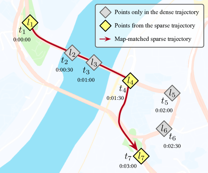
Figure 1: A sparse and a corresponding dense trajectory.

A trajectory is a sequence of timestamped locations that captures the movement of an object. In Figure 1, the travel of a vehicle from $l_{1}$ to $l_{7}$ is captured by a Trajectory $\mathcal{T}$ with seven GPS points recorded at an interval of 30 seconds: $\mathcal{T}=\langle(l_{1},t_{1}),(l_{2},t_{2}),\dots,(l_{7},t_{7})\rangle$, where $t_{i}-t_{i-1}=30$ seconds, $i\in\{2,3,\dots,7\}$. Substantial information can be mined from this trajectory, e.g., 1) the travel time of the trip, $t_{7}-t_{1}$; 2) the road segments that the trip visited; 3) the average travel speed on each road segment, which can reflect travel conditions; 4) accelerations and decelerations that capture driving behavior. Mining of such information plays an important role in enabling high-quality ITS applications.

Several excellent studies have been conducted with the goal of extracting information from spatio-temporal trajectories, employing either end-to-end [13, 14, 15] or self-supervised [16, 17, 18] methodologies. Despite the advances achieved by such methods, they generally rely on the availability of densely sampled or accurately map-matched trajectories. However, in real-world settings, trajectories are often sampled infrequently, e.g., due to the requirements of primary applications or to reduce storage requirements [19, 20]. For instance, one day of trajectories of all taxis in Chengdu, which are originally recorded at a sampling interval of 2 seconds, requires about 204.35GB of storage. By storing sparse trajectories with a sampling interval of 4 minutes, only 1.71GB of storage is needed. However, it is challenging to extract the above mentioned information from such sparse trajectories.

To illustrate, consider Figure 1, where the sparse trajectory $\mathcal{T}^{\prime}=\{(l_{1},t_{1}),(l_{4},t_{4}),(l_{7},t_{7})\}$ has a sampling interval of 90 seconds. The challenges are three fold: 1) Coarse and incomplete spatio-temporal information. In sparse trajectories, the intervals between consecutive points are enlarged, making it difficult to extract spatio-temporal information at the same detail and accuracy as for dense trajectories. For instance, in Figure 1, the vehicle decelerates between points $(l_{2},t_{2})$ and $(l_{3},t_{3})$, but this information cannot be extracted directly from the sparse trajectory. 2) Incorrect or uncertain road segment choices. Current map-matching methods either fail or yield inaccurate results when applied to sparse trajectories. In Figure 1, the sparse trajectory is map-matched incorrectly between points $(l_{4},t_{4})$ and $(l_{7},t_{7})$, due to the uncertainty caused by the sparseness. 3) Reduced effectiveness and efficiency. Sparse trajectories can be recovered to their dense counterparts using trajectory recovery methods [21, 22, 23]. Yet, this involves a two-stage scheme where additional trajectory mining methods are used to obtain information from the recovered trajectories. This scheme causes error accumulation and generally reduces the accuracy of downstream tasks, while also negatively impacting computational efficiency.

To tackle the above challenges casued by sparse trajectories, we propose an auto-regressive framework [24]. Specifically, we utilize auto-regressive generation to pre-train a model to build connections between sparse trajectories and their dense, map-matched counterparts, thus enabling the model to discern the intricate spatio-temporal information and road segment choices hidden in sparse trajectories. We also enable the model’s ability to apply to different downstream tasks while avoiding a two-stage scheme, thus enhancing the effectiveness and efficiency of the framework. We term the resulting framework General Sparse Trajectory Learning (GenSTL). The primary contributions of the paper are as follows.

• The design of an auto-regressive framework capable of extracting spatio-temporal information and road segment choices from sparse trajectories. The framework improves the performance across a variety of downstream tasks performed on sparse trajectory datasets.

• The separation of the features in trajectories into three domains to ensure flexibility, allowing application of the proposed framework to different tasks and sparse trajectories with varying sampling intervals, without relying on a two-stage scheme or a re-training procedure.

• The careful design of a feature domain encoding layer alongside a hierarchical masked trajectory encoder, facilitating the extraction of intricate information from sparse trajectories.

• A thorough experimental study on two real-world trajectory datasets and three downstream tasks, offering insight into the performance properties of the proposed framework, and providing evidence that the framework is capable of meeting it design goals.

The paper is structured as follows: Section II covers related works. Preliminary definitions and the problem statement are provided in Section III. The proposed framework is detailed in Section IV. Section V covers the experimental study, while Section VI offers concluding remarks.

II Related Work

II-A End-to-end and Self-supervised Trajectory Learning

End-to-end learning has become widely adopted for trajectory learning due to its simplicity and its ability to deliver robust performance given suitable conditions. DeepMove [1] performs trajectory prediction by using an attentional recurrent network-based trajectory encoder, followed by a fully-connected network as a predictor. HST-LSTM [2] targets the extraction of higher-level information, including functional zones, from historical trajectories. This is achieved by employing a hierarchical long-short term memory network. ACN [13] leverages convolutional filters to capture a trajectory’s local features. PreCLN [25] incorporates both spatial and road network features of a trajectory through contrastive learning, providing more comprehensive information for prediction.

While end-to-end trajectory learning approaches have their merits, they also face challenges. Key among these is the necessity for expansive, high-quality trajectory datasets to achieve satisfactory results, a requirement that may not be feasible in real-world settings. To tackle the challenges associated with end-to-end learning approaches, self-supervised methods eliminate the need for task-specific labels. Trembr [16] is a method that applies auto-encoding [26] to effectively extract road network and temporal information embedded in trajectories using self-supervised learning. SML [17] incorporates a contrastive predictive coding framework [27], offering an innovative approach to self-supervised human mobility learning. START [18] introduces a comprehensive self-supervised trajectory representation learning approach. It exploits both masked language model [28] and SimCLR [29] training tasks to enhance its learning capabilities.

While self-supervised trajectory learning techniques demonstrate versatility, enabling their application across different downstream tasks, they still rely substantially on dense, map-matched trajectory datasets to deliver optimal performance. This requirement can prove problematic, causing inaccurate results or making them infeasible when trajectories are sparse.

II-B Sparse Trajectory Recovery

Dealing with frequently encountered sparse trajectories, trajectory recovery methods aim to restore high-sampling-rate trajectories from their low-sampling-rate counterparts. Existing methods are either two-stage approaches or end-to-end approaches.

Two-stage approaches first recover “dense” GPS points and then perform map-matching. The state-of-the-art is DHTR [30], which employs a seq2seq [31] framework for GPS point recovery, supplemented by Kalman Filtering for improved robustness. The primary drawback of two-stage approaches is their sub-optimal computational efficiency and their propensity for error accumulation.

End-to-end approaches, on the other hand, recover map-matched trajectories directly in an end-to-end fashion. AttnMove [32] employs the attention mechanism to enhance human trajectories, recovering missing locations. MTrajRec [23] is a multi-task framework based on seq2seq that performs trajectory recovery and map-matching simultaneously. RNTrajRec [22] incorporates correlations between trajectories and the road network to achieve more accurate recovery results.

Although existing trajectory recovery methods have demonstrated promising performance, their use still necessitates a two-stage pipeline when integrating recovered dense trajectories in downstream tasks. This process can compromise efficiency and introduce error accumulation. Additionally, existing trajectory recovery methods offer limited generalizability across sparse trajectories with diverse sampling intervals, which reduces their applicability or effectiveness when applied to real-world trajectory datasets.

III Preliminaries

III-A Definitions

Definition 1 (Road Network).

A road network is modeled as a direct graph $\mathcal{G}=(\mathcal{V},\mathcal{E})$, where $\mathcal{V}$ is a set of nodes, each node $v_{i}\in\mathcal{V}$ models an intersection between road segments or the end of a segment, and $\mathcal{E}$ is a set of edges, where each edge $e_{i}\in\mathcal{E}$ models a road segment linking two nodes. An edge is given by starting and ending nodes: $e_{i}=(v_{j},v_{k})$.

Definition 2 (Trajectory).

A trajectory $\mathcal{T}$ is a sequence of timestamped point locations: $\mathcal{T}=\langle(l_{1},t_{1}),(l_{2},t_{2}),\dots,(l_{|\mathcal{T}|},t_{|\mathcal{T}|})\rangle$, where $l_{i}=(l^{\mathrm{lng}}_{i},l^{\mathrm{lat}}_{i})$ are the spatial coordinates of the $i$-th location, $l^{\mathrm{lng}}_{i}$ and $l^{\mathrm{lat}}_{i}$ denote longitude and latitude, respectively, and timestamp $t_{i}$ is the time at which $l_{i}$ is visited.

Definition 3 (Dense and Sparse Trajectories).

A trajectory’s sampling interval $\eta$ is the time interval between its consecutive points, i.e., $\eta=t_{i}-t_{i-1},i\in\{2,3,\dots,|\mathcal{T}|\}$. In this study, we consider dense trajectories with a sampling interval of $\eta=15$ seconds and sparse trajectories with sampling interval of $1$, $2$, and $4$ minutes. Sparse trajectories can be obtained from dense trajectories. We denote the sampling interval of a re-sampled, sparse trajectory by $\mu$.

Definition 4 (Map-matched Trajectory).

By using a map-matching algorithm [33], a trajectory $\mathcal{T}$ can be projected onto the underlying road network $\mathcal{G}$. The map-matched trajectory can be denoted as $\widetilde{\mathcal{T}}=\langle(\widetilde{l}_{1},t_{1}),(\widetilde{l}_{2},t_{2}),\dots,(\widetilde{l}_{|\mathcal{T}|},t_{|\mathcal{T}|})\rangle$, where $\widetilde{l}_{i}=(e_{i},r_{i})$, $e_{i}\in\mathcal{E}$ is the map matched road segment occupied by location $l_{i}$, and $r_{i}$ is the fraction of the length of the road segment traveled by time $t_{i}$.

Example 1.

Figure 2 gives an example of a trajectory $\mathcal{T}=\langle(l_{1},t_{1}),(l_{2},t_{2}),(l_{3},t_{3})(l_{4},t_{4})\rangle$, where the locations are denoted in diamonds. Map-matching yields map-matched trajectory $\widetilde{\mathcal{T}}=\langle(\tilde{l}_{1},t_{1}),(\tilde{l}_{2},t_{2}),(\tilde{l}_{3},t_{3}),(\tilde{l}_{4},t_{4})\rangle$, where the locations are in squares. For example, $l_{2}$ is map-matched onto $\tilde{l}_{2}$, which is in the middle of road segment $e_{2}$. Thus, we use $r_{2}$ to denote the fraction of the length of $e_{2}$ that the vehicle has traveled, resulting in $\widetilde{l}_{2}=(e_{2},r_{2})$.

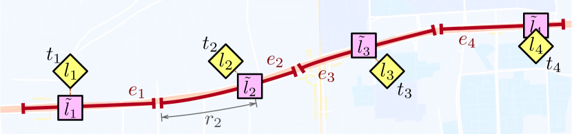
Figure 2: A trajectory and its map-matched counterpart.

Definition 5 (Tuple of Feature Domains).

Features in trajectories are split among three domains: 1) The spatial domain includes features related to spatial coordinate $l_{i}$; 2) the temporal domain refers to timestamp $t_{i}$; and 3) the road segment domain includes road segment $e_{i}$ and fraction $r_{i}$. We can transform each point in a trajectory to a tuple of these three domains. For example, point $(\tilde{l}_{i},t_{i})$ is transformed into $(l_{i},t_{i},(e_{i},r_{i}))$. A tuple transformed from the $i$-th point in trajectory $\mathcal{T}$ is denoted as $g_{i}^{\mathcal{T}}$.

III-B Problem Statement

Sparse Trajectory Learning. The objective is to construct a sparse trajectory learning model $f_{\theta}$, where $\theta$ denotes a set of learnable parameters. During evaluation, $f_{\theta}$ takes a certain arrangement of sparse trajectory $\mathcal{T}^{\prime}$ as input and outputs a result specific to a particular downstream task, denoted as $\hat{Y}=f_{\theta}(\mathrm{arrange}(\mathcal{T}^{\prime}))$. The detailed arrangement $\mathrm{arrange}(\mathcal{T}^{\prime})$ depends on the task. For example, for trajectory prediction, $\mathrm{arrange}(\mathcal{T}^{\prime})$ retains the historical part of $\mathcal{T}^{\prime}$, and $\hat{Y}$ is the predicted future part of $\mathcal{T}^{\prime}$; for travel time estimation, $\mathrm{arrange}(\mathcal{T}^{\prime})$ extracts the origin, destination, and departure time of $\mathcal{T}^{\prime}$, and $\hat{Y}$ is the estimated travel time.

IV Methodology

IV-A Overall Framework

To construct the auto-regressive framework, we draw inspiration from advancements in Natural Language Processing (NLP), specifically from the General Language Model (GLM) [34]. Take the trajectories in Figure 2 as an example. We start with a dense trajectory $\mathcal{T}=\langle(l_{1},t_{1}),(l_{2},t_{2}),(l_{3},t_{3}),(l_{4},t_{4})\rangle$, its map-matched version $\widetilde{\mathcal{T}}$, and its re-sampled, sparse counterpart $\mathcal{T}^{\prime}=\langle(l_{1},t_{1}),(l_{4},t_{4})\rangle$. Compared with $\widetilde{\mathcal{T}}$, $\mathcal{T}^{\prime}$ lacks spatio-temporal information and accurate road segment choices. We aim to pre-train a model $f_{\theta}$ to generate $\widetilde{\mathcal{T}}$ from $\mathcal{T}^{\prime}$. This way, the model builds the connection between a sparse trajectory and its dense, map-matched counterpart.

A representation of the proposed framework is shown in Figure 3. Each point in a trajectory is first transformed into a tuple of feature domains following Definition 5. Tuples with feature domains missing in $\mathcal{T}^{\prime}$ but present in $\widetilde{\mathcal{T}}$ need to be generated. Especially, the two tuples $g_{2}^{\widetilde{\mathcal{T}}}$ and $g_{3}^{\widetilde{\mathcal{T}}}$ are missing in $\mathcal{T}^{\prime}$. To explicitly mark these missing tuples, we replace any consecutive missing tuples with a special mask tuple $g_{[m]}=([m],[m],[m])$. The resulting sequence, which we call an input sparse trajectory, is formulated as $\mathcal{T}^{(\mathrm{in})}=\langle g_{1}^{\mathcal{T}^{\prime}},g_{[m]},g_{2}^{\mathcal{T}^{\prime}}\rangle$.

Each tuple in $\mathcal{T}^{(\mathrm{in})}$ corresponds to a part of $\widetilde{\mathcal{T}}$ that needs to be generated. In Figure 3, $g_{1}^{\mathcal{T}^{\prime}}$ corresponds to $\langle g_{1}^{\widetilde{\mathcal{T}}}\rangle$, $g_{[m]}$ corresponds to $\langle g_{2}^{\widetilde{\mathcal{T}}},g_{3}^{\widetilde{\mathcal{T}}}\rangle$, and $g_{2}^{\mathcal{T}^{\prime}}$ corresponds to $\langle g_{4}^{\widetilde{\mathcal{T}}}\rangle$. We denote each of these parts as a span. To guide the encoder to generate each span auto-regressively, we follow common practice and construct a pair of source and target spans. Specifically, each span is prepended with one start tuple $g_{[s]}=([s],[s],[s])$ as the input source span, and is appended with one end tuple $g_{[e]}=([e],[e],[e])$ as the output target span. The source and target spans constructed from all spans in $\widetilde{\mathcal{T}}$ are concatenated to form the source sequence $\mathcal{T}^{(\mathrm{src})}$ and the target dense trajectory $\mathcal{T}^{(\mathrm{tgt})}$. Since auto-regression is uni-directional, to retain the learning model’s ability to extract bi-directional correlations, the pairs of source and target spans undergo random shuffling before concatenation.

Two layers of positions are associated with $\mathcal{T}^{(\mathrm{in})}$ and $\mathcal{T}^{(\mathrm{src})}$. The first layer denotes the positions of tuples of $\mathcal{T}^{(\mathrm{in})}$ and source spans of $\mathcal{T}^{(\mathrm{src})}$. The second layer denotes the positions of tuples within each source spans of $\mathcal{T}^{(\mathrm{src})}$.

Finally, $\mathcal{T}^{(\mathrm{in})}$ is fed into the model as known information, $\mathcal{T}^{(\mathrm{src})}$ is provided as a guide for the auto-regressive generation, and $\mathcal{T}^{(\mathrm{tgt})}$ is the label of the generation. The two layers of positions are also fed as input. More preparation details of these sequences are provided in Section IV-B. Our model $f_{\theta}$ is implemented with a feature domain encoding layer and a hierarchical masked trajectory encoder, whose designs are presented in Sections IV-C and IV-D. A comprehensive explanation of the pre-training and the downstream adaptation is provided in Section IV-E.

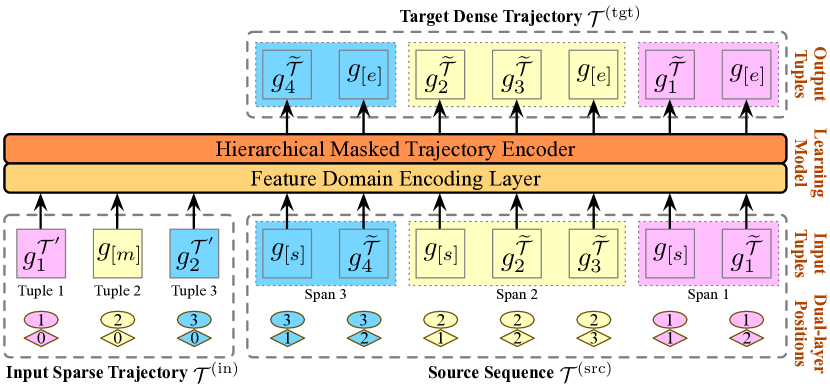
Figure 3: Overall framework.

IV-B Construction of Input and Output Sequences

IV-B1 Sparse Trajectory Resampling

Initially, a dense trajectory $\mathcal{T}\in\mathbb{T}$ is selected from the dataset, where its sampling interval $\eta$ is no longer than 15 seconds. To extract its road segment-related information, the Fast Map Matching (FMM) algorithm [35] is applied, as shown next.

$$\widetilde{\mathcal{T}}=\mathrm{FMM}(\mathcal{T},\mathcal{G})=\langle(\tilde{l}_{1},t_{1}),(\tilde{l}_{2},t_{2}),\dots,(\tilde{l}_{|\mathcal{T}|},t_{|\mathcal{T}|})\rangle$$ (1)

Simultaneously, to emulate sparse trajectories with long sampling intervals, $\mathcal{T}$ is resampled at a interval $\mu$, where $\mu>\eta$ and $\mu$ is divisible by $\eta$, to derive a sparse counterpart of $\mathcal{T}$. This process is formulates as follows.

Notice that the last trajectory point in $\mathcal{T}$ is retained in $\mathcal{T}^{\prime}$ to maintain the integrity of the re-sampled trajectory.

Each trajectory point in $\mathcal{T}^{\prime}$ is present in $\widetilde{\mathcal{T}}$. However, compared to the point $(\tilde{l}_{i},t_{i})$ in $\widetilde{\mathcal{T}}$, the point $(l_{i},t_{i})$ in $\mathcal{T}^{\prime}$ lacks the road segment domain. We use a special token $[m]$ to denote the absence of this domain and transform the $i$-th point of $\mathcal{T}^{\prime}$ into a tuple following Definition 5:

$$g_{i}^{\mathcal{T}^{\prime}}=((l_{j},\Omega(l_{j})),t_{j},[m]),j=1+(i-1)\mu/\eta$$ (3)

Here, $t_{j}$ is the normalized time of the day, and $\Omega(l_{j})$ that represents the set of road segment neighbors associated with coordinate $l_{j}$ is added to the spatial domain of this tuple. This enhances the framework’s understanding of the relationship between spatial coordinates and the road segment. Formally:

$$\Omega(l_{i})=\{e_{j},e_{j}\in\mathcal{E},\mathrm{dist}(l_{i},e_{j})\leqslant\delta\},$$ (4)

where $\mathrm{dist}$ measures the shortest distance between a coordinate and the center of a road segment on the Earth’s surface, and $\delta$ is a distance threshold in meters and is an tunable hyper-parameter.

Sub-trajectories of $\widetilde{\mathcal{T}}$ that fall between consecutive points in $\mathcal{T}^{\prime}$ are absent from $\mathcal{T}^{\prime}$. We use a special tuple $g_{[m]}=([m],[m],[m])$ to denote the absence of each such sub-trajectory. This tuple is inserted between pairs of normal tuples $g_{i}^{\mathcal{T}^{\prime}}$ and $g_{i+1}^{\mathcal{T}^{\prime}}$.

Finally, the input sparse trajectory $\mathcal{T}^{(\mathrm{in})}$ is constructed as a sequence of tuples:

$$\mathcal{T}^{(\mathrm{in})}=\langle g_{1}^{\mathcal{T}^{\prime}},g_{[m]},g_{2}^{\mathcal{T}^{\prime}},g_{[m]},\dots,g_{|\mathcal{T}^{\prime}|}^{\mathcal{T}^{\prime}}\rangle$$ (5)

IV-B2 Source and Target Pairs

Each normal tuple $g_{i}^{\mathcal{T}^{\prime}}$ corresponds to the $j$-th trajectory point $(\tilde{l}_{j},t_{j})$ in $\widetilde{\mathcal{T}}$, where $j=1+(i-1)\mu/\eta$. Point $(\tilde{l}_{j},t_{j})$ needs to be generated during pre-training. We can transform this point into a span with a single tuple following Definition 5:

$$\langle g_{j}^{\widetilde{\mathcal{T}}}\rangle=\langle(l_{j},t_{j},(e_{j},r_{j}))\rangle$$ (6)

In Figure 3, the tuple $g_{1}^{\mathcal{T}^{\prime}}$ corresponds to the span $\langle g_{1}^{\widetilde{\mathcal{T}}}\rangle$, and the tuple $g_{2}^{\mathcal{T}^{\prime}}$ corresponds to the span $\langle g_{4}^{\widetilde{\mathcal{T}}}\rangle$.

On the other hand, each special tuple $g_{[m]}$ corresponds to a sub-trajectory of $\widetilde{\mathcal{T}}$ that also needs to be generated. We can transform each point in the sub-trajectory similar to Equation 6 and obtain a span with one or multiple tuples. In Figure 3, the tuple $g_{[m]}$ corresponds to the span $\langle g_{2}^{\widetilde{\mathcal{T}}},g_{3}^{\widetilde{\mathcal{T}}}\rangle$.

To enable auto-regressive generation of these spans, we construct a pair of source and target spans for each span to be generated. Specifically, given a span $\langle g_{j}^{\widetilde{\mathcal{T}}}\rangle$, a special tuple $g_{[s]}=([s],[s],[s])$ is prepended to form the source span $\langle g_{[s]},g_{j}^{\widetilde{\mathcal{T}}}\rangle$, and a special tuple $g_{[e]}=([e],[e],[e])$ is appended to form the target span $\langle g_{j}^{\widetilde{\mathcal{T}}},g_{[e]}\rangle$. This process generalizes to scenarios where a span with multiple tuples is given. We use $g_{[s]}$ to denote the start of a span, and $g_{[e]}$ to denote the end of one.

Having constructed all pairs of source and target spans, their ordering undergoes a random permutation to enable the model’s bi-directional extraction of correlations. The source sequence $\mathcal{T}^{(\mathrm{src})}$ and the target dense trajectory $\mathcal{T}^{(\mathrm{tgt})}$ are then concatenated by the permuted source and target spans, respectively. In Figure 3, $\mathcal{T}^{(\mathrm{src})}$ and $\mathcal{T}^{(\mathrm{tgt})}$ are concatenated by the source and target spans corresponding to the spans to be generated: $\langle g_{4}^{\widetilde{\mathcal{T}}}\rangle$, $\langle g_{2}^{\widetilde{\mathcal{T}}},g_{3}^{\widetilde{\mathcal{T}}}\rangle$, and $\langle g_{1}^{\widetilde{\mathcal{T}}}\rangle$.

IV-B3 Dual-layer Positions

Since each tuple in $\mathcal{T}^{(\mathrm{in})}$ corresponds to one span in $\mathcal{T}^{(\mathrm{src})}$, following the practice of GLMs [34], we employ dual-layer positions.

The first layer of positions signifies the correspondence between tuples in $\mathcal{T}^{(\mathrm{in})}$ and spans in $\mathcal{T}^{(\mathrm{src})}$. Specifically, the first layer of positions for the $i$-th tuple of $\mathcal{T}^{(\mathrm{in})}$ and the $i$-th span of $\mathcal{T}^{(\mathrm{src})}$ is computed as follows.

$$\mathcal{P}^{1,(\mathrm{in})}_{i}=i,\mathcal{P}^{1,(\mathrm{src})}_{i}=\langle i,i,\dots,i\rangle$$ (7)

The second layer of positions represents the order of tuples within each span of $\mathcal{T}^{(\mathrm{src})}$. Thus, the second layer of positions for the $i$-th tuple of $\mathcal{T}^{(\mathrm{in})}$ and the $i$-th span of $\mathcal{T}^{(\mathrm{src})}$ is calculated as follows.

$$\mathcal{P}^{2,(\mathrm{in})}_{i}=0,\mathcal{P}^{2,(\mathrm{src})}_{i}=\langle 1,2,\dots,N\rangle,$$ (8)

where $N$ is the length of the $i$-th span of $\mathcal{T}^{(\mathrm{src})}$.

IV-C Feature Domain Encoding

The three feature domains in each tuple include both continuous numerical and discrete categorical features. We propose a carefully designed feature domain encoding layer to enhance the model’s ability to extract information from these domains. This layer is used to cast domains of features into the latent space. Figure 4 presents an overview of the layer, where the three domains are colored blue, green, and red.

IV-C1 Encoding Continuous Numerical Features

Continuous features often exhibit periodic characteristics. For example, a driver’s travel behavior tends to exhibit similarities during the same periods of the day or days of the week. Further, the relative distance between two trajectory points’ continuous features can reveal high-level information, such as the travel distance and time between two points.

To mirror these characteristics of continuous features, we design the continuous numerical feature encoding module by drawing inspiration from Learnable Fourier Features [36, 37]. Given an input numerical feature $x\in\mathbb{R}$, the encoding module $\varPhi$ projects it onto a $d$-dimensional latent space, defined as follows.

$$\begin{split}\varPhi:\mathbb{R}\rightarrow\mathbb{R}^{d},\varPhi(x)&=\boldsymbol{W}_{\varPhi}[\cos(x\boldsymbol{v}_{\varPhi})\|\sin(x\boldsymbol{v}_{\varPhi})]\\ x&\in\{l_{i}^{\mathrm{lng}},l_{i}^{\mathrm{lat}},t_{i},r_{i}\},\end{split}$$ (9)

where $\boldsymbol{v}_{\varPhi}\in\mathbb{R}^{d/2}$ represents a learnable projection vector, and $\boldsymbol{W}_{\varPhi}\in\mathbb{R}^{d\times d}$ denotes a learnable projection matrix. Importantly, distinct sets of $\boldsymbol{v}_{\varPhi}$ and $\boldsymbol{W}_{\varPhi}$ are utilized for the four types of numerical features.

With $\varPhi$, the input features’ periodic characteristics are retained due to the inherent properties of trigonometric functions. Meanwhile, given that $\cos x_{1}\cos x_{2}+\sin x_{1}\sin x_{2}=\cos(x_{1}-x_{2})$, and considering that the distances between latent vectors are typically calculated using the dot-product, $\varPhi$ amplifies the model’s ability to discern the relative distances between features. This is evidenced by the dot-product between two encoding vectors $\varPhi(x_{1})$ and $\varPhi(x_{2})$:

$$\varPhi(x_{1})\cdot\varPhi(x_{2})=\|\boldsymbol{W}_{\varPhi}\|_{2}\cos(x_{1}-x_{2})\|\boldsymbol{v}_{\varPhi}\|_{1},$$ (10)

which means the distance between the encoding vectors of two values hinges solely on the learnable parameters and the relative difference between the two values.

IV-C2 Embedding Discrete Indices and Tokens

An index-fetching embedding module is utilized to project the discrete road segment indices in $\mathcal{T}^{(\mathrm{src})}$ into the latent space. The module consists of a learnable matrix $\boldsymbol{E}_{\mathcal{E}}\in\mathbb{R}^{|\mathcal{E}|\times d}$. The embedding vector of road segment $s_{i}$ is obtained as the $s_{i}$-th row vector of $\boldsymbol{E}_{\mathcal{E}}$, denoted as $\boldsymbol{E}_{\mathcal{E}}(s_{i})$.

Likewise, for segment indices in the neighbor set $\Omega(l_{i})$, another embedding module with matrix $\boldsymbol{E}_{\Omega}\in\mathbb{R}^{|\mathcal{E}|\times d}$ is used to fetch one embedding vector for each road segment within the set. The set of embeddings of road segments in $\Omega(l_{i})$ is represented by $\Omega_{E}(l_{i})=\{\boldsymbol{E}_{\Omega}(s_{j}),s_{j}\in\Omega(l_{i})\}$.

Considering next the special tokens $\{[m],[s],[e]\}$, one embedding vector is designated for each token within each domain, resulting in a total of 9 embedding vectors. These vectors are combined to form a matrix $\boldsymbol{E}_{\mathrm{token}}\in\mathbb{R}^{9\times d}$:

$$\boldsymbol{E}_{\mathrm{token}}=\|_{i\in\{[m],[s],[e]\}}[\boldsymbol{e}^{\mathrm{sp}}_{i},\boldsymbol{e}^{\mathrm{te}}_{i},\boldsymbol{e}^{\mathrm{rn}}_{i}],$$ (11)

where $\boldsymbol{e}^{\mathrm{sp}}_{i}$, $\boldsymbol{e}^{\mathrm{te}}_{i}$, and $\boldsymbol{e}^{\mathrm{rn}}_{i}$ are the embedding vectors for a specific token in spatial, temporal, and road network domains, respectively.

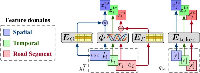
Figure 4: The feature domain encoding layer.

IV-C3 Fusing Encoding and Embedding Vectors

The encoding vectors of continuous numerical features and the embedding vectors of discrete indices and tokens are gathered to generate a tuple of latent vectors for each tuple in $\mathcal{T}^{(\mathrm{in})}$ and $\mathcal{T}^{(\mathrm{src})}$.

For a given tuple $((l_{i},\Omega(l_{i})),t_{i},(e_{i},r_{i}))$, the latent vectors for the spatial, temporal, and road network domains are calculated as follows.

$$\begin{split}{\boldsymbol{z}^{\prime}}^{\mathrm{sp}}_{i}&=\varPhi(l_{i}^{\mathrm{lng}})+\varPhi(l_{i}^{\mathrm{lat}})\\ \boldsymbol{z}^{\mathrm{sp}}_{i}&={\boldsymbol{z}^{\prime}}^{\mathrm{sp}}_{i}+\mathrm{MultiHead}({\boldsymbol{z}^{\prime}}^{\mathrm{sp}}_{i},\Omega_{E}(l_{i}),\Omega_{E}(l_{i}))\\ \boldsymbol{z}^{\mathrm{te}}_{i}&=\varPhi(t_{i})\\ \boldsymbol{z}^{\mathrm{rn}}_{i}&=\boldsymbol{E}_{\mathcal{E}}(s_{i})+\varPhi(r_{i})\end{split}$$ (12)

Here, $\mathrm{MultiHead}$ represents the dot-product attention defined in the transformer [38], with $N_{h}$ attention heads. In scenarios where any feature domain is one of the special tokens, the latent vector of that domain is substituted with the embedding vector of the corresponding special token. For tuples in $\mathcal{T}^{(\mathrm{src})}$, since the neighbor set $\Omega(l_{i})$ is missing, ${\boldsymbol{z}^{\prime}}^{\mathrm{sp}}_{i}$ is treated as the final latent vector $\boldsymbol{z}^{\mathrm{sp}}_{i}$.

Finally, the tuple of latent vectors is expressed as follows.

$$\boldsymbol{Z}_{i}=(\boldsymbol{z}^{\mathrm{sp}}_{i},\boldsymbol{z}^{\mathrm{te}}_{i},\boldsymbol{z}^{\mathrm{rn}}_{i})$$ (13)

IV-D Hierarchical Masked Trajectory Encoder

We propose a hierarchical masked trajectory encoder to model the correlations between the tuples in $\mathcal{T}^{(\mathrm{in})}$ and $\mathcal{T}^{(\mathrm{src})}$ and to auto-regressively generate $\mathcal{T}^{(\mathrm{tgt})}$. The architecture of the encoder is shown in Figure 5.

In accordance with Equation 13, each tuple in $\mathcal{T}^{(\mathrm{in})}$ and $\mathcal{T}^{(\mathrm{src})}$ is represented by a latent tuple, which contains three latent vectors that represent the three feature domains. To understand the interrelationships between the different domains in a tuple, the following tuple-level self-attention mechanism is used.

$$(\boldsymbol{h}^{\mathrm{sp}}_{i},\boldsymbol{h}^{\mathrm{te}}_{i},\boldsymbol{h}^{\mathrm{rn}}_{i})=\mathrm{MultiHead}(\boldsymbol{Z}_{i},\boldsymbol{Z}_{i},\boldsymbol{Z}_{i})$$ (14)

During calculation, $\boldsymbol{Z}_{i}$ is treated as a sequence of length 3. Subsequently, the hidden state of this tuple is acquired by applying a tuple-wise mean pooling, followed by the position encoding of the dual-layer positions defined in Equations 7 and 8, formulated as follows.

$$\boldsymbol{h}_{i}=\mathrm{Mean}(\boldsymbol{h}^{\mathrm{sp}}_{i},\boldsymbol{h}^{\mathrm{te}}_{i},\boldsymbol{h}^{\mathrm{rn}}_{i})+\mathrm{PE}(\mathcal{P}^{1}_{i})+\mathrm{PE}(\mathcal{P}^{2}_{i}),$$ (15)

where $\mathrm{PE}$ represents the positional encoding from the transformer [38].

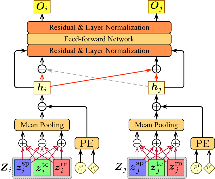
Figure 5: The hierarchical masked trajectory encoder.

Upon applying Equation 15 to each tuple in $\mathcal{T}^{(\mathrm{in})}$ and $\mathcal{T}^{(\mathrm{src})}$, we obtain two sequences of hidden states:

$$\begin{split}\boldsymbol{H}^{(\mathrm{in})}&=\langle\boldsymbol{h}_{1}^{(\mathrm{in})},\boldsymbol{h}_{2}^{(\mathrm{in})},\dots,\boldsymbol{h}_{|\mathcal{T}^{(\mathrm{in})}|}^{(\mathrm{in})}\rangle\\ \boldsymbol{H}^{(\mathrm{src})}&=\langle\boldsymbol{h}_{1}^{(\mathrm{src})},\boldsymbol{h}_{2}^{(\mathrm{src})},\dots,\boldsymbol{h}_{|\mathcal{T}^{(\mathrm{src})}|}^{(\mathrm{src})}\rangle\\ \end{split}$$ (16)

To extract information from $\boldsymbol{H}^{(\mathrm{in})}$ and simultaneously implement the auto-regressive generation of $\mathcal{T}^{(\mathrm{tgt})}$, we employ a sequence-level self-attention with a casual mask. This attention calculation is formulated as follows.

$$\begin{split}\boldsymbol{H}^{{}^{\prime}(\mathrm{in})}\|\boldsymbol{H}^{{}^{\prime}(\mathrm{src})}&=\mathrm{MultiHead}(\boldsymbol{H},\boldsymbol{H},\boldsymbol{H},\boldsymbol{M})\\ \boldsymbol{H}&=\boldsymbol{H}^{(\mathrm{in})}\|\boldsymbol{H}^{(\mathrm{src})}\end{split}$$ (17)

The attention mask $\boldsymbol{M}\in\mathbb{R}^{|\boldsymbol{H}|\times|\boldsymbol{H}|}$ ensures that every step in $\boldsymbol{H}^{(\mathrm{in})}$ can be attended by any step in $\boldsymbol{H}$, while every step in $\boldsymbol{H}^{(\mathrm{src})}$ can only be attended by itself and its predecessors. Specifically, each element of the mask is calculated as follows.

$$\boldsymbol{M}_{i,j}=\left\{\begin{array}[]{ll}\mathrm{True}&\mathrm{if}~{}j>|\boldsymbol{H}^{(\mathrm{in})}|~{}\mathrm{and}~{}i<j\\ \mathrm{False}&\mathrm{otherwise}\end{array}\right.$$ (18)

Adhering to the design of the transformer encoder [38], the output state of our trajectory encoder combines $\boldsymbol{H}^{{}^{\prime}(\mathrm{src})}$ derived from Equation 17 with residual connections, layer normalization, and a feed-forward network. This is expressed as follows.

$$\begin{split}\boldsymbol{O}^{\prime}&=\mathrm{LayerNorm}(\boldsymbol{H}^{{}^{\prime}(\mathrm{src})}+\boldsymbol{H}^{(\mathrm{src})})\\ \boldsymbol{O}&=\mathrm{LayerNorm}(\mathrm{FFN}(\boldsymbol{O}^{\prime})+\boldsymbol{O}^{\prime}),\end{split}$$ (19)

where $\boldsymbol{O}$ represents the output state and $\mathrm{FFN}$ is the feed-forward network composed of two fully connected layers.

Lastly, the prediction of the target dense trajectory $\mathcal{T}^{(\mathrm{tgt})}$ is obtained using four prediction modules, tasked with predicting coordinates $l_{i}$, time $t_{i}$, road segment $s_{i}$, and the travel fraction $r_{i}$. Formally, the prediction on the feature domains of the $i$-th tuple in $\mathcal{T}^{(\mathrm{tgt})}$ is calculated as follows.

$$\begin{split}\hat{l_{i}}&=\boldsymbol{W}_{c}\boldsymbol{O}_{i}+\boldsymbol{b}_{c}\\ \hat{t_{i}}&=\boldsymbol{W}_{t}\boldsymbol{O}_{i}+\boldsymbol{b}_{t}\\ \hat{s_{i}}&=\operatorname*{argmax}(p(\hat{s_{i}})),~{}p(\hat{s_{i}})=\mathrm{Softmax}(\boldsymbol{W}_{s}\boldsymbol{O}_{i}+\boldsymbol{b}_{s})\\ \hat{r_{i}}&=\boldsymbol{W}_{r}\boldsymbol{O}_{i}+\boldsymbol{b}_{r},\end{split}$$ (20)

where $\boldsymbol{W}_{c}\in\mathbb{R}^{2\times d}$, $\boldsymbol{W}_{t}\in\mathbb{R}^{1\times d}$, $\boldsymbol{W}_{s}\in\mathbb{R}^{(|\mathcal{E}|+1)\times d}$, and $\boldsymbol{W}_{r}\in\mathbb{R}^{1\times d}$ denote the projection matrices, while $\boldsymbol{b}_{c}\in\mathbb{R}^{2}$, $\boldsymbol{b}_{t}\in\mathbb{R}^{1}$, $\boldsymbol{b}_{s}\in\mathbb{R}^{(|\mathcal{E}|+1)}$, and $\boldsymbol{b}_{r}\in\mathbb{R}^{1}$ are biases. The predicted road segment index $\hat{s_{i}}\in\mathcal{E}\cup\{[e]\}$ also functions as an end token indicator.

IV-E Pre-training

Initially, the proposed framework undergoes pre-training on sequences that are prepared according to the scheme detailed in Section IV-B. Subsequently, it is adapted for specific downstream tasks with input arrangements tailored to the particular task.

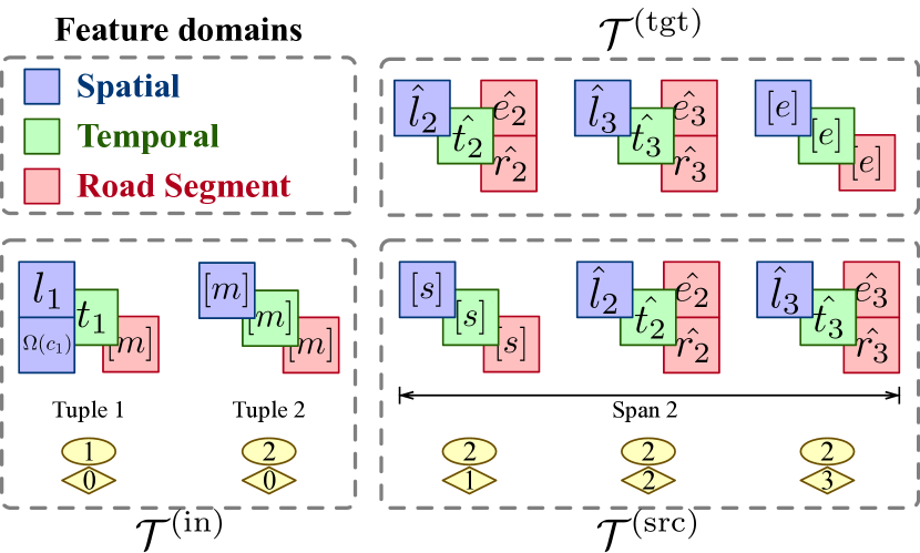
(a) Trajectory Prediction

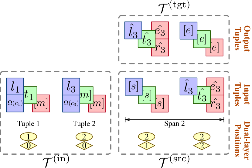
(b) Travel Time Estimation

Figure 6: Unique input and target arrangements for different downstream tasks.

IV-E1 Pre-training Loss

For a given training sample $(\mathcal{T}^{(\mathrm{in})},\mathcal{T}^{(\mathrm{src})},\mathcal{T}^{(\mathrm{tgt})})$, the pre-training loss is computed based on the generated $\widehat{\mathcal{T}}^{(\mathrm{tgt})}$, where $\mathcal{T}^{(\mathrm{tgt})}$ is the generation label. The loss for the $i$-th tuple is computed as follows.

where $\mathbbm{1}^{[e]}_{i}$ indicates whether the $i$-th tuple is an end tuple, and is computed as follows.

$$\mathbbm{1}^{[e]}_{i}=\left\{\begin{array}[]{ll}0&\mathrm{if}~{}\mathcal{T}^{(\mathrm{tgt})}_{i}=g_{[e]}\\ 1&\mathrm{otherwise}\end{array}\right.$$ (22)

The overall pre-training loss for the sample is then the mean of losses across the entire target dense trajectory:

$$\mathcal{L}_{\mathcal{T}^{(\mathrm{tgt})}}=\frac{1}{|\mathcal{T}^{(\mathrm{tgt})}|}\sum_{i=1}^{|\mathcal{T}^{(\mathrm{tgt})}|}\mathcal{L}_{i}$$ (23)

IV-E2 Pre-training Procedure

Given a trajectory dataset $\mathbb{T}$, we construct a training set $\mathbb{T}^{\prime}$ by selecting trajectories with sampling intervals that fall below a predefined threshold, which is set at 15 seconds in our case. For every trajectory $\mathcal{T}\in\mathbb{T}^{\prime}$, a variety of re-sampling intervals are employed to generate multiple sets of pre-training samples. This procedure is expressed as follows.

$$\Lambda_{\mathcal{T}}=\bigcup_{\mu\in\Gamma}(\mathcal{T}^{(\mathrm{in})},\mathcal{T}^{(\mathrm{src})},\mathcal{T}^{(\mathrm{tgt})}),$$ (24)

where $\Lambda_{\mathcal{T}}$ is the aggregated set of pre-training samples derived from trajectory $\mathcal{T}$ and $\Gamma$ is a set of re-sampling intervals, i.e., $\Gamma=\{1~{}\mathrm{minute},2~{}\mathrm{minutes},4~{}\mathrm{minutes}\}$ in our configuration. The optimization objective during the pre-training of our proposed framework is defined as follows.

$$\operatorname*{argmax}_{\theta}\sum_{\mathcal{T}\in\mathbb{T}^{\prime}}\sum_{\mathcal{T}^{(\mathrm{tgt})}\in\Lambda_{\mathcal{T}}}-\mathcal{L}_{\mathcal{T}^{(\mathrm{tgt})}},$$ (25)

By pre-training on simulated sparse trajectories across diverse re-sampling intervals, we can enhance the versatility and generalization capabilities of the proposed framework.

IV-F Adaptation to Downstream Tasks

The flexibility of the framework enables its transferability to a wide range of downstream tasks after pre-training. This section details the input arrangements required for three distinct downstream tasks.

IV-F1 Sparse Trajectory Recovery (STR)

This task involves the input and output sequences defined in Section IV-B. The only difference is that the spans in $\mathcal{T}^{(\mathrm{src})}$ and $\mathcal{T}^{(\mathrm{tgt})}$ do not need to be shuffled. Whether spans between consecutive points are absent in a sparse trajectory can be deduced from the sampling interval. Specifically, suppose we have trajectory points $(l_{i},t_{i})$ and $(l_{i+1},t_{i+1})$ and a given desired sampling interval $\eta$. If $t_{i+1}-t_{i}>\eta$ then we insert a mask tuple $g_{[m]}$ between these two points, indicating that there is an absent span to be recovered.

IV-F2 Trajectory Prediction (TP)

This task aims to predict future trajectory points given historical ones. Suppose we have a historical sparse trajectory $\mathcal{T}^{\prime}=\langle(l_{1},t_{1}),(l_{2},t_{2}),\dots,(l_{n},t_{n})\rangle$. A corresponding input sparse trajectory:

is provided to the framework. The source sequence begins with a single start tuple, i.e., $\mathcal{T}^{(\mathrm{src})}=\langle([s],[s],[s])\rangle$, and the framework generates the prediction of the future tuple-by-tuple in an auto-regressive manner, until the predicted road segment is the end token, that is, $\arg\max p(\hat{s_{i}})=[e]$. Figure 6(a) provides an example arrangement.

IV-F3 Travel Time Estimation (TTE)

This task involves estimating the travel time of a sparse trajectory given only the origin-destination location pair and the departure time. Given the the origin and destination locations and the departure time of a sparse trajectory, $l_{1}$, $l_{N}$, and $t_{1}$, the input sparse trajectory is constructed as follows.

$$\mathcal{T}^{(\mathrm{in})}=\langle g_{1}^{\mathcal{T}^{\prime}},g_{N}^{\mathcal{T}^{\prime}}\rangle=\langle(l_{1},t_{1},[m]),(l_{N},[m],[m])\rangle,$$ (27)

as illustrated in Figure 6(b). Since the estimated time $\hat{t_{i}}$ is designed to be a temporal offset with regard to the first trajectory point, the time of the last point in the generated trajectory $\widehat{\mathcal{T}}^{(\mathrm{tgt})}$ is the estimated travel time.

V Experiments

To access the performance of the proposed framework, we conduct experiments on two real-world trajectory datasets under varying experimental settings.

V-A Datasets

We use two datasets for experiments, comprising taxi trajectories from Chengdu, China, and Porto, Portugal. For consistency in our analyses, these datasets, which we call Chengdu and Porto, are both standardized to a sampling interval of 15 seconds. Trajectories that feature fewer than 6 points, being relatively short, are excluded from our study. An overview of dataset statistics can be found in Table I.

TABLE I: Dataset statistics.

Dataset	Chengdu	Porto
Time span	10.01–11.30, 2018	07.01–09.01, 2013
Longitude scope	104.04300$\sim$104.12654	-8.65200$\sim$-8.57801
Latitude scope	30.65523$\sim$30.72699	41.14201$\sim$41.17399
Number of road segments	2,505	2,225
Number of trajectories	121,394	55,120
Number of points	3,032,212	1,482,751

V-B Comparison Methods

To assess the performance of the proposed framework across the three downstream tasks outlined in Section IV-F, we benchmark its performance against a variety of state-of-the-art methods, each specialized for a particular task.

V-B1 Sparse Trajectory Recovery Methods

We compare the proposed framework on the STR task against the following state-of-the-art sparse trajectory recovery methods.

• Shortest Path [39]: recovers paths between consecutive points in sparse trajectories with Dijkstra’s shortest path algorithm [40] on road networks.

• Linear [41]+HMM [42]: extends sparse trajectories using linear interpolation, then applies the HMM algorithm.

• TrImpute [21]+HMM: imputes sparse trajectories with a crowd wisdom-based algorithm.

• DHTR [30]+HMM: combines seq2seq [31], Kalman filtering, and the HMM algorithm to recover dense trajectories.

• AttnMove [32]: leverages Attention mechanisms to predict the sequence of road segments.

• MTrajRec [23]: employs a GRU-based auto-regressive model to recover road network-constrained trajectories.

• RNTrajRec [22]: integrates the transformer model and the inherent road network structure to recover trajectories.

V-B2 Trajectory Prediction Methods

We have selected several trajectory prediction methods, both end-to-end and self-supervised, for comparison.

• trajectory2vec [43]: constructs behavior sequences to extract high-level correlations in trajectories.

• t2vec [44]: builds upon an auto-encoding framework, offering a more robust self-supervised trajectory learning model.

• DeepMove [1]: an end-to-end Attentional RNN-based sequential model designed for predicting future movements.

• Transformer [38]: a widely-used sequential model that excels at extracting correlations in long sequences.

• Trembr [16]: integrates road network information with auto-encoding for self-supervised trajectory learning.

• START [18]: incorporates both spatio-temporal correlations and travel semantics for self-supervised learning.

It is noteworthy that Trembr and START require map-matched trajectories for optimal functioning, which are not directly obtainable in the context of sparse trajectories. Therefore, the trajectories recovered by the most effective STR baseline, RNTrajRec, are served as input to them during evaluation. These combinations are denoted as Trembr+RNTR and START+RNTR. We also report their performance when they are fed with map-matched, real dense trajectories.

V-B3 Travel Time Estimation Methods

In the TTE task, the only provided information is the origin, destination, and departure time. We therefore benchmark the performance of the proposed framework against OD travel time estimation methods that operate under analogous conditions.

• RNE [45]: determines the path distances between road segments by referencing their latent embeddings.

• TEMP [46]: calculates the mean travel times of historical trajectories that align closely in terms of locations and time.

• LR: establishes a linear mapping from input features to travel times based on training labels.

• GBM: an advances non-linear regression model, which we implement via XGBoost [47].

• ST-NN [48]: concurrently predicts both travel distances and travel times for OD pairs.

• MURAT [49]: jointly predicts travel distance and time while utilizing the departure time as extra information.

• DeepOD [5]: exploits the correlation between input features and historical trajectories during training.

• DOT [50]: a two-stage framework that generates an image representation of trajectories for estimating travel time.

V-B4 Variations without pre-training or fine-tuning

To further assess the effectiveness of the pre-training and fine-tuning processes within the proposed framework, we introduce two additional variations for comparison.

• GenSTL w/o pt: excludes the pre-training process, training the framework solely with task-specific data.

• GenSTL w/o ft: bypasses the fine-tuning process, enabling the framework to undertake downstream tasks immediately after pre-training with task-specific input arrangements.

V-C Settings

TABLE II: Hyper-parameter range and optimal values.

Parameter	Range
$d$	32, 64, 128, 192, 256
$N_{h}$	1, 2, 4, 8, 16
$\delta$ (meters)	10, 50, 100, 150, 200

TABLE III: Sparse Trajectory Recovery accuracy comparison of different approaches.

Sampling Interval $\mu$		1 minute / 2 minutes / 4 minutes
Datasets	Methods	Precision (%)	Recall (%)	MAE (Coor, meters)	MAE (Road, meters)
Chengdu	Shortest Path	62.638 / 43.504 / 29.431	59.346 / 40.949 / 27.607	213.10 / 428.69 / 752.19	206.91 / 391.39 / 586.09
	Linear+HMM	66.642 / 48.604 / 36.209	65.557 / 45.234 / 30.496	183.64 / 385.23 / 675.85	169.46 / 378.96 / 564.19
	TrImpute+HMM	77.520 / 60.179 / 57.526	76.202 / 58.461 / 53.747	166.82 / 276.56 / 408.64	155.71 / 265.34 / 387.36
	DHTR+HMM	53.514 / 53.608 / 50.985	58.868 / 47.918 / 46.311	205.59 / 317.45 / 450.61	300.67 / 470.46 / 547.41
	AttnMove	84.162 / 81.402 / 78.645	81.839 / 76.612 / 69.257	252.59 / 280.20 / 354.39	201.51 / 258.69 / 323.52
	MTrajRec	85.039 / 82.596 / 80.684	83.351 / 80.113 / 72.952	243.01 / 264.15 / 311.53	173.67 / 204.58 / 282.88
	RNTrajRec	87.653 / 83.174 / 79.404	86.025 / 80.150 / 72.633	215.24 / 234.27 / 326.92	114.04 / 148.04 / 292.61
	GenSTL w/o pt	83.720 / 77.425 / 72.471	82.827 / 73.933 / 62.757	194.30 / 272.86 / 479.49	86.15 / 230.68 / 448.98
	GenSTL w/o ft	87.664 / 83.592 / 79.096	85.837 / 78.406 / 70.717	137.69 / 217.85 / 350.29	81.81 / 167.16 / 315.07
	GenSTL	89.071 / 84.373 / 80.828	88.249 / 81.520 / 73.212	133.38 / 192.54 / 304.72	67.98 / 143.48 / 275.37
Porto	Shortest Path	69.780 / 53.590 / 40.492	60.354 / 46.263 / 33.758	202.17 / 434.37 / 679.72	165.02 / 319.32 / 478.66
	Linear+HMM	72.961 / 60.966 / 48.529	63.146 / 48.401 / 35.507	196.51 / 403.05 / 621.88	132.76 / 275.43 / 430.22
	TrImpute+HMM	76.781 / 66.492 / 50.021	69.599 / 58.676 / 43.052	132.76 / 275.43 / 430.22	128.48 / 235.63 / 347.30
	DHTR+HMM	63.287 / 58.897 / 52.658	62.511 / 56.444 / 42.462	235.32 / 292.65 / 355.23	285.68 / 336.48 / 389.18
	AttnMove	79.541 / 75.751 / 71.248	67.116 / 56.751 / 48.991	184.70 / 222.51 / 304.31	134.17 / 184.03 / 251.92
	MTrajRec	78.081 / 72.847 / 64.566	71.853 / 60.068 / 46.110	168.34 / 283.90 / 496.96	121.64 / 215.40 / 391.67
	RNTrajRec	80.305 / 77.094 / 75.573	74.953 / 65.370 / 50.965	135.17 / 175.42 / 294.08	111.75 / 152.49 / 230.30
	GenSTL w/o pt	81.058 / 73.842 / 67.189	77.683 / 61.987 / 42.688	132.97 / 229.11 / 496.99	69.70 / 204.01 / 488.13
	GenSTL w/o ft	81.716 / 79.067 / 74.732	75.144 / 63.059 / 50.269	118.79 / 194.37 / 338.30	76.46 / 159.81 / 320.79
	GenSTL	82.640 / 79.494 / 77.068	78.605 / 66.850 / 53.436	103.06 / 164.75 / 282.61	63.18 / 138.66 / 268.98

• Bold denotes the best result, and underline denotes the second-best result.

In both datasets, trajectories are initially sorted by departure time, and then they are divided into training, validation, and testing sets with ratios of 8:1:1. All methods undergo training using the training set, and the validation set is employed for hyperparameter tuning and early stopping. Final metrics are derived from sparse trajectories, which are resampled from the testing set. For the STR and TP tasks, three sampling intervals are simulated, i.e., 1, 2, and 4 minutes, respectively. STR methods aim to recover these sparse trajectories into dense ones with a 15-second sampling interval. TP methods are configured to predict the road segments, travel fraction, coordinates, and times of the trajectories’ destinations, given historical trajectories except their last points.

To quantify the performance of the different approaches, we employ different metrics for the three downstream tasks. 1) For the STR task, the Precision and Recall of the recovered road segments are determined, and the mean absolute error (MAE) of distances for the recovered coordinates and road locations are determined [23]. 2) For the TP task, we report the Accuracy of the predicted road segment indices, the distance MAE of the predicted coordinates and road locations, and the MAE of the predicted time. 3) For the TTE task, we use the root mean squared error (RMSE), MAE, and mean absolute percentage error (MAPE) to evaluate the accuracy of estimated travel times.

All methods are implemented using Python and Pytorch [51]. Baselines are configured according to the optimal parameter settings suggested in their respective papers. Three key hyper-parameters in the proposed framework are considered during experiments, with their ranges and optimal values reported in Table II. The impact of these parameters is assessed in Section V-E4.

V-D Comparison with Baselines

TABLE IV: Trajectory Prediction accuracy comparison of different approaches.

Sampling Interval $\mu$		1 minute / 2 minutes / 4 minutes
Datasets	Methods	Accuracy (%)	MAE (Coor, meters)	MAE (Road, meters)	MAE (Time, seconds)
Chengdu	trajectory2vec	31.496 / 24.403 / 17.163	1514.5 / 1682.8 / 1861.6	1322.0 / 1616.5 / 1957.5	14.474 / 20.722 / 37.256
	t2vec	53.349 / 43.303 / 35.058	528.65 / 602.45 / 731.00	286.18 / 434.27 / 635.45	13.016 / 19.539 / 34.488
	DeepMove	58.499 / 45.985 / 37.338	319.14 / 461.73 / 664.93	258.96 / 397.95 / 607.42	11.994 / 19.435 / 35.039
	Transformer	65.192 / 60.028 / 55.139	374.36 / 402.11 / 431.01	236.86 / 287.61 / 320.92	16.287 / 29.848 / 34.226
	Trembr+RNTR	52.065 / 43.196 / 34.655	421.95 / 482.67 / 561.89	398.76 / 455.98 / 532.03	14.346 / 19.110 / 28.659
	START+RNTR	59.462 / 48.466 / 40.941	375.39 / 421.45 / 481.32	355.00 / 399.66 / 457.35	12.771 / 14.439 / 19.443
	GenSTL w/o pt	71.795 / 50.041 / 33.882	376.05 / 540.89 / 857.43	263.83 / 568.73 / 942.64	5.301 / 10.198 / 9.562
	GenSTL w/o ft	67.064 / 61.766 / 53.949	368.30 / 452.75 / 544.02	230.24 / 320.19 / 443.43	6.084 / 12.189 / 9.910
	GenSTL	82.820 / 78.921 / 72.083	260.31 / 303.44 / 362.32	128.44 / 200.80 / 260.13	3.821 / 7.919 / 7.131
Porto	trajectory2vec	13.396 / 10.178 / 5.440	1709.3 / 2108.9 / 2488.5	2227.4 / 2425.6 / 3003.6	31.442 / 46.097 / 54.585
	t2vec	38.945 / 30.805 / 22.812	432.77 / 528.89 / 732.13	206.95 / 346.72 / 641.26	17.420 / 28.436 / 48.651
	DeepMove	43.774 / 33.562 / 23.645	252.22 / 390.57 / 679.62	197.89 / 328.93 / 681.40	16.998 / 26.309 / 46.629
	Transformer	43.441 / 39.425 / 33.685	323.58 / 351.18 / 402.32	216.18 / 256.89 / 283.72	18.231 / 30.541 / 49.083
	Trembr+RNTR	40.128 / 34.857 / 26.004	413.20 / 471.45 / 620.77	393.18 / 448.74 / 597.73	18.915 / 21.843 / 28.683
	START+RNTR	52.118 / 43.617 / 34.931	351.98 / 416.83 / 503.32	333.56 / 396.39 / 483.41	14.729 / 17.722 / 22.455
	GenSTL w/o pt	61.480 / 46.938 / 31.304	307.23 / 369.86 / 649.71	145.36 / 295.58 / 624.11	10.853 / 11.316 / 11.643
	GenSTL w/o ft	48.770 / 48.474 / 44.477	325.58 / 370.04 / 454.70	170.32 / 193.40 / 279.12	11.509 / 18.342 / 18.081
	GenSTL	68.529 / 67.697 / 65.125	238.83 / 232.15 / 322.63	99.67 / 103.79 / 140.17	6.845 / 9.449 / 11.549

• Bold denotes the best result, and underline denotes the second-best result.

TABLE V: Trajectory Prediction accuracy comparison between baselines fed with dense trajectories and the proposed framework.

Datasets		Chengdu / Porto
Methods	$\mu$	Accuracy (%)	MAE (Coor, m.)	MAE (Time, sec.)
Trembr	15 sec.	66.077 / 52.063	399.40 / 362.84	8.534 / 15.046
START	15 sec.	74.990 / 62.997	354.76 / 318.26	8.068 / 12.476
GenSTL	4 min.	72.083 / 65.125	362.32 / 322.63	7.131 / 11.549
GenSTL	1 min.	82.820 / 68.529	260.31 / 238.83	3.821 / 6.845

• Bold denotes the best result, underline denotes the second-best result.

TABLE VI: Travel Time Estimation accuracy comparison of different approaches.

Datasets	Chengdu / Porto
Methods	MAE (min)	RMSE (min)	MAPE (%)
RNE	1.087 / 2.357	4.967 / 7.168	18.185 / 53.894
TEMP	0.816 / 2.610	1.100 / 3.414	13.003 / 59.178
LR	0.815 / 2.596	1.097 / 3.408	12.997 / 58.390
GBM	0.773 / 2.200	1.202 / 3.116	11.142 / 43.308
ST-NN	0.770 / 2.136	1.031 / 3.027	12.470 / 45.285
MURAT	0.731 / 1.971	0.979 / 2.827	11.931 / 41.259
DeepOD	0.640 / 1.899	0.880 / 2.780	10.517 / 36.956
DOT	0.614 / 1.777	0.841 / 2.644	9.937 / 34.883
GenSTL w/o pt	0.666 / 1.871	0.933 / 2.797	10.501 / 34.895
GenSTL w/o ft	2.203 / 3.470	2.469 / 4.694	35.039 / 45.700
GenSTL	0.561 / 1.615	0.784 / 2.470	8.853 / 31.391

• Bold denotes the best result, underline denotes the second-best result.

V-D1 Comparison on Overall Accuracy

Tables III, IV, and VI present the performance results for the different approaches to the STR, TP, and TTE tasks, respectively. The results indicate that the proposed framework is capable of consistently perform better than the other methods and demonstrating its adaptability across diverse downstream tasks.

For the STR task, a limitation associated with the comparison methods is that they are typically trained to fit sparse trajectories with a specific sampling interval, thereby constraining their generalizability. In contrast, the proposed framework, by leveraging pre-training, can adapt to trajectories with varying sampling intervals without necessitating complete re-training. The performance of GenSTL w/o ft shows that the framework can match or even exceed the best-performing baselines without fine-tuning, emphasizing its robustness to varying sampling intervals.

For the TP task, while Trembr and START are undoubtedly proficient trajectory learning methods, their performance decreases notably with sparse trajectories. This is because they rely on dense, map-matched trajectories for optimal functioning. Pairing them with STR methods does not yield optimal results due to the accumulation of errors in this configuration. In contrast, the proposed framework is tailored specifically to accommodate sparse trajectories and can seamlessly integrate with downstream tasks in an end-to-end fashion, thereby offering the best accuracy. Table V shows that the proposed framework can outperform Trembr and START fed with real dense trajectories.

For the TTE task, the proposed framework performs better than the state-of-the-art baseline, DOT, owing to its pre-training that enhances its understanding of the correlations between OD pairs, trajectories, and travel times. The superiority is further substantiated by the fact that while DOT outperforms GenSTL w/o pt, it still lags behind the pre-trained and fine-tuned GenSTL framework.

V-D2 Efficiency

TABLE VII: Efficiency metrics of different approaches.

Datasets		Chengdu / Porto
Tasks	Methods	Model size	Train time	Test time
		(MBytes)	(min/epoch)	(sec)
STR	TrImpute+HMM	2.778 / 1.262	- / -	6.110K / 2.199K
	DHTR+HMM	6.426 / 6.426	0.176 / 0.115	2.503K / 0.257K
	AttnMove	6.799 / 6.250	6.844 / 2.460	92.673 / 32.081
	MTrajRec	19.180 / 18.495	8.470 / 4.437	0.125K / 54.062
	RNTrajRec	20.639 / 19.876	8.925 / 4.463	0.144K / 60.861
	GenSTL	10.146 / 9.333	1.668 / 1.470	21.984 / 15.237
TP	trajectory2vec	6.306 / 6.306	0.158 / 0.085	0.204 / 0.110
	t2vec	7.170 / 7.170	0.278 / 0.109	0.221 / 0.113
	DeepMove	5.282 / 5.282	0.253 / 0.126	0.567 / 0.292
	Transformer	6.295 / 6.295	1.090 / 0.538	3.568 / 1.596
	Trembr+RNTR	26.103 / 25.792	9.468 / 5.072	0.149K / 62.500
	START+RNTR	28.708 / 27.099	10.198 / 5.420	0.158K / 65.468
	GenSTL	10.146 / 9.333	1.667 / 1.450	3.357 / 1.703
TTE	RNE	2.446 / 2.173	0.100 / 0.040	0.170 / 0.062
	ST-NN	1.185 / 1.185	0.112 / 0.082	0.220 / 0.085
	MURAT	9.120 / 8.847	0.153 / 0.095	0.210 / 0.075
	DeepOD	8.184 / 7.928	0.382 / 0.171	0.328 / 0.099
	DOT	8.763 / 8.496	1.552 / 0.752	1.672 / 0.926
	GenSTL	10.146 / 9.333	0.533 / 0.336	1.231 / 0.647

We assess the efficiency of the different approaches across three dimensions—model size, training time, and testing time. The model size reflects the memory requirements during operation, while the training time and testing time provide insights into the efficiency during training and testing. The calculations for model sizes are determined based on the types and numbers of learnable parameters of each approach. Furthermore, the training and testing times are recorded on a machine equipped with an Intel(R) Xeon(R) Gold 5215 CPU and an nVidia(R) Quadro RTX 8000 GPU.

As detailed in Table VII, the proposed framework exhibits similar or superior efficiency when compared with the leading methods for each task. Notably, in real-world scenarios, our framework often demonstrates improved computational efficiency compared to existing solutions. This is attributed to its versatility across a spectrum of downstream tasks and its resilience to trajectories of diverse sampling intervals. For instance, if a trajectory dataset comprises sparse trajectories with $M$ varied sampling intervals, all STR comparison methods in the table need $M$ iterations of training for peak performance, also mandating storage of $M$ model parameter sets. In contrast, our framework obviates the need for multiple trainings and redundant storage.

V-E Performance Analysis

V-E1 Efficacy of Pre-training

The advantage of pre-training is assessed by comparing the convergence rate of the proposed framework on downstream tasks when employed with and without pre-training. Specifically, we track the performance metrics of the proposed framework on downstream tasks across training epochs. The findings are shown in Figure 7.

The observations are clear: across all evaluated downstream tasks, the pre-trained iteration of our framework consistently outperforms its non-pre-trained counterpart in terms of convergence. This underscores the versatility of the pre-trained model, highlighting its ability to seamlessly transition across different downstream tasks with minimal training. By enabling superior performance within a reduced number of epochs, pre-training not only boosts efficiency but also reduces the computational load, especially in scenarios where a single dataset is utilized across multiple tasks.

(a) Sparse Trajectory Recovery

(b) Trajectory Prediction

Figure 7: Convergence rate on Chengdu.

V-E2 Scalability of Pre-training with Limited Data

(a) Sparse Trajectory Recovery

(b) Trajectory Prediction

(c) Travel Time Estimation

Figure 8: Scalability with regard to pre-train sets (%) on Chengdu.

The construction of pre-training datasets in the proposed framework necessitates a certain amount of dense trajectories. Thus, it is of interest to determine how effectively the framework operates when confronted with limited dense trajectories. To assess this aspect, we examine the scalability of the framework in scenarios where only a subset of the training dense trajectories is available for the pre-training phase.

The results in Figure 8 offer several insights. Notably, the proposed framework exhibits strong consistency. Even when the pre-training is performed with limited data, the performance remains relatively robust. This underscores the framework’s potential in practical contexts where obtaining large-scale dense trajectories might pose challenges. Furthermore, a big improvement in performance is evident when comparing the results at 20% scale to those of the framework without any pre-training (0% scale). This is further evidence of the benefits of the pre-training.

V-E3 Scalability of Fine-tuning with Limited Task-specific Data

(a) Sparse Trajectory Recovery

(b) Trajectory Prediction

(c) Travel Time Estimation

Figure 9: Scalability with regard to fine-tune sets (%) on Chengdu.

The comparative analysis of the framework’s performance in Tables IV and VI, with and without fine-tuning, reveals a clear advantage of the former, especially for TP and TTE tasks. This can be credited to the disparity in input arrangements between pre-training and downstream tasks. Such a marked difference raises the question: is there an implicit dependence of the framework on expansive fine-tuning datasets to deliver its best? To answer the question, we delve into the framework’s scalability under scenarios where only a fraction of the labeled downstream data is available for fine-tuning.

It is clear from the results in Figure 9 that the proposed framework exhibits a remarkable stability at approximating its best performance when given just 20% of the full fine-tuning datasets. Comparing these results against a scenario where no fine-tuning is performed (0% scale), we see that even a minuscule fine-tuning dataset can facilitate the framework to improve its accuracy on downstream tasks. These findings underscore the framework’s utility in real-world, where gathering large-scale task-specific labeled datasets can be challenging.

V-E4 Effectiveness of Hyper-parameters

(a) Embedding dimension $d$

(b) Number of Attention heads $N_{h}$

(c) Distance threshold $\delta$ (meters)

Figure 10: Effectiveness of hyper-parameters on Chengdu for the Sparse Trajectory Recovery task.

We undertake an analysis of the influence of the three primary hyper-parameters in Table II on the performance of the framework. Performance metrics are measured using the Chengdu test set and include both Precision (%) and MAE (Coor, meters) in the context of the STR task. The results are presented in Figure 10. We highlight the following observations.

1. The embedding dimensionality $d$ determines the expressive power of the framework. As evident from Figure 10(a), an increase in $d$ typically yields improved performance. However, beyond $d=128$, the gains in performance are marginal, while the computational and memory overheads continue to grow. Therefore, $d=128$ appears to be an ideal trade-off between performance and computational efficiency.

2. The number of Attention heads $N_{h}$ controls the representational capacity of the encoder in our framework. Drawing from Figure 10(b), the most beneficial value of both Precision and MAE occur at $N_{h}=8$.

3. The distance threshold $\delta$ determines the spatial scope of road segment neighbors. The insights from Figure 10(c) suggest its primary effect is on the precision of the recovered road segments, with minimal influence on the accuracy of predicted coordinates. A peak in Precision is observed at $\delta=100$. Employing a smaller threshold might result in missed road segment candidates, while an larger threshold can introduce more noise into the recovery progress.

V-E5 Effectiveness of Modules

To determine the impact of individual features and modules in the framework, we conduct an ablation study. This involves contrasting the performance of the complete framework with the performance of the following variations.

1. w/o neigh.: excludes the set of road segment neighbors $\Omega(l_{i})$ in $\mathcal{T}^{(\mathrm{in})}$.

2. w/o coor.: operates without the coordinate feature $l_{i}$ in $\mathcal{T}^{(\mathrm{in})}$.

3. w/o time: omits the time feature $t_{i}$ in $\mathcal{T}^{(\mathrm{in})}$.

4. w/o shuffle: does not shuffle the order of spans when constructing $\mathcal{T}^{(\mathrm{src})}$ and $\mathcal{T}^{(\mathrm{tgt})}$.

5. Flat encoder: calculates $\boldsymbol{h}_{i}$ as the mean pooling of $\boldsymbol{Z}_{i}$ instead of using self-attention.

6. FC num. enc.: replaces the numerical encoding module $\varPhi$ with a fully connection layer.

TABLE VIII: Effectiveness of features and modules on the Sparse Trajectory Recovery task on Chengdu.

Sampling Interval $\mu$	1 minute / 2 minutes / 4 minutes
Variations	Precision (%)	MAE (Coor, meters)
w/o neigh.	76.834 / 74.494 / 71.950	128.36 / 193.41 / 300.30
w/o coor.	78.891 / 77.345 / 72.433	162.03 / 284.03 / 444.69
w/o time	86.821 / 83.230 / 77.055	140.98 / 203.23 / 318.81
w/o shuffle	84.406 / 77.467 / 73.589	158.95 / 276.26 / 433.86
Flat encoder	85.548 / 79.874 / 74.162	142.02 / 216.87 / 323.66
FC num. enc.	86.051 / 81.433 / 76.964	145.67 / 218.25 / 327.71
GenSTL	89.071 / 84.343 / 80.828	133.38 / 192.54 / 304.72

Consistent with the approach outlined in Section V-E4, we compute results on the Chengdu’s test set for the STR task. Table VIII shows the results, from which we draw the following observations.

1. The road segment neighbors, coordinates, and time features collectively enhance the efficacy of the framework. The omission of any of these elements yields a perceptible drop in performance.

2. Omitting shuffling when constructing $\mathcal{T}^{(\mathrm{src})}$ and $\mathcal{T}^{(\mathrm{tgt})}$ limits the framework’s ability to capture bi-directional correlations in trajectories, causing a decline in downstream task precision.

3. Comparing the results achieved by the complete framework with its two variants Flat encoder and FC num. enc. demonstrates that the hierarchical masked trajectory encoder and feature domain encoding layer improve the performance.

VI Conclusion

Addressing the complexities inherent in modeling sparse trajectories, we introduce GenSTL, a novel sparse trajectory learning framework. The framework pre-trains via auto-regressive generation of dense trajectories given sparse trajectories, thereby modeling the correlations between sparse trajectories and their real-world dense counterparts. This way, the framework builds an understanding of the dense spatio-temporal information and road-segment choices inherent to sparse trajectories. Once pre-trained, the framework can adapt to diverse downstream tasks, each requiring unique input arrangments. The experimental results, derived from two real-world datasets, offer evidence of the framework’s adaptability, robustness, and scalability, even when faced with sparse trajectories with varying sampling intervals and limited pre-training and fine-tuning data.

References

- [1] J. Feng, Y. Li, C. Zhang, F. Sun, F. Meng, A. Guo, and D. Jin, “Deepmove: Predicting human mobility with attentional recurrent networks,” in WWW, P. Champin, F. Gandon, M. Lalmas, and P. G. Ipeirotis, Eds., 2018, pp. 1459–1468.
- [2] D. Kong and F. Wu, “HST-LSTM: A hierarchical spatial-temporal long-short term memory network for location prediction,” in IJCAI, J. Lang, Ed., 2018, pp. 2341–2347.
- [3] Y. Liang and Z. Zhao, “Nettraj: A network-based vehicle trajectory prediction model with directional representation and spatiotemporal attention mechanisms,” IEEE Trans. Intell. Transp. Syst., vol. 23, no. 9, pp. 14 470–14 481, 2022.
- [4] Z. Fang, L. Pan, L. Chen, Y. Du, and Y. Gao, “MDTP: A multi-source deep traffic prediction framework over spatio-temporal trajectory data,” Proc. VLDB Endow., vol. 14, no. 8, pp. 1289–1297, 2021.
- [5] H. Yuan, G. Li, Z. Bao, and L. Feng, “Effective travel time estimation: When historical trajectories over road networks matter,” in SIGMOD, D. Maier, R. Pottinger, A. Doan, W. Tan, A. Alawini, and H. Q. Ngo, Eds., 2020, pp. 2135–2149.
- [6] K. Fu, F. Meng, J. Ye, and Z. Wang, “Compacteta: A fast inference system for travel time prediction,” in KDD, R. Gupta, Y. Liu, J. Tang, and B. A. Prakash, Eds., 2020, pp. 3337–3345.
- [7] Y. Liu, K. Zhao, G. Cong, and Z. Bao, “Online anomalous trajectory detection with deep generative sequence modeling,” in ICDE, 2020, pp. 949–960.
- [8] X. Han, R. Cheng, C. Ma, and T. Grubenmann, “Deeptea: Effective and efficient online time-dependent trajectory outlier detection,” Proc. VLDB Endow., vol. 15, no. 7, pp. 1493–1505, 2022.
- [9] D. Yao, C. Zhang, Z. Zhu, Q. Hu, Z. Wang, J. Huang, and J. Bi, “Learning deep representation for trajectory clustering,” Expert Syst. J. Knowl. Eng., vol. 35, no. 2, 2018.
- [10] M. Yue, Y. Li, H. Yang, R. Ahuja, Y. Chiang, and C. Shahabi, “DETECT: deep trajectory clustering for mobility-behavior analysis,” in IEEE BigData, C. K. Baru, J. Huan, L. Khan, X. Hu, R. Ak, Y. Tian, R. S. Barga, C. Zaniolo, K. Lee, and Y. F. Ye, Eds., 2019, pp. 988–997.
- [11] T. Li, L. Chen, C. S. Jensen, T. B. Pedersen, Y. Gao, and J. Hu, “Evolutionary clustering of moving objects,” in ICDE, 2022, pp. 2399–2411.
- [12] Z. Fang, S. Gong, L. Chen, J. Xu, Y. Gao, and C. S. Jensen, “Ghost: A general framework for high-performance online similarity queries over distributed trajectory streams,” Proc. ACM Manag. Data, vol. 1, no. 2, pp. 173:1–173:25, 2023.
- [13] C. Miao, Z. Luo, F. Zeng, and J. Wang, “Predicting human mobility via attentive convolutional network,” in WSDM, J. Caverlee, X. B. Hu, M. Lalmas, and W. Wang, Eds., 2020, pp. 438–446.
- [14] M. Chen, Q. Liu, W. Huang, T. Zhang, Y. Zuo, and X. Yu, “Origin-aware location prediction based on historical vehicle trajectories,” ACM Trans. Intell. Syst. Technol., vol. 13, no. 1, pp. 5:1–5:18, 2022.
- [15] D. Yao, H. Hu, L. Du, G. Cong, S. Han, and J. Bi, “Trajgat: A graph-based long-term dependency modeling approach for trajectory similarity computation,” in KDD, A. Zhang and H. Rangwala, Eds., 2022, pp. 2275–2285.
- [16] T. Fu and W. Lee, “Trembr: Exploring road networks for trajectory representation learning,” ACM Trans. Intell. Syst. Technol., vol. 11, no. 1, pp. 10:1–10:25, 2020.
- [17] F. Zhou, Y. Dai, Q. Gao, P. Wang, and T. Zhong, “Self-supervised human mobility learning for next location prediction and trajectory classification,” Knowl. Based Syst., vol. 228, p. 107214, 2021.
- [18] J. Jiang, D. Pan, H. Ren, X. Jiang, C. Li, and J. Wang, “Self-supervised trajectory representation learning with temporal regularities and travel semantics,” CoRR, vol. abs/2211.09510, 2022.
- [19] T. Li, L. Chen, C. S. Jensen, and T. B. Pedersen, “TRACE: real-time compression of streaming trajectories in road networks,” Proc. VLDB Endow., vol. 14, no. 7, pp. 1175–1187, 2021.
- [20] Z. Fang, C. He, L. Chen, D. Hu, Q. Sun, L. Li, and Y. Gao, “A lightweight framework for fast trajectory simplification,” in ICDE, 2023, pp. 2386–2399.
- [21] M. M. Elshrif, K. Isufaj, and M. F. Mokbel, “Network-less trajectory imputation,” in SIGSPATIAL, M. Renz and M. Sarwat, Eds., 2022, pp. 8:1–8:10.
- [22] Y. Chen, H. Zhang, W. Sun, and B. Zheng, “Rntrajrec: Road network enhanced trajectory recovery with spatial-temporal transformer,” pp. 829–842, 2023.
- [23] H. Ren, S. Ruan, Y. Li, J. Bao, C. Meng, R. Li, and Y. Zheng, “Mtrajrec: Map-constrained trajectory recovery via seq2seq multi-task learning,” in KDD, F. Zhu, B. C. Ooi, and C. Miao, Eds., 2021, pp. 1410–1419.
- [24] R. H. Shumway, D. S. Stoffer, and D. S. Stoffer, Time series analysis and its applications. Springer, 2000, vol. 3.
- [25] B. Yan, G. Zhao, L. Song, Y. Yu, and J. Dong, “Precln: Pretrained-based contrastive learning network for vehicle trajectory prediction,” WWW, pp. 1–23, 2022.
- [26] G. E. Hinton and R. R. Salakhutdinov, “Reducing the dimensionality of data with neural networks,” science, vol. 313, no. 5786, pp. 504–507, 2006.
- [27] A. van den Oord, Y. Li, and O. Vinyals, “Representation learning with contrastive predictive coding,” CoRR, vol. abs/1807.03748, 2018.
- [28] J. Devlin, M. Chang, K. Lee, and K. Toutanova, “BERT: pre-training of deep bidirectional transformers for language understanding,” in NAACL-HLT, J. Burstein, C. Doran, and T. Solorio, Eds., 2019, pp. 4171–4186.
- [29] T. Chen, S. Kornblith, M. Norouzi, and G. E. Hinton, “A simple framework for contrastive learning of visual representations,” in ICML, vol. 119, 2020, pp. 1597–1607.
- [30] J. Wang, N. Wu, X. Lu, W. X. Zhao, and K. Feng, “Deep trajectory recovery with fine-grained calibration using kalman filter,” IEEE Trans. on Know. and Data Eng., vol. 33, no. 3, pp. 921–934, 2019.
- [31] I. Sutskever, O. Vinyals, and Q. V. Le, “Sequence to sequence learning with neural networks,” in NeurIPS, Z. Ghahramani, M. Welling, C. Cortes, N. D. Lawrence, and K. Q. Weinberger, Eds., 2014, pp. 3104–3112.
- [32] T. Xia, Y. Qi, J. Feng, F. Xu, F. Sun, D. Guo, and Y. Li, “Attnmove: History enhanced trajectory recovery via attentional network,” in AAAI, 2021, pp. 4494–4502.
- [33] P. Chao, Y. Xu, W. Hua, and X. Zhou, “A survey on map-matching algorithms,” in ADC, ser. Lecture Notes in Computer Science, R. Borovica-Gajic, J. Qi, and W. Wang, Eds., vol. 12008, 2020, pp. 121–133.
- [34] Z. Du, Y. Qian, X. Liu, M. Ding, J. Qiu, Z. Yang, and J. Tang, “GLM: general language model pretraining with autoregressive blank infilling,” in ACL, S. Muresan, P. Nakov, and A. Villavicencio, Eds., 2022, pp. 320–335.
- [35] C. Yang and G. Gidofalvi, “Fast map matching, an algorithm integrating hidden markov model with precomputation,” Int. Journal of Geographical Information Science, vol. 32, no. 3, pp. 547–570, 2018.
- [36] M. Tancik, P. Srinivasan, B. Mildenhall, S. Fridovich-Keil, N. Raghavan, U. Singhal, R. Ramamoorthi, J. Barron, and R. Ng, “Fourier features let networks learn high frequency functions in low dimensional domains,” NeurIPS, vol. 33, pp. 7537–7547, 2020.
- [37] Y. Li, S. Si, G. Li, C.-J. Hsieh, and S. Bengio, “Learnable fourier features for multi-dimensional spatial positional encoding,” NeurIPS, vol. 34, pp. 15 816–15 829, 2021.
- [38] A. Vaswani, N. Shazeer, N. Parmar, J. Uszkoreit, L. Jones, A. N. Gomez, L. Kaiser, and I. Polosukhin, “Attention is all you need,” in NeurIPS, I. Guyon, U. von Luxburg, S. Bengio, H. M. Wallach, R. Fergus, S. V. N. Vishwanathan, and R. Garnett, Eds., 2017, pp. 5998–6008.
- [39] E. W. Chambers, B. T. Fasy, Y. Wang, and C. Wenk, “Map-matching using shortest paths,” ACM Trans. Spatial Algorithms Syst., vol. 6, no. 1, pp. 6:1–6:17, 2020.
- [40] D. B. Johnson, “A note on dijkstra’s shortest path algorithm,” Journal of the ACM, vol. 20, no. 3, pp. 385–388, 1973.
- [41] S. Hoteit, S. Secci, S. Sobolevsky, C. Ratti, and G. Pujolle, “Estimating human trajectories and hotspots through mobile phone data,” Comput. Networks, vol. 64, pp. 296–307, 2014.
- [42] P. Newson and J. Krumm, “Hidden markov map matching through noise and sparseness,” in SIGSPATIAL, D. Agrawal, W. G. Aref, C. Lu, M. F. Mokbel, P. Scheuermann, C. Shahabi, and O. Wolfson, Eds., 2009, pp. 336–343.
- [43] D. Yao, C. Zhang, Z. Zhu, J. Huang, and J. Bi, “Trajectory clustering via deep representation learning,” in IJCNN, 2017, pp. 3880–3887.
- [44] X. Li, K. Zhao, G. Cong, C. S. Jensen, and W. Wei, “Deep representation learning for trajectory similarity computation,” in ICDE, 2018, pp. 617–628.
- [45] S. Huang, Y. Wang, T. Zhao, and G. Li, “A learning-based method for computing shortest path distances on road networks,” in ICDE, 2021, pp. 360–371.
- [46] H. Wang, X. Tang, Y.-H. Kuo, D. Kifer, and Z. Li, “A simple baseline for travel time estimation using large-scale trip data,” ACM Trans. on Intelli. Sys. and Tech., vol. 10, no. 2, pp. 1–22, 2019.
- [47] T. Chen and C. Guestrin, “Xgboost: A scalable tree boosting system,” in KDD, 2016, pp. 785–794.
- [48] I. Jindal, Z. T. Qin, X. Chen, M. S. Nokleby, and J. Ye, “A unified neural network approach for estimating travel time and distance for a taxi trip,” CoRR, vol. abs/1710.04350, 2017.
- [49] Y. Li, K. Fu, Z. Wang, C. Shahabi, J. Ye, and Y. Liu, “Multi-task representation learning for travel time estimation,” in KDD, 2018, pp. 1695–1704.
- [50] Y. Lin, H. Wan, J. Hu, S. Guo, B. Yang, Y. Lin, and C. S. Jensen, “Origin-destination travel time oracle for map-based services,” SIGMOD, vol. 1, no. 3, pp. 1–27, 2023.
- [51] A. Paszke, S. Gross, F. Massa, A. Lerer, J. Bradbury, G. Chanan, T. Killeen, Z. Lin, N. Gimelshein, L. Antiga et al., “Pytorch: An imperative style, high-performance deep learning library,” in NeurIPS, 2019, pp. 8024–8035.