Recovering pulsar periodicity from time of arrival data by finding the shortest vector in a lattice

Abstract

The strict periodicity of pulsars is the primary source of information we have to learn about their nature and environment, it allows us to challenge general relativity and measure gravitational waves. Identifying such a periodicity from a discrete set of arrival times is a difficult algorithmic problem, particularly when the pulsar is in a binary system. This challenge is especially acute in $\gamma$-ray pulsar astronomy as there are hundreds of unassociated Fermi-LAT sources awaiting a timing solution that will reveal their nature, and may allow adding them to pulsar timing arrays. The same issue arises when attempting to recover a strict periodicity for repeating fast radio bursts (FRBs). Such a detection would be a major breakthrough, providing us with the FRB source’s age, magnetic field, and binary orbit.

The problem of recovering a timing solution from sparse time-of-arrival (TOA) data is currently unsolvable for pulsars in binary systems and incredibly hard even for single pulsars. In a series of papers, we will develop an algorithmic set of tools that will allow us to solve the timing recovery problem under different regimes. In this paper, we frame the timing recovery problem as the problem of finding a short vector in a lattice and obtain the solution using off-the-shelf lattice reduction and sieving techniques. As a proof of concept, we solve PSR J0318+0253, a millisecond $\gamma$-ray pulsar discovered by FAST in a $\gamma$-ray directed search, in a few CPU-minutes. We discuss the assumptions of the standard lattice techniques and quantify their performance and limitations.

1 Introduction

The timing recovery problem is central to pulsar astronomy. Timing pulsars allow us to learn about their age, magnetic field, and formation scenario (Lorimer & Kramer, 2004). After obtaining an initial solution to the timing problem, precision pulsar timing allows the use of pulsars as tools to study GR (Stairs, 2003), galactic and globular cluster dynamics (Prager et al., 2017), and the gravitational wave background (Antoniadis et al., 2022). When the observations are grouped together and the effective rotational period can be measured on short time scales (for example, radio observations of pulsars), solving the timing problem to phase connect all observations is not computationally demanding (though sometimes nontrivial) (Phillips & Ransom, 2022).

The timing problem becomes extremely challenging when the data consists of a small set of sparsely spaced times of arrival (TOAs) or phase measurements, as the number of distinct folds rapidly increases with the observation’s duration. Although solving this problem has been important for several decades, it has not been solved to date (Nieder et al., 2020a; Pletsch & Clark, 2014). As a result, more than a thousand Fermi-LAT unassociated point sources might be pulsars (Ballet et al., 2023).

With existing techniques, obtaining a timing solution for a single millisecond pulsar (MSP) for a Fermi-LAT unassociated source is an extremely demanding computational task, and despite using substantial computational resources, it is done using semi-coherent techniques, compromising on sensitivity Pletsch & Clark (2014); Nieder et al. (2020b). This scheme is highly suboptimal when applied to solving for MSPs in binary systems (note that most MSPs are formed through a “recycling” process, where the pulsar’s high rotational frequency originates from matter being accreted from a companion in a binary system; Lorimer 2008).

Extensive community efforts have been made to bypass this algorithmic difficulty, and many unassociated Fermi-LAT point sources have been blindly followed up using state-of-the-art radio facilities (e.g., Clark et al. 2023; Bruzewski et al. 2023; Frail et al. 2018). Other techniques, such as cross-matching Fermi-LAT sources with optical sources exhibiting periodic modulation, have enabled the recovery of several of the timing parameters (e.g., precise position, proper motion, and orbital period), reducing the computational load by more than 8 orders of magnitude and making the recovery effort feasible with current algorithms Nieder et al. (2020c).

Fast radio bursts (FRBs) are a class of extragalactic astrophysical sources, characterized by extremely luminous radio bursts (Petroff et al., 2019; Cordes & Chatterjee, 2019a; Bailes, 2022), with durations ranging from nanoseconds to milliseconds (Majid et al., 2021; Nimmo et al., 2022a; Snelders et al., 2023). These radio bursts have a wide range of applications, including cosmological studies (e.g., see Walters et al. 2018; Macquart et al. 2020), understanding the FRB emission engine (e.g., see The CHIME/FRB Collaboration et al. 2020; Pearlman et al. 2023), and distinguishing between different source types (e.g., see Kirsten et al. 2022; Bhardwaj et al. 2023). Some FRBs have been observed to emit multiple bursts and are referred to as repeating FRBs (e.g., see The CHIME/FRB Collaboration et al. 2019; Fonseca et al. 2020; The CHIME/FRB Collaboration et al. 2023). It is still unclear if all FRBs repeat and what are the burst emission statistics (Cordes & Chatterjee, 2019b).

Another outstanding example of the need for an algorithmic solution to the timing problem is the effort to search for a strict periodicity in the arrival times of repeating FRBs. An important hint as to why this search is expected to be computationally hard is the discovery of many days periodicity in the activity of some repeating FRBs, hinting at a binary origin (The CHIME/FRB Collaboration et al., 2020). The discovery of a sub-second periodicity in the so-far non-repeating FRB 20191221A suggests that some FRB sources may be powered by rotating neutron stars with periodic radio emission (The CHIME/FRB Collaboration et al., 2022). However, a timing solution from a repeating FRB still remains elusive, despite substantial search efforts and the detection of hundreds of bursts from several sources (Li et al., 2021; Xu et al., 2022; Niu et al., 2022; Du et al., 2023).

A leading candidate for the FRB engine is a highly magnetized neutron star (Platts et al., 2019), based on the short duration of the observed radio emission and the similar phenomenological characteristics shared with pulsars (Pearlman et al., 2018). Nearly all phenomena (including giant pulses) related to neutron stars have temporal properties that reveal the neutron star rotation (Mickaliger et al., 2012). If FRBs also share this property, it is, in principle, possible to take the arrival times of the FRBs and obtain a timing model, where the arrival times of the radio bursts would cluster in rotational phase, similar to giant pulses from the Crab pulsar (Nimmo et al., 2022b; Mickaliger et al., 2012).

Pulsar timing models can be incredibly precise and sensitive to many significant digits in the rotation frequency, frequency derivatives, sky position, and Keplerian (and post-Keplerian) orbital parameters. Measuring all the above parameters for a repeating FRB would allow us to study their astrophysical formation scenario through measurements of their age, surface magnetic field, orbital period, eccentricity, and binary mass function. Since FRBs are very extreme systems, orders of magnitude brighter than other known Galactic pulsars (Cordes & Chatterjee, 2019b), their formation scenario may reveal rare, yet important phenomena related to the formation of compact objects and perhaps even their influence on their surroundings.

1.1 The timing problem and its existing solutions

The observed arrival times of the bursts, $t_{\rm obs}$ can be modeled as:

$$t_{\rm obs}=t_{\rm em}+\Delta t_{\rm orb}+\Delta t_{\rm prop},$$ (1)

where $t_{\rm em}$ is the emission time of the burst, $\Delta t_{\rm orb}$ is the delay due to the orbital motion of the source, and $\Delta t_{\rm prop}$ is the delay due to the propagation in the solar system (geometric and relativistic corrections). A perfectly periodic source satisfies:

$$t_{\rm em}\%P_{\rm rot}=\phi.$$ (2)

Equivalently, we can write

$$f_{\rm rot}t_{\rm em}=K+\phi,$$ (3)

where $K$ is an integer. A source whose rotation rate is changing linearly with time satisfies:

$$f_{\rm rot}t_{\rm em}+\dot{f}_{\rm rot}\frac{t^{2}_{\rm em}}{2}=K+\phi.$$ (4)

To characterize the computational hardness of finding the timing solution, we can estimate the number of “independent” timing models that we would need to enumerate in a brute-force search for the timing model by:

$$\Lambda\equiv N_{\rm rot}N_{\rm geom}N_{\rm orb},$$ (5)

where $N_{\rm rot}\equiv N_{f}\times N_{\dot{f}}$, and $N_{f}\equiv\frac{f}{\delta_{f}}$ and $N_{\dot{f}}\equiv\frac{\dot{f}}{\delta_{\dot{f}}}$, where $\delta_{f}$ and $\delta_{\dot{f}}$ are the typical measurement errors in the timing model. Similarly (but perhaps with more complications), $N_{\rm geom}$ is the characteristic number of options for “independent” sky positions (and proper motion and parallax), and $N_{\rm orb}$ is the number of independent orbital configurations.

When trying to find a timing solution for an MSP using Fermi-LAT data, the typical numbers are:

• Hundreds of arrival times, spread over 15 years, with various association probabilities.

• The pulsar’s spin frequency and its derivatives are unknown. $N_{\rm rot}\in[10^{13},10^{18}]$

• Position is known only to $\sim$0.1 degrees. The precision required for a phase-connected timing solution is $\sim 10^{-3}$–$1$ arcseconds, depending on the rotation frequency and duty cycle. In some cases, proper motion and parallax may also be required. $N_{\rm geom}\in[10^{6},10^{12}]$.

• The binary orbit is unknown (5 missing Keplerian parameters), with $N_{\rm orb}\in[10^{10},10^{20}]$ different options.

Similar numbers are encountered when searching for periodicities from repeating FRBs. The “brute force” way for searching a timing model is to take a group of bursts, try all combinations of parameters, compute for all arrival times their corresponding rotational phase, and perform a statistical test to detect deviations from a uniform distribution. For short observing durations (minutes-hours), such an enumeration is feasible, and indeed, for RRATs (a special class of neutron stars, emitting pulses irregularly), this works and produces short-duration timing models, that are then connected between observations using heuristic software and manual procedures (McLaughlin et al., 2009). This approach does not scale for long observing durations (several years) and/or for including a binary orbit (with a binary period that is shorter than the observing duration). The number of options required for a complete enumeration easily exceeds $10^{30}$ for recovering a timing solution involving a binary orbit. Since this is unfeasible for the foreseeable future, any viable path includes an algorithmic method that is drastically different from brute-force enumeration.

The current state-of-the-art algorithms for solving the timing problem are the semicoherent enumeration algorithms (Nieder et al., 2020a; Pletsch & Clark, 2014). These algorithms use a special detection statistic that reduces the number of needed trials by reducing the coherence time, trading off the overall search sensitivity for a much reduced computational complexity. Currently, these algorithms use one of the largest computing networks on the planet, Einstein@Home (Allen et al., 2013), which spends up to 1000 core years per target. Even with the best computing resources, using state-of-the-art methods, the timing problem could be solved blindly only when restricted to isolated pulsars and with reduced sensitivity (due to a relatively short coherence time used to reduce the computational load).

1.2 Our contribution

In a series of papers, we cast the timing recovery problem into the problem of finding a short vector in a lattice and show the remarkable utility of lattice reduction, and sieving for solving the timing recovery problem. A proof of concept for an algebraic algorithm that solves the timing problem (in contrast to the enumeration techniques currently employed) is presented in this paper. The algorithm exactly converts the astrophysical question into the problem of finding the shortest (non-trivial) vector in a lattice. This class of algorithms has been extensively developed with cryptoanalysis applications in mind. As far as we know, this is the first application of these algorithms (in high dimension) outside of cryptography and number theory.

In this paper, we first show how the pulsar detection problem on sparse data could be written as finding a short vector in a lattice. This problem, although NP-hard (Khot, 2004), is surprisingly solvable for lattices with very high dimension due to a large body of algorithms, such as the lattice reduction algorithms, LLL (Lenstra et al., 1982), BKZ (Schnorr & Euchner, 1994; Gama et al., 2010), and Gaussian Sieve algorithms (Nguyen & Vidick, 2008; Becker et al., 2015), with the most advanced algorithms combining both concepts (Ducas, 2017; Albrecht et al., 2019).

We then find the shortest vector in the resulting lattices using state-of-the-art off-the-shelf shortest-vector-problem (SVP) solvers (development team, 2023; Albrecht et al., 2019). We demonstrate the algorithm’s applicability to realistic situations using simulations and gamma-ray photon arrival times from Fermi-LAT. Empirically and heuristically, we describe the conditions for the algorithm’s success.

1.3 A quick review of the existing solutions to the shortest vector problem

A lattice $\mathcal{L}$ is the set of all linear combinations with integer coefficients of a basis of vectors (column vectors of matrix $L$, the vectors may contain any real values).

$$\vec{v}\in\mathcal{L}\iff\exists\vec{x}\in\mathbf{Z}\>\>{\rm s.t.}\>\>\>\vec{v}=\vec{x}L$$ (6)

The shortest vector problem (SVP) refers to the problem:

$$\min_{\vec{0}\neq\vec{v}\in\mathcal{L}}{||\vec{v}||^{2}}.$$ (7)

Lattice Sieving methods generate a set $V$ of many vectors of typical length $l$, and then iteratively take pairs of vectors $\vec{v}_{1},\vec{v}_{2}\in V$ and compute $\vec{w}=\vec{v}_{1}-\vec{v}_{2}$. If $\vec{w}$ is shorter than either $\vec{v}_{1}$ or $\vec{v}_{2}$ it replaces them in $V$. This process is done iteratively until convergence. If the set $V$ has more than $2^{0.21n}$ vectors, the typical lengths of vectors in the set $V$ shrink more and more until the shortest vector in the lattice is found.

Lattice reduction techniques are seeking a factorization of the lattice:

$$L^{t}=QRU,$$ (8)

such that $Q$ is orthonormal, $U$ is unimodular (a matrix with determinant 1 and integer coefficients), and $R$ is upper triangular. The reduction process gradually updates $U$ by finding ways to make the matrix $R$ more favorable for enumeration algorithms that seek to solve $R\vec{x}=\vec{v}_{\rm target}$. This is done by maximizing the bottom values on the diagonal of $R$. Reduction algorithms usually achieve an $R$ matrix with:

$$\frac{R(i,i)}{R(j,j)}=\delta_{b}^{j-i},$$ (9)

where $b$ is the block size of BKZ, and $\delta_{b}\approx(\frac{b}{2\pi e})^{1/b}$. The complexity of BKZ is super-exponential in $b$. The larger the $b$, the more convenient the enumeration. The greatest advantage of lattice reduction techniques is that they find short vectors that are much shorter than expected in a random lattice, even if the dimension is large.

The current state-of-the-art algorithm for solving SVP (Albrecht et al., 2019) combines both approaches by using the lattice sieve as a state-full machine, finding short vectors (using a sieve) in sub-lattices and lifting them (like in BKZ), gradually improving the basis and exploiting the many vectors in the sieve to solve a few extra dimensions for free (Ducas, 2017).

2 Pulsar detection as Short Vector in a Lattice - The basic construction

We first introduce the basic timing model with which we are going to work:

$$t_{i}=(K_{i}+\phi+\epsilon_{i})P,$$ (10)

where $t_{i}$ is the $i^{\text{th}}$ TOA, $P$ is the pulsar’s rotational period, $K_{i}$ is an integer number that counts the number of rotations the pulsar had rotated compared to the $t=0$ reference time, and $\epsilon_{i}$ is the pulse phase at which this photon arrived (in the interval [-0.5, 0.5]). Assuming a Gaussian pulse profile with standard deviation $\sigma$ (where $\sigma$ is proportional to the ”duty cycle”), $\epsilon_{i}\sim N(0,\sigma)\,.$

The lattice structure comes from the restriction that the $K_{i}$’s are integers. $P$ is unknown, and is also inherently a fraction of arbitrary precision. Wanting the equation to be strictly linear in the unknowns and all unknown coefficients to be strictly integers (as required by the lattice formalism), we can write:

$$\left[\frac{f}{d_{f}}\right]d_{f}t_{j}=K_{i}+\left[\frac{\phi}{d_{\phi}}\right]d_{\phi}+\epsilon_{i}\,,$$ (11)

where $f=\frac{1}{P}$ is the pulsar spin frequency. $d_{f}$ will be the measurement resolution of $f$ in the integer solution. Therefore,

$$d_{f}\ll\frac{\sigma}{(\max_{i}t_{i}-\min_{i}t_{i})}\,,$$ (12)

where $\sigma$ is some reference width. Writing the lattice basis vectors as rows of the following matrix, we can write:

$$L_{\rm per}=\begin{pmatrix}1&0&0&\dots&0&0&0\\ 0&1&0&\dots&0&0&0\\ 0&0&1&\dots&0&0&0\\ \vdots&\vdots&&\dots&\vdots&\vdots&\vdots\\ 0&0&0&\dots&1&0&0\\ d_{f}t_{0}&d_{f}t_{1}&d_{f}t_{2}&\dots&d_{f}t_{n}&\eta_{t}&0\\ d_{\phi}&d_{\phi}&d_{\phi}&\dots&d_{\phi}&0&\eta_{\phi}\\ \end{pmatrix}\,.$$ (13)

Here, we introduced $\eta_{t},\eta_{\phi}$, regularization terms that ensure the short vector cannot have an arbitrarily large integer coefficient for the last rows. A good choice of $\eta_{t}$ and $\eta_{\phi}$ verifies that the correct lattice solution for Equation 11 is a short vector in the lattice by equating its expected loss with the rest of the coordinates:

$$\eta_{t}=\sigma\frac{d_{f}}{f}\,,\>\>\>\>\eta_{\phi}=\sigma d_{\phi}.$$ (14)

3 Extending the lattice-based solution to other unknowns

We have demonstrated the technique for finding simple, perfect periodicity up to this point. The full advantage of using the lattice approach is incorporating many other timing parameters into the model without significantly increasing the computational complexity. The most prominent of these are the pulsar spin-down parameters ($\dot{f}$, $\ddot{f}$, …), the barycentric correction parameters, and some of the Keplerian orbit parameters.

3.1 Spin down parameters

The spin of rotating neutron stars changes due to processes such as magnetic breaking and accretion. We can count the rotation phase to each $t_{i}$ in which the pulsar beam points at us as

$$\phi+K_{i}+\varepsilon_{i}=\int_{t_{\rm ref}}^{t_{i}}{f(t)dt}\;,$$ (15)

where $K_{i}$ are integers, $t_{\rm ref}$ is the reference time, and $f(t)$ is the instantaneous rotation frequency. Expanding $f(t)$ as a Taylor series and integrating, the arrival times satisfy the equation

$$K_{j}+\epsilon_{j}=\phi+ft_{j}+\sum_{k=2}^{m}{\frac{f^{(k-1)}}{k!}t_{j}^{k}}$$ (16)

Using the same trick as before, we can equivalently write:

$$K_{j}+\epsilon_{j}=\phi+\left[\frac{f}{d_{f}}\right]d_{f}t_{j}+\sum_{k=2}^{m}{\left[\frac{f^{(k-1)}}{d_{f^{(k)}}k!}\right]d_{f^{(k-1)}}t^{k}}$$ (17)

This form of the equation could be naturally encapsulated by adding a few additional vectors to the lattice:

$$L_{\rm spin-down}=\begin{pmatrix}I_{n\times n}&\mathbb{0}_{n\times(m+1)}\\ S_{(m+1)\times n}&{\eta}_{(m+1)\times(m+1)}\\ \end{pmatrix}$$ (18)

where $I_{n\times n}$ is the identity matrix, $\mathbb{0}_{n\times(m+1)}$ is the zeros matrix, $S_{(m+1)\times n}$ is the spin-down vectors, with the form

$$S_{(m+1)\times n}=\begin{pmatrix}d_{\phi}&\dots&d_{\phi}\\ d_{f}t_{0}&\dots&d_{f}t_{n-1}\\ \frac{1}{2}d_{f^{(1)}}(t_{0})^{2}&\dots&\frac{1}{2}d_{f^{(1)}}(t_{n-1})^{2}\\ \vdots&\ddots&\vdots\\ \frac{1}{m!}d_{f^{(m-1)}}(t_{0})^{m}&\dots&\frac{1}{m!}d_{f^{(m-1)}}(t_{n-1})^{m}\\ \end{pmatrix}\,,$$ (19)

and ${\eta}_{(m+1)\times(m+1)}$ is a diagonal matrix with

$$\eta(1,1) =\frac{\sigma}{d_{\phi}}\,,$$ (20)

$$\eta(k+1,k+1) =\sigma\frac{d_{f^{(k)}}}{f^{(k)}_{\max}}\,.$$ (21)

3.2 Handling unknown position

The Fermi satellite follows Earth’s orbital motion, which, if uncorrected, will leave a 500-second differential residual in the photon time of arrival. The main component of the time correction is to project the satellite’s position vector relative to the solar system’s barycenter onto the direction of the source. Because the required time resolution for efficient MSP recovery is of order $10^{-4}{\,\rm s}\,$, the sky position needs to be known to precision which is better than $\frac{10^{-4}}{500}\,{\rm rad}\,\approxeq 10{\rm mas}$.

The source localization provided by the 4FGL catalog has a precision of order $0.1\arcdeg$. This means that the number of different positions in the sky to be searched in a blind search can reach $10^{9}$ different positions.

Moreover, the proper motion of the pulsar can also substantially affect the timing solution (especially for MSPs) because the resolution required by the proper motion is of order $1{\rm\frac{{\rm mas}}{year}}$. A pulsar that is a $kpc$ away, with a tangential velocity of $100km/s$ will introduce a proper motion of order $10{\rm mas}/{\rm year}$, introducing substantial timing residuals. To solve the fine-sky position with the lattice, we notice that the space of all possible corrections is linear (although the coordinate transformation between this space and the commonly used coordinates is not completely linear). We collectively denote all the positional parameters as $\overrightarrow{\psi}$, and their collective phase delay (time delay times frequency) by $F(\overrightarrow{\psi})$. We can then write:

$$ft_{j}=K_{j}+F(t_{j},\overrightarrow{\psi})=$$

$$K_{j}+F(t_{j},\overrightarrow{\psi_{0}})+(\overrightarrow{\psi}-\overrightarrow{\psi}_{0})\frac{dF}{d\overrightarrow{\psi}}(t_{j},\overrightarrow{\psi_{0}})$$ (22)

This linearized model for the timing solution could be added to the lattice via the same procedure described for spin-down parameters. Although this is only the linear approximation to the function $F$, its validity limits are beyond it. This is because the Fermi satellite’s motion around the solar system’s barycenter is nearly planar. Even large angular deviations from the reference point $\vec{\psi}_{0}$ will be linear combinations of the satellite’s position vectors in its orbital plane $x_{\rm Fermi}(t_{i}),y_{\rm Fermi}(t_{i})$ at the photon arrival times. And because the mixing between the barycentric correction and the first frequency derivative is negligible for reasonable search parameters. Therefore, there is no need for external enumeration of the exact position of the pulsar.

3.3 Adding a circular orbit into the lattice

Many pulsars we are looking for (for example, most MSPs) are in binary systems. We aim for a feasible algorithm for blind detection for such systems.

This issue was not addressed in the previous pulsar detection surveys because brute-force enumeration of all orbital parameters along with the frequency, frequency derivatives, sky position and proper motion is unfeasible, as it could easily accumulate to more than $10^{30}$ substantially different options in the parameter space.

In section 7, we demonstrate that with the lattice-based solution, we can solve for position and spin-down in $\sim 100$ core-seconds, which calls to reconsider the binarity problem.

The lattice-based solution efficiently solves linear integer least squares problems. Therefore, to solve for the orbit as well, we must linearize the phase space of all circular orbits as much as possible. The orbital phase is trivially linearizable:

$$v_{1,\rm orb}=\sin(\Omega_{\rm orb}t)$$

$$v_{2,\rm orb}=\cos(\Omega_{\rm orb}t)$$ (23)

The orbital frequency $\Omega_{\rm orb}$ is somewhat more challenging, as periods that differ by an integer number of orbits during the observing duration are approximately orthogonal. Therefore, we must divide the parameter space into a union of many different linear spaces, covering all the options for $\Omega_{\rm orb}$. For a circular orbit of $10$ hours, with $1$ light second semi-major axis, an observation time of 10 years, and a target timing precision of $0.1\,$ms, this amounts to $\frac{a}{\sigma P}\frac{T}{P_{\rm orb}}\approx 10^{8}$ different period trials. Because each trial requires solving the SVP problem (at least 1-100 seconds, depending on dimension), this will be extremely demanding with an estimated cost of hundreds of core years. We can reduce this number of trials by adding the following vectors to the lattice:

$$v_{3,\rm orb}=t\sin(\Omega_{\rm orb}t)$$

$$v_{4,\rm orb}=t\cos(\Omega_{\rm orb}t)$$ (24)

These vectors were obtained by taking the derivative of the orbital time delay with respect to $\Omega_{\rm orb}$. Using these vectors significantly reduces the number of required orbital period trials. For example, for the aforementioned parameters, the number of orbital period trials decreases from approximately $10^{8}$ to approximately $\sqrt{\frac{a}{\sigma P}}\frac{T}{P_{\rm orb}}\approx 10^{6}$. We can add more derivatives to the lattice, reducing the required enumeration. Unlike adding the first derivatives, when we add the second derivatives, the sensitivity can be compromised because not every point in the lattice is physical, and we artificially increased the look-elsewhere effect. This is because the coefficients of the second derivative vectors are fully determined, in a non-linear way, from the coefficients of the first. Note that the spin-down vectors (corresponding to $(f^{(1)},f^{(2)},\dots)$) are correct when using the source time, which is inaccessible to us (we know only the observed time). This introduces a coupling between the spin-down parameters and the orbital parameters. Fortunately, the two vectors correcting these coefficients are the same as those compensating for orbital period change and small eccentricity changes.

An in-depth discussion on partitioning the enumeration space (including a full Keplerian orbit) into a set of linear spaces will be presented in a companion paper by Gazith et al. (in preparation).

4 Information limit - $H_{0}$

A crucial step in using LPS as a detection tool is understanding its expected performance without a signal. We, therefore, compute the expected length of the shortest non-trivial vector in a lattice constructed with random TOAs. A useful tool to analyze our lattice setup is the Gaussian heuristic (GH), which states that the probability of finding lattice sites in some volume is proportional to the volume, and the expected length of the shortest vector in a lattice is (per coordinate)

$$\lambda_{1}=\frac{\text{vol}(\mathcal{L})^{1/n}}{\sqrt{2\pi e}}\,,$$ (25)

where $n$ is the lattice dimension and $\text{vol}(\mathcal{L})$ is the lattice volume, calculated as

$$\text{vol}(\mathcal{L})=\sqrt{\det LL^{T}}\,.$$ (26)

In our setup, we are actually interested in the sub-lattice consisting of the unit vectors of the different TOAs, projected orthogonally to the quasi-continuous timing model vectors, and we will now calculate the GH prediction for it. Using the following lattice

$$L=\begin{pmatrix}I_{n\times n}&\mathbb{0}_{n\times m}\\ V_{m\times n}&{\eta}_{m\times m}\\ \end{pmatrix}\,,$$ (27)

where

$$V_{m\times n}^{T}=\begin{pmatrix}d_{1}\vec{v}_{1}&\cdots&d_{n}\vec{v}_{n}\end{pmatrix}\,,$$

and

$$\left(\eta_{m\times m}\right)_{i,j}=\delta_{i,j}d_{i}\sigma_{\rm exp}/\sigma_{i}\,,$$

where $d_{i}$ is some small factor to make the timing model vector $\vec{v}_{i}$ arbitrarily small, $\sigma_{\text{exp}}$ is the expected length of a random vector (we will solve self-consistently now), and $\sigma_{i}$ is the range we want to search for in $v_{i}$ (similarly to $f_{\rm max}$ for the periodicity vector). Following those definitions, we can calculate the lattice volume (detailed calculation in Appendix A)

$$\text{vol}(\mathcal{L})=\prod_{i}\left(\frac{\sigma_{\text{exp}}/\sigma_{i}}{\sqrt{|v_{i}|^{2}+\left(\sigma_{\text{exp}}/\sigma_{i}\right)^{2}}}\right)\,,$$ (28)

now we can plug Equation 28 into Equation 25

$$\sigma_{\text{exp}}\equiv\lambda_{1} =\left(\prod_{i}\frac{\sigma_{\text{exp}}/\sigma_{i}}{\sqrt{|v_{i}|^{2}+\left(\sigma_{\text{exp}}/\sigma_{i}\right)^{2}}}\right)^{1/n}/\sqrt{2\pi e}\,.$$ (29)

Solving for $\sigma_{\text{exp}}$ generally involves solving a high-degree polynomial and requires a numerical treatment. But, in the typical case, we search for solutions with big ranges for the timing vectors (relative to a single phase cycle), and we can simplify the calculation

$$\sigma_{\text{exp}}\approx\sigma_{\text{exp}}^{k/n}\left(\prod_{i}\frac{\sigma_{i}}{|v_{i}|}\right)^{-1/n}/\sqrt{2\pi e}\,,$$ (30)

which we can solve to get

$$\sigma_{\text{exp}}\approx\left(\prod_{i}\frac{\sigma_{i}}{|v_{i}|}\right)^{-\frac{1}{n-k}}/\sqrt{2\pi e}^{\frac{n}{n-k}}\,.$$ (31)

Knowing how to precisely compute the minimum length of a spurious signal, we can estimate the false alarm probability (FAP) of a found signal with $\sigma_{\rm found}$ by computing the expected number of lattice sites with $\sigma\leq\sigma_{\text{found}}$ using the Gaussian heuristic. The estimated FAP is then

$${\rm FAR}=\left(\sigma_{\rm found}/\sigma_{\rm exp}\right)^{n}\,.$$ (32)

5 Complexity Analysis

Following the same logic, we can compute the complexity (and the amount of data) needed to solve a timing problem with entropy (number of ”independent” options)

$$\Lambda \equiv\frac{1}{\text{vol}(\mathcal{L})}$$

$$=\prod_{i}\frac{\sigma_{i}}{\sigma_{\rm exp}}\sqrt{|v_{i}|^{2}+\left(\sigma_{\rm exp}/\sigma_{i}\right)^{2}}\,.$$ (33)

In the case where the correct solution isn’t the shortest vector

$$\sigma_{\rm exp}<\sigma\,,$$ (34)

we might still be able to find it by generating $N_{\rm candidates}$ short vectors, while keeping the condition

$$\left(\frac{\sigma}{\sigma_{\rm exp}}\right)^{n}\leq N_{\rm candidates}\,.$$ (35)

For the lattice sieve we use $N_{\rm candidates}\approx 2^{0.2n}$ and the complexity is $C(n)=2^{0.36n}$, and we can get

$\sigma$	$p(\rm at\;\sigma_{\rm int}=0)$	$C(\Lambda)$	$C(\Lambda=10^{28})$	$n(\Lambda=10^{28})$
$0.2$	$0.5$	$\Lambda^{0.81}$	$10^{22.5}$	$207$
$0.16$	$0.7$	$\Lambda^{0.44}$	$10^{12}$	$111$
$0.11$	$0.85$	$\Lambda^{0.27}$	$10^{7.5}$	$69$
$0.06$	$0.95$	$\Lambda^{0.17}$	$10^{4.7}$	$42$

6 Injection Recovery - $H_{1}$

As in any detection problem, we need to analyze our algorithm in the presence of a signal, and in this case, we are presented with a challenge. Because we use an oracle designed to solve the shortest vector problem heuristically and not the shortest non-trivial vector problem by enumeration, it might not find the shortest non-trivial vector. Therefore, we performed a basic injection-recovery analysis of an isolated MSP with a characteristic age of $100\text{Myr}$ and position known up to $1\deg$ ($\Lambda_{d}\sim 10^{28}$).

We perform this analysis in a Fermi-like and a FRB-like scenarios. In the FRB-like scenario, we sieve in the sub-lattice that contains all non-continuous vectors (not $d_{f}\vec{t}$, $d\vec{\phi}$, etc.) as our oracle and compare its shortest non-trivial vector against the injected one. The results are presented in Figure 1, showing we achieve the $H_{0}$ limit but can’t pass it.

In the Fermi-like scenario, we can only use high-probability photons for the lattice and can later verify solutions against low-probability photons. Therefore, we sieve to generate many candidate solutions (in the same sub-lattice as in the FRB scenario). If the injected signal is one of the candidates, we regard it as a recovery. Those results are presented in Figure 1, showing we can significantly surpass the $H_{0}$ limit because we allow multiple trials.

Figure 1: The probability for recovery as a function of the injected signal’s width $\sigma$. Top: Fermi-LAT-like simulation with an additional verification step. Bottom: FRB-like simulation with no additional verification step. Recovery probability was calculated based on 50 injections per $\sigma$ for different numbers of TOAs over 10 years. The simulation consisted of an isolated MSP ($f\in[100,1000]$Hz and $\tau=100$Myr). The expected information limit, $\sigma_{\text{exp}}$ from section 4, are the shaded vertical stripes (It is a stripe and not a single line because the entropy depends on the specific simulated sky position). A sharp transition from constant to no recovery at and after $\sigma_{\text{exp}}$ is seen for the FRB-like and Fermi-LAT-like simulations accordingly. The difference between the two simulations is that for the Fermi-like, we check whether the solution is in the short vectors set, while for the FRB-like, we check whether the solution is the shortest in the short vectors set.

7 Results on real data

Here, we present the application of this method to 4FGL J0318.2+0254, a Fermi-LAT source also known as PSR J0318+0253. This is an isolated MSP with a sufficient number of high-probability photons and a narrow enough pulse. We use the Fermi-LAT data from 31 July 2008 to 28 September 2023, filtering photons arriving from the source’s location in 4FGL-DR4 (Ballet et al. (2023)) and 3 degrees around it. We assign association probabilities to the photons using the standard fermitools procedure Fermi Science Support Development Team (2019). We divide photons into two sets based on their association probability with the source: the 70 highest probability photons and the rest with a lower limit of $p\geq 0.2$, which we now refer to as the lattice-set and verify-set accordingly. We build the lattice using the lattice set of high probability photons, searching for $f\sim 100\text{Hz},\,\tau\sim 100\text{Myr}$, assuming the central location as in 4FGL-DR4 with errors twice larger than the $95\%$ confidence interval errors and proper motion of the order $10\text{mas/yr}$. We reduce the lattice and generate $\sim 7.5\times 10^{4}$ short candidates. We filter out of those candidates the ones with high enough $f$ and use them to fold the verify-set, calculating the $Z_{4}^{2}$-test statistic (Bickel et al. (2008) for each candidate, with the results presented in Figure 2. Using the $Z_{4}^{2}$-test scores of the verify-set of photons, we can identify the correct solutions. The fold for one of them is presented in Figure 3.

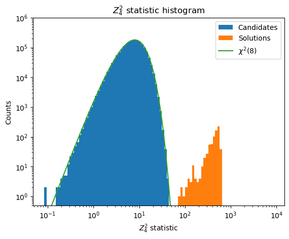
Figure 2: The $Z_{4}^{2}$-test statistic histogram for candidates and solutions generated using the lattice sieving. Here, solutions are significant candidates with a p-value smaller than $10^{-7}$. The $\chi^{2}(8)$ is shown to demonstrate the candidates follow it.

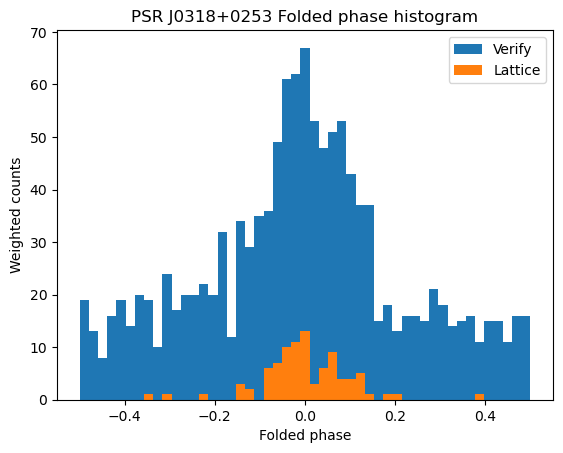
Figure 3: A weighted histogram of one of the solution’s phase fold for the lattice-set and verify-set photons.

8 The norm problem - adapting to bad photons and double pulse profiles

The most severe conceptual problem in our setup is the fact that we are using the $L_{2}$ norm to decide between the different possible solutions.

The $L_{2}$ norm corresponds to the assumption of a perfect Gaussian pulse profile, which doesn’t hold for a vast majority of known $\gamma$-ray pulsars that tend to have a double pulse profile. This is also a bad norm to use when background photons are present, the typical case for sources in Fermi-LAT.

A better choice of a test statistic to rank the different lattice vectors is the H-test Bickel et al. (2008). The H-test corrects for both a somewhat more general pulse shape and for the fact that different TOAs have different association probabilities with the source (at least in the Fermi-LAT case).

Moreover, it is useful to output many vectors out of the lattice sieve and rank them according to the more sensitive H-Test, thereby picking up the correct solution even if the $L_{2}$ norm ranks the correct solution only in the $M$’th place. Sieving algorithms are usually using a large number of vectors, and this approach is beneficial to increase the sensitivity of the search.

Last, the requirement for a large number ($>60$) of photons with high association probability ($p>0.85$) limits the applicability of the method to a few dozen sources (out of the thousands of unassociated sources). In a follow-up paper (Gazith et al. in prep), we will present a novel algorithmic solution that will recover the correct solution in the situation where the association probability of the photons is moderate $\approx 0.5$.

9 Conclusions

In this paper, we have shown that recovering the timing of a pulsar could be done using lattice algorithms, a set of advanced tools developed for cryptanalysis. We have demonstrated that a lattice-based approach can be used to solve a timing model that is a linear combination of known vectors. We showed that lattice algorithms can solve problems that were previously impossible to solve, in a matter of seconds.

We discussed the computational complexity of the technique, which is substantially smaller than full enumeration, and is a strong function of the duty cycle (or the equivalent width, for more complex pulse shapes) and association probabilities.

As a proof of concept, we then solved a real pulsar using Fermi-LAT data. In the next papers in this series, we will show how to linearize a Keplerian orbit and present a novel algorithm that is more computationally efficient, allowing us to solve lattice problems in which half of the TOAs are random or cases where the pulsar has a double pulse profile. We will then apply our methods to all relevant Fermi-LAT unassociated sources.

Appendix A Lattice volume calculation

According to the Gaussian heuristic, the expected length of the shortest vector in a lattice is (per coordinate)

$$\lambda_{1}=\frac{\text{vol}(\mathcal{L})^{1/n}}{\sqrt{2\pi e}}\,,$$ (A1)

where $n$ is the lattice dimension and $\text{vol}(\mathcal{L})$ is the lattice volume, calculated as

$$\text{vol}(\mathcal{L})=\sqrt{\det LL^{T}}\,.$$ (A2)

In our setup, we are interested in the sub-lattice consisting of the unit vectors of the different TOAs, projected orthogonally to the quasi-continuous timing model vectors, the phase residuals lattice. Using the following lattice

$$L=\begin{pmatrix}I_{n\times n}&\mathbb{0}_{n\times m}\\ V_{m\times n}&{\eta}_{m\times m}\\ \end{pmatrix}\,,$$ (A3)

we can write the projection operator that projects out the $\begin{pmatrix}V_{i}&\eta_{i}\end{pmatrix}$ directions, assuming they are normalized appropriately

$$P_{V}=\begin{pmatrix}I_{n\times n}-V^{T}V&-V^{T}\eta\\ -\eta^{T}V&I_{k\times k}-\eta^{T}\eta\\ \end{pmatrix}$$ (A4)

The projected sub-lattice can now be written as

$$\Pi_{n\times n+k}=I_{n\times n+k}P_{V}\,,$$ (A5)

and the matrix we need to calculate its determinant is

$$\Pi\Pi^{T} =I_{n\times n+k}P_{V}P_{V}I_{n+k\times n}$$

$$=I_{n\times n+k}P_{V}I_{n+k\times n}$$

$$=I_{n\times n}-V^{T}V\,.$$ (A6)

Now, to calculate the determinant, we can use the Weinstein–Aronszajn identity

$$\det\Pi\Pi^{T} =\det I_{n\times n}-V^{T}V$$

$$=\det I_{k\times k}-VV^{T}$$

$$=\det I_{k\times k}-(I_{k\times k}-\eta_{k\times k}^{2})$$

$$=\prod_{i}\eta_{i}^{2}\,.$$ (A7)

So the volume of our projected sub-lattice of interest is $\prod_{i}\eta_{i}$,

$$\text{vol}(\mathcal{L})=\prod_{i}\eta_{i}\,.$$ (A8)

References

- Albrecht et al. (2019) Albrecht, M. R., Ducas, L., Herold, G., et al. 2019, The General Sieve Kernel and New Records in Lattice Reduction, Cryptology ePrint Archive, Paper 2019/089. https://eprint.iacr.org/2019/089
- Allen et al. (2013) Allen, B., Knispel, B., Cordes, J. M., et al. 2013, ApJ, 773, 91, doi: 10.1088/0004-637X/773/2/91
- Antoniadis et al. (2022) Antoniadis, J., Arzoumanian, Z., Babak, S., et al. 2022, Monthly Notices of the Royal Astronomical Society, 510, 4873
- Bailes (2022) Bailes, M. 2022, Science, 378, abj3043, doi: 10.1126/science.abj3043
- Ballet et al. (2023) Ballet, J., Bruel, P., Burnett, T., Lott, B., et al. 2023, arXiv preprint arXiv:2307.12546
- Becker et al. (2015) Becker, A., Gama, N., & Joux, A. 2015, Speeding-up lattice sieving without increasing the memory, using sub-quadratic nearest neighbor search, Cryptology ePrint Archive, Paper 2015/522. https://eprint.iacr.org/2015/522
- Bhardwaj et al. (2023) Bhardwaj, M., Michilli, D., Kirichenko, A. Y., et al. 2023, arXiv e-prints, arXiv:2310.10018, doi: 10.48550/arXiv.2310.10018
- Bickel et al. (2008) Bickel, P., Kleijn, B., & Rice, J. 2008, ApJ, 685, 384, doi: 10.1086/590399
- Bruzewski et al. (2023) Bruzewski, S., Schinzel, F. K., & Taylor, G. B. 2023, ApJ, 943, 51, doi: 10.3847/1538-4357/acaa33
- Clark et al. (2023) Clark, C. J., Breton, R. P., Barr, E. D., et al. 2023, MNRAS, 519, 5590, doi: 10.1093/mnras/stac3742
- Cordes & Chatterjee (2019a) Cordes, J. M., & Chatterjee, S. 2019a, ARA&A, 57, 417, doi: 10.1146/annurev-astro-091918-104501
- Cordes & Chatterjee (2019b) —. 2019b, ARA&A, 57, 417, doi: 10.1146/annurev-astro-091918-104501
- development team (2023) development team, T. F. 2023. https://github.com/fplll/fpylll
- Du et al. (2023) Du, C., Huang, Y.-F., Zhang, Z.-B., et al. 2023, arXiv e-prints, arXiv:2310.08971, doi: 10.48550/arXiv.2310.08971
- Ducas (2017) Ducas, L. 2017, Shortest Vector from Lattice Sieving: a Few Dimensions for Free, Cryptology ePrint Archive, Paper 2017/999. https://eprint.iacr.org/2017/999
- Fermi Science Support Development Team (2019) Fermi Science Support Development Team. 2019, Fermitools: Fermi Science Tools, Astrophysics Source Code Library, record ascl:1905.011. http://ascl.net/1905.011
- Fonseca et al. (2020) Fonseca, E., Andersen, B. C., Bhardwaj, M., et al. 2020, ApJ, 891, L6, doi: 10.3847/2041-8213/ab7208
- Frail et al. (2018) Frail, D. A., Ray, P. S., Mooley, K. P., et al. 2018, MNRAS, 475, 942, doi: 10.1093/mnras/stx3281
- Gama et al. (2010) Gama, N., Nguyen, P. Q., & Regev, O. 2010, in Proceedings of the 29th International Conference on Cryptology - EUROCRYPT 2010, Nice, France, 257 – 278, doi: 10.1007/978-3-642-13190-5_13
- Khot (2004) Khot, S. 2004, in 45th Annual IEEE Symposium on Foundations of Computer Science, 126–135, doi: 10.1109/FOCS.2004.31
- Kirsten et al. (2022) Kirsten, F., Marcote, B., Nimmo, K., et al. 2022, Nature, 602, 585, doi: 10.1038/s41586-021-04354-w
- Lenstra et al. (1982) Lenstra, A. K., Lenstra, H. W., & Lovász, L. 1982, Mathematische annalen, 261, 515
- Li et al. (2021) Li, D., Wang, P., Zhu, W. W., et al. 2021, Nature, 598, 267, doi: 10.1038/s41586-021-03878-5
- Lorimer (2008) Lorimer, D. R. 2008, Living reviews in relativity, 11, 1
- Lorimer & Kramer (2004) Lorimer, D. R., & Kramer, M. 2004, Handbook of Pulsar Astronomy, Vol. 4
- Luo et al. (2019) Luo, J., Ransom, S., Demorest, P., et al. 2019, PINT: High-precision pulsar timing analysis package, Astrophysics Source Code Library, record ascl:1902.007. http://ascl.net/1902.007
- Luo et al. (2021) —. 2021, ApJ, 911, 45, doi: 10.3847/1538-4357/abe62f
- Macquart et al. (2020) Macquart, J. P., Prochaska, J. X., McQuinn, M., et al. 2020, Nature, 581, 391, doi: 10.1038/s41586-020-2300-2
- Majid et al. (2021) Majid, W. A., Pearlman, A. B., Prince, T. A., et al. 2021, ApJ, 919, L6, doi: 10.3847/2041-8213/ac1921
- McLaughlin et al. (2009) McLaughlin, M., Lyne, A., Keane, E., et al. 2009, Monthly Notices of the Royal Astronomical Society, 400, 1431
- Mickaliger et al. (2012) Mickaliger, M. B., McLaughlin, M. A., Lorimer, D. R., et al. 2012, ApJ, 760, 64, doi: 10.1088/0004-637X/760/1/64
- Nguyen & Vidick (2008) Nguyen, P. Q., & Vidick, T. 2008, J. of Mathematical Cryptology, 2
- Nieder et al. (2020a) Nieder, L., Allen, B., Clark, C. J., & Pletsch, H. J. 2020a, ApJ, 901, 156, doi: 10.3847/1538-4357/abaf53
- Nieder et al. (2020b) Nieder, L., Clark, C. J., Kandel, D., et al. 2020b, ApJ, 902, L46, doi: 10.3847/2041-8213/abbc02
- Nieder et al. (2020c) —. 2020c, ApJ, 902, L46, doi: 10.3847/2041-8213/abbc02
- Nimmo et al. (2022a) Nimmo, K., Hessels, J. W. T., Kirsten, F., et al. 2022a, Nature Astronomy, 6, 393, doi: 10.1038/s41550-021-01569-9
- Nimmo et al. (2022b) —. 2022b, Nature Astronomy, 6, 393, doi: 10.1038/s41550-021-01569-9
- Niu et al. (2022) Niu, J.-R., Zhu, W.-W., Zhang, B., et al. 2022, Research in Astronomy and Astrophysics, 22, 124004, doi: 10.1088/1674-4527/ac995d
- Pearlman et al. (2018) Pearlman, A. B., Majid, W. A., Prince, T. A., Kocz, J., & Horiuchi, S. 2018, ApJ, 866, 160, doi: 10.3847/1538-4357/aade4d
- Pearlman et al. (2023) Pearlman, A. B., Scholz, P., Bethapudi, S., et al. 2023, arXiv e-prints, arXiv:2308.10930. https://arxiv.org/abs/arXiv:2308.10930
- Petroff et al. (2019) Petroff, E., Hessels, J. W. T., & Lorimer, D. R. 2019, A&A Rev., 27, 4, doi: 10.1007/s00159-019-0116-6
- Phillips & Ransom (2022) Phillips, C., & Ransom, S. 2022, AJ, 163, 84, doi: 10.3847/1538-3881/ac403e
- Platts et al. (2019) Platts, E., Weltman, A., Walters, A., et al. 2019, Phys. Rep., 821, 1, doi: 10.1016/j.physrep.2019.06.003
- Pletsch & Clark (2014) Pletsch, H. J., & Clark, C. J. 2014, ApJ, 795, 75, doi: 10.1088/0004-637X/795/1/75
- Prager et al. (2017) Prager, B. J., Ransom, S. M., Freire, P. C. C., et al. 2017, ApJ, 845, 148, doi: 10.3847/1538-4357/aa7ed7
- Schnorr & Euchner (1994) Schnorr, C., & Euchner, M. 1994, Mathematical Programming, doi: 10.1007/BF01581144
- Snelders et al. (2023) Snelders, M. P., Nimmo, K., Hessels, J. W. T., et al. 2023, Nature Astronomy, 7, 1486, doi: 10.1038/s41550-023-02101-x
- Stairs (2003) Stairs, I. H. 2003, Living Reviews in Relativity, 6, 5, doi: 10.12942/lrr-2003-5
- The CHIME/FRB Collaboration et al. (2019) The CHIME/FRB Collaboration, Andersen, B. C., Bandura, K., et al. 2019, ApJ, 885, L24, doi: 10.3847/2041-8213/ab4a80
- The CHIME/FRB Collaboration et al. (2020) The CHIME/FRB Collaboration, Amiri, M., Andersen, B. C., et al. 2020, Nature, 582, 351, doi: 10.1038/s41586-020-2398-2
- The CHIME/FRB Collaboration et al. (2022) The CHIME/FRB Collaboration, Andersen, B. C., Bandura, K., et al. 2022, Nature, 607, 256, doi: 10.1038/s41586-022-04841-8
- The CHIME/FRB Collaboration et al. (2023) —. 2023, ApJ, 947, 83, doi: 10.3847/1538-4357/acc6c1
- Walters et al. (2018) Walters, A., Weltman, A., Gaensler, B. M., Ma, Y.-Z., & Witzemann, A. 2018, ApJ, 856, 65, doi: 10.3847/1538-4357/aaaf6b
- Xu et al. (2022) Xu, H., Niu, J. R., Chen, P., et al. 2022, Nature, 609, 685, doi: 10.1038/s41586-022-05071-8