Towards Fast Stochastic Sampling in Diffusion Generative Models

Abstract

Diffusion models suffer from slow sample generation at inference time. Despite recent efforts, improving the sampling efficiency of stochastic samplers for diffusion models remains a promising direction. We propose Splitting Integrators for fast stochastic sampling in pre-trained diffusion models in augmented spaces. Commonly used in molecular dynamics, splitting-based integrators attempt to improve sampling efficiency by cleverly alternating between numerical updates involving the data, auxiliary, or noise variables. However, we show that a naive application of splitting integrators is sub-optimal for fast sampling. Consequently, we propose several principled modifications to naive splitting samplers for improving sampling efficiency and denote the resulting samplers as Reduced Splitting Integrators. In the context of Phase Space Langevin Diffusion (PSLD)Pandey & Mandt, 2023 on CIFAR-10, our stochastic sampler achieves an FID score of 2.36 in only 100 network function evaluations (NFE) as compared to 2.63 for the best baselines.

1 Introduction

Diffusion models [1, 2, 3, 4] have demonstrated impressive performance on various tasks, such as image and video synthesis [5, 6, 7, 8, 9, 10, 11, 12], image super-resolution [13], and audio and speech synthesis [14, 15]. However, we identify two problems with the current landscape for fast sampling in diffusion models.

Firstly, while fast sample generation in diffusion models is an active area of research, recent advances have mostly focused on accelerating deterministic samplers [16, 17, 18]. However, the latter does not achieve optimal sample quality even with a large NFE budget and may require specialized training improvements [19]. In contrast, stochastic samplers usually achieve better sample quality but require a larger sampling budget than their deterministic counterparts.

Secondly, most efforts to improve diffusion model sampling have focused on a specific family of models that perform diffusion in the data space [4, 19]. However, recent work [20, 21, 22] indicates that performing diffusion in a joint space, where the data space is augmented with auxiliary variables, can improve sample quality and likelihood over data-space-only diffusion models. However, improving the sampling efficiency for augmented diffusion models is still underexplored but a promising avenue for further improvements. Therefore, a generic framework is required for faster sampling from a broader class of diffusion models.

Problem Statement: Efficient Stochastic Sampling during Inference. Our goal is to develop efficient stochastic samplers that are applicable to sampling from a broader class of diffusion models (for instance, augmented diffusion models like PSLD [21]) and achieve high-fidelity samples, even when the NFE budget is greatly reduced, e.g., from 1000 to 100 or even 50. We evaluate the effectiveness of the proposed samplers in the context of PSLD [21] due to its strong empirical performance. However, the presented techniques are also applicable to other diffusion models.

Contributions. Taking inspiration from molecular dynamics [23], we present Splitting Integrators for efficient sampling in diffusion models. However, we show that their naive application can be sub-optimal for sampling efficiency. Therefore, based on local error analysis for numerical solvers [24], we present several improvements to our naive schemes to achieve improved sample efficiency. We denote the resulting samplers as Reduced Splitting Integrators.

2 Background

We provide relevant background on diffusion models and their augmented versions. Specifically, diffusion models assume that a continuous-time forward process (with affine drift),

$$d{\mathbf{z}}_{t}={\bm{F}}_{t}{\mathbf{z}}_{t}\,dt+{\bm{G}}_{t}\,d{\mathbf{w}}_{t},\quad t\in[0,T],$$ (1)

with a standard Wiener process ${\mathbf{w}}_{t}$, time-dependent matrix ${\bm{F}}\colon[0,T]\to\mathbb{R}^{d\times d}$, and diffusion coefficient ${\bm{G}}\colon[0,T]\to\mathbb{R}^{d\times d}$, converts data ${\mathbf{z}}_{0}\in\mathbb{R}^{d}$ into noise. A reverse SDE specifies how data is generated from noise [4, 25],

$$d{\mathbf{z}}_{t}=\left[{\bm{F}}_{t}{\mathbf{z}}_{t}-{\bm{G}}_{t}{\bm{G}}_{t}^{\top}\nabla_{{\mathbf{x}}_{t}}\log p_{t}({\mathbf{z}}_{t})\right]\,dt+{\bm{G}}_{t}d\bar{\mathbf{w}}_{t},$$ (2)

which involves the score ($\nabla_{{\mathbf{z}}_{t}}\log p_{t}({\mathbf{z}}_{t})$) of the marginal distribution over ${\mathbf{z}}_{t}$ at time $t$. The score is intractable to compute and is approximated using a parametric estimator ${\bm{s}}_{\theta}({\mathbf{z}}_{t},t)$, trained using denoising score matching [2, 4, 26]. Once the score has been learned, generating new data samples involves sampling noise from the stationary distribution of Eqn. 1 (typically an isotropic Gaussian) and numerically integrating Eqn. 2, resulting in a stochastic sampler. Next, we highlight two classes of diffusion models.

Non-Augmented Diffusions. Many existing diffusion models are formulated purely in data space, i.e., ${\mathbf{z}}_{t}={\mathbf{x}}_{t}\in\mathbb{R}^{d}$. One popular example is the Variance Preserving (VP)-SDE [4] with ${\bm{F}}_{t}=-\frac{1}{2}\beta_{t}{\bm{I}}_{d},{\bm{G}}_{t}=\sqrt{\beta_{t}}{\bm{I}}_{d}$. Recently, Karras et al. [19] instead propose a re-scaled process, with ${\bm{F}}_{t}=\bm{0}_{d},{\bm{G}}_{t}=\sqrt{2\dot{\sigma}_{t}\sigma_{t}}{\bm{I}}_{d}$ ,which allows for faster sampling during generation. Here $\beta_{t},\sigma_{t}\in\mathbb{R}$ define the noise schedule in their respective diffusion processes.

Augmented Diffusions. For augmented diffusions, the data (or position) space, ${\mathbf{x}}_{t}$, is coupled with auxiliary (a.k.a momentum) variables, ${\mathbf{m}}_{t}$, and diffusion is performed in the joint space. For instance, Pandey and Mandt [21] propose PSLD, where ${\mathbf{z}}_{t}=[{\mathbf{x}}_{t},{\mathbf{m}}_{t}]^{T}\in\mathbb{R}^{2d}$. Moreover,

$${\bm{F}}_{t}=\left(\frac{\beta}{2}\begin{pmatrix}-\Gamma&M^{-1}\\ -1&-\nu\end{pmatrix}\otimes{\bm{I}}_{d}\right),\quad\quad{\bm{G}}_{t}=\left(\begin{pmatrix}\sqrt{\Gamma\beta}&0\\ 0&\sqrt{M\nu\beta}\end{pmatrix}\otimes{\bm{I}}_{d}\right),$$ (3)

where $\{\beta,\Gamma,\nu,M^{-1}\}\in\mathbb{R}$ are the SDE hyperparameters. Augmented diffusions have been shown to exhibit better sample quality with a faster generation process [20, 21], and better likelihood estimation [22] over their non-augmented counterparts. In this work, we focus on sample quality and, therefore, study the efficient samplers we develop in the PSLD setting.

3 Splitting Integrators for Fast Stochastic Sampling

Splitting integrators are commonly used to design symplectic numerical solvers for molecular dynamics systems [23]. However, their application for fast diffusion sampling is still underexplored [20]. The main intuition behind splitting integrators is to split an ODE/SDE into subcomponents, which are then independently solved numerically (or analytically). The resulting updates are then composed in a specific order to obtain the final solution. We briefly introduce splitting integrators in Appendix A.1 and refer interested readers to Leimkuhler [23] for a detailed discussion. Splitting integrators are particularly suited for augmented diffusion models since they can leverage the split into position and momentum variables for faster sampling. However, their application for fast sampling in position-space-only diffusion models [4, 19] remains an interesting direction for future work.

Naive Stochastic Splitting Integrators. We apply splitting integrators to the PSLD Reverse SDE and use the following splitting scheme.

$$\begin{pmatrix}d\bar{{\mathbf{x}}}_{t}\\ d\bar{{\mathbf{m}}}_{t}\end{pmatrix}=\underbrace{\frac{\beta}{2}\begin{pmatrix}2\Gamma\bar{{\mathbf{x}}}_{t}-M^{-1}\bar{{\mathbf{m}}}_{t}+2\Gamma{\bm{s}}_{\theta}^{x}(\bar{{\mathbf{z}}}_{t},t)\\ 0\end{pmatrix}dt}_{A}+O+\underbrace{\frac{\beta}{2}\begin{pmatrix}0\\ \bar{{\mathbf{x}}}_{t}+2\nu\bar{{\mathbf{m}}}_{t}+2M\nu{\bm{s}}_{\theta}^{m}(\bar{{\mathbf{z}}}_{t},t)\end{pmatrix}dt}_{B}.$$

where $\bar{{\mathbf{x}}}_{t}={\mathbf{x}}_{T-t}$, $\bar{{\mathbf{m}}}_{t}={\mathbf{m}}_{T-t}$, ${\bm{s}}_{{\bm{\theta}}}^{x}$ and ${\bm{s}}_{{\bm{\theta}}}^{m}$ denote the score components in the data and momentum space, respectively, and $O=\begin{pmatrix}-\frac{\beta\Gamma}{2}\bar{{\mathbf{x}}}_{t}dt+\sqrt{\beta\Gamma}d\bar{{\mathbf{w}}}_{t}\\ -\frac{\beta\nu}{2}\bar{{\mathbf{m}}}_{t}dt+\sqrt{M\nu\beta}d\bar{{\mathbf{w}}}_{t}\end{pmatrix}$ represents the Ornstein-Uhlenbeck process in the joint space. Given step size $h$, we further denote the Euler updates for the components $A$, $B$ and $O$ as $\mathcal{L}_{h}^{A}$, $\mathcal{L}_{h}^{B}$ and $\mathcal{L}_{h}^{O}$, respectively. These updates can be composed differently to yield a valid stochastic sampler. Among several possible composition schemes, we find OBA, BAO, and OBAB to work particularly well (See Appendix A.2 for complete numerical updates). We refer to these schemes as Naive Splitting Integrators. Consequently, we denote these samplers as NOBA, NBAO, and NOBAB, respectively. For an empirical evaluation, we utilize a PSLD model [21] ($\Gamma=0.01,\nu=4.01$) pre-trained on CIFAR-10. We measure sampling efficiency via network function evaluations (NFE) and measure sample quality using FID [27]. Our proposed naive samplers outperform the baseline Euler-Maruyama (EM) sampler (Fig. 1(a)). This is intuitive since, unlike EM, the proposed naive samplers alternate between updates in the momentum and the position space, thus exploiting the coupling between the data and the momentum variables. Next, we propose several modifications to the naive schemes to further improve sampling efficiency.

(a)

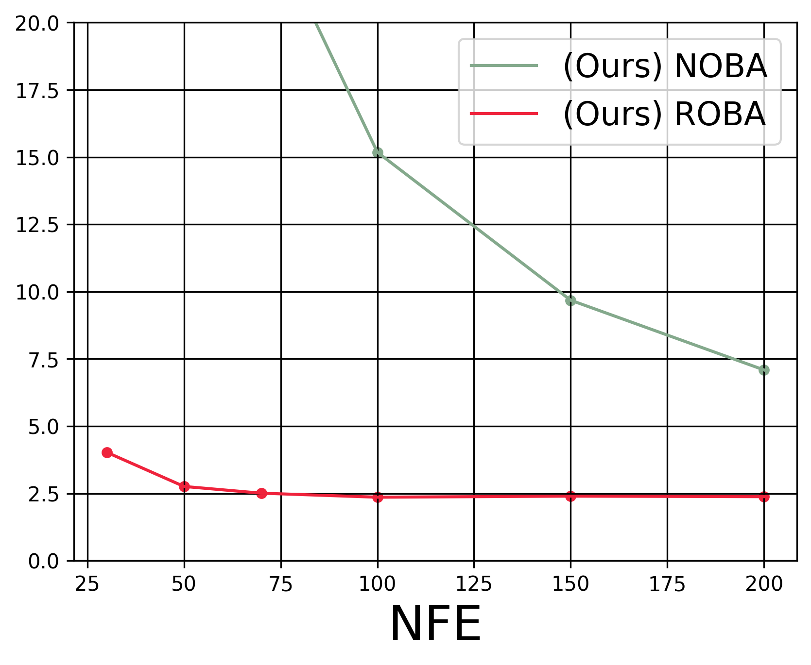
(b)

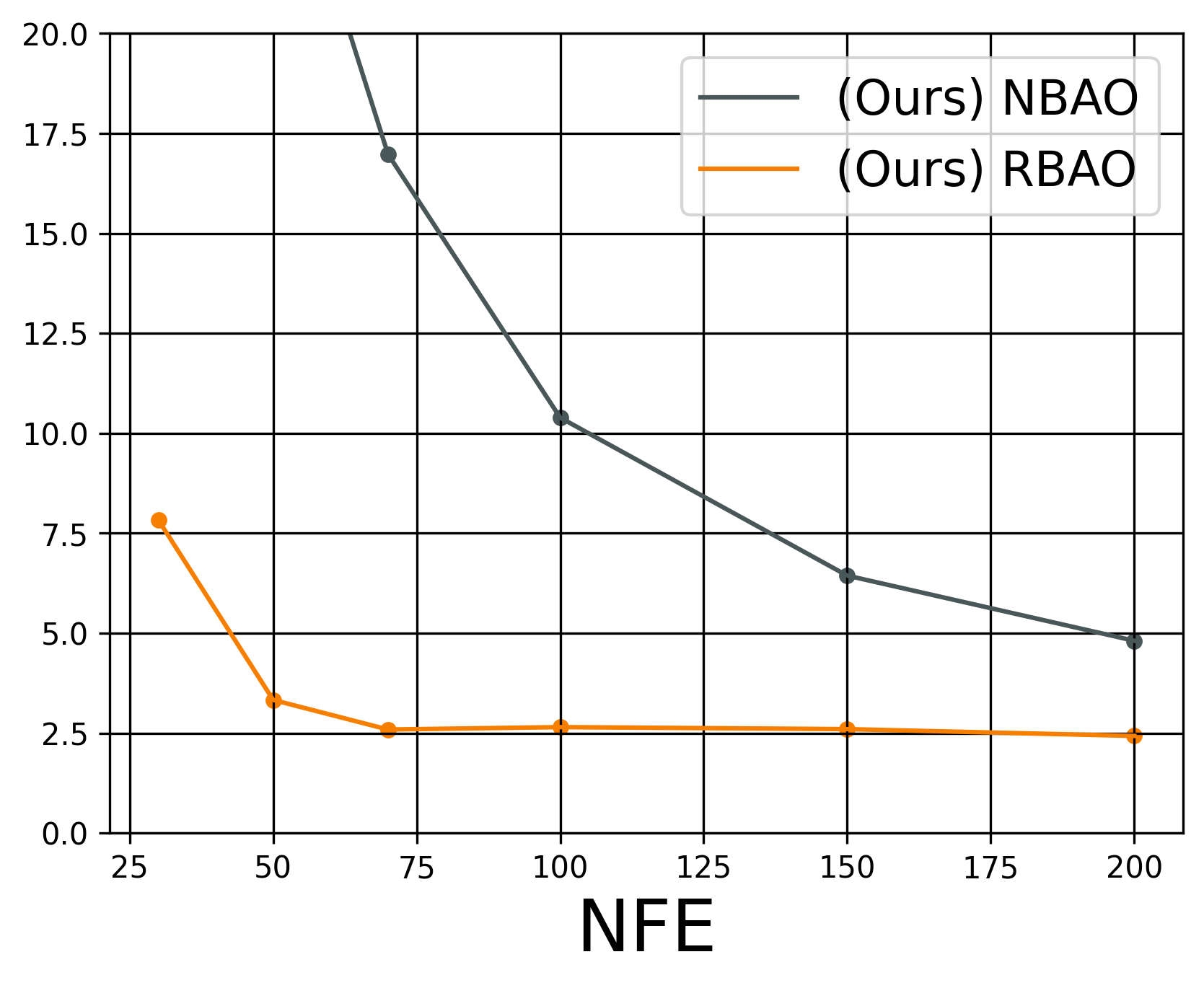
(c)

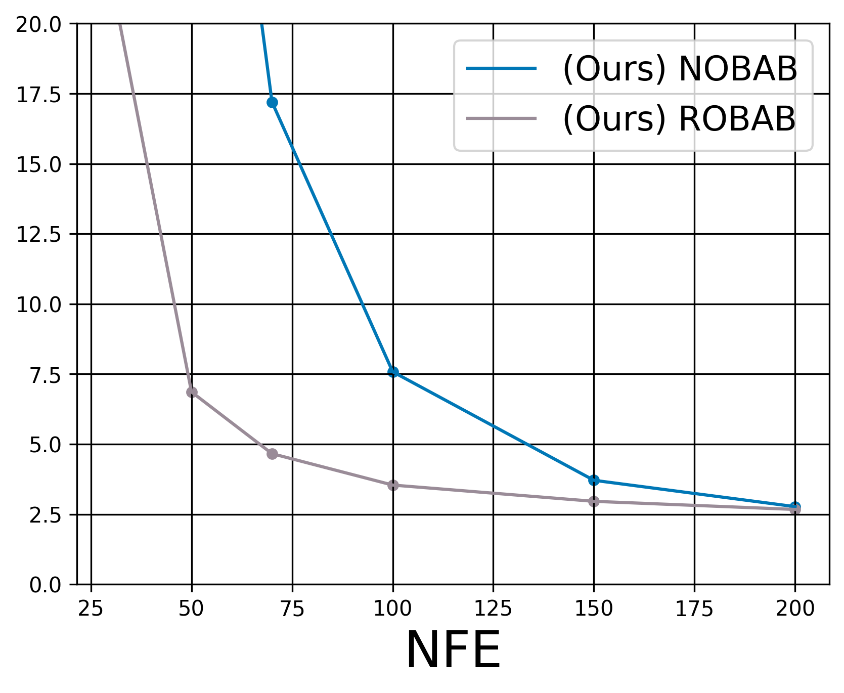
(d)

Figure 1: Splitting integrators for fast stochastic sampling in diffusion models. a) Sample quality comparisons between naive splitting schemes and the EM Sampler. (b-d) Reduced Splitting schemes outperform their naive counterparts by a large margin. (Left to Right) Comparisons between the naive splitting schemes and their reduced counterparts for the OBA, BAO, and OBAB samplers.

Reduced Stochastic Splitting Integrators. While the proposed naive schemes perform well, Fig. 1(a) also suggests scope for improvement, especially at low NFE budgets. This suggests the need for a deeper insight into the error analysis for the naive schemes. Therefore, based on local error analysis for SDEs, we propose the following modifications to our naive samplers.

• Firstly, we reuse the score function evaluation between the first consecutive position and the momentum updates.

• Secondly, for sampling schemes involving half-steps (i.e. with step-size $h/2$ like NOBAB), we evaluate the score in the last step with a timestep embedding of $T-(t+h)$ instead of $T-t$.

• Lastly, similar to Karras et al. [19], we introduce a parameter $\lambda_{s}$ in the position space update for $\mathcal{L}_{O}$ to control the amount of noise injected in the position space. However, adding a similar parameter in the momentum space led to unstable behavior. Therefore, we restrict this adjustment to the position space. For a given sampling budget, we explicitly adjust $\lambda_{s}$ for optimal sample quality via a simple grid search during inference. We include more details in Appendix A.2.2

Applying these modifications to naive splitting integrators yields Reduced Splitting Integrators. Consequently, we denote these samplers as ROBA, RBAO, and ROBAB, respectively (See Appendix A.2.3 for complete numerical updates). Figures 1(b)-1(d) compare the performance of our reduced samplers with their naive counterparts. Empirically, our modifications significantly improve sample quality for all three samplers (Fig. 1(b)-1(d)). This is because our proposed modifications serve the following benefits.

• First, re-using the score function evaluation between the first consecutive updates in the data and the momentum space reduces the number of NFE s per update step by one for all reduced samplers, which enables smaller step sizes for the same compute budget during sampling and hence largely reduces numerical discretization errors.

• Secondly, re-using the score function evaluation leads to canceling certain error terms arising from numerical discretization, which is especially helpful for low NFE budgets.

• Lastly, as also noted in recent works [19, 28], the choice of the variance of the noise injected during stochastic sampling can largely affect sample quality.

4 Additional Experimental Results

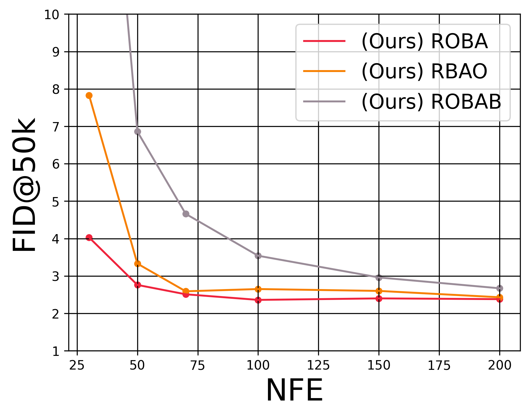
(a)

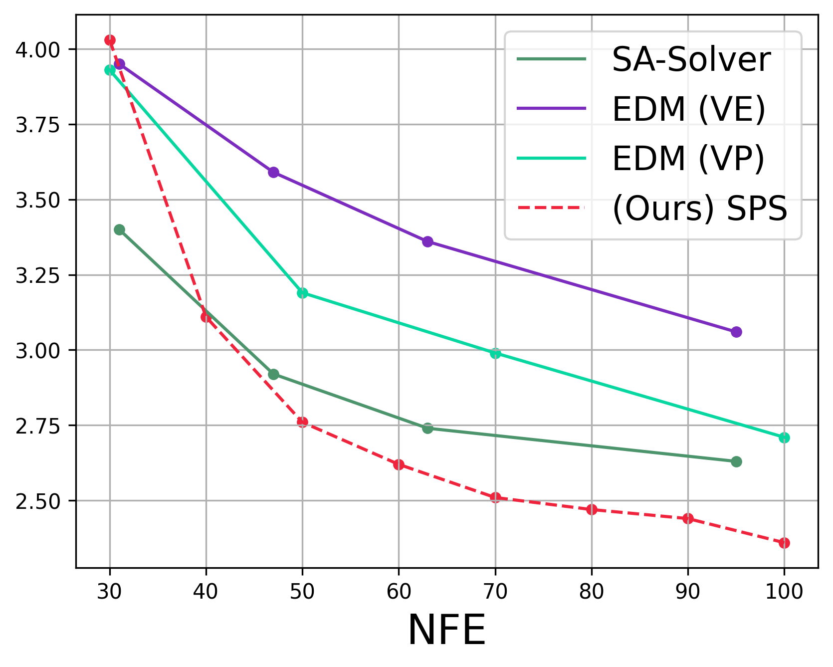
(b)

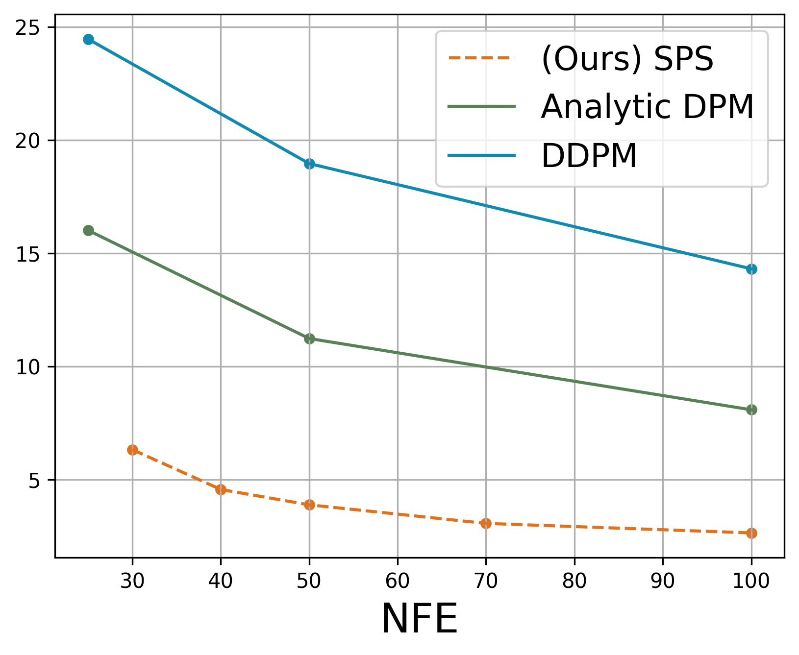
(c)

Figure 2: Comparison with state-of-the-art methods. a) Reduced OBA outperforms other reduced splitting schemes. (b, c) SPS outperforms competing baseline methods for stochastic sampling for the CIFAR-10 and CelebA-64 datasets, respectively.

Datasets and Evaluation Metrics. We use the CIFAR-10 and the CelebA-64 [29] datasets for comparisons. Unless specified otherwise, we report FID for 50k generated samples for all datasets and quantify sampling efficiency using NFE. We use the pre-trained models from PSLD [21] and use a last-step denoising step [30, 4] when sampling from the proposed samplers.

Baselines and setup. While the techniques presented in this work are generally applicable to other types of diffusion models, we compare our best-performing reduced splitting integrator, ROBA (see Fig. 2(a)), with recent work on fast stochastic sampling in diffusion models including SA-Solver [31], SEEDS [32], EDM [19] and Analytic DPM [28]. We also compare with another splitting-based sampler, SSCS [20], applied to the PSLD reverse SDE. We denote our best-performing sampler as Splitting-based PSLD Sampler (SPS) for notational convenience.

Empirical Results. For CIFAR-10, our SDE sampler outperforms all other baselines for different compute budgets (Fig. 2(b)). We make similar observations for the CelebA-64 dataset, where our proposed samplers can obtain significant gains over prior methods (see Fig. 2(c)). More specifically, our SDE sampler achieves an FID score of 2.36 and 2.64 for the CIFAR-10 and CelebA-64 datasets, respectively, in just 100 network function evaluations. We include additional results in Appendix C.

5 Conclusion

We present a splitting integrator for fast stochastic sampling from a broader class of diffusion models. We show that a naive application of splitting integrators can be sub-optimal for sample quality. To this end, we propose a few modifications to our naive samplers and denote the resulting sampler as Reduced Splitting Integrators, which outperform existing baselines for fast stochastic sampling. Empirically, we find that controlling the amount of stochasticity injected in the data space during sampling can largely affect sample quality for the proposed splitting integrators. Therefore, further investigation into the theoretical aspects of optimal noise injection in stochastic sampling can be an interesting direction for future work. We also believe that exploring similar splitting samplers for position-space-only diffusion models like Stable-Diffusion [7] could also be an interesting direction for further work.

Appendix A Splitting Integrators

A.1 Introduction to Splitting Integrators

Here, we provide a brief introduction to splitting integrators. For a detailed account of splitting integrators for designing symplectic numerical methods, we refer interested readers to Leimkuhler [23]. As discussed in the main text, the main idea behind splitting integrators is to split the vector field of an ODE or the drift and the diffusion components of an SDE into independent subcomponents, which are then solved independently using a numerical scheme (or analytically). The solutions to independent sub-components are then composed in a specific order to obtain the final solution. Thus, three key steps in designing a splitting integrator are split, solve, and compose. We illustrate these steps with an example of a deterministic dynamical system. However, the concept is generic and can be applied to systems with stochastic dynamics as well.

Consider a dynamical system specified by the following ODE:

$$\begin{pmatrix}d{\mathbf{x}}_{t}\\ d{\mathbf{m}}_{t}\end{pmatrix}=\begin{pmatrix}{\bm{f}}({\mathbf{x}}_{t},{\mathbf{m}}_{t})\\ {\bm{g}}({\mathbf{x}}_{t},{\mathbf{m}}_{t})\end{pmatrix}dt$$ (4)

We start by choosing a scheme to split the vector field for the ODE in Eqn. 4. While different types of splitting schemes can be possible, we choose the following scheme for this example,

$$\begin{pmatrix}d{\mathbf{x}}_{t}\\ d{\mathbf{m}}_{t}\end{pmatrix}=\underbrace{\begin{pmatrix}{\bm{f}}({\mathbf{x}}_{t},{\mathbf{m}}_{t})\\ 0\end{pmatrix}dt}_{A}+\underbrace{\begin{pmatrix}0\\ {\bm{g}}({\mathbf{x}}_{t},{\mathbf{m}}_{t})\end{pmatrix}dt}_{B}$$ (5)

where we denote the individual components by $A$ and $B$. Next, we solve each of these components independently, i.e., we compute solutions for the following ODEs independently.

$$\begin{pmatrix}d{\mathbf{x}}_{t}\\ d{\mathbf{m}}_{t}\end{pmatrix}=\begin{pmatrix}{\bm{f}}({\mathbf{x}}_{t},{\mathbf{m}}_{t})\\ 0\end{pmatrix}dt,\quad\quad\begin{pmatrix}d{\mathbf{x}}_{t}\\ d{\mathbf{m}}_{t}\end{pmatrix}=\begin{pmatrix}0\\ {\bm{g}}({\mathbf{x}}_{t},{\mathbf{m}}_{t})\end{pmatrix}dt$$ (6)

While any numerical scheme can be used to approximate the solution for the splitting components, we use Euler throughout this work. Therefore, applying an Euler approximation, with a step size $h$, to each of these splitting components yields the solutions $\mathcal{L}^{A}_{h}$ and $\mathcal{L}^{B}_{h}$, as follows,

$$\mathcal{L}^{A}_{h}=\begin{cases}{\mathbf{x}}_{t+h}={\mathbf{x}}_{t}+h{\bm{f}}({\mathbf{x}}_{t},{\mathbf{m}}_{t})\\ {\mathbf{m}}_{t+h}={\mathbf{m}}_{t}\end{cases},\quad\mathcal{L}^{B}_{h}=\begin{cases}{\mathbf{x}}_{t+h}={\mathbf{x}}_{t}\\ {\mathbf{m}}_{t+h}={\mathbf{m}}_{t}+h{\bm{g}}({\mathbf{x}}_{t},{\mathbf{m}}_{t})\end{cases}$$ (7)

In the final step, we compose the solutions to the independent components in a specific order. For instance, for the composition scheme AB, the final solution $\mathcal{L}^{[AB]}_{h}=\mathcal{L}^{B}_{h}\circ\mathcal{L}^{A}_{h}$. Therefore,

$$\mathcal{L}^{[AB]}_{h}=\begin{cases}{\mathbf{x}}_{t+h}={\mathbf{x}}_{t}+h{\bm{f}}({\mathbf{x}}_{t},{\mathbf{m}}_{t})\\ {\mathbf{m}}_{t+h}={\mathbf{m}}_{t}+h{\bm{g}}({\mathbf{x}}_{t+h},{\mathbf{m}}_{t})\end{cases}$$ (8)

is the required solution. It is worth noting that the final solution depends on the chosen composition scheme, and often it is not clear beforehand which composition scheme might work best.

A.2 Stochastic Splitting Integrators

We split the Reverse Diffusion SDE for PSLD using the following splitting scheme.

$$\begin{pmatrix}d\bar{{\mathbf{x}}}_{t}\\ d\bar{{\mathbf{m}}}_{t}\end{pmatrix}=\underbrace{\frac{\beta}{2}\begin{pmatrix}2\Gamma\bar{{\mathbf{x}}}_{t}-M^{-1}\bar{{\mathbf{m}}}_{t}+2\Gamma{\bm{s}}_{\theta}^{x}(\bar{{\mathbf{z}}}_{t},t)\\ 0\end{pmatrix}dt}_{A}+O+\underbrace{\frac{\beta}{2}\begin{pmatrix}0\\ \bar{{\mathbf{x}}}_{t}+2\nu\bar{{\mathbf{m}}}_{t}+2M\nu{\bm{s}}_{\theta}^{m}(\bar{{\mathbf{z}}}_{t},t)\end{pmatrix}dt}_{B}$$ (9)

where $O=\begin{pmatrix}-\frac{\beta\Gamma}{2}\bar{{\mathbf{x}}}_{t}dt+\sqrt{\beta\Gamma}d\bar{{\mathbf{w}}}_{t}\\ -\frac{\beta\nu}{2}\bar{{\mathbf{m}}}_{t}dt+\sqrt{M\nu\beta}d\bar{{\mathbf{w}}}_{t}\end{pmatrix}$ is the Ornstein-Uhlenbeck component which injects stochasticity during sampling. Similar to the deterministic case, $\bar{{\mathbf{x}}}_{t}={\mathbf{x}}_{T-t}$, $\bar{{\mathbf{m}}}_{t}={\mathbf{m}}_{T-t}$, ${\bm{s}}_{{\bm{\theta}}}^{x}$ and ${\bm{s}}_{{\bm{\theta}}}^{m}$ denote the score components in the data and momentum space, respectively. We approximate the solution for splits $A$ and $B$ using a simple Euler-based numerical approximation. Formally, we denote the Euler approximation for the splits $A$ and $B$ by $\mathcal{L}_{A}$ and $\mathcal{L}_{B}$, respectively, with their corresponding numerical updates specified as:

$$\mathcal{L}_{A} :\begin{cases}\bar{{\mathbf{x}}}_{t+h}&=\bar{{\mathbf{x}}}_{t}+\frac{h\beta}{2}\Big{[}2\Gamma\bar{{\mathbf{x}}}_{t}-M^{-1}\bar{{\mathbf{m}}}_{t}+2\Gamma{\bm{s}}_{\theta}^{x}(\bar{{\mathbf{x}}}_{t},\bar{{\mathbf{m}}}_{t},T-t)\Big{]}\\ \bar{{\mathbf{m}}}_{t+h}&=\bar{{\mathbf{m}}}_{t}\end{cases}$$ (10)

$$\mathcal{L}_{B} :\begin{cases}\bar{{\mathbf{x}}}_{t+h}&=\bar{{\mathbf{x}}}_{t}\\ \bar{{\mathbf{m}}}_{t+h}&=\bar{{\mathbf{m}}}_{t}+\frac{h\beta}{2}\Big{[}\bar{{\mathbf{x}}}_{t}+2\nu\bar{{\mathbf{m}}}_{t}+2M\nu{\bm{s}}_{\theta}^{m}(\bar{{\mathbf{x}}}_{t},\bar{{\mathbf{m}}}_{t},T-t)\Big{]}\end{cases}$$ (11)

It is worth noting that the solution to the OU component can be computed analytically:

$$\mathcal{L}_{O}:\begin{cases}\bar{{\mathbf{x}}}_{t+h}&=\exp{\left(\frac{-h\beta\Gamma}{2}\right)}\bar{{\mathbf{x}}}_{t}+\sqrt{1-\exp{\left(-h\beta\Gamma\right)}}\bm{\epsilon}_{x},\;\;\;\;\bm{\epsilon}_{x}\sim\mathcal{N}(\bm{0}_{d},{\bm{I}}_{d})\\ \bar{{\mathbf{m}}}_{t+h}&=\exp{\left(\frac{-h\beta\nu}{2}\right)}\bar{{\mathbf{m}}}_{t}+\sqrt{M}\sqrt{1-\exp{\left(-h\beta\nu\right)}}\bm{\epsilon}_{m},\;\;\;\;\bm{\epsilon}_{m}\sim\mathcal{N}(\bm{0}_{d},{\bm{I}}_{d})\end{cases}$$ (12)

Next, we highlight the numerical update equations for the Naive OBA, BAO, and OBAB samplers and their corresponding reduced analogues.

A.2.1 Naive Splitting Samplers

Naive OBA: In this scheme, for a given step size h, the solutions to the splitting pieces $\mathcal{L}_{h}^{A}$, $\mathcal{L}_{h}^{B}$ and $\mathcal{L}_{h}^{O}$ are composed as $\mathcal{L}^{[OBA]}_{h}=\mathcal{L}^{A}_{h}\circ\mathcal{L}^{B}_{h}\circ\mathcal{L}^{O}_{h}$. Consequently, one numerical update step for this integrator can be defined as,

$$\bar{{\mathbf{x}}}_{t+h} =\exp{\left(\frac{-h\beta\Gamma}{2}\right)}\bar{{\mathbf{x}}}_{t}+\sqrt{1-\exp{\left(-h\beta\Gamma\right)}}\bm{\epsilon}_{x}$$ (13)

$$\bar{{\mathbf{m}}}_{t+h} =\exp{\left(\frac{-h\beta\nu}{2}\right)}\bar{{\mathbf{m}}}_{t}+\sqrt{M}\sqrt{1-\exp{\left(-h\beta\nu\right)}}\bm{\epsilon}_{m}$$ (14)

$$\hat{{\mathbf{m}}}_{t+h} =\bar{{\mathbf{m}}}_{t+h}+\frac{h\beta}{2}\left[\bar{{\mathbf{x}}}_{t+h}+2\nu\bar{{\mathbf{m}}}_{t+h}+2M\nu{\bm{s}}_{\theta}^{m}(\bar{{\mathbf{x}}}_{t+h},\bar{{\mathbf{m}}}_{t+h},T-t)\right]$$ (15)

$$\hat{{\mathbf{x}}}_{t+h} =\bar{{\mathbf{x}}}_{t+h}+\frac{h\beta}{2}\left[2\Gamma\bar{{\mathbf{x}}}_{t+h}-M^{-1}\hat{{\mathbf{m}}}_{t+h}+2\Gamma{\bm{s}}_{\theta}^{x}(\bar{{\mathbf{x}}}_{t+h},\hat{{\mathbf{m}}}_{t+h},T-t)\right]$$ (16)

where $\bm{\epsilon}_{x},\bm{\epsilon}_{m}\sim\mathcal{N}(\bm{0}_{d},{\bm{I}}_{d})$. Therefore, one update step for Naive OBA requires two NFEs.

Naive BAO: Given a step size h, the solutions to the splitting pieces $\mathcal{L}_{h}^{A}$, $\mathcal{L}_{h}^{B}$ and $\mathcal{L}_{h}^{O}$ are composed as $\mathcal{L}^{[BAO]}_{h}=\mathcal{L}^{O}_{h}\circ\mathcal{L}^{A}_{h}\circ\mathcal{L}^{B}_{h}$. Consequently, one numerical update step for this integrator can be defined as,

$$\bar{{\mathbf{m}}}_{t+h} =\bar{{\mathbf{m}}}_{t}+\frac{h\beta}{2}\left[\bar{{\mathbf{x}}}_{t}+2\nu\bar{{\mathbf{m}}}_{t}+2M\nu{\bm{s}}_{\theta}^{m}(\bar{{\mathbf{x}}}_{t},\bar{{\mathbf{m}}}_{t},T-t)\right]$$ (17)

$$\bar{{\mathbf{x}}}_{t+h} =\bar{{\mathbf{x}}}_{t}+\frac{h\beta}{2}\left[2\Gamma\bar{{\mathbf{x}}}_{t}-M^{-1}\bar{{\mathbf{m}}}_{t+h}+2\Gamma{\bm{s}}_{\theta}^{x}(\bar{{\mathbf{x}}}_{t},\bar{{\mathbf{m}}}_{t+h},T-t)\right]$$ (18)

$$\hat{{\mathbf{x}}}_{t+h} =\exp{\left(\frac{-h\beta\Gamma}{2}\right)}\bar{{\mathbf{x}}}_{t+h}+\sqrt{1-\exp{\left(-h\beta\Gamma\right)}}\bm{\epsilon}_{x}$$ (19)

$$\hat{{\mathbf{m}}}_{t+h} =\exp{\left(\frac{-h\beta\nu}{2}\right)}\bar{{\mathbf{m}}}_{t+h}+\sqrt{M}\sqrt{1-\exp{\left(-h\beta\nu\right)}}\bm{\epsilon}_{m}$$ (20)

where $\bm{\epsilon}_{x},\bm{\epsilon}_{m}\sim\mathcal{N}(\bm{0}_{d},{\bm{I}}_{d})$. Therefore, one update step for Naive BAO requires two NFEs.

Naive OBAB: Given a step size h, the solutions to the splitting pieces $\mathcal{L}_{h}^{A}$, $\mathcal{L}_{h}^{B}$ and $\mathcal{L}_{h}^{O}$ are composed as $\mathcal{L}^{[OBAB]}_{h}=\mathcal{L}^{B}_{h/2}\circ\mathcal{L}^{A}_{h}\circ\mathcal{L}^{B}_{h/2}\circ\mathcal{L}^{O}_{h}$. Consequently, one numerical update step for this integrator can be defined as,

$$\bar{{\mathbf{x}}}_{t+h} =\exp{\left(\frac{-h\beta\Gamma}{2}\right)}\bar{{\mathbf{x}}}_{t}+\sqrt{1-\exp{\left(-h\beta\Gamma\right)}}\bm{\epsilon}_{x}$$ (21)

$$\bar{{\mathbf{m}}}_{t+h} =\exp{\left(\frac{-h\beta\nu}{2}\right)}\bar{{\mathbf{m}}}_{t}+\sqrt{M}\sqrt{1-\exp{\left(-h\beta\nu\right)}}\bm{\epsilon}_{m}$$ (22)

$$\hat{{\mathbf{m}}}_{t+h/2} =\bar{{\mathbf{m}}}_{t+h}+\frac{h\beta}{4}\left[\bar{{\mathbf{x}}}_{t+h}+2\nu\bar{{\mathbf{m}}}_{t+h}+2M\nu{\bm{s}}_{\theta}^{m}(\bar{{\mathbf{x}}}_{t+h},\bar{{\mathbf{m}}}_{t+h},T-t)\right]$$ (23)

$$\hat{{\mathbf{x}}}_{t+h} =\bar{{\mathbf{x}}}_{t+h}+\frac{h\beta}{2}\left[2\Gamma\bar{{\mathbf{x}}}_{t+h}-M^{-1}\hat{{\mathbf{m}}}_{t+h/2}+2\Gamma{\bm{s}}_{\theta}^{x}(\bar{{\mathbf{x}}}_{t+h},\hat{{\mathbf{m}}}_{t+h/2},T-t)\right]$$ (24)

$$\hat{{\mathbf{m}}}_{t+h} =\hat{{\mathbf{m}}}_{t+h/2}+\frac{h\beta}{4}\left[\hat{{\mathbf{x}}}_{t+h}+2\nu\hat{{\mathbf{m}}}_{t+h/2}+2M\nu{\bm{s}}_{\theta}^{m}(\hat{{\mathbf{x}}}_{t+h},\hat{{\mathbf{m}}}_{t+h/2},T-t)\right]$$ (25)

where $\bm{\epsilon}_{x},\bm{\epsilon}_{m}\sim\mathcal{N}(\bm{0}_{d},{\bm{I}}_{d})$. Therefore, one update step for Naive OBAB requires three NFEs.

A.2.2 Effects of controlling stochasticity

Similar to Karras et al. [19], we introduce a parameter $\lambda_{s}$ in the position space update for $\mathcal{L}_{O}$ to control the amount of noise injected in the position space. More specifically, we modify the numerical update equations for the Ornstein-Uhlenbeck process in the position space as follows:

$$\bar{{\mathbf{x}}}_{t+h}=\exp{\left(\frac{-h\beta\Gamma}{2}\right)}\bar{{\mathbf{x}}}_{t}+\sqrt{1-\exp{\left(-\bar{t}\lambda_{s}\beta\Gamma\right)}}\bm{\epsilon}_{x},\;\;\;\;\bm{\epsilon}_{x}\sim\mathcal{N}(\bm{0}_{d},{\bm{I}}_{d})$$ (26)

where $\bar{t}=\frac{(T-t)+(T-t-h)}{2}$, i.e., the mid-point for two consecutive time steps during sampling. Our choice of $\bar{t}$ is primarily based on empirical results. Moreover, we also choose $\lambda_{s}$ empirically and tune it for a given step size h during inference. We also found that adding a similar noise scaling parameter in the momentum space led to unstable sampling. Therefore, we restrict this adjustment to only the position space.

A.2.3 Reduced Splitting Schemes

We obtain the Reduced Splitting schemes by sharing the score function evaluation between the first consecutive position and momentum updates for all samplers. Additionally, for half-step updates (as in the OBAB scheme), we condition the score function with the timestep embedding of $T-(t+h)$ instead of $T-t$. Moreover, we make the adjustments as described in Appendix A.2.2. The changes in red indicate the differences between the naive and the reduced samplers.

Reduced OBA: The numerical updates for this scheme are as follows (the terms in red denote the changes from the Naive OBA scheme),

$$\bar{{\mathbf{x}}}_{t+h} =\exp{\left(\frac{-h\beta\Gamma}{2}\right)}\bar{{\mathbf{x}}}_{t}+{\color[rgb]{1,0,0}\sqrt{1-\exp{\left(-\bar{t}\lambda_{s}\beta\Gamma\right)}}\bm{\epsilon}_{x}}$$ (27)

$$\bar{{\mathbf{m}}}_{t+h} =\exp{\left(\frac{-h\beta\nu}{2}\right)}\bar{{\mathbf{m}}}_{t}+\sqrt{M}\sqrt{1-\exp{\left(-h\beta\nu\right)}}\bm{\epsilon}_{m}$$ (28)

$$\hat{{\mathbf{m}}}_{t+h} =\bar{{\mathbf{m}}}_{t+h}+\frac{h\beta}{2}\left[\bar{{\mathbf{x}}}_{t+h}+2\nu\bar{{\mathbf{m}}}_{t+h}+2M\nu{\bm{s}}_{\theta}^{m}(\bar{{\mathbf{x}}}_{t+h},\bar{{\mathbf{m}}}_{t+h},T-t)\right]$$ (29)

$$\hat{{\mathbf{x}}}_{t+h} =\bar{{\mathbf{x}}}_{t+h}+\frac{h\beta}{2}\left[2\Gamma\bar{{\mathbf{x}}}_{t+h}-M^{-1}\hat{{\mathbf{m}}}_{t+h}+2\Gamma{\color[rgb]{1,0,0}{\bm{s}}_{\theta}^{x}(\bar{{\mathbf{x}}}_{t+h},\bar{{\mathbf{m}}}_{t+h},T-t)}\right]$$ (30)

where $\bm{\epsilon}_{x},\bm{\epsilon}_{m}\sim\mathcal{N}(\bm{0}_{d},{\bm{I}}_{d})$. It is worth noting that Reduced OBA requires only one NFE per update step since a single score evaluation is re-used in both the momentum and the position updates.

Reduced BAO: The numerical updates for this scheme are as follows,

$$\bar{{\mathbf{m}}}_{t+h} =\bar{{\mathbf{m}}}_{t}+\frac{h\beta}{2}\left[\bar{{\mathbf{x}}}_{t}+2\nu\bar{{\mathbf{m}}}_{t}+2M\nu{\bm{s}}_{\theta}^{m}(\bar{{\mathbf{x}}}_{t},\bar{{\mathbf{m}}}_{t},T-t)\right]$$ (31)

$$\bar{{\mathbf{x}}}_{t+h} =\bar{{\mathbf{x}}}_{t}+\frac{h\beta}{2}\left[2\Gamma\bar{{\mathbf{x}}}_{t}-M^{-1}\bar{{\mathbf{m}}}_{t+h}+2\Gamma{\color[rgb]{1,0,0}{\bm{s}}_{\theta}^{x}(\bar{{\mathbf{x}}}_{t},\bar{{\mathbf{m}}}_{t},T-t)}\right]$$ (32)

$$\hat{{\mathbf{x}}}_{t+h} =\exp{\left(\frac{-h\beta\Gamma}{2}\right)}\bar{{\mathbf{x}}}_{t+h}+{\color[rgb]{1,0,0}\sqrt{1-\exp{\left(-\bar{t}\lambda_{s}\beta\Gamma\right)}}\bm{\epsilon}_{x}}$$ (33)

$$\hat{{\mathbf{m}}}_{t+h} =\exp{\left(\frac{-h\beta\nu}{2}\right)}\bar{{\mathbf{m}}}_{t+h}+\sqrt{M}\sqrt{1-\exp{\left(-h\beta\nu\right)}}\bm{\epsilon}_{m}$$ (34)

where $\bm{\epsilon}_{x},\bm{\epsilon}_{m}\sim\mathcal{N}(\bm{0}_{d},{\bm{I}}_{d})$. Similar to the Reduced OBA scheme, Reduced BAO also requires only one NFE per update step since a single score evaluation is re-used in both the momentum and the position updates.

Reduced OBAB: The numerical updates for this scheme are as follows,

$$\bar{{\mathbf{x}}}_{t+h} =\exp{\left(\frac{-h\beta\Gamma}{2}\right)}\bar{{\mathbf{x}}}_{t}+{\color[rgb]{1,0,0}\sqrt{1-\exp{\left(-\bar{t}\lambda_{s}\beta\Gamma\right)}}\bm{\epsilon}_{x}}$$ (35)

$$\bar{{\mathbf{m}}}_{t+h} =\exp{\left(\frac{-h\beta\nu}{2}\right)}\bar{{\mathbf{m}}}_{t}+\sqrt{M}\sqrt{1-\exp{\left(-h\beta\nu\right)}}\bm{\epsilon}_{m}$$ (36)

$$\hat{{\mathbf{m}}}_{t+h/2} =\bar{{\mathbf{m}}}_{t+h}+\frac{h\beta}{4}\left[\bar{{\mathbf{x}}}_{t+h}+2\nu\bar{{\mathbf{m}}}_{t+h}+2M\nu{\bm{s}}_{\theta}^{m}(\bar{{\mathbf{x}}}_{t+h},\bar{{\mathbf{m}}}_{t+h},T-t)\right]$$ (37)

$$\hat{{\mathbf{x}}}_{t+h} =\bar{{\mathbf{x}}}_{t+h}+\frac{h\beta}{2}\left[2\Gamma\bar{{\mathbf{x}}}_{t+h}-M^{-1}\hat{{\mathbf{m}}}_{t+h/2}+2\Gamma{\color[rgb]{1,0,0}{\bm{s}}_{\theta}^{x}(\bar{{\mathbf{x}}}_{t+h},\bar{{\mathbf{m}}}_{t+h},T-t)}\right]$$ (38)

$$\hat{{\mathbf{m}}}_{t+h} =\hat{{\mathbf{m}}}_{t+h/2}+\frac{h\beta}{4}\left[\hat{{\mathbf{x}}}_{t+h}+2\nu\hat{{\mathbf{m}}}_{t+h/2}+2M\nu{\color[rgb]{1,0,0}{\bm{s}}_{\theta}^{m}(\hat{{\mathbf{x}}}_{t+h},\hat{{\mathbf{m}}}_{t+h/2},T-(t+h))}\right]$$ (39)

where $\bm{\epsilon}_{x},\bm{\epsilon}_{m}\sim\mathcal{N}(\bm{0}_{d},{\bm{I}}_{d})$. It is worth noting that, in contrast to the Reduced OBA and BAO schemes, Reduced OBAB requires two NFE per update step.

Appendix B Local Error Analysis and Justification for design choices

We now analyze the naive and reduced splitting samplers proposed in this work from the lens of local error analysis for SDE solvers. The probability flow SDE for PSLD is defined as,

$$\begin{pmatrix}d\bar{{\mathbf{x}}}_{t}\\ d\bar{{\mathbf{m}}}_{t}\end{pmatrix}=\frac{\beta}{2}\begin{pmatrix}\Gamma\bar{{\mathbf{x}}}_{t}-M^{-1}\bar{{\mathbf{m}}}_{t}+2\Gamma{\bm{s}}_{\theta}^{x}(\bar{{\mathbf{z}}}_{t},T-t)\\ \bar{{\mathbf{x}}}_{t}+\nu\bar{{\mathbf{m}}}_{t}+2M\nu{\bm{s}}_{\theta}^{m}(\bar{{\mathbf{z}}}_{t},T-t)\end{pmatrix}dt,\qquad t\in[0,T]$$ (40)

We denote the proposed numerical discretization schemes by $\mathcal{G}_{h}$ and the underlying ground-truth trajectory for the reverse SDE as $\mathcal{F}_{h}$ where $h>0$ is the step-size for numerical integration. Formally, we analyze the growth of $\|\mathbb{E}[\bar{{\mathbf{z}}}(t+h)]-\mathbb{E}[\bar{{\mathbf{z}}}_{t+h}]\|$ where $\bar{{\mathbf{z}}}_{t+h}={\mathbf{z}}_{T-(t+h)}=\mathcal{G}_{h}(\bar{{\mathbf{z}}}_{t})$ and $\bar{{\mathbf{z}}}(t+h)={\mathbf{z}}(T-(t+h))=\mathcal{F}_{h}(\bar{{\mathbf{z}}}(t))$ are the approximated and ground-truth solutions at time $T-(t+h)$. This implies that we analyze convergence in a weak sense. However, this analysis is sufficient to present a justification for the proposed design choices for Reduced Splitting integrators. Furthermore, we have,

$$\bar{e}_{T-(t+h)} =\|\mathbb{E}[\mathcal{F}_{h}(\bar{{\mathbf{z}}}(t))]-\mathbb{E}[\mathcal{G}_{h}(\bar{{\mathbf{z}}}_{t})]\|$$ (41)

$$=\|\mathbb{E}[\mathcal{F}_{h}(\bar{{\mathbf{z}}}(t))]-\mathbb{E}[\mathcal{G}_{h}(\bar{{\mathbf{z}}}(t))]+\mathbb{E}[\mathcal{G}_{h}(\bar{{\mathbf{z}}}(t))]-\mathbb{E}[\mathcal{G}_{h}(\bar{{\mathbf{z}}}_{t})]\|$$ (42)

$$\leq\|\mathbb{E}[\mathcal{F}_{h}(\bar{{\mathbf{z}}}(t))]-\mathbb{E}[\mathcal{G}_{h}(\bar{{\mathbf{z}}}(t))]\|+\|\mathbb{E}[\mathcal{G}_{h}(\bar{{\mathbf{z}}}(t))]-\mathbb{E}[\mathcal{G}_{h}(\bar{{\mathbf{z}}}_{t})]\|$$ (43)

In a weak sense, the first term on the right-hand side of the above error bound is referred to as the local truncation error. Intuitively, it gives an estimate of the numerical error introduced in the mean of the solution trajectory ($\mathbb{E}[\mathcal{F}_{h}(\bar{{\mathbf{z}}}(t))]$) due to our numerical scheme given the ground truth solution till the previous time step $t$. The second term in the error bound can be understood as the stability of the numerical scheme. Intuitively, it gives an estimate of how much divergence is introduced by our numerical scheme given two nearby solution trajectories such that $\|\mathbb{E}[{\mathbf{z}}(t)]-\mathbb{E}[{\mathbf{z}}_{t}]\|<\delta$ for some $\delta>0$. Here, we only deal with the local truncation error in the position and the momentum space and leave stability analysis to future work. To this end, we first state the analytical form of the term $\mathbb{E}[\mathcal{F}_{h}({\mathbf{z}}(t))]$.

Computation of $\mathbb{E}[\mathcal{F}_{h}({\mathbf{z}}(t))]$: Using the Ito-Taylor expansion, it can be shown that the following results hold in the position and momentum space.

$$\mathbb{E}[\bar{{\mathbf{x}}}(t+h)] =\mathbb{E}\Bigg{[}\bar{{\mathbf{x}}}(t)+\frac{h\beta}{2}\Bigg{(}\Gamma\bar{{\mathbf{x}}}(t)-M^{-1}\bar{{\mathbf{m}}}(t)+2\Gamma{\mathbf{s}}_{{\bm{\theta}}}^{x}\Bigg{)}+\frac{h^{2}\beta^{2}}{8}\Bigg{[}\Gamma\left(\Gamma\bar{{\mathbf{x}}}(t)-M^{-1}\bar{{\mathbf{m}}}(t)+2\Gamma{\mathbf{s}}_{{\bm{\theta}}}^{x}\right)$$ (44)

$$-M^{-1}\left(\bar{{\mathbf{x}}}(t)+\nu\bar{{\mathbf{m}}}(t)+2M\nu{\bm{s}}_{{\bm{\theta}}}^{m}\right)+2\Gamma\Big{(}{\bm{s}}_{{\bm{\theta}}}^{xx}(\Gamma\bar{{\mathbf{x}}}(t)-M^{-1}\bar{{\mathbf{m}}}(t)+2\Gamma{\mathbf{s}}_{{\bm{\theta}}}^{x})+$$ (45)

$${\bm{s}}_{{\bm{\theta}}}^{xm}(\bar{{\mathbf{x}}}(t)+\nu\bar{{\mathbf{m}}}(t)+2M\nu{\bm{s}}_{{\bm{\theta}}}^{m})+\frac{\partial{\bm{s}}_{{\bm{\theta}}}^{x}}{\partial t}\Big{)}\Bigg{]}+\mathcal{O}(h^{3})\Bigg{]}$$ (46)

$$\mathbb{E}[\bar{{\mathbf{m}}}(t+h)] =\mathbb{E}\Bigg{[}\bar{{\mathbf{m}}}(t)+\frac{h\beta}{2}\Bigg{(}\bar{{\mathbf{x}}}(t)+\nu\bar{{\mathbf{m}}}(t)+2M\nu{\mathbf{s}}_{{\bm{\theta}}}^{m}\Bigg{)}+\frac{h^{2}\beta^{2}}{8}\Bigg{[}\left(\Gamma\bar{{\mathbf{x}}}(t)-M^{-1}\bar{{\mathbf{m}}}(t)+2\Gamma{\mathbf{s}}_{{\bm{\theta}}}^{x}\right)$$ (47)

$$+\nu\left(\bar{{\mathbf{x}}}(t)+\nu\bar{{\mathbf{m}}}(t)+2M\nu{\bm{s}}_{{\bm{\theta}}}^{m}\right)+2M\nu\Big{(}{\bm{s}}_{{\bm{\theta}}}^{mx}(\Gamma\bar{{\mathbf{x}}}(t)-M^{-1}\bar{{\mathbf{m}}}(t)+2\Gamma{\mathbf{s}}_{{\bm{\theta}}}^{x})+$$ (48)

$${\bm{s}}_{{\bm{\theta}}}^{mm}(\bar{{\mathbf{x}}}(t)+\nu\bar{{\mathbf{m}}}(t)+2M\nu{\bm{s}}_{{\bm{\theta}}}^{m})+\frac{\partial{\bm{s}}_{{\bm{\theta}}}^{m}}{\partial t}\Big{)}\Bigg{]}+\mathcal{O}(h^{3})\Bigg{]}$$ (49)

where ${\bm{s}}_{{\bm{\theta}}}^{x}$, ${\bm{s}}_{{\bm{\theta}}}^{m}$ denote the score components in the position and momentum space respectively. Moreover, ${\bm{s}}_{{\bm{\theta}}}^{xx}$, ${\bm{s}}_{{\bm{\theta}}}^{xm}$, ${\bm{s}}_{{\bm{\theta}}}^{mx}$ and ${\bm{s}}_{{\bm{\theta}}}^{mm}$ denote the partial derivatives $\frac{\partial{\bm{s}}_{{\bm{\theta}}}^{x}}{\partial x}$, $\frac{\partial{\bm{s}}_{{\bm{\theta}}}^{x}}{\partial m}$, $\frac{\partial{\bm{s}}_{{\bm{\theta}}}^{m}}{\partial x}$ and $\frac{\partial{\bm{s}}_{{\bm{\theta}}}^{m}}{\partial m}$, respectively.

We now illustrate the local truncation error (in a weak sense) for the NBAO sampler.

B.1 Error Analysis: Naive BAO (NBAO)

The NBAO sampler has the following update rules:

$$\bar{{\mathbf{m}}}_{t+h} =\bar{{\mathbf{m}}}_{t}+\frac{h\beta}{2}\left[\bar{{\mathbf{x}}}_{t}+2\nu\bar{{\mathbf{m}}}_{t}+2M\nu{\bm{s}}_{\theta}^{m}(\bar{{\mathbf{x}}}_{t},\bar{{\mathbf{m}}}_{t},T-t)\right]$$ (50)

$$\bar{{\mathbf{x}}}_{t+h} =\bar{{\mathbf{x}}}_{t}+\frac{h\beta}{2}\left[2\Gamma\bar{{\mathbf{x}}}_{t}-M^{-1}\bar{{\mathbf{m}}}_{t+h}+2\Gamma{\bm{s}}_{\theta}^{x}(\bar{{\mathbf{x}}}_{t},\bar{{\mathbf{m}}}_{t+h},T-t)\right]$$ (51)

$$\hat{{\mathbf{x}}}_{t+h} =\exp{\left(\frac{-h\beta\Gamma}{2}\right)}\bar{{\mathbf{x}}}_{t+h}+\sqrt{1-\exp{\left(-h\beta\Gamma\right)}}\bm{\epsilon}_{x}$$ (52)

$$\hat{{\mathbf{m}}}_{t+h} =\exp{\left(\frac{-h\beta\nu}{2}\right)}\bar{{\mathbf{m}}}_{t+h}+\sqrt{M}\sqrt{1-\exp{\left(-h\beta\nu\right)}}\bm{\epsilon}_{m}$$ (53)

We compute the local truncation error for the NBAO sampler in both the position and the momentum space as follows.

NBAO local truncation error in the position space: From the update equations,

$$\bar{{\mathbf{x}}}(t+h) =\bar{{\mathbf{x}}}(t)+\frac{h\beta}{2}\left[2\Gamma\bar{{\mathbf{x}}}(t)-M^{-1}\bar{{\mathbf{m}}}(t+h)+2\Gamma{\bm{s}}_{\theta}^{x}(\bar{{\mathbf{x}}}(t),\bar{{\mathbf{m}}}(t+h),T-t)\right]$$ (54)

$$=\bar{{\mathbf{x}}}(t)+\frac{h\beta}{2}\Bigg{[}2\Gamma\bar{{\mathbf{x}}}(t)-M^{-1}\Big{(}\bar{{\mathbf{m}}}(t)+\frac{h\beta}{2}\Big{[}\bar{{\mathbf{x}}}(t)+2\nu\bar{{\mathbf{m}}}(t)+2M\nu{\bm{s}}_{\theta}^{m}(\bar{{\mathbf{x}}}(t),\bar{{\mathbf{m}}}(t),T-t)\Big{]}\Big{)}$$ (55)

$$\qquad\qquad+2\Gamma{\bm{s}}_{\theta}^{x}(\bar{{\mathbf{x}}}(t),\hat{{\mathbf{m}}}(t+h),T-t)\Bigg{]}$$

$$\bar{{\mathbf{x}}}(t+h) =\bar{{\mathbf{x}}}(t)+\frac{h\beta}{2}\Bigg{[}2\Gamma\bar{{\mathbf{x}}}(t)-M^{-1}\bar{{\mathbf{m}}}(t)+2\Gamma{\bm{s}}_{\theta}^{x}(\bar{{\mathbf{x}}}(t),\hat{{\mathbf{m}}}(t+h),T-t)\Bigg{]}$$ (56)

$$\qquad\qquad-\frac{M^{-1}h^{2}\beta^{2}}{4}\Big{[}\bar{{\mathbf{x}}}(t)+2\nu\bar{{\mathbf{m}}}(t)+2M\nu{\bm{s}}_{\theta}^{m}(\bar{{\mathbf{x}}}(t),\bar{{\mathbf{m}}}(t),T-t)\Big{]}\Big{)}$$ (57)

Lastly, we have the OU update in the position space, as follows:

$$\hat{{\mathbf{x}}}(t+h) =\exp{\left(\frac{-h\beta\Gamma}{2}\right)}\bar{{\mathbf{x}}}(t+h)+\sqrt{1-\exp{\left(-h\beta\Gamma\right)}}\bm{\epsilon}_{x}$$ (58)

We further approximate $\hat{{\mathbf{x}}}(t+h)$ from the update Eqn. 52 as follows,

$$\mathbb{E}[\hat{{\mathbf{x}}}(t+h)] =\mathbb{E}\Bigg{[}\Bigg{[}1-\frac{\Gamma\beta h}{2}+\frac{\Gamma^{2}\beta^{2}h^{2}}{8}\Bigg{]}\bar{{\mathbf{x}}}(t+h)+\mathcal{O}(h^{3})\Bigg{]}$$ (59)

Substituting the expression in Eqn. 57 in the above approximation and ignoring higher order terms $\mathcal{O}(h^{3})$, we have:

$$\mathbb{E}[\hat{{\mathbf{x}}}(t+h)] =\mathbb{E}\Bigg{[}\bar{{\mathbf{x}}}(t+h)-\frac{\Gamma\beta h}{2}\bar{{\mathbf{x}}}(t+h)+\frac{\Gamma^{2}\beta^{2}h^{2}}{8}\bar{{\mathbf{x}}}(t+h)+\mathcal{O}(h^{3})$$

$$=\bar{{\mathbf{x}}}(t)+\frac{h\beta}{2}\Bigg{[}2\Gamma\bar{{\mathbf{x}}}(t)-M^{-1}\bar{{\mathbf{m}}}(t)+2\Gamma{\bm{s}}_{\theta}^{x}(\bar{{\mathbf{x}}}(t),\bar{{\mathbf{m}}}(t+h),T-t)\Bigg{]}$$

$$\quad-\frac{h^{2}\beta^{2}M^{-1}}{4}\Bigg{[}\bar{{\mathbf{x}}}(t)+2\nu\bar{{\mathbf{m}}}(t)+2M\nu{\bm{s}}_{\theta}^{m}(\bar{{\mathbf{x}}}(t),\bar{{\mathbf{m}}}(t),T-t)\Bigg{]}-\frac{h\beta\Gamma}{2}\bar{{\mathbf{x}}}(t)$$

$$\quad-\frac{h^{2}\beta^{2}\Gamma}{4}\Bigg{[}2\Gamma\bar{{\mathbf{x}}}(t)-M^{-1}\bar{{\mathbf{m}}}(t)+2\Gamma{\bm{s}}_{\theta}^{x}(\bar{{\mathbf{x}}}(t),\bar{{\mathbf{m}}}(t+h),T-t)\Bigg{]}+\frac{h^{2}\beta^{2}\Gamma^{2}}{8}\bar{{\mathbf{x}}}(t)+\mathcal{O}(h^{3})\Bigg{]}$$ (60)

$$\mathbb{E}[\hat{{\mathbf{x}}}(t+h)] =\mathbb{E}\Bigg{[}\bar{{\mathbf{x}}}(t)+\frac{h\beta}{2}\Bigg{[}\Gamma\bar{{\mathbf{x}}}(t)-M^{-1}\bar{{\mathbf{m}}}(t)+2\Gamma{\bm{s}}_{\theta}^{x}(\bar{{\mathbf{x}}}(t),\bar{{\mathbf{m}}}(t+h),T-t)\Bigg{]}$$

$$\quad-\frac{h^{2}\beta^{2}M^{-1}}{4}\Bigg{[}\bar{{\mathbf{x}}}(t)+2\nu\bar{{\mathbf{m}}}(t)+2M\nu{\bm{s}}_{\theta}^{m}(\bar{{\mathbf{x}}}(t),\bar{{\mathbf{m}}}(t),T-t)\Bigg{]}$$

$$\quad-\frac{h^{2}\beta^{2}\Gamma}{4}\Bigg{[}2\Gamma\bar{{\mathbf{x}}}(t)-M^{-1}\bar{{\mathbf{m}}}(t)+2\Gamma{\bm{s}}_{\theta}^{x}(\bar{{\mathbf{x}}}(t),\bar{{\mathbf{m}}}(t+h),T-t)\Bigg{]}+\frac{h^{2}\beta^{2}\Gamma^{2}}{8}\bar{{\mathbf{x}}}(t)+\mathcal{O}(h^{3})\Bigg{]}$$ (61)

From Eqns. 46 and 61, it follows that:

$$\Bigg{\|}\mathbb{E}[\mathcal{F}_{h}(\bar{{\mathbf{z}}}(t))]-\mathbb{E}[\mathcal{G}_{h}(\bar{{\mathbf{z}}}(t))]\Bigg{\|}=\Bigg{\|}h\beta\Gamma{\color[rgb]{0,0,1}\mathbb{E}\Big{[}{\bm{s}}_{\theta}^{x}(\bar{{\mathbf{x}}}(t),\bar{{\mathbf{m}}}(t+h),T-t)-{\bm{s}}_{\theta}^{x}(\bar{{\mathbf{x}}}(t),\bar{{\mathbf{m}}}(t),T-t)\Big{]}}+\mathcal{O}(h^{2})\Bigg{\|}$$ (62)

In the above equation, the error induced (in the position space) by the blue term can be non-negligible, especially in the low step-size regimes (i.e. where the NFE is very small). Therefore, naive splitting integrators perform poorly in this case. A straightforward way to alleviate this problem is to re-use the score function evaluation ${\bm{s}}_{\theta}(\bar{{\mathbf{x}}}_{t},\bar{{\mathbf{m}}}_{t},T-t)$ between consecutive updates for the position and the momentum space which leads to cancellation of this term, thereby preventing extra error terms from accumulating during sampling. This is precisely our first design choice in the formulation of reduced splitting integrators.

Similarly, our second choice of using timestep conditioning $T-(t+h)$ in the last step for the Reduced OBAB sampler is based on the error analysis in the momentum space for the NOBAB sampler. However, we omit the derivation here for simplicity.

Lastly, our choice of controlling the amount of noise injected in the position space is primarily inspired by EDM [19]. However, a theoretical analysis of this choice remains an interesting direction for future work.

Appendix C Extended Results

C.1 Extended Results for Figure 1

We present detailed results for the plots in Figure 1 in Tables 1 and 2.

Steps	EM SDE	NOBA	NBAO	NOBAB
50	30.81	36.87	26.05	39.01
70	15.63	24.23	16.98	17.2
100	7.83	15.18	10.39	7.58
150	4.26	9.68	6.44	3.71
200	3.27	7.09	4.81	2.77
250	2.75	5.56	4.15	2.64
500	2.3	3.41	2.85	2.3
1000	2.27	2.76	2.56	2.24

Table 1: Extended Results for Figure 1(a): Sample quality comparison between the Euler-Maruyama (EM) and Naive Splitting samplers on the CIFAR-10 dataset for different sampling budgets. FID (lower is better) reported on 50k samples.

Steps	OBA		BAO		OBAB
	NOBA	ROBA ($\lambda_{s}$)	NBAO	RBAO ($\lambda_{s}$)	NOBAB	ROBAB ($\lambda_{s}$)
50	36.87	2.76 (1.16)	26.05	3.33 (0.7)	39.01	6.86 (0.2)
70	24.23	2.51 (0.66)	16.98	2.59 (0.44)	17.2	4.66 (0.16)
100	15.18	2.36 (0.37)	10.39	2.65 (0.3)	7.58	3.54 (0.14)
150	9.68	2.40 (0.2)	6.44	2.60 (0.18)	3.71	2.96 (0.12)
200	7.09	2.38 (0.13)	4.81	2.43 (0.1)	2.77	2.67 (0.1)

Table 2: Extended Results for Figures 1(b)-1(d): Sample quality comparison between naive and reduced splitting samplers on the CIFAR-10 dataset. Reduced versions outperform their naive counterparts for any given splitting scheme. The numbers in parentheses indicate the value of $\lambda_{s}$ used during sampling for the reduced integrators. FID (lower is better) reported on 50k samples.

C.2 Additional Comparisons with SOTA SDE Solvers

We present additional comparisons with state-of-the-art SDE solvers on CIFAR-10 in Table 3. Our proposed solver SPS (a.k.a Reduced OBA) outperforms competing baselines on similar compute budgets.

			NFE (FID@50k $\downarrow$)
Method	Description	Diffusion	50	100
(Ours) SPS	Splitting Integrator based PSLD Sampler	PSLD	2.76	2.36
SA-Solver [31]	Stochastic Adams Solver applied to reverse SDEs	VE	2.92	2.63
SEEDS-2 [32]	Exponential Integrators for SDEs (order=2)	DDPM	11.10	3.19
EDM [19]	Custom stochastic sampler with churn	VP	3.19	2.71
A-DDPM [28]	Analytic variance estimation in reverse diffusion	DDPM	5.50	4.45
SSCS [20]	Symmetric Splitting CLD Sampler	PSLD	18.83	4.83
EM [33]	Euler Maruyama SDE sampler	PSLD	30.81	7.83

Table 3: Our proposed stochastic samplers perform comparably or outperform prior methods for CIFAR-10. Diffusion: (VP,VE) [4], CLD [20], DDPM [3], PSLD [21]. Entries in bold indicate the best stochastic sampler for a given compute budget.

Appendix D Implementation Details

Here, we present complete implementation details for all the samplers presented in this work.

D.1 Datasets and Preprocessing

We use the CIFAR-10 [34] (50k images) and CelebA-64 (downsampled to 64 x 64 resolution, $\approx$ 200k images) [29] datasets for both quantitative and qualitative analysis. During training, all datasets are preprocessed to a numerical range of [-1, 1]. Following prior work, we use random horizontal flips to train all new models across datasets as a data augmentation strategy. During inference, we re-scale all generated samples between the range [0, 1].

D.2 Pre-trained Models

For all ablation results in Section 3 in the main text, we use pre-trained PSLD [21] models for CIFAR-10 with SDE hyperparameters $\Gamma=0.01$, $\nu=4.01$ and $\beta=8.0$. The resulting model consists of approximately 97M parameters. Similarly, we use a pre-trained PSLD model for CelebA-64 for state-of-the-art comparisons in Section 4. For more details on the score network architecture and training protocol, refer to Pandey and Mandt [21].

SDE Hyperparameters: Similar to Pandey and Mandt [21], we set $\beta=8.0$, $M^{-1}=4$ and $\gamma=0.04$ for all datasets. For CIFAR-10, we set $\Gamma=0.01$ and $\nu=4.01$, corresponding to the best settings in PSLD. Similarly, for CelebA-64, we set $\Gamma=0.005$ and $\nu=4.005$. Similar to Pandey and Mandt [21], we add a stabilizing numerical epsilon value of $1e^{-9}$ in the diagonal entries of the Cholesky decomposition of ${\bm{\Sigma}}_{t}$ when sampling from the perturbation kernel $p({\mathbf{z}}_{t}|{\mathbf{x}}_{0})$ during training.

D.3 Evaluation

Unless specified otherwise, we report the FID [27] score on 50k samples for assessing sample quality. Similarly, we use the network function evaluations (NFE) to assess sampling efficiency. In practice, we use the torch-fidelity[35] package for computing all FID reported in this work.

Timestep Selection during Sampling: We use quadratic striding for timestep discretization proposed in Dockhorn et al. [20] during sampling, which ensures more number of score function evaluations in the lower timestep regime (i.e., $t$, which is close to the data). This kind of timestep selection is particularly useful when the NFE budget is limited. We also explored the timestep discretization proposed in Karras et al. [19] but noticed a degradation in sample quality.

Last-Step Denoising: It is common to add an Euler-based denoising step from a cutoff $\epsilon$ to zero to optimize for sample quality [4, 20, 30] at the expense of another sampling step. For deterministic samplers presented in this work, we omit this heuristic due to observed degradation in sample quality. However, for stochastic samplers, we find that using last-step denoising leads to improvements in sample quality (especially when adjusting the amount of stochasticity as in Reduced Splitting Integrators). Formally, we perform the following update as a last denoising step for stochastic samplers:

$$\begin{pmatrix}{\mathbf{x}}_{0}\\ {\mathbf{m}}_{0}\end{pmatrix}=\begin{pmatrix}{\mathbf{x}}_{{\epsilon}}\\ {\mathbf{m}}_{{\epsilon}}\end{pmatrix}+\frac{\beta_{t}{\epsilon}}{2}\begin{pmatrix}\Gamma{\mathbf{x}}_{{\epsilon}}-M^{-1}{\mathbf{m}}_{{\epsilon}}+2\Gamma{\bm{s}}_{\theta}({\mathbf{z}}_{{\epsilon}},{\epsilon})|_{0:d}\\ {\mathbf{x}}_{{\epsilon}}+\nu{\mathbf{m}}_{{\epsilon}}+2M\nu{\bm{s}}_{\theta}({\mathbf{z}}_{{\epsilon}},{\epsilon})|_{d:2d})\end{pmatrix}$$ (63)

Similar to PSLD, we set $\epsilon=1e-3$ during sampling for all experiments. Though recent works [17, 18] have found lower cutoffs to work better for a certain NFE budget, we leave this exploration in the context of PSLD to future work.

References

• Sohl-Dickstein etย al. [2015] Jascha Sohl-Dickstein, Eric Weiss, Niru Maheswaranathan, and Surya Ganguli. Deep unsupervised learning using nonequilibrium thermodynamics. In International Conference on Machine Learning, pages 2256โ€“2265. PMLR, 2015.
• Song and Ermon [2019] Yang Song and Stefano Ermon. Generative modeling by estimating gradients of the data distribution. Advances in neural information processing systems, 32, 2019.
• Ho etย al. [2020] Jonathan Ho, Ajay Jain, and Pieter Abbeel. Denoising diffusion probabilistic models. Advances in Neural Information Processing Systems, 33:6840โ€“6851, 2020.
• Song etย al. [2020] Yang Song, Jascha Sohl-Dickstein, Diederikย P Kingma, Abhishek Kumar, Stefano Ermon, and Ben Poole. Score-based generative modeling through stochastic differential equations. In International Conference on Learning Representations, 2020.
• Dhariwal and Nichol [2021] Prafulla Dhariwal and Alexander Nichol. Diffusion models beat gans on image synthesis. Advances in Neural Information Processing Systems, 34:8780โ€“8794, 2021.
• Ho etย al. [2022a] Jonathan Ho, Chitwan Saharia, William Chan, Davidย J Fleet, Mohammad Norouzi, and Tim Salimans. Cascaded diffusion models for high fidelity image generation. J. Mach. Learn. Res., 23(47):1โ€“33, 2022a.
• Rombach etย al. [2022] Robin Rombach, Andreas Blattmann, Dominik Lorenz, Patrick Esser, and Bjรถrn Ommer. High-resolution image synthesis with latent diffusion models. In Proceedings of the IEEE/CVF Conference on Computer Vision and Pattern Recognition, pages 10684โ€“10695, 2022.
• Ramesh etย al. [2022] Aditya Ramesh, Prafulla Dhariwal, Alex Nichol, Casey Chu, and Mark Chen. Hierarchical text-conditional image generation with clip latents, 2022. URL https://arxiv.org/abs/2204.06125.
• Saharia etย al. [2022a] Chitwan Saharia, William Chan, Saurabh Saxena, Lala Li, Jay Whang, Emilyย L Denton, Kamyar Ghasemipour, Raphael Gontijoย Lopes, Burcu Karagolย Ayan, Tim Salimans, etย al. Photorealistic text-to-image diffusion models with deep language understanding. volumeย 35, pages 36479โ€“36494, 2022a.
• Yang etย al. [2022] Ruihan Yang, Prakhar Srivastava, and Stephan Mandt. Diffusion probabilistic modeling for video generation, 2022. URL https://arxiv.org/abs/2203.09481.
• Ho etย al. [2022b] Jonathan Ho, Tim Salimans, Alexeyย A. Gritsenko, William Chan, Mohammad Norouzi, and Davidย J. Fleet. Video diffusion models. In ICLR Workshop on Deep Generative Models for Highly Structured Data, 2022b. URL https://openreview.net/forum?id=BBelR2NdDZ5.
• Harvey etย al. [2022] William Harvey, Saeid Naderiparizi, Vaden Masrani, Christian Weilbach, and Frank Wood. Flexible diffusion modeling of long videos. Advances in Neural Information Processing Systems, 35:27953โ€“27965, 2022.
• Saharia etย al. [2022b] Chitwan Saharia, Jonathan Ho, William Chan, Tim Salimans, Davidย J Fleet, and Mohammad Norouzi. Image super-resolution via iterative refinement. IEEE Transactions on Pattern Analysis and Machine Intelligence, 2022b.
• Chen etย al. [2021] Nanxin Chen, Yuย Zhang, Heiga Zen, Ronย J Weiss, Mohammad Norouzi, and William Chan. Wavegrad: Estimating gradients for waveform generation. In International Conference on Learning Representations, 2021. URL https://openreview.net/forum?id=NsMLjcFaO8O.
• Lam etย al. [2021] Maxย WY Lam, Jun Wang, Dan Su, and Dong Yu. Bddm: Bilateral denoising diffusion models for fast and high-quality speech synthesis. In International Conference on Learning Representations, 2021.
• Song etย al. [2021] Jiaming Song, Chenlin Meng, and Stefano Ermon. Denoising diffusion implicit models. In International Conference on Learning Representations, 2021. URL https://openreview.net/forum?id=St1giarCHLP.
• Lu etย al. [2022] Cheng Lu, Yuhao Zhou, Fan Bao, Jianfei Chen, Chongxuan Li, and Jun Zhu. Dpm-solver: A fast ode solver for diffusion probabilistic model sampling in around 10 steps. Advances in Neural Information Processing Systems, 35:5775โ€“5787, 2022.
• Zhang and Chen [2023] Qinsheng Zhang and Yongxin Chen. Fast sampling of diffusion models with exponential integrator. In The Eleventh International Conference on Learning Representations, 2023. URL https://openreview.net/forum?id=Loek7hfb46P.
• Karras etย al. [2022] Tero Karras, Miika Aittala, Timo Aila, and Samuli Laine. Elucidating the design space of diffusion-based generative models. Advances in Neural Information Processing Systems, 35:26565โ€“26577, 2022.
• Dockhorn etย al. [2022] Tim Dockhorn, Arash Vahdat, and Karsten Kreis. Score-based generative modeling with critically-damped langevin diffusion. In International Conference on Learning Representations, 2022. URL https://openreview.net/forum?id=CzceR82CYc.
• Pandey and Mandt [2023] Kushagra Pandey and Stephan Mandt. A complete recipe for diffusion generative models. In Proceedings of the IEEE/CVF International Conference on Computer Vision (ICCV), pages 4261โ€“4272, October 2023.
• Singhal etย al. [2023] Raghav Singhal, Mark Goldstein, and Rajesh Ranganath. Where to diffuse, how to diffuse, and how to get back: Automated learning for multivariate diffusions. In The Eleventh International Conference on Learning Representations, 2023. URL https://openreview.net/forum?id=osei3IzUia.
• Leimkuhler [2015] B.ย Leimkuhler. Molecular dynamics : with deterministic and stochastic numerical methods / Ben Leimkuhler, Charles Matthews. Interdisciplinary applied mathematics, 39. Springer, Cham, 2015. ISBN 3319163744.
• Hairer etย al. [1993] E.ย Hairer, S.ย P. Nรธrsett, and G.ย Wanner. Solving Ordinary Differential Equations I (2nd Revised. Ed.): Nonstiff Problems. Springer-Verlag, Berlin, Heidelberg, 1993. ISBN 0387566708.
• Anderson [1982] Brianย D.O. Anderson. Reverse-time diffusion equation models. Stochastic Processes and their Applications, 12(3):313โ€“326, 1982. ISSN 0304-4149. doi: https://doi.org/10.1016/0304-4149(82)90051-5. URL https://www.sciencedirect.com/science/article/pii/0304414982900515.
• Vincent [2011] Pascal Vincent. A connection between score matching and denoising autoencoders. Neural Computation, 23(7):1661โ€“1674, 2011. doi: 10.1162/NECO_a_00142.
• Heusel etย al. [2017] Martin Heusel, Hubert Ramsauer, Thomas Unterthiner, Bernhard Nessler, and Sepp Hochreiter. Gans trained by a two time-scale update rule converge to a local nash equilibrium. Advances in neural information processing systems, 30, 2017.
• Bao etย al. [2022] Fan Bao, Chongxuan Li, Jun Zhu, and Boย Zhang. Analytic-DPM: an analytic estimate of the optimal reverse variance in diffusion probabilistic models. In International Conference on Learning Representations, 2022. URL https://openreview.net/forum?id=0xiJLKH-ufZ.
• Liu etย al. [2015] Ziwei Liu, Ping Luo, Xiaogang Wang, and Xiaoou Tang. Deep learning face attributes in the wild. In Proceedings of International Conference on Computer Vision (ICCV), December 2015.
• Jolicoeur-Martineau etย al. [2021] Alexia Jolicoeur-Martineau, Rรฉmi Pichรฉ-Taillefer, Ioannis Mitliagkas, and Remiย Tachet des Combes. Adversarial score matching and improved sampling for image generation. In International Conference on Learning Representations, 2021. URL https://openreview.net/forum?id=eLfqMl3z3lq.
• Xue etย al. [2023] Shuchen Xue, Mingyang Yi, Weijian Luo, Shifeng Zhang, Jiacheng Sun, Zhenguo Li, and Zhi-Ming Ma. Sa-solver: Stochastic adams solver for fast sampling of diffusion models, 2023.
• Gonzalez etย al. [2023] Martin Gonzalez, Nelson Fernandez, Thuy Tran, Elies Gherbi, Hatem Hajri, and Nader Masmoudi. Seeds: Exponential sde solvers for fast high-quality sampling from diffusion models, 2023.
• Kloeden and Platen [1992] Peterย E. Kloeden and Eckhard Platen. Numerical Solution of Stochastic Differential Equations. Springer Berlin Heidelberg, 1992. doi: 10.1007/978-3-662-12616-5. URL https://doi.org/10.1007/978-3-662-12616-5.
• Krizhevsky [2009] Alex Krizhevsky. Learning multiple layers of features from tiny images. pages 32โ€“33, 2009. URL https://www.cs.toronto.edu/~kriz/learning-features-2009-TR.pdf.
• Obukhov etย al. [2020] Anton Obukhov, Maximilian Seitzer, Po-Wei Wu, Semen Zhydenko, Jonathan Kyl, and Elvis Yu-Jing Lin. High-fidelity performance metrics for generative models in pytorch, 2020. URL https://github.com/toshas/torch-fidelity. Version: 0.3.0, DOI: 10.5281/zenodo.4957738.