\ul
Weighted sums of rooted spanning forests on cycles with pendant edges
Abstract.
We derive two formulas for the weighted sums of rooted spanning forests of particular sequence of graphs by using the matrix tree theorem. We consider cycle graphs with edges so called the pendant edges. One of our formula can be described as a variable transformation of the Chebyshev polynomial. They have particular algebraic properties.
1. Introduction
Counting problem of subgraphs with specific conditions is a fundamental problem in combinatorial graph theory. A typical example is the counting of spanning forests, and the solution is given by the famous matrix tree theorem. For a weighted graph the solution of the counting problem gives a polynomial as a generating function. In this paper we consider the counting problem of rooted spanning forests of a given graph with a fixed node set of the vertex set. In this setting the polynomial is called the weighted sum of rooted spanning forests.
For a finite graph with boundary, a spanning forest in which every component tree contains some boundary points is called a grove, and furthermore, a grove whose component tree contains exactly one boundary point is called an uncrossing [Kenyon]. In this paper we treat a finite graph with boundary as a finite graph with a decomposition of the vertex set into nodes and internal vertices. In our terminology the uncrossing is nothing other than the rooted spanning forest. Enumeration of such objects appear in a combinatorial description of the response matrix, or Dirichlet-to-Neumann matrix of networks, and played important roles in the study of the discrete EIT (Electrical Impedance Tomography) problem.
For any positive integer we compute the weighted sum of a cycle graph attaching specific edges so called pendant edges (e.g., see [Barrientos]). We consider the weight with rotational invariance. As main theorems we derive formulas for the non-oriented version and the oriented version. The non-oriented version gives a polynomial obtained as a variable transformation of the Chebyshev polynomial. The oriented version gives a polynomial described by the binomial coefficients. It turns out that both of them have factorization formulas described by minimal polynomials of and for , and they produce families of polynomials characterized by specific properties related with compositions and divisibilities. Several algebraic properties including the factorization formula and the characterization will be discussed in the forthcoming paper [HasegawaSugiyama].
This paper is organized as follows. In Section 2 we fix several notations and terminologies of graph theory. We also refer our main tool, the matrix tree theorem (Theorem 2.4, Theorem 2.8). In Section 3 we give main theorems (Theorem 3.5, Theorem3.9), computations of the weighted sum of the cycle graph with pendant edges. In Section 4 we exhibit the explicit computations, which posses particular algebraic properties. We also give corollaries on the concavity and unimodality of the coefficients of our weighted sums (Corollaries 4.1, Corollaries 4.2). We give statements of algebraic properties of our weighted sums following [HasegawaSugiyama] (Theorem 4.4, Theorem 4.5).
Acknowledgement. The authors are grateful to Rin Sugiyama for fruitful discussions on geometric and algebraic properties of our weighted sums.
2. Preliminaries
2.1. Notations and terminologies
In this article we consider finite simple graphs, i.e., graphs having finite vertex set and edge set without self loops or multiple edges. For a graph let be the vertex set and the edge set of . We denote the edge connecting vertices and by . We may fix an arbitrarily ordering of if necessarily. A weight of a given graph is a function
The value for an edge is called the weight of . We often regard as an indeterminant attached on . A weighted graph is a pair consisting of a graph and its weight . For any graph we fix a decomposition of into two disjoint subsets and , which are called the set of nodes and the set of internal vertices respectively.
Definition 2.1.
A rooted spanning forest of a graph is a subgraph of which satisfies the following conditions.
-
•
.
-
•
has no cycles.
-
•
Each connected component of has exactly one vertex in .
We denote the set of all rooted spanning forests of by .
Definition 2.2.
Let be a weighted graph. The weighted sum of rooted spanning forests of is a partition function defined by
For a finite set let the symbol denotes the cardinality of .
2.2. Laplacian matrix and matrix tree theorem
In this subsection let be a weighted graph with a decomposition .
2.2.1. Non-oriented version
Definition 2.3 (The Laplacian matrix).
Let be the matrix whose entries are indexed by and defined as
Theorem 2.4 (The matrix tree theorem,[Wagner]).
If the node set consists of a single vertex, then we have
where is the matrix obtained by deleting a row vector corresponding to -th vertex and a column vector corresponding to -th vertex from the Laplacian matrix of .
2.2.2. Oriented version
We fix an orientation of the edge set of . Let be the associated oriented graph. We denote the oriented edge from to by .
Definition 2.5 (The oriented Laplacian matrix).
Let be the matrix whose entries are indexed by and defined as
Definition 2.6 (The oriented rooted spanning forest).
An oriented rooted spanning forest of the oriented graph is a rooted spanning forest of whose connected component has the outward orientation starting from the node. Let be the set of all oriented rooted spanning forests of .
Definition 2.7 (The weighted sum of oriented rooted spanning forest).
The weighted sum of oriented rooted spanning forests of is a partition function defined by
Theorem 2.8 (The oriented matrix tree theorem,[Takasaki, Tutte]).
If the node set consists of a single vertex , then we have
where is the matrix obtained by deleting a row vector corresponding to -th vertex and the column vector corresponding to the node from the Laplacian matrix of .
3. Main theorems : the weighted sum of cycles with -pendant edges
Let be a positive integer and the cycle graph with vertices
and edges
Definition 3.1.
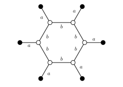
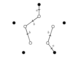
Let be a copy of . We define the cycle with pendant edges by the following vertex set and the edge set.
We define the nodes of by . In Figure 1 and Figure 2 a node is depicted as a black circle and an internal vertex is depicted as white circle.
Unless otherwise stated we use a weight of the cycle with pendant edges of the form
for two indeterminant and .
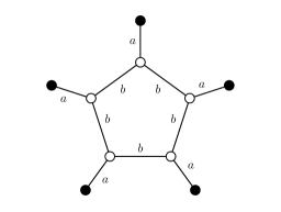
Remark 3.2.
A vertex of degree 1 is often called a pendant vertex, and the cycle with -pendant edges is also called the sun let graph with pendant vertices. See [Barrientos] or [Vernold] for example.
3.1. The non-oriented case
In our setting the weighted sum of is a two variable polynomial in and :
It can be seen that is a homogeneous polynomial of degree with . Our main result is the explicit description of using the Chebyshev polynomial of the first kind.
Definition 3.3.
For each positive integer the Chebyshev polynomial of the first kind is a polynomial satisfying the condition
for all .
Proposition 3.4.
The Chebyshev polynomial exists uniquely and can be computed by the recursive formula
The following is the main theorem.
Theorem 3.5.
To show Theorem 3.5 we introduce two lemmas below.
Lemma 3.6.
Let be a weighted graph with a decomposition . Let be the submatrix of the Laplacian matrix corresponding to the internal vertices . We have
Proof.
Let be the graph obtained from by identifying all nodes. Note that has only one node . One can see that there is a natural bijective between and . In particular we have . The Laplacian is a matrix of the form
By taking we have
by Theorem 2.4. ∎
Remark 3.7.
Lemma 3.8.
For a cycle with pendant edges we have
Proof.
We first see that
where is the cycle graph with and equipped with the constant weight . Then we have
As it is stated in [BrouwerHaemers, Section 1.4.3], one can see that eigenvalues of are
On the other hand the definition shows that the roots of are
and hence, two polynomials and have the same roots. Since the coefficient of in is one has
It implies that , and hence, we have
∎
3.2. The oriented case
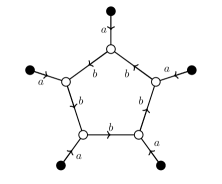
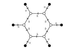
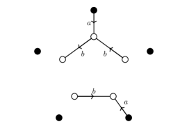
For each we fix an orientation of as follows. We fix the counter clockwise orientation of edges in and the orientation of pendant edges in such a way that . See Figure 3 and Figure 4
Let be the weighted oriented graph . We put
Theorem 3.9.
.
Proof.
Consider the oriented weighted graph by identifying all nodes in . We see that
and we use the oriented version of Lemma 3.6 so that we have
where
By the direct computation we have
∎
Remark 3.10.
Figure 5 is an example of the oriented rooted spanning forests, and Figure 6 is not. Theorem 3.9 can be obtained by a purely combinatorial argument without using the matrix tree theorem. In fact one can count that the number of oriented rooted spanning forests with internal edges is equal to the binomial coefficient , and hence, the formula
holds.
4. Corollaries and further discussions
Corollary 4.1.
The polynomial defined by
is a divisor of .
Proof.
We also introduce the polynomial
One can see that has two real roots when is even and one real root when is odd. In contrast we have shown in the proof of Lemma 3.8 that all roots of are real roots
We have the following corollary by [Brabden, Lemma 1.1].
Corollary 4.2.
Let be the coefficient of in . The sequence is log-concave, i.e., the inequality
holds for all . In particular they are unimodal, i.e., there exists such that
holds.
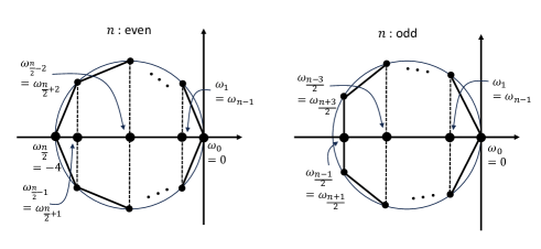
Remark 4.3.
The roots of are the real parts of for , which can be illustrated as shown in Figure 7 together with the circle and its inscribed -gon.
We have the following explicit computations, and these results suggest more detailed factorization of .
-
(1)
-
(2)
-
(3)
-
(4)
-
(5)
-
(6)
-
(7)
-
(8)
-
(9)
-
(10)
-
(11)
-
(12)
In fact the factorizations of and in into irreducible polynomials are shown in [HasegawaSugiyama]. To explain divisors of and we introduce auxiliary polynomials as follows. Let be the -th cyclotomic polynomial, i.e., the minimal polynomial of . Let be the minimal polynomial of .
Theorem 4.4 ([HasegawaSugiyama]).
We have the following factorizations of and in .
The above explicit computations include several divisibility, such as
By using Theorem 4.4, the following algebraic characterization of and including the divisibilities is shown.
Theorem 4.5 ([HasegawaSugiyama]).
Suppose that a sequence of polynomials of integer coefficients satisfies the following conditions for all .
-
(1)
-
(2)
is monic.
-
(3)
-
(4)
Then we have or for all .
More detailed algebraic properties will be shown in [HasegawaSugiyama], and graph theoretical interpretation of the divisibility will be discussed in the subsequent papers.