Baryogenesis in quantum fluctuation modified gravity

Abstract

We consider baryogenesis in quantum fluctuation modified gravity. We explore various forms (two are newly proposed here) of baryogenesis interaction and discuss the effect of these interaction terms on the baryon-to-entropy ratio during the radiation era of the expanding universe. We constrain the model parameters with the current observational data, implying that this modified gravity is capable to shed light on the issue of baryon asymmetry in a successful manner.

I Introduction

The problem of an excess of the matter over the anti-matter in the universe is one of the biggest mysteries of contemporary cosmology. This asymmetry is usually refer to the baryon asymmetry. The baryon number of the universe is precisely determined by observations, see for example, the latest result from Planck 2018 data Planck:2018vyg

$$\eta_{\rm{B}}\equiv\frac{n_{\rm{B}}}{s}=(8.70\pm 0.04)\times 10^{-11},$$ (1)

where $n_{\rm B}$ and $s$ are the baryon number density and the entropy density of the present universe, respectively. Studies suggest that the asymmetry between matter and anti-matter might occur during the radiation eras Riotto:1999yt ; Dine:2003ax ; Cline:2006ts . Sakharov suggested three conditions that are necessary to generate a baryon asymmetry Sakharov:1967dj : (i) non-conservation of baryon number; (ii) $\mathcal{C}$ and $\mathcal{CP}$ violation; (iii) deviation from thermal equilibrium. Various baryogenesis scenarios, such as GUT Baryogenesis Kolb:1996jt , Affleck-Dine Baryogenesis Affleck:1984fy ; Stewart:1996ai ; Yamada:2015xyr ; Akita:2017ecc , electroweak Baryogenesis Trodden:1998ym ; Morrissey:2012db , spontaneous Baryogenesis Takahashi:2003db ; DeSimone:2016ofp , baryogenesis through evaporation of primordial black holes Dolgov:1980gk or via spontaneous Lorentz violation Carroll:2005dj , and etc Alexander:2004us ; Mohanty:2005ud ; Abbott:1982hn ; Li:2004hh ; Hamada:2007vu ; Shiromizu:2004cb ; Cohen:1987vi ; Fukugita:1986hr ; Feng:2022gdz ; Li:2002wd ; Goodarzi:2023ltp ; Cado:2023gan ; RufranoAliberti:2023ywq , had been suggested to explain how there are more matter than antimatter in the universe.

Recently, a model had been suggested to generate the baryon number asymmetry by violation of $\mathcal{CPT}$, while the thermal equilibrium is maintained Cohen:1987vi . In Davoudiasl:2004gf , a dynamical violation of $\mathcal{CPT}$ (and also $\mathcal{CP}$) may give rise to the baryon asymmetry in thermal equilibrium during the expansion of the universe. The interaction responsible for $\mathcal{CP}$ violation is given by a coupling between the derivative of the Ricci scalar and the baryon current. This baryogenesis, called Gravitational baryogenesis, had been generalised to $f(R)$ theories Lambiase:2006dq , to Gauss-Bonnet gravity Odintsov:2016hgc , to $f(R,T)$ theories Baffou:2018hpe ; Nozari:2018ift ; Sahoo:2019pat , to $f(T)$ theory Oikonomou:2016jjh , to $f(R,L_{\rm{m}})$ theory Jaybhaye:2023lgr , and so on.

To explain the accelerated expansion of the universe, modified gravity is one popular attempt, such as $f(R)$ theories, Gauss-Bonnet gravity, and $f(R,T)$ theory. Recently, a type of modified gravity was proposed from Heisenberg’s nonperturbative quantization (Dzhunushaliev:2013nea, ; Dzhunushaliev:2015mva, ; Dzhunushaliev:2015hoa, ): if the metric can be decomposed as the sum of classical and quantum fluctuating parts, then the corresponding Einstein quantum gravity generates at the classical level modified gravity models with a non-minimal coupling between geometry and matter Yang:2015jla . This idea has been realized in some specific models Yang:2015jla ; Liu:2016qfx ; Bernardo:2021ynf ; Chen:2021oal ; Lima:2023qdv . Some of these modified gravity had been applied to black hole physics Yang:2020lxv and to Friedmann-Lemaitre-Robertson-Walker geometries Yang:2015jla ; Liu:2016qfx ; Bernardo:2021ynf ; Haghani:2021iqe ; Chen:2021oal . Since the quantum fluctuations of metric will lead to modified gravitational field equations, it may cause the symmetry breaking between matter and anti-matter. In this paper, we will investigate this issue in the framework of quantum fluctuation modified gravity (QFMG) proposed in Yang:2015jla . The results show that the QFMG may provide a possible solution to the problem of baryon asymmetry.

The paper is organized as follows. In the next Section, we will briefly review the QFMG proposed in Yang:2015jla . In Sec. III, we will discuss the baryon asymmetry in this modified gravity. Finally, we will briefly summarize and discuss our results in section IV. For numerical calculations and graphs, the physical constants take the following values: $G/c^{2}=7.425\times 10^{-29}$ cm/g, $c=2.998\times 10\times{10}$ cm/s, $\hbar=6.58\times 10^{-16}$ eV s, $k_{\rm B}=1.381\times 10^{-16}$ erg/K.

II Quantum fluctuation modified gravity

If the metric operator can be decomposed into a sum of a classical metric $g_{\mu\nu}$ and a fluctuating part $\widehat{\delta g}_{\mu\nu}$ (Dzhunushaliev:2013nea, ), and $\hat{g}_{\mu\nu}=g_{\mu\nu}+\widehat{\delta g}_{\mu\nu}$, assuming $\langle\delta\hat{g}_{\mu\nu}\rangle\neq 0$ for any quantum state and ignoring high order fluctuations, the quantum Einstein-Hilbert Lagrangian $L_{\hat{g}}=\frac{1}{2k^{2}}\sqrt{-\hat{g}}\hat{R}$ can be expanded as

$$L_{\hat{g}}=L_{\hat{g}}(g+\delta\hat{g})\approx L_{g}(g)+\frac{\delta L_{g}}{\delta g^{\mu\nu}}\widehat{\delta g}^{\mu\nu}.$$ (2)

Hereafter $k^{2}=8\pi G$ and we take $c=\hbar=k_{B}=1$ with $k_{\rm{B}}$ the Boltzmann constant. Since $\left\langle\frac{\delta L_{g}}{\delta g^{\mu\nu}}\widehat{\delta g}^{\mu\nu}\right\rangle=\frac{\delta L_{g}}{\delta g^{\mu\nu}}\langle\widehat{\delta g}^{\mu\nu}\rangle=\sqrt{-g}G_{\mu\nu}\langle\widehat{\delta g}^{\mu\nu}\rangle$ Dzhunushaliev:2013nea , the expectation value of Lagrangian (2) has the form

$$\langle L_{\hat{g}}\rangle\approx\frac{1}{2k^{2}}\sqrt{-g}\big{[}R+G_{\mu\nu}\langle\delta\hat{g}^{\mu\nu}\rangle\big{]},$$ (3)

Similarly, the quantum Lagrange density $L^{\hat{g}}_{\rm m}$ can be expanded as follows

$$L^{\hat{g}}_{\rm m}(g+\delta\hat{g})\approx\sqrt{-g}L_{\rm m}(g)+\frac{\delta\sqrt{-g}L_{\rm m}}{\delta g^{\mu\nu}}\widehat{\delta g}^{\mu\nu}.$$ (4)

With the aforementioned assumptions, the expectation value of the quantum Lagrange density (4) is given by (Dzhunushaliev:2013nea, )

$$\langle L^{\hat{g}}_{\rm m}(g+\delta\hat{g})\rangle\approx\sqrt{-g}\big{[}L_{\rm m}-\frac{1}{2}T_{\mu\nu}\langle\delta\hat{g}^{\mu\nu}\rangle\big{]},$$ (5)

where $T_{\mu\nu}=-2\delta(\sqrt{-g}L_{\rm m})/(\sqrt{-g}\delta g^{\mu\nu})$ is the energy-momentum tensor, Then the modified Lagrangian density can be written as

$$L=\frac{1}{2k^{2}}\sqrt{-g}\big{[}R+G_{\mu\nu}\langle\delta\hat{g}^{\mu\nu}\rangle\big{]}+\sqrt{-g}\big{[}L_{\rm m}-\frac{1}{2}T_{\mu\nu}\langle\delta\hat{g}^{\mu\nu}\rangle\big{]}.$$ (6)

In Yang:2015jla , a simple case $\langle\delta\hat{g}^{\mu\nu}\rangle=\alpha g^{\mu\nu}$ with $\alpha$ a constant has been considered, and the Lagrangian density (6) becomes as

$$L=L_{\rm mg}+L_{\rm mm}=\frac{1}{2k^{2}}\sqrt{-g}(1-\alpha)R+\sqrt{-g}[L_{\rm m}-\frac{1}{2}\alpha T],$$ (7)

where $T=g_{\mu\nu}T^{\mu\nu}$ is the trace of the energy-momentum tensor. Here we assume that the quantum fluctuation is less than the classical part of the metric operator: $|\alpha|<0$. Varying the Lagrangian density (6) with respect to $g^{\mu\nu}$ and assuming $\delta g_{\mu\nu}=0$ on the boundary, we obtain the gravitational field equations Yang:2015jla

$$R_{\mu\nu}-\frac{1}{2}g_{\mu\nu}R=\frac{2k^{2}}{1-\alpha}\left[\frac{1}{2}(1+\alpha)T_{\mu\nu}-\frac{1}{4}\alpha g_{\mu\nu}T+\frac{1}{2}\alpha\theta_{\mu\nu}\right],$$ (8)

where $\theta_{\mu\nu}=g^{\alpha\beta}\delta T_{\alpha\beta}/\delta g^{\mu\nu}$ and $\theta=g_{\mu\nu}\theta^{\mu\nu}$, for detail see Yang:2015jla . For convenience, we call $\theta_{\mu\nu}$ as energy-momentum induced tensor. We observe that the gravitational constant $G$ and the energy-momentum tensor are modified due to the quantum fluctuation of the metric. Since $R=-k^{2}[T+\alpha\theta/(1-\alpha)]$, the gravitational field equations (8) can be rewritten as Yang:2015jla

$$R_{\mu\nu}=\frac{2k^{2}}{1-\alpha}\left[\frac{1}{2}(1+\alpha)T_{\mu\nu}-\frac{1}{4}g_{\mu\nu}T+\frac{1}{2}\alpha\theta_{\mu\nu}-\frac{1}{4}\alpha g_{\mu\nu}\theta\right].$$ (9)

Thinking of $\nabla_{\nu}G^{\mu\nu}=0$, we derive the equation for the divergence of the stress-energy tensor $T_{\mu\nu}$ Yang:2015jla

$$\nabla^{\nu}T_{\mu\nu}=\frac{1}{1+\alpha}\left[\frac{1}{2}\alpha\nabla_{\mu}T-\alpha\nabla^{\nu}\theta_{\mu\nu}\right].$$ (10)

In other words, if taking into account of quantum fluctuations, the stress-energy tensor are not conserved quantities any more. Discussions about the nonconservation of stress-energy tensor can be found in (Bertolami:2008ab, ; Harko:2008qz, ; Bisabr:2012tg, ; Minazzoli:2013bva, ). As pointed out in Liu:2016qfx ; Yang:2020lxv , the Lagrangian density (6) suggests an possible equivalent microscopic quantum description of the matter creation processes in $f(R,T)$ or $f(R,L_{\rm{m}})$ gravity. Such a description may shed some lights on the physical mechanisms leading to particle generation via gravity and matter geometry coupling.

III Baryogenesis in quantum fluctuation modified gravity

Consider a homogeneous and isotropic Friedmann-Lemaître-Robertson-Walker (FLRW) universe

$$ds^{2}=dt^{2}-a^{2}(t)\left[\frac{dr^{2}}{1+Kr^{2}}+r^{2}(d\theta^{2}+\sin^{2}\theta d\phi^{2})\right],$$ (11)

where $a$ is the scalar factor. The spatial curvature constant $K=+1$, 0, and $-1$ correspond to a closed, flat, and open universe, respectively. And suggest a perfect fluid specified by the energy-momentum tensor

$$T_{\mu\nu}=(\rho+p)u_{\mu}u_{\nu}-g_{\mu\nu}p.$$ (12)

where the fluid 4-velocity fulfil the condition $u^{\mu}u_{\mu}=1$. Taking the Lagrangian for matter as $L_{\rm m}=-p$, we have from the variation of the energy-momentum tensor of a perfect fluid

$$\theta_{\mu\nu}=-2T_{\mu\nu}-g_{\mu\nu}p.$$ (13)

With $T=\rho-3p$ and $\theta=-2T-4p=-2(\rho-p)$, the $\mu\nu=00$ component of Eq. (9) is Yang:2015jla

$$\frac{\ddot{a}}{a}=-\frac{1}{3}\frac{k^{2}}{2(1-\alpha)}\big{[}\rho+(3-4\alpha)p\big{]},$$ (14)

and the equations $\mu\nu=00$ and $\mu\nu=11$ together yield Yang:2015jla

$$H^{2}+\frac{K}{a^{2}}=\frac{1}{3}\frac{k^{2}}{2(1-\alpha)}\left[(2-3\alpha)\rho+\alpha p\right].$$ (15)

For a spatial flat FLRW spacetime, Eqs. (15) and (14) become Yang:2015jla

$$H^{2} = \frac{k^{2}}{3}\left[\frac{2-(3-w)\alpha}{2-2\alpha}\right]\rho,$$ (16)

$$\dot{H}+H^{2} = \frac{\ddot{a}}{a}=-\frac{k^{2}}{6}\left[\frac{1+(3-4\alpha)w}{1-\alpha}\right]\rho,$$ (17)

with $w=p/\rho$. Contracting these two equations, we have

$$\dot{H}+\frac{3(1-\alpha)\left(1+\omega\right)}{2+\alpha\left(\omega-3\right)}H^{2}=0.$$ (18)

Solving this equation, we get

$$H=\frac{\lambda}{t},$$ (19)

where

$$\lambda=\frac{2-\left(3-w\right)\alpha}{3\left(1-\alpha\right)\left(1+w\right)}.$$ (20)

Substituting Eq. (19) into Eq. (16), yields

$$\rho=\rho_{0}t^{-2},$$ (21)

where

$$\rho_{0}=\frac{2[2-(3-\omega)\alpha]}{3k^{2}(1-\alpha)(1+\omega)^{2}}.$$ (22)

Assuming that he universe evolves slowly from an equilibrium state to an equilibrium state, the energy density links to the temperature $\mathcal{T}$ as

$$\rho=\frac{\pi^{2}}{30}g_{*}\mathcal{T}^{4},$$ (23)

where $g_{*}$ denotes the number of the degrees of freedom of the effectively massless particles. Using this equation and the energy density (21), we find the decoupling time as a function of decoupling temperature $\mathcal{T}_{\rm{D}}$ as

$$t_{\rm{D}}=\left(\frac{30\rho_{0}}{\pi^{2}g_{*}}\right)^{\frac{1}{2}}\mathcal{T}_{\rm{D}}^{-2}.$$ (24)

With this equation and a certain baryogenesis interaction term, we can discuss whether this mechanism generates baryon asymmetry during the expansion of the universe.

III.1 Coupling of the baryon current with Ricci scalar

Figure 1: The cutoff scale $M_{*}$ as a function of the parameter $\alpha$ in the coupling model $J_{\mu}\partial^{\mu}R$ with $w=1/3$, $g_{\rm{b}}=1$, $g_{*}=106$, $\mathcal{T}_{\rm{D}}=2\times 10^{16}$ GeV, and $\eta_{\rm{B}}=10^{-10}$ K/J, $\eta_{\rm{B}}=10^{-11}$ K/J, $\eta_{\rm{B}}=10^{-12}$ K/J respectively.

	$\alpha=-0.01$	$\alpha=-0.05$	$\alpha=-0.1$	$\alpha=-0.5$
$M_{*}$ GeV	$2.393\times 10^{17}$	$5.231\times 10^{17}$	$7.202\times 10^{17}$	$1.353\times 10^{18}$

Table 1: Some values of the cutoff scale $M_{*}$ in the coupling model $J_{\mu}\partial^{\mu}R$ with $\eta_{\rm{B}}=8.70\times 10^{-11}$ K/J.

Figure 2: The decoupling temperature $T_{\rm{D}}$ as a function of the parameter $\alpha$ in the coupling model $J_{\mu}\partial^{\mu}R$ with $w=1/3$, $g_{\rm{b}}=1$, $g_{*}=106$, $M_{*}=\times 10^{19}$ GeV, and $\eta_{\rm{B}}=10^{-10}$ K/J, $\eta_{\rm{B}}=10^{-11}$ K/J, $\eta_{\rm{B}}=10^{-12}$ K/J respectively.

	$\alpha=-0.01$	$\alpha=-0.05$	$\alpha=-0.1$	$\alpha=-0.5$
$\mathcal{T}_{\rm{D}}$ GeV	$1.033\times 10^{21}$	$7.551\times 10^{20}$	$6.644\times 10^{20}$	$5.163\times 10^{20}$

Table 2: Some values of the decoupling temperature $\mathcal{T}_{\rm{D}}$ in the coupling model $J_{\mu}\partial^{\mu}R$ with $\eta_{\rm{B}}=8.70\times 10^{-11}$ K/J.

We first consider the possibility that the baryon current couplings with Ricci scalar. The interaction between the derivative of the Ricci scalar $R$ and the baryon-number current $J_{\mu}$ breaks $\mathcal{CPT}$ dynamically in the expansion of the universe. The $\mathcal{CP}$-violating interaction term is given by

$$-\frac{1}{M_{*}^{2}}\int d^{4}x\sqrt{-g}J^{\mu}\partial_{\mu}R,$$ (25)

where $J^{\mu}$ is the baryonic matter current and $M_{*}$ is the cutoff scale of underlying effective theory. After the temperature of the universe drops below the critical temperature $\mathcal{T}_{\rm{D}}$, the baryon-to-entropy ratio in the expansion of universe becomes Davoudiasl:2004gf

$$\frac{n_{\rm{B}}}{s}\simeq-\frac{15g_{\rm{b}}}{4\pi^{2}g_{*}}\frac{\dot{R}}{M_{*}^{2}\mathcal{T}_{\rm{D}}}.$$ (26)

$\eta_{\rm{B}}$ has a dimension of (K/J) in SI units. For a flat FLRW metric, the Ricci scalar is given by

$$R=-6\left(\dot{H}+2H^{2}\right)=\frac{6\lambda(2\lambda-1)}{t^{2}},$$ (27)

So the time derivative of the Ricci scalar is

$$\dot{R}=\frac{12\lambda(2\lambda-1)}{t^{3}}=\frac{12\lambda(2\lambda-1)}{c^{2}t^{3}}.$$ (28)

Inserting Eqs. (24) and (28) into Eq. (26), we obtain the baryon asymmetry factor as

$$\eta_{\rm{B}}\equiv\frac{n_{\rm{B}}}{s}\simeq\left(\frac{648}{5}\right)^{\frac{1}{2}}\frac{g_{\rm b}g^{1/2}_{*}\pi^{5/2}\lambda(2\lambda-1)}{M_{*}^{2}}\left[\frac{(1-\alpha)(1+w)^{2}}{2-(3-w)\alpha}\right]^{\frac{3}{2}}\mathcal{T}_{D}^{5}$$ (29)

Hereafter we denote $n_{\rm{B}}/s$ as $\eta_{\rm{B}}$ for convenience. If $\lambda\neq 1/2$ (i.e. $\alpha\neq 0$), this equation shows that the resulting baryon-to-entropy ratio is non-zero even in radiation dominated era ($w=1/3$). Thinking of the conditions: $|\alpha|<0$ and $\eta_{\rm{B}}>0$, we have $-1<\alpha<0$ from Eq. (29) for $w=1/3$. Assuming that $g_{\rm{b}}\simeq\mathcal{O}(1)$ and $g_{*}\simeq 106$, there are still three parameters needed to be determined: $\alpha$, $M_{*}$, and $\mathcal{T}_{\rm{D}}$. We consider two possible choices: taking $M_{*}\sim m_{\rm{p}}=10^{19}$ GeV but keep $\mathcal{T}_{\rm{D}}$ as a free parameter, or taking $\mathcal{T}_{\rm{D}}=M_{I}=2\times 10^{16}$ GeV with $M_{I}$ the upper bound for tensor mode fluctuation constraints on the inflationary scale but keep $M_{*}$ as a free parameter.

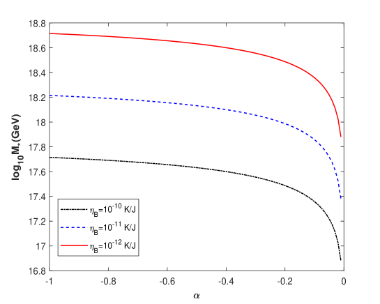
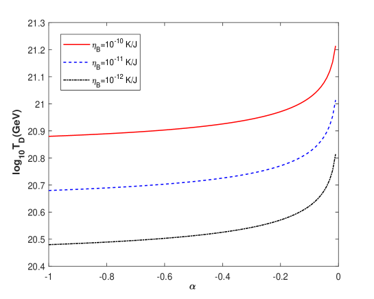
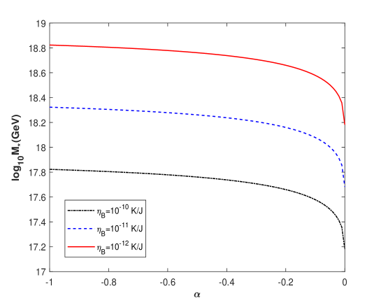
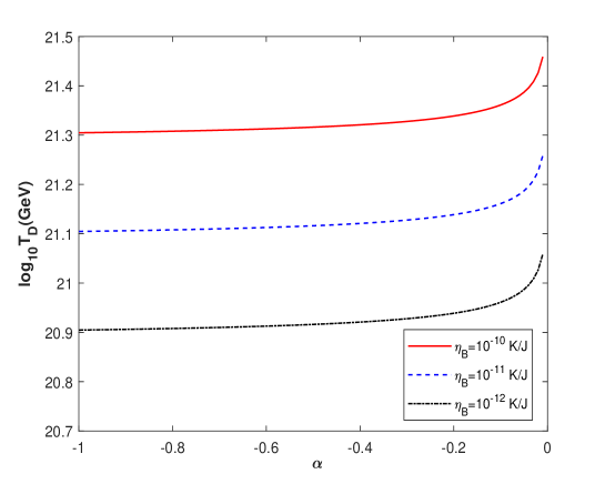
For this coupling model, $J_{\mu}\partial^{\mu}R$, we plot in figure 1 the cutoff scale $M_{*}$ as a function of the parameter $\alpha$ with $\mathcal{T}_{\rm{D}}=2\times 10^{16}$ GeV, and $\eta_{\rm{B}}=10^{-10}$ K/J, $\eta_{\rm{B}}=10^{-11}$ K/J, $\eta_{\rm{B}}=10^{-12}$ K/J respectively. We can observe that the parameter $M_{*}$ decreases as the parameter $\alpha$ increasing and $M_{*}<10^{18.8}$ GeV. In table 1, we present some specific values of the parameter $M_{*}$ for some given values of the parameter $\alpha$. In figure 2, we plot the decoupling temperature $\mathcal{T}_{\rm{D}}$ as a function of the parameter $\alpha$ with $M_{*}=10^{19}$ GeV, and $\eta_{\rm{B}}=10^{-10}$ K/J, $\eta_{\rm{B}}=10^{-11}$ K/J, $\eta_{\rm{B}}=10^{-12}$ K/J respectively. We observe that the parameter $\mathcal{T}_{\rm{D}}$ increases as the parameter $\alpha$ increasing and $\mathcal{T}_{\rm{D}}>10^{20.4}$ Gev. In table 2, some specific values of the parameter $\mathcal{T}_{\rm{D}}$ are presented for some given values of the parameter $\alpha$.

III.2 Coupling of the baryon current with energy-momentum induced tensor

Figure 3: The cutoff scale $M_{*}$ as a function of the parameter $\alpha$ in the coupling model $-J_{\mu}\partial^{\mu}\theta$ with $w=1/3$, $g_{\rm{b}}=1$, $g_{*}=106$, $\mathcal{T}_{\rm{D}}=2\times 10^{16}$ GeV, and $\eta_{\rm{B}}=10^{-10}$ K/J, $\eta_{\rm{B}}=10^{-11}$ K/J, $\eta_{\rm{B}}=10^{-12}$ K/J respectively.

	$\alpha=-0.5$	$\alpha=-0.1$	$\alpha=0.1$	$\alpha=0.5$
$M_{*}$ GeV	$4.677\times 10^{17}$	$4.766\times 10^{17}$	$4.848\times 10^{17}$	$5.314\times 10^{17}$

Table 3: Some values of the cutoff scale $M_{*}$ in the coupling model $-J_{\mu}\partial^{\mu}\theta$ with $\eta_{\rm{B}}=8.70\times 10^{-11}$ K/J.

Figure 4: The decoupling temperature $\mathcal{T}_{\rm{D}}$ as a function of the parameter $\alpha$ in the coupling model $-J_{\mu}\partial^{\mu}\theta$ with $w=1/3$, $g_{\rm{b}}=1$, $g_{*}=106$, $M_{*}=\times 10^{19}$ GeV, and $\eta_{\rm{B}}=10^{-10}$ K/J, $\eta_{\rm{B}}=10^{-11}$ K/J, $\eta_{\rm{B}}=10^{-12}$ K/J respectively.

	$\alpha=-0.5$	$\alpha=-0.1$	$\alpha=0.1$	$\alpha=0.5$
$\mathcal{T}_{\rm{D}}$ GeV	$7.901\times 10^{20}$	$7.842\times 10^{20}$	$7.789\times 10^{20}$	$7.508\times 10^{20}$

Table 4: Some values of the decoupling temperature $\mathcal{T}_{\rm{D}}$ in the coupling model $-J_{\mu}\partial^{\mu}\theta$ with $\eta_{\rm{B}}=8.70\times 10^{-11}$ K/J.

In some literatures, the baryogenesis interaction term, $J_{\mu}\partial^{\mu}T$, was considered. However, since $T=\rho-3p=(1-3w)\rho$, this interaction term will not contribute to the baryon asymmetry in the radiation dominated era. Here we consider a new baryogenesis interaction term which is given by

$$-\frac{1}{M_{*}^{2}}\int d^{4}x\sqrt{-g}J^{\mu}\partial_{\mu}\theta.$$ (30)

For this case, the baryon-to-entropy ratio can be defined as

$$\frac{n_{\rm{B}}}{s}\simeq-\frac{15g_{\rm{b}}}{4\pi^{2}g_{*}}\frac{\dot{\theta}}{M_{*}^{2}\mathcal{T}_{\rm{D}}}.$$ (31)

From Eq. (13), and combining with Eq. (21), one can easily get

$$\theta=-2(\rho-p)=-2(1-w)\rho=-2(1-w)\rho_{0}t^{-2}.$$ (32)

Combining this equation with Eq. (24), we derive

$$\eta_{\rm{B}}=\frac{n_{\rm{B}}}{s}=\left(\frac{1}{10}\right)^{\frac{1}{2}}\frac{g_{\rm b}g^{1/2}_{*}\pi^{3/2}(1-w)}{M_{*}^{2}}\left[\frac{(1-\alpha)(1+w)^{2}}{2-(3-w)\alpha}\right]^{\frac{1}{2}}\mathcal{T}_{D}^{5}$$ (33)

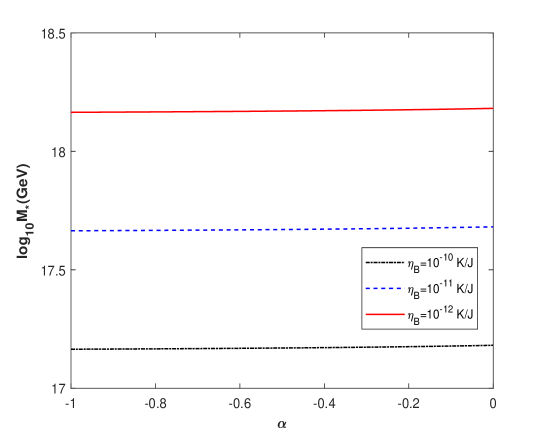
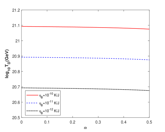
For $w=1/3$, the conditions $|\alpha|<0$ and $\eta_{\rm{B}}>0$ imply that $-1<\alpha<3/4$ and $\alpha\neq 0$. For this coupling model $-J_{\mu}\partial^{\mu}\theta$, we plot in figure 3 the cutoff scale $M_{*}$ as a function of the parameter $\alpha$ with $\mathcal{T}_{\rm{D}}=2\times 10^{16}$ GeV, and $\eta_{\rm{B}}=10^{-10}$ K/J, $\eta_{\rm{B}}=10^{-11}$ K/J, $\eta_{\rm{B}}=10^{-12}$ K/J respectively. We observe that the parameter $M_{*}$ increases very slowly as the parameter $\alpha$ increasing and $M_{*}>10^{17}$ GeV. In table 3, we present some specific values of the parameter $M_{*}$ for some given values of the parameter $\alpha$. In figure 4, the decoupling temperature $\mathcal{T}_{\rm{D}}$ as a function of the parameter $\alpha$ is plotted with $M_{*}=10^{19}$ GeV, and $\eta_{\rm{B}}=10^{-10}$ K/J, $\eta_{\rm{B}}=10^{-11}$ K/J, $\eta_{\rm{B}}=10^{-12}$ K/J respectively. We can observe that the parameter $\mathcal{T}_{\rm{D}}$ decreases very slowly as the parameter $\alpha$ increasing and $\mathcal{T}_{\rm{D}}<10^{21.1}$ Gev. In table 2, some specific values of the parameter $\mathcal{T}_{\rm{D}}$ are presented for some given values of the parameter $\alpha$.

III.3 A generalized baryogenesis interaction term

Now consider a more general baryogenesis interaction term

$$-\frac{1}{M^{2}_{*}}\int d^{4}x\sqrt{-g}J^{\mu}\partial_{\mu}F(R,\theta)\ ,\\$$ (34)

where $F(R,\theta)$ is any function of $R$ and $\theta$. The baryon to entropy ratio can be calculated as

$$\frac{n_{\rm{B}}}{s}=-\frac{15g_{b}}{4\pi^{2}g_{*}}\frac{\dot{R}F_{R}+\dot{\theta}F_{\theta}}{M_{*}^{2}\mathcal{T}_{D}}\ .\\$$ (35)

where $F_{R}\equiv dF/dR$ and $F_{\theta}\equiv dF/d\theta$. Using Eqs. (29) and (33), we obtain

$$\frac{n_{\rm{B}}}{s}\simeq\left\{\left(\frac{648}{5}\right)^{\frac{1}{2}}\frac{g_{\rm b}g^{\frac{1}{2}}_{*}\pi^{\frac{5}{2}}\lambda(2\lambda-1)}{M_{*}^{2}}\left[\frac{(1-\alpha)(1+w)^{2}}{2-(3-w)\alpha}\right]^{\frac{3}{2}}F_{R}+\left(\frac{1}{10}\right)^{\frac{1}{2}}\frac{g_{\rm b}g^{\frac{1}{2}}_{*}\pi^{\frac{3}{2}}(1-w)}{M_{*}^{2}}\left[\frac{(1-\alpha)(1+w)^{2}}{2-(3-w)\alpha}\right]^{\frac{1}{2}}F_{\theta}\right\}\mathcal{T}_{D}^{5}.$$ (36)

. Since $F(R,\theta)$ is unknown, here we consider a simple case: $F(R,\theta)=R+\theta$. Then from (36), we have

$$\frac{n_{\rm{B}}}{s}\simeq\left\{\left(\frac{648}{5}\right)^{\frac{1}{2}}\frac{g_{\rm b}g^{\frac{1}{2}}_{*}\pi^{\frac{5}{2}}\lambda(2\lambda-1)}{M_{*}^{2}}\left[\frac{(1-\alpha)(1+w)^{2}}{2-(3-w)\alpha}\right]^{\frac{3}{2}}+\left(\frac{1}{10}\right)^{\frac{1}{2}}\frac{g_{\rm b}g^{\frac{1}{2}}_{*}\pi^{\frac{3}{2}}(1-w)}{M_{*}^{2}}\left[\frac{(1-\alpha)(1+w)^{2}}{2-(3-w)\alpha}\right]^{\frac{1}{2}}\right\}\mathcal{T}_{D}^{5}.$$ (37)

. For this coupling model $J_{\mu}(\partial^{\mu}R+\partial^{\mu}\theta)$, we plot in figure 5 the cutoff scale $M_{*}$ as a function of the parameter $\alpha$ with $\mathcal{T}_{\rm{D}}=2\times 10^{16}$ GeV, and $\eta_{\rm{B}}=10^{-10}$ K/J, $\eta_{\rm{B}}=10^{-11}$ K/J, $\eta_{\rm{B}}=10^{-12}$ K/J respectively. We observe that the parameter $M_{*}$ decreases as the parameter $\alpha$ increasing and $M_{*}<10^{19}$ GeV. In table 5, some specific values of the parameter $M_{*}$ are presented for some given values of the parameter $\alpha$. In figure 6, we plot the decoupling temperature $\mathcal{T}_{\rm{D}}$ as a function of the parameter $\alpha$ with $M_{*}=10^{12}$ GeV, and $\eta_{\rm{B}}=10^{-10}$ K/J, $\eta_{\rm{B}}=10^{-11}$ K/J, $\eta_{\rm{B}}=10^{-12}$ K/J respectively. We can observe that the parameter $\mathcal{T}_{\rm{D}}$ increases as the parameter $\alpha$ increasing and $\mathcal{T}_{\rm{D}}>10^{20.9}$ Gev. In table 6, some specific values of the parameter $\mathcal{T}_{D}$ are presented for some given values of the parameter $\alpha$.

Figure 5: The cutoff scale $M_{*}$ as a function of the parameter $\alpha$ in the coupling model $J_{\mu}(\partial^{\mu}R+\partial^{\mu}\theta)$ with $w=1/3$, $g_{\rm{b}}=1$, $g_{*}=106$, $\mathcal{T}_{\rm{D}}=2\times 10^{16}$ GeV, and $\eta_{\rm{B}}=10^{-10}$ K/J, $\eta_{\rm{B}}=10^{-11}$ K/J, $\eta_{\rm{B}}=10^{-12}$ K/J respectively.

	$\alpha=-0.01$	$\alpha=-0.05$	$\alpha=-0.1$	$\alpha=-0.5$
$M_{*}$ GeV	$7.2\times 10^{17}$	$1.003\times 10^{18}$	$1.198\times 10^{18}$	$1.824\times 10^{18}$

Table 5: Some values of the cutoff scale $M_{*}$ in the coupling model $J_{\mu}(\partial^{\mu}R+\partial^{\mu}\theta)$ with $\eta_{\rm{B}}=8.70\times 10^{-11}$ K/J.

Figure 6: The decoupling temperature $T_{D}$ as a function of the parameter $\alpha$ in the coupling model $J_{\mu}(\partial^{\mu}R-\partial^{\mu}\theta)$ with $w=1/3$, $g_{\rm{b}}=1$, $g_{*}=106$, $M_{*}=\times 10^{19}$ GeV, and $\eta_{\rm{B}}=10^{-10}$ K/J, $\eta_{\rm{B}}=10^{-11}$ K/J, $\eta_{\rm{B}}=10^{-12}$ K/J respectively.

	$\alpha=-0.01$	$\alpha=-0.05$	$\alpha=-0.1$	$\alpha=-0.5$
$\mathcal{T}_{\rm{D}}$ GeV	$1.815\times 10^{21}$	$1.539\times 10^{21}$	$1.449\times 10^{21}$	$1.307\times 10^{21}$

Table 6: Some values of the decoupling temperature $\mathcal{T}_{\rm{D}}$ in the coupling model $J_{\mu}(\partial^{\mu}R-\partial^{\mu}\theta)$ with $\eta_{\rm{B}}=8.70\times 10^{-11}$ K/J.

IV Conclusions and discussions

We have discussed baryogenesis scenario in quantum fluctuation modified gravity. We have explored that how this modified gravity is capable to explain the observed asymmetry between matter and antimatter. We have considered three forms (two are newly proposed here) of baryogenesis interaction and investigate the effects of these interaction terms on the baryon-to-entropy ratio during the radiation era of the expanding universe. We have plotted the cutoff scale or the decoupling temperature as a function of the model parameter and have presented some values of the cutoff scale or the decoupling temperature for some given values of the baryon-to-entropy ratio in these coupling models. We have shown that the current observational value of the baryon-to-entropy ratio can be obtained for large set of parameters of the models as well as the decoupling temperature, and the characteristic cutoff scale.