Abstract

A significant challenge in multi-objective reinforcement learning is obtaining a Pareto front of policies that attain optimal performance under different preferences. We introduce Iterated Pareto Referent Optimisation (IPRO), a principled algorithm that decomposes the task of finding the Pareto front into a sequence of single-objective problems for which various solution methods exist. This enables us to establish convergence guarantees while providing an upper bound on the distance to undiscovered Pareto optimal solutions at each step. Empirical evaluations demonstrate that IPRO matches or outperforms methods that require additional domain knowledge. By leveraging problem-specific single-objective solvers, our approach also holds promise for applications beyond multi-objective reinforcement learning, such as in pathfinding and optimisation.

1 Introduction

Agents operating in sequential decision-making problems often have multiple and conflicting objectives to optimise. Controlling a water reservoir, for example, involves a complex trade-off between environmental, economic and social factors (Castelletti et al., 2013). Given that there is usually no single policy that maximises all objectives simultaneously, it is common to compute a set of candidate optimal policies. This set is subsequently presented to a decision maker who selects their preferred policy from it. This approach has multiple advantages such as systematically exploring the space of trade-offs and empowering a decision-maker to examine the outcomes of their decisions with respect to their objectives (Hayes et al., 2022). A solution set that is often considered in multi-objective reinforcement learning (MORL) is the Pareto front, consisting of all policies leading to non-dominated expected returns.

When assuming decision-makers utilise a linear scalarisation function or allow for stochastic policies, the resulting Pareto front is guaranteed to be convex (Roijers & Whiteson, 2017; Lu et al., 2023), enabling the application of effective solution methods (Yang et al., 2019; Xu et al., 2020). However, when deterministic policies are preferred for safety, accountability or interpretability reasons, the resulting Pareto front may instead be irregularly shaped. Algorithms addressing this setting have been elusive, with successful solutions limited to purely deterministic environments (Reymond et al., 2022).

To address this challenge, we propose a novel MORL algorithm, Iterated Pareto Referent Optimisation (IPRO), that learns the Pareto front by decomposing this task into a sequence of single-objective problems. In multi-objective optimisation (MOO), decomposition stands as a successful paradigm for computing a Pareto front. This approach makes use of efficient single-objective methods to solve the decomposed problems, thereby also establishing a robust connection between advancements in multi-objective and single-objective methods (Zhang & Li, 2007). Notably, existing MORL algorithms dealing with a convex Pareto front frequently employ decomposition and rely on single-objective RL algorithms to solve the resulting problems (Lu et al., 2023; Alegre et al., 2023).

Contributions. IPRO learns the Pareto front for diverse policy classes by decomposing this task into learning a sequence of Pareto optimal policies. We show that learning any Pareto optimal policy corresponds to a distinct single-objective problem for which principled solution methods can be derived. Combining these, we guarantee convergence to the Pareto front and provide bounds on the distance to undiscovered solutions at each iteration. Furthermore, we propose a practical extension which enables a single network to encompass all Pareto optimal policies. While IPRO applies to any policy class, we specifically demonstrate its effectiveness for deterministic policies, a class lacking general methods. When comparing IPRO to algorithms which require additional assumptions on the structure of the Pareto front or the underlying environment, we find that it matches or outperforms them, thereby showcasing its efficacy.

2 Related work

When learning a single policy in MOMDPs, as is necessary in IPRO, conventional methods often adapt single-objective RL algorithms. For example, Siddique et al. (2020) extend DQN, A2C and PPO to learn a fair policy by optimising the generalised Gini index of the expected returns. Reymond et al. (2023) extend this to general non-linear functions and establish a policy gradient theorem for this setting. When maximising a concave function of the expected returns, efficient methods exist which guarantee global convergence (Zhang et al., 2020; Zahavy et al., 2021; Geist et al., 2022).

To learn a Pareto front in deterministic MOMDPs, Reymond et al. (2022) train a neural network to predict deterministic policies for various desired trade-off points. Related to our approach, Van Moffaert et al. (2013) learn deterministic policies on the Pareto front by decomposing the problem into a sequence of single-objective problems using the Chebyshev scalarisation function. However, their method has no theoretical guarantees and does not extend to settings with continuous state or action spaces. When the Pareto front is convex, many techniques rely on the fact that the overall problem can be decomposed into single-objective problems where the scalar reward is a convex combination of the original reward vector (Yang et al., 2019; Alegre et al., 2023). Furthermore, Lu et al. (2023) demonstrate that, in this setting, it is possible to add a strongly concave term to the reward function and induce a sequence of single-objective problems with different weights.

In MOO, a related methodology has been proposed by Legriel et al. (2010) to obtain approximate Pareto fronts. Their approach iteratively proposes queries to an oracle and uses the return value to trim sections from the search space. In contrast, we introduce an alternative technique for query selection that ensures convergence to the exact Pareto front in the limit. Moreover, we contribute novel results specifically tailored to multi-objective Markov decision processes and reinforcement learning.

3 Preliminaries

Pareto dominance. For two vectors ${\bm{v}},{\bm{v}}^{\prime}\in\mathbb{R}^{d}$ we say that ${\bm{v}}$ Pareto dominates ${\bm{v}}^{\prime}$, denoted ${\bm{v}}\succ{\bm{v}}^{\prime}$, when $\forall j\in\{1,\dotsc,d\}:{\bm{v}}_{j}\geq{\bm{v}}^{\prime}_{j}$ and ${\bm{v}}_{j}>{\bm{v}}^{\prime}_{j}$ for at least one $j$. When dropping the strict condition, we write ${\bm{v}}\succeq{\bm{v}}^{\prime}$. We say that ${\bm{v}}$ strictly Pareto dominates ${\bm{v}}^{\prime}$, denoted ${\bm{v}}>{\bm{v}}^{\prime}$ when $\forall j\in\{1,\dotsc,d\}:{\bm{v}}_{j}>{\bm{v}}^{\prime}_{j}$. When a vector is not pairwise (strictly) Pareto dominated, it is (strictly) Pareto optimal. Finally, a vector is weakly Pareto optimal whenever there is no other vector that strictly Pareto dominates it.

In multi-objective decision-making, Pareto optimal vectors are relevant when considering decision-makers with monotonically increasing utility functions. In particular, if ${\bm{v}}\succ{\bm{v}}^{\prime}$, then ${\bm{v}}$ will be preferred over ${\bm{v}}^{\prime}$ by all decision-makers. The set of all pairwise Pareto non-dominated vectors is called the Pareto front, denoted $\mathcal{V}^{\ast}$, and an approximate Pareto front $\mathcal{V}^{\tau}$ with tolerance $\tau$ is an approximation to $\mathcal{V}^{\ast}$ such that $\forall{\bm{v}}\in\mathcal{V}^{\ast},\exists{\bm{v}}^{\prime}\in\mathcal{V}^{\tau}:\|{\bm{v}}-{\bm{v}}^{\prime}\|_{\infty}\leq\tau$. We refer to the least upper bound of the Pareto front as the ideal ${\bm{v}}^{\text{i}}$, and the greatest lower bound as the nadir ${\bm{v}}^{\text{n}}$ (see Figure 1).

Achievement scalarising functions. Achievement scalarising functions (ASFs) scalarise a multi-objective function such that an optimal solution to the single-objective problem is (weakly) Pareto optimal (Miettinen, 1998). Such functions are parameterised by a reference point ${\bm{r}}$ which is also called the referent. We refer to the points dominating the referent as the target region. We consider two types of ASFs, known as order representing and order approximating ASFs. For any reference point ${\bm{r}}$, an order representing ASF $s_{\bm{r}}$ is strictly increasing, i.e. ${\bm{v}}>{\bm{v}}^{\prime}\implies s_{\bm{r}}({\bm{v}})>s_{\bm{r}}({\bm{v}}^{\prime})$, and only returns a non-negative value for a vector ${\bm{v}}$ when ${\bm{v}}\succeq{\bm{r}}$. On the other hand, the ASF is order approximating when it is strongly increasing, i.e. ${\bm{v}}\succ{\bm{v}}^{\prime}\implies s_{\bm{r}}({\bm{v}})>s_{\bm{r}}({\bm{v}}^{\prime})$ but may give non-negative value to solutions outside the target region. An ASF cannot be strongly increasing while also exclusively attributing non-negative values to vectors in its target region (Wierzbicki, 1982).

For a set ${\mathcal{X}}$ of feasible solutions and an order representing ASF, ${\bm{v}}^{\ast}=\operatorname*{arg\,max}_{{\bm{v}}\in{\mathcal{X}}}s_{\bm{r}}({\bm{v}})$ is guaranteed to be weakly Pareto optimal. Moreover, for an order approximating ASF, ${\bm{v}}^{\ast}$ is guaranteed to be Pareto optimal. As such, ASFs ensure that any (weakly) Pareto optimal solution can be obtained by changing the reference point. One example of an ASF that is frequently employed is the augmented Chebyshev scalarisation function (Nikulin et al., 2012; Van Moffaert et al., 2013), which we also utilise in this work.

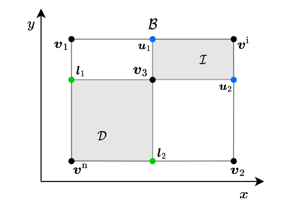
(a)

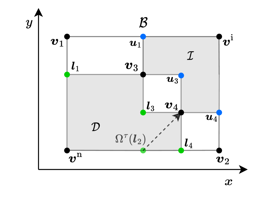
(b)

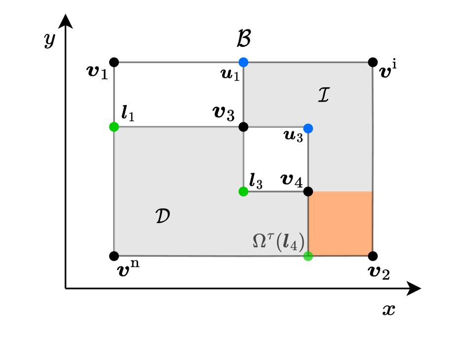
(c)

Figure 1: (a) The bounding box $\mathcal{B}$, delineated with solid lines, is defined by the nadir ${\bm{v}}^{\text{n}}$ and ideal ${\bm{v}}^{\text{i}}$ and contains all Pareto optimal solutions. The dominated set ${\mathcal{D}}$ and infeasible set ${\mathcal{I}}$ are defined by the current approximation to the Pareto front ${\mathcal{V}}=\{{\bm{v}}_{1},{\bm{v}}_{2},{\bm{v}}_{3}\}$ and are shaded. The lower bounds ${\bm{l}}\in{\mathcal{L}}$ are highlighted in green, while the upper bounds ${\bm{u}}\in{\mathcal{U}}$ are highlighted in blue. (b) After querying the Pareto oracle $\Omega^{\tau}$ with ${\bm{l}}_{2}$, ${\bm{v}}_{4}$ is added to the Pareto front and the set of lower bounds ${\mathcal{L}}$ and upper bounds ${\mathcal{U}}$ are updated to represent the new corners of ${\mathcal{D}}$ and ${\mathcal{I}}$ respectively. (c) When the Pareto oracle cannot find a feasible solution strictly dominating ${\bm{l}}_{4}$, it is added to the completed set ${\mathcal{C}}$ and the shaded orange area is added to the infeasible set ${\mathcal{I}}$.

Problem setup. We consider sequential multi-objective decision-making problems, modelled as a multi-objective Markov decision process (MOMDP). A MOMDP is a tuple $\bm{\mathcal{M}}=\langle\mathcal{S},\mathcal{A},\mathbf{P},\bm{\mathcal{R}},\allowbreak\mu,\gamma\rangle$ where $\mathcal{S}$ is the set of states, $\mathcal{A}$ the set of actions, $\mathbf{P}$ the transition function, $\bm{\mathcal{R}}:\mathcal{S}\times\mathcal{A}\times\mathcal{S}\to\mathbb{R}^{d}$ the vectorial reward function with $d\geq 2$ the number of objectives, $\mu$ the distribution over initial states and $\gamma$ the discount factor. In single-objective RL, it is common to learn a policy that maximises the expected return. In a MOMDP, however, there is generally not a single policy that maximises the expected return for all objectives (Hayes et al., 2022). As such, we introduce a partial ordering over policies on the basis of Pareto dominance and say that a policy $\pi\in\Pi$ Pareto dominates another if its expected return, defined as ${\bm{v}}^{\pi}:=\mathop{\mathbb{E}}_{\pi,\mu}\left[\sum_{t=0}^{\infty}\gamma^{t}\bm{\mathcal{R}}(s_{t},a_{t},s_{t+1})\right]$, Pareto dominates the expected return of the other policy.

Our goal is to learn a Pareto front of memory-based deterministic policies in MOMDPs. Such policies are relevant in safety-critical settings, where stochastic policies may have catastrophic outcomes but can Pareto dominate deterministic policies (Delgrange et al., 2020). Furthermore, for deterministic policies, it can be shown that memory-based policies may Pareto dominate stationary policies (Roijers & Whiteson, 2017). We define a deterministic memory-based policy as a Mealy machine $\pi=\langle\mathcal{Q},\pi_{a},\pi_{q},\mu_{q}\rangle$ where $\mathcal{Q}$ is a set of memory states, $\pi_{a}:\mathcal{S}\times\mathcal{Q}\to\mathcal{A}$ a deterministic next action function, $\pi_{q}:\mathcal{S}\times\mathcal{Q}\times\mathcal{A}\times\mathcal{S}\to\mathcal{Q}$ the memory update function and $\mu_{q}$ the initial memory state. In this setting, it is known that the Pareto front may be non-convex and thus cannot be fully recovered by methods based on linear scalarisation. Furthermore, to the best of our knowledge, no algorithm exists that produces a Pareto front for such policies in general MOMDPs.

4 Iterated Pareto Referent Optimisation

We present Iterated Pareto Referent Optimisation (IPRO) to learn a Pareto front in MOMDPs through a decomposition-based approach. We prove an upper bound on the maximum distance between the obtained solutions and the Pareto front and guarantee its convergence. While IPRO is introduced within the reinforcement learning context, it only requires a problem-specific method to solve the decomposed problem, indicating its potential for broader application. The execution of IPRO is illustrated in Figure 1.

4.1 Algorithm Overview

The core idea of IPRO is to bound the search space that may contain value vectors corresponding to Pareto optimal policies and iteratively remove sections from this space. This is achieved by leveraging an oracle to obtain a policy with its value vector in some target region and utilising this to update the boundaries of the search space. Detailed pseudocode is given in Algorithm 1.

Bounding the search space. It is first necessary to bound the space in which Pareto non-dominated solutions may exist. By definition, the box spanned by the nadir ${\bm{v}}^{\text{n}}$ and ideal ${\bm{v}}^{\text{i}}$ contains all such points (shown as $\mathcal{B}$ in Figure 1). Obtaining the ideal is done by maximising each objective independently, effectively reducing the MOMDP to a regular MDP that can be solved with conventional methods. The solutions constituting the ideal are further used to instantiate the Pareto front ${\mathcal{V}}$. Since obtaining the nadir is generally more complicated (Miettinen, 1998), we compute a lower bound of the nadir by minimising each objective independently, analogous to the instantiation of the ideal.

Obtaining a Pareto optimal policy. Given a bounding box, IPRO proceeds by identifying individual Pareto optimal policies. For this, we employ a Pareto oracle which can be considered as a solver for a particular constrained optimisation problem. Informally, a Pareto oracle $\Omega^{\tau}$ with tolerance $\tau$ takes as input a referent ${\bm{r}}$ and attempts to return a weakly Pareto optimal policy $\pi$ whose expected return ${\bm{v}}^{\pi}$ strictly dominates the referent. Importantly, the oracle’s output effectively guides IPRO in deciding which points may still correspond to Pareto optimal policies. When the oracle evaluation was successful, it is guaranteed that ${\bm{v}}^{\pi}$ is at least weakly Pareto optimal and therefore all points dominated by ${\bm{v}}^{\pi}$ do not correspond to Pareto optimal policies. Moreover, all points strictly dominating ${\bm{v}}^{\pi}$ are guaranteed to be infeasible, as otherwise $\pi$ would not have been returned as a weakly Pareto optimal policy. When the evaluation was unsuccessful, all points strictly dominating ${\bm{r}}$ may be excluded as they are guaranteed to be infeasible or within the tolerance $\tau$. We refer to Section 5 for a rigorous definition and theoretical results for Pareto oracles.

Reducing the search space. In the main loop of IPRO, we use the Pareto oracle to obtain new Pareto optimal solutions and exclude additional sections of search space. For this, we maintain a dominated set ${\mathcal{D}}$ and infeasible set ${\mathcal{I}}$, that respectively contain points dominated by the current Pareto front and points guaranteed infeasible by a previous oracle evaluation (Figure 1(a)). A naive approach would be to iteratively query the oracle, and adjust ${\mathcal{D}}$ and ${\mathcal{I}}$ until they cover the entire bounding box. However, in scenarios where Pareto oracle evaluations are expensive, such as when learning policies in a MOMDP, a more systematic approach is preferable to minimise the number of oracle evaluations.

We propose instead to select referents from a set of guaranteed lower bounds to ensure maximal improvement in each iteration. Intuitively, any remaining Pareto optimal solution ${\bm{v}}^{\ast}$ must strictly dominate some point on the boundary of the dominated set ${\mathcal{D}}$. Furthermore, ${\bm{v}}^{\ast}$ is necessarily upper bounded by some point on the boundary of the infeasible set ${\mathcal{I}}$. This insight allows us to define the lower bounds ${\mathcal{L}}$ and upper bounds ${\mathcal{U}}$, covering the inner corners of the dominated and infeasible sets respectively (Figure 1(a)). For the lower bounds, this ensures that ${\bm{v}}^{\ast}$ must strictly dominate at least one ${\bm{l}}\in{\mathcal{L}}$, further implying that ${\bm{v}}^{\ast}$ can be found by a Pareto oracle. Using some heuristic, IPRO selects a lower bound from ${\mathcal{L}}$ and presents this to the oracle. If the oracle evaluation is successful, a new solution is added to the Pareto front (Figure 1(b)). If the evaluation is unsuccessful, the lower bound itself is added to the set of completed points ${\mathcal{C}}$ (Figure 1(c)). This procedure is repeated until the distance for every upper bound to its closest lower bound falls below a user-provided tolerance threshold $\tau$, at which point it is guaranteed that a $\tau$-Pareto front is obtained.

While in Figure 1 all unexplored sections are contained in isolated rectangles, this is a special property of bi-objective problems. We propose a simplified variant of IPRO for such problems in Section 4.4. For more than two objectives, this property does not hold and necessitates careful updates of the lower and upper bounds and potentially costly referent selection. We refer to Appendix A for an extended discussion and pseudocode for updating the lower bounds.

Algorithm 1 The IPRO algorithm.

0:  A Pareto oracle $\Omega^{\tau}$ with tolerance $\tau$

0:  A $\tau$-Pareto front ${\mathcal{V}}$

1:  Get maximal points $\{{\bm{v}}^{1},\dotsc,{\bm{v}}^{d}\}$ to create the ideal ${\bm{v}}^{\text{i}}$

2:  Get minimal points to estimate the nadir ${\bm{v}}^{\text{n}}$

3:  Form a bounding box $\mathcal{B}$ from ${\bm{v}}^{\text{n}}$ and ${\bm{v}}^{\text{i}}$

4:  ${\mathcal{U}}\leftarrow\{{\bm{v}}^{\text{i}}\}$

5:  ${\mathcal{L}}\leftarrow\{{\bm{v}}^{\text{n}}\}$

6:  ${\mathcal{V}}\leftarrow\{{\bm{v}}^{1},\dotsc,{\bm{v}}^{d}\}$ and ${\mathcal{C}}\leftarrow\emptyset$

7:  for ${\bm{v}}\in\{{\bm{v}}^{1},\dotsc,{\bm{v}}^{d}\}$ do

8:     Update ${\mathcal{L}}$ using ${\bm{v}}$ (see Appendix A, Algorithm 2)

9:  end for

10:  while $\max_{{\bm{u}}\in{\mathcal{U}}}\min_{{\bm{v}}^{\prime}\in{\mathcal{V}}}\|{\bm{u}}-{\bm{v}}^{\prime}\|_{\infty}>\tau$ do

11:     ${\bm{l}}\leftarrow\textsc{Select}({\mathcal{L}})$

12:     $\textsc{success},{\bm{v}}^{\ast}\leftarrow\Omega^{\tau}({\bm{l}})$

13:     if success then

14:        ${\mathcal{V}}\leftarrow{\mathcal{V}}\cup\{{\bm{v}}^{\ast}\}$

15:     else

16:        ${\mathcal{C}}\leftarrow{\mathcal{C}}\cup\{{\bm{l}}\}$

17:     end if

18:     Update ${\mathcal{L}}$ and ${\mathcal{U}}$ (see Appendix A, Algorithm 2)

19:  end while

4.2 Upper Bounding the Error

Since ${\mathcal{U}}$ contains an upper bound for all remaining feasible solutions, we can use it to bound the distance between the current approximation of the Pareto front ${\mathcal{V}}_{t}$ and the remaining Pareto optimal solutions $\mathcal{V}^{\ast}\setminus{\mathcal{V}}_{t}$. Let the true approximation error $\varepsilon^{\ast}_{t}$ from ${\mathcal{V}}_{t}$ to the true Pareto front ${\mathcal{V}}^{\ast}$ at timestep $t$ be defined as $\sup_{{\bm{v}}^{\ast}\in\mathcal{V}^{\ast}\setminus{\mathcal{V}}_{t}}\min_{{\bm{v}}\in{\mathcal{V}}_{t}}\|{\bm{v}}^{\ast}-{\bm{v}}\|_{\infty}$. As ${\mathcal{U}}$ is finite for any $t<\infty$ by construction, we can substitute the $\sup_{{\bm{v}}^{\ast}\in\mathcal{V}^{\ast}\setminus{\mathcal{V}}_{t}}$ by a $\max_{{\bm{u}}\in{\mathcal{U}}}$, resulting in an upper bound on the true approximation error $\varepsilon^{\ast}_{t}$. We formalise this in Theorem 4.1 and provide a proof in Section B.4.

Theorem 4.1.

Let ${\mathcal{V}}^{\ast}$ be the true Pareto front, ${\mathcal{V}}_{t}$ the approximate Pareto front obtained by IPRO and $\varepsilon^{\ast}_{t}$ the true approximation error at timestep $t$. Then the following inequality holds,

$$\varepsilon^{\ast}_{t}\leq\max_{{\bm{u}}\in{\mathcal{U}}_{t}}\min_{{\bm{v}}\in{\mathcal{V}}_{t}}\|{\bm{u}}-{\bm{v}}\|_{\infty}.$$ (1)

One can verify this result in Figure 1(b) where ${\mathcal{U}}=\{{\bm{u}}_{1},{\bm{u}}_{3},{\bm{u}}_{4}\}$ contains the upper bounds on the remaining Pareto optimal solutions. Note that while approximate Pareto fronts are commonly computed with regard to the $L^{\infty}$ norm, this guarantee can be extended more generally to other distance metrics.

4.3 Convergence to a Pareto Front

As IPRO progresses, the sequence of errors generated by Theorem 4.1 can be shown to be monotonically decreasing and converges to zero. Intuitively, this can be observed in Figure 1(b) where the retrieval of a new Pareto optimal point reduces the distance to the upper bounds. Additionally, the closure of a section, illustrated in Figure 1(c), results in the removal of the upper point which subsequently reduces the remaining search space. Since IPRO terminates when the true approximation error is guaranteed to be at most equal to the tolerance $\tau$, this results in a $\tau$-Pareto front.

Theorem 4.2.

Given a Pareto oracle $\Omega^{\tau}$ and tolerance $\tau>0$, IPRO converges to a $\tau$-Pareto front in a finite number of iterations. For a Pareto oracle $\Omega^{\tau}$ with tolerance $\tau=0$, IPRO converges to the exact Pareto front as $t\to\infty$.

We provide a proof of Theorem 4.2 in Section B.5 with a mild assumption on the Pareto oracle that ensures sufficient progress in each iteration.

4.4 IPRO-2D: A Version for Bi-Objective Problems

While IPRO is applicable to problems with $d\geq 2$ objectives, updating the lower and upper bounds as well as selecting a new referent may be costly. We introduce a dedicated variant for bi-objective problems ($d=2$), IPRO-2D, where substantial simplifications are possible.

As shown in Figure 1, all remaining sections within the bounding box manifest as isolated rectangles, with each lower and upper bound precisely defining one such rectangle. When a new Pareto optimal solution is found, updating ${\mathcal{L}}$ and ${\mathcal{U}}$ can be done by adding at most two new points for both sets, each on one side of the adjusted boundary. Moreover, calculating the area of each rectangle is straightforward, making it possible to construct a priority queue that prioritises the processing of larger rectangles to ensure a rapid decrease in the upper bound of the error. The maximum error can be computed by taking the rectangle with the maximum distance between its lower and upper bound, rather than performing the full max-min operation in Equation 1.

5 Pareto Oracle

Obtaining a solution in a designated region is central to the design of IPRO. We introduce Pareto oracles for this purpose and derive theoretically sound methods that lead to effective implementations in practice.

5.1 Formalisation

In each iteration, IPRO queries a Pareto oracle with a referent selected from the set of lower bounds to identify a new weakly Pareto optimal policy in the target region. We define two variants of a Pareto oracle that differ in the quality of the returned policy as well as their adherence to the target region. First, when a tolerance of zero is required, we define weak Pareto oracles that return weakly Pareto optimal solutions. Importantly, since the points in ${\mathcal{L}}$ are inherently dominated by known points on the Pareto front, naively presenting them to a Pareto oracle may result in obtaining the same solution repeatedly without obtaining new solutions. We therefore require that the obtained solution strictly dominates the referent to guarantee that progress is made in each iteration.

Definition 5.1.

A weak Pareto oracle $\Omega^{\tau}$ with tolerance $\tau=0$ maps a referent ${\bm{r}}\in\mathbb{R}^{d}$ to a weakly Pareto optimal policy $\pi\in\Pi$ such that ${\bm{v}}^{\pi}>{\bm{r}}$ or returns False when no such policy exists.

While Definition 5.1 does not require any tolerance, the restriction to weakly Pareto optimal solutions may be limiting in practice. To overcome this, we define approximate Pareto oracles that are guaranteed to return Pareto optimal solutions but require a strictly positive tolerance. This ensures that sufficient progress is made in each iteration, as either a new Pareto optimal solution is found which is at least some minimal improvement over the lower bound or the entire section can be closed. Moreover, since such oracles return Pareto optimal solutions rather than only weakly optimal solutions, fewer evaluations of the oracle are necessary overall.

Definition 5.2.

An approximate Pareto oracle $\Omega^{\tau}$ with intrinsic tolerance $\bar{\tau}\geq 0$ and user-provided tolerance $\tau>\bar{\tau}$ maps a referent ${\bm{r}}\in\mathbb{R}^{d}$ to a Pareto optimal policy $\pi\in\Pi$ such that ${\bm{v}}^{\pi}\succeq{\bm{r}}+(\tau-\bar{\tau})$ or returns False when no policy $\pi$ exists such that ${\bm{v}}^{\pi}\succeq{\bm{r}}+\tau$.

We emphasise that, unlike weak Pareto oracles, approximate Pareto oracles contain an intrinsic tolerance $\bar{\tau}$ in addition to a user-provided tolerance $\tau$. Intuitively, the intrinsic tolerance specifies the minimal adjustment necessary for the oracle to only return solutions in the target region. The user-provided tolerance is in turn assumed to be strictly greater and their difference represents the minimal improvement that is acceptable to the user to warrant further consideration of the region. For some implementations of approximate Pareto oracles, the inherent tolerance is zero, avoiding the need to compute $\bar{\tau}$ and implying that the user is free to select any tolerance (see Section C.2).

To illustrate the difference between a weak and approximate Pareto oracle, we show a possible evaluation of both oracles with a given referent in Figure 2. We note that related concepts have been studied in multi-objective optimisation (Papadimitriou & Yannakakis, 2000) as well as multi-objective planning (Chatterjee et al., 2006).

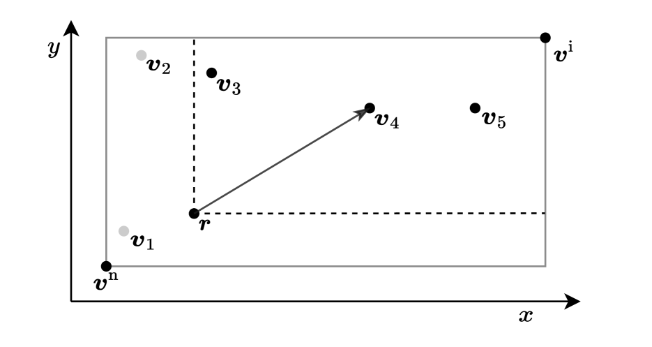
(a) A weak Pareto oracle.

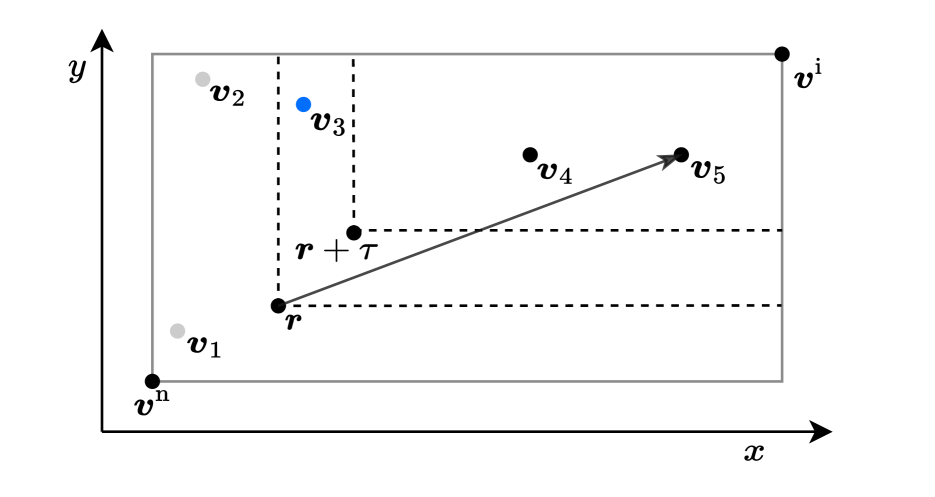
(b) An approximate Pareto oracle.

Figure 2: An illustration of both variants of a Pareto oracle. Solutions inside the target region are black, while solutions outside the target region are grey. (a) The weak Pareto oracle returns ${\bm{v}}_{4}$, which is in the target region but is only weakly Pareto optimal as it is dominated by ${\bm{v}}_{5}$. (b) The approximate Pareto oracle returns a Pareto optimal solution ${\bm{v}}_{5}$, but may fail to find ${\bm{v}}_{3}$, shown in blue.

5.2 Relation to Achievement Scalarising Functions

In Section 3, we introduced order representing and order approximating achievement scalarising functions (ASFs), highlighting their role in obtaining (weakly) Pareto optimal solutions. We now establish a direct application of these ASFs in constructing Pareto oracles. We refer to Appendix C for rigorous proofs of our theoretical results.

We first demonstrate that evaluating a weak Pareto oracle $\Omega^{\tau}$ with referent ${\bm{r}}$ can be framed as optimising an order representing ASF over a set of allowed policies $\Pi$. Since such ASFs guarantee that their maximum is reached within the target region at some weakly optimal solution, Theorem 5.3 follows immediately.

Theorem 5.3.

Let $s_{\bm{r}}$ be an order representing ASF. Then $\Omega^{\tau}({\bm{r}})=\operatorname*{arg\,max}_{\pi\in\Pi}s_{\bm{r}}({\bm{v}}^{\pi})$ with tolerance $\tau=0$ is a valid weak Pareto oracle.

This ensures that weakly optimal solutions can be obtained by proposing referents to an order representing ASF. However, practical considerations may lead us to favour an order approximating ASF, which yields Pareto optimal solutions instead. We demonstrate in Theorem 5.4 that such ASFs can indeed be applied to construct approximate Pareto oracles.

Theorem 5.4.

Let $s_{\bm{r}}$ be an order approximating ASF and let ${\bm{l}}\in\mathbb{R}^{d}$ be a lower bound such that only referents ${\bm{r}}$ are selected when ${\bm{r}}\succeq{\bm{l}}$. Then $s_{\bm{r}}$ has an inherent oracle tolerance $\bar{\tau}>0$ and for any user-provided tolerance $\tau>\bar{\tau}$, $\Omega^{\tau}({\bm{r}})=\operatorname*{arg\,max}_{\pi\in\Pi}s_{{\bm{r}}+\tau}({\bm{v}}^{\pi})$ is a valid approximate Pareto oracle.

From the definition of an order approximating ASF, we know that its maximum is reached at a Pareto optimal solution. However, since such ASFs may obtain this maximum outside the target region, it is necessary to shift the referent upwards by at least an inherent tolerance $\bar{\tau}$. This tolerance is dependent on an approximation parameter in the ASF, which governs the inclusion of additional points. Since it may be challenging to determine $\bar{\tau}$, a practical alternative is to utilise an order approximating ASF while still optimising $\operatorname*{arg\,max}_{{\bm{v}}^{\pi}\in\Pi}s_{\bm{r}}({\bm{v}}^{\pi})$, as is the case in the weak Pareto oracle. We empirically demonstrate in Section 7 that this strategy is effective in learning a Pareto front.

5.3 Principled Implementations

While Theorems 5.3 and 5.4 establish that an oracle may be implemented using an ASF, optimising the ASF over a given policy class may still be prohibitively expensive. Here, we show that efficient implementations can be derived from existing literature. First, the proposed approach using ASFs can be implemented by solving an auxiliary convex Markov decision process. In such models, the goal is to minimise a convex function, or equivalently maximise a concave function, over a set of admissible stationary distributions (Zahavy et al., 2021). Importantly, recent work has proposed multiple methods that come with strong convergence guarantees to solve convex MDPs (Zhang et al., 2020; Zahavy et al., 2021; Geist et al., 2022).

Corollary 5.5.

Let $s_{\bm{r}}$ be an ASF that is concave for any ${\bm{r}}\in\mathbb{R}^{d}$. Then, for any ${\bm{r}}\in\mathbb{R}^{d}$ and tolerance $\tau\geq 0$, a valid weak or approximate Pareto oracle $\Omega^{\tau}$ can be implemented for the class of stochastic policies by solving an auxiliary convex MDP.

In addition, approximate Pareto oracles can be implemented without optimising an ASF but rather by solving an auxiliary constrained Markov decision process. In a constrained MDP, an agent maximises a single reward function, but needs to adhere to additional constraints. Intuitively, a Pareto oracle can then be constructed by optimising the sum of rewards, while staying in the target region with some positive tolerance.

Corollary 5.6.

For any referent ${\bm{r}}\in\mathbb{R}^{d}$, tolerance $\tau>0$ and policy class, a valid approximate Pareto oracle $\Omega^{\tau}$ can be implemented by solving an auxiliary constrained MDP.

When the constrained MDP is known and both state and action sets are finite, computing an optimal policy can be done in polynomial time (Altman, 1999). Additionally, several algorithms with theoretical foundations have been proposed for solving such models within a reinforcement learning context (Achiam et al., 2017; Ding et al., 2021). We provide an extended discussion of these results with related proofs in Section C.2.

6 Deterministic Memory-Based Policies

As shown in Sections 4 and 5, IPRO obtains the Pareto front for any policy class with a valid Pareto oracle. We now design a Pareto oracle for deterministic memory-based policies, which are particularly relevant in safety-critical scenarios or when prioritising explainability and interpretability.

6.1 ASF Selection

In our experimental evaluation, we utilise the well-known augmented Chebyshev scalarisation function (Nikulin et al., 2012), shown in Equation 2. We highlight that this ASF is concave for all referents, implying its applicability together with Corollary 5.5 for stochastic policies as well.

$$s_{\bm{r}}({\bm{v}})=\min_{j\in\{1,\dotsc,d\}}\lambda_{j}({\bm{v}}_{j}-{\bm{r}}_{j})+\rho\sum_{j=1}^{d}\lambda_{j}({\bm{v}}_{j}-{\bm{r}}_{j})$$ (2)

Here, $\bm{\lambda}>0$ serves as a normalisation constant for the different objectives, and $\rho$ is a parameter determining the strength of the augmentation term. Selecting $\bm{\lambda}=({\bm{v}}^{\text{i}}-{\bm{v}}^{\text{n}})^{-1}$ scales any vector ${\bm{v}}$ relative to the distance between the nadir ${\bm{v}}^{\text{n}}$ and ideal ${\bm{v}}^{\text{i}}$, thereby ensuring a balanced scale across all objectives. This normalisation prevents the dominance of one objective over another, a challenge that is otherwise difficult to overcome (Abdolmaleki et al., 2020).

Equation 2 serves as a weak or approximate Pareto oracle, depending on the augmentation parameter $\rho$. When $\rho=0$, the augmentation term is cancelled and the minimum ensures that only vectors in the target region have non-negative values. However, optimising a minimum may result in weakly Pareto optimal solutions (e.g. $(1,2)$ and $(1,1)$ share the same minimum). For $\rho>0$, the optimal solution will be Pareto optimal (the sum of $(1,2)$ is greater than that of $(1,1)$) but may exceed the target region.

6.2 Practical Implementation

It has been shown that verifying whether a memory-based deterministic feasible policy exists in a MOMDP which dominates a referent is NP-hard (Chatterjee et al., 2006). To overcome this challenge, we extend single-objective reinforcement learning algorithms to optimise the ASF in Equation 2. It is common in MORL to encode the memory of a policy by its accrued reward at timestep $t$ defined as ${\bm{v}}^{\text{acc}}_{t}=\sum_{k=0}^{t-1}\gamma^{k}\bm{\mathcal{R}}(s_{k},a_{k},s_{k+1})$. In our implementation, this accrued reward is added to the observation.

DQN. We extend the GGF-DQN algorithm, which optimises for the generalised Gini welfare of the expected returns (Siddique et al., 2020), to optimise any scalarisation function $f$. We note that GGF-DQN is itself an extension of DQN (Mnih et al., 2015). Concretely, we train a Q-network such that $\bm{Q}(s_{t},a_{t})={\bm{r}}+\gamma\bm{Q}(s_{t+1},a^{\ast})$ where the optimal action $a^{\ast}$ is computed using the accrued reward and scalarisation function $f$,

$$a^{\ast}=\operatorname*{arg\,max}_{a\in\mathcal{A}}f\left({\bm{v}}^{\text{acc}}_{t+1}+\gamma\bm{Q}\left(s_{t+1},a\right)\right).$$ (3)

Policy gradient. We modify policy gradient algorithms to optimise $J(\pi)=f({\bm{v}}^{\pi})$, where $f$ is a scalarisation function and $\pi$ a parameterised policy with parameters $\theta$. For differentiable $f$, the policy gradient becomes $\nabla_{\theta}J(\pi)=f^{\prime}({\bm{v}}^{\pi})\cdot\nabla_{\theta}{\bm{v}}^{\pi}(s_{0})$ (Reymond et al., 2023). This gradient update computes the regular single-objective gradient for all objectives and takes the dot product with the gradient of the scalarisation function with respect to the expected returns.

Rather than learning a policy with the vanilla policy gradient, we propose to use either the A2C (Mnih et al., 2016) or PPO (Schulman et al., 2017) update per objective instead. For A2C, we use generalised advantage estimation (Schulman et al., 2018) as a baseline, while for PPO we substitute the policy gradient with a clipped surrogate objective function. To ensure deterministic policies, we take actions according to $\operatorname*{arg\,max}_{a\in\mathcal{A}}\pi(a|s)$ during policy evaluation. Although this potentially changes the policy, effectively employing a policy that differs from the one initially learned, empirical observations suggest that these algorithms typically converge toward deterministic policies in practice.

Generalisation using an extended network. Rather than making separate calls to one of the previous reinforcement learning methods for each oracle evaluation, we employ extended networks (Abels et al., 2019) to improve sample efficiency. Concretely, we extend our actor and critic networks to take a referent as additional input, enabling their reuse across IPRO iterations. Furthermore, we introduce a pre-training routine that trains a policy on randomly sampled referents for a fixed number of episodes. To take full advantage of this pre-training, we perform additional off-policy updates for referents not used in data collection. While this does not impact DQN, the policy gradient algorithms expect the behaviour and target policy to be the same. For A2C, we resolve this using importance sampling and for PPO by implementing an off-policy variant (Meng et al., 2023).

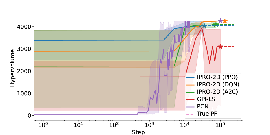
(a) Deep Sea Treasure

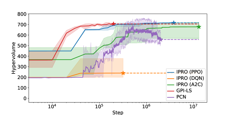
(b) Minecart

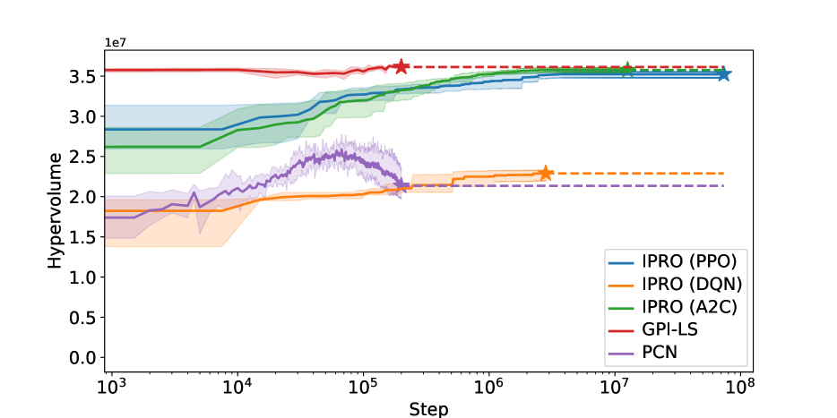
(c) MO-Reacher

Figure 3: The mean hypervolume with 95-percentile interval over time. Stars indicate when each algorithm finished and lines are extended to better compare final values. The pretraining phase of IPRO is not shown. We note that the x-axis is on a log scale.

7 Experiments

We evaluate IPRO(-2D) with the modified versions of DQN, A2C, and PPO proposed in Section 6 to optimise the augmented Chebyshev scalarisation function in Equation 2. Our code will be made publicly available upon acceptance.

Table 1: The minimum $\varepsilon$ shift necessary to obtain any undiscovered Pareto optimal solution. The best mean is in bold.

Env	Algorithm	$\varepsilon$
	IPRO (PPO)	$5.40\pm 2.58$
	IPRO (A2C)	$4.20\pm 1.83$
DST	IPRO (DQN)	$\bm{0.00\pm 0.00}$
	PCN	$\bm{0.00\pm 0.00}$
	GPI-LS	$32.60\pm 45.20$
	IPRO (PPO)	$0.66\pm 0.07$
	IPRO (A2C)	$0.54\pm 0.11$
Minecart	IPRO (DQN)	$1.14\pm 0.01$
	PCN	$0.67\pm 0.12$
	GPI-LS	$\bm{0.28\pm 0.09}$
	IPRO (PPO)	$5.45\pm 1.22$
	IPRO (A2C)	$\bm{2.65\pm 0.38}$
MO-Reacher	IPRO (DQN)	$14.78\pm 1.43$
	PCN	$18.24\pm 2.52$
	GPI-LS	$5.28\pm 0.56$

Setup. Since IPRO is the first general-purpose MORL method capable of learning a Pareto front of deterministic policies, we evaluate it against baselines that require additional domain knowledge. In particular, we select PCN (Reymond et al., 2022) which is specifically designed for deterministic environments and GPI-LS (Alegre et al., 2023) and Envelope Q-learning (EQL) (Yang et al., 2019) that both assume a convex Pareto front. We report the hypervolume over time, measuring the total volume dominated by Pareto optimal solutions relative to a reference point. Additionally, to measure the quality of the final Pareto fronts we compute the minimum $\varepsilon$ for each algorithm necessary to obtain any Pareto optimal value vector obtained by another algorithm. Note that EQL is omitted from Figure 3 and Table 1 since it was found to perform worse than GPI-LS across all environments. Experiments are repeated across five seeds with additional details presented in Appendix D.

Deep Sea Treasure $(d=2)$. Deep Sea Treasure (DST) is a deterministic environment where a submarine seeks treasure while minimising fuel consumption. DST has a Pareto front with solutions in concave regions (Vamplew et al., 2011), making it impossible for convex hull algorithms to recover all Pareto optimal solutions. When pairing IPRO-2D with any of the three Pareto oracles, the obtained hypervolume closely approximates the true Pareto front. Notably, the choice of reference point in DST disproportionately benefits the convex hull obtained by GPI-LS compared to obtaining a different subset of Pareto optimal solution. When comparing the approximation quality instead, IPRO learns qualitative approximations and in particular consistently learns the complete Pareto front when paired with DQN. The convex hull methods naturally have poorer approximations.

Minecart $(d=3)$. Minecart is a stochastic environment where the agent collects two ore types while minimising fuel consumption and has a convex Pareto front (Abels et al., 2019). We observe that IPRO with A2C achieves a greater hypervolume than all other methods and its approximation distance $\varepsilon$ is competitive to that obtained by GPI-LS. The DQN oracle struggles to learn a qualitative Pareto front in this environment. During evaluation, we noted a performance drop for GPI-LS without prioritised experience replay and hypothesise that incorporating this technique may enhance the DQN oracle’s performance here as well.

MO-Reacher $(d=4)$. MO-Reacher is a deterministic environment where four balls are arranged in a circle and the goal is to minimise the distance to each ball. Since it is both deterministic and has a mostly convex Pareto front it suits all baselines. Moreover, due to its high dimensionality, it is generally challenging for MORL algorithms. We find that IPRO obtains close to the optimal hypervolume and the best approximation to the Pareto front. Due to IPRO’s iterative mechanism, this does come at the price of increased sample complexity. We emphasise that GPI-LS employs iterative fine-tuning of policies, while IPRO constructs a new policy in each iteration. Adapting IPRO to include a similar mechanism is a promising direction for future work.

Discussion. These results demonstrate IPRO’s competitiveness to the baselines in all environments, an impressive feat given that all baselines perform significantly worse in one of the environments. Moreover, IPRO stands out without requiring domain knowledge for proper application, unlike its counterparts. Finally, in both Minecart and MO-Reacher, IPRO attains top performance in one of the metrics and learns a qualitative approximation to the Pareto front, showcasing its scalability beyond bi-objective problems.

8 Conclusion

We introduce IPRO to provably learn a Pareto front in MOMDPs. IPRO iteratively proposes referents to a Pareto oracle and uses the returned solution to trim sections from the search space. We formally define Pareto oracles and derive principled implementations. We show that IPRO converges to a Pareto front and comes with strong guarantees with respect to the approximation error. Our empirical analysis finds that IPRO learns high-quality Pareto fronts while requiring less domain knowledge than baselines. For future work, we plan to apply IPRO to problems beyond MORL and explore alternative Pareto oracle implementations.

Impact Statement

This paper presents work whose goal is to advance the field of multi-objective decision-making and in particular multi-objective reinforcement learning. Multi-objective reinforcement learning can be used to better inform decision-makers by informing them about the different alternatives. This can be empowering to individual users.

Appendix A Additional Discussion of IPRO

We offer a more in-depth analysis of our algorithm, Iterated Pareto Referent Optimisation (IPRO). This extended discussion includes additional pseudocode for IPRO and a breakdown of its implementation. Furthermore, we consider how to select referents from the set of lower bounds and examine alterations to the theoretical algorithm that improve IPRO’s practical performance when paired with imprecise Pareto oracles.

A.1 Implementation of IPRO

IPRO follows an inner-outer loop structure. As discussed in Section 4, IPRO tracks the current Pareto front and excluded sections and iteratively proposes referents to a Pareto oracle. We now consider these phases in more detail.

Tracking the dominated and infeasible set. Recall that all points in the dominated set ${\mathcal{D}}$ are Pareto dominated by a point in the current approximation to the Pareto front ${\mathcal{V}}$. Moreover, all points in the infeasible set ${\mathcal{I}}$ are guaranteed to be infeasible as determined by the Pareto oracle. Since these sets contain points excluded from further consideration, it is essential to track them. Instead of explicitly monitoring these sets, we maintain the points on the Pareto front ${\mathcal{V}}$ and the completed set ${\mathcal{C}}$. Through these sets, we can compute the hypervolume covered by ${\mathcal{D}}$ and ${\mathcal{I}}$, providing an estimate of the overall coverage achieved by IPRO.

Tracking the lower and upper bounds. An important concept in IPRO is the notion of lower and upper bounds. For the set of lower bounds ${\mathcal{L}}$, we demonstrate in Appendix C that every remaining Pareto optimal solution must strictly dominate at least one ${\bm{l}}\in{\mathcal{L}}$. Furthermore, for all remaining Pareto optimal solutions ${\bm{v}}^{\ast}$ the set of upper bounds ${\mathcal{U}}$ contains an upper bound ${\bm{u}}$ such that ${\bm{u}}\succeq{\bm{v}}^{\ast}$. Visually, as shown in Figure 1, the set of lower bounds contains the inner corners of the dominated set, while the set of upper bounds contains the inner corners of the infeasible set.

The lower and upper bounds play a crucial role in deriving both our convergence guarantee and runtime guarantee on the largest distance to remaining Pareto optimal solutions. Consequently, tracking these sets is of paramount importance. When initialising the bounding box $\mathcal{B}$, the only lower bound is the nadir ${\bm{v}}^{\text{n}}$ and the only upper bound is the ideal ${\bm{v}}^{\text{i}}$. Upon introducing a new point ${\bm{v}}^{\ast}$ to the Pareto front, we examine the lower set to identify points that have become strictly dominated by it. If ${\bm{l}}$ is such a dominated point, it is replicated $d$ times, each time adjusting one dimension of the vector to align with the boundary of the newly added point ${\bm{v}}^{\ast}$. Since this approach may generate points within the dominated set ${\mathcal{D}}$, we perform a pruning step to eliminate points not on the boundary. Pseudocode for updating the lower bounds is provided in Algorithm 2 and updating the upper bounds is analogous.

Algorithm 2 Computing the lower set.

0:  A bounding box $\mathcal{B}$, previous lower set ${\mathcal{L}}_{t-1}$ and Pareto optimal solution ${\bm{v}}^{\ast}$

0:  The updated lower set ${\mathcal{L}}_{t}$

1:  ${\mathcal{L}}_{t}\leftarrow\{\}$

2:  for ${\bm{l}}\in{\mathcal{L}}_{t-1}$ do

3:     if ${\bm{v}}^{\ast}>{\bm{l}}$ then

4:        for $j\in[d]$ do

5:           ${\bm{l}}^{\prime}\leftarrow{\bm{l}}$

6:           ${\bm{l}}^{\prime}_{j}\leftarrow{\bm{v}}^{\ast}_{j}$

7:           ${\mathcal{L}}_{t}\leftarrow{\mathcal{L}}_{t}\cup\{{\bm{l}}^{\prime}\}$

8:        end for

9:     else

10:        ${\mathcal{L}}_{t}\leftarrow{\mathcal{L}}_{t}\cup\{{\bm{l}}\}$

11:     end if

12:  end for

13:  ${\mathcal{L}}_{t}\leftarrow\textsc{Prune}({\mathcal{L}}_{t})$

Postprocessing. While IPRO inherently requires no postprocessing, there exists a possibility that weakly Pareto optimal points added during IPRO’s execution have become dominated by subsequent additions to the Pareto front. While this does not impact the hypervolume of the final Pareto front, it could pose a challenge for decision-makers in selecting their preferred solution. To streamline the set presented to decision-makers, we enhance the obtained Pareto front by eliminating dominated points. In our implementation, we further include in the approximate Pareto front all solutions rejected by IPRO before the pruning step. While these solutions should in theory never be Pareto optimal, this step may, in practice, reveal additional Pareto optimal solutions.

A.2 Referent Selection

The iterative process constructed in IPRO involves proposing referents to a Pareto oracle. Naturally, a crucial question arises: how should these referents be chosen? While our theoretical outcomes are not contingent on a particular method for selecting referents, we propose the use of the hypervolume improvement heuristic. This heuristic suggests referents that, when incorporated into the infeasible set, would yield the greatest increase in hypervolume. Intuitively, referents with a high hypervolume improvement indicate a large unexplored region that dominates it, suggesting that new Pareto optimal solutions may be found there. We define this formally in Definition A.1

Definition A.1 (Hypervolume Improvement).

Let ${\bm{r}}\in\mathbb{R}^{d}$ be a reference point and $HV(S,{\bm{r}})$ be the hypervolume of a set $S$ with respect to the reference point. The hypervolume improvement $HVI$ of a point ${\bm{v}}\in\mathbb{R}^{d}$ is defined as the contribution of ${\bm{v}}$ to the hypervolume when added to $S$, i.e. $HVI({\bm{v}},S,{\bm{r}})=HV\left(S\cup\{{\bm{v}}\},{\bm{r}}\right)-HV(S,{\bm{r}})$.

It is worth noting that computing the hypervolume improvement for a large number of points can become prohibitively expensive, as it necessitates a new hypervolume computation for each point. This computational cost is one of the main reasons why the dedicated 2D variant of IPRO is more efficient. Concretely, in the two-dimensional case, all remaining area is made up of isolated rectangles described by one lower and upper bound. For these rectangles, we can efficiently compute the area and keep a priority queue of rectangles based on the $L^{\infty}$ distance between their lower and upper bound. Selecting the next referent can be done by taking the first rectangle from the priority queue and using its lower bound as the referent.

Finally, we highlight that depending on prior knowledge regarding the Pareto front’s shape or specific regions of interest, the referent selection method can be readily adapted and alternative metrics for assessing improvement could be incorporated into the process.

A.3 Improving Robustness

We extend IPRO to accommodate imperfect Pareto oracles by integrating a backtracking procedure. This procedure is triggered whenever a solution is returned that violates a decision made in a previous iteration. To implement this robustness feature, we maintain a sequence denoted as $\left\{\left({\bm{l}}_{t},{\bm{v}}_{t}\right)\right\}_{t\in\mathbb{N}}$ where each pair records the lower bound and retrieved solution for a given iteration. When, at time step $n$, the returned solution ${\bm{v}}_{n}$ strictly dominates a point ${\bm{c}}\in{\mathcal{C}}_{n}$ or ${\bm{v}}^{\ast}\in{\mathcal{V}}_{n}$, it indicates an incorrect oracle evaluation in a previous iteration. To address this issue, we initiate a replay of the sequence of pairs. Let $\bar{t}$ denote the time step at which the incorrect result was initially returned. For the subsequence $\left\{\left({\bm{l}}_{t},{\bm{v}}_{t}\right)\right\}_{0\leq t<\bar{t}}$, we replay the pairs using the standard IPRO updates and consider ${\bm{v}}_{n}$ as the retrieved solution for ${\bm{l}}_{\bar{t}}$.

For the subsequence $\left\{\left({\bm{l}}_{t},{\bm{v}}_{t}\right)\right\}_{\bar{t}<t<n}$, we apply different conditions than in the original iterations and leverage the transitivity property of Pareto dominance to recycle the pairs. Specifically, for every $({\bm{v}}_{t},{\bm{l}}_{t})$ we verify whether the evaluation was successful, in which case it is guaranteed that ${\bm{v}}_{t}$ was weakly Pareto optimal. When another lower bound ${\bm{l}}^{\prime}$ exists in the corrected set of lower bounds, ${\bm{v}}_{t}$ can be returned as the solution for ${\bm{l}}^{\prime}$ and is added using the standard IPRO update rule. When the original evaluation was not successful, ${\bm{l}}_{t}$ was added to the completed set and any point dominating it was guaranteed to be infeasible. Therefore, if a new lower bound ${\bm{l}}^{\prime}$ exists such that ${\bm{l}}^{\prime}\succeq{\bm{l}}_{t}$, ${\bm{l}}^{\prime}$ can be added to the corrected completed set as well.

Appendix B Theoretical Results for IPRO

In this section, we provide the omitted proofs for IPRO from Section 4. These results establish both the upper bound on the true approximation error as well as convergence guarantees to the true Pareto front in the limit or to an approximate Pareto front in a finite number of iterations.

B.1 Definitions

Before presenting the proofs for IPRO, it is necessary to define the sets that are tracked in IPRO. Let $\mathcal{B}=\prod_{j=1}^{d}[{\bm{v}}^{\text{n}}_{j},{\bm{v}}^{\text{i}}_{j}]$ be the bounding box defined by a strict lower bound of the true nadir ${\bm{v}}^{\text{n}}$ and the ideal ${\bm{v}}^{\text{i}}$. The set ${\mathcal{V}}_{t}$ contains the obtained Pareto front at timestep $t$ while the completed set ${\mathcal{C}}_{t}$ contains the referents for which the Pareto oracle evaluation was unsuccessful. We then define the dominated set ${\mathcal{D}}$ and infeasible set ${\mathcal{I}}$ as follows.

Definition B.1.

The dominated set ${\mathcal{D}}_{t}$ at timestep $t$ contains all points in the bounding box that are dominated by or equal to a point in the current Pareto front, i.e. ${\mathcal{D}}_{t}=\left\{{\bm{v}}\in\mathcal{B}\mid\exists{\bm{v}}^{\prime}\in{\mathcal{V}}_{t},{\bm{v}}^{\prime}\succeq{\bm{v}}\right\}$.

Definition B.2.

The infeasible set ${\mathcal{I}}_{t}$ at timestep $t$ contains all points in the bounding box that dominate or are equal to a point in the union of the current Pareto front and completed referents, i.e. ${\mathcal{I}}_{t}=\left\{{\bm{v}}\in B\mid\exists{\bm{v}}^{\prime}\in{\mathcal{V}}_{t}\cup C_{t},{\bm{v}}\succeq{\bm{v}}^{\prime}\right\}$.

Note that in the definition of the infeasible set, we consider not only those points dominated by the current Pareto front but also the points dominated by the referents that failed to result in new solutions.

During the execution of IPRO, it is necessary to recognise the remaining unexplored sections. For this, we define the boundaries, interiors and reachable boundaries of the dominated and infeasible set. Let $\overline{S}$ be the closure of a subset $S$ in some topological space and $\partial S$ be its boundary. By a slight abuse of notation, we say that $\partial{\mathcal{D}}_{t}=\overline{(\mathcal{B}\setminus{\mathcal{D}}_{t})}\cap\overline{{\mathcal{D}}_{t}}$ is the boundary of ${\mathcal{D}}_{t}$ in $\mathcal{B}$ and $\text{int }{\mathcal{D}}_{t}={\mathcal{D}}_{t}\setminus\partial{\mathcal{D}}_{t}$ is the interior of ${\mathcal{D}}_{t}$ in $\mathcal{B}$. We define the boundary and interior of the infeasible set analogously. Finally, we define the reachable boundaries of these sets which together delineate the remaining available search space and illustrate all defined subsets in Figure 4 for the two-dimensional case.

Definition B.3.

The reachable boundary of ${\mathcal{D}}_{t}$, denoted $\partial^{r}{\mathcal{D}}_{t}$ at timestep $t$ is defined as $\partial^{r}{\mathcal{D}}_{t}=\partial{\mathcal{D}}_{t}\setminus{\mathcal{I}}_{t}$.

Definition B.4.

The reachable boundary of ${\mathcal{I}}_{t}$, denoted $\partial^{r}{\mathcal{I}}_{t}$ at timestep $t$ is defined as $\partial^{r}{\mathcal{I}}_{t}=\partial{\mathcal{I}}_{t}\setminus{\mathcal{D}}_{t}$.

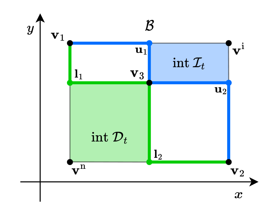
(a)

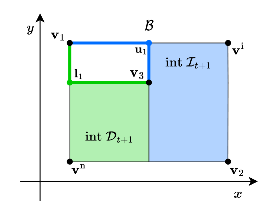
(b)

Figure 4: (a) The reachable boundaries of ${\mathcal{D}}_{t}$ (green) and ${\mathcal{I}}_{t}$ (blue) indicated with solid lines and their interiors (shaded) when no section is completed. (b) When completing the section at ${\bm{l}}_{2}$, parts of the reachable boundary at timestep $t$ become unreachable at timestep $t+1$.

For the reachable boundaries of the dominated and infeasible sets, we define two important subsets containing the respective lower and upper bounds of the remaining solutions on the Pareto front. The set of lower bounds ${\mathcal{L}}$ contains the points on the reachable boundary of the dominated set such that no other point on the reachable boundary exists which is dominated by it. Similarly, the set of upper bounds ${\mathcal{U}}$ contains the points on the reachable boundary of the infeasible set such that no other point exists on the reachable boundary that dominates it. Conceptually, these points are the inner corners of their respective boundary as observed in Figure 4.

Definition B.5 (Lower Bounds).

The set of lower bounds at timestep $t$ is defined as ${\mathcal{L}}_{t}=\left\{{\bm{l}}\in\partial^{r}{\mathcal{D}}_{t}\mid\nexists{\bm{v}}\in\partial^{r}{\mathcal{D}}_{t},{\bm{l}}\succ{\bm{v}}\right\}$.

Definition B.6 (Upper Bounds).

The set of upper bounds at timestep $t$ is defined as ${\mathcal{U}}_{t}=\left\{{\bm{u}}\in\partial^{r}{\mathcal{I}}_{t}\mid\nexists{\bm{v}}\in\partial^{r}{\mathcal{I}}_{t},{\bm{v}}\succ{\bm{u}}\right\}$.

B.2 Assumptions

We explicitly state and motivate the assumptions underpinning our theoretical results. We emphasise that all assumptions are either on an implementation level, efficiently verifiable or guaranteed to hold for significant domains of interest.

First, we assume that the problem is not trivial and there exist unexplored regions in the bounding box $\mathcal{B}$ after finding the first $d$ weakly Pareto optimal solutions. This assumption is not hindering, since after the initialisation phase we can run a pruning algorithm such as PPrune (Roijers & Whiteson, 2017), which takes as input a set of vectors and outputs only the Pareto optimal ones, and terminate IPRO if this is the case.

Assumption B.7.

For any MOMDP $\bm{\mathcal{M}}$ with $d$-dimensional reward function, we assume that for the initial Pareto front ${\mathcal{V}}_{0}=\{{\bm{v}}_{1},\dotsc,{\bm{v}}_{d}\}$ it is guaranteed that $|\textsc{PPrune}({\mathcal{V}}_{0})|>1$.

In addition, we provide assumptions necessary for weak Pareto oracles to ensure their convergence to the true Pareto front in the limit. Intuitively, we first assume that the referent selection mechanism is not antagonistic and we select in some iterations a referent that may reduce the error estimate. Note that this can be readily implemented using a randomised method which assigns a strictly positive probability to each lower bound in ${\mathcal{L}}$. Alternatively, we can explicitly construct the set of lower bounds that are expected to reduce the error and select from this set rather than the entire set of lower bounds.

Assumption B.8.

Let $\varepsilon_{t}=\max_{{\bm{u}}\in{\mathcal{U}}_{t}}\min_{{\bm{v}}\in{\mathcal{V}}_{t}}\|{\bm{u}}-{\bm{v}}\|_{\infty}$ be the upper bound on the true error $\varepsilon^{\ast}_{t}$ at timestep $t$. We define ${\mathcal{U}}^{\varepsilon}_{t}\subseteq{\mathcal{U}}_{t}$ to be the subset of upper bounds for which the error is equal to $\varepsilon_{t}$ and ${\mathcal{L}}^{\varepsilon}_{t}\subseteq{\mathcal{L}}_{t}$ to be the subset of lower bounds such that for all ${\bm{l}}\in{\mathcal{L}}^{\varepsilon}_{t}$ there is an ${\bm{u}}\in{\mathcal{U}}^{\varepsilon}_{t}:{\bm{u}}>{\bm{l}}$. As $t\to\infty$, an ${\bm{l}}\in{\mathcal{L}}^{\varepsilon}_{t}$ is almost surely selected as a referent.

The next assumption ensures that the oracle is not antagonistic and that it is capable of yielding any Pareto optimal solution. In other words, no solution is excluded by the Pareto oracle a priori. While this may be challenging to verify, in practice this can be satisfied by implementing a robust oracle.

Assumption B.9.

Let $\Omega^{\tau}$ be a weak Pareto oracle with tolerance $\tau=0$. For all undiscovered Pareto optimal solutions ${\bm{v}}^{\ast}\in\mathcal{V}^{\ast}\setminus{\mathcal{V}}_{t}$ there exists some lower bound ${\bm{l}}$ such that $\Omega^{\tau}({\bm{l}})={\bm{v}}^{\ast}$ and as $t\to\infty$, ${\bm{l}}$ is almost surely added to ${\mathcal{L}}_{t}$.

The final assumption that is necessary is on the shape of the Pareto front. Concretely, we assume that every segment of the Pareto front contains its endpoints. This is necessary to ensure that we may close all gaps between segments eventually, as otherwise we are never able to reduce the error estimate of IPRO below that of the largest gap. Importantly, B.10 holds when considering stochastic policies in finite MOMDPs, since the set of occupancy measures is a closed convex polytope (Altman, 1999).

Assumption B.10.

The Pareto front is the union of a finite number of paths (i.e. a continuous function $f:[0,1]\to\mathbb{R}^{d}$).

B.3 Supporting Lemmas

We provide supporting lemmas that formalise the contents of the sets defined in Section B.1 and their relation to the remaining feasible solutions. Concretely, we first demonstrate that the interior of the infeasible set contains only infeasible points or points within the acceptable tolerance, which is a consequence of having a strictly positive distance to the boundary. Combined with the dominated set, which inherently contains only dominated solutions, we can then significantly reduce the search space that is left to explore.

Lemma B.11.

Given an oracle $\Omega^{\tau}$ with tolerance $\tau$, then at all timesteps $t$ and for all ${\bm{i}}\in{\mathcal{I}}_{t}$, ${\bm{i}}$ is infeasible or within the tolerance $\tau$ of a point on the current estimate of the Pareto front ${\mathcal{V}}_{t}$.

Proof.

Recall that the interior of the infeasible set is defined as follows,

$$\text{int }{\mathcal{I}}_{t}={\mathcal{I}}_{t}\setminus\partial{\mathcal{I}}_{t}.$$ (4)

Let ${\bm{v}}\in\text{int }{\mathcal{I}}_{t}$ be a point in the interior of the infeasible set. Then there exists an open ball centred around ${\bm{v}}$ with a strictly positive radius $r$ such that $B_{r}({\bm{v}})\subseteq\text{int }{\mathcal{I}}_{t}$. Let ${\bm{v}}^{\prime}\in B_{r}({\bm{v}})$ be a point in the ball such that ${\bm{v}}>{\bm{v}}^{\prime}$ which can be obtained by taking ${\bm{v}}$ and subtracting a value $\delta\in(0,r)$. Since ${\bm{v}}^{\prime}\in\text{int }{\mathcal{I}}_{t}$, the definition of the infeasible set (Definition B.2) ensures that there exists a point $\bar{{\bm{v}}}\in{\mathcal{V}}_{t}\cup C_{t}$ such that ${\bm{v}}^{\prime}\succeq\bar{{\bm{v}}}$. By the transitivity of Pareto dominance, we then have that ${\bm{v}}>\bar{{\bm{v}}}$.

Let us now consider the two cases for $\bar{{\bm{v}}}$. Assume first that $\bar{{\bm{v}}}\in{\mathcal{V}}_{t}$. If ${\bm{v}}$ is a feasible solution and knowing that ${\bm{v}}>\bar{{\bm{v}}}$ implies that $\bar{{\bm{v}}}$ is not weakly Pareto optimal. Therefore, $\bar{{\bm{v}}}$ would not have been returned by a weak or approximate Pareto oracle. As such, ${\bm{v}}$ must be infeasible.

When $\bar{{\bm{v}}}\in C_{t}$ it was added after the oracle evaluation at $\bar{\bm{v}}$ was unsuccessful. For a weak Pareto oracle $\Omega^{\tau}$ with tolerance $\tau=0$, this again guarantees that ${\bm{v}}$ is infeasible since ${\bm{v}}>\bar{\bm{v}}$. For an approximate Pareto oracle $\Omega^{\tau}$ with tolerance $\tau>0$, we distinguish between two cases. If ${\bm{v}}\succeq\bar{\bm{v}}+\tau$, ${\bm{v}}$ is infeasible since $\Omega^{\tau}$ would otherwise have returned it. Finally, by the construction of the set of lower bounds ${\mathcal{L}}$, there must exist a point ${\bm{v}}^{\ast}$ on the current Pareto front ${\mathcal{V}}_{t}$ such that ${\bm{v}}^{\ast}+\tau\succeq{\bm{v}}$ and therefore ${\bm{v}}$ was within the tolerance. ∎

Given the result for the infeasible solutions, we now focus instead on the remaining feasible solutions. Here, we demonstrate that all feasible solutions are strictly lower bounded by ${\mathcal{L}}$ and upper bounded by ${\mathcal{U}}$.

Lemma B.12.

At any timestep $t$, the set of lower bounds ${\mathcal{L}}_{t}$ contains a strict lower bound for all remaining feasible solutions, i.e.,

$${\bm{v}}\in B\setminus(\text{int }{\mathcal{I}}_{t}\cup{\mathcal{D}}_{t})\implies\exists{\bm{l}}\in{\mathcal{L}}_{t},{\bm{v}}>{\bm{l}}.$$ (5)

Proof.

Let ${\bm{v}}$ be a remaining feasible solution. Then it cannot be in the dominated set, as this implies it is dominated by a point on the current Pareto front, nor can it be in the interior of ${\mathcal{I}}_{t}$ as this was guaranteed to be infeasible or within the tolerance following Lemma B.11. However, ${\bm{v}}$ can still be on the reachable boundary of the infeasible set when using a weak Pareto oracle. As such, we may indeed write in Equation 5 that ${\bm{v}}\in B\setminus(\text{int }{\mathcal{I}}_{t}\cup{\mathcal{D}}_{t})$.

Recall that in IPRO, the nadir ${\bm{v}}^{\text{n}}$ of the bounding box $\mathcal{B}$ is initialised to a guaranteed strict lower bound of the true nadir. Therefore, for all ${\bm{v}}\in B\setminus(\text{int }{\mathcal{I}}_{t}\cup{\mathcal{D}}_{t})$ we can connect a strictly decreasing line segment between ${\bm{v}}$ and ${\bm{v}}^{\text{n}}$. Moreover, either ${\bm{v}}^{\text{n}}\in\partial{\mathcal{D}}_{t}$ or this line must intersect $\partial{\mathcal{D}}_{t}$ at some point $\bar{{\bm{v}}}$ for which it is subsequently guaranteed that ${\bm{v}}>\bar{{\bm{v}}}$.

Let ${\bm{v}}\in B\setminus(\text{int }{\mathcal{I}}_{t}\cup{\mathcal{D}}_{t})$ be a feasible solution and $\bar{{\bm{v}}}\in\partial{\mathcal{D}}_{t}$ be a point on the boundary of ${\mathcal{D}}_{t}$ such that ${\bm{v}}>\bar{{\bm{v}}}$. Suppose, however, that $\bar{{\bm{v}}}$ is not on the reachable boundary. Then, the definition of the reachable boundary implies that $\bar{{\bm{v}}}\in{\mathcal{I}}_{t}$ (see Definition B.3). However, as ${\bm{v}}>\bar{{\bm{v}}}$ this implies that ${\bm{v}}$ is in the interior of ${\mathcal{I}}_{t}$ which was guaranteed to be infeasible or within the tolerance by Lemma B.11. Therefore, $\bar{{\bm{v}}}$ must be on the reachable boundary of ${\mathcal{D}}_{t}$. By definition of the lower set, this further implies there exists a lower point ${\bm{l}}\in{\mathcal{L}}_{t}$ for which $\bar{{\bm{v}}}\succeq{\bm{l}}$, finally guaranteeing that ${\bm{v}}>{\bm{l}}$. ∎

We provide an analogous result for the upper set where we demonstrate that it contains an upper bound for all remaining feasible solutions.

Lemma B.13.

During IPRO’s execution, the upper set contains an upper bound for all remaining feasible solutions, i.e.,

$${\bm{v}}\in B\setminus(\text{int }{\mathcal{I}}_{t}\cup{\mathcal{D}}_{t})\implies\exists{\bm{u}}\in{\mathcal{U}}_{t},{\bm{u}}\succeq{\bm{v}}.$$ (6)

Proof.

As the ideal ${\bm{v}}^{\text{i}}$ is initialised to the true ideal, we may apply the same proof as for Lemma B.12 using Pareto dominance rather than strict Pareto dominance. In contrast to Lemma B.12 however, ${\bm{v}}$ may be on the reachable boundary of the infeasible set $\partial^{r}{\mathcal{I}}_{t}$. In this case, the definition of the set of upper bounds ${\mathcal{U}}$ guarantees the existence of an upper bound ${\bm{u}}\in{\mathcal{U}}_{t},{\bm{u}}\succeq{\bm{v}}$. ∎

B.4 Proof of Theorem 4.1

We now prove Theorem 4.1 which guarantees an upper bound on the true approximation error at any timestep. In fact, this upper bound follows almost immediately from the supporting lemmas shown in Section B.3. Utilising the fact that the set of upper bounds contains a guaranteed upper bound for all remaining feasible solutions, we can compute the point that maximises the distance to its closest point on the current approximation of the Pareto front. Recall that at timestep $t$ the true approximation error $\varepsilon^{\ast}_{t}$ is defined as $\sup_{{\bm{v}}^{\ast}\in{\mathcal{V}}^{\ast}\setminus{\mathcal{V}}_{t}}\min_{{\bm{v}}\in{\mathcal{V}}_{t}}\|{\bm{v}}^{\ast}-{\bm{v}}\|_{\infty}$.

Theorem 4.1.

Let ${\mathcal{V}}^{\ast}$ be the true Pareto front, ${\mathcal{V}}_{t}$ the approximate Pareto front obtained by IPRO and $\varepsilon^{\ast}_{t}$ the true approximation error at timestep $t$. Then the following inequality holds,

$$\varepsilon^{\ast}_{t}\leq\max_{{\bm{u}}\in{\mathcal{U}}_{t}}\min_{{\bm{v}}\in{\mathcal{V}}_{t}}\|{\bm{u}}-{\bm{v}}\|_{\infty}.$$ (7)

Proof.

Observe that all remaining Pareto optimal solutions must be feasible and we can therefore derive from Lemmas B.11 and B.13 that

$$\forall t\in\mathbb{N},\forall{\bm{v}}^{\ast}\in{\mathcal{V}}^{\ast}\setminus{\mathcal{V}}_{t},\exists{\bm{u}}\in{\mathcal{U}}_{t}:{\bm{u}}\succeq{\bm{v}}^{\ast}.$$ (8)

From Equation 8 we can then conclude the following upper bound,

$$\varepsilon^{\ast}_{t}=\sup_{{\bm{v}}^{\ast}\in{\mathcal{V}}^{\ast}\setminus{\mathcal{V}}_{t}}\min_{{\bm{v}}\in{\mathcal{V}}_{t}}\|{\bm{v}}^{\ast}-{\bm{v}}\|_{\infty}\leq\max_{{\bm{u}}\in{\mathcal{U}}_{t}}\min_{{\bm{v}}\in{\mathcal{V}}_{t}}\|{\bm{u}}-{\bm{v}}\|_{\infty}.$$ (9)

Note that this holds as the maximum over the upper points is guaranteed to be at least as high as the maximum over all remaining points on the Pareto front. ∎

A useful corollary of Theorem 4.1 is that the sequence of errors is monotonically decreasing. This follows immediately since the upper bounds are only adjusted downwards.

Corollary B.14.

The sequence of errors $(\varepsilon_{t})_{t\in\mathbb{N}}$ is monotonically decreasing.

Proof.

Observe that since IPRO only adds points to the Pareto front, it is guaranteed that ${\mathcal{V}}_{t}\subseteq{\mathcal{V}}_{t+1}$. Furthermore, from the definition of the set of upper bounds, it is guaranteed that all remaining feasible solutions are upper bounded by a point in this set. Therefore, for all points in the updated set of upper bounds ${\bm{u}}\in{\mathcal{U}}_{t+1}$ there must exist an old upper bound $\bar{{\bm{u}}}\in{\mathcal{U}}_{t}$ such that $\bar{{\bm{u}}}\succeq{\bm{u}}$. As such, we conclude that

$$\max_{{\bm{u}}\in{\mathcal{U}}_{t+1}}\min_{{\bm{v}}\in{\mathcal{V}}_{t+1}}\|{\bm{u}}-{\bm{v}}\|_{\infty}\leq\max_{{\bm{u}}\in{\mathcal{U}}_{t}}\min_{{\bm{v}}\in{\mathcal{V}}_{t}}\|{\bm{u}}-{\bm{v}}\|_{\infty}$$ (10)

and thus $\forall t\in\mathbb{N}:\varepsilon_{t+1}\leq\varepsilon_{t}$. ∎

B.5 Proof of Theorem 4.2

To conclude the theoretical contributions for IPRO, we show that it is guaranteed to converge to a $\tau$-Pareto front when using an approximate Pareto oracle with tolerance $\tau>0$. Moreover, when using a weak Pareto oracle, the $\tau$ may be set to $0$ and the true Pareto front is obtained in the limit. For practical purposes, however, setting $\tau>0$ ensures that IPRO converges after a finite number of iterations.

Theorem B.15.

Given an approximate Pareto oracle $\Omega^{\tau}$ with tolerance $\tau>0$, IPRO converges to a $\tau$-Pareto front in a finite number of iterations.

Proof.

From Corollary B.14, we know that the sequence of errors produced by IPRO is monotonically decreasing. We show that this sequence converges to zero when ignoring the tolerance parameter $\tau$. When incorporating the tolerance $\tau$ again, IPRO stops when the approximation error is at most $\tau$, as guaranteed by Theorem 4.1, therefore resulting in a $\tau$-Pareto front.

Let us first show that the sequence of errors $(\varepsilon_{t})_{t\in\mathbb{N}}$ converges to zero. From Definition 5.2, for an approximate Pareto oracle with tolerance $\tau$ and inherent tolerance $\bar{\tau}$ we know that $\tau>\bar{\tau}$. Let ${\mathcal{L}}_{t}$ be the lower bounds in timestep $t$ and select ${\bm{l}}$ from it as the referent. When the oracle evaluation is unsuccessful, ${\bm{l}}$ is removed from the set of lower bounds as well as any upper bound that is not on the reachable boundary anymore. When the oracle evaluation is successful, a finite number of new lower and upper bounds are added. Importantly, each lower bound is a $\tau-\bar{\tau}$ improvement in one dimension and Lemma B.13 guarantees that each new upper bound is dominated by the old bound. Repeating this process across multiple iterations, we can consider the sequence of lower bounds spawned from the root lower bound as a tree where eventually each branch will be closed when at the leaf ${\bm{l}}$ we have that ${\bm{l}}+\tau$ is in the infeasible set or out of the bounding box.

Recall that the set of lower bounds at timestep $t$ is defined as ${\mathcal{L}}_{t}=\left\{{\bm{l}}\in\partial^{r}{\mathcal{D}}_{t}\mid\nexists{\bm{v}}\in\partial^{r}{\mathcal{D}}_{t},{\bm{l}}\succ{\bm{v}}\right\}$ and the set of upper bounds as ${\mathcal{U}}_{t}=\left\{{\bm{u}}\in\partial^{r}{\mathcal{I}}_{t}\mid\nexists{\bm{v}}\in\partial^{r}{\mathcal{I}}_{t},{\bm{v}}\succ{\bm{u}}\right\}$. Observe that this implies that when the set of lower bounds is empty, this implies that $\partial^{r}{\mathcal{D}}=\partial^{r}{\mathcal{I}}=\emptyset$ and therefore the set of upper bounds must be empty as well. As such, IPRO with an approximate Pareto oracle removes all upper bounds and the sequence of errors $(\varepsilon_{t})_{t\in\mathbb{N}}$ converges to zero. Furthermore, this must occur at some timestep $t<\infty$, since there is a minimal improvement at each timestep of $\tau-\bar{\tau}$. Using Theorem 4.1, we have that the true approximation error is upper bounded by $\varepsilon_{t}$. As IPRO terminates when this upper bound is at most equal to the tolerance $\tau$, it is guaranteed to converge to a $\tau$-Pareto front. ∎

Finally, we provide an analogous result for weak Pareto oracles and show that they almost surely converge to the exact Pareto front in the limit. The probabilistic nature of this result is necessary to handle stochastic referent selection as well as oracle evaluations.

Theorem B.16.

Given a weak Pareto oracle $\Omega^{\tau}$ with tolerance $\tau=0$, IPRO converges almost surely to the Pareto front when $t\to\infty$.

Proof.

We first show that the sequence of errors $(\varepsilon_{t})_{t\in\mathbb{N}}$ has its infimum at zero with probability $1$. By contradiction, assume that this is not the case and it has its infimum instead at some $\beta>0$. Observe that for any $0<\varepsilon<\beta$ there must be some finite set ${\mathcal{V}}^{\varepsilon}$ of Pareto optimal points such that $\max_{{\bm{u}}\in{\mathcal{U}}}\min_{{\bm{v}}\in{\mathcal{V}}^{\varepsilon}}\|{\bm{u}}-{\bm{v}}\|_{\infty}\leq\varepsilon$. This can be seen by creating a discrete grid over $\mathcal{B}$ where the $L^{\infty}$ distance between each lower and upper bound is at most $\varepsilon$. Selecting a Pareto optimal solution from each cell and adding the endpoints of each path in the Pareto front to close gaps results in a finite set ${\mathcal{V}}^{\varepsilon}$ for which this holds.

From B.9, we know that there is some lower bound ${\bm{l}}$ for every ${\bm{v}}^{\ast}\in{\mathcal{V}}^{\varepsilon}$ such that $\Omega^{\tau}({\bm{l}})={\bm{v}}^{\ast}$ and that as $t\to\infty$ the probability that ${\bm{l}}$ is added to ${\mathcal{L}}_{t}$ is $1$. Furthermore, from B.8 we have that the probability that ${\bm{l}}$ gets selected as the lower bound is $1$. As such, $\forall{\bm{v}}^{\ast}\in{\mathcal{V}}^{\varepsilon}:\lim_{t\to\infty}\mathbb{P}\left({\bm{v}}^{\ast}\in{\mathcal{V}}_{t}\right)=1$ which implies $\lim_{t\to\infty}\mathbb{P}\left({\mathcal{V}}^{\varepsilon}\subseteq{\mathcal{V}}_{t}\right)=1$ and therefore there is no lower bound $\beta>0$ of $(\varepsilon_{t})_{t\in\mathbb{N}}$ with probability $1$. Since we have $\mathbb{P}\left(\inf_{t}\{\varepsilon_{t}\}=0\}\right)=1$, using Corollary B.14 and the monotone convergence theorem we get, $\mathbb{P}\left(\lim_{t\to\infty}\{\varepsilon_{t}\}=0\right)=1$, thereby showing that IPRO converges almost surely to the Pareto front. ∎

Appendix C Theoretical Results for Pareto Oracles

We present formal proofs for the theoretical results in Section 5. These results develop the concept of a Pareto oracle and relate it to achievement scalarising functions. While we utilise Pareto oracles as a subroutine in IPRO to provably obtain a Pareto front, they may also be of independent interest in other settings. We further contribute alternative implementations of a Pareto oracle, thus demonstrating their applicability beyond the ASFs considered in this work.

C.1 Pareto Oracles from Achievement Scalarising Functions

In Section 5 we defined Pareto oracles and subsequently related them to achievement scalarising functions. Here, we provide formal proof of the established connections. To establish the notation, let ${\mathcal{X}}$ be the set of feasible solutions and define a mapping $f:{\mathcal{X}}\to\mathbb{R}^{d}$ which maps a solution to its $d$-dimensional return. Let us further define the Euclidean distance function between a point ${\bm{v}}\in\mathbb{R}^{d}$ and a set ${\mathcal{Y}}\subseteq\mathbb{R}^{d}$ as $\text{dist}({\bm{v}},{\mathcal{Y}})=\inf_{{\bm{y}}\in{\mathcal{Y}}}\|{\bm{v}}-{\bm{y}}\|$. Finally, let $\mathbb{R}^{d}_{\delta}=\{{\bm{v}}\in\mathbb{R}^{d}\mid\text{dist}({\bm{v}},\mathbb{R}^{d}_{\geq 0})\leq\delta\|{\bm{v}}\|\}$, where $\delta$ is a fixed scalar in $[0,1)$. Using this notation, we define both order representing and order approximating ASFs following the formalisation by Miettinen (1998).

Definition C.1.

We say an ASF $s_{\bm{r}}:\mathbb{R}^{d}\to\mathbb{R}$ is order representing when $\forall{\bm{r}}\in\mathbb{R}^{d},\forall x,y\in{\mathcal{X}}$ with $f(x)={\bm{x}}$ and $f(y)={\bm{y}}$, $s_{\bm{r}}$ is strictly increasing such that ${\bm{x}}>{\bm{y}}\implies s_{\bm{r}}({\bm{x}})>s_{\bm{r}}({\bm{y}})$. In addition, $s_{\bm{r}}({\bm{r}})=0$ and

$$\{{\bm{v}}\in\mathbb{R}^{d}\mid s_{\bm{r}}({\bm{v}})\geq 0\}={\bm{r}}+\mathbb{R}^{d}_{\geq 0}.$$ (11)

Definition C.2.

We say an ASF $s_{\bm{r}}:\mathbb{R}^{d}\to\mathbb{R}$ is order approximating when $\forall{\bm{r}}\in\mathbb{R}^{d},\forall x,y\in{\mathcal{X}}$ with $f(x)={\bm{x}}$ and $f(y)={\bm{y}}$, $s_{\bm{r}}$ is strongly increasing such that ${\bm{x}}\succ{\bm{y}}\implies s_{\bm{r}}({\bm{x}})>s_{\bm{r}}({\bm{y}})$. In addition, $s_{\bm{r}}({\bm{r}})=0$ and with $\delta>\bar{\delta}\geq 0$

$${\bm{r}}+\mathbb{R}^{d}_{\bar{\delta}}\subset\{{\bm{v}}\in\mathbb{R}^{d}\mid s_{\bm{r}}({\bm{v}})\geq 0\}\subset{\bm{r}}+\mathbb{R}^{d}_{\delta}.$$ (12)

These definitions can be applied to the reinforcement learning setting where the set of feasible solutions is a policy class $\Pi$ and the quality of a policy $\pi\in\Pi$ is determined by its expected return ${\bm{v}}^{\pi}$. Using these definitions, we provide a formal proof for Theorem 5.3 which we first restate below.

Theorem 5.3.

Let $s_{\bm{r}}$ be an order representing ASF. Then $\Omega^{\tau}({\bm{r}})=\operatorname*{arg\,max}_{\pi\in\Pi}s_{\bm{r}}({\bm{v}}^{\pi})$ with tolerance $\tau=0$ is a valid weak Pareto oracle.

Proof.

Let $s_{\bm{r}}$ be an order representing achievement scalarising function and define a Pareto oracle $\mathcal{O}:\mathbb{R}^{d}\to\Pi$ such that, $\mathcal{O}({\bm{r}})=\operatorname*{arg\,max}_{\pi\in\Pi}s_{\bm{r}}({\bm{v}}^{\pi})=\pi^{\ast}$. Denote the expected return of $\pi^{\ast}$ as ${\bm{v}}^{\ast}$. We first consider the case when ${\bm{v}}^{\ast}\nsucceq{\bm{r}}$. By Equation 11 this implies that $s_{\bm{r}}({\bm{v}}^{\ast})<0$. This guarantees that no feasible weakly Pareto optimal policy $\pi^{\prime}$ exists with expected return ${\bm{v}}^{\prime}$ such that ${\bm{v}}^{\prime}\succeq{\bm{r}}$, as otherwise $s_{\bm{r}}({\bm{v}}^{\prime})\geq 0>s_{\bm{r}}({\bm{v}}^{\ast})$ and thus $\pi^{\ast}$ would not have been returned as the maximum.

We now consider the case when ${\bm{v}}^{\ast}\succeq{\bm{r}}$. Then $\pi^{\ast}$ is guaranteed to be weakly Pareto optimal. By contradiction, if $\pi^{\ast}$ is not weakly Pareto optimal, another policy $\pi^{\prime}$ exists such that ${\bm{v}}^{\prime}>{\bm{v}}^{\ast}$. However, this would imply that $s_{\bm{r}}({\bm{v}}^{\prime})>s_{\bm{r}}({\bm{v}}^{\ast})$ and thus $\pi^{\ast}$ would not have been returned as the maximum. ∎

We provide a similar result using order approximating ASFs instead. While such ASFs enable the Pareto oracle to return Pareto optimal solutions rather than only weakly optimal solutions, the quality of the oracle with respect to the target region becomes dependent on the approximation parameter $\delta$ of the ASF. The core idea in the proof of Theorem 5.4 is that we can define a lower bound on the shift necessary to ensure only feasible solutions in the target region have a non-negative value. When feasible solutions exist in the shifted target region, we can then conclude by the strongly increasing property of the ASF that the maximum is Pareto optimal.

Theorem 5.4.

Let $s_{\bm{r}}$ be an order approximating ASF and let ${\bm{l}}\in\mathbb{R}^{d}$ be a lower bound such that only referents ${\bm{r}}$ are selected when ${\bm{r}}\succeq{\bm{l}}$. Then $s_{\bm{r}}$ has an inherent oracle tolerance $\bar{\tau}>0$ and for any user-provided tolerance $\tau>\bar{\tau}$, $\Omega^{\tau}({\bm{r}})=\operatorname*{arg\,max}_{\pi\in\Pi}s_{{\bm{r}}+\tau}({\bm{v}}^{\pi})$ is a valid approximate Pareto oracle.

Proof.

Let ${\bm{l}}$ be the lower bound for all referents ${\bm{r}}$. We define $\bar{\tau}$ to be the minimal shift such that all feasible solutions with non-negative values for an order approximating ASF $s_{{\bm{l}}+\bar{\tau}}$ with the shifted referent ${\bm{l}}+\bar{\tau}$ are inside the box $B({\bm{l}},{\bm{v}}^{\text{i}})$ defined by the lower bound and ideal. The lower bound on $\bar{\tau}$ is clearly zero which implies that no shift is necessary. We now define an upper bound for this shift which ensures that no feasible solution has a non-negative value except potentially ${\bm{l}}$ itself.

Recall the definition of $\mathbb{R}^{d}_{\delta}=\{{\bm{v}}\in\mathbb{R}^{d}\mid\text{dist}({\bm{v}},\mathbb{R}^{d}_{\geq 0})\leq\delta\|{\bm{v}}\|\}$, where $\delta$ is a fixed scalar in $[0,1)$. We refer to ${\bm{l}}+\mathbb{R}^{d}_{\delta}$ as the extended target region. Suppose there exists a point in this extended target region ${\bm{v}}\in{\bm{l}}+\mathbb{R}^{d}_{\delta}$ such that ${\bm{l}}\succ{\bm{v}}$. This implies we can write ${\bm{v}}={\bm{l}}+{\bm{x}}$, where ${\bm{x}}$ is a non-positive vector. However, this then further implies that, $\text{dist}({\bm{x}},\mathbb{R}^{d}_{\geq 0})=\inf_{\bm{s}\in\mathbb{R}^{d}_{\geq 0}}\|{\bm{x}}-\bm{s}\|=\|{\bm{x}}\|$ as $0$ is the closest point in $\mathbb{R}^{d}_{\geq 0}$ for a non-positive vector. However, for $\delta\in[0,1)$ it cannot be true that $\|{\bm{x}}\|\leq\delta\|{\bm{x}}\|$. Therefore, there exists no point in ${\bm{l}}+\mathbb{R}^{d}_{\delta}$ that is dominated by ${\bm{l}}$. As such, for all points ${\bm{v}}$ in the extended target region that are not equal to ${\bm{l}}$, there must be a dimension $j\in\{1,\dotsc,d\}$ such that ${\bm{v}}_{j}>{\bm{l}}_{j}$. Consider now the shift imposed by the $L^{\infty}$ distance between the lower point ${\bm{l}}$ and ideal ${\bm{v}}^{\text{i}}$. This ensures that all points in the extended target region except ${\bm{l}}$ are strictly above the ideal in at least one dimension, further implying that they are infeasible by the definition of the ideal. As such, $\|{\bm{v}}^{\text{i}}-{\bm{l}}\|_{\infty}$ is an upper bound for $\bar{\tau}$.

Let us now formally define $\bar{\tau}$ for an order approximating ASF with approximation constant $\delta$,

$$\bar{\tau}=\inf\left\{0<\tau\leq\|{\bm{v}}^{\text{i}}-{\bm{l}}\|_{\infty}\mid\left({\bm{l}}+\tau+\mathbb{R}^{d}_{\delta}\right)\cap\{{\bm{v}}\in\mathbb{R}^{d}\mid{\bm{v}}^{\text{i}}\succeq{\bm{v}}\}\subseteq B({\bm{l}},{\bm{v}}^{\text{i}})\right\}.$$ (13)

In Figure 5 we illustrate that this shift ensures all feasible solutions with non-negative values are inside the box. Observe, however, that by the nature of this shift, it can also ensure that some feasible solutions in the bounding box are excluded from the non-negative set.

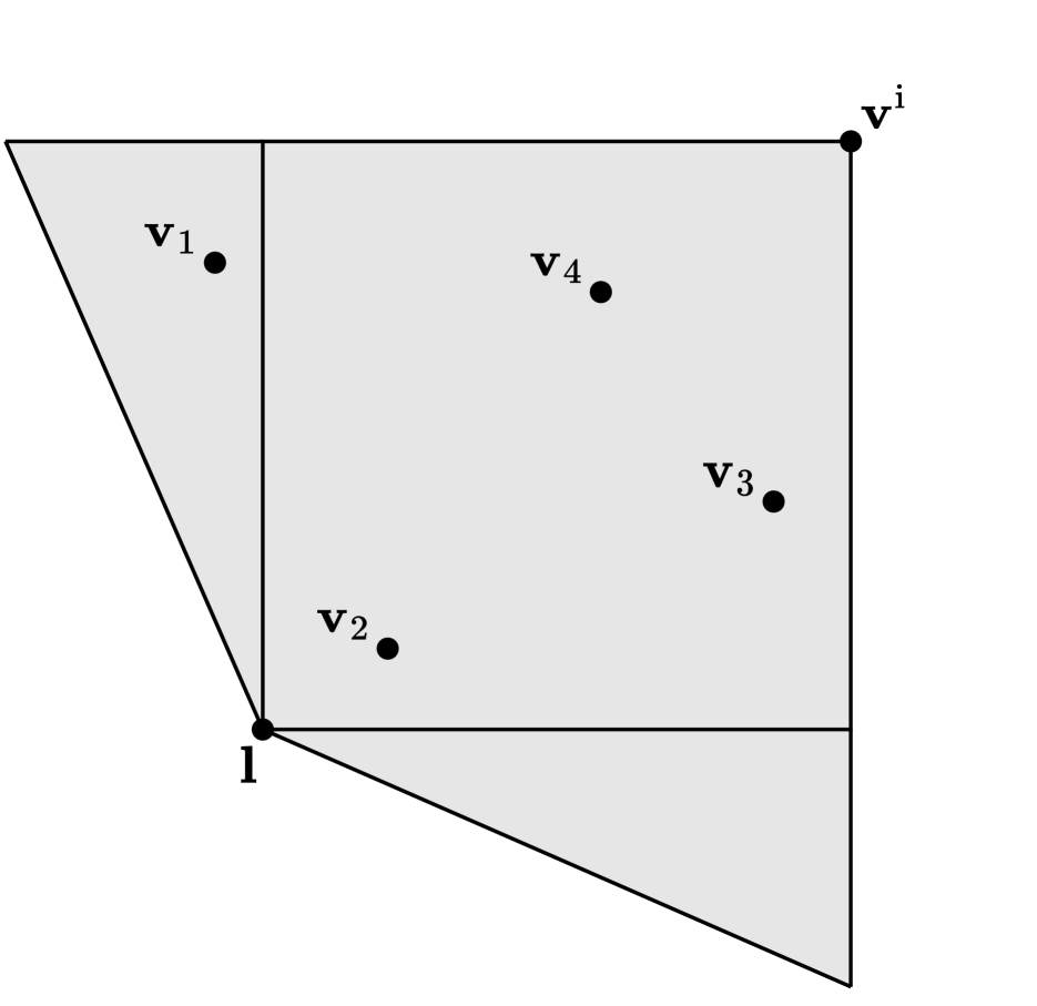
(a)

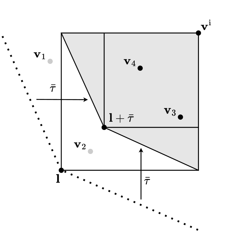
(b)

Figure 5: (a) A possible non-negative set (shaded) for an order approximating ASF with referent ${\bm{l}}$. (b) Shifting ${\bm{l}}$ by $\bar{\tau}$ ensures that all feasible solutions with non-negative values are in the box $B({\bm{l}},{\bm{v}}^{\text{i}})$.

Let us now show that the Pareto oracle $\Omega^{\tau}({\bm{r}})=\operatorname*{arg\,max}_{\pi\in\Pi}s_{{\bm{r}}+\tau}({\bm{v}}^{\pi})$ with $\tau>\bar{\tau}$ functions as required for the referent ${\bm{l}}$. Assume there exists a Pareto optimal optimal $\pi^{\prime}$ with expected return ${\bm{v}}^{\prime}$ such that ${\bm{v}}^{\prime}\succeq{\bm{l}}+\tau$. Then $s_{{\bm{l}}+\tau}({\bm{v}}^{\prime})\geq 0$ and therefore the maximisation will return a non-negative solution $\pi^{\ast}$ with expected returns ${\bm{v}}^{\ast}$. By the definition of $\bar{\tau}$ we know that all feasible solutions $\pi$ with non-negative value $s_{{\bm{l}}+\tau}({\bm{v}}^{\pi})$ satisfy the condition ${\bm{v}}^{\pi}\succeq{\bm{l}}+(\tau-\bar{\tau})$ and therefore ${\bm{v}}^{\ast}\succeq{\bm{l}}+(\tau-\bar{\tau})$. Moreover, as the ASF is guaranteed to be strongly increasing, there exists no policy $\pi$ such that ${\bm{v}}^{\pi}\succ{\bm{v}}^{\ast}$ and therefore $\pi^{\ast}$ is Pareto optimal.

Given the lower bound ${\bm{l}}$, for all referents ${\bm{r}}$ such that ${\bm{r}}\succeq{\bm{l}}$ and with $\tau>\bar{\tau}$, the Pareto oracle remains valid. To see this, observe that ${\bm{r}}={\bm{l}}+{\bm{x}}$ where ${\bm{x}}$ is now a non-negative vector. Then,

$$\begin{split}&\left({\bm{l}}+\tau+\mathbb{R}^{d}_{\delta}\right)\cap\{{\bm{v}}\in\mathbb{R}^{d}\mid{\bm{v}}^{\text{i}}\succeq{\bm{v}}\}\subseteq B({\bm{l}},{\bm{v}}^{\text{i}})\\ \implies&\left({\bm{l}}+\tau+\mathbb{R}^{d}_{\delta}\right)\cap\{{\bm{v}}\in\mathbb{R}^{d}\mid{\bm{v}}^{\text{i}}-{\bm{x}}\succeq{\bm{v}}\}\subseteq B({\bm{l}},{\bm{v}}^{\text{i}}-{\bm{x}}).\end{split}$$ (14)

This implication can be shown by contradiction. Assume that,

$$\exists{\bm{v}}\in\left({\bm{l}}+\tau+\mathbb{R}^{d}_{\delta}\right)\cap\{{\bm{v}}\in\mathbb{R}^{d}\mid{\bm{v}}^{\text{i}}-{\bm{x}}\succeq{\bm{v}}\}\text{ and }{\bm{v}}\notin B({\bm{l}},{\bm{v}}^{\text{i}}-{\bm{x}}).$$ (15)

However, by definition of ${\bm{v}}$, ${\bm{v}}^{\text{i}}-{\bm{x}}\succeq{\bm{v}}$ and

$${\bm{v}}\in\left({\bm{l}}+\tau+\mathbb{R}^{d}_{\delta}\right)\cap\{{\bm{v}}\in\mathbb{R}^{d}\mid{\bm{v}}^{\text{i}}-{\bm{x}}\succeq{\bm{v}}\}$$

$$\implies {\bm{v}}\in\left({\bm{l}}+\tau+\mathbb{R}^{d}_{\delta}\right)\cap\{{\bm{v}}\in\mathbb{R}^{d}\mid{\bm{v}}^{\text{i}}\succeq{\bm{v}}\}$$

$$\implies {\bm{v}}\in B({\bm{l}},{\bm{v}}^{\text{i}})$$

$$\implies {\bm{v}}\succeq{\bm{l}}.$$

As ${\bm{v}}\succeq{\bm{l}}$ and ${\bm{v}}^{\text{i}}-{\bm{x}}\succeq{\bm{v}}$ this implies ${\bm{v}}\in B({\bm{l}},{\bm{v}}^{\text{i}}-{\bm{x}})$, which is a contradiction. Therefore $\left({\bm{l}}+\tau+\mathbb{R}^{d}_{\delta}\right)\cap\{{\bm{v}}\in\mathbb{R}^{d}\mid{\bm{v}}^{\text{i}}-{\bm{x}}\succeq{\bm{v}}\}\subseteq B({\bm{l}},{\bm{v}}^{\text{i}}-{\bm{x}})$. By a rigid transformation and recalling that ${\bm{r}}={\bm{l}}+{\bm{x}}$, we obtain,

$$\left({\bm{r}}+\tau+\mathbb{R}^{d}_{\delta}\right)\cap\{{\bm{v}}\in\mathbb{R}^{d}\mid{\bm{v}}^{\text{i}}\succeq{\bm{v}}\}\subseteq B({\bm{r}},{\bm{v}}^{\text{i}}).$$ (16)

We can subsequently apply the same reasoning to establish the validity of the Pareto oracle for the lower bound ${\bm{l}}$ to all dominating referents ${\bm{r}}$. ∎

C.2 Alternative Pareto Oracles

To conclude the theoretical results for Pareto oracles, we demonstrate that both convex MDPs and constrained MDPs may be leveraged to implement them.

Convex MDPs. A convex Markov decision process is a generalisation of an MDP, where an agent seeks to minimise a convex function (or equivalently maximise a concave function) over a convex set of admissible occupancy measures. Let $\mathcal{K}_{\gamma}$ be the set of discounted state occupancy measures for some discount factor $\gamma$. The expected return ${\bm{v}}^{\pi}$ of some policy $\pi$ can be written as a linear function of the occupancy measure of the policy $d_{\pi}$ and the reward function of the MDP, ${\bm{v}}^{\pi}=\sum_{s,a}\bm{\mathcal{R}}(s,a)d_{\pi}(s,a)$. Corollary C.3 then follows immediately.

Corollary C.3.

Let $\bm{\mathcal{M}}=\langle\mathcal{S},\mathcal{A},\mathbf{P},\bm{\mathcal{R}},\allowbreak\mu,\gamma\rangle$ be a MOMDP with $d$ objectives. For a given oracle tolerance $\tau\geq 0$ and referent ${\bm{r}}$, we define a convex MDP $\mathcal{M}_{\text{conv}}$ with the same states, actions, transition function, discount factor and initial state distribution as $\bm{\mathcal{M}}$. For $s_{\bm{r}}$ defined in Equation 2 and $\Pi$ the set of stochastic policies, $\Omega^{\tau}({\bm{r}})=\operatorname*{arg\,max}_{d_{\pi}\in\mathcal{K}_{\gamma}}s_{{\bm{r}}+\tau}({\bm{v}}^{\pi})$ is a valid weak or approximate Pareto oracle.

Proof.

Since Equation 2 is concave for any referent ${\bm{r}}$ and the composition of a linear function and concave function preserves concavity, the problem is concave. Furthermore, $\mathcal{K}_{\gamma}$ is by definition a convex polytope for the set of stochastic policies. As such, $\mathcal{M}_{\text{conv}}$ is a convex MDP and since $s_{\bm{r}}$ can be constructed as both an order representing and order approximating achievement scalarising function, Theorem 5.3 and Theorem 5.4 can be applied. ∎

This reformulation enables the use of techniques with strong theoretical guarantees. For instance, Zhang et al. (2020) propose a policy gradient method that converges to the global optimum, and Zahavy et al. (2021) introduce a meta-algorithm using standard RL algorithms that converges to the optimal solution with any tolerance, assuming reasonably low-regret algorithms. Additionally, it has been demonstrated that for any convex MDP, a mean-field game can be constructed, for which any Nash equilibrium in the game corresponds to an optimum in the convex MDP (Geist et al., 2022).

Constrained MDPs. A constrained Markov decision process $\mathcal{M}_{\text{const}}$ is an MDP, augmented with a set of $m$ auxiliary cost functions $C_{j}:\mathcal{S}\times\mathcal{A}\times\mathcal{S}\to\mathbb{R}$ and related limit $c_{j}$. Let $J_{C_{j}}(\pi)$ denote the expected discounted return of policy $\pi$ for the auxiliary cost function $C_{j}$. The feasible policies from a given class of policies $\Pi$ is then $\Pi_{C}=\{\pi\in\Pi\mid\forall i,J_{C_{j}}(\pi)\geq c_{j}\}$. Finally, the reinforcement learning problem in a CMDP is as follows,

$$\pi^{\ast}=\operatorname*{arg\,max}_{\pi\in\Pi_{C}}v^{\pi}.$$ (17)

We demonstrate that an approximate Pareto oracle can be implemented by solving an auxiliary constrained MDP, where the constraints ensure that the target region is respected and the scalar reward function is designed such that only Pareto optimal policies are returned as the optimal solution. Importantly, since constrained MDPs have no inherent tolerance, the user is free to select any tolerance $\tau>0$.

Corollary C.4.

Let $\bm{\mathcal{M}}=\langle\mathcal{S},\mathcal{A},\mathbf{P},\bm{\mathcal{R}},\allowbreak\mu,\gamma\rangle$ be a MOMDP with $d$ objectives. For a given oracle tolerance $\tau>0$ and referent ${\bm{r}}$, we define a constrained MDP $\mathcal{M}_{\text{const}}$ with the same states, actions, transition function, discount factor and initial state distribution as $\bm{\mathcal{M}}$. $\mathcal{M}_{\text{const}}$ has $d$ cost functions corresponding to the original $d$ reward function with limits ${\bm{r}}+\tau$ and the scalar reward function is the sum of the original reward vector. Then $\Omega^{\tau}({\bm{r}})=\operatorname*{arg\,max}_{\pi\in\Pi_{C}}v^{\pi}$ is a valid approximate Pareto oracle.

Proof.

Assume the construction outlined in the theorem and that there exists a Pareto optimal policy $\pi$ such that ${\bm{v}}^{\pi}\succeq{\bm{r}}+\tau$. Then $\Pi_{C}$ is non-empty and the Pareto oracle $\mathcal{O}^{\tau}({\bm{r}})=\operatorname*{arg\,max}_{\pi\in\Pi_{C}}v^{\pi}$ returns a Pareto optimal policy $\pi^{\ast}$ with expected return ${\bm{v}}^{\ast}$ such that ${\bm{v}}^{\ast}\succeq{\bm{r}}+\tau$. If $\pi^{\ast}$ is not Pareto optimal, there exists a policy $\pi^{\prime}$ with expected return ${\bm{v}}^{\prime}$ such that ${\bm{v}}^{\prime}\succ{\bm{v}}^{\ast}$. This then implies that,

$$\sum_{j\in\{1,\dots,d\}}v^{\prime}_{j}>\sum_{j\in\{1,\dots,d\}}v^{\ast}_{j}$$ (18)

which leads to a contradiction. ∎

Appendix D Experiment Details

In this section, we provide details concerning the experimental evaluation presented in Section 7. Concretely, we discuss the selection of baselines and environments, provide the concrete evaluation setup used in our experiments and show complete results including Envelope Q-learning which was omitted from the main text.

D.1 Baselines

Since IPRO is the first general-purpose method capable of learning a Pareto front of arbitrary policies in general MOMDPs, we select baselines that specialise for a subset of environments that we evaluate on. We now discuss these baselines and highlight their intended use case.

Convex hull algorithms. We consider two state-of-the-art convex hull algorithms, Generalised Policy Improvement - Linear Support (GPI-LS) (Alegre et al., 2023) and Envelope Q-Learning (EQL) (Yang et al., 2019). GPI-LS decomposes the task of learning the convex hull into learning a set of policies at the vertices of the convex hull. EQL on the other hand proposes a new optimality operator for vectorial Q-values, called the envelope optimality operator, and uses this to learn deep vectorial Q-networks. To ensure a fair comparison between IPRO and the convex hull algorithms, we retain all Pareto optimal policies generated by them during evaluation rather than only the policies in the convex hull. Moreover, in both Minecart and MO-Reacher the Pareto front is mostly convex, further supporting this comparison.

Pareto front algorithm. As a direct comparison to IPRO, we select Pareto Conditioned Networks (PCN) which is specifically designed to learn a Pareto front of deterministic policies in deterministic MOMDPs (Reymond et al., 2022). PCN trains a single neural network on a range of desired trade-offs, to generalise over the full set of Pareto optimal policies. This is achieved by learning to predict the “return-to-go” from any state and selecting the action that most closely reaches the returns of the chosen trade-off. We note that, while Deep Sea Treasure and MO-Reacher are deterministic environments, Minecart is not, which may explain PCN’s worse performance in this environment.

D.2 Environments

To focus solely on IPRO’s performance, we initialise each experiment with predefined minimal and maximal points to establish the bounding box of the environment. It is important to emphasise that these points can be obtained using conventional reinforcement learning algorithms without requiring any modifications, justifying their omission from our evaluation process.

Deep Sea Treasure (DST). We initialise IPRO with $(124,-50)$ and $(0,0)$ as the maximal points and give $(0,-50)$ as the only minimal point. We set the discount factor to $1$, signifying no discounting, and maintain a fixed time horizon of $50$ timesteps for each episode. The hypervolumes shown in Figure 3 were calculated using $(0,-50)$ as the reference point. We note that we one-hot encode the observations due to the discrete nature of the state space. Finally, a tolerance $\tau$ of $0$ was set to allow IPRO to find the complete Pareto front in this environment.

Minecart. In the Minecart environment, we set $\gamma=0.98$ to align with related work. For minimal points, IPRO is initialised with the nadir $(-1,-1,-200)$ for each dimension. For maximal points, we consider the nadir and set each dimension to its theoretical maximum: $(1.5,-1,-200),(-1,1.5,-200),(-1,-1,0)$. Our reference point is also the nadir and the time horizon is 1000. A tolerance of $1\times 10^{-15}$ was used.

MO-Reacher. In the Reacher environment, we use $(-50,-50,-50,-50)$ in each dimension as the minimal points, and similarly, set this vector to 40 for each dimension for the maximal points. The discount factor $\gamma$ is set to $0.99$. The reference point is again set to the nadir, a time horizon of 50 was used and tolerance was set to $1\times 10^{-15}$.

D.3 Extended Results

In the main text of Section 7 we omitted the results for EQL since it performed worse than GPI-LS on all environments and metrics. For completeness, we provide in Figure 6 and Table 2 the same metrics but now including EQL.

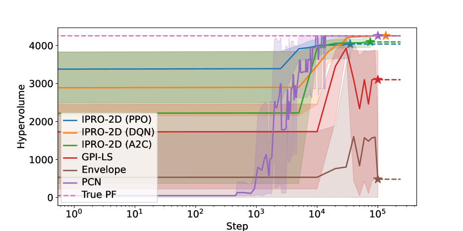
(a) Deep Sea Treasure

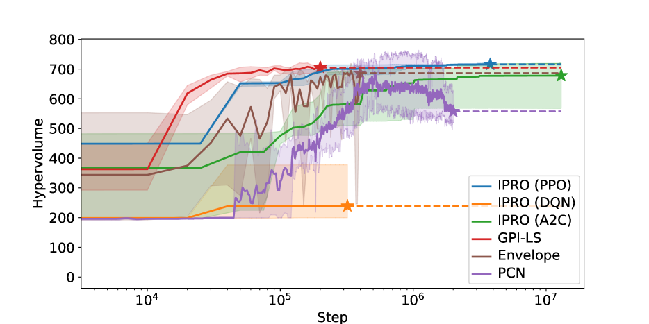
(b) Minecart

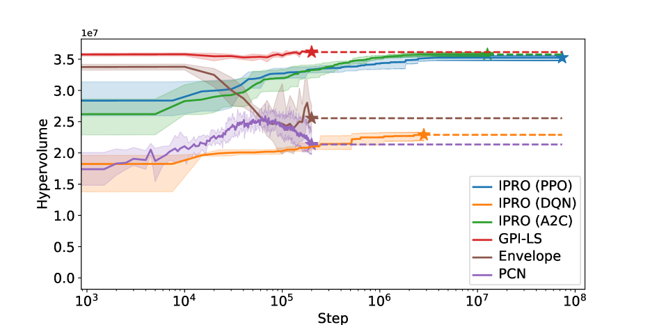
(c) MO-Reacher

Figure 6: The mean hypervolume with 95-percentile interval over time. Stars indicate when each algorithm finished and lines are extended to better compare final values. The pretraining phase of IPRO is not shown. We note that the x-axis is on a log scale.

Table 2: The minimum $\varepsilon$ shift necessary to obtain any undiscovered Pareto optimal solution. The best mean is in bold.

Env	Algorithm	$\varepsilon$
	IPRO (PPO)	$5.40\pm 2.58$
	IPRO (A2C)	$4.20\pm 1.83$
DST	IPRO (DQN)	$\bm{0.00\pm 0.00}$
	PCN	$\bm{0.00\pm 0.00}$
	GPI-LS	$32.60\pm 45.20$
	Envelope	$108.80\pm 29.41$
	IPRO (PPO)	$0.66\pm 0.07$
	IPRO (A2C)	$0.54\pm 0.11$
Minecart	IPRO (DQN)	$1.14\pm 0.01$
	PCN	$0.67\pm 0.12$
	GPI-LS	$\bm{0.28\pm 0.09}$
	Envelope	$0.30\pm 0.10$
	IPRO (PPO)	$5.45\pm 1.22$
	IPRO (A2C)	$\bm{2.65\pm 0.38}$
MO-Reacher	IPRO (DQN)	$14.78\pm 1.43$
	PCN	$18.24\pm 2.52$
	GPI-LS	$5.28\pm 0.56$
	Envelope	$14.38\pm 1.21$

D.4 Evaluation Setup

To conclude this section, we provide the methodology for computing the metrics we reported in the main text and give precise hyperparameter values for our experiments.

D.4.1 Metrics

In Section 7 we first evaluate all algorithms on their hypervolume which measures the total volume of vectors dominated by solutions on the Pareto front with respect to some reference point. While this is a popular metric in MORL, it is heavily influenced by the choice of reference point and may give a distorted perspective of the actual quality of the learned Pareto front. To better gauge this quality, we compute for each algorithm and each run the minimum $\varepsilon$ shift necessary to obtain any Pareto optimal solution obtained by another algorithm. Intuitively, a lower $\varepsilon$ signifies a smaller loss on all objectives and therefore indicates a higher quality of the Pareto front compared to other algorithms. Let ${\mathcal{V}}^{\text{alg}}$ be the Pareto front obtained by some algorithm in a particular run and let $\hat{{\mathcal{V}}}$ be the union of Pareto fronts across all algorithms and runs. Then the $\varepsilon$ metric for ${\mathcal{V}}^{\text{alg}}$ is computed as shown in Equation 19.

$$\min\left\{\varepsilon\geq 0\mid\forall{\bm{v}}\in\hat{}{\mathcal{V}},\exists{\bm{v}}^{\prime}\in{\mathcal{V}}^{\text{alg}}:\|{\bm{v}}-{\bm{v}}^{\prime}\|_{\infty}\leq\varepsilon\right\}$$ (19)

D.4.2 Hyperparameters

In Table 3 we provide a description of all hyperparameters used in our Pareto oracles and the algorithms for which they apply. Finally, in Tables 4, 5 and 6 we give the hyperparameter values used in our reported experiments.

Table 3: A description of the relevant hyperparameters.

Parameter	Algorithm	Description
scale	DQN, A2C, PPO	Scale the output of Equation 2 to generate a greater learning signal
$\rho$	DQN, A2C, PPO	Augmentation parameter from Equation 2
pretrain_iters	DQN, A2C, PPO	The number of pretraining iterations
num_referents	DQN, A2C, PPO	The number of additional referents to sample while updating during pretraining
pretraining_steps	DQN, A2C, PPO	Number of global steps while pretraining
online_steps	DQN, A2C, PPO	Number of global steps while learning online
critic_hidden	DQN, A2C, PPO	Number of hidden neurons per layer for the critic
lr_critic	DQN, A2C, PPO	The learning rate for the critic
actor_hidden	A2C, PPO	Number of hidden neurons per layer for the actor
lr_actor	A2C, PPO	Learning rate for the actor
n_steps	A2C, PPO	Number of environment interactions before each update
gae_lambda	A2C, PPO	$\lambda$ parameter for generalised advantage estimation
normalise_advantage	A2C, PPO	Normalise the advantage
e_coef	A2C, PPO	Entropy loss coefficient to compute the overall loss
v_coef	A2C, PPO	Value loss coefficient to compute the overall loss
max_grad_norm	A2C, PPO	Maximum gradient norm
clip_coef	PPO	Clip coefficient used in the PPO surrogate objective
num_envs	PPO	Number of parallel environments to run in
anneal_lr	PPO	Anneal the learning rate over time
clip_range_vf	PPO	Clipping range for the value function
update_epochs	PPO	Number of update epochs to execute
num_minibatches	PPO	Number of minibatches to divide a batch in
batch_size	DQN	Batch size for each update
buffer_size	DQN	Size of the replay buffer
soft_update	DQN	Multiplication factor for the soft update
pre_epsilon_start	DQN	Pretraining starting exploration probability
pre_epsilon_end	DQN	Pretraining final exploration probability
pre_exploration_frac	DQN	Pretraining exploration fraction of total timesteps
pre_learning_start	DQN	Pretraining start of learning
online_epsilon_start	DQN	Online starting exploration probability
online_epsilon_end	DQN	Online final exploration probability
online_exploration_frac	DQN	Online exploration fraction of total timesteps
online_learning_start	DQN	Online start of learning

Table 4: The hyperparameters used in the DQN oracles.

Parameter	DST	Minecart	MO-Reacher
scale	100	100	10
$\rho$	0.01	0.01	0.01
pretrain_iters	50	50	50
num_referents	4	32	16
online_steps	5.0e+03	2.0e+04	7.5e+03
pretraining_steps	5.0e+03	2.0e+04	7.5e+03
critic_hidden	(128,)	(256, 256, 256, 256)	(256, 256, 256, 256)
lr_critic	0.0006	0.0001	0.0007
batch_size	16	32	16
buffer_size	1.0e+04	1.0e+05	1.0e+05
soft_update	0.1	0.1	0.1
pre_learning_start	100	1.0e+03	1.0e+03
pre_epsilon_start	1	0.75	0.5
pre_epsilon_end	0.05	0.2	0.1
pre_exploration_frac	0.5	0.75	0.75
online_learning_start	100	100	100
online_epsilon_start	1	0.5	0.5
online_epsilon_end	0.05	0.1	0.05
online_exploration_frac	0.3	0.25	0.5

Table 5: The hyperparameters used in the A2C oracles.

Parameter	DST	Minecart	MO-Reacher
scale	100	100	100
$\rho$	0.01	0.01	0.01
pretrain_iters	75	75	75
num_referents	16	16	16
online_steps	5.0e+03	2.5e+04	5.0e+03
pretraining_steps	2.5e+03	7.5e+04	2.5e+04
critic_hidden	(128,)	(128, 128, 128)	(64, 64)
lr_critic	0.001	0.0001	0.0007
actor_hidden	(128,)	(128, 128, 128)	(64, 64)
lr_actor	0.0001	0.0001	0.001
n_steps	16	32	16
gae_lambda	0.95	0.95	0.95
normalise_advantage	False	False	False
e_coef	0.01	0.1	0.1
v_coef	0.5	0.5	0.1
max_grad_norm	0.5	50	1

Table 6: The hyperparameters used in the PPO oracles.

Parameter	DST	Minecart	MO-Reacher
scale	100	100	100
$\rho$	0.01	0.01	0.01
pretrain_iters	25	100	100
num_referents	4	32	8
online_steps	2.5e+03	2.5e+04	7.5e+03
pretraining_steps	2.5e+03	2.0e+04	1.5e+04
critic_hidden	(256,)	(256, 256)	(128, 128, 128)
lr_critic	0.0001	0.0001	0.001
actor_hidden	(256,)	(256, 256)	(128, 128, 128)
lr_actor	0.0007	0.0001	0.0003
n_steps	64	32	64
gae_lambda	0.95	0.95	0.95
normalise_advantage	False	False	False
e_coef	0	0.1	0.1
v_coef	0.5	0.1	0.1
max_grad_norm	5	50	5
clip_coef	0.2	0.1	0.2
num_envs	8	16	8
anneal_lr	False	False	False
clip_range_vf	0.2	0.5	0.2
update_epochs	4	16	4
num_minibatches	4	4	4

References

- Abdolmaleki et al. (2020) Abdolmaleki, A., Huang, S., Hasenclever, L., Neunert, M., Song, F., Zambelli, M., Martins, M., Heess, N., Hadsell, R., and Riedmiller, M. A distributional view on multi-objective policy optimization. In III, H. D. and Singh, A. (eds.), Proceedings of the 37th International Conference on Machine Learning, volume 119, pp. 11–22. PMLR, 2020.
- Abels et al. (2019) Abels, A., Roijers, D. M., Lenaerts, T., Nowé, A., and Steckelmacher, D. Dynamic Weights in Multi-Objective Deep Reinforcement Learning. In Chaudhuri, K. and Salakhutdinov, R. (eds.), Proceedings of the 36th International Conference on Machine Learning, volume 97, pp. 11–20, Long Beach, California, USA, 2019. PMLR.
- Achiam et al. (2017) Achiam, J., Held, D., Tamar, A., and Abbeel, P. Constrained policy optimization. In Precup, D. and Teh, Y. W. (eds.), Proceedings of the 34th International Conference on Machine Learning, volume 70 of Proceedings of Machine Learning Research, pp. 22–31. PMLR, August 2017.
- Alegre et al. (2023) Alegre, L. N., Roijers, D. M., Nowé, A., Bazzan, A. L. C., and da Silva, B. C. Sample-efficient multi-objective learning via generalized policy improvement prioritization. In Proc. of the 22nd International Conference on Autonomous Agents and Multiagent Systems (AAMAS), 2023.
- Altman (1999) Altman, E. Constrained Markov Decision Processes. Routledge, Boca Raton, 1 edition, 1999. ISBN 978-1-315-14022-3. doi: 10.1201/9781315140223.
- Castelletti et al. (2013) Castelletti, A., Pianosi, F., and Restelli, M. A multiobjective reinforcement learning approach to water resources systems operation: Pareto frontier approximation in a single run. Water Resources Research, 49(6):3476–3486, 2013. doi: 10.1002/wrcr.20295.
- Chatterjee et al. (2006) Chatterjee, K., Majumdar, R., and Henzinger, T. A. Markov decision processes with multiple objectives. In Durand, B. and Thomas, W. (eds.), STACS 2006, pp. 325–336, Berlin, Heidelberg, 2006. Springer Berlin Heidelberg. ISBN 978-3-540-32288-7.
- Delgrange et al. (2020) Delgrange, F., Katoen, J.-P., Quatmann, T., and Randour, M. Simple strategies in multi-objective MDPs. In Biere, A. and Parker, D. (eds.), Tools and Algorithms for the Construction and Analysis of Systems, pp. 346–364, Cham, 2020. Springer International Publishing. ISBN 978-3-030-45190-5.
- Ding et al. (2021) Ding, D., Wei, X., Yang, Z., Wang, Z., and Jovanovic, M. Provably efficient safe exploration via primal-dual policy optimization. In Banerjee, A. and Fukumizu, K. (eds.), Proceedings of the 24th International Conference on Artificial Intelligence and Statistics, volume 130 of Proceedings of Machine Learning Research, pp. 3304–3312. PMLR, April 2021.
- Geist et al. (2022) Geist, M., Pérolat, J., Laurière, M., Elie, R., Perrin, S., Bachem, O., Munos, R., and Pietquin, O. Concave utility reinforcement learning: The mean-field game viewpoint. In Proceedings of the 21st International Conference on Autonomous Agents and Multiagent Systems, AAMAS ’22, pp. 489–497, Richland, SC, 2022. International Foundation for Autonomous Agents and Multiagent Systems. ISBN 978-1-4503-9213-6.
- Hayes et al. (2022) Hayes, C. F., Rădulescu, R., Bargiacchi, E., Källström, J., Macfarlane, M., Reymond, M., Verstraeten, T., Zintgraf, L. M., Dazeley, R., Heintz, F., Howley, E., Irissappane, A. A., Mannion, P., Nowé, A., Ramos, G., Restelli, M., Vamplew, P., and Roijers, D. M. A practical guide to multi-objective reinforcement learning and planning. Autonomous Agents and Multi-Agent Systems, 36(1):26, April 2022. ISSN 1573-7454. doi: 10.1007/s10458-022-09552-y.
- Legriel et al. (2010) Legriel, J., Le Guernic, C., Cotton, S., and Maler, O. Approximating the pareto front of multi-criteria optimization problems. In Esparza, J. and Majumdar, R. (eds.), Tools and Algorithms for the Construction and Analysis of Systems, pp. 69–83, Berlin, Heidelberg, 2010. Springer Berlin Heidelberg. ISBN 978-3-642-12002-2.
- Lu et al. (2023) Lu, H., Herman, D., and Yu, Y. Multi-objective reinforcement learning: Convexity, stationarity and pareto optimality. In The Eleventh International Conference on Learning Representations, 2023.
- Meng et al. (2023) Meng, W., Zheng, Q., Pan, G., and Yin, Y. Off-policy proximal policy optimization. Proceedings of the AAAI Conference on Artificial Intelligence, 37(8):9162–9170, June 2023. doi: 10.1609/aaai.v37i8.26099.
- Miettinen (1998) Miettinen, K. Nonlinear Multiobjective Optimization, volume 12 of International Series in Operations Research & Management Science. Springer US, Boston, MA, 1998. ISBN 978-1-4613-7544-9 978-1-4615-5563-6. doi: 10.1007/978-1-4615-5563-6.
- Mnih et al. (2015) Mnih, V., Kavukcuoglu, K., Silver, D., Rusu, A. A., Veness, J., Bellemare, M. G., Graves, A., Riedmiller, M., Fidjeland, A. K., Ostrovski, G., Petersen, S., Beattie, C., Sadik, A., Antonoglou, I., King, H., Kumaran, D., Wierstra, D., Legg, S., and Hassabis, D. Human-level control through deep reinforcement learning. Nature, 518(7540):529–533, 2015. doi: 10.1038/nature14236.
- Mnih et al. (2016) Mnih, V., Badia, A. P., Mirza, L., Graves, A., Harley, T., Lillicrap, T. P., Silver, D., and Kavukcuoglu, K. Asynchronous methods for deep reinforcement learning. In Balcan, M. F. and Weinberger, K. Q. (eds.), 33rd International Conference on Machine Learning, ICML 2016, volume 4, pp. 2850–2869, New York, New York, USA, September 2016. PMLR. ISBN 978-1-5108-2900-8.
- Nikulin et al. (2012) Nikulin, Y., Miettinen, K., and Mäkelä, M. M. A new achievement scalarizing function based on parameterization in multiobjective optimization. OR Spectrum, 34(1):69–87, January 2012. ISSN 1436-6304. doi: 10.1007/s00291-010-0224-1.
- Papadimitriou & Yannakakis (2000) Papadimitriou, C. and Yannakakis, M. On the approximability of trade-offs and optimal access of Web sources. In Proceedings 41st Annual Symposium on Foundations of Computer Science, pp. 86–92, November 2000. doi: 10.1109/SFCS.2000.892068.
- Reymond et al. (2022) Reymond, M., Bargiacchi, E., and Nowé, A. Pareto conditioned networks. In Proceedings of the 21st International Conference on Autonomous Agents and Multiagent Systems, AAMAS ’22, pp. 1110–1118, Richland, SC, 2022. International Foundation for Autonomous Agents and Multiagent Systems. ISBN 978-1-4503-9213-6.
- Reymond et al. (2023) Reymond, M., Hayes, C. F., Steckelmacher, D., Roijers, D. M., and Nowé, A. Actor-critic multi-objective reinforcement learning for non-linear utility functions. Autonomous Agents and Multi-Agent Systems, 37(2):23, April 2023. ISSN 1573-7454. doi: 10.1007/s10458-023-09604-x.
- Roijers & Whiteson (2017) Roijers, D. M. and Whiteson, S. Multi-objective decision making. In Synthesis Lectures on Artificial Intelligence and Machine Learning, volume 34, pp. 129–129. Morgan and Claypool, 2017. ISBN 978-1-62705-960-2. doi: 10.2200/S00765ED1V01Y201704AIM034.
- Schulman et al. (2017) Schulman, J., Wolski, F., Dhariwal, P., Radford, A., and Klimov, O. Proximal policy optimization algorithms. arXiv preprint arXiv:1707.06347, 2017.
- Schulman et al. (2018) Schulman, J., Moritz, P., Levine, S., Jordan, M., and Abbeel, P. High-dimensional continuous control using generalized advantage estimation, 2018.
- Siddique et al. (2020) Siddique, U., Weng, P., and Zimmer, M. Learning fair policies in multi-objective (Deep) reinforcement learning with average and discounted rewards. In III, H. D. and Singh, A. (eds.), Proceedings of the 37th International Conference on Machine Learning, volume 119 of Proceedings of Machine Learning Research, pp. 8905–8915. PMLR, July 2020.
- Vamplew et al. (2011) Vamplew, P., Dazeley, R., Berry, A., Issabekov, R., and Dekker, E. Empirical evaluation methods for multiobjective reinforcement learning algorithms. Machine Learning, 84(1):51–80, 2011. doi: 10.1007/s10994-010-5232-5.
- Van Moffaert et al. (2013) Van Moffaert, K., Drugan, M. M., and Nowé, A. Scalarized multi-objective reinforcement learning: Novel design techniques. In 2013 IEEE Symposium on Adaptive Dynamic Programming and Reinforcement Learning (ADPRL), pp. 191–199, 2013. doi: 10.1109/ADPRL.2013.6615007.
- Wierzbicki (1982) Wierzbicki, A. P. A mathematical basis for satisficing decision making. Mathematical Modelling, 3(5):391–405, 1982. ISSN 0270-0255. doi: 10.1016/0270-0255(82)90038-0.
- Xu et al. (2020) Xu, J., Tian, Y., Ma, P., Rus, D., Sueda, S., and Matusik, W. Prediction-Guided Multi-Objective Reinforcement Learning for Continuous Robot Control. In III, H. D. and Singh, A. (eds.), Proceedings of the 37th International Conference on Machine Learning, volume 119, pp. 10607–10616. PMLR, 2020.
- Yang et al. (2019) Yang, R., Sun, X., and Narasimhan, K. A generalized algorithm for multi-objective reinforcement learning and policy adaptation. In Proceedings of the 33rd International Conference on Neural Information Processing Systems. Curran Associates Inc., Red Hook, NY, USA, 2019.
- Zahavy et al. (2021) Zahavy, T., O’Donoghue, B., Desjardins, G., and Singh, S. Reward is enough for convex MDPs. In Beygelzimer, A., Dauphin, Y., Liang, P., and Vaughan, J. W. (eds.), Advances in Neural Information Processing Systems, 2021.
- Zhang et al. (2020) Zhang, J., Koppel, A., Bedi, A. S., Szepesvari, C., and Wang, M. Variational policy gradient method for reinforcement learning with general utilities. In Larochelle, H., Ranzato, M., Hadsell, R., Balcan, M., and Lin, H. (eds.), Advances in Neural Information Processing Systems, volume 33, pp. 4572–4583. Curran Associates, Inc., 2020.
- Zhang & Li (2007) Zhang, Q. and Li, H. MOEA/D: A multiobjective evolutionary algorithm based on decomposition. IEEE Transactions on Evolutionary Computation, 11(6):712–731, December 2007. ISSN 1941-0026. doi: 10.1109/TEVC.2007.892759.