Quantum geometric bound for saturated ferromagnetism

Abstract

Despite its abundance in nature, predicting the occurrence of ferromagnetism in the ground state is possible only under very limited conditions such as in a flat band system with repulsive interaction or in a band with a single hole under infinitely large Coulomb repulsion, etc. Here, we propose a general condition to achieve saturated ferromagnetism based on the quantum geometry of electronic wave functions in itinerant electron systems. By analyzing multi-band repulsive Hubbard models with an integer band filling, relevant to either ferromagnetic insulators or semimetals, we propose a rigorous quantum geometric upper bound on the spin stiffness. By employing this geometric bound, we establish that saturated ferromagnetism is prohibited in the absence of interband coupling, even when the local Hubbard repulsion is infinitely large. As a corollary, this shows that saturated ferromagnetism is forbidden in any half-filled Hubbard model. We also derive the condition that the upper bound of the spin stiffness can be completely characterized by the Abelian quantum metric. We believe that our findings reveal a profound connection between quantum geometry and ferromagnetism, which can be extended to various symmetry-broken ground states in itinerant electronic systems.

Introduction.— Ferromagnetism is the simplest form of symmetry-broken ground states whose fundamental origin has been discussed by divergent perspectives, from Heisenberg’s localized electron picture Heisenberg (1928) to Bloch’s itinerant electron approach Bloch (1929). More recently, the modern theory of ferromagnetism formulated based on the Hubbard model Tasaki (2020) has led to various theorems about itinerant ferromagnetism, including the following two distinct mechanisms. One is Nagaoka’s ferromagnetism Nagaoka (1966); Tasaki (1989, 1998), where a single hole in the valence band induces the spin alignment when the electron repulsion is infinite. The other is flat band ferromagnetism with repulsive interaction, extensively studied by Mielke Mielke (1991) and Tasaki Tasaki (1992). Despite the valuable insights delivered by them, these two representative theorems rely on the highly restrictive form of the kinetic Hamiltonian without the consideration of electronic wave functions inherent in itinerant electronic systems.

Recently, the quantum geometry of electronic wave functions has garnered increasing attention due to its relevance to various physical phenomena, such as anomalous Landau levels of flat bands Rhim et al. (2020); Hwang et al. (2021); Jung et al. (2023), flat band superfluidity Tian et al. (2023); Xie et al. (2020); Liang et al. (2017), and nonlinear Hall effect Gao et al. (2023); Wang et al. (2023), etc. Moreover, it has been shown that quantum geometry plays a prominent role in describing the interacting ground states with spontaneous symmetry breaking. For instance, in superconductors, quantum geometry was shown to be deeply related to the superfluid weight Peotta and Törmä (2015); Xie et al. (2020), the length scale of Cooper pairs Chen and Law (2023); Hu et al. (2023), and the dynamics of the Higgs mode Villegas and Yang (2021). Also, in excitonic ground states, quantum geometry was shown to induce anomalous Lamb shifts Srivastava and Imamoğlu (2015), contribute to the exciton drift velocity Cao et al. (2021), and stabilize exciton condensates Hu et al. (2022). In contrast, the role of quantum geometry in magnetic ground states remains largely unexplored Bernevig et al. (2021); Wu and Das Sarma (2020).

In this Letter, we investigate the effects of quantum geometry on a class of ferromagnetic ground states at integer filling, namely, saturated ferromagnetism, which can appear in itinerant electronic systems where the total spin is maximally polarized. By examining the spin excitations of the Hubbard model, we study the spin stiffness, the inverse effective mass of the gapless magnon generated by breaking continuous spin rotational symmetry. We show that the spin stiffness has an upper bound characterized by the quantum geometry of the non-interacting electronic bands, which shows the prominent role of interband coupling in stabilizing saturated ferromagnetism. Using the relation between this geometric upper bound and the positive-definiteness of the spin stiffness, we derive a no-go theorem for saturated ferromagnetism. Explicitly, we show that saturated ferromagnetism is strictly prohibited in the absence of the interband coupling. This immediately implies that saturated ferromagnetism is forbidden in any half-filled Hubbard model. We also derive the condition that the geometric upper bound can be completely characterized by the Abelian quantum metric, directly demonstrating its relation with quantum geometry.

Saturated ferromagnetism.— Saturated ferromagnetism represents the most robust manifestation of ferromagnetic behavior, characterized by the ground state possessing maximum total spin. The highly restricted form of this configuration allows us to represent the ground state using only the information of the kinetic Hamiltonian, considerably simplifying the problem Tasaki (2020). For its description, let us consider the following repulsive Hubbard model

$$H=\sum_{{\bm{k}}}^{N_{c}}\sum_{\alpha,\beta}^{N_{orb}}\sum_{\sigma}^{\uparrow,\downarrow}h({\bm{k}})_{\alpha\beta}c^{\dagger}_{{\bm{k}}\alpha\sigma}c_{{\bm{k}}\beta\sigma}+U\sum_{i}^{N_{c}}n_{i\alpha\uparrow}n_{i\alpha\downarrow},$$ (1)

where $h({\bm{k}})$ and $U>0$ indicate the kinetic Hamiltonian and the local Hubbard repulsion, respectively. $c_{{\bm{k}}\beta\sigma}$ denotes the annihilation operator of an electron with momentum ${\bm{k}}$, orbital index $\alpha=1,\dots,N_{orb}$, and spin $\sigma=\uparrow,\downarrow$. $n_{i\alpha\sigma}\equiv c^{\dagger}_{i\alpha\sigma}c_{i\alpha\sigma}$ is the corresponding number operator. $i=1,\dots,N_{c}$ labels the unit cells. In addition, we define a momentum-independent filling $v\equiv N_{occ}/2N_{orb}$, assuming that $N_{occ}\in\mathbb{Z}$ electrons exist per unit cell, which results in a total of $N_{tot}=N_{c}N_{occ}$ electrons. More detailed information of the model is given in the Supplemental Materials (SM).

Following Ref. Tasaki (2020), we denote the local and total spin operators by ${\bm{S}}_{i\alpha}=\frac{1}{2}\sum_{\sigma_{1},\sigma_{2}}c^{\dagger}_{i\alpha\sigma_{1}}{\bm{\sigma}}_{\sigma_{1}\sigma_{2}}c_{i\alpha\sigma_{2}}$ and ${\bm{S}}_{tot}=\sum_{i\alpha}{\bm{S}}_{i\alpha}$, respectively (${\bm{\sigma}}$ is the Pauli matrix, and we set $\hbar=1$). The system is said to exhibit saturated ferromagnetism if and only if

$$({\bm{S}}_{tot})^{2}|GS\rangle=S_{max}(S_{max}+1)|GS\rangle,$$ (2)

where $S_{max}\equiv\frac{N_{tot}}{2}$, for any ground state $|GS\rangle$. This imposes the constraints that $N_{occ}\in\{1,\dots,N_{orb}\}$, and $v\leq\frac{1}{2}$. A noteworthy feature of saturated ferromagnets is that we can entirely ascertain the eigenspace of the ground state using the noninteracting Hamiltonian Miyahara et al. (2005); Tasaki (2020).

To clarify, let $E_{GS}=min(\sum_{j}^{N_{tot}}\varepsilon_{j})$ be the ground state energy such that $\varepsilon_{j}\in\bigcup_{i}spec\{h({\bm{k}}_{i})\}$, with a degeneracy $d_{0}$. Then, the ground state manifold is a $d_{0}\times(2S_{max}+1)$-fold degenerate eigenspace characterized by $E_{GS}$, where the additional $(2S_{max}+1)$-fold degeneracy arises from the $SU(2)$ symmetry of the Hubbard model. More specifically, let $|GS_{j}\rangle$ ($j=1,\dots,d_{0}$) be fully $\uparrow$-spin polarized states with energy $E_{GS}$. If we define the spin-lowering operator as $S_{tot}^{-}\equiv S_{tot}^{x}-iS_{tot}^{y}$, the states $(S_{tot}^{-})^{m}|GS_{j}\rangle$ ($m\in\{0,\dots,2S_{max}\}$, $j\in\{1,\dots,d_{0}\}$) form a basis of the ground state manifold. Thus, we can perform a $SU(2)$ rotation to express the ground state to be aligned with $\uparrow$-spins. Throughout this letter, we assume such ground state, and denote it by $|\Omega\rangle$. Moreover, $d_{0}=1$ when the kinetic Hamiltonian has no partially occupied band. Then, the ground state can be represented by a single Slater determinant Tasaki (2020), and mean-field theory becomes exact for any $U$. Below, we use the term “ferromagnetism” to mean this specific context unless specified otherwise.

Spin excitations.— Let us describe the spin excitation spectrum of saturated ferromagnets, generally composed of the Stoner continuum and the low-energy magnon modes. Assuming a ground state $|\Omega\rangle$ in which $N_{occ}$ occupied bands are fully $\uparrow$-spin polarized, the spin excitation operator with momentum ${\bm{Q}}$ can be described by

$$\Psi_{\bm{Q}}^{\dagger}=\sum_{{\bm{k}}}^{N_{c}}\sum_{\alpha}^{N_{orb}}\sum_{n}^{N_{occ}}z_{{\bm{k}}\alpha n}({\bm{Q}})c^{\dagger}_{{\bm{k}}+{\bm{Q}}\alpha\downarrow}\phi_{n{\bm{k}}},$$ (3)

where $z_{{\bm{k}}\alpha n}({\bm{Q}})$ is an arbitrary number and $\phi^{\dagger}_{n{\bm{k}}}=\sum_{\alpha}^{N_{orb}}c^{\dagger}_{{\bm{k}}\alpha\uparrow}|u_{n}({\bm{k}})\rangle_{\alpha}$ is the creation operator of the $n$-th occupied band in which $|u_{n}({\bm{k}})\rangle$ is the eigenvector of $h({\bm{k}})$ with eigenvalue $E_{n}({\bm{k}})$. Then, we have $|\Omega\rangle=\prod_{n}^{N_{occ}}\prod_{{\bm{k}}}^{N_{c}}\phi^{\dagger}_{n{\bm{k}}}|0\rangle$, where $|0\rangle$ indicates the vacuum state.

Defining $|{\bm{Q}}\rangle\equiv\Psi_{{\bm{Q}}}^{\dagger}|\Omega\rangle$, the spin excitation energy is given by

$$\mathcal{E}({\bm{Q}})=\frac{\langle{\bm{Q}}|H|{\bm{Q}}\rangle}{\langle{\bm{Q}}|{\bm{Q}}\rangle}-\langle\Omega|H|\Omega\rangle.$$ (4)

We decouple the many-body terms in Eq. (4) using mean-field theory and apply the variational principle to minimize $\mathcal{E}({\bm{Q}})$ with respect to $z^{*}_{{\bm{k}}\alpha n}({\bm{Q}})$. This gives the following eigenvalue equation

$$\sum_{{\bm{k}}^{\prime}\beta n^{\prime}}\mathcal{H}^{SE}_{{\bm{k}}\alpha n,{\bm{k}}^{\prime}\beta n^{\prime}}({\bm{Q}})z_{{\bm{k}}^{\prime}\beta n^{\prime}}({\bm{Q}})=\mathcal{E}({\bm{Q}})z_{{\bm{k}}\alpha n}({\bm{Q}}),$$ (5)

where the spin excitation Hamiltonian $\mathcal{H}^{SE}({\bm{Q}})$ is an $N_{c}N_{orb}N_{occ}\times N_{c}N_{orb}N_{occ}$ Hermitian matrix given by

$$\mathcal{H}^{SE}_{{\bm{k}}\alpha n,{\bm{k}}^{\prime}\beta n^{\prime}}({\bm{Q}}) =[h({\bm{k}}+{\bm{Q}})_{\alpha\beta}-E_{n}({\bm{k}})\delta_{\alpha\beta}]\delta_{{\bm{k}}{\bm{k}}^{\prime}}\delta_{nn^{\prime}}$$

$$+\frac{U}{N_{c}}[\sum_{{\bm{q}}}^{N_{c}}\sum_{l}^{N_{occ}}{}_{\alpha}\langle u_{l}({\bm{q}})|u_{l}({\bm{q}})\rangle_{\alpha}\delta_{{\bm{k}}{\bm{k}}^{\prime}}\delta_{nn^{\prime}}$$

$$-{}_{\alpha}\langle u_{n^{\prime}}({\bm{k}}^{\prime})|u_{n}({\bm{k}})\rangle_{\alpha}]\delta_{\alpha\beta}.$$ (6)

(See SM for the details.)

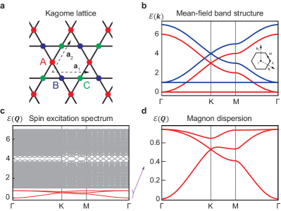
Figure 1: Spin excitation spectrum of kagome ferromagnet. (a) The kagome lattice. (b) The mean-field band structure for $N_{occ}=1$, $t=1$, $U=3$, and $\mu=-2$, where the lowest flat band in red is fully occupied. Red and blue lines represent the $\uparrow$ and $\downarrow$ spin bands, respectively. (c) The spin excitation spectrum. Red and grey lines correspond to the magnon bands and Stoner continuum, respectively. (d) The magnon band structure.

For illustration, let us describe the spin excitation spectrum of a saturated ferromagnet on the kagome lattice shown in Fig. 1 (a). The tight-binding Hamiltonian containing only the nearest-neighbor hopping amplitude $t>0$ is given by

$$h({\bm{k}})=2t\begin{pmatrix}0&\cos\frac{{\bm{k}}\cdot{\bm{a}}_{1}}{2}&\cos\frac{{\bm{k}}\cdot{\bm{a}}_{2}}{2}\\ \cos\frac{{\bm{k}}\cdot{\bm{a}}_{1}}{2}&0&\cos\frac{{\bm{k}}\cdot({\bm{a}}_{1}-{\bm{a}}_{2})}{2}\\ \cos\frac{{\bm{k}}\cdot{\bm{a}}_{2}}{2}&\cos\frac{{\bm{k}}\cdot({\bm{a}}_{1}-{\bm{a}}_{2})}{2}&0\end{pmatrix}-\mu{\mathbf{I}},$$ (7)

where ${\bm{a}}_{1}=(1,0)$ and ${\bm{a}}_{2}=(\frac{1}{2},\frac{\sqrt{3}}{2})$, $\mu$ is the chemical potential, and ${\mathbf{I}}$ is an identity matrix. This model has a spin-degenerate flat band at the bottom. At 0 K, this model exhibits saturated ferromagnetism at any $U>0$ when the bottom flat band is half filled, i.e., $N_{occ}=1$ and $v=1/6$ Mielke (1991, 1992). The corresponding spin-split mean-field band structure is shown in Fig. 1 (b). The relevant spin excitation spectrum in Fig. 1(c), composed of the Stoner continuum and spin wave excitations, is obtained by diagonalizing Eq. (6) at each ${\bm{Q}}$. In general, there are $N_{orb}$ magnons, which consists of $1$ gapless Goldstone mode and $N_{orb}-1$ gapped modes. When the ground state is ferromagnetic, the gapless magnon exhibits a quadratic dispersion with an energy minimum at ${\bm{Q}}={\bm{0}}$. Conversely, a negative (or zero) magnon energy indicates that the ferromagnetic ground state is unstable Kusakabe and Aoki (1994); Alavirad and Sau (2020).

Upper bound for spin stiffness.— Now let us assume a ferromagnetic ground state, and use perturbation theory to derive an upper bound of the spin stiffness:

$$D_{\mu\nu}\equiv\partial_{\mu}\partial_{\nu}\mathcal{E}_{m}({\bm{Q}})|_{{\bm{Q}}={\bm{0}}}.$$ (8)

Here, $\mathcal{E}_{m}({\bm{Q}})$ is the energy of the gapless magnon with momentum ${\bm{Q}}$. We reorganize Eq. (6) as $\mathcal{H}^{SE}({\bm{Q}})=\mathcal{H}^{SE}({\bm{0}})+V({\bm{Q}})$ and treat $V({\bm{Q}})\equiv\mathcal{H}^{SE}({\bm{Q}})-\mathcal{H}^{SE}({\bm{0}})$ as the $U$ independent perturbation.

Eq. (5) is exactly solved at ${\bm{Q}}=0$ with $z_{{\bm{k}}^{\prime}\beta n^{\prime}}({\bm{0}})=|u_{n^{\prime}}({\bm{k}}^{\prime})\rangle_{\beta}$ and $\mathcal{E}({\bm{0}})=0$. The assumption of ferromagnetism prohibits $\mathcal{E}({\bm{0}})<0$, and thus $\mathcal{E}_{m}({\bm{0}})=0$ becomes the ground state energy of the unperturbed Hamiltonian $\mathcal{H}^{SE}({\bm{0}})$. The magnon energy up to first order perturbation is therefore:

$$\mathcal{E}_{m}^{(1)}({\bm{Q}})=\frac{\langle z^{GS}({\bm{0}})|V({\bm{Q}})|z^{GS}({\bm{0}})\rangle}{\langle z^{GS}({\bm{0}})|z^{GS}({\bm{0}})\rangle},$$ (9)

where $|z^{GS}({\bm{0}})\rangle$ is the ground state of $\mathcal{H}^{SE}({\bm{0}})$.

Since first order perturbation uses the ground state of the unperturbed Hamiltonian to calculate the energy of the perturbed Hamiltonian, it overestimates the true ground state energy in general (see SM for details). Together with the fact that $\mathcal{E}_{m}({\bm{Q}})$ increases with $U$, we obtain the following inequality,

$$\mathcal{E}_{m}({\bm{Q}})|_{U<\infty}\leq\mathcal{E}_{m}({\bm{Q}})|_{U\rightarrow\infty}\leq\mathcal{E}_{m}^{(1)}({\bm{Q}}).$$ (10)

Utilizing that both inequalities saturate at ${\bm{Q}}={\bm{0}}$, we can convert Eq. (10) to the inequality on spin stiffness as

$$D_{\mu\mu}(U<\infty)\leq D_{\mu\mu}(U\rightarrow\infty)\leq D^{(1)}_{\mu\mu},$$ (11)

where $D_{\mu\nu}^{(1)}\equiv\partial_{\mu}\partial_{\nu}\mathcal{E}_{m}^{(1)}({\bm{Q}})|_{{\bm{Q}}={\bm{0}}}$ is the first order spin stiffness (see SM for details).

In Fig. 2, we demonstrate the validity of Eq. (11) in the kagome lattice. Interestingly, the second inequality of Eq. (11) saturates in Fig. 2 (b), which is also true for a number of other lattice models. In such cases, the strongly correlated limit is governed solely by the energy and quantum geometry of the single particle Hamiltonian, as we shortly show.

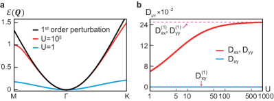
Figure 2: Upper bound for the spin stiffness of the kagome saturated ferromagnet. (a) The gapless magnon dispersion. Red and blue lines correspond to $U=10^{5}$ and $U=1$ cases, respectively. The black curve indicates the upper bound $\mathcal{E}_{m}^{(1)}({\bm{Q}})$. (b) Spin stiffness as a function of $U$. Due to $C_{3z}$ symmetry, $D_{xx}=D_{yy}$ and $D_{xy}=0$. The red and blue curves correspond to $D_{xx}(D_{yy})$ and $D_{xy}$, respectively. The purple dashed lines are the upper bounds $D^{(1)}_{\mu\mu}$, which are identical to the spin stiffness at $U\rightarrow\infty$.

To describe the gapless magnon dispersion near the $\Gamma$ point, we expand $\mathcal{E}_{m}^{(1)}({\bm{Q}})$ in powers of $Q_{\mu}$ up to quadratic order to obtain

$$\mathcal{E}_{m}^{(1)}({\bm{Q}}) =\frac{Q_{\mu}Q_{\nu}}{2N_{c}N_{occ}}\sum_{{\bm{k}}}^{N_{c}}[\sum_{n}^{N_{occ}}\partial_{\mu}\partial_{\nu}E_{n}({\bm{k}})+$$

$$2\sum_{m>N_{occ}}^{N_{orb}}\sum_{n}^{N_{occ}}(E_{m}({\bm{k}})-E_{n}({\bm{k}}))\chi_{\mu\nu}^{mn}({\bm{k}})],$$ (12)

where a summation over the $\mu$ and $\nu$ indices is assumed (see SM for details). Here, $\chi_{\mu\nu}^{mn}({\bm{k}})$ is the fidelity tensor defined as $\chi_{\mu\nu}^{mn}({\bm{k}})\equiv\langle\partial_{\mu}u_{m}({\bm{k}})|u_{n}({\bm{k}})\rangle\langle u_{n}({\bm{k}})|\partial_{\nu}u_{m}({\bm{k}})\rangle$, which characterizes the transition probability between the $m$-th and $n$-th band Jozsa (1994); Hwang et al. (2021). Eq. (12) explicitly shows that $\mathcal{E}_{m}^{(1)}({\bm{Q}})$ is composed of two separate terms. One is the sum of the electronic band curvature and the other is the sum of the transition probabilities between the unoccupied and occupied bands weighted by their energy difference. Note that by unoccupied bands, we refer to the $(N_{orb}-N_{occ})$ unoccupied $\uparrow$-spin bands of $h({\bm{k}})$.

No-go theorem.— Using Eqs. (10), (11), and (12), we derive a no-go theorem that forbids saturated ferromagnetism. Explicitly, we show that for systems described by a repulsive Hubbard model, if the spin-polarized occupied bands are either isolated or flat, saturated ferromagnetism is forbidden when the fidelity between the occupied and unoccupied bands is zero. Also, as a corollary, we prove the absence of saturated ferromagnetism in any half-filled Hubbard model. Since $D_{\mu\nu}$ is a positive definite tensor for a ferromagnetic ground state, one can derive the no-go theorem by examining the condition for $D_{\mu\nu}^{(1)}=0$.

Let us consider the band structure of $\uparrow$-spin electrons described by $h({\bm{k}})$. If the occupied bands are separated from the unoccupied bands by a direct gap, the first term of Eq. (12) is zero, since $E_{n}({\bm{k}})$ are smooth and periodic in the Brillouin zone. Likewise, if the occupied bands are flat, the same term vanishes as well, even when band crossings with the unoccupied bands exist. In such cases, if we further assume no interband coupling between the occupied and unoccupied bands, i.e., $\chi_{\mu\nu}^{mn}({\bm{k}})=0$, the second term also vanishes, which completes the proof of the no-go theorem.

Specifically, in the case of the half-filled Hubbard model with $N_{occ}=N_{orb}$, saturated ferromagnetism indicates that all $\uparrow$-spin bands are fully occupied. Without any unoccupied bands, $\chi_{\mu\nu}^{mn}({\bm{k}})$ should be zero by definition. Since the first term of Eq. (12) also vanishes due to the periodicity and smoothness of the energy bands, we find that saturated ferromagnetism is strictly forbidden in any half-filled repulsive Hubbard model in arbitrary dimension. A particularly important consequence is that any repulsive Hubbard model with a single orbital cannot exhibit saturated ferromagnetism at integer filling. We demonstrate the no-go theorem by examining the magnon dispersion of several half-filled Hubbard models in the SM.

Relation to quantum geometry.— Let us discuss the geometric meaning of the upper bound in Eq. (12). In general, the geometry of the quantum state $|u_{n}({\bm{k}})\rangle$ is characterzied by the quantum geometric tensor (QGT) $\mathfrak{G}_{ij}^{n}({\bm{k}})$ whose real and imaginary parts correspond to the quantum metric and Berry curvature, respectively. Explicitly,

$$\mathfrak{G}_{\mu\nu}^{n}({\bm{k}}) =\langle\partial_{\mu}u_{n}({\bm{k}})|[{{\mathbf{I}}}-P_{n}({\bm{k}})]|\partial_{\nu}u_{n}({\bm{k}})\rangle$$

$$=\sum_{m\neq n}\langle\partial_{\mu}u_{n}({\bm{k}})|u_{m}({\bm{k}})\rangle\langle u_{m}({\bm{k}})|\partial_{\nu}u_{n}({\bm{k}})\rangle$$

$$=\sum_{m\neq n}\chi_{\mu\nu}^{nm}({\bm{k}}),$$ (13)

where the projector $P_{n}({\bm{k}})$ is defined as $P_{n}({\bm{k}})=|u_{n}({\bm{k}})\rangle\langle u_{n}({\bm{k}})|$. This shows that the QGT $\mathfrak{G}_{\mu\nu}^{n}({\bm{k}})$ of the $n$-th band is given by the summation of the fidelity tensor $\chi_{\mu\nu}^{nm}({\bm{k}})$ over all $m\neq n$. In multiband cases, the Abelian QGT can be generalized as Hwang et al. (2021)

$$\mathfrak{G}_{\mu\nu}({\bm{k}}) \equiv\sum_{n=1}^{N_{occ}}\langle\partial_{\mu}u_{n}({\bm{k}})|[{\mathbf{I}}-P_{occ}({\bm{k}})]|\partial_{\nu}u_{n}({\bm{k}})\rangle$$

$$=\sum_{m>N_{occ}}^{N_{orb}}\sum_{n}^{N_{occ}}\chi_{\mu\nu}^{nm}({\bm{k}}),$$ (14)

where $P_{occ}({\bm{k}})=\sum_{n=1}^{N_{occ}}|u_{n}({\bm{k}})\rangle\langle u_{n}({\bm{k}})|$. The similarity between Eq. (12) and Eq. (14) indicates the geometric character of the spin stiffness.

In particular, when the occupied and unoccupied bands are fully degenerate among themselves, $\Delta({\bm{k}})\equiv E_{m}({\bm{k}})-E_{n}({\bm{k}})$ is independent of $m$ and $n$, which leads to

$$\mathcal{E}_{m}^{(1)}({\bm{Q}})=\frac{Q_{\mu}Q_{\nu}}{2N_{c}N_{occ}}\sum_{{\bm{k}}}^{N_{c}}[\sum_{n}^{N_{occ}}\partial_{\mu}\partial_{\nu}E_{n}({\bm{k}})+2\Delta({\bm{k}})g_{\mu\nu}({\bm{k}})],$$ (15)

where $g_{\mu\nu}({\bm{k}})=(\mathfrak{G}_{\mu\nu}({\bm{k}})+\mathfrak{G}_{\nu\mu}({\bm{k}}))/2$ is the Abelian quantum metric. This directly follows from Eq. (14), $\chi_{\mu\nu}^{mn}({\bm{k}})=\chi_{\nu\mu}^{nm}({\bm{k}})$, and the fact that $D_{\mu\nu}$ is a symmetric tensor. We note that Eq. (15) always holds for two-orbital models with 1 occupied and 1 unoccupied band, which indicates that in such systems, a non-vanishing quantum metric is essential for the emergence of saturated ferromagnetism.

To demonstrate the effect of the quantum metric on spin stiffness, we compare the gapless magnon spectra of two models with identical electronic band structure but different quantum metrics. Explicitly, let us consider a system in the wallpaper group $p3$ as in Fig. 3(a), and place three orbitals whose $C_{3z}$ eigenvalues are $1$, $\omega$, and $\omega^{2}$ ($\omega=e^{\frac{2\pi i}{3}}$), respectively, at the $1a$ Wyckoff position. Here, $C_{3z}$ indicates a 3-fold rotation about the $z$-axis. We consider one occupied flat band at the Fermi level ($E=0$) and two degenerate unoccupied bands with energy $E_{unocc}({\bm{k}})=3+\cos{\bm{k}}\cdot{\bm{a}}_{1}+\cos{\bm{k}}\cdot{\bm{a}}_{2}+\cos{\bm{k}}\cdot({\bm{a}}_{1}-{\bm{a}}_{2})$. The relevant Hamiltonian is given by

$$h({\bm{k}})=E_{unocc}({\bm{k}})({\mathbf{I}}-P({\bm{k}})),$$ (16)

where $P({\bm{k}})=|u_{1}({\bm{k}})\rangle\langle u_{1}({\bm{k}})|$ is the occupied band projector. The corresponding electronic energy spectrum is shown in Fig. 3(b).

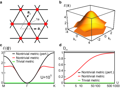
Figure 3: Influence of the quantum metric on the spin stiffness. (a) Lattice structure belonging to wallpaper group $p3$. ${\bm{a}}_{1}=(1,0)$ and ${\bm{a}}_{2}=(\frac{1}{2},\frac{\sqrt{3}}{2})$ are the primitive lattice vectors. (b) The band structure of the Hamiltonian in Eq. (16). The system consists of a single occupied flat band at $E=0$, which is separated from two degenerate dispersive bands. (c) Gapless magnon spectrum for $U=10^{5}$. (d) $D_{xx}$ plotted as a function of $U$. In this model, $D_{xx}=D_{yy}$ and $D_{xy}=0$ due to $C_{3z}$ symmetry. We note that $D_{\mu\nu}(U\rightarrow\infty)=D_{\mu\nu}^{(1)}$. In (c) and (d), the red and black curves are numerical data and the upper bound, respectively, for the model with nontrivial quantum metric. The green curves are calculated for the case with zero quantum metric.

In this model, the Abelian quantum metric of the occupied band is expressed as Herzog-Arbeitman et al. (2022)

$$g_{\mu\nu}({\bm{k}})=\frac{1}{2}Tr\partial_{\mu}P({\bm{k}})\partial_{\nu}P({\bm{k}}),$$ (17)

where the trace is performed on the orbital indices. Thus, we can tune $g_{\mu\nu}({\bm{k}})$ by changing $P({\bm{k}})$ or $|u_{1}({\bm{k}})\rangle.$ The trivial model with zero quantum metric is constructed by using $|u_{1}({\bm{k}})\rangle=(1,0,0)^{T}$. Following Ref. Herzog-Arbeitman et al. (2022), we construct the nontrivial model with

$$|u_{1}({\bm{k}})\rangle=\frac{1}{3}\begin{pmatrix}1+e^{-i{\bm{k}}\cdot{\bm{a}}_{1}}+e^{-i{\bm{k}}\cdot{\bm{a}}_{2}}\\ 1+\omega e^{-i{\bm{k}}\cdot{\bm{a}}_{1}}+\omega^{2}e^{-i{\bm{k}}\cdot{\bm{a}}_{2}}\\ 1+\omega^{2}e^{-i{\bm{k}}\cdot{\bm{a}}_{1}}+\omega e^{-i{\bm{k}}\cdot{\bm{a}}_{2}}\end{pmatrix},$$ (18)

whose quantum metric is $g_{\mu\nu}({\bm{k}})=\delta_{\mu\nu}/6$ in orthogonal coordinates. From Eq. (15), we obtain $D_{\mu\nu}^{(1)}=0$ and $\delta_{\mu\nu}$ for the trivial and nontrivial models, respectively. Fig. 3(c) and (d) show the calculation of the gapless magnon spectrum and spin stiffness. The two models show drastically different behavior despite the same energy dispersion, which demonstrates the significance of quantum metric on the computed quantities. Moreover, the quantum metric solely controls the model’s capability to host saturated ferromagnetism.

Lastly, when $\Delta({\bm{k}})=\Delta$ is independent of ${\bm{k}}$ in an insulator, Eq. (15) reduces to a simpler relation to the Abelian quantum metric:

$$D_{\mu\nu}^{(1)}=\frac{2\Delta}{N_{c}N_{occ}}\sum_{{\bm{k}}}^{N_{c}}g_{\mu\nu}({\bm{k}}).$$ (19)

In such cases, the lower bounds of the quantum metric proposed in previous studies can be used to impose topological constraint on $D_{\mu\nu}^{(1)}$. For instance, the well-known inequality between the trace of the quantum metric and the Berry curvature Peotta and Törmä (2015); Xie et al. (2020) gives a lower bound of the spin stiffness imposed by the Chern number of occupied bands, indicating that the band topology may stabilize saturated ferromagnetism. Similarly, the fragile or obstructed atomic band topology can also give another lower bound that can be obtained from real space invariants developed recently Herzog-Arbeitman et al. (2022); Song et al. (2020) (See SM).

Discussion.— We have shown that quantum geometry plays an essential role in stabilizing saturated ferromagnetism, relevant to ferromagnetic insulators or semimetals McGuire et al. (2015); Song et al. (2006); Meng et al. (2018); Zhang et al. (2016); Liu et al. (2018); Kim et al. (2018); Jin et al. (2017); Liu et al. (2019). This implies that ferromagnetic insulators or semimetals can be realized in materials which intrinsically have strong interband couplings. This may be the physical reason why most ferromagnets found in nature are metals; for an insulator to be a ferromagnet, a nontrivial quantum geometry is required. We emphasize that the validity of these results is mathematically rigorous beyond mean-field theory (See SM). Although our theory is limited to saturated ferromagnetism, considering that rigorous statements about the stability of general ferromagnetism are either very rare or relying on the restricted forms of the kinetic Hamiltonian Tasaki (2020), we believe that our work provides a significant insight for understanding the fundamental origin of ferromagnetism and its relation to the quantum geometry. Extending our theory to general broken symmetry ground states in itinerant electronic systems would be one important direction for future study.

Supplemental Material for “ Quantum geometric bound for saturated ferromagnetism ”

S1 Tight-binding conventions

In this Appendix, we establish the tight-binding conventions used throughout this letter. We consider a $d$-dimensional periodic lattice spanned by the primitive lattice vectors $\{{\bm{a}}_{1},\dots,{\bm{a}}_{d}\}$. The tight-binding Hilbert space is spanned by Löwdin orbitals $c^{\dagger}_{i\alpha\sigma}$ labeled by the unit cell ${\bm{R}}_{i}$ ($i=1,\dots,N_{c}$), orbital ($\alpha=1,\dots,N_{orb}$), and spin ($\sigma=\uparrow,\downarrow$) indices. The momentum space basis is given by

$$c^{\dagger}_{{\bm{k}}\alpha\sigma}=\frac{1}{\sqrt{N_{c}}}\sum_{i}e^{i{\bm{k}}\cdot({\bm{R}}_{i}+{\bm{\tau}}_{\alpha})}c^{\dagger}_{i\alpha\sigma}.$$ (S1)

The tight-binding Hamiltonian can then be expressed as

$$H =H_{kin}+H_{int}$$

$$=\sum_{ij\alpha\beta\sigma}t_{ij}^{\alpha\beta}c^{\dagger}_{i\alpha\sigma}c_{j\beta\sigma}+U\sum_{i\alpha}c^{\dagger}_{i\alpha\uparrow}c^{\dagger}_{i\alpha\downarrow}c_{i\alpha\downarrow}c_{i\alpha\uparrow}$$

$$=\sum_{{\bm{k}}\alpha\beta\sigma}h({\bm{k}})_{\alpha\beta}c^{\dagger}_{{\bm{k}}\alpha\sigma}c_{{\bm{k}}\beta\sigma}+\frac{U}{N_{c}}\sum_{{\bm{k}}{\bm{k}}^{\prime}{\bm{q}}\alpha}c^{\dagger}_{{\bm{k}}+{\bm{q}}\alpha\uparrow}c^{\dagger}_{{\bm{k}}^{\prime}-{\bm{q}}\alpha\downarrow}c_{{\bm{k}}^{\prime}\alpha\downarrow}c_{{\bm{k}}\alpha\uparrow},$$ (S2)

where we neglect Umklapp scattering of the repulsive Hubbard interaction ($U>0$). We denote the eigenstates of the kinetic (noninteracting) Hamiltonian $h({\bm{k}})_{\alpha\beta}=\sum_{i}e^{-i{\bm{k}}\cdot({\bm{R}}_{i}+{\bm{\tau}}_{\alpha}-{\bm{\tau}}_{\beta})}t_{i0}^{\alpha\beta}$ by

$$h({\bm{k}})|u_{n}({\bm{k}})\rangle=E_{n}({\bm{k}})|u_{n}({\bm{k}})\rangle$$ (S3)

($n=1,\dots,N_{orb}$), where $|u_{n}({\bm{k}})\rangle$ is an $N_{orb}\times 1$ vector. In addition, we define the filling $v\equiv N_{occ}/2N_{orb}$, where $N_{occ}\in\mathbb{Z}$ electrons exist per unit cell, resulting in a total of $N_{tot}=N_{c}N_{occ}$ electrons. Note that we restrict the problem to cases where the band filling is an integer, which corresponds to an insulator or a semimetal where the band inversion occurs at the Fermi level.

S2 Mean-field Hamiltonian of saturated ferromagnets

In this Appendix, we review the mean-field properties of a ferromagnet. Following the main text, we assume that every occupied state has spin $\uparrow$. The mean-field Hamiltonian obtained by decoupling the many-body terms of the second line of Eq. (S2) is given by

$$H_{mf}=\sum_{{\bm{k}}\alpha\beta\sigma}h({\bm{k}})_{\alpha\beta}c^{\dagger}_{{\bm{k}}\alpha\sigma}c_{{\bm{k}}\beta\sigma}+U\sum_{{\bm{k}}\alpha\sigma}\langle n_{\alpha-\sigma}\rangle c^{\dagger}_{{\bm{k}}\alpha\sigma}c_{{\bm{k}}\alpha\sigma}-UN_{c}\sum_{\alpha}n_{\alpha\uparrow}n_{\alpha\downarrow},$$ (S4)

where $\langle n_{\alpha\sigma}\rangle=\langle c^{\dagger}_{i\alpha\sigma}c_{i\alpha\sigma}\rangle$ is the unit cell-independent orbital filling. In the $(\uparrow,\downarrow)^{T}\otimes(\alpha_{1},\dots,\alpha_{N_{orb}})^{T}$ basis, $H_{mf}({\bm{k}})$ is a $(2N_{orb}\times 2N_{orb})$ Hermitian matrix given by

$$H_{mf}({\bm{k}})=\begin{pmatrix}H_{\uparrow\uparrow}({\bm{k}})&H_{\uparrow\downarrow}({\bm{k}})\\ H_{\downarrow\uparrow}({\bm{k}})&H_{\downarrow\downarrow}({\bm{k}})\\ \end{pmatrix}=\begin{pmatrix}h({\bm{k}})&0\\ 0&h({\bm{k}})\\ \end{pmatrix}+U\begin{pmatrix}diag({\bm{n}}_{\downarrow})&0\\ 0&diag({\bm{n}}_{\uparrow})\\ \end{pmatrix},$$ (S5)

where ${\bm{n}}_{\sigma}=(n_{1\sigma},\dots,n_{N_{orb}\sigma})$. Since the $\downarrow$ bands are empty (${\bm{n}}_{\downarrow}={\bm{0}}$), the Hamiltonian of occupied states (which have $\uparrow$) is identical to $h({\bm{k}})$. This observation underscores that the ground state of a saturated ferromagnet is fully determined by the noninteracting Hamiltonian. As an example, we present the mean-field band structure of a kagome ferromagnet in Fig. 1(b) of the main text.

S3 Derivation of the spin excitation Hamiltonian

In this Appendix, we present a detailed derivation of the spin excitation Hamiltonian $\mathcal{H}^{SE}\equiv\mathcal{H}^{SE}_{{\bm{k}}\alpha n,{\bm{k}}^{\prime}\beta n^{\prime}}({\bm{Q}})$ in Eq. (6). $\mathcal{H}^{SE}$ is a Hermitian matrix, which is an effective Hamiltonian in the sense that it gives the spin excitation spectrum upon diagonalization. Let us define the fundamental variables under consideration. The momentum of spin excitation is denoted as ${\bm{Q}}$, its energy as $\mathcal{E}({\bm{Q}})$, and the gapless magnon energy as $\mathcal{E}_{m}({\bm{Q}})$. Following Eq. (S3), we begin by defining the occupied band electron creation operator as

$$\phi^{\dagger}_{n{\bm{k}}}=\sum_{\alpha}^{N_{orb}}c^{\dagger}_{{\bm{k}}\alpha\uparrow}|u_{n}({\bm{k}})\rangle_{\alpha},$$ (S6)

where $n\in\{1,\dots,N_{occ}\}$. The ground state is given by

$$|\Omega\rangle=\prod_{n}^{N_{occ}}\prod_{{\bm{k}}}^{N_{c}}\phi^{\dagger}_{n{\bm{k}}}|0\rangle,$$ (S7)

where $|0\rangle$ indicates the vacuum state. Consequently, spin excitations $|{\bm{Q}}\rangle$ with momentum ${\bm{Q}}$ are created by acting on $|\Omega\rangle$

$$\Psi_{{\bm{Q}}}^{\dagger}=\sum_{{\bm{k}}}^{N_{c}}\sum_{\alpha}^{N_{orb}}\sum_{n}^{N_{occ}}z_{{\bm{k}}\alpha n}({\bm{Q}})c^{\dagger}_{{\bm{k}}+{\bm{Q}}\alpha\downarrow}\phi_{n{\bm{k}}}.$$ (S8)

This describes a transition from occupied bands to spin $\downarrow$ orbitals, where $z_{{\bm{k}}\alpha n}({\bm{Q}})$ are arbitrary complex numbers to be determined.

The spin excitations are obtained by forming a proper choice of $z_{{\bm{k}}\alpha n}({\bm{Q}})$. Although it seems natural to solve for

$$H|{\bm{Q}}\rangle=(\mathcal{E}({\bm{Q}})+E_{GS})|{\bm{Q}}\rangle,$$ (S9)

an exact solution to it does not exist Sólyom (2010). To see this, note that the left hand side contains 2- and 3-body terms, while the right hand side contains a 1-body term. To satisfy the equality, one has to reduce the many body terms to a 1-body term using anticommutation relations and the ground state properties. However, direct calculation shows that $H_{int}|{\bm{Q}}\rangle$ cannot be simplified into a 1-body operator unless the system is half-filled; that is, the spin excitation spectrum is exactly solvable only at half filling. As a resolution, we define the spin excitations through a two-step approach: performing a mean-field decoupling of

$$\mathcal{E}({\bm{Q}})=\frac{\langle{\bm{Q}}|H|{\bm{Q}}\rangle}{\langle{\bm{Q}}|{\bm{Q}}\rangle}-\langle\Omega|H|\Omega\rangle,$$ (S10)

and employing a variational method with respect to $z^{*}_{{\bm{k}}\alpha n}({\bm{Q}})$. We demonstrate shortly after that this yields $\mathcal{H}^{SE}_{{\bm{k}}\alpha n,{\bm{k}}^{\prime}\beta n^{\prime}}({\bm{Q}})$.

We emphasize that the utilization of mean-field theory is not a mere approximation, but rather mathematically rigorous, as elaborated in the main text. Furthermore, it is worth mentioning that Eq. (S10) must be calculated using $H$ instead of $H_{mf}$. This is because a Goldstone mode appears when a continuous symmetry of the effective action, in our case the Hamiltonian, does not exist in the ground state. However, since $H_{mf}$ is obtained after spontaneous symmetry breaking, the $SU(2)$ symmetry is already broken in the Hamiltonian level. As a result, the spin excitation spectrum obtained from $H_{mf}$ is gapped.

Let us present the mean-field decoupling of Eq. (S10). To do so, we make use of the following identities,

$$\langle\phi^{\dagger}_{n_{1}{\bm{k}}_{1}}\phi_{n_{2}{\bm{k}}_{2}}\rangle=\delta_{n_{1}n_{2}}\delta_{{\bm{k}}_{1}{\bm{k}}_{2}},\quad(n_{i}\in[1,N_{occ}])$$

$$\langle c_{{\bm{k}}_{1}\alpha_{1}\downarrow}c^{\dagger}_{{\bm{k}}_{2}\alpha_{2}\downarrow}\rangle=\delta_{\alpha_{1}\alpha_{2}}\delta_{{\bm{k}}_{1}{\bm{k}}_{2}}$$

$$\langle c^{\dagger}_{{\bm{k}}\alpha\uparrow}c_{{\bm{k}}^{\prime}\beta\uparrow}\rangle=\delta_{{\bm{k}}{\bm{k}}^{\prime}}\sum_{n}^{N_{occ}}{}_{\alpha}\langle u_{n}({\bm{k}})|u_{n}({\bm{k}})\rangle_{\beta}.$$ (S11)

The third identity is obtained from

$$\sum_{n}^{N_{orb}}{}_{\beta}\langle u_{n}({\bm{k}})|\phi^{\dagger}_{n{\bm{k}}}=\sum_{n\alpha}^{N_{orb}}{}_{\beta}\langle u_{n}({\bm{k}})|u_{n}({\bm{k}})\rangle_{\alpha}c^{\dagger}_{{\bm{k}}\alpha\uparrow}=\sum_{\alpha}^{N_{orb}}\delta_{\alpha\beta}c^{\dagger}_{{\bm{k}}\alpha\uparrow}=c^{\dagger}_{{\bm{k}}\beta\uparrow}.$$ (S12)

It is worth noting that this is different from $\delta_{{\bm{k}}{\bm{k}}^{\prime}}\delta_{\alpha\beta}$, since the sum runs over $(1,\dots,N_{occ})$. From now on, we assume $\sum_{\alpha}=\sum_{\alpha}^{N_{orb}}$ and $\sum_{n}=\sum_{n}^{N_{occ}}$ for any orbital and band indices, unless specified otherwise.

Let $\langle{\bm{Q}}|H|{\bm{Q}}\rangle=I_{1}+I_{2}+I_{3}$, where $I_{1,2}=\langle{\bm{Q}}|\sum_{{\bm{k}}\alpha\beta}h({\bm{k}})_{\alpha\beta}c^{\dagger}_{{\bm{k}}\alpha\uparrow,\downarrow}c_{{\bm{k}}\alpha\uparrow,\downarrow}|{\bm{Q}}\rangle$ and $I_{3}=\langle{\bm{Q}}|H_{int}|{\bm{Q}}\rangle$. Denoting $\langle\dots\rangle=\langle\Omega|\dots|\Omega\rangle$, we obtain

$$I_{1} =\sum_{{\bm{k}}\alpha\beta}\langle{\bm{Q}}|h({\bm{k}})_{\alpha\beta}c^{\dagger}_{{\bm{k}}\alpha\uparrow}c_{{\bm{k}}\beta\uparrow}|{\bm{Q}}\rangle$$

$$=\sum_{{\bm{k}}\alpha\beta}\sum_{n_{1}\alpha_{1}{\bm{k}}_{1}}\sum_{n_{2}\alpha_{2}{\bm{k}}_{2}}z_{n_{1}\alpha_{1}{\bm{k}}_{1}}^{*}({\bm{Q}})z_{n_{2}\alpha_{2}{\bm{k}}_{2}}({\bm{Q}})h({\bm{k}})_{\alpha\beta}\langle\phi^{\dagger}_{n_{1}{\bm{k}}_{1}}c_{{\bm{k}}_{1}+{\bm{Q}}\alpha_{1}\downarrow}c^{\dagger}_{{\bm{k}}\alpha\uparrow}c_{{\bm{k}}\beta\uparrow}c^{\dagger}_{{\bm{k}}_{2}+{\bm{Q}}\alpha_{2}\downarrow}\phi_{n_{2}{\bm{k}}_{2}}\rangle.$$ (S13)

We apply mean-field decoupling to $\langle\dots\rangle$ and decompose it into a product of 1-body correlations. Upon doing so, two nonzero contractions survive, which we denote as $\langle\dots\rangle=I_{1}^{\prime}+I_{1}^{\prime\prime}$. The first term

$$I_{1}^{\prime} =-\langle\phi^{\dagger}_{n_{1}{\bm{k}}_{1}}c_{{\bm{k}}\beta\uparrow}\rangle\langle c_{{\bm{k}}_{1}+{\bm{Q}}\alpha_{1}\downarrow}c^{\dagger}_{{\bm{k}}_{2}+{\bm{Q}}\alpha_{2}\downarrow}\rangle\langle c^{\dagger}_{{\bm{k}}\alpha\uparrow}\phi_{n_{2}{\bm{k}}_{2}}\rangle$$

$$=-\delta_{{\bm{k}}_{1}{\bm{k}}}\delta_{{\bm{k}}_{1}{\bm{k}}_{2}}\sum_{\alpha_{3}\alpha_{4}}{}_{\alpha_{4}}\langle u_{n_{2}}({\bm{k}}_{2})|u_{n_{1}}({\bm{k}}_{1})\rangle_{\alpha_{3}}\langle c^{\dagger}_{{\bm{k}}_{1}\alpha_{3}\uparrow}c_{{\bm{k}}\beta\uparrow}\rangle\langle c^{\dagger}_{{\bm{k}}\alpha\uparrow}c_{{\bm{k}}\alpha_{4}\uparrow}\rangle$$

$$=-\delta_{{\bm{k}}_{1}{\bm{k}}}\delta_{{\bm{k}}_{1}{\bm{k}}_{2}}\sum_{\alpha_{3}\alpha_{4}}\sum_{n_{3}n_{4}}{}_{\alpha_{4}}\langle u_{n_{2}}({\bm{k}})|u_{n_{1}}({\bm{k}})\rangle_{\alpha_{3}}{}_{\alpha_{3}}\langle u_{n_{3}}({\bm{k}})|u_{n_{3}}({\bm{k}})\rangle_{\beta}{}_{\alpha}\langle u_{n_{4}}({\bm{k}})|u_{n_{4}}({\bm{k}})\rangle_{\alpha_{4}}$$

$$=-\delta_{{\bm{k}}_{1}{\bm{k}}}\delta_{{\bm{k}}_{1}{\bm{k}}_{2}}\sum_{\alpha_{3}\alpha_{4}}\sum_{n_{3}n_{4}}{}_{\alpha_{4}}\langle u_{n_{2}}({\bm{k}})|u_{n_{4}}({\bm{k}})\rangle_{\alpha_{4}}{}_{\alpha_{3}}\langle u_{n_{3}}({\bm{k}})|u_{n_{1}}({\bm{k}})\rangle_{\alpha_{3}}{}_{\alpha}\langle u_{n_{4}}({\bm{k}})|u_{n_{3}}({\bm{k}})\rangle_{\beta}$$

$$=-\delta_{{\bm{k}}_{1}{\bm{k}}}\delta_{{\bm{k}}_{1}{\bm{k}}_{2}}{}_{\alpha}\langle u_{n_{2}}({\bm{k}})|u_{n_{1}}({\bm{k}})\rangle_{\beta}$$ (S14)

upon summation yields

$$-\sum_{n_{1}n_{2}\alpha_{1}{\bm{k}}\alpha\beta}z^{*}_{n_{1}\alpha_{1}{\bm{k}}}({\bm{Q}})z_{n_{2}\alpha_{1}{\bm{k}}}({\bm{Q}})h({\bm{k}})_{\alpha\beta}{}_{\alpha}\langle u_{n_{2}}({\bm{k}})|u_{n_{1}}({\bm{k}})\rangle_{\beta}=-\sum_{n\alpha{\bm{k}}}|z_{n\alpha{\bm{k}}}({\bm{Q}})|^{2}E_{n}({\bm{k}}).$$ (S15)

The second term is given by

$$I_{1}^{\prime\prime} =\langle\phi^{\dagger}_{n_{1}{\bm{k}}_{1}}\phi_{n_{2}{\bm{k}}_{2}}\rangle\langle c_{{\bm{k}}_{1}+{\bm{Q}}\alpha_{1}\downarrow}c^{\dagger}_{{\bm{k}}_{2}+{\bm{Q}}\alpha_{2}\downarrow}\rangle\langle c^{\dagger}_{{\bm{k}}\alpha\uparrow}c_{{\bm{k}}\beta\uparrow}\rangle$$

$$=\sum_{n_{3}}^{N_{occ}}{}_{\alpha}\langle u_{n_{3}}({\bm{k}})|u_{n_{3}}({\bm{k}})\rangle_{\beta}\delta_{n_{1}n_{2}}\delta_{\alpha_{1}\alpha_{2}}\delta_{{\bm{k}}_{1}{\bm{k}}_{2}},$$ (S16)

which evaluates to

$$\sum_{n_{1}\alpha_{1}{\bm{k}}_{1}{\bm{k}}\alpha\beta}|z_{n_{1}\alpha_{1}k_{1}}({\bm{Q}})|^{2}\sum_{n_{3}}{}_{\alpha}\langle u_{n_{3}}({\bm{k}})|u_{n_{3}}({\bm{k}})\rangle_{\beta}h({\bm{k}})_{\alpha\beta}=\sum_{n\alpha{\bm{k}}}|z_{n\alpha{\bm{k}}}({\bm{Q}})|^{2}\sum_{n^{\prime}{\bm{k}}^{\prime}}E_{n^{\prime}}({\bm{k}}^{\prime}).$$ (S17)

Thus, $I_{1}=\sum_{n\alpha{\bm{k}}}|z_{n\alpha{\bm{k}}}({\bm{Q}})|^{2}\sum_{n^{\prime}{\bm{k}}^{\prime}}E_{n^{\prime}}({\bm{k}}^{\prime})-\sum_{n\alpha{\bm{k}}}|z_{n\alpha{\bm{k}}}({\bm{Q}})|^{2}E_{n}({\bm{k}})$.

Similarly, the second term results in

$$I_{2} =\sum_{{\bm{k}}\alpha\beta}h({\bm{k}})_{\alpha\beta}\langle{\bm{Q}}|c^{\dagger}_{{\bm{k}}\alpha\downarrow}c_{{\bm{k}}\beta\downarrow}|{\bm{Q}}\rangle$$

$$=\sum_{{\bm{k}}\alpha\beta}\sum_{n_{1}\alpha_{1}{\bm{k}}_{1}}\sum_{n_{2}\alpha_{2}{\bm{k}}_{2}}z_{n_{1}\alpha_{1}{\bm{k}}_{1}}^{*}({\bm{Q}})z_{n_{2}\alpha_{2}{\bm{k}}_{2}}({\bm{Q}})h({\bm{k}})_{\alpha\beta}\langle\phi^{\dagger}_{n_{1}{\bm{k}}_{1}}c_{{\bm{k}}_{1}+{\bm{Q}}\alpha_{1}\downarrow}c^{\dagger}_{{\bm{k}}\alpha\downarrow}c_{{\bm{k}}\beta\downarrow}c^{\dagger}_{{\bm{k}}_{2}+{\bm{Q}}\alpha_{2}\downarrow}\phi_{n_{2}{\bm{k}}_{2}}\rangle$$

$$=\sum_{n_{1}{\bm{k}}_{1}\alpha\beta}z^{*}_{n_{1}\alpha{\bm{k}}_{1}}({\bm{Q}})z_{n_{1}\beta{\bm{k}}_{1}}({\bm{Q}})h({\bm{k}}_{1}+{\bm{Q}})_{\alpha\beta},$$ (S18)

The third term is expressed as

$$I_{3} =\frac{U}{N_{c}}\sum_{{\bm{k}}{\bm{k}}^{\prime}{\bm{q}}\alpha}\langle{\bm{Q}}|c^{\dagger}_{{\bm{k}}+{\bm{q}}\alpha\uparrow}c^{\dagger}_{{\bm{k}}^{\prime}-{\bm{q}}\alpha\downarrow}c_{{\bm{k}}^{\prime}\alpha\downarrow}c_{{\bm{k}}\alpha\uparrow}|{\bm{Q}}\rangle$$

$$=\frac{U}{N_{c}}\sum_{n_{1}\alpha_{1}{\bm{k}}_{1}}\sum_{n_{2}\alpha_{2}{\bm{k}}_{2}}\sum_{{\bm{k}}{\bm{k}}^{\prime}{\bm{q}}\alpha}z_{n_{1}\alpha_{1}{\bm{k}}_{1}}^{*}({\bm{Q}})z_{n_{2}\alpha_{2}{\bm{k}}_{2}}({\bm{Q}})\langle\phi^{\dagger}_{n_{1}{\bm{k}}_{1}}c_{{\bm{k}}_{1}+{\bm{Q}}\alpha_{1}\downarrow}c^{\dagger}_{{\bm{k}}+{\bm{q}}\alpha\uparrow}c^{\dagger}_{{\bm{k}}^{\prime}-{\bm{q}}\alpha\downarrow}c_{{\bm{k}}^{\prime}\alpha\downarrow}c_{{\bm{k}}\alpha\uparrow}c^{\dagger}_{{\bm{k}}_{2}+{\bm{Q}}\alpha_{2}\downarrow}\phi_{n_{2}{\bm{k}}_{2}}\rangle.$$ (S19)

This contains two nonzero contractions. Again, we denote $\langle\dots\rangle=I_{3}^{\prime}+I_{3}^{\prime\prime}$, and calculate these terms. Upon doing so, the first term evaluates to

$$I_{3}^{\prime} =-\langle\phi^{\dagger}_{n_{1}{\bm{k}}_{1}}c_{{\bm{k}}\alpha\uparrow}\rangle\langle c^{\dagger}_{{\bm{k}}+{\bm{q}}\alpha\uparrow}\phi_{n_{2}{\bm{k}}_{2}}\rangle\langle c_{{\bm{k}}_{1}+{\bm{Q}}\alpha_{1}\downarrow}c^{\dagger}_{{\bm{k}}^{\prime}-{\bm{q}}\alpha\downarrow}\rangle\langle c_{{\bm{k}}^{\prime}\alpha\downarrow}c^{\dagger}_{{\bm{k}}_{2}+{\bm{Q}}\alpha_{2}\downarrow}\rangle$$

$$=-\sum_{\alpha_{3}\alpha_{4}}{}_{\alpha_{4}}\langle u_{n_{2}}({\bm{k}}_{2})|u_{n_{1}}({\bm{k}}_{1})\rangle_{\alpha_{3}}\langle c^{\dagger}_{{\bm{k}}_{1}\alpha_{3}\uparrow}c_{{\bm{k}}\alpha\uparrow}\rangle\langle c^{\dagger}_{{\bm{k}}+{\bm{q}}\alpha\uparrow}c_{{\bm{k}}_{2}\alpha_{4}\uparrow}\rangle\langle c_{{\bm{k}}_{1}+{\bm{Q}}\alpha_{1}\downarrow}c^{\dagger}_{{\bm{k}}^{\prime}-{\bm{q}}\alpha\downarrow}\rangle\langle c_{{\bm{k}}^{\prime}\alpha\downarrow}c^{\dagger}_{{\bm{k}}_{2}+{\bm{Q}}\alpha_{2}\downarrow}\rangle$$

$$=-\sum_{\alpha_{3}\alpha_{4}}\sum_{n_{3}n_{4}}{}_{\alpha_{4}}\langle u_{n_{2}}({\bm{k}}_{2})|u_{n_{1}}({\bm{k}}_{1})\rangle_{\alpha_{3}}{}_{\alpha_{3}}\langle u_{n_{3}}({\bm{k}})|u_{n_{3}}({\bm{k}})\rangle_{\alpha}{}_{\alpha}\langle u_{n_{4}}({\bm{k}}+{\bm{q}})|u_{n_{4}}({\bm{k}}+{\bm{q}})\rangle_{\alpha_{4}}$$

$$\quad\quad\quad\quad\quad\quad\quad\times\delta_{{\bm{k}}{\bm{k}}_{1}}\delta_{{\bm{k}}_{2},{\bm{k}}+{\bm{q}}}\delta_{{\bm{k}}_{1}+{\bm{Q}},{\bm{k}}^{\prime}-{\bm{q}}}\delta_{{\bm{k}}^{\prime},{\bm{k}}_{2}+{\bm{Q}}}\delta_{\alpha\alpha_{1}}\delta_{\alpha\alpha_{2}}$$

$$=-\sum_{\alpha_{3}\alpha_{4}}\sum_{n_{3}n_{4}}{}_{\alpha_{3}}\langle u_{n_{3}}({\bm{k}})|u_{n_{1}}({\bm{k}})\rangle_{\alpha_{3}}{}_{\alpha_{4}}\langle u_{n_{2}}({\bm{k}}+{\bm{q}})|u_{n_{4}}({\bm{k}}+{\bm{q}})\rangle_{\alpha_{4}}{}_{\alpha}\langle u_{n_{4}}({\bm{k}}+{\bm{q}})|u_{n_{3}}({\bm{k}})\rangle_{\alpha}$$

$$\quad\quad\quad\quad\quad\quad\quad\times\delta_{{\bm{k}}{\bm{k}}_{1}}\delta_{{\bm{k}}_{2},{\bm{k}}+{\bm{q}}}\delta_{{\bm{k}}^{\prime},{\bm{k}}+{\bm{q}}+{\bm{Q}}}\delta_{\alpha\alpha_{1}}\delta_{\alpha\alpha_{2}}$$

$$=-\sum_{n_{3}n_{4}}{}_{\alpha}\langle u_{n_{4}}({\bm{k}}+{\bm{q}})|u_{n_{3}}({\bm{k}})\rangle_{\alpha}\delta_{n_{1}n_{3}}\delta_{n_{2}n_{4}}\delta_{{\bm{k}}{\bm{k}}_{1}}\delta_{{\bm{k}}_{2},{\bm{k}}+{\bm{q}}}\delta_{{\bm{k}}^{\prime},{\bm{k}}+{\bm{q}}+{\bm{Q}}}\delta_{\alpha\alpha_{1}}\delta_{\alpha\alpha_{2}}$$

$$=-{}_{\alpha}\langle u_{n_{2}}({\bm{k}}+{\bm{q}})|u_{n_{1}}({\bm{k}})\rangle\delta_{{\bm{k}}{\bm{k}}_{1}}\delta_{{\bm{k}}_{2},{\bm{k}}+{\bm{q}}}\delta_{{\bm{k}}^{\prime},{\bm{k}}+{\bm{q}}+{\bm{Q}}}\delta_{\alpha\alpha_{1}}\delta_{\alpha\alpha_{2}},$$ (S20)

where $n_{3},n_{4}$ are summed over $1,\dots,N_{occ}$. As usual, the orbital indices are summed over $1,\dots,N_{orb}$. The second contraction is given by

$$I_{3}^{\prime\prime} =\langle\phi^{\dagger}_{n_{1}{\bm{k}}_{1}}\phi_{n_{2}{\bm{k}}_{2}}\rangle\langle c^{\dagger}_{{\bm{k}}+{\bm{q}}\alpha\uparrow}c_{{\bm{k}}\alpha\uparrow}\rangle\langle c_{{\bm{k}}_{1}+{\bm{Q}}\alpha_{1}\downarrow}c^{\dagger}_{{\bm{k}}^{\prime}-{\bm{q}}\alpha\downarrow}\rangle\langle c_{{\bm{k}}^{\prime}\alpha\downarrow}c^{\dagger}_{{\bm{k}}_{2}+{\bm{Q}}\alpha_{2}\downarrow}\rangle$$

$$=\sum_{n^{\prime}}^{N_{occ}}{}_{\alpha}\langle u_{n^{\prime}}({\bm{k}}+{\bm{q}})|u_{n^{\prime}}({\bm{k}})\rangle_{\alpha}\delta_{\alpha\alpha_{1}}\delta_{\alpha\alpha_{2}}\delta_{n_{1}n_{2}}\delta_{{\bm{k}}_{1}{\bm{k}}_{2}}\delta_{{\bm{k}}+{\bm{q}},{\bm{k}}}\delta_{{\bm{k}}_{1}+{\bm{Q}},{\bm{k}}^{\prime}-{\bm{q}}}\delta_{{\bm{k}}^{\prime},{\bm{k}}_{2}+{\bm{Q}}}$$

$$=\sum_{n^{\prime}}^{N_{occ}}{}_{\alpha}\langle u_{n^{\prime}}({\bm{k}})|u_{n^{\prime}}({\bm{k}})\rangle_{\alpha}\delta_{\alpha\alpha_{1}}\delta_{\alpha\alpha_{2}}\delta_{n_{1}n_{2}}\delta_{{\bm{k}}_{1}{\bm{k}}_{2}}\delta_{{\bm{q}},{\bm{0}}}\delta_{{\bm{k}}_{1}+{\bm{Q}},{\bm{k}}^{\prime}}.$$ (S21)

Summing over, one obtains

$$I_{3}=\frac{U}{N_{c}}\sum_{\alpha}\sum_{n{\bm{k}}}|z_{n\alpha{\bm{k}}}({\bm{Q}})|^{2}\sum_{n^{\prime}{\bm{k}}^{\prime}}{}_{\alpha}\langle u_{n^{\prime}}({\bm{k}}^{\prime})|u_{n^{\prime}}({\bm{k}}^{\prime})\rangle_{\alpha}-\frac{U}{N_{c}}\sum_{nn^{\prime}\alpha{\bm{k}}{\bm{k}}^{\prime}}z^{*}_{n\alpha{\bm{k}}}({\bm{Q}})z_{n^{\prime}\alpha{\bm{k}}^{\prime}}({\bm{Q}}){}_{\alpha}\langle u_{n^{\prime}}({\bm{k}}^{\prime})|u_{n}({\bm{k}})\rangle_{\alpha}.$$ (S22)

The remaining terms in Eq. (S10) are given by

$$\langle{\bm{Q}}|{\bm{Q}}\rangle =\sum_{n_{1}\alpha_{1}{\bm{k}}_{1}}\sum_{n_{2}\alpha_{2}{\bm{k}}_{2}}z_{n_{1}\alpha_{1}{\bm{k}}_{1}}^{*}({\bm{Q}})z_{n_{2}\alpha_{2}{\bm{k}}_{2}}({\bm{Q}})\langle\phi^{\dagger}_{n_{1}{\bm{k}}_{1}}c_{{\bm{k}}_{1}+{\bm{Q}}\alpha_{1}\downarrow}c^{\dagger}_{{\bm{k}}_{2}+{\bm{Q}}\alpha_{2}\downarrow}\phi_{n_{2}{\bm{k}}_{2}}\rangle$$

$$=\sum_{n_{1}\alpha_{1}{\bm{k}}_{1}}\sum_{n_{2}\alpha_{2}{\bm{k}}_{2}}z_{n_{1}\alpha_{1}{\bm{k}}_{1}}^{*}({\bm{Q}})z_{n_{2}\alpha_{2}{\bm{k}}_{2}}({\bm{Q}})\langle\phi^{\dagger}_{n_{1}{\bm{k}}_{1}}\phi_{n_{2}{\bm{k}}_{2}}\rangle\langle c_{{\bm{k}}_{1}+{\bm{Q}}\alpha_{1}\downarrow}c^{\dagger}_{{\bm{k}}_{2}+{\bm{Q}}\alpha_{2}\downarrow}\rangle$$

$$=\sum_{n_{1}\alpha_{1}{\bm{k}}_{1}}\sum_{n_{2}\alpha_{2}{\bm{k}}_{2}}z_{n_{1}\alpha_{1}{\bm{k}}_{1}}^{*}({\bm{Q}})z_{n_{2}\alpha_{2}{\bm{k}}_{2}}({\bm{Q}})\delta_{n_{1}n_{2}}\delta_{\alpha_{1}\alpha_{2}}\delta_{{\bm{k}}_{1}{\bm{k}}_{2}}\delta_{{\bm{k}}_{1}+{\bm{Q}},{\bm{k}}_{2}+{\bm{Q}}}$$

$$=\sum_{n\alpha{\bm{k}}}|z_{n\alpha{\bm{k}}}({\bm{Q}})|^{2},$$ (S23)

and

$$E_{GS}=\langle\Omega|\sum_{{\bm{k}}\alpha\beta}\sum_{\sigma}h({\bm{k}})_{\alpha\beta}c^{\dagger}_{{\bm{k}}\alpha\sigma}c_{{\bm{k}}\beta\sigma}+\frac{U}{N_{c}}\sum_{{\bm{k}}{\bm{k}}^{\prime}{\bm{q}}\alpha}c^{\dagger}_{{\bm{k}}+{\bm{q}}\alpha\uparrow}c^{\dagger}_{{\bm{k}}^{\prime}-{\bm{q}}\alpha\downarrow}c_{{\bm{k}}^{\prime}\alpha\downarrow}c_{{\bm{k}}\alpha\uparrow}|\Omega\rangle=\sum_{n{\bm{k}}}E_{n}({\bm{k}}).$$ (S24)

Using these results, Eq. (S10) becomes

$$\mathcal{E}({\bm{Q}})\sum_{n\alpha{\bm{k}}}|z_{n\alpha{\bm{k}}}({\bm{Q}})|^{2} =\sum_{n{\bm{k}}\alpha\beta}z^{*}_{n\alpha{\bm{k}}}({\bm{Q}})h({\bm{k}}+{\bm{Q}})_{\alpha\beta}z_{n\beta{\bm{k}}}({\bm{Q}})-\sum_{n\alpha{\bm{k}}}|z_{n\alpha{\bm{k}}}({\bm{Q}})|^{2}E_{n}({\bm{k}})$$

$$+\frac{U}{N_{c}}\sum_{\alpha}\sum_{n{\bm{k}}}|z_{n\alpha{\bm{k}}}({\bm{Q}})|^{2}\sum_{l{\bm{q}}}{}_{\alpha}\langle u_{l}({\bm{q}})|u_{l}({\bm{q}})\rangle_{\alpha}-\frac{U}{N_{c}}\sum_{nn^{\prime}\alpha{\bm{k}}{\bm{k}}^{\prime}}z^{*}_{n\alpha{\bm{k}}}({\bm{Q}})z_{n^{\prime}\alpha{\bm{k}}^{\prime}}({\bm{Q}}){}_{\alpha}\langle u_{n^{\prime}}({\bm{k}}^{\prime})|u_{n}({\bm{k}})\rangle_{\alpha}.$$ (S25)

Next, we take a partial derivative with respect to $z^{*}_{n\alpha{\bm{k}}}({\bm{Q}})$ and obtain

$$\mathcal{E}({\bm{Q}})z_{n\alpha{\bm{k}}}({\bm{Q}}) =\sum_{\beta}h({\bm{k}}+{\bm{Q}})_{\alpha\beta}z_{n\beta{\bm{k}}}({\bm{Q}})-z_{n\alpha{\bm{k}}}({\bm{Q}})E_{n}({\bm{k}})+\frac{U}{N_{c}}z_{n\alpha{\bm{k}}}({\bm{Q}})\sum_{l{\bm{q}}}{}_{\alpha}\langle u_{l}({\bm{q}})|u_{l}({\bm{q}})\rangle_{\alpha}$$

$$-\frac{U}{N_{c}}\sum_{n^{\prime}{\bm{k}}^{\prime}}z_{n^{\prime}\alpha{\bm{k}}^{\prime}}({\bm{Q}}){}_{\alpha}\langle u_{n^{\prime}}({\bm{k}}^{\prime})|u_{n}({\bm{k}})\rangle_{\alpha}.$$ (S26)

This equation can be solved by converting it to an eigenvalue problem,

$$\mathcal{E}({\bm{Q}})z_{{\bm{k}}\alpha n}({\bm{Q}})=\sum_{{\bm{k}}^{\prime}\beta n^{\prime}}\mathcal{H}^{SE}_{{\bm{k}}\alpha n,{\bm{k}}^{\prime}\beta n^{\prime}}({\bm{Q}})z_{{\bm{k}}^{\prime}\beta n^{\prime}}({\bm{Q}}),$$ (S27)

where

$$\mathcal{H}^{SE}_{{\bm{k}}\alpha n,{\bm{k}}^{\prime}\beta n^{\prime}}({\bm{Q}}) =h({\bm{k}}+{\bm{Q}})_{\alpha\beta}\delta_{{\bm{k}}{\bm{k}}^{\prime}}\delta_{nn^{\prime}}-E_{n}({\bm{k}})\delta_{{\bm{k}}{\bm{k}}^{\prime}}\delta_{\alpha\beta}\delta_{nn^{\prime}}+\frac{U}{N_{c}}\sum_{{\bm{q}}l}{}_{\alpha}\langle u_{l}({\bm{q}})|u_{l}({\bm{q}})\rangle_{\alpha}\delta_{{\bm{k}}{\bm{k}}^{\prime}}\delta_{\alpha\beta}\delta_{nn^{\prime}}$$

$$-\frac{U}{N_{c}}{}_{\alpha}\langle u_{n^{\prime}}({\bm{k}}^{\prime})|u_{n}({\bm{k}})\rangle_{\alpha}\delta_{\alpha\beta}$$ (S28)

is the spin excitation Hamiltonian. In practice, the index-6 quantity $\mathcal{H}^{SE}_{{\bm{k}}\alpha n,{\bm{k}}^{\prime}\beta n^{\prime}}({\bm{Q}})$ has to be restructured into an index-2 matrix with dimension $N_{c}N_{orb}N_{occ}\times N_{c}N_{orb}N_{occ}$. As illustrated in Fig. 1(c), the eigenvalues $\mathcal{E}({\bm{Q}})$ show the Stoner continuum and the spin waves.

S4 Spin excitations and the gapless magnon mode

In this Appendix, we introduce noteworthy aspects of the spin excitation spectrum. As illustrated in Fig. 1(c) of the main text, spin excitations consist of two parts. The first part is the quasiparticle excitations which form the Stoner continuum, whose energy scales linearly with $U$. The second part encompasses the $N_{orb}$ collective excitations, also known as spin waves, which exist below the Stoner continuum. Contrary to the quasiparticle excitations, the spin wave energy reaches an upper bound determined by $h({\bm{k}})$ as $U$ increases. The spin waves further consist of $N_{orb}-1$ gapped modes and $1$ gapless mode, where the latter corresponds to a Goldstone boson generated by spontaneous symmetry breaking of the $SU(2)$ group.

Let us solve for the gapless mode at ${\bm{Q}}={\bm{0}}$. First, note that $\mathcal{E}_{m}({\bm{0}})=0$ indicates that the gapless mode at ${\bm{Q}}={\bm{0}}$ corresponds to another ground state of $H$ with $S_{tot}^{z}=S_{max}-1$. Since the ground states are given by $S^{-}_{tot}|GS\rangle$, we can intuitively predict that $|{\bm{Q}}\rangle$ will be given by $S_{tot}^{-}|\Omega\rangle$. Let $\psi_{n{\bm{k}}\sigma}^{\dagger}=\sum_{\alpha}^{N_{orb}}|u_{n}({\bm{k}})\rangle_{\alpha}c^{\dagger}_{{\bm{k}}\alpha\sigma}$ denote the creation operator of the $n$-th band of the kinetic Hamiltonian. In terms of this operator, we obtain

$$S_{tot}^{-} =\sum_{i\alpha}c^{\dagger}_{i\alpha\downarrow}c_{i\alpha\uparrow}=\sum_{{\bm{k}}\alpha}c^{\dagger}_{{\bm{k}}\alpha\downarrow}c_{{\bm{k}}\alpha\uparrow}=\sum_{{\bm{k}}\alpha mn}\psi^{\dagger}_{m{\bm{k}}\downarrow}\psi_{n{\bm{k}}\uparrow}\cdot{}_{\alpha}\langle u_{m}({\bm{k}})|u_{n}({\bm{k}})\rangle_{\alpha}=\sum_{{\bm{k}}n}\psi_{n{\bm{k}}\downarrow}^{\dagger}\psi_{n{\bm{k}}\uparrow},$$ (S29)

where the sum over $\alpha,m,n$ runs through $1,\dots,N_{orb}$. Combined with Eq. (S7) and Eq. (S8), we obtain

$$z_{{\bm{k}}\alpha n}({\bm{0}})=|u_{n}({\bm{k}})\rangle_{\alpha}$$ (S30)

for the gapless mode. We verify that this does indeed correspond to the gapless mode by substituting into Eq. (S27) as follows.

$$\sum_{n^{\prime}{\bm{k}}^{\prime}\beta}\mathcal{H}_{{\bm{k}}\alpha n,{\bm{k}}^{\prime}\beta n^{\prime}}^{SE}({\bm{0}})|u_{n^{\prime}}({\bm{k}}^{\prime})\rangle_{\beta} =\sum_{n^{\prime}{\bm{k}}^{\prime}\beta}\Bigl{[}\bigl{\{}h({\bm{k}})_{\alpha\beta}-E_{n}({\bm{k}})\delta_{\alpha\beta}\bigr{\}}\delta_{{\bm{k}}{\bm{k}}^{\prime}}\delta_{nn^{\prime}}+\frac{U}{N_{c}}\bigl{\{}\sum_{{\bm{q}}l}{}_{\alpha}\langle u_{l}({\bm{q}})|u_{l}({\bm{q}})\rangle_{\alpha}\delta_{{\bm{k}}{\bm{k}}^{\prime}}\delta_{nn^{\prime}}$$

$$-{}_{\alpha}\langle u_{n^{\prime}}({\bm{k}}^{\prime})|u_{n}({\bm{k}})\rangle_{\alpha}\bigr{\}}\delta_{\alpha\beta}\Bigr{]}|u_{n^{\prime}}({\bm{k}}^{\prime})\rangle_{\beta}$$

$$=\sum_{\beta}h({\bm{k}})_{\alpha\beta}|u_{n}({\bm{k}})\rangle_{\beta}-E_{n}({\bm{k}})|u_{n}({\bm{k}})\rangle_{\alpha}+\frac{U}{N_{c}}\sum_{{\bm{q}}l}{}_{\alpha}\langle u_{l}({\bm{q}})|u_{l}({\bm{q}})\rangle_{\alpha}|u_{n}({\bm{k}})\rangle_{\alpha}$$

$$-\frac{U}{N_{c}}\sum_{n^{\prime}{\bm{k}}^{\prime}}{}_{\alpha}\langle u_{n^{\prime}}({\bm{k}}^{\prime})|u_{n}({\bm{k}})\rangle_{\alpha}|u_{n^{\prime}}({\bm{k}}^{\prime})\rangle_{\alpha}$$

$$=E_{n}({\bm{k}})|u_{n}({\bm{k}})\rangle_{\alpha}-E_{n}({\bm{k}})|u_{n}({\bm{k}})\rangle_{\alpha}$$

$$+\frac{U}{N_{c}}\Big{(}\sum_{{\bm{q}}l}{}_{\alpha}\langle u_{l}({\bm{q}})|u_{l}({\bm{q}})\rangle_{\alpha}-\sum_{n^{\prime}{\bm{k}}^{\prime}}{}_{\alpha}\langle u_{n^{\prime}}({\bm{k}}^{\prime})|u_{n^{\prime}}({\bm{k}}^{\prime})\rangle_{\alpha}\Big{)}|u_{n}({\bm{k}})\rangle_{\alpha}$$

$$=0,$$ (S31)

where $n^{\prime},l$ are summed over $1,\dots,N_{occ}$. Thus, Eq. (S30) solves the gapless magnon mode at ${\bm{Q}}={\bm{0}}$.

Note that spin excitations with negative energy imply that we have assumed the wrong ground state when calculating $\mathcal{H}^{SE}$. Conversely, for a saturated ferromagnet, the gapless magnon mode is the nondegenerate ground state of $\mathcal{H}^{SE}({\bm{0}})$, since the other spin excitations are gapped. Furthermore, $\mathcal{E}_{m}({\bm{Q}}\neq{\bm{0}})>0$ is required, since any ground state of $H$ must have maximal total spin, which is impossible for an arbitrary ${\bm{Q}}$. This implies that ${\bm{Q}}={\bm{0}}$ corresponds to the global minimum of $\mathcal{E}_{m}({\bm{Q}})$. Expanding around $\Gamma$, we obtain

$$\mathcal{E}_{m}({\bm{Q}}) =\mathcal{E}({\bm{0}})+Q_{\mu}\partial_{\mu}\mathcal{E}_{m}({\bm{Q}})|_{{\bm{Q}}={\bm{0}}}+\frac{Q_{\mu}Q_{\nu}}{2}\partial_{\mu}\partial_{\nu}\mathcal{E}_{m}({\bm{Q}})|_{{\bm{Q}}={\bm{0}}}+O(Q^{3}),$$ (S32)

where the repeated indices are summed over. Thus, the linear term must vanish, and the spin stiffness $D_{\mu\nu}\equiv\partial_{\mu}\partial_{\nu}\mathcal{E}_{m}({\bm{Q}})|_{{\bm{Q}}={\bm{0}}}$ must be a positive definite tensor. Using the Feynman-Hellmann theorem, we show that the first condition is always satisfied:

$$\partial_{\mu}\mathcal{E}_{m}({\bm{Q}})|_{{\bm{Q}}={\bm{0}}} =\frac{\sum_{{\bm{k}}\alpha n}\sum_{{\bm{k}}^{\prime}\beta n^{\prime}}\partial_{\mu}\mathcal{H}^{SE}({\bm{Q}})|_{{\bm{Q}}={\bm{0}}}z^{*}_{n\alpha{\bm{k}}}({\bm{0}})z_{n^{\prime}\beta{\bm{k}}^{\prime}}({\bm{0}})}{\sum_{n\alpha{\bm{k}}}|z_{n\alpha{\bm{k}}}({\bm{0}})|^{2}}$$

$$=\frac{1}{N_{tot}}{\sum_{n{\bm{k}}}\langle u_{n}({\bm{k}})|\frac{\partial h({\bm{k}}+{\bm{Q}})}{\partial Q_{\mu}}\bigg{|}_{{\bm{Q}}={\bm{0}}}|u_{n}({\bm{k}})\rangle}$$

$$=\frac{1}{N_{tot}}\sum_{n{\bm{k}}}\langle u_{n}({\bm{k}})|\partial_{\mu}h({\bm{k}})|u_{n}({\bm{k}})\rangle$$

$$=\frac{1}{N_{tot}}\sum_{n{\bm{k}}}\partial_{\mu}E_{n}({\bm{k}})$$

$$=0,$$ (S33)

where the first and fourth equality comes from the Feynman-Hellman theorem, and the last equality comes from the fact that $E_{n}({\bm{k}})$ is periodic throughout the 1st Brillouin zone (BZ). Therefore, a necessary but not sufficient condition for saturated ferromagnetism is that $D_{\mu\nu}$ is a positive definite tensor.

S5 Upper bound of the gapless magnon mode

In this Appendix, we calculate the upper bound of the gapless magnon mode assuming a saturated ferromagnetic ground state.

S5.1 Upper bound from first order perturbation

We begin by proving that nondegenerate first order perturbation theory overestimates the true ground state energy. We prove this statement in two different ways as follows.

S5.1.1 Intuitive argument from perturbation theory

Let us briefly review some results from nondegenerate perturbation theory. Let

$$H(\lambda)=H_{0}+\lambda H^{\prime},$$ (S34)

where $H_{0}$ and $H(\lambda)$ are the unperturbed and perturbed Hamiltonians, respectively. The eigenstates and eigenvalues are given by

$$H(\lambda)|n(\lambda)\rangle=\varepsilon_{n}(\lambda)|n(\lambda)\rangle,\quad H_{0}|n\rangle=\varepsilon_{n}|n\rangle,$$ (S35)

with $n=0,1,\dots$ and $\varepsilon_{n}\leq\varepsilon_{n+1}$. For a nondegenerate energy level, one readily obtains

$$\varepsilon_{n}(\lambda) =\varepsilon_{n}+\lambda\Delta_{n}^{(1)}+\lambda^{2}\Delta_{n}^{(2)}+\dots$$

$$=\varepsilon_{n}+\lambda\langle n|H^{\prime}|n\rangle+\lambda^{2}\sum_{m\neq n}\frac{|\langle n|H^{\prime}|m\rangle|^{2}}{\varepsilon_{n}-\varepsilon_{m}}+O(\lambda^{3}),$$ (S36)

where $\varepsilon_{n}^{(i)}=\varepsilon_{n}+\lambda\Delta_{n}^{(1)}+\dots+\lambda^{i}\Delta_{n}^{(i)}$ is the energy obtained up to $i$-th order correction. Applying Eq. (S36) to the ground state, we see that $\Delta_{0}^{(2)}\leq 0$. Assuming that the $O(\lambda^{3})$ contribution is smaller than $\lambda^{2}\Delta_{0}^{(2)}$, one can intuitively understand that first order perturbation provides an upper bound of the ground state energy.

S5.1.2 Rigorous proof of the statement

In this Appendix, we rigorously prove that applying nondegenerate perturbation to the ground state always gives an upper bound, even if (i) the ground state is degenerate, or the (ii) perturbation is much larger than the unperturbed Hamiltonian, i.e., even in cases where the $O(\lambda^{3})$ term cannot be ignored. This is done by noticing that for any normalized $|\psi\rangle$,

$$\varepsilon_{0}(\lambda)=\langle 0(\lambda)|H(\lambda)|0(\lambda)\rangle\leq\langle\psi|H(\lambda)|\psi\rangle,$$ (S37)

which is just the definition of a ground state. Setting $|\psi\rangle=|0\rangle$, Eq. (S37) becomes

$$\varepsilon_{0}(\lambda)\leq\langle 0|H_{0}+\lambda H^{\prime}|0\rangle=\varepsilon_{0}+\lambda\Delta_{0}^{(1)}=\varepsilon_{0}^{(1)},$$ (S38)

which proves the statement.

S5.2 Upper bound of the gapless mode

We apply first order perturbation to the gapless mode to obtain an upper bound of the energy. Starting from Eq. (9) and Eq. (S30), we obtain

$$\mathcal{E}_{m}^{(1)}({\bm{Q}})=\frac{1}{N_{tot}}\sum_{{\bm{k}}}^{N_{c}}\sum_{n}^{N_{occ}}\langle u_{n}({\bm{k}})|h({\bm{k}}+{\bm{Q}})-h({\bm{k}})|u_{n}({\bm{k}})\rangle.$$ (S39)

Using the results of Sec. S4, the leading order expansion in $Q_{\mu}$ reads

$$\mathcal{E}_{m}^{(1)}({\bm{Q}}) =\frac{1}{2}Q_{\mu}Q_{\nu}\partial_{\mu}\partial_{\nu}\mathcal{E}_{m}({\bm{Q}})|_{{\bm{Q}}={\bm{0}}}$$

$$=\frac{Q_{\mu}Q_{\nu}}{2N_{tot}}\sum_{{\bm{k}}}^{N_{c}}\sum_{n}^{N_{occ}}\langle u_{n}({\bm{k}})|\frac{\partial^{2}h({\bm{k}}+{\bm{Q}})}{\partial Q_{\mu}\partial Q_{\nu}}\bigg{|}_{{\bm{Q}}={\bm{0}}}|u_{n}({\bm{k}})\rangle$$

$$=\frac{Q_{\mu}Q_{\nu}}{2N_{tot}}\sum_{{\bm{k}}}^{N_{c}}\sum_{n}^{N_{occ}}\langle u_{n}({\bm{k}})|\partial_{\mu}\partial_{\nu}h({\bm{k}})|u_{n}({\bm{k}})\rangle.$$ (S40)

Inserting a resolution of identity, we obtain

$$\mathcal{E}_{m}^{(1)}({\bm{Q}}) =\frac{Q_{\mu}Q_{\nu}}{2N_{tot}}\sum_{{\bm{k}}}^{N_{c}}\sum_{n}^{N_{occ}}\sum_{m}^{N_{orb}}\langle u_{n}({\bm{k}})|\Big{[}\partial_{\mu}\partial_{\nu}|u_{m}({\bm{k}})\rangle\langle u_{m}({\bm{k}})|E_{m}({\bm{k}})\Big{]}|u_{n}({\bm{k}})\rangle$$

$$=\frac{Q_{\mu}Q_{\nu}}{2N_{tot}}\sum_{{\bm{k}}}^{N_{c}}\sum_{n}^{N_{occ}}\sum_{m}^{N_{orb}}\langle u_{n}({\bm{k}})|$$

$$\Big{[}|\partial_{\mu}\partial_{\nu}u_{m}({\bm{k}})\rangle\langle u_{m}({\bm{k}})|E_{m}({\bm{k}})+|\partial_{\mu}u_{m}({\bm{k}})\rangle\langle\partial_{\nu}u_{m}({\bm{k}})|E_{m}({\bm{k}})+|\partial_{\mu}u_{m}({\bm{k}})\rangle\langle u_{m}({\bm{k}})|\partial_{\nu}E_{m}({\bm{k}})$$

$$+|\partial_{\nu}u_{m}({\bm{k}})\rangle\langle\partial_{\mu}u_{m}({\bm{k}})|E_{m}({\bm{k}})+|u_{m}({\bm{k}})\rangle\langle\partial_{\mu}\partial_{\nu}u_{m}({\bm{k}})|E_{m}({\bm{k}})+|u_{m}({\bm{k}})\rangle\langle\partial_{\mu}u_{m}({\bm{k}})|\partial_{\nu}E_{m}({\bm{k}})$$

$$+|\partial_{\nu}u_{m}({\bm{k}})\rangle\langle u_{m}({\bm{k}})|\partial_{\mu}E_{m}({\bm{k}})+|u_{m}({\bm{k}})\rangle\langle\partial_{\nu}u_{m}({\bm{k}})|\partial_{\mu}E_{m}({\bm{k}})+|u_{m}({\bm{k}})\rangle\langle u_{m}({\bm{k}})|\partial_{\mu}\partial_{\nu}E_{m}({\bm{k}})\Big{]}|u_{n}({\bm{k}})\rangle$$

$$=\frac{Q_{\mu}Q_{\nu}}{2N_{tot}}\sum_{{\bm{k}}}^{N_{c}}\sum_{n}^{N_{occ}}\Big{\{}\langle u_{n}({\bm{k}})|\partial_{\mu}\partial_{\nu}u_{n}({\bm{k}})\rangle E_{n}({\bm{k}})+\langle u_{n}({\bm{k}})|\partial_{\mu}u_{n}({\bm{k}})\rangle\partial_{\nu}E_{n}({\bm{k}})+\langle\partial_{\mu}\partial_{\nu}u_{n}({\bm{k}})|u_{n}({\bm{k}})\rangle E_{n}({\bm{k}})$$

$$+\langle\partial_{\mu}u_{n}({\bm{k}})|u_{n}({\bm{k}})\rangle\partial_{\nu}E_{n}({\bm{k}})+\langle u_{n}({\bm{k}})|\partial_{\nu}u_{n}({\bm{k}})\rangle\partial_{\mu}E_{n}({\bm{k}})+\langle\partial_{\nu}u_{n}({\bm{k}})|u_{n}({\bm{k}})\rangle\partial_{\mu}E_{n}({\bm{k}})+\partial_{\mu}\partial_{\nu}E_{n}({\bm{k}})$$

$$+\sum_{m}^{N_{orb}}\big{(}\langle u_{n}({\bm{k}})|\partial_{\mu}u_{m}({\bm{k}})\rangle\langle\partial_{\nu}u_{m}({\bm{k}})|u_{n}({\bm{k}})\rangle+\langle u_{n}({\bm{k}})|\partial_{\nu}u_{m}({\bm{k}})\rangle\langle\partial_{\mu}u_{m}({\bm{k}})|u_{n}({\bm{k}})\rangle\big{)}E_{m}({\bm{k}})\Big{\}}.$$ (S41)

To simplify Eq. (S41), we use the following identities:

$$\langle u_{m}({\bm{k}})|u_{n}({\bm{k}})\rangle=\delta_{\mu\nu},\quad\langle\partial_{\mu}u_{m}({\bm{k}})|u_{n}({\bm{k}})\rangle+\langle u_{m}({\bm{k}})|\partial_{\mu}u_{n}({\bm{k}})\rangle=0,\quad\text{and}$$

$$\langle\partial_{\mu}\partial_{\nu}u_{m}({\bm{k}})|u_{n}({\bm{k}})\rangle+\langle u_{m}({\bm{k}})|\partial_{\mu}\partial_{\nu}u_{n}({\bm{k}})\rangle+\langle\partial_{\mu}u_{m}({\bm{k}})|\partial_{\nu}u_{n}({\bm{k}})\rangle+\langle\partial_{\nu}u_{m}({\bm{k}})|\partial_{\mu}u_{n}({\bm{k}})\rangle=0.$$ (S42)

Then, we obtain

$$\mathcal{E}_{m}^{(1)}({\bm{Q}}) =\frac{Q_{\mu}Q_{\nu}}{2N_{tot}}\sum_{{\bm{k}}}^{N_{c}}\sum_{n}^{N_{occ}}\Big{[}\partial_{\mu}\partial_{\nu}E_{n}({\bm{k}})-\big{(}\langle\partial_{\mu}u_{n}({\bm{k}})|\partial_{\nu}u_{n}({\bm{k}})\rangle+\langle\partial_{\nu}u_{n}({\bm{k}})|\partial_{\mu}u_{n}({\bm{k}})\rangle\big{)}E_{n}({\bm{k}})$$

$$+\sum_{m}^{N_{orb}}\big{(}\langle\partial_{\mu}u_{m}({\bm{k}})|u_{n}({\bm{k}})\rangle\langle u_{n}({\bm{k}})|\partial_{\nu}u_{m}({\bm{k}})\rangle+\langle\partial_{\nu}u_{m}({\bm{k}})|u_{n}({\bm{k}})\rangle\langle u_{n}({\bm{k}})|\partial_{\mu}u_{m}({\bm{k}})\rangle)E_{m}({\bm{k}})\Big{]}$$

$$=\frac{Q_{\mu}Q_{\nu}}{2N_{tot}}\sum_{{\bm{k}}}^{N_{c}}\sum_{n}^{N_{occ}}\Big{[}\partial_{\mu}\partial_{\nu}E_{n}({\bm{k}})+\sum_{m}^{N_{orb}}\big{(}\langle\partial_{\mu}u_{m}({\bm{k}})|u_{n}({\bm{k}})\rangle\langle u_{n}({\bm{k}})|\partial_{\nu}u_{m}({\bm{k}})\rangle+\mu\leftrightarrow\nu\big{)}E_{m}({\bm{k}})$$

$$-\sum_{m}^{N_{orb}}\big{(}\langle\partial_{\mu}u_{n}({\bm{k}})|u_{m}({\bm{k}})\rangle\langle u_{m}({\bm{k}})|\partial_{\nu}u_{n}({\bm{k}})\rangle+\langle\partial_{\nu}u_{n}({\bm{k}})|u_{m}({\bm{k}})\rangle\langle u_{m}({\bm{k}})|\partial_{\mu}u_{n}({\bm{k}})\rangle\big{)}E_{n}({\bm{k}})\Big{]}$$

$$=\frac{Q_{\mu}Q_{\nu}}{2N_{tot}}\sum_{{\bm{k}}}^{N_{c}}\sum_{n}^{N_{occ}}\Big{[}\partial_{\mu}\partial_{\nu}E_{n}({\bm{k}})+\sum_{m}^{N_{orb}}\big{(}\langle\partial_{\mu}u_{m}({\bm{k}})|u_{n}({\bm{k}})\rangle\langle u_{n}({\bm{k}})|\partial_{\nu}u_{m}({\bm{k}})\rangle+\mu\leftrightarrow\nu\big{)}E_{m}({\bm{k}})$$

$$-\sum_{m}^{N_{orb}}\big{(}\langle u_{n}({\bm{k}})|\partial_{\mu}u_{m}({\bm{k}})\rangle\langle\partial_{\nu}u_{m}({\bm{k}})|u_{n}({\bm{k}})\rangle+\langle u_{n}({\bm{k}})|\partial_{\nu}u_{m}({\bm{k}})\rangle\langle\partial_{\mu}u_{m}({\bm{k}})|u_{n}({\bm{k}})\rangle\big{)}E_{n}({\bm{k}})\Big{]}$$

$$=\frac{Q_{\mu}Q_{\nu}}{2N_{tot}}\sum_{{\bm{k}}}^{N_{c}}\Big{[}\sum_{n}^{N_{occ}}\partial_{\mu}\partial_{\nu}E_{n}({\bm{k}})+\sum_{m}^{N_{orb}}\sum_{n}^{N_{occ}}(E_{m}({\bm{k}})-E_{n}({\bm{k}}))\big{(}\langle\partial_{\mu}u_{m}({\bm{k}})|u_{n}({\bm{k}})\rangle\langle u_{n}({\bm{k}})|\partial_{\nu}u_{m}({\bm{k}})\rangle+\mu\leftrightarrow\nu\big{)}\Big{]},$$ (S43)

where we have inserted a resolution of identity to obtain the second equality.

We further simplify Eq. (S43) by introducing the fidelity tensor $\chi_{\mu\nu}^{mn}({\bm{k}})\equiv\langle\partial_{\mu}u_{m}({\bm{k}})|u_{n}({\bm{k}})\rangle\langle u_{n}({\bm{k}})|\partial_{\nu}u_{m}({\bm{k}})\rangle$, which is a gauge-invariant quantity that characterizes the interband transition probability Jozsa (1994); Hwang et al. (2021) as

$$P_{m\rightarrow n}^{{\bm{k}}\rightarrow{\bm{k}}+\delta{\bm{k}}} =|\langle u_{n}({\bm{k}}+\delta{\bm{k}})|u_{m}({\bm{k}})\rangle|^{2}$$

$$=\langle u_{m}({\bm{k}})|u_{n}({\bm{k}}+\delta{\bm{k}})\rangle\langle u_{n}({\bm{k}}+\delta{\bm{k}})|u_{m}({\bm{k}})\rangle$$

$$=\big{(}\langle u_{m}({\bm{k}})|\partial_{\mu}u_{n}({\bm{k}})\rangle\langle\partial_{\nu}u_{n}({\bm{k}})|u_{m}({\bm{k}})\rangle+\mu\leftrightarrow\nu\big{)}\delta k_{\mu}\delta k_{\nu}+O(\delta k_{\mu}^{3})$$

$$=\big{(}\langle\partial_{\mu}u_{m}({\bm{k}})|u_{n}({\bm{k}})\rangle\langle u_{n}({\bm{k}})|\partial_{\nu}u_{m}({\bm{k}})\rangle+\mu\leftrightarrow\nu\big{)}\delta k_{\mu}\delta k_{\nu}+O(\delta k_{\mu}^{3})$$

$$=(\chi_{\mu\nu}^{mn}({\bm{k}})+\chi_{\nu\mu}^{mn}({\bm{k}}))\delta k_{\mu}\delta k_{\nu}+O(\delta k_{\mu}^{3}).$$ (S44)

Then, we obtain

$$\mathcal{E}_{m}^{(1)}({\bm{Q}}) =\frac{Q_{\mu}Q_{\nu}}{2N_{tot}}\sum_{{\bm{k}}}^{N_{c}}\Big{[}\sum_{n}^{N_{occ}}\partial_{\mu}\partial_{\nu}E_{n}({\bm{k}})+\sum_{m}^{N_{orb}}\sum_{n}^{N_{occ}}(E_{m}({\bm{k}})-E_{n}({\bm{k}}))(\chi_{\mu\nu}^{mn}({\bm{k}})+\chi^{mn}_{\nu\mu}({\bm{k}}))\Big{]}$$

$$=\frac{Q_{\mu}Q_{\nu}}{2N_{tot}}\sum_{{\bm{k}}}^{N_{c}}\Big{[}\sum_{n}^{N_{occ}}\partial_{\mu}\partial_{\nu}E_{n}({\bm{k}})+2\sum_{m}^{N_{orb}}\sum_{n}^{N_{occ}}(E_{m}({\bm{k}})-E_{n}({\bm{k}}))\chi_{\mu\nu}^{mn}({\bm{k}})\Big{]},$$ (S45)

where we have interchanged the summation indices $\mu$ and $\nu$ of the last term to obtain the second equality. We further note that $\chi_{\mu\nu}^{mn}({\bm{k}})=\chi_{\nu\mu}^{nm}({\bm{k}})$. Then, the terms with $m\in\{1,\dots,N_{occ}\}$ in the second summation become $0$ from the following relation:

$$\sum_{\mu\nu}^{d}\sum_{m}^{N_{occ}}\sum_{n}^{N_{occ}}(E_{m}({\bm{k}})-E_{n}({\bm{k}}))\chi_{\mu\nu}^{mn}({\bm{k}})Q_{\mu}Q_{\nu}$$

$$=\sum_{\mu\nu}^{d}\sum_{m}^{N_{occ}}\sum_{n}^{N_{occ}}(E_{n}({\bm{k}})-E_{m}({\bm{k}}))\chi_{\nu\mu}^{nm}({\bm{k}})Q_{\mu}Q_{\nu}$$

$$=-\sum_{\mu\nu}^{d}\sum_{m}^{N_{occ}}\sum_{n}^{N_{occ}}(E_{m}({\bm{k}})-E_{n}({\bm{k}}))\chi_{\mu\nu}^{mn}({\bm{k}})Q_{\mu}Q_{\nu}.$$ (S46)

Thus, we finally arrive at

$$\mathcal{E}_{m}^{(1)}({\bm{Q}})=\frac{Q_{\mu}Q_{\nu}}{2N_{tot}}\sum_{{\bm{k}}}^{N_{c}}\Big{[}\sum_{n}^{N_{occ}}\partial_{\mu}\partial_{\nu}E_{n}({\bm{k}})+2\sum_{m>N_{occ}}^{N_{orb}}\sum_{n}^{N_{occ}}(E_{m}({\bm{k}})-E_{n}({\bm{k}}))\chi_{\mu\nu}^{mn}({\bm{k}})\Big{]}.$$ (S47)

S5.3 Upper bound of the spin stiffness

In this Appendix, we prove that

$$\mathcal{E}_{m}({\bm{Q}})|_{U<\infty}\leq\mathcal{E}_{m}({\bm{Q}})|_{U\rightarrow\infty}\leq\mathcal{E}_{m}^{(1)}({\bm{Q}}),$$ (S48)

implies

$$D_{\mu\mu}(U<\infty)\leq D_{\mu\mu}(U\rightarrow\infty)\leq D^{(1)}_{\mu\mu}.$$ (S49)

The proof follows directly in the following way. Consider two smooth analytic functions $f$ and $g$, where $f({\bm{0}})=g({\bm{0}})=0$ and $f({\bm{Q}})\leq g({\bm{Q}})$. Let $F({\bm{Q}})=g({\bm{Q}})-f({\bm{Q}})\geq 0$, with $F({\bm{0}})=0$. This implies that Hessian of $F({\bm{Q}})$ defined by $\mathfrak{D}_{\mu\nu}\equiv\frac{\partial^{2}F}{\partial Q_{\mu}\partial Q_{\nu}}$ is positive semidefinite at ${\bm{Q}}={\bm{0}}$. This implies that the diagonal entries are greater than or equal to $0$. Applying this to Eq. (S48) finishes the proof.

S6 Numerical calculations on the no-go theorem

In this Appendix, we demonstrate the validity of the no-go theorem by calculating the magnon dispersion of half-filled models. Fig. S1(a) describes the magnon spectrum of the NN kagome lattice at half filling. The magnon bands with negative energy indicate the instability of saturated ferromagnetism. Fig. S1(b) illustrates a representative example of a half-filled system with a single orbital, which is obtained from a 2D square lattice. To show the generality of the no-go theorem, we introduce arbitrary complex hopping amplitudes up to next-nearest-neighbor (NNN), and break every symmetry other than SU(2) symmetry. The noninteracting Hamiltonian is given by

$$h({\bm{k}})=t_{1}e^{ik_{x}}+t_{2}e^{ik_{y}}+v_{1}e^{i(k_{x}-k_{y})}+v_{2}e^{i(k_{x}+k_{y})}+c.c.,$$ (S50)

where $t_{i}$ and $v_{i}$ denote the NN and NNN hopping amplitudes, respectively. The magnon spectrum with negative energy shown in Fig. S1(b) clearly indicates that saturated ferromagnetism is prohibited.

Figure S1: Negative spin-wave energy of half-filled Hubbard models. (a) The kagome lattice with $t=1$ and $U=100$. (b) The square lattice model introduced in Eq. (S50) with $t_{1}=-1.2-0.7i,t_{2}=-0.5+2.6i,v_{1}=-1.7-0.4i,v_{2}=-1.6+0.9i$, and $U=100$.

S7 Lower bounds of the quantum metric

In this Appendix, we elaborate on the lower bounds of the quantum metric briefly mentioned in the main text. In 2D systems with $C_{nz}$ symmetry ($n=3,4,6$), the magnon energy must inherit such symmetry. Consequently, the spin stiffness has the form $D_{\mu\nu}^{(1)}=\frac{\delta_{\mu\nu}\Delta}{N_{c}N_{occ}}\sum_{{\bm{k}}}^{N_{c}}Tr[g({\bm{k}})]$, where the trace is performed on the spatial indices. In this case, a lower bound of $D_{\mu\nu}^{(1)}$ imposed by the Chern number of occupied bands, indicating that the band topology may stabilize saturated ferromagnetism Peotta and Törmä (2015); Xie et al. (2020). Similarly, fragile topology or the existence of obstructed atomic insulators (OAIs) can also give another lower bound that can be obtained from real space invariants developed recently Herzog-Arbeitman et al. (2022); Song et al. (2020). In fact, the nontrivial metric model is an OAI, whose Wannier center is at $\frac{1}{3}({\bm{a}}_{1}+{\bm{a}}_{2})$. This shows that fragile topology or OAIs may also have an influence on saturated ferromagnetism.

S8 Validity of the results

Let us comment on the relation between this work and previously studied theorems of saturated ferromagnetism. Our results do not contradict Stoner ferromagnetism in electron gases, since the electron dispersion is not periodic in such case. The same holds for Nagaoka’s ferromagnetism, which deals with the case where the number of electrons per unit cell is not an integer.

Next, we comment on the assumptions used in this study. The first assumption we used in this was that the magnon dispersion is correctly described by the variational principle. As elaborated in SM Sec. S3 and Sólyom (2010), this is necessary due to the fact that general spin excitations cannot be exact eigenstates of the Hamiltonian. However, spin excitations can be exact eigenstates at half filling, and the spin excitation spectrum obtained from variational principle is exact in this case. The second assumption used is the validity of the mean-field decoupling of Eq. (4). As mentioned in SM Sec. S3 and Tasaki (2020), this is mathematically rigorous when the kinetic Hamiltonian is nondegenerate in the ground state manifold, in which case the ground state can always be chosen as a single Slater determinant. This is the case for half-filled models or insulators, where the occupied states of $H_{kin}$ are energetically separated from the unoccupied states. Thus, the no-go theorem of half-filled Hubbard models is mathematically rigorous to any level of approximation. Also, the results obtained for ferromagnetic insulators are justified in that the variational principle must be used to define spin excitations.

References

• Heisenberg (1928) W. Heisenberg, “Zur theorie des ferromagnetismus,” Zeitschrift für Physik 49, 619–636 (1928).
• Bloch (1929) F. Bloch, “Bemerkung zur elektronentheorie des ferromagnetismus und der elektrischen leitfähigkeit,” Zeitschrift für Physik 57, 545–555 (1929).
• Tasaki (2020) Hal Tasaki, Physics and mathematics of quantum many-body systems (Springer, 2020).
• Nagaoka (1966) Yosuke Nagaoka, “Ferromagnetism in a narrow, almost half-filled $s$ band,” Phys. Rev. 147, 392–405 (1966).
• Tasaki (1989) Hal Tasaki, “Extension of nagaoka’s theorem on the large-u hubbard model,” Phys. Rev. B 40, 9192–9193 (1989).
• Tasaki (1998) H. Tasaki, “From nagaoka's ferromagnetism to flat-band ferromagnetism and beyond: An introduction to ferromagnetism in the hubbard model,” Progress of Theoretical Physics 99, 489–548 (1998).
• Mielke (1991) A Mielke, “Ferromagnetism in the hubbard model on line graphs and further considerations,” Journal of Physics A: Mathematical and General 24, 3311 (1991).
• Tasaki (1992) Hal Tasaki, “Ferromagnetism in the hubbard models with degenerate single-electron ground states,” Phys. Rev. Lett. 69, 1608–1611 (1992).
• Rhim et al. (2020) Jun-Won Rhim, Kyoo Kim,  and Bohm-Jung Yang, “Quantum distance and anomalous landau levels of flat bands,” Nature 584, 59–63 (2020).
• Hwang et al. (2021) Yoonseok Hwang, Jun-Won Rhim,  and Bohm-Jung Yang, “Geometric characterization of anomalous landau levels of isolated flat bands,” Nature Communications 12 (2021), 10.1038/s41467-021-26765-z.
• Jung et al. (2023) Junseo Jung, Hyeongmuk Lim,  and Bohm-Jung Yang, “Quantum geometry and landau levels of quadratic band crossings,”  (2023), arXiv:2307.12528 [cond-mat.mes-hall] .
• Tian et al. (2023) Haidong Tian, Xueshi Gao, Yuxin Zhang, Shi Che, Tianyi Xu, Patrick Cheung, Kenji Watanabe, Takashi Taniguchi, Mohit Randeria, Fan Zhang, Chun Ning Lau,  and Marc W. Bockrath, “Evidence for dirac flat band superconductivity enabled by quantum geometry,” Nature 614, 440–444 (2023).
• Xie et al. (2020) Fang Xie, Zhida Song, Biao Lian,  and B. Andrei Bernevig, “Topology-bounded superfluid weight in twisted bilayer graphene,” Phys. Rev. Lett. 124, 167002 (2020).
• Liang et al. (2017) Long Liang, Tuomas I. Vanhala, Sebastiano Peotta, Topi Siro, Ari Harju,  and Päivi Törmä, “Band geometry, berry curvature, and superfluid weight,” Phys. Rev. B 95, 024515 (2017).
• Gao et al. (2023) Anyuan Gao, Yu-Fei Liu, Jian-Xiang Qiu, Barun Ghosh, Thaís V. Trevisan, Yugo Onishi, Chaowei Hu, Tiema Qian, Hung-Ju Tien, Shao-Wen Chen, Mengqi Huang, Damien Bérubé, Houchen Li, Christian Tzschaschel, Thao Dinh, Zhe Sun, Sheng-Chin Ho, Shang-Wei Lien, Bahadur Singh, Kenji Watanabe, Takashi Taniguchi, David C. Bell, Hsin Lin, Tay-Rong Chang, Chunhui Rita Du, Arun Bansil, Liang Fu, Ni Ni, Peter P. Orth, Qiong Ma,  and Su-Yang Xu, “Quantum metric nonlinear hall effect in a topological antiferromagnetic heterostructure,” Science 381, 181–186 (2023).
• Wang et al. (2023) Naizhou Wang, Daniel Kaplan, Zhaowei Zhang, Tobias Holder, Ning Cao, Aifeng Wang, Xiaoyuan Zhou, Feifei Zhou, Zhengzhi Jiang, Chusheng Zhang, Shihao Ru, Hongbing Cai, Kenji Watanabe, Takashi Taniguchi, Binghai Yan,  and Weibo Gao, “Quantum-metric-induced nonlinear transport in a topological antiferromagnet,” Nature 621, 487–492 (2023).
• Peotta and Törmä (2015) Sebastiano Peotta and Päivi Törmä, “Superfluidity in topologically nontrivial flat bands,” Nature Communications 6 (2015), 10.1038/ncomms9944.
• Chen and Law (2023) Shuai A. Chen and K. T. Law, “The ginzburg-landau theory of flat band superconductors with quantum metric,”  (2023), arXiv:2303.15504 [cond-mat.supr-con] .
• Hu et al. (2023) Jin-Xin Hu, Shuai A. Chen,  and K. T. Law, “Anomalous coherence length in superconductors with quantum metric,”  (2023), arXiv:2308.05686 [cond-mat.supr-con] .
• Villegas and Yang (2021) Kristian Hauser A. Villegas and Bo Yang, “Anomalous higgs oscillations mediated by berry curvature and quantum metric,” Phys. Rev. B 104, L180502 (2021).
• Srivastava and Imamoğlu (2015) Ajit Srivastava and Ataç Imamoğlu, “Signatures of bloch-band geometry on excitons: Nonhydrogenic spectra in transition-metal dichalcogenides,” Physical Review Letters 115 (2015), 10.1103/physrevlett.115.166802.
• Cao et al. (2021) Jinlyu Cao, H. A. Fertig,  and Luis Brey, “Quantum geometric exciton drift velocity,” Physical Review B 103 (2021), 10.1103/physrevb.103.115422.
• Hu et al. (2022) Xiang Hu, Timo Hyart, Dmitry I. Pikulin,  and Enrico Rossi, “Quantum-metric-enabled exciton condensate in double twisted bilayer graphene,” Physical Review B 105 (2022), 10.1103/physrevb.105.l140506.
• Bernevig et al. (2021) B. Andrei Bernevig, Biao Lian, Aditya Cowsik, Fang Xie, Nicolas Regnault,  and Zhi-Da Song, “Twisted bilayer graphene. v. exact analytic many-body excitations in coulomb hamiltonians: Charge gap, goldstone modes, and absence of cooper pairing,” Physical Review B 103 (2021), 10.1103/physrevb.103.205415.
• Wu and Das Sarma (2020) Fengcheng Wu and S. Das Sarma, “Quantum geometry and stability of moiré flatband ferromagnetism,” Phys. Rev. B 102, 165118 (2020).
• Miyahara et al. (2005) Shin Miyahara, Kenn Kubo, Hiroshi Ono, Yoshihiro Shimomura,  and Nobuo Furukawa, “Flat-bands on partial line graphs –systematic method for generating flat-band lattice structures–,” Journal of the Physical Society of Japan 74, 1918–1921 (2005).
• Mielke (1992) A Mielke, “Exact ground states for the hubbard model on the kagome lattice,” Journal of Physics A: Mathematical and General 25, 4335 (1992).
• Kusakabe and Aoki (1994) K. Kusakabe and H. Aoki, “Ferromagnetic spin-wave theory in the multiband hubbard model having a flat band,” Phys. Rev. Lett. 72, 144–147 (1994).
• Alavirad and Sau (2020) Yahya Alavirad and Jay Sau, “Ferromagnetism and its stability from the one-magnon spectrum in twisted bilayer graphene,” Phys. Rev. B 102, 235123 (2020).
• Jozsa (1994) Richard Jozsa, “Fidelity for mixed quantum states,” Journal of Modern Optics 41, 2315–2323 (1994).
• Herzog-Arbeitman et al. (2022) Jonah Herzog-Arbeitman, Valerio Peri, Frank Schindler, Sebastian D. Huber,  and B. Andrei Bernevig, “Superfluid weight bounds from symmetry and quantum geometry in flat bands,” Phys. Rev. Lett. 128, 087002 (2022).
• Song et al. (2020) Zhi-Da Song, Luis Elcoro,  and B Andrei Bernevig, “Twisted bulk-boundary correspondence of fragile topology,” Science 367, 794–797 (2020).
• McGuire et al. (2015) Michael A. McGuire, Hemant Dixit, Valentino R. Cooper,  and Brian C. Sales, “Coupling of crystal structure and magnetism in the layered, ferromagnetic insulator cri3,” Chemistry of Materials 27, 612–620 (2015).
• Song et al. (2006) C. Song, K. W. Geng, F. Zeng, X. B. Wang, Y. X. Shen, F. Pan, Y. N. Xie, T. Liu, H. T. Zhou,  and Z. Fan, “Giant magnetic moment in an anomalous ferromagnetic insulator: Co-doped $\mathrm{ZnO}$,” Phys. Rev. B 73, 024405 (2006).
• Meng et al. (2018) Dechao Meng, Hongli Guo, Zhangzhang Cui, Chao Ma, Jin Zhao, Jiangbo Lu, Hui Xu, Zhicheng Wang, Xiang Hu, Zhengping Fu, Ranran Peng, Jinghua Guo, Xiaofang Zhai, Gail J. Brown, Randy Knize,  and Yalin Lu, “Strain-induced high-temperature perovskite ferromagnetic insulator,” Proceedings of the National Academy of Sciences 115, 2873–2877 (2018).
• Zhang et al. (2016) Xiao Zhang, Yuelei Zhao, Qi Song, Shuang Jia, Jing Shi,  and Wei Han, “Magnetic anisotropy of the single-crystalline ferromagnetic insulator cr2ge2te6,” Japanese Journal of Applied Physics 55, 033001 (2016).
• Liu et al. (2018) Enke Liu, Yan Sun, Nitesh Kumar, Lukas Muechler, Aili Sun, Lin Jiao, Shuo-Ying Yang, Defa Liu, Aiji Liang, Qiunan Xu, Johannes Kroder, Vicky Süß, Horst Borrmann, Chandra Shekhar, Zhaosheng Wang, Chuanying Xi, Wenhong Wang, Walter Schnelle, Steffen Wirth, Yulin Chen, Sebastian T. B. Goennenwein,  and Claudia Felser, “Giant anomalous hall effect in a ferromagnetic kagome-lattice semimetal,” Nature Physics 14, 1125–1131 (2018).
• Kim et al. (2018) Kyoo Kim, Junho Seo, Eunwoo Lee, K.-T. Ko, B. S. Kim, Bo Gyu Jang, Jong Mok Ok, Jinwon Lee, Youn Jung Jo, Woun Kang, Ji Hoon Shim, C. Kim, Han Woong Yeom, Byung Il Min, Bohm-Jung Yang,  and Jun Sung Kim, “Large anomalous hall current induced by topological nodal lines in a ferromagnetic van der waals semimetal,” Nature Materials 17, 794–799 (2018).
• Jin et al. (2017) Y. J. Jin, R. Wang, Z. J. Chen, J. Z. Zhao, Y. J. Zhao,  and H. Xu, “Ferromagnetic weyl semimetal phase in a tetragonal structure,” Phys. Rev. B 96, 201102 (2017).
• Liu et al. (2019) D. F. Liu, A. J. Liang, E. K. Liu, Q. N. Xu, Y. W. Li, C. Chen, D. Pei, W. J. Shi, S. K. Mo, P. Dudin, T. Kim, C. Cacho, G. Li, Y. Sun, L. X. Yang, Z. K. Liu, S. S. P. Parkin, C. Felser,  and Y. L. Chen, “Magnetic weyl semimetal phase in a kagomé crystal,” Science 365, 1282–1285 (2019).
• Sólyom (2010) Jenő Sólyom, Fundamentals of the Physics of Solids (Springer Berlin Heidelberg, 2010).