Perfectly Spherical Bloch Hyper-spheres
from
Quantum Matrix Geometry

Kazuki Hasebe

National Institute of Technology, Sendai College, Ayashi, Sendai, 989-3128, Japan

khasebe@sendai-nct.ac.jp

Leveraging analogies between precessing quantum spin systems and charge-monopole systems, we construct Bloch hyper-spheres with $\it{exact}$ spherical symmetries in arbitrary dimensions. Such a Bloch hyper-sphere is realized as a collection of the orbits of precessing quantum spins, and its geometry mathematically aligns with the quantum Nambu geometry of a higher dimensional fuzzy sphere. Stabilizer group symmetry of the Bloch hyper-sphere necessarily introduces degenerate spin-coherent states and gives rise to Wilczek-Zee geometric phases of non-Abelian monopoles associated with the hyper-sphere holonomies. The degenerate spin-coherent states naturally induce matrix-valued quantum geometric tensors also. While the physical properties of Bloch hyper-spheres with minimal spin in even and odd dimensions are quite similar, their large spin counterparts differ qualitatively depending on the parity of dimensions. Exact correspondences between spin-coherent states and monopole harmonics in higher dimensions are established. We also investigate density matrices described by Bloch hyper-balls and elucidate their corresponding statistical and geometric properties such as von Neumann entropies and Bures quantum metrics.

1 Introduction

The geometry of quantum states offers an indispensable perspective for a deeper understanding of both quantum mechanics and quantum information [1, 2, 3, 4]. Its significance has been rapidly growing also in recent advancements in materials science [5, 6]. Among other things, the Bloch sphere [7] serves as a fundamental geometry of two level quantum mechanics. In such a two level quantum mechanics with a conical degeneracy, Berry’s geometric phase [8] was first recognized in the adiabatic evolution of non-degenerate energy eigenstate [9]. Soon after Berry’s work, Wilczek and Zee introduced a non-Abelian version of the geometric phase for degenerate energy levels [10]. The non-Abelian geometric phases have recently been observed through cutting-edge table top experiments [11, 12, 14, 13, 15]. In recent developments of quantum matter [16], higher dimensional topological phases can also be accessed through the concept of synthetic dimensions [17, 18, 19, 20] and higher dimensional topologies have attracted increasing attention. As Bloch sphere illustrates two level quantum mechanics and Berry’s geometric phase, higher dimensional Bloch spheres (Bloch hyper-spheres) realize a paradigmatic example of the geometry of multi-level quantum mechanics and the Wilczek-Zee phases.

A two level Hamiltonian for qubit is introduced as

$$H=\sum_{i=1}^{3}x_{i}\cdot\frac{1}{2}\sigma_{i}.$$ (1)

Its eigenstates are referred to as the spin-coherent states or Bloch coherent states [21, 22, 23, 24]. In the context of quantum information, the qubit state is initially given, and subsequently the Bloch vector $x_{i}$ is determined to visualize the geometry of the qubit. Meanwhile, usually in quantum physics, a quantum mechanical Hamiltonian is firstly given and quantum states follow as its eigenstates. The Hamiltonian (1) is ubiquitous in the quantum world and plays a crucial role in various contexts of physics: When $x_{i}$ represent the direction of the applied static magnetic field (external parameters of unit magnitude), the Hamiltonian (1) is called the Zeeman magnetic interaction term. Meanwhile, if $x_{i}$ are considered to be crystal momentum (internal parameters of arbitrary value), it is known as the Dirac (or Weyl) Hamiltonian in material science where the spin index of the Pauli matrices signifies the two band index. For these reasons, we term the Hamiltonians (1) as the ($SO(3)$) Zeeman-Dirac Hamiltonian in this paper. The Bloch sphere emerges as the underlying geometry behind all of the physical systems described by the Zeeman-Dirac Hamiltonian. For a large spin $S$, such as nuclear spin, we employ the Zeeman-Dirac Hamiltonian of $SU(2)$ spin matrices:

$$H=\sum_{i=1}^{3}x_{i}\cdot S_{i},$$ (2)

which accommodates $\it{equally}$ spaced $2S+1$ energy levels. As demonstrated by Berry [8], the geometric phase associated with the adiabatic evolution of the spin-coherent state is identical to the $U(1)$ phase accounted for by the Dirac magnetic monopole [25, 26]. For a general $N$ level system with $\it{arbitrary}$ level spacing or an $N$-qudit, the corresponding Hamiltonian is represented by $N\times N$ Hermitian matrix expanded by the $SU(N)$ matrix generators (apart from the trivial $U(1)$ unit matrix corresponding to an overall energy shift). The $SO(3)$ Zeeman-Dirac Hamiltonian with large spin $S=\frac{N-1}{2}$ (2) is realized as a special case of the $SU(N)$ Hamiltonian. Exploration of the $SU(N)$ generalization of the Zeeman-Dirac model has a rather long history [27, 28, 29, 30, 31], and the $SU(N)$ spin-coherent state has also been constructed in Refs.[32, 33, 34]. The $SU(N)$ spin magnetism is crucial in quantum information processing using alkaline-earth atoms [35]. The underlying geometry of a class of the $SU(N)$ models is accounted for by an $SU(N)$ generalized geometry of the Bloch sphere, $i.e.$, $\mathbb{C}P^{N-1}$ geometry [31, 36, 37, 38], as it reproduces the Bloch sphere in the special $N=2$ case, $\mathbb{C}P^{1}\simeq S^{2}$. However, this approach to higher-dimensional generalization of the Bloch sphere, based on the $SU(N)$ algebra, yields unitarily symmetric manifolds that are not perfectly spherical.

Another intriguing extension of the $SO(3)$ Zeeman-Dirac Hamiltonian, and perhaps even more interesting in some sense, is the time-reversal symmetric $S=3/2$ quadrupole Hamiltonian [39]. This $S=3/2$ quadrupole Hamiltonian is equivalent to the $SO(5)$ Zeeman-Dirac Hamiltonian made of the $SO(5)$ gamma matrices $\gamma_{a}$ [40, 41]:

$$H=\sum_{a=1}^{5}x_{a}\cdot\frac{1}{2}\gamma_{a}.$$ (3)

While this Hamiltonian is a special case of the $SU(4)$ Hamiltonian, it is important of its own right. The $SO(5)$ model is closely related to special Jahn-Teller systems [42, 43] and an ultra-cold atom system of spin $3/2$ fermions [44]. Hamiltonian (3) also plays the role of a parent Hamiltonian of topological insulator [46]. The $SO(5)$ Zeeman-Dirac Hamiltonian has two energy levels, akin to the $SO(3)$ Hamiltonian. Each of the energy levels holds double degeneracy, attributed to the existence of time-reversal symmetry (the Kramers theorem). The adiabatic evolution of the $SO(5)$ spin-coherent state in each degenerate energy level naturally induces the Wilczek-Zee non-Abelian connection [47, 48, 49], which is identified as the gauge field of Yang’s $SU(2)$ monopole [50, 51] or the BPST instanton [52]. Very recently, the $SO(5)$ Zeeman-Dirac Hamiltonian has been implemented in cold atom systems and meta-materials, and the physical consequences peculiar to the $SU(2)$ monopole have been experimentally observed [13, 14].

The $SO(3)$ Zeeman-Dirac Hamiltonian of large spin was constructed by replacing the Pauli matrices with the general $SU(2)$ matrix generators. However, it is not so obvious how to generalize the $SO(5)$ Hamiltonian for arbitrary large spin. This is because the gamma matrices themselves are $\it{not}$ generators of the $SO(5)$ groups (but their commutators are), and we cannot adopt $SO(5)$ generators of large spin for this purpose. For constructing the gamma matrices of large spin, the key idea comes from an analogy between the charge-monopole system on a sphere (Landau model) and the precession of the quantum spin (Fig.1). The trajectories of the precessing spin can be interpreted as the cyclotron orbits of a charge particle on a two-sphere in the Dirac monopole background [26, 70] (Fig.1).

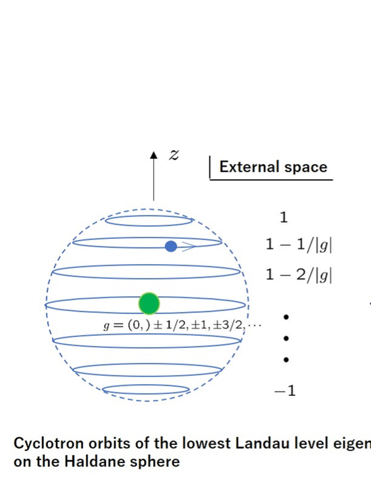
Figure 1: Analogies between the electron cyclotron orbits of the Landau model [70] (left) and the orbits of the quantum spin precession (right).

We leverage this analogy for constructing the generalized gamma matrices of large spin. This idea aligns with the recent developments of non-commutative geometry [53, 54, 55, 56, 57, 57, 58, 59, 60, 61, 62, 63, 64], especially from the quantum matrix geometry of the higher dimensional fuzzy spheres [64, 61, 59, 55, 54]. We present a systematic construction of exactly spherical Bloch hyper-spheres and investigate their exotic properties. We will see that higher dimensional Zeeman-Dirac models necessarily exhibit energy level degeneracies and realize the Wilczek-Zee connections of non-Abelian monopoles. We also investigate implications of Bloch hyper-balls in mixed states and quantum statistics.

This paper is organized as follows. In Sec.2, we review the original Bloch sphere and the spin-coherent states. Section 3 introduces the $SO(5)$ Zeeman-Dirac models and investigate their geometric structures. In Sec.4, we construct $SO(4)$ Zeeman-Dirac models and clarify their properties. We extend the discussions to the general orthogonal groups in Sec.5. In Sec.6, we introduce the density matrices associated with Bloch hyper-balls and discuss their statistical properties such as von Neumann entropy and Bures information metric. Sec.7 is devoted to summary and discussions.

2 Bloch sphere and the $SO(3)$ Zeeman-Dirac model

As a warm-up, we review the Bloch sphere and the spin-coherent states with emphasis on their relation to the $SO(3)$ Zeeman-Dirac model. We will clarify the relationship between the spin-coherent states and the Landau level eigenstates.

2.1 Minimal spin model

We introduce the $SO(3)$ minimal Zeeman-Dirac model:

$$H=\sum_{i=1}^{3}x_{i}\cdot\frac{1}{2}\sigma_{i},$$ (4)

where $x_{i}$ denote the coordinates on $S^{2}$ and play the role of the Bloch vector:

$$x_{1}=\cos\phi\sin\theta,~{}~{}x_{2}=\sin\phi\sin\theta,~{}~{}x_{3}=\cos\theta.$$ (5)

It is easy to solve the eigenvalue problem of this $2\times 2$ matrix Hamiltonian (4):

$$H\Phi^{(\lambda)}=\lambda\cdot\Phi^{(\lambda)},$$ (6)

where the eigenvalues are

$$\lambda=+{1}/{2},-{1}/{2}.$$ (7)

The corresponding eigenstates are known as the spin-coherent states

$$\Phi^{(+\frac{1}{2})}=\frac{1}{\sqrt{2(1+x_{3})}}\begin{pmatrix}1+x_{3}\\ x_{1}+ix_{2}\end{pmatrix}=\begin{pmatrix}\cos(\frac{\theta}{2})\\ \sin(\frac{\theta}{2})e^{i\phi}\end{pmatrix},~{}~{}\Phi^{(-\frac{1}{2})}=\frac{1}{\sqrt{2(1+x_{3})}}\begin{pmatrix}-x_{1}+ix_{2}\\ 1+x_{3}\end{pmatrix}=\begin{pmatrix}-\sin(\frac{\theta}{2})e^{-i\phi}\\ \cos(\frac{\theta}{2})\end{pmatrix},$$ (8)

which are normalized as

$${\Phi^{(+\frac{1}{2})}}^{\dagger}\Phi^{(+\frac{1}{2})}={\Phi^{(-\frac{1}{2})}}^{\dagger}\Phi^{(-\frac{1}{2})}=1,~{}~{}~{}~{}{\Phi^{(+\frac{1}{2})}}^{\dagger}\Phi^{(-\frac{1}{2})}=0.$$ (9)

Notice that the eigenvalues (7) are the diagonal components of $\frac{1}{2}\sigma_{3}$, which is the $U(1)$ sub-algebra of the $SU(2)$. Consequently, the eigenstates (8) carry the quantum numbers of the $U(1)$. The eigenvalues $\lambda=\pm 1/2$ have a nice geometric meaning as the latitudes on the Bloch sphere at which the spin-coherent states are oriented (see the left of Fig.2). We can generate the spin-coherent states by the following well known geometric manipulation. The projection of the Bloch vector $x_{i}$ to the $xy$-plane is given by

$$y_{1}=\cos\phi,~{}~{}y_{2}=\sin\phi.$$ (10)

The spin-coherent state with $\lambda=+1/2$ can be obtained by the rotation of the north-pole oriented spin-coherent state around the $\epsilon_{\mu\nu}y_{\nu}$-axis by $\theta$ (see the right of Fig.2).

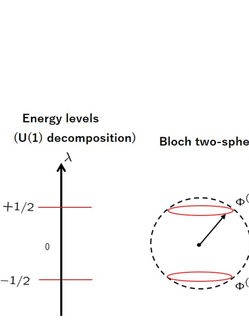
Figure 2: The eigenvalues and the eigenstates of the $SO(3)$ Zeeman-Dirac model (left and middle) and the rotation of the spin (right).

Such a manipulation is demonstrated by the non-linear realization matrix

$$\Phi=e^{-i{\theta}\sum_{\mu,\nu=1}^{2}\epsilon_{\mu\nu}y_{\mu}\frac{1}{2}\sigma_{\nu}},$$ (11)

which is expanded as

$$\Phi =\cos(\frac{\theta}{2})1_{2}-i\sin(\frac{\theta}{2})\sum_{\mu,\nu=1}^{2}\epsilon_{\mu\nu}y_{\mu}\sigma_{\nu}=\begin{pmatrix}\cos\frac{\theta}{2}&-\sin\frac{\theta}{2}e^{-i\phi}\\ \sin\frac{\theta}{2}e^{i\phi}&\cos\frac{\theta}{2}\end{pmatrix}$$

$$=\frac{1}{\sqrt{2(1+x_{3})}}((1+x_{3})1_{2}-i\epsilon_{\mu\nu}x_{\mu}\sigma_{\nu})=\frac{1}{\sqrt{2(1+x_{3})}}\begin{pmatrix}1+x_{3}&-x_{1}+ix_{2}\\ x_{1}+ix_{2}&1+x_{3}\end{pmatrix}.$$ (12)

The spin-coherent states (8) are indeed obtained from $\Phi$ as

$$\Phi^{(+\frac{1}{2})}=\Phi\begin{pmatrix}1\\ 0\end{pmatrix},~{}~{}~{}\Phi^{(-\frac{1}{2})}=\Phi\begin{pmatrix}0\\ 1\end{pmatrix}$$ (13)

or

$$\Phi=\begin{pmatrix}\Phi^{(+\frac{1}{2})}&\Phi^{(-\frac{1}{2})}\end{pmatrix}.$$ (14)

As $\Phi$ has a clear geometric meaning and accommodates the two spin-coherent states simultaneously as its columns, we will utilize the non-linear realization matrix (11) rather than the spin-coherent states themselves. Obviously, $\Phi$ signifies a unitary matrix that diagonalizes the Zeeman-Dirac Hamiltonian:

$$\Phi^{\dagger}H\Phi=\frac{1}{2}\sigma_{3}.$$ (15)

It is important to note that the diagonalization can be justified solely from the group theoretical properties of the $SU(2)$. Solving eigenvalue problems for large-sized matrix Hamiltonians can be laborious. However, the geometric method makes it feasible, as the properties of the $SU(2)$ group are universal regardless of the magnitude of spin. Non-linear realization matrix $\Phi$ (11) is factorized as

$$\Phi=e^{-i\frac{\phi}{2}\sigma_{3}}e^{-i\frac{\theta}{2}\sigma_{2}}e^{i\frac{\phi}{2}\sigma_{3}}.$$ (16)

Similar factorization also holds for non-linear realization matrix of arbitrary spin. This factorization significantly reduces numerical computation time using $\Phi$, especially for large spin matrices. As observed from (15), $\Phi$ enjoys the $U(1)$ degrees of freedom (apart from the overall $U(1)$)

$$\Phi~{}\rightarrow~{}\Phi\cdot e^{i\frac{\chi}{2}\sigma_{3}},$$ (17)

which corresponds to the degrees of freedom for the relative phase of two spin-coherent states. For the original Hamiltonian (4), this $U(1)$ symmetry acts as

$$e^{-i\frac{\chi}{2}\tilde{\sigma}_{3}}~{}H~{}e^{i\frac{\chi}{2}\tilde{\sigma}_{3}}=H,$$ (18)

where

$$\tilde{\sigma}_{3}\equiv\Phi\sigma_{3}\Phi^{\dagger}=\sum_{i=1}^{3}x_{i}\sigma_{i}~{}(=2H).$$ (19)

The $U(1)$ transformation, $e^{i\frac{\chi}{2}\tilde{\sigma}_{3}}=e^{i\chi\sum_{i=1}^{3}x_{i}\frac{1}{2}\sigma_{i}}$, stands for the $SO(2)$ rotation around the Bloch vector by $\chi$, and so the geometric origin of the $U(1)$ symmetry is understood as the $SO(2)$ stabilizer group of the two-sphere, $S^{2}\simeq SO(3)/SO(2)$. It is also intuitively apparent that the rotations around the Bloch vector do not change the $SO(3)$ Hamiltonian (4). An invariant quantity under the $U(1)$ transformation (17) is given by

$${\Phi^{(\pm 1/2)}}^{\dagger}\sigma_{i}\Phi^{(\pm 1/2)}=\pm x_{i},$$ (20)

which is nothing but the Bloch vector (5). The Berry connections of the spin-coherent states are derived as [8]

$$A^{(\pm\frac{1}{2})}=-i{{\Phi}^{(\pm\frac{1}{2})}}^{\dagger}d{\Phi}^{(\pm\frac{1}{2})}=\pm\frac{1}{2}(1-\cos\theta)d\phi=\mp\frac{1}{2(1+x_{3})}\epsilon_{ij3}x_{j}dx_{i},$$ (21)

which are realized as the diagonal components of the pure $SU(2)$ gauge field:

$$-i\Phi^{\dagger}d\Phi=\begin{pmatrix}A^{(+\frac{1}{2})}&*\\ *&A^{(-\frac{1}{2})}\end{pmatrix}.$$ (22)

The $U(1)$ degrees of freedom (15) formally correspond to the $U(1)$ gauge transformations through (22):

$$A^{(\pm\frac{1}{2})}~{}~{}\rightarrow~{}~{}A^{(\pm\frac{1}{2})}\pm\frac{1}{2}d\chi.$$ (23)

The Berry connection (21) is exactly equal to the monopole gauge field with magnetic charge $\lambda=\pm 1/2$. There may arise a natural question about the relationship between the Zeeman-Dirac model and the Landau model. Let us recall the $SO(3)$ Landau model in the $U(1)$ monopole background (see [53] for instance). The degenerate lowest Landau level eigenstates of monopole charge $\pm 1/2$ are given by the monopole harmonics [26]

$$\lambda=+\frac{1}{2}~{}~{}:~{}~{}\phi_{1}^{(+\frac{1}{2})}=\cos(\frac{\theta}{2}),~{}~{}~{}\phi_{2}^{(+\frac{1}{2})}=\sin(\frac{\theta}{2})~{}e^{-i\phi},$$ (25a)

$$\lambda=-\frac{1}{2}~{}~{}:~{}~{}\phi_{1}^{(-\frac{1}{2})}=-\sin(\frac{\theta}{2})~{}e^{i\phi},~{}~{}~{}\phi_{2}^{(-\frac{1}{2})}=\cos(\frac{\theta}{2}).$$ (25b)

Interestingly, these lowest Landau level eigenstates constitute the spin-coherent states (8):

$$\Phi^{(+\frac{1}{2})}=\begin{pmatrix}{\phi_{1}^{(+\frac{1}{2})}}^{*}\\ {\phi_{2}^{(+\frac{1}{2})}}^{*}\\ \end{pmatrix},~{}~{}~{}\Phi^{(-\frac{1}{2})}=\begin{pmatrix}{\phi_{1}^{(-\frac{1}{2})}}^{*}\\ {\phi_{2}^{(-\frac{1}{2})}}^{*}\\ \end{pmatrix}.$$ (26)

2.2 Large spin model

We extend the previous discussions to arbitrary $SU(2)$ spin matrices $(S=0,1/2,1,3/2,\cdots)$, which satisfy $[S_{i},S_{j}]=i\epsilon_{ijk}S_{k}$ and

$$\sum_{i=1}^{3}S_{i}S_{i}=S(S+1)\boldsymbol{1}_{2S+1}.$$ (27)

The matrix components of the spin matrices are given by

$$(S_{x})_{mn}=\frac{1}{2}(\sqrt{(S+m)(S-n)}~{}\delta_{m-1,n}+\sqrt{(S-m)(S+n)}~{}\delta_{m,n-1}),$$

$$(S_{y})_{mn}=i\frac{1}{2}(\sqrt{(S+m)(S-n)}~{}\delta_{m-1,n}-\sqrt{(S-m)(S+n)}~{}\delta_{m,n-1}),$$

$$(S_{z})_{mn}=m\delta_{m,n}.~{}~{}~{}~{}(m,n=S,S-1,S-2,\cdots,-S)$$ (28)

The $S_{z}$ is a diagonal matrix,

$$S_{z}=\begin{pmatrix}S&0&0&0&0\\ 0&S-1&0&0&0\\ 0&0&S-2&0&0\\ 0&0&0&\ddots&0\\ 0&0&0&0&-S\end{pmatrix}.$$ (29)

The $SO(3)$ Hamiltonian (4) is simply generalized as

$$H=\sum_{i=1}^{3}x_{i}S_{i}.$$ (30)

As indicated before, we apply the geometric method to solve the eigenvalue problem of (30):

$$\Phi^{\dagger}H\Phi=S_{3},$$ (31)

where $\Phi$ denotes the non-linear realization matrix

$$\Phi=e^{-i\theta\sum_{\mu,\nu=1}^{2}\epsilon_{\mu,\nu}y_{\mu}S_{\nu}}=e^{-i\phi S_{3}}e^{-i\theta S_{2}}e^{i\phi S_{3}}.$$ (32)

In the notation

$$\Phi\equiv(\Phi^{(S)}~{}\Phi^{(S-1)}~{}\Phi^{(S-2)}~{}\cdots~{}\Phi^{(-S)}),$$ (33)

(31) is restated as

$$H\Phi^{(\lambda)}=\lambda\cdot\Phi^{(\lambda)},$$ (34)

where

$$\lambda=S,~{}S-1,~{}S-2,~{}\cdots,-S.$$ (35)

The $SO(3)$ spin-coherent state $\Phi^{(\lambda)}$ is realized as the $\lambda$th column of the $\Phi$ and denotes the spin coherent state oriented to the latitude $\lambda$ on the Bloch sphere. Note that the spectra of $H$ are nicely illustrated as the latitudes on the Bloch sphere (Fig.3). As $\Phi$ is a unitary matrix, the $\Phi^{(\lambda)}$ apparently satisfy the ortho-normal relations

$${\Phi^{(\lambda)}}^{\dagger}\Phi^{(\lambda^{\prime})}=\delta_{\lambda\lambda^{\prime}}.$$ (36)

Equation (31) is invariant under the $U(1)$ transformation

$$\Phi~{}~{}\rightarrow~{}~{}\Phi\cdot e^{i\chi S_{3}}$$ (37)

or

$$\Phi^{(\lambda)}~{}~{}\rightarrow~{}~{}\Phi^{(\lambda)}e^{i\lambda\chi}.$$ (38)

An $U(1)$-invariant quantity is given by the Bloch vector:

$${\Phi^{(\lambda)}}^{\dagger}S_{i}\Phi^{(\lambda)}=\lambda\cdot x_{i}.$$ (39)

Another important $U(1)$ invariant quantity is the quantum geometric tensor [72]

$$\chi_{\mu\nu}^{(\lambda)}=\partial_{\theta_{\mu}}{\Phi^{(\lambda)}}^{\dagger}\partial_{\theta_{\nu}}{\Phi^{(\lambda)}}-\partial_{\theta_{\mu}}{\Phi^{(\lambda)}}^{\dagger}{\Phi^{(\lambda)}}~{}{\Phi^{(\lambda)}}^{\dagger}\partial_{\theta_{\nu}}{\Phi^{(\lambda)}}.~{}~{}~{}(\theta_{\mu}=\theta,\phi)$$ (40)

The symmetric part of $\chi_{\mu\nu}^{(\lambda)}$ provides the metric of two-sphere:

$$g^{(\lambda)}_{\theta_{\mu}\theta_{\nu}}=\frac{1}{2}(\chi^{(\lambda)}_{\theta_{\mu}\theta_{\nu}}+\chi^{(\lambda)}_{\theta_{\nu}\theta_{\mu}})=\frac{1}{2}(S(S+1)-\lambda^{2})~{}g_{\theta_{\mu}\theta_{\nu}}^{(S_{2})}$$ (41)

with

$$g_{\theta_{\mu}\theta_{\nu}}^{(S^{2})}=\text{diag}(g^{S^{2}}_{\theta\theta},g_{\phi\phi}^{S^{2}})=\text{diag}(1,~{}\sin^{2}\theta).$$ (42)

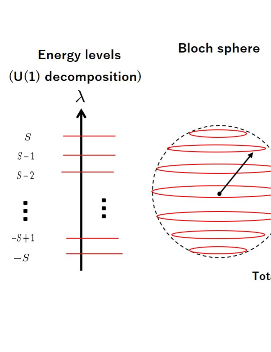
Figure 3: The Bloch sphere with large spin $S$ and the $SO(3)$ spin-coherent state ${\Phi}^{(\lambda)}$ in $\Phi$.

The Berry phase associated with the spin-coherent state $\Phi^{(\lambda)}$ can be derived as

$$-i\Phi^{\dagger}d\Phi=\begin{pmatrix}A^{(S)}&*&*&*\\ *&A^{(S-1)}&*&*\\ *&*&\ddots&*\\ *&*&*&A^{(-S)}\end{pmatrix}$$ (43)

or

$$A^{(\lambda)}=-i{\Phi^{(\lambda)}}^{\dagger}d\Phi^{(\lambda)}=-\lambda\frac{1}{1+x_{3}}\epsilon_{ij3}x_{j}dx_{i}=\lambda(1-\cos\theta)d\phi.$$ (44)

The corresponding field strength $F^{(\lambda)}=dA^{(\lambda)}=\frac{1}{2}F^{(\lambda)}_{\theta_{\mu}\theta_{\nu}}d\theta_{\mu}\wedge d\theta_{\nu}$ is the anti-symmetric part of the quantum geometric tensor:

$$F^{(\lambda)}_{\theta_{\mu}\theta_{\nu}}=-i(\chi^{(\lambda)}_{\theta_{\mu}\theta_{\nu}}-\chi^{(\lambda)}_{\theta_{\nu}\theta_{\mu}})=\lambda\sin(\theta)\epsilon_{\mu\nu},$$ (45)

which is also a $U(1)$ gauge invariant quantity. One may notice that the energy eigenvalue $\lambda$ plays the role of the monopole charge in (44). The corresponding first Chern number is evaluated as

$$\text{ch}_{1}^{(\lambda)}=\frac{1}{2\pi}\int F^{(\lambda)}=2\lambda=\text{sgn}(\lambda)\cdot D_{SO(3)}(|\lambda|-\frac{1}{2})=-\text{ch}_{1}^{(-\lambda)},$$ (46)

where

$$D_{SO(3)}(S)\equiv 2S+1.$$ (47)

Reference [61] discussed the embedding of the Landau level eigenstates in the non-linear realization matrix $\Phi$. Assume that $g$ denotes the monopole charge and $N$ signifies the Landau level index. For the $SU(2)$ spin index, we have the identification

$$S=N+|g|,$$ (48)

and for the $U(1)$ index,

$$S-\lambda=N-g+|g|.$$ (49)

The quantities on the left-hand sides of (48) and (49) come from the $SO(3)$ Zeeman-Dirac model, while those on the right-hand sides come from the $SO(3)$ Landau model. From (48) and (49), we have

$$N=S-|\lambda|,~{}~{}~{}g=\lambda.$$ (50)

Assume that $\phi_{1}^{(g)},\phi_{2}^{(g)},\cdots,\phi_{2S+1}^{(g)}$ stand for the $N=(S-|g|)$th Landau level eigenstates in the $U(1)$ monopole background with charge $g$ (Fig.4). The $SO(3)$ spin-coherent state is represented as

$$\Phi^{(\lambda)}=\begin{pmatrix}{\phi_{1}^{(\lambda)*}}\\ {\phi_{2}^{(\lambda)*}}\\ \vdots\\ {\phi_{2S+1}^{(\lambda)*}}\\ \end{pmatrix},$$ (53)

which represents the precise relationship between the spin-coherent states and the monopole harmonics: The spin-coherent states of large spin $S$ thus consist of the $(2S+1)$-fold degenerate Landau level eigenstates of $N=S-|\lambda|$ in the monopole background with charge $\lambda$ (Fig.4).

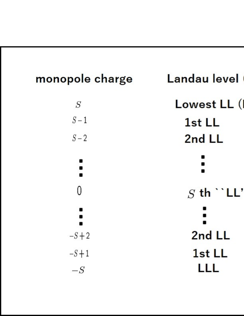
Figure 4: Correspondence between the monopole harmonics and the $SO(3)$ spin-coherent states.

In the above discussions, we started from the Zeeman-Dirac model and later addressed the relationship to the Landau model. However, it is also possible to “reverse” the flow of this argument. Suppose that the $SO(3)$ Landau model was firstly given and the Landau level eigenstates were known. We can generate the large spin matrices $S_{i}$ by the following formula

$$\int_{S^{2}}d\Omega_{2}~{}{\phi^{(\lambda)}_{\alpha}}^{*}~{}x_{i}~{}\phi^{(\lambda)}_{\beta}=\frac{4\pi\lambda}{S(S+1)(2S+1)}(S_{i})_{\alpha\beta}.$$ (54)

In the present $SO(3)$ case, as arbitrary spin matrices were already known, this procedure was unnecessary. However in the case of $SO(5)$ and other higher dimensional groups, this procedure is crucial in constructing large spin gamma matrices.

3 Bloch four-sphere and the $SO(5)$ Zeeman-Dirac model

Here, we extend the results of Sec.2 to the $SO(5)$ Zeeman-Dirac model. The basic idea is based on the analogy between the cyclotron motion on a four-sphere and the $SO(5)$ spin precession in internal space.

3.1 Minimal spin model

The geometric phase of the minimal $SO(5)$ Zeeman-Dirac model [40, 41] has been investigated in Refs.[47, 48, 49]. Here, we reproduce the previous results using the group theoretical method.

We adopt the following $SO(5)$ gamma matrices

$$\gamma_{\mu=1,2,3,4}=\begin{pmatrix}0&\bar{q}_{\mu}\\ q_{\mu}&0\end{pmatrix},~{}~{}\gamma_{5}=\begin{pmatrix}\boldsymbol{1}_{2}&0\\ 0&-\boldsymbol{1}_{2}\end{pmatrix}.~{}~{}~{}~{}~{}~{}(~{}q_{\mu}=\{-i\sigma_{i},\boldsymbol{1}_{2}\},~{}~{}~{}\bar{q}_{\mu}=\{i\sigma_{i},\boldsymbol{1}_{2}\}~{})$$ (55)

These satisfy

$$\{\gamma_{a},\gamma_{b}\}=2\delta_{ab}\boldsymbol{1}_{4}~{}~{}~{}~{}(a,b=1,2,3,4,5)$$ (56)

and yield the $SO(5)$ generators as

$${\sigma}_{ab}=-i\frac{1}{4}[\gamma_{a},\gamma_{b}],$$ (57)

or

$$\sigma_{\mu\nu}=\frac{1}{2}\begin{pmatrix}\eta_{\mu\nu}^{(+)i}\sigma_{i}&0\\ 0&\eta_{\mu\nu}^{(-)i}\sigma_{i}\end{pmatrix},~{}~{}~{}\sigma_{\mu 5}=i\frac{1}{2}\begin{pmatrix}0&\bar{q}_{\mu}\\ -q_{\mu}&0\end{pmatrix}=-\sigma_{5\mu}.$$ (58)

Here, $\eta_{\mu\nu}^{(\pm)i}$ denote the ‘t Hooft tensors,

$$\eta_{\mu\nu}^{(\pm)i}\equiv\epsilon_{\mu\nu i4}\pm\delta_{\mu i}\delta_{\nu 4}\mp\delta_{\nu i}\delta_{\mu 4}.$$ (59)

The minimal $SO(5)$ Zeeman-Dirac Hamiltonian is given by the following $4\times 4$ matrix

$$H=\sum_{a=1}^{5}x_{a}\cdot\frac{1}{2}\gamma_{a},~{}~{}~{}~{}(\sum_{a=1}^{5}x_{a}x_{a}=1)$$ (62)

where $x_{a}$ denote the coordinates of a four-sphere:

$$x_{1}=\cos\phi\sin\theta\sin\chi\sin\xi,~{}~{}x_{2}=\sin\phi\sin\theta\sin\chi\sin\xi,~{}~{}x_{3}=\cos\theta\sin\chi\sin\xi,$$

$$x_{4}=\cos\chi\sin\xi,~{}~{}x_{5}=\cos\xi.$$ (63)

The parameter $\xi$ signifies the azimuthal angle on $S^{4}$. Due to the property (56), the square of $H$ (62) becomes

$$H^{2}=\frac{1}{4}\sum_{a=1}^{5}x_{a}x_{a}\boldsymbol{1}_{4}=\frac{1}{4}\boldsymbol{1}_{4},$$ (64)

which implies that the eigenvalues of $H$ are

$$\lambda=\pm 1/2.$$ (65)

Each eigenvalue is doubly degenerate. In the above diagonalization, we utilized the specific properties of the gamma matrices (56), which $SO(5)$ gamma matrices of large spin do not have. For later convenience, we develop a geometric method for the present case. To orient the $SO(5)$ spin coherent state to the direction $x_{a}$, we introduce the $SO(5)$ non-linear realization matrix [59, 61]:

$$\Psi=e^{i\xi\sum_{\mu=1}^{4}y_{\mu}\sigma_{\mu 5}},$$ (66)

where $y_{\mu}$ denote the coordinates of $S^{3}$-latitude on the four-sphere at the azimuthal angle $\xi$:

$$y_{1}=\cos\phi\sin\theta\sin\chi,~{}~{}y_{2}=\sin\phi\sin\theta\sin\chi,~{}~{}y_{3}=\cos\theta\sin\chi,~{}~{}y_{4}=\cos\chi.$$ (67)

Note the resemblance between (11) and (66). The matrix $\Psi$ is represented by the $S^{4}$ coordinates as

$$\Psi=\cos(\frac{\xi}{2})\boldsymbol{1}_{4}+2i\sin(\frac{\xi}{2})~{}\sum_{\mu=1}^{4}y_{\mu}\sigma_{\mu 5}=\frac{1}{\sqrt{2(1+x_{5})}}\begin{pmatrix}(1+x_{5})\boldsymbol{1}_{2}&-x_{\mu}\bar{q}_{\mu}\\ x_{\mu}{q}_{\mu}&(1+x_{5})\boldsymbol{1}_{2}\end{pmatrix},$$ (68)

which is factorized as

$$\Psi=N(\chi,\theta,\phi)^{\dagger}\cdot e^{i\xi\sigma_{45}}\cdot N(\chi,\theta,\phi)$$ (69)

where

$$N(\chi,\theta,\phi)\equiv e^{i\chi\sigma_{43}}e^{i\theta\sigma_{31}}e^{i\phi\sigma_{12}}.$$ (70)

It is not difficult to check that (68) diagonalizes the $SO(5)$ Hamiltonian,

$$\Psi^{\dagger}H\Psi=\frac{1}{2}\gamma_{5},$$ (71)

or

$$H\Psi=\Psi\frac{1}{2}\gamma_{5}.$$ (72)

In the notation

$$\Psi=\biggl{(}{\Psi}^{(+\frac{1}{2})}~{}\vdots~{}{\Psi}^{(-\frac{1}{2})}\biggr{)}=\biggl{(}{\Psi}^{(+\frac{1}{2})}_{1}~{}{\Psi}^{(+\frac{1}{2})}_{2}~{}\vdots~{}{\Psi}^{(-\frac{1}{2})}_{1}~{}{\Psi}^{(-\frac{1}{2})}_{2}\biggr{)},$$ (73)

the eigenvalue equation (72) is restated as

$$H{\Psi}_{\sigma}^{({\lambda})}=\lambda~{}{\Psi}_{\sigma}^{({\lambda})},$$ (74)

where $\sigma=1,2$ for each of $\lambda=+1/2,-1/2$. The identification (73) indeed reproduces the $SO(5)$ spin-coherent states in the former literatures [47, 48, 49]:

$${\Psi}^{(+\frac{1}{2})}_{1}=\frac{1}{\sqrt{2(1+x_{5})}}\begin{pmatrix}1+x_{5}\\ 0\\ x_{4}-ix_{3}\\ x_{2}-ix_{1}\end{pmatrix},~{}~{}{\Psi}^{(+\frac{1}{2})}_{2}=\frac{1}{\sqrt{2(1+x_{5})}}\begin{pmatrix}0\\ 1+x_{5}\\ -x_{2}-ix_{1}\\ x_{4}+ix_{3}\end{pmatrix},$$ (75a)

$${\Psi}^{(-\frac{1}{2})}_{1}=\frac{1}{\sqrt{2(1+x_{5})}}\begin{pmatrix}-x_{4}-ix_{3}\\ x_{2}-ix_{1}\\ 1+x_{5}\\ 0\end{pmatrix},~{}~{}{\Psi}^{(-\frac{1}{2})}_{2}=\frac{1}{\sqrt{2(1+x_{5})}}\begin{pmatrix}-x_{2}-ix_{1}\\ -x_{4}+ix_{3}\\ 0\\ 1+x_{5}\end{pmatrix}.$$ (75b)

See Fig.5 also.

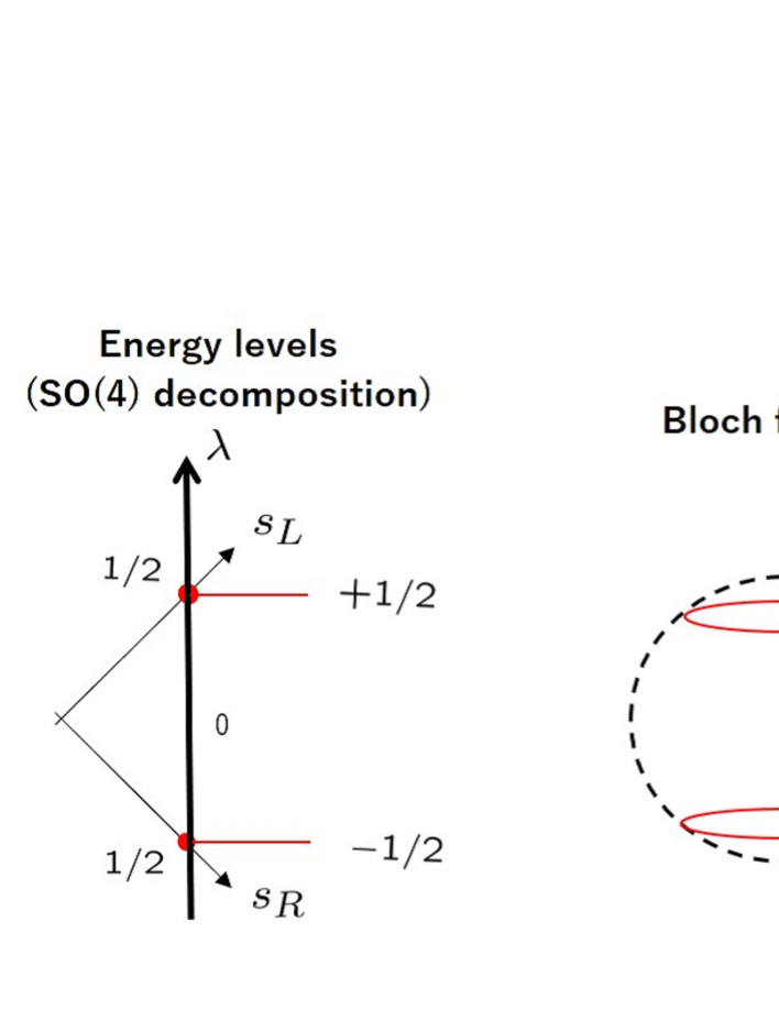
Figure 5: The eigenvalues and the eigenstates of the minimal $SO(5)$ Zeeman-Dirac model.

Since $\gamma_{5}$ is immune to the $SO(4)$ rotations generated by $\sigma_{\mu\nu}$, Eq.(71) implies the existence of the $SO(4)$ symmetry:

$$\Psi~{}~{}\rightarrow~{}~{}\Psi\cdot e^{i\frac{1}{2}\omega_{\mu\nu}\sigma_{\mu\nu}}$$ (76)

or

$$\Psi^{(\pm 1/2)}~{}~{}\rightarrow~{}~{}\Psi^{(\pm 1/2)}\cdot e^{i\frac{1}{4}\eta_{\mu\nu}^{(\pm)i}\omega_{\mu\nu}\sigma_{i}}.$$ (77)

For the original Hamiltonian (62), the $SO(4)$ symmetry is represented as

$$e^{-i\frac{1}{2}\omega_{\mu\nu}\tilde{\sigma}_{\mu\nu}}~{}H~{}e^{i\frac{1}{2}\omega_{\mu\nu}\tilde{\sigma}_{\mu\nu}}=H,$$ (78)

where $\tilde{\sigma}_{\mu\nu}$ denote the $SO(4)$ matrix generators of the form

$$\tilde{\sigma}_{\mu\nu}\equiv\Psi\sigma_{\mu\nu}\Psi^{\dagger}.$$ (79)

Such an $SO(4)$ symmetry is considered to be an “internal” symmetry in the sense that does not change the direction of the Bloch vector $x_{a}$, and the double degeneracy in each energy level is a consequence of such an $SO(4)$ symmetry. The Bloch vector represents an $SO(4)$ invariant quantity:

$${\Psi_{\sigma}^{(\pm\frac{1}{2})}}^{\dagger}\gamma_{a}\Psi^{(\pm\frac{1}{2})}_{\tau}=\pm x_{a}\delta_{\sigma\tau}.$$ (80)

The Wilczek-Zee connections associated with the $SO(5)$ spin-coherent states are derived as

$$A^{(+\frac{1}{2})}=-i{{\Psi}^{(+\frac{1}{2})}}^{\dagger}d{\Psi}^{(+\frac{1}{2})}=-\frac{1}{2(1+x_{5})}\eta_{\mu\nu}^{(+)i}\sigma_{i}x_{\nu}dx_{\mu},$$ (81a)

$$A^{(-\frac{1}{2})}=-i{{\Psi}^{(-\frac{1}{2})}}^{\dagger}d{\Psi}^{(-\frac{1}{2})}=-\frac{1}{2(1+x_{5})}{\eta}_{\mu\nu}^{(-)i}\sigma_{i}x_{\nu}dx_{\mu},$$ (81b)

which are exactly equal to the gauge field configuration of Yang’s $SU(2)$ monopoles [50, 74]. This implies a close relation to the $SO(5)$ Landau model [59, 61]. Assume that $\boldsymbol{\psi}_{\alpha=1,2,3,4}^{(\pm 1/2)}$ denote the lowest Landau level eigenstates in the $SU(2)$ monopole/anti-monopole with the second Chern number $+1/-1$. They are embedded in $\Psi$ (73) as

$$\Psi^{\dagger}=\begin{pmatrix}\boldsymbol{\psi}_{1}^{(+\frac{1}{2})}&\boldsymbol{\psi}_{2}^{(+\frac{1}{2})}&\boldsymbol{\psi}_{3}^{(+\frac{1}{2})}&\boldsymbol{\psi}_{4}^{(+\frac{1}{2})}\\ \boldsymbol{\psi}_{1}^{(-\frac{1}{2})}&\boldsymbol{\psi}_{2}^{(-\frac{1}{2})}&\boldsymbol{\psi}_{3}^{(-\frac{1}{2})}&\boldsymbol{\psi}_{4}^{(-\frac{1}{2})}\end{pmatrix}$$ (83)

or

$$\Psi^{(+\frac{1}{2})}=(\Psi_{1}^{(+\frac{1}{2})}~{}\Psi_{2}^{(+\frac{1}{2})})=\begin{pmatrix}{\boldsymbol{\psi}_{1}^{(+\frac{1}{2})}}^{\dagger}\\ {\boldsymbol{\psi}_{2}^{(+\frac{1}{2})}}^{\dagger}\\ {\boldsymbol{\psi}_{3}^{(+\frac{1}{2})}}^{\dagger}\\ {\boldsymbol{\psi}_{4}^{(+\frac{1}{2})}}^{\dagger}\end{pmatrix},~{}~{}~{}~{}~{}\Psi^{(-\frac{1}{2})}=(\Psi_{1}^{(-\frac{1}{2})}~{}\Psi_{2}^{(-\frac{1}{2})})=\begin{pmatrix}{\boldsymbol{\psi}_{1}^{(-\frac{1}{2})}}^{\dagger}\\ {\boldsymbol{\psi}_{2}^{(-\frac{1}{2})}}^{\dagger}\\ {\boldsymbol{\psi}_{3}^{(-\frac{1}{2})}}^{\dagger}\\ {\boldsymbol{\psi}_{4}^{(-\frac{1}{2})}}^{\dagger}\end{pmatrix}.$$ (84)

3.2 Large spin model

Now we explore $SO(5)$ Zeeman-Dirac models with large spin. To construct large spin $SO(5)$ gamma matrices, we utilize the Landau level eigenstates of the $SO(5)$ Landau model. [64]. We take the matrix elements of the four-sphere coordinates with the (lowest) Landau level eigenstates

$$(\Gamma_{a})_{\alpha\beta}=2(S+2)\int_{S^{4}}d\Omega_{4}~{}\psi_{\alpha}^{\dagger}~{}x_{a}~{}\psi_{\beta},$$ (85)

where $\alpha$ runs from 1 to

$$D_{SO(5)}(S)=\frac{1}{3}(S+1)(2S+1)(2S+3).$$ (86)

Explicit matrix forms of $\Gamma_{a}$ are given by

$$(\Gamma_{\mu})_{(s_{L}^{\prime},m^{\prime}_{L},s_{R}^{\prime},m^{\prime}_{R};~{}s_{L},m_{L},s_{R},m_{R})} =-2~{}\biggl{(}\sqrt{(S-\lambda+1)(S+\lambda+2)}~{}Y_{\mu}^{(+,-)}(s_{L},s_{R})_{(m^{\prime}_{L};m^{\prime}_{R}|m_{L};m_{R})}\delta_{s_{L}^{\prime},s_{L}+\frac{1}{2}}\delta_{s_{R}^{\prime},s_{R}-\frac{1}{2}}$$

$$~{}~{}~{}~{}~{}~{}~{}+\sqrt{(S+\lambda+1)(S-\lambda+2)}~{}Y_{\mu}^{(-,+)}(s_{L},s_{R})_{(m^{\prime}_{L};m^{\prime}_{R}|m_{L};m_{R})}\delta_{s_{L}^{\prime},s_{L}-\frac{1}{2}}\delta_{s_{R}^{\prime},s_{R}+\frac{1}{2}}\biggr{)},$$ (87a)

$$(\Gamma_{5})_{(s_{L}^{\prime},m^{\prime}_{L},s_{R}^{\prime},m^{\prime}_{R};~{}s_{L},m_{L},s_{R},m_{R})} =2\lambda\delta_{s_{L}^{\prime}s_{L}}\delta_{s_{R}^{\prime}s_{R}}\delta_{m^{\prime}_{L}m_{L}}\delta_{m^{\prime}_{R},m_{R}},$$ (87b)

where $s_{L}$, $s_{R}$, $s_{L}^{\prime}$ and $s_{R}^{\prime}$ are non-negative integers or half-integers subject to $s_{L}^{\prime}+s_{R}^{\prime}=s_{L}+s_{R}=S$ and $\lambda\equiv s_{L}-s_{R}$. The quantities, $Y_{\mu}^{(+,-)}(s_{L},s_{R})$ and $Y_{\mu}^{(-,+)}(s_{L},s_{R})$, are defined in [59]. For $S=1/2$, $\Gamma_{a}$ (87) are reduced to the original $SO(5)$ gamma matrices (55). For $S=1$, see Appendix A.

Matrices $\Gamma_{a}$ (87) can be regarded as a natural generalization of the gamma matrices, as they satisfy

$$\sum_{a=1}^{5}\Gamma_{a}\Gamma_{a}=4S(S+2)\boldsymbol{1}_{D_{SO(5)}(S)},$$ (90a)

$$[\Gamma_{a},\Gamma_{b},\Gamma_{c},\Gamma_{d}]=-16(S+1)\epsilon_{abcde}\Gamma_{e},$$ (90b)

where $[~{},~{},~{},~{}]$ represents the Nambu four-bracket that denotes the total antisymmetric combination of the four entities inside the bracket. These relations (90) are exactly equal to the definition of the fuzzy four-sphere [75, 76]. The $SO(5)$ matrix generators $\Sigma_{ab}$ with matrix dimension (86) can be obtained from the commutators of the $\Gamma_{a}$s:

$$\Sigma_{ab}=-i\frac{1}{4}[\Gamma_{a},\Gamma_{b}].$$ (91)

Matrices $\Gamma_{a}$ transform as an $SO(5)$ vector,

$$[\Sigma_{ab},\Gamma_{c}]=i\delta_{ac}\Gamma_{b}-i\delta_{bc}\Gamma_{a},$$ (92)

or

$$\Gamma_{a}~{}~{}\rightarrow~{}~{}R_{ab}\Gamma_{b},$$ (93)

with $R_{ab}\equiv e^{i\frac{1}{2}\omega_{ab}\Sigma_{ab}^{\text{(vec)}}}~{}~{}((\Sigma_{ab}^{\text{(vec)}})_{cd}\equiv-i\delta_{ac}\delta_{bd}+i\delta_{ad}\delta_{bc})$ being $SO(5)$ group elements,

$$R_{ac}R_{bc}=\delta_{ab},~{}~{}~{}~{}~{}\epsilon_{abcde}R_{aa^{\prime}}R_{bb^{\prime}}R_{cc^{\prime}}R_{dd^{\prime}}=\epsilon_{a^{\prime}b^{\prime}c^{\prime}d^{\prime}e^{\prime}}R_{ee^{\prime}}.$$ (94)

It is obvious that (90) are $SO(5)$ covariant equations, which demonstrate the $SO(5)$ spherical symmetry of the present system. In the large $S$ limit, Eq.(90a) becomes $\sum_{a=1}^{5}\frac{1}{2}\Gamma_{a}\cdot\frac{1}{2}\Gamma_{a}\sim S^{2}\boldsymbol{1}_{D_{SO(5)}(S)}$, implying that $\frac{1}{2}\Gamma_{a}$ represent quantum spin matrices of the magnitude $S$. The diagonal matrix $\frac{1}{2}\Gamma_{5}$ (87b) is represented as

$$\frac{1}{2}\Gamma_{5}=\begin{pmatrix}S\boldsymbol{1}_{2S+1}&0&0&0&0\\ 0&(S-1)\boldsymbol{1}_{4S}&0&0&0\\ 0&0&(S-2)\boldsymbol{1}_{3(2S-1)}&0&0\\ 0&0&0&\ddots&0\\ 0&0&0&0&-S\boldsymbol{1}_{2S+1}\\ \end{pmatrix}=\bigoplus_{\lambda=-S}^{S}\lambda~{}\boldsymbol{1}_{D_{SO(4)}(s_{L},s_{R})},$$ (95)

where

$$D_{SO(4)}(s_{L},s_{R})=(2s_{L}+1)(2s_{R}+1)=(S+\lambda+1)(S-\lambda+1)$$ (96)

with bi-spin index of $SU(2)_{L}\otimes SU(2)_{R}\simeq SO(4)$:

$$s_{L}\equiv\frac{S}{2}+\frac{\lambda}{2},~{}~{}~{}~{}s_{R}\equiv\frac{S}{2}-\frac{\lambda}{2}.$$ (97)

Notice that $\frac{1}{2}\Gamma_{5}$ (95) is exactly equal to $S_{z}$ (29) up to the degeneracies.

We now introduce an $SO(5)$ large spin Zeeman-Dirac Hamiltonian as

$$H=\sum_{a=1}^{5}x_{a}\cdot\frac{1}{2}\Gamma_{a}.~{}~{}~{}~{}(\sum_{a=1}^{5}x_{a}x_{a}=1)$$ (98)

Since the $\Gamma_{a}$ behave as an $SO(5)$ vector, we can safely apply the group theoretical method to diagonalize this Hamiltonian. Replacing $\sigma_{ab}$ with $\Sigma_{ab}$ (91), we readily obtain

$$\Psi=e^{i\xi\sum_{\mu=1}^{4}y_{\mu}\Sigma_{\mu 5}}={N}(\chi,\theta,\phi)^{\dagger}\cdot e^{-i\xi\Sigma_{45}}\cdot N(\chi,\theta,\phi),~{}~{}~{}~{}~{}(N(\chi,\theta,\phi)\equiv e^{i\chi\Sigma_{43}}e^{i\theta\Sigma_{31}}e^{i\phi\Sigma_{12}})$$ (99)

which diagonalizes the Hamiltonian,

$$\Psi^{\dagger}H\Psi=\frac{1}{2}\Gamma_{5}.$$ (100)

The eigenvalues of the $SO(5)$ Hamiltonian ranges from $-S$ to $S$ with each interval between the adjacent eigenvalues being $1$. As the eigenvalues approach zero, the degeneracy $D_{SO(4)}(s_{L},s_{R})$ increases (Fig.6).

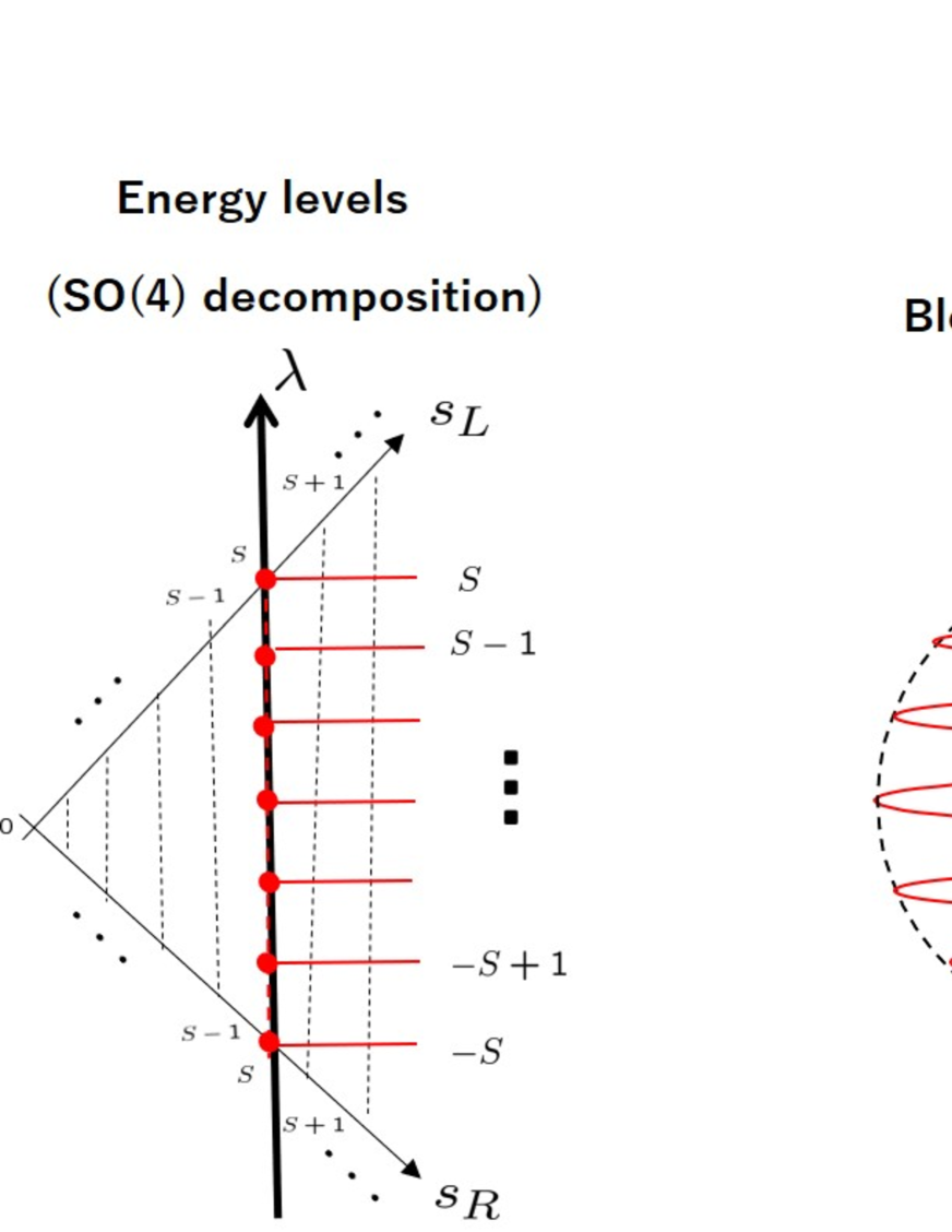
Figure 6: The $SO(5)$ Zeeman-Dirac model with large spin $S$.

The explicit degenerate eigenstates can be identified from the non-linear realization matrix (Fig.7):

$$\Psi =\biggl{(}\Psi^{(S)}~{}\vdots~{}\Psi^{(S-1)})~{}\vdots~{}\Psi^{(S-2)})~{}\vdots~{}\cdots~{}\vdots~{}\Psi^{(-S)}\biggr{)}$$

$$=\biggl{(}{\Psi}^{(S)}_{1}\cdots{\Psi}^{(S)}_{2S+1}~{}\vdots~{}{\Psi}^{(S-1)}_{1}\cdots{\Psi}^{(S-1)}_{4S}~{}\vdots~{}{\Psi}^{(S-2)}_{1}\cdots{\Psi}^{(S-2)}_{3(2S-1)}~{}\vdots~{}\cdots\cdots\cdots\!~{}\vdots~{}{\Psi}^{(-S)}_{1}\cdots{\Psi}^{(-S)}_{2S+1}\biggr{)}.$$ (101)

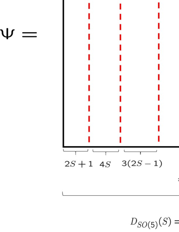
Figure 7: The $SO(5)$ spin-coherent state matrix ${\Psi}^{(\lambda)}$ in $\Psi$.

The columns ${\Psi}_{\sigma}^{(\lambda)}$ $(\lambda=S,S-1,\cdots,-S,~{}\sigma=1,2,\cdots,D_{SO(4)}(s_{L},s_{R}))$ denote the $SO(5)$ spin-coherent states that satisfy

$$\sum_{a=1}^{5}(x_{a}\cdot\frac{1}{2}\Gamma_{a})\Psi^{(\lambda)}_{\sigma}=\lambda\Psi^{(\lambda)}_{\sigma}.~{}~{}~{}~{}(\sigma=1,2,\cdots,D_{SO(4)}(s_{L},s_{R}))$$ (102)

Their ortho-normal relations are given by

$${\Psi^{(\lambda)}_{\sigma}}^{\dagger}\Psi^{(\lambda^{\prime})}_{\tau}=\delta_{\sigma\tau}\delta_{\lambda\lambda^{\prime}}.$$ (103)

As $\Gamma_{5}$ is immune to the $SO(4)$ transformations, $[\Gamma_{5},\Sigma_{\mu\nu}]=0$, there exist $SO(4)$ degrees of freedom in (100):

$$\Psi~{}~{}\rightarrow~{}~{}\Psi\cdot e^{i\frac{1}{2}\omega_{\mu\nu}\Sigma_{\mu\nu}}.$$ (104)

The Bloch vector is an $SO(4)$ invariant quantity:

$${\Psi^{(\lambda)}}^{\dagger}\Gamma_{a}\Psi^{(\lambda)}=2\lambda\cdot x_{a}\boldsymbol{1}_{D_{SO(4)}(s_{L},s_{R})}.$$ (105)

Unlike the previous $SO(3)$ case, the quantum geometric tensor a matrix-valued $SO(4)$ covariant quantity (not $SO(4)$ invariant):

$$\chi_{\theta_{\mu}\theta_{\nu}}^{(\lambda)}=\partial_{\theta_{\mu}}{\Psi^{(\lambda)}}^{\dagger}\partial_{\theta_{\nu}}{\Psi^{(\lambda)}}-\partial_{\theta_{\mu}}{\Psi^{(\lambda)}}^{\dagger}{\Psi^{(\lambda)}}~{}{\Psi^{(\lambda)}}^{\dagger}\partial_{\theta_{\nu}}{\Psi^{(\lambda)}}.~{}~{}~{}(\theta_{\mu}=\xi,\chi,\theta,\phi)$$ (106)

See Appendix B for more details about the matrix-valued quantum geometric tensor. The trace of its symmetric part gives rise to the metric of a four-sphere:

$$g^{(\lambda)}_{\theta_{\mu}\theta_{\nu}}=\frac{1}{2}\text{tr}(\chi^{(\lambda)}_{\theta_{\mu}\theta_{\nu}}+\chi^{(\lambda)}_{\theta_{\nu}\theta_{\mu}})~{}\propto~{}g_{\theta_{\mu}\theta_{\nu}}^{(S^{4})}=\text{diag}(1,~{}\sin^{2}\xi,~{}\sin^{2}\xi\sin^{2}\chi,~{}\sin^{2}\xi\sin^{2}\chi\sin^{2}\theta)..$$ (107)

The dependence of $S$ and $|\lambda|$ is accounted for by the proportional coefficient.

The Wilczek-Zee connections associated with the $SO(5)$ coherent states are derived as

$$-i\Psi^{\dagger}d\Psi=\begin{pmatrix}A^{(S)}&*&*&*&*\\ *&A^{(S-1)}&*&*&*\\ *&*&\ddots&*&*\\ *&*&*&A^{(-S+1)}&*\\ *&*&*&*&A^{(-S)}\end{pmatrix},$$ (108)

where

$$A^{(\lambda)}=-i{{\Psi}^{(\lambda)}}^{\dagger}d{\Psi}^{(\lambda)}=-\frac{1}{1+x_{5}}\Sigma_{\mu\nu}^{(s_{L},s_{R})}x_{\nu}dx_{\mu}=\frac{1}{2}\omega_{\mu\nu\theta_{\rho}}\Sigma_{\mu\nu}^{(s_{L},s_{R})}d\theta_{\rho}.$$ (109)

Here, $\omega_{\mu\nu\theta_{\rho}}$ denote the spin-connection of $S^{4}$ [59] and $\Sigma_{\mu\nu}^{(s_{L},s_{R})}$ signify the $SO(4)$ matrix generators

$$\Sigma_{\mu\nu}^{(s_{L},s_{R})}\equiv\eta^{(+)i}_{\mu\nu}S_{i}^{(s_{L})}\otimes\boldsymbol{1}_{2s_{R}+1}+\boldsymbol{1}_{2s_{L}+1}\otimes\eta^{(-)i}_{\mu\nu}S_{i}^{(s_{R})},$$ (110)

with $\eta_{\mu\nu}^{(\pm)i}$ being the ’t Hooft tensors (59). The Wilczek-Zee connections $A^{(\lambda)}$ in (109) coincide with the gauge fields of the $SO(4)$ monopoles [61]. The corresponding curvature, $F_{\theta_{\mu}\theta_{\nu}}=\partial_{\theta_{\mu}}A_{\theta_{\nu}}-\partial_{\theta_{\nu}}A_{\theta_{\mu}}+i[A_{\theta_{\mu}},A_{\theta_{\nu}}]$, is equal to the antisymmetric part of (106):

$$F_{\theta_{\mu}\theta_{\nu}}^{(\lambda)}=-i(\chi^{(\lambda)}_{\theta_{\mu}\theta_{\nu}}-\chi^{(\lambda)}_{\theta_{\nu}\theta_{\mu}})=\frac{1}{2}e^{\mu^{\prime}}_{~{}\theta_{\mu}}\wedge e^{\nu^{\prime}}_{~{}\theta_{\nu}}\Sigma_{\mu^{\prime}\nu^{\prime}}^{(s_{L},s_{R})},$$ (112)

where $e^{\mu^{\prime}}_{~{}\theta_{\mu}}$ denote the vierbein of $S^{4}$ [59]. The $SO(4)$ monopole is essentially the composite of the $SU(2)$ monopole and the $SU(2)$ anti-monopole and characterized by the second Chern number and a generalized Euler number [61]:

$$\text{ch}_{2}^{(\lambda)}\equiv\frac{1}{8\pi^{2}}\int_{S^{4}}\text{tr}(F\wedge F)=\frac{1}{8\pi^{2}}\int_{S^{4}}\text{tr}(\mathcal{F}\wedge\mathcal{F})=\frac{2}{3}(S+1)~{}\lambda~{}(S+1+\lambda)(S+1-\lambda),$$ (113a)

$$\tilde{c}_{2}^{(\lambda)}\equiv\frac{1}{8\pi^{2}}\int_{S^{4}}\text{tr}(F\wedge\mathcal{F})=\frac{1}{8\pi^{2}}\int_{S^{4}}\text{tr}(\mathcal{F}\wedge F)=\frac{1}{3}(S(S+2)+\lambda^{2})~{}(S+1+\lambda)(S+1-\lambda),$$ (113b)

where $\mathcal{F}$ stands for the field strength with the replacement of the $SO(4)$ matrix generators $\Sigma^{(s_{L},s_{R})}_{\mu\nu}$ in $F$ (112) by $\frac{1}{2}\epsilon_{\mu\nu\rho\sigma}\Sigma_{\rho,\sigma}^{(s_{L},s_{R})}$. The topological numbers (113) have the reflection symmetry:

$$\text{ch}_{2}^{(\lambda)}=-\text{ch}_{2}^{(-\lambda)},~{}~{}~{}~{}\tilde{c}_{2}^{(\lambda)}=+\tilde{c}_{2}^{(-\lambda)}.$$ (114)

The Atiyah-Singer index theorem tells that [61]

$$\text{ch}_{2}^{(\lambda)}=\text{sgn}(\lambda)\cdot D_{SO(5)}(S-\frac{1}{2},|\lambda|-\frac{1}{2}),$$ (115)

where $\text{sgn}(0)\equiv 0$ and

$$D_{SO(5)}(S-\frac{1}{2},|\lambda|-\frac{1}{2})\equiv\frac{2}{3}(S+1)|\lambda|(S+|\lambda|+1)(S-|\lambda|+1).$$ (116)

The $SO(5)$ spin-coherent state matrices in (101) are represented as

$$\Psi^{(\lambda)}=\begin{pmatrix}{\Psi}^{(\lambda)}_{1}&{\Psi}^{(\lambda)}_{2}&\cdots&{\Psi}^{(\lambda)}_{D_{SO(4)}(s_{L},s_{R})}\end{pmatrix}=\begin{pmatrix}{\boldsymbol{\psi}_{1}^{(\lambda)}}^{\dagger}\\ {\boldsymbol{\psi}_{2}^{(\lambda)}}^{\dagger}\\ {\boldsymbol{\psi}_{3}^{(\lambda)}}^{\dagger}\\ \vdots\\ {\boldsymbol{\psi}_{D_{SO(5)}(S)}^{(\lambda)}}^{\dagger}\\ \end{pmatrix},$$ (117)

where $\boldsymbol{\psi}_{\alpha}^{(\lambda)}$ are the $SO(5)$ Landau level eigenstates of the $SO(4)$ monopole background with the bi-spin index $(s_{L},s_{R})=(\frac{S}{2}+\frac{\lambda}{2},\frac{S}{2}-\frac{\lambda}{2})$ (97). To encapsulate, the correspondence between the spin-coherent states and the Landau level eigenstates is the following:

$$D_{SO(5)}(S)~{}~{}~{}~{}~{}~{}~{}:~{}~{}\text{Dimension of the spin-coherent states}~{}~{}~{}=~{}~{}\text{Degeneracy of the Landau level eigenstates}$$

$$D_{SO(4)}(s_{L},s_{R})~{}:~{}~{}\text{Degeneracy of the spin-coherent states}~{}~{}=~{}~{}\text{Dimension of the Landau level eigenstates}$$

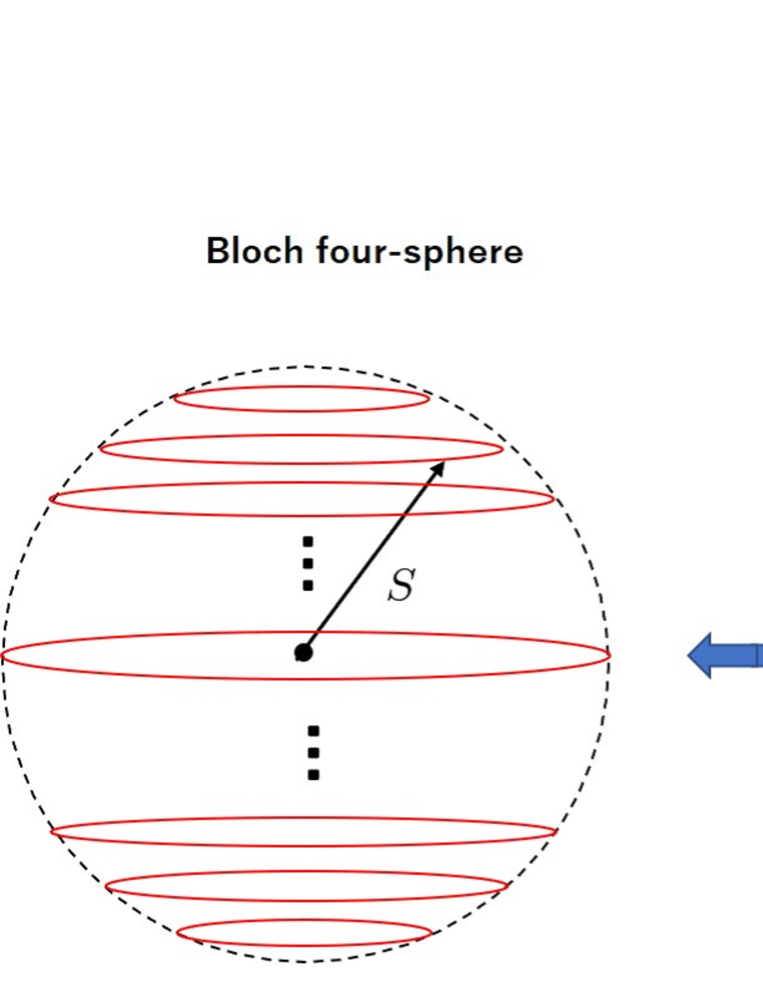
Figure 8: The Bloch four-sphere and the $SO(5)$ Landau level eigenstates.

4 Bloch three-sphere and $SO(4)$ Zeeman-Dirac model

This section discusses the $SO(4)$ Zeeman-Dirac models. Properties of the large spin $SO(4)$ Zeeman-Dirac models are quite distinct from those of the $SO(3)$ and $SO(5)$ models.

4.1 Minimal spin model

With the $SO(4)$ gamma matrices $\gamma_{\mu}$ (55), we construct the minimal $SO(4)$ Zeeman-Dirac model,

$$H=\sum_{\mu=1}^{4}x_{\mu}\cdot\frac{1}{2}\gamma_{\mu}=\frac{1}{2}\begin{pmatrix}0&\sum_{\mu=1}^{4}x_{\mu}\bar{q}_{\mu}\\ \sum_{\mu=1}^{4}x_{\mu}{q}_{\mu}&0\end{pmatrix}.~{}~{}~{}~{}(\sum_{\mu=1}^{4}x_{\mu}x_{\mu}=1)$$ (120)

As the $SO(5)$ minimal Hamiltonian (62) is reduced to (120) on the $S^{3}$-equator ($\xi=\frac{\pi}{2}$) of the four-sphere, they shares similar properties, such as $H^{2}=\frac{1}{4}\boldsymbol{1}_{4}$. With the $S^{3}$-coordinates

$$x_{1}=\sin\theta\cos\phi\sin\chi,~{}~{}x_{2}=\sin\theta\sin\phi\sin\chi,~{}~{}~{}x_{3}=\cos\theta\sin\chi,~{}~{}~{}x_{4}=\cos\chi,$$ (121)

we introduce a unitary matrix in a similar manner to (66)

$$\Psi(\chi,\theta,\phi)=e^{i\chi\sum_{i=1}^{3}y_{i}\sigma_{i4}}=\begin{pmatrix}U(\chi,\theta,\phi)&0\\ 0&U(\chi,\theta,\phi)^{\dagger}\end{pmatrix},~{}~{}~{}~{}(y_{i=1,2,3}\equiv\frac{1}{\sin\chi}x_{i})$$ (123)

where

$$U(\chi,\theta,\phi)\equiv e^{i\frac{\chi}{2}y_{i}\sigma_{i}}=\frac{1}{\sqrt{2(1+x_{4})}}((1+x_{4})\boldsymbol{1}_{2}+ix_{i}\sigma_{i}).$$ (124)

Unitary matrix $\Psi$ transforms the $SO(4)$ minimal Hamiltonian into the form

$$\Psi^{\dagger}H\Psi=\frac{1}{2}\gamma_{4}.$$ (125)

Applying another unitary transformation

$$V\equiv e^{i\frac{\pi}{2}\sigma_{45}}=\frac{1}{\sqrt{2}}\begin{pmatrix}\boldsymbol{1}_{2}&-\boldsymbol{1}_{2}\\ \boldsymbol{1}_{2}&\boldsymbol{1}_{2}\end{pmatrix},~{}~{}~{}~{}~{}(V^{\dagger}\gamma_{4}V=\gamma_{5})$$ (126)

we can diagonalize the $SO(4)$ Hamiltonian (120) as

$$\tilde{\Psi}^{\dagger}H\tilde{\Psi}=\frac{1}{2}\gamma_{5},$$ (127)

where

$$\tilde{\Psi}\equiv\Psi~{}V=\frac{1}{\sqrt{2}}\begin{pmatrix}U&-U\\ U^{\dagger}&U^{\dagger}\end{pmatrix}.$$ (128)

Therefore, the $SO(4)$ spin-coherent states that satisfy

$$H\tilde{\Psi}_{\sigma}^{(\pm\frac{1}{2})}=\pm\frac{1}{2}\tilde{\Psi}_{\sigma}^{(\pm\frac{1}{2})}~{}~{}~{}~{}(\sigma=1,2)$$ (129)

are obtained as

$$\tilde{\Psi}=(~{}\tilde{\Psi}_{1}^{(+\frac{1}{2})}~{}\tilde{\Psi}_{2}^{(+\frac{1}{2})}~{}\vdots~{}\tilde{\Psi}_{1}^{(-\frac{1}{2})}~{}\tilde{\Psi}_{2}^{(-\frac{1}{2})}~{})$$ (130)

where

$$\tilde{\Psi}_{1}^{(+\frac{1}{2})}=\frac{1}{2\sqrt{1+x_{4}}}\begin{pmatrix}1+x_{4}+ix_{3}\\ -x_{2}+ix_{1}\\ 1+x_{4}-ix_{3}\\ x_{2}-ix_{1}\end{pmatrix},~{}~{}\tilde{\Psi}_{2}^{(+\frac{1}{2})}=\frac{1}{2\sqrt{1+x_{4}}}\begin{pmatrix}x_{2}+ix_{1}\\ 1+x_{4}-ix_{3}\\ -x_{2}-ix_{1}\\ 1+x_{4}+ix_{3}\end{pmatrix},$$

$$\tilde{\Psi}_{1}^{(-\frac{1}{2})}=\frac{1}{2\sqrt{1+x_{4}}}\begin{pmatrix}-1-x_{4}-ix_{3}\\ x_{2}-ix_{1}\\ 1+x_{4}-ix_{3}\\ x_{2}-ix_{1}\end{pmatrix},~{}~{}\tilde{\Psi}_{2}^{(-\frac{1}{2})}=\frac{1}{2\sqrt{1+x_{4}}}\begin{pmatrix}-x_{2}-ix_{1}\\ -1-x_{4}+ix_{3}\\ -x_{2}-ix_{1}\\ 1+x_{4}+ix_{3}\end{pmatrix}.$$ (131)

See Fig.9. The eigenvalues and the degeneracies of the $SO(4)$ minimal model are equal to those of the $SO(5)$ minimal model. Equation (125) is invariant under the $SO(3)$ transformation

$$\Psi~{}~{}\rightarrow~{}~{}\Psi\cdot e^{i\frac{1}{2}\omega_{ij}\sigma_{ij}},$$ (132)

where $\sigma_{ij}=\frac{1}{2}\epsilon_{ijk}\begin{pmatrix}\sigma_{k}&0\\ 0&\sigma_{k}\end{pmatrix}$ are the $SO(3)$ matrix generators that commutate with $\gamma_{4}$. This symmetry brings the $SO(3)$ degeneracy to each energy level. The $SO(4)$ Bloch vector can be obtained as an $SO(3)$ gauge invariant quantity

$$({{\tilde{\Psi}}}^{(\pm\frac{1}{2})}_{\sigma})^{\dagger}\gamma_{\mu}{\tilde{\Psi}}_{\tau}^{(\pm\frac{1}{2})}=\pm x_{\mu}\delta_{\sigma\tau}.$$ (133)

In the present case, the doubly degenerate $SO(4)$ spin-coherent states in the upper and lower energy levels provide the identical Wilczek-Zee connections

$${A}\equiv-i\tilde{\Psi}_{1}^{\dagger}d\tilde{\Psi}_{1}=-i\tilde{\Psi}_{2}^{\dagger}d\tilde{\Psi}_{2}=-i\frac{1}{2}(g^{\dagger}dg+gdg^{\dagger})=-\frac{1}{2(1+x_{4})}\epsilon_{ijk}x_{j}dx_{i}\sigma_{k},$$ (134)

which exactly coincides with the $SU(2)$ spin-connection of $S^{3}$ [77, 78].

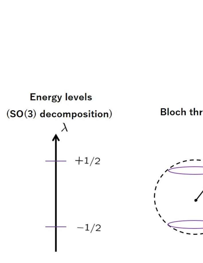
Figure 9: $SO(4)$ minimal Zeeman-Dirac model.

4.2 Large spin model

Construction of the $SO(4)$ Zeeman-Dirac model with large spin is rather tricky. One might consider to adopt ${\Gamma}_{\mu=1,2,3,4}$ (87) as the $SO(4)$ large spin gamma matrices, however $\Gamma_{\mu}$ are not good enough for the purpose. This is because the sum of the squares of $\Gamma_{\mu}$ is not proportional to unit matrix:

$$\sum_{\mu=1}^{4}\Gamma_{\mu}\Gamma_{\mu}~{}\not\propto~{}\boldsymbol{1}.$$ (135)

Generalized gamma matrices with the desired property, $\sum_{\mu=1}^{4}\mathit{\Gamma}_{\mu}\mathit{\Gamma}_{\mu}~{}\propto~{}\boldsymbol{1}$, can be explicitly constructed from the $SO(4)$ Landau model [64, 55, 77] in the subspace [79, 80, 81, 82] (Fig.10):

$$(s_{L},s_{R})=(\frac{S}{2}+\frac{1}{4},\frac{S}{2}-\frac{1}{4})\oplus(\frac{S}{2}-\frac{1}{4},\frac{S}{2}+\frac{1}{4}).~{}~{}~{}(2S~{}:~{}\text{odd})$$ (136)

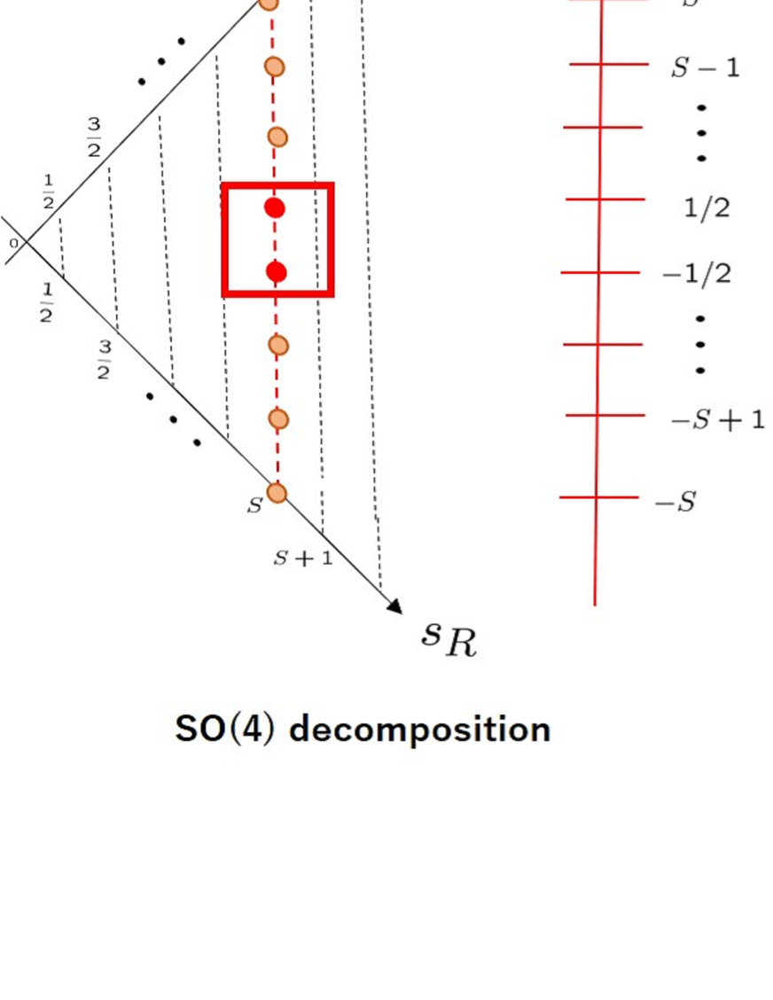
Figure 10: The $SO(4)$ subspace of $(s_{L},s_{R})=(\frac{2S+1}{4},\frac{2S-1}{4})\oplus(\frac{2S-1}{4},\frac{2S+1}{4})$, with dimension, $2\cdot\frac{2S+3}{2}\cdot\frac{2S+1}{2}=\frac{1}{2}(2S+3)(2S+1)$.

The subspace (136) geometrically corresponds to the two latitudes adjacent to the equator of the Bloch four-sphere. The restriction to a sub-space obviously reduces the $SO(5)$ covariance to the $SO(4)$ covariance. It should be noted that $S$ has to be a half-integer value in the $SO(4)$ models, so that $s_{L/R}$ (136) takes integer or half-integer values. The matrix elements of $\mathit{\Gamma}_{\mu}$ in the subspace (136) are given by

$$\mathit{\Gamma}_{\mu}=-(2S+3)\begin{pmatrix}0&Y_{\mu}^{(+,-)}(\frac{2S-1}{4},\frac{2S+1}{4})\\ Y_{\mu}^{(-,+)}(\frac{2S+1}{4},\frac{2S-1}{4})&0\end{pmatrix},~{}~{}~{}(2S~{}:~{}\text{odd})$$ (137)

where $Y_{\mu}^{(+,-)}(\frac{2S-1}{4},\frac{2S+1}{4})$ are square matrices of dimension $\frac{1}{4}(2S+1)(2S+3)\times\frac{1}{4}(2S+1)(2S+3)$ and $Y_{\mu}^{(-,+)}(\frac{2S+1}{4},\frac{2S-1}{4})$ are their Hermitian conjugates. For $S=1/2$, (137) is equal to $\gamma_{\mu}$. For $S=3/2$, see Appendix A.2.

With (138), we can explicitly demonstrate that $\mathit{\Gamma}_{\mu}$ (137) satisfy [64, 55]

$$\sum_{\mu=1}^{4}\mathit{\Gamma}_{\mu}\mathit{\Gamma}_{\mu}=\frac{1}{2}(2S+1)(2S+3)\boldsymbol{1}_{\frac{1}{2}(2S+1)(2S+3)},,$$ (141a)

$$[\![\mathit{\Gamma}_{\mu},\mathit{\Gamma}_{\nu},\mathit{\Gamma}_{\rho}]\!]=16(S+1)\epsilon_{\mu\nu\rho\sigma}\mathit{\Gamma}_{\sigma},$$ (141b)

where $[\![~{}~{},~{}~{},~{}~{}]\!]$ signifies the Nambu “three-bracket” defined by

$$[\![\mathit{\Gamma}_{\mu},\mathit{\Gamma}_{\nu},\mathit{\Gamma}_{\rho}]\!]\equiv[\mathit{\Gamma}_{\mu},\mathit{\Gamma}_{\nu},\mathit{\Gamma}_{\rho},G_{5}]=4[\mathit{\Gamma}_{\mu},\mathit{\Gamma}_{\nu},\mathit{\Gamma}_{\rho}]G_{5}$$ (142)

with

$$G_{5}\equiv\begin{pmatrix}\boldsymbol{1}_{\frac{1}{4}(2S+3)(2S+1)}&0\\ 0&-\boldsymbol{1}_{\frac{1}{4}(2S+3)(2S+1)}\end{pmatrix}.$$ (143)

Equations (141) designate the definition of fuzzy three-sphere [80, 81]. The corresponding $SO(4)$ matrix generators are given by

$$\mathit{\Sigma}_{\mu\nu}\equiv\bigoplus_{\lambda=-\frac{1}{2}}^{\frac{1}{2}}\Sigma_{\mu\nu}^{(\frac{S}{2}+\frac{\lambda}{2},\frac{S}{2}-\frac{\lambda}{2})}=\begin{pmatrix}\Sigma_{\mu\nu}^{(\frac{2S+1}{4},\frac{2S-1}{4})}&0\\ 0&\Sigma_{\mu\nu}^{(\frac{2S-1}{4},\frac{2S+1}{4})}\end{pmatrix}.$$ (144)

Notice that, while the commutators between $\mathit{\Gamma}_{\mu}$ do not yield $SO(4)$ matrix generators (144) (except for $S=1/2$)

$$[\mathit{\Gamma}_{\mu},\mathit{\Gamma}_{\nu}]~{}\neq~{}4i\mathit{\Sigma}_{\mu\nu},$$ (145)

$\mathit{\Gamma}_{\mu}$ behave as an $SO(4)$ vector under the transformation generated by $\mathit{\Sigma}_{\mu\nu}$:

$$[\mathit{\Sigma}_{\mu\nu},\mathit{\Gamma}_{\rho}]=i\delta_{\mu\rho}\mathit{\Gamma}_{\nu}-i\delta_{\nu\rho}\mathit{\Gamma}_{\mu}.$$ (146)

Matrix $G_{5}$ (143) obviously satisfies $[\mathit{\Sigma}_{\mu\nu},G_{5}]=0$ and is immune to the $SO(4)$ transformations generated by $\mathit{\Sigma}_{\mu\nu}$. These properties imply that (141) are $SO(4)$ covariant equations. Note that any of $\mathit{\Gamma}_{\mu}$ is diagonalized as

$$\mathit{\Gamma}_{\mu}~{}~{}~{}\rightarrow~{}~{}\mathit{\Gamma}_{\text{diag}} \equiv\begin{pmatrix}S\boldsymbol{1}_{2S+1}&0&0&0&0\\ 0&(S-1)\boldsymbol{1}_{2S-1}&0&0&0\\ 0&0&(S-2)\boldsymbol{1}_{2S-3}&0&0\\ 0&0&0&\ddots&0\\ 0&0&0&0&-S\boldsymbol{1}_{2S+1}\end{pmatrix}+\frac{1}{2}G_{5}$$

$$=\bigoplus_{\lambda=-S}^{S}(\lambda+\frac{1}{2}\text{sgn}(\lambda))~{}\boldsymbol{1}_{2|\lambda|+1}.$$ (147)

One may find a resemblance between $\mathit{\Gamma}_{\text{diag}}$ (147) and $\frac{1}{2}\Gamma_{5}$ (95). We now introduce a large spin $SO(4)$ Zeeman-Dirac Hamiltonian as

$$H=\sum_{\mu=1}^{4}x_{\mu}\cdot\frac{1}{2}\mathit{\Gamma}_{\mu}.$$ (148)

Due to the $SO(4)$ covariance, the Hamiltonian (148) can be transformed as

$$\mathit{\Psi}^{\dagger}\cdot H\cdot\mathit{\Psi}=\frac{1}{2}\mathit{\Gamma}_{4},$$ (149)

where

$$\mathit{\Psi}=e^{i\chi\sum_{i=1}^{3}y_{i}\mathit{\Sigma}_{i4}}=\begin{pmatrix}e^{i\chi\sum_{i=1}^{3}y_{i}\Sigma_{i4}^{(\frac{2S+1}{4},\frac{2S-1}{4})}}&0\\ 0&e^{i\chi\sum_{i=1}^{3}y_{i}\Sigma_{i4}^{(\frac{2S-1}{4},\frac{2S+1}{4})}}\end{pmatrix}.$$ (150)

Matrix $\mathit{\Psi}$ is factorized as

$$\mathit{\Psi}(\chi,\theta,\phi)={\mathcal{N}(\theta,\phi)}^{\dagger}~{}e^{i\chi\mathit{\Sigma}_{34}}~{}\mathcal{N}(\theta,\phi),$$ (151)

with

$$\mathcal{N}(\theta,\phi)=e^{i\theta\mathit{\Sigma}_{31}}e^{i\phi\mathit{\Sigma}_{12}}.$$ (152)

Equation (149) obviously has the $SO(3)$ symmetry generated by $\mathit{\Sigma}_{ij}$, and so each energy level accommodates the degeneracy, $2|\lambda|+1$, accordingly.

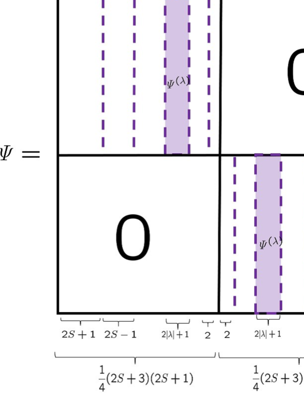
Figure 11: $\mathit{\Psi}$ (151) and $\tilde{\mathit{\Psi}}$ (155). (Left) For $\lambda>0$ ($\lambda<0$), $\mathit{\Psi}^{(\lambda)}$ appears in the up left (down right) block of $\mathit{\Psi}$. (Right) For $\lambda>0$ ($\lambda<0$), $\tilde{\mathit{\Psi}}^{(\lambda)}$ appears in the left (right) block of $\tilde{\mathit{\Psi}}$.

Rectangular matrices $\Psi^{(\lambda)}$ in Fig.11 are made of the $SO(4)$ monopole harmonics $\boldsymbol{\phi}_{\alpha}^{(\lambda)}\equiv\boldsymbol{\phi}_{\alpha}^{(s_{L},s_{R})=(\frac{S}{2}+\frac{1}{4}\text{sgn}(\lambda),\frac{S}{2}-\frac{1}{4}\text{sgn}(\lambda))}$ (350) as

$$\mathit{\Psi}^{(\lambda)}\equiv\begin{pmatrix}\mathit{\Psi}^{(\lambda)}_{1}&\mathit{\Psi}^{(\lambda)}_{2}&\cdots&\mathit{\Psi}^{(\lambda)}_{2|\lambda|+1}\end{pmatrix}=\begin{pmatrix}{\boldsymbol{\phi}_{1}^{(\lambda)}}^{\dagger}\\ {\boldsymbol{\phi}_{2}^{(\lambda)}}^{\dagger}\\ {\boldsymbol{\phi}_{3}^{(\lambda)}}^{\dagger}\\ \vdots\\ {\boldsymbol{\phi}_{(S+\frac{3}{2})(S+\frac{1}{2})}^{(\lambda)}}^{\dagger}\\ \end{pmatrix}.$$ (153)

See Fig.12 also.

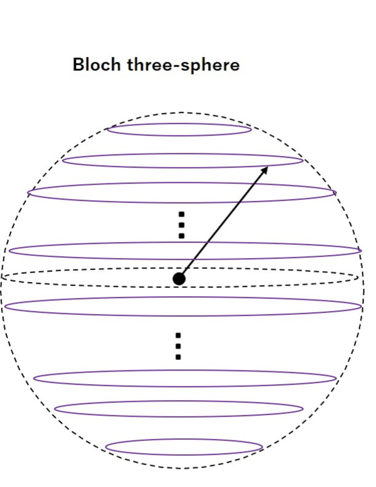
Figure 12: Bloch three-sphere and the $SO(4)$ Landau level eigenstates

With an appropriate unitary matrix $\mathcal{V}$, $\mathit{\Gamma}_{4}$ is diagonalized as in (147):

$$\mathcal{V}^{\dagger}\mathit{\Gamma}_{4}\mathcal{V}=\mathit{\Gamma}_{\text{diag}}.$$ (154)

Therefore, with

$$\tilde{\mathit{\Psi}}\equiv\mathit{\Psi}\mathcal{V},$$ (155)

we can diagonalize $H$ (148) as

$$\tilde{\mathit{\Psi}}^{\dagger}H\tilde{\mathit{\Psi}}=\frac{1}{2}\mathit{\Gamma}_{\text{diag}}=\begin{pmatrix}\frac{S}{2}\boldsymbol{1}_{2S+1}&0&0&0&0\\ 0&(\frac{S}{2}-\frac{1}{2})\boldsymbol{1}_{2S-1}&0&0&0\\ 0&0&(\frac{S}{2}-1)\boldsymbol{1}_{2S-3}&0&0\\ 0&0&0&\ddots&0\\ 0&0&0&0&-\frac{S}{2}\boldsymbol{1}_{2S+1}\end{pmatrix}+\frac{1}{4}G_{5}.$$ (156)

The eigenvalues rang from $-(\frac{S}{2}+\frac{1}{4})$ to $+\frac{S}{2}+\frac{1}{4}$, equally spaced by $1/2$, except for the spacing $1$ between $1/2$ and $-1/2$ (Fig.13).

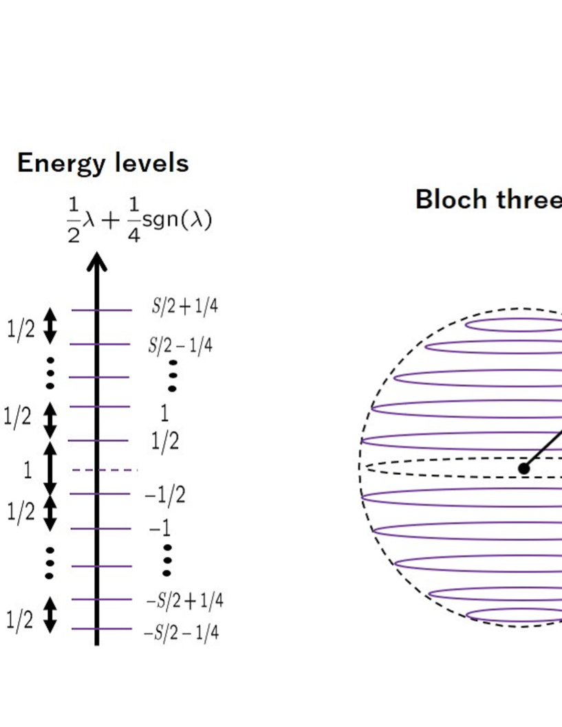
Figure 13: For odd $2S$, there are $2S+1$ energy levels. Note that zero-energy state is void.

The $SO(4)$ spin-coherent states ${\tilde{\mathit{\Psi}}^{(\lambda)}_{\sigma}}$ are realized in $\tilde{\mathit{\Psi}}$ as (Fig.11):

$$\tilde{\mathit{\Psi}} =\biggl{(}\tilde{\mathit{\Psi}}^{(S)}~{}\vdots~{}\tilde{\mathit{\Psi}}^{(S-1)})~{}\vdots~{}\cdots~{}\vdots~{}\tilde{\mathit{\Psi}}^{(1/2)}~{}\vdots~{}\tilde{\mathit{\Psi}}^{(-1/2)}~{}\vdots~{}\cdots~{}\vdots~{}\tilde{\mathit{\Psi}}^{(-S+1)}~{}\vdots~{}\mathit{\Psi}^{(-S)}\biggr{)}$$

$$=\biggl{(}\tilde{\mathit{\Psi}}^{(S)}_{S}\cdots\tilde{\mathit{\Psi}}^{(S)}_{-S}~{}\vdots~{}\tilde{\mathit{\Psi}}^{(S-1)}_{S-1}\cdots\tilde{\mathit{\Psi}}^{(S-1)}_{-(S-1)}~{}\vdots~{}\cdots~{}\vdots~{}\tilde{\mathit{\Psi}}^{(1/2)}_{1/2}~{}\tilde{\mathit{\Psi}}^{(1/2)}_{-1/2}~{}\vdots~{}\tilde{\mathit{\Psi}}^{(-1/2)}_{1/2}~{}\tilde{\mathit{\Psi}}^{(1/2)}_{-1/2}~{}\vdots~{}\cdots~{}\vdots~{}\tilde{\mathit{\Psi}}^{(-S+1)}_{S-1}\cdots\tilde{\mathit{\Psi}}^{(-S+1)}_{-(S-1)}~{}\vdots~{}\tilde{\mathit{\Psi}}^{(-S)}_{S}\cdots\tilde{\mathit{\Psi}}^{(-S)}_{-S}\biggr{)},$$ (157)

and they satisfy

$$H\tilde{\mathit{\Psi}}^{(\lambda)}_{\sigma}=\frac{1}{2}(\lambda+\frac{1}{2}\text{sgn}(\lambda))\cdot\tilde{\mathit{\Psi}}^{(\lambda)}_{\sigma}.~{}~{}(\sigma=\overbrace{|\lambda|,|\lambda|-1,|\lambda|-2,\cdots,-|\lambda|}^{=2|\lambda|+1})$$ (158)

Their ortho-normal relations are given by

$$({\tilde{\mathit{\Psi}}^{(\lambda)}_{\sigma}})^{\dagger}~{}{\tilde{\mathit{\Psi}}^{(\lambda^{\prime})}_{\tau}}=\delta_{\sigma\tau}\delta_{\lambda\lambda^{\prime}}.$$ (159)

Note that the energy levels of the $SO(5)$ and $SO(4)$ Zeeman-Dirac models are only equal for the $S=1/2$ case, but are generally distinct (compare Fig.13 with Fig.6). As the energy level approaches zero-energy by $1/2$, the degeneracy decreases by two, which leads to the absence of a zero-energy state (Fig.13). As usual, an $SO(3)$ gauge invariant quantity is given by the Bloch vector:

$$({\tilde{\mathit{\Psi}}}^{(\lambda)})^{\dagger}\mathit{\Gamma}_{\mu}{\tilde{\mathit{\Psi}}}^{(\lambda)}=(\lambda+\frac{1}{2}\text{sgn}(\lambda))\cdot x_{\mu}\boldsymbol{1}_{2|\lambda|+1}.$$ (160)

The quantum geometric tensor is a matrix-valued $SO(3)$ covariant quantity,

$$\chi^{(\lambda)}_{\theta_{i}\theta_{j}}\equiv\partial_{\theta_{i}}(\tilde{\mathit{\Psi}}^{(\lambda)})^{\dagger}\partial_{\theta_{j}}{\tilde{\mathit{\Psi}}^{(\lambda)}}-\partial_{\theta_{i}}(\tilde{\mathit{\Psi}}^{(\lambda)})^{\dagger}{\tilde{\mathit{\Psi}}^{(\lambda)}}~{}(\tilde{\mathit{\Psi}}^{(\lambda)})^{\dagger}\partial_{\theta_{j}}{\tilde{\mathit{\Psi}}^{(\lambda)}},~{}~{}~{}~{}(\theta_{i}=\chi,\theta,\phi)$$ (161)

and the trace of its symmetric part gives rise to the metric of three-sphere,

$$g^{(\lambda)}_{\theta_{i}\theta_{j}}=\frac{1}{2}\text{tr}(\chi^{(\lambda)}_{\theta_{i}\theta_{j}}+\chi^{(\lambda)}_{\theta_{j}\theta_{i}})~{}\propto~{}g_{\theta_{i}\theta_{j}}^{(S^{3})}=\text{diag}(1,~{}\sin^{2}\chi,~{}\sin^{2}\chi\sin^{2}\theta).$$ (162)

The proportional coefficients depend on both $S$ and $|\lambda|$. The Wilczek-Zee connection is derived as

$$-i\tilde{\mathit{\Psi}}^{\dagger}d\tilde{\mathit{\Psi}}={\mathcal{V}}^{\dagger}(-i\mathit{\Psi}^{\dagger}d\mathit{\Psi}){\mathcal{V}}=\left(\begin{array}[]{cccc:cccc}A^{(S)}&*&*&*&*&*&*&*\\ &A^{(S-1)}&*&*&*&*&*&*\\ &*&\ddots&*&*&*&*&*\\ &*&*&A^{(1/2)}&*&*&*&*\\ \hdashline*&*&*&*&A^{(-1/2)}&*&*&*\\ &*&*&*&*&\ddots&*&*\\ &*&*&*&*&*&A^{(-S+1)}&*\\ &*&*&*&*&*&*&A^{(-S)}\end{array}\right),$$ (163)

where

$$A^{(\lambda)}=-i(\tilde{\mathit{\Psi}}^{(\lambda)})^{\dagger}d\tilde{\mathit{\Psi}}^{(\lambda)}=-\frac{1}{1+x_{4}}\epsilon_{ijk}x_{j}S_{k}^{(|\lambda|)}dx_{i}=-i\frac{1}{2}({U^{(|\lambda|)}}^{\dagger}dU^{(|\lambda|)}+U^{(|\lambda|)}d{U^{(|\lambda|)}}^{\dagger})=A^{(-\lambda)},$$ (164)

with

$$U^{(|\lambda|)}\equiv e^{i\chi\sum_{i=1}^{3}y_{i}S_{i}^{(|\lambda|)}}.$$ (165)

Connection $A^{(\lambda)}$ (164) is represented as

$$A^{(\lambda)}=\frac{1}{2}\omega_{ij\theta_{k}}\epsilon_{ijk^{\prime}}S^{(|\lambda|)}_{k^{\prime}}d\theta_{k},$$ (166)

where $\omega_{ij\theta_{k}}$ denote the spin-connection of $S^{3}$. The corresponding curvature $F_{\theta_{i}\theta_{j}}=\partial_{\theta_{i}}A_{\theta_{j}}-\partial_{\theta_{j}}A_{\theta_{i}}+i[A_{\theta_{i}},A_{\theta_{j}}]$ is the antisymmetric part of (161):

$$F_{\theta_{i}\theta_{j}}^{(\lambda)}=-i(\chi_{\theta_{i}\theta_{j}}^{(\lambda)}-\chi_{\theta_{j}\theta_{i}}^{(\lambda)})=\frac{1}{2}e^{i^{\prime}}_{~{}\theta_{i}}\wedge e^{j^{\prime}}_{~{}\theta_{j}}\epsilon_{i^{\prime}j^{\prime}k^{\prime}}S_{k^{\prime}}^{(S)},$$ (167)

where $e^{i^{\prime}}_{~{}]\theta_{i}}$ denote the dreibein of $S^{3}$ [55].

5 Bloch hyper-spheres in even higher dimensions

This section discusses how the previous discussions are generalized in arbitrary dimensions. While $SO(d+1)$ large-spin gamma matrices can be derived in principle using the Landau level eigenstates of higher dimensional Landau models [83, 84, 85], their explicit evaluations will be a formidable task. We therefore deduce general results from a group theoretical analysis.

5.1 General properties

As discussed in the previous sections, the $SO(5)$ and $SO(4)$ Zeeman-Dirac models exhibit $SO(4)$ and $SO(3)$ symmetries, respectively. These symmetries introduce degeneracies in these models, and the associated Wilczek-Zee connections are described by the $SO(4)$ and $SO(3)$ monopole gauge fields. We will delve into how this concept is comprehended from a geometric perspective and can be extended to arbitrary dimensions. Let us consider the $SO(d+1)$ Zeeman-Dirac model

$$H=\sum_{a=1}^{d+1}x_{a}\cdot\frac{1}{2}\Gamma_{a},~{}~{}~{}~{}(\sum_{a=1}^{d+1}x_{a}x_{a}=1)$$ (168)

where $x_{a}$ are given parameters that denote the Bloch vector. In general, the $SO(d+1)$ Hamiltonian (168) has an $SO(d)$ symmetry,

$$U^{\dagger}HU=H.~{}~{}~{}~{}(U\in SO(d))$$ (169)

Each of the energy levels accommodates the degeneracy attributed to the $SO(d)$ symmetry. The geometric origin of this $SO(d)$ symmetry is explained as follows. Assume that $S_{ab}\in SO(d)$ denotes the rotation around the direction of the Bloch vector (Fig.14).

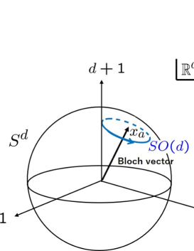
Figure 14: $SO(d)$ stabilizer group that does not transform the point $x_{a}$ (Bloch vector) on $S^{d}$.

Under such a transformation, the Bloch vector is apparently invariant

$$x_{a}~{}~{}~{}\rightarrow~{}~{}S_{ab}x_{b}=x_{a}.~{}~{}~{}~{}(S_{ab}\in SO(d))$$ (170)

Such a transformation that does not change a point on manifold is known as the stabilizer group. The $SO(d)$ stabilizer group appears as the denominator of the coset $S^{d}\simeq SO(d+1)/SO(d)$. The $SO(d)$ invariance of the Bloch vector can be reinterpreted as a symmetry of the Hamiltonian (168):

$$H=\sum_{a=1}^{d+1}x_{a}\cdot\frac{1}{2}\Gamma_{a}~{}~{}\rightarrow~{}~{}\sum_{a}(\sum_{b}S_{ab}x_{b})\cdot\frac{1}{2}\Gamma_{a}=\sum_{a}x_{a}\cdot\frac{1}{2}\overbrace{(\sum_{b}S_{ba}\Gamma_{a})}^{=U^{\dagger}\Gamma_{a}U}=U^{\dagger}HU.$$ (171)

Thus, the stabilizer group of the Bloch hyper-sphere guarantees the $SO(d)$ symmetry of the $SO(d+1)$ Zeeman-Dirac Hamiltonian. This $SO(d)$ symmetry introduces a corresponding degeneracy to each energy level. Next, let us clarify the geometric origin of the $SO(d)$ monopole gauge field. The adiabatic evolution of an $SO(d+1)$ spin-coherent state involves transitions among the degenerate states within each energy level. These transitions naturally give rise to the Wilczek-Zee connection. This Wilczek-Zee connection is attributed to the $SO(d)$ holonomy of $S^{d}$ and is identical to the gauge field of $SO(d)$ non-Abelian monopole. The above mechanics is summarized in Fig.15.

Figure 15: Emergence of the $SO(d)$ monopole gauge field from the $SO(d+1)$ Zeeman-Dirac model

In the following, we confirm these speculations through more concrete analyses.

5.2 $SO(2k+1)$ and $SO(2k)$ Representations

Before proceeding to details, we present a general argument about the representations of the orthogonal groups. Assume that $[l_{1},l_{2},\cdots,l_{k}]_{SO(2k+1)}$ and $[l_{1},l_{2},\cdots,l_{k}]_{SO(2k)}$ signify the Young tableaux of the $SO(2k+1)$ and $SO(2k)$ groups, respectively [86]. The representations of our interest are designated as

$$[\lambda]_{SO(2k+1)}\equiv[S,\lambda]_{SO(2k+1)}\equiv[\overbrace{S,S,\cdots,S,\lambda}^{k}]_{SO(2k+1)}~{}~{}~{}~{}(0\leq\lambda\leq S),$$ (174)

$$[\lambda]_{SO(2k)}\equiv[S,\lambda]_{SO(2k)}\equiv[\overbrace{S,S,\cdots,S,\lambda}^{k}]_{SO(2k)}~{}~{}~{}~{}(-S\leq\lambda\leq S),$$ (175)

with dimensions being

$$D_{SO(2k+1)}(\lambda)\equiv D_{SO(2k+1)}(S,\lambda)\equiv\frac{2\lambda+1}{2S+1}\prod_{j=1}^{k-1}\frac{S-\lambda+k-j}{k-j}\frac{S+\lambda+k-j+1}{2S+k-j+1}\cdot\prod_{l=1}^{k}\prod_{i=1}^{l}\frac{2S+l+i-1}{l+i-1},$$ (176a)

$$D_{SO(2k)}(\lambda)\equiv D_{SO(2k)}(S,\lambda)\equiv\prod_{j=1}^{k-1}\frac{(S+j)^{2}-\lambda^{2}}{j^{2}}~{}\cdot~{}\prod_{l=1}^{k-2}\prod_{i=1}^{k-l-1}\frac{2S+2l+i}{2l+i}=D_{SO(2k)}(-\lambda).$$ (176b)

In particular,

$$D_{SO(2k+1)}(S)=D_{SO(2k+2)}(\pm S)=\prod_{l=1}^{k}\prod_{i=1}^{l}\frac{2S+l+i-1}{l+i-1}~{}~{}\sim~{}~{}S^{\frac{1}{2}k(k+1)}~{}\sim~{}S\cdot D_{SO(2k)(1/2)}=S^{1},S^{3},S^{6},S^{10},\cdots,$$ (179a)

$$D_{SO(2k)}(1/2)=D_{SO(2k)}(-1/2)=\prod_{j=1}^{k-1}\frac{(2S+2j)^{2}-1}{(2j)^{2}}~{}\cdot~{}\prod_{l=1}^{k-2}\prod_{i=1}^{k-l-1}\frac{2S+2l+i}{2l+i}~{}~{}\sim~{}~{}S^{\frac{1}{2}(k+2)(k-1)}=S^{0},S^{2},S^{5},S^{9},\cdots.$$ (179b)

As we shall see in Secs.5.3 and 5.4, $D_{SO(2k+1)}(\lambda)/D_{SO(2k)}(\lambda)$ indicates the degeneracy of the energy level indexed by $\lambda$ of the $SO(2k+2)/SO(2k+1)$ model. The degeneracies (176) are depicted in Fig.16.

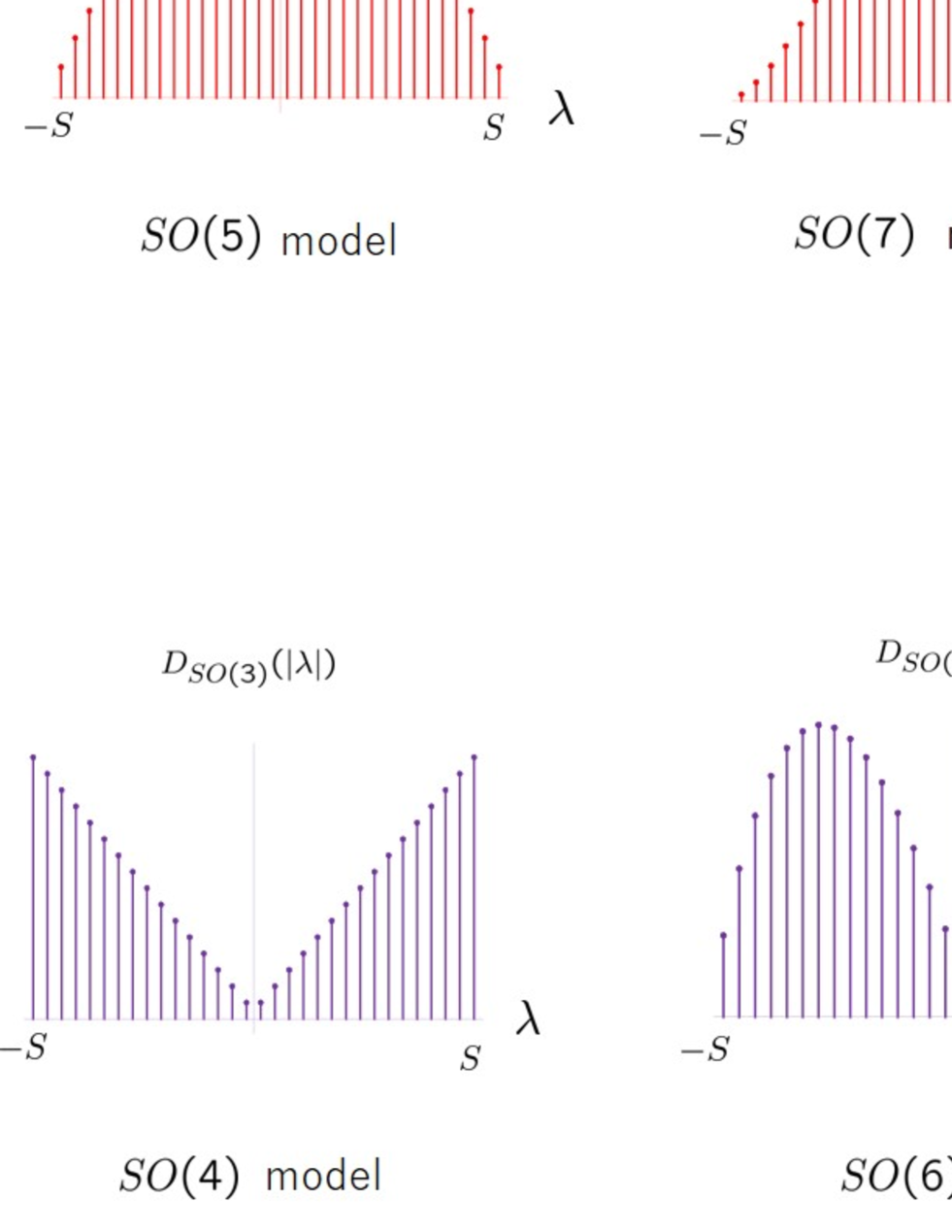
Figure 16: The upper/lower figure represents the distributions of the degeneracies of the $SO(2k+1)$/$SO(2k)$ Zeeman-Dirac model for $2S=31$.

There are interesting relations between adjacent dimensions:

$$D_{SO(2k+1)}(S)=\sum_{\lambda=-S}^{S}D_{SO(2k)}(\lambda),$$ (180a)

$$D_{SO(2k)}(1/2)=\sum_{\lambda=\frac{1}{2}}^{S}D_{SO(2k-1)}(\lambda)=\sum_{\lambda=-S}^{-\frac{1}{2}}D_{SO(2k-1)}(-\lambda)=D_{SO(2k)}(-1/2).~{}~{}~{}~{}(2S~{}:~{}\text{odd}),$$ (180b)

which imply

$$\Sigma_{\mu\nu}^{[S]_{SO(2k+1)}}=\bigoplus_{\lambda=-S}^{S}\Sigma_{\mu\nu}^{[\lambda]_{SO(2k)}}~{}~{}~{}(\mu,\nu=1,2,\cdots,2k),$$ (181a)

$$\Sigma_{ij}^{[1/2]_{SO(2k)}}=\bigoplus_{\lambda=1/2}^{S}\Sigma_{ij}^{[\lambda]_{SO(2k-1)}}~{}~{}(i,j=1,2,\cdots,2k-1).$$ (181b)

Notice that (180b) holds $\it{only}$ for odd $2S$, not for even $2S$. (Recall that odd dimensional Bloch hyper-spheres are defined only for half-integer $S$.) Equation (180) implies the dimensional hierarchies between even and odd dimensions.

5.3 $SO(2k+1)$ Zeeman-Dirac model

As in the $SO(5)$ case, there exist large spin gamma matrices for arbitrary $SO(2k+1)$ groups (see Refs.[87, 88] as reviews and references therein). Using such gamma matrices, we can construct the large spin $SO(2k+1)$ Zeeman-Dirac model. For a better understanding, we analyze the $SO(2k+1)$ minimal model in Appendix E.2.

The $SO(2k+1)$ large spin gamma matrices satisfy two basic equations

$$\sum_{a=1}^{2k+1}\Gamma_{a}\Gamma_{a}=4S(S+k)\boldsymbol{1}_{D_{SO(2k+1)}(S)},$$ (183a)

$$[\Gamma_{a_{1}},\Gamma_{a_{2}},\cdots,\Gamma_{a_{2k}}]=i^{k}\frac{(2k)!!~{}(2S+2k-2)!!}{(2S)!!}~{}\epsilon_{a_{1}a_{2}\cdots a_{2k+1}}\Gamma_{a_{2k+1}},$$ (183b)

where $[~{},~{},\cdots,~{}]$ is called the $2k$-bracket that signifies totally antisymmetric combination of the $2k$ quantities inside the bracket. Matrices $\Gamma_{a}$ thus satisfy the quantum Nambu geometry [89, 90] and act as the coordinates of fuzzy $2k$-sphere. The commutators between $\Gamma_{a}$s yield the $SO(2k+1)$ generators of symmetric representation

$$\Sigma_{ab}^{[S]_{SO(2k+1)}}=-i\frac{1}{4}[\Gamma_{a},\Gamma_{b}].$$ (185)

The $SO(2k+1)$ covariance of $\Gamma_{a}$ is represented as $[\Sigma_{ab}^{[S]_{SO(2k+1)}},\Gamma_{c}]=i\delta_{ac}\Gamma_{b}-i\delta_{bc}\Gamma_{a}$. The $SO(2k+1)$ Zeeman-Dirac Hamiltonian

$$H=\sum_{a=1}^{2k+1}x_{a}\cdot\frac{1}{2}\Gamma_{a}~{}~{}~{}~{}~{}~{}(\sum_{a=1}^{2k+1}x_{a}x_{a}=1)$$ (186)

is diagonalized as

$$\Psi^{\dagger}H\Psi=\frac{1}{2}\Gamma_{2k+1}=\bigoplus_{\lambda=-S}^{S}~{}\lambda~{}\boldsymbol{1}_{D_{SO(2k)}(\lambda)},$$ (187)

where

$$\Psi=e^{i\theta_{2k}\sum_{\mu=1}^{2k}y_{\mu}\Sigma_{\mu,{2k+1}}^{[S]_{SO(2k+1)}}}=N^{\dagger}\cdot e^{i\theta_{2k}\Sigma_{2k,2k+1}^{[S]_{SO(2k+1)}}}\cdot N,~{}~{}~{}~{}~{}(y_{\mu=1,2,\cdots,2k}=\frac{1}{\sin\theta_{2k}}x_{\mu},~{}~{}~{}x_{2k+1}=\cos\theta_{2k})$$ (188)

with

$$N=e^{i\theta_{2k-1}\Sigma_{2k,2k-1}^{[S]_{SO(2k+1)}}}~{}e^{i\theta_{2k-2}\Sigma_{2k-1,2k-2}^{[S]_{SO(2k+1)}}}~{}\cdots~{}e^{i\theta_{4}\Sigma_{54}^{[S]_{SO(2k+1)}}}~{}e^{i\theta_{3}\Sigma_{43}^{[S]_{SO(2k+1)}}}~{}e^{i\theta\Sigma_{31}^{[S]_{SO(2k+1)}}}~{}e^{i\phi\Sigma_{12}^{[S]_{SO(2k+1)}}}.$$ (189)

As shown in (187), the $SO(2k+1)$ Hamiltonian exhibits $2S+1$ energy levels

$$\lambda=S,~{}S-1,~{}S-2,\cdots,-S,$$ (190)

with degeneracies $D_{SO(2k)}(\lambda)$ (176b). The spectrum (190) is symmetric with respect to the origin, and the geometric picture of the Bloch $2k$-sphere is similar to that of the Bloch four-sphere (Fig.6), up to energy level degeneracy.

This $SO(2k)$ degeneracy comes from the $SO(2k)$ symmetry of (187)

$$\Psi~{}\rightarrow~{}\Psi\cdot e^{i\frac{1}{2}\omega_{\mu\nu}\Sigma^{[S]_{SO(2k+1)}}_{\mu\nu}}.$$ (191)

The $SO(2k)$ decomposition (180a) and the analyses of Appendix E.2 suggest that the Wilczek-Zee $SO(2k)$ connection is given by the $SO(2k)$ monopole gauge field,

$$A^{(\lambda)}=-\frac{1}{1+x_{2k+1}}\Sigma_{\mu\nu}^{[\lambda]_{SO(2k)}}x_{\nu}dx_{\mu},$$ (192)

where $\Sigma_{\mu\nu}^{[\lambda]_{SO(2k)}}$ denote the $SO(2k)$ generators of $[\lambda]_{SO(2k)}$. We explicitly checked the validity of (192) using generalized $SO(7)$ gamma matrices for $S=1/2,1,3/2$ . The non-trivial topology of $SO(2k)$ monopole field configuration is specified by the $k$th Chern number

$$\text{ch}_{k}=\frac{1}{k!(2\pi)^{k}}\int_{S^{2k}}\text{tr}(F^{k}),$$ (193)

which is equivalent to the homotopy map from the equator to the $SO(2k)$ transition function,

$$\pi_{2k-1}(SO(2k))~{}\simeq~{}\mathbb{Z}.$$ (194)

For the monopole configuration (192), the $k$th Chern number is evaluated as

$$\text{ch}_{k}^{[\lambda]_{SO(2k)}}=\text{sgn}(\lambda)\cdot D_{SO(2k+1)}(S-\frac{1}{2},|\lambda|-\frac{1}{2})=-\text{ch}_{k}^{[-\lambda]_{SO(2k)}}$$ (195)

with $\text{sgn}(0)\equiv 0$. Equation (195) is an apparent generalization of the previous $k=2$ case (115). Two opposite energy levels with respect to the zero-energy have the same magnitude of Chern numbers with opposite signs.

5.4 $SO(2k)$ Zeeman-Dirac model

The $SO(2k)$ large-spin gamma matrices are realized in the subspace $\lambda=(+1/2)\oplus(-1/2$) of the $SO(2k+1)$ large-spin gamma matrices [80, 82]. The spin magnitude $S$ should be a half-integer for the same reason as in the $SO(4)$ models. An analysis of the $SO(2k)$ minimal Zeeman-Dirac model is presented in Appendix E.3.

The $SO(2k)$ large spin gamma matrices are given by the off-diagonal block matrices,

$$\mathit{\Gamma}_{\mu}=\begin{pmatrix}0&\mathcal{Y}_{\mu}^{\dagger}\\ \mathcal{Y}_{\mu}&0\end{pmatrix}.~{}~{}~{}~{}~{}~{}(\mu=1,2,\cdots,2k)$$ (196)

They satisfy the following two equations:

$$\sum_{\mu=1}^{2k}\mathit{\Gamma}_{\mu}\mathit{\Gamma}_{\mu}=\frac{1}{2}(2S+1)(2S+2k-1)\boldsymbol{1}_{2D_{SO(2k)}(1/2)},$$ (200a)

$$[\![\mathit{\Gamma}_{\mu_{1}},\mathit{\Gamma}_{\mu_{2}},\cdots,\mathit{\Gamma}_{\mu_{2k-1}}]\!]=-i^{k}~{}\frac{(2k)!!~{}(2S+2k-2)!!}{(2S)!!}~{}\epsilon_{\mu_{1}\mu_{2}\cdots\mu_{2k}}\mathit{\Gamma}_{\mu_{2k}},$$ (200b)

where

$$[\![\mathit{\Gamma}_{\mu_{1}},\mathit{\Gamma}_{\mu_{2}},\cdots,\mathit{\Gamma}_{\mu_{2k-1}}]\!]\equiv[\mathit{\Gamma}_{\mu_{1}},\mathit{\Gamma}_{\mu_{2}},\cdots,\mathit{\Gamma}_{\mu_{2k-1}},G_{{2k+1}}]=2k~{}[\mathit{\Gamma}_{\mu_{1}},\mathit{\Gamma}_{\mu_{2}},\cdots,\mathit{\Gamma}_{\mu_{2k-1}}]G_{{2k+1}}.$$ (201)

Eq.(200a) was derived in Ref.[80]. Matrix $G_{5}$ is a diagonal matrix

$$G_{2k+1}=\begin{pmatrix}\boldsymbol{1}_{D_{SO(2k)}(1/2)}&0\\ 0&-\boldsymbol{1}_{D_{SO(2k)}(1/2)}\end{pmatrix},$$ (202)

which anti-commutes with all $\mathit{\Gamma}_{\mu}$s:

$$\{\mathit{\Gamma}_{\mu},G_{2k+1}\}=0.$$ (203)

With such $\mathit{\Gamma}_{\mu}$, we construct the $SO(2k)$ Zeeman-Dirac Hamiltonian as

$${H}=\sum_{\mu=1}^{2k}x_{\mu}\cdot\frac{1}{2}\mathit{\Gamma}_{\mu}=\frac{1}{2}\begin{pmatrix}0&\mathit{Q}^{(-)}\\ \mathit{Q}^{(+)}&0\end{pmatrix}~{}~{}~{}~{}~{}~{}(\sum_{\mu=1}^{2k}x_{\mu}x_{\mu}=1),$$ (204)

where

$$\mathit{Q}^{(+)}\equiv\sum_{\mu=1}^{2k}x_{\mu}\mathcal{Y}_{\mu},~{}~{}~{}~{}\mathit{Q}^{(-)}\equiv{\mathit{Q}^{(+)}}^{\dagger}=\sum_{\mu=1}^{2k}x_{\mu}\mathcal{Y}_{\mu}^{\dagger}.$$ (205)

Hamiltonian (204) apparently has the chiral symmetry:

$$\{\mathit{H},G_{2k+1}\}=0.$$ (206)

While the commutators between $\mathit{\Gamma}_{\mu}$s do not realize $SO(2k)$ generators, $\mathit{\Gamma}_{\mu}$ transform as a vector under the $SO(2k)$ transformations generated by the following $SO(2k)$ generators [64],

$$\mathit{\Sigma}_{\mu\nu}\equiv\begin{pmatrix}\Sigma_{\mu\nu}^{[+1/2]_{SO(2k)}}&0\\ 0&\Sigma_{\mu\nu}^{[-1/2]_{SO(2k)}}\end{pmatrix}.$$ (207)

The non-linear realization matrix is constructed as

$$\mathit{\Psi}=e^{i\theta_{2k-1}\sum_{i=1}^{2k-1}y_{i}\mathit{\Sigma}_{i,{2k}}}=\mathcal{N}^{\dagger}~{}e^{i\theta_{2k-1}\mathit{\Sigma}_{2k-1,2k}}~{}\mathcal{N}=\begin{pmatrix}\mathcal{U}^{[+1/2]}&0\\ 0&\mathcal{U}^{[-1/2]}\end{pmatrix},$$ (208)

where

$$y_{i=1,2,\cdots,2k-1}=\frac{1}{\sin(\theta_{2k-1})}x_{i}~{}~{}~{}x_{2k}=\cos(\theta_{2k-1}),$$ (209a)

$$\mathcal{N}=e^{i\theta_{2k-2}\mathit{\Sigma}_{2k-1,2k-2}}e^{i\theta_{2k-3}\mathit{\Sigma}_{2k-2,2k-3}}\cdots e^{i\theta_{4}\mathit{\Sigma}_{54}}e^{i\theta_{3}\mathit{\Sigma}_{43}}e^{i\theta\mathit{\Sigma}_{31}}e^{i\phi\mathit{\Sigma}_{12}},$$ (209b)

$$\mathcal{U}^{[\pm 1/2]}\equiv e^{i\theta_{2k-1}\sum_{i=1}^{2k-1}y_{i}{\Sigma}^{[\pm 1/2]_{SO(2k)}}_{i,{2k}}}.$$ (209c)

Matrix $\mathit{\Psi}$ transforms the $SO(2k)$ Hamiltonian (204) into the form

$$\mathit{\Psi}^{\dagger}{H}\mathit{\Psi}=\frac{1}{2}\mathit{\Gamma}_{2k}.$$ (210)

With an appropriate unitary matrix $\mathcal{V}$, $\mathit{\Gamma}_{2k}$ is diagonalized as

$$\mathcal{V}^{\dagger}\mathit{\Gamma}_{2k}\mathcal{V}=\mathit{\Gamma}_{\text{diag}}\equiv{\bigoplus_{\lambda=-S}^{S}}~{}(\lambda+\frac{1}{2}\text{sgn}(\lambda))~{}\boldsymbol{1}_{D_{SO(2k-1)}(|\lambda|)}={\bigoplus_{\lambda=-S}^{S}}~{}\lambda~{}\boldsymbol{1}_{D_{SO(2k-1)}(|\lambda|)}+\frac{1}{2}G_{2k+1}.$$ (211)

Hence, with $\tilde{\mathit{\Psi}}=\mathit{\Psi}\mathcal{V}$, we can diagonalize the Hamiltonian as

$$\tilde{\mathit{\Psi}}^{\dagger}{H}\tilde{\mathit{\Psi}}=\frac{1}{2}\mathit{\Gamma}_{\text{diag}}={\bigoplus_{\lambda=-S}^{S}}~{}\frac{1}{2}(\lambda+\frac{1}{2}\text{sgn}(\lambda))~{}\boldsymbol{1}_{D_{SO(2k-1)}(|\lambda|)}.$$ (212)

There apparently exist $SO(2k-1)$ degrees of freedom in (210):

$$\mathit{\Psi}~{}~{}\rightarrow~{}~{}\mathit{\Psi}\cdot e^{i\frac{1}{2}\sum_{i,j=1}^{2k-1}\omega_{ij}\mathit{\Sigma}_{ij}}$$ (213)

or

$$\tilde{\mathit{\Psi}}~{}~{}\rightarrow~{}~{}\tilde{\mathit{\Psi}}\cdot e^{i\frac{1}{2}\sum_{i,j=1}^{2k-1}\omega_{ij}\tilde{\mathit{\Sigma}}_{ij}}.~{}~{}~{}~{}~{}~{}~{}(\tilde{\mathit{\Sigma}}_{ij}\equiv\mathcal{V}^{\dagger}\mathit{\Sigma}_{ij}\mathcal{V})$$ (214)

For a Hamiltonian with chiral symmetry, we can define the winding number [46]

$$\nu^{(\pm)}\equiv(-i)^{k-1}\frac{1}{(2\pi)^{k}}\frac{(k-1)!}{(2k-1)!}\int_{S^{2k-1}}\text{tr}((-i\mathit{Q}^{(\mp)}d\mathit{Q}^{(\pm)})^{2k-1})=\pm D_{SO(2k+1)}(S-\frac{1}{2},0)=\text{ch}_{k}^{[\pm\frac{1}{2}]_{SO(2k)}},$$ (215)

which corresponds to the homotopy map

$$\pi_{2k-1}(SO(2k))~{}\simeq~{}\mathbb{Z}.$$ (216)

The diagonal blocks of $-i\tilde{\mathit{\Psi}}^{\dagger}d\tilde{\mathit{\Psi}}$ may yield the $SO(2k-1)$ Wilczek-Zee connection in a similar fashion to (163):

$$A^{(\lambda)}=-\frac{1}{1+x_{2k}}\Sigma_{ij}^{[|\lambda|]_{SO(2k-1)}}x_{j}dx_{i}.$$ (217)

This result is consistent with the analysis of the $SO(2k)$ spinor representation (Appendix E.3) and the $SO(2k-1)$ decomposition (180b).

We pictorially depict the obtained results in Fig.17.

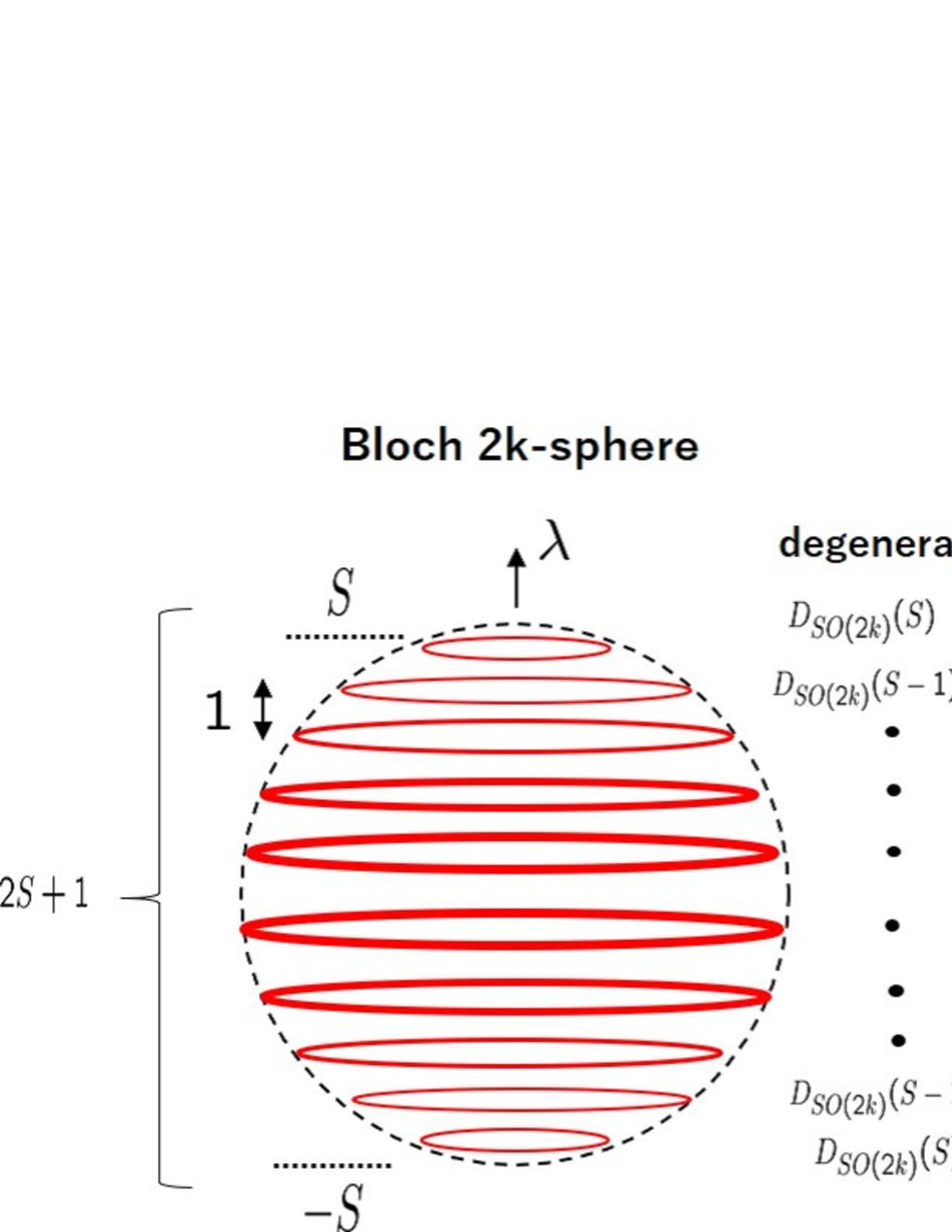
Figure 17: The Bloch $2k$-sphere (left) and the Bloch $(2k-1)$-sphere (right). There are $2S+1$ energy levels in either case. For the Bloch $2k$-spheres, the degeneracies increase toward the equator: As $k$ increases, the peak on the equator becomes shaper (see the upper figures of Fig.16 also). For the Bloch $(2k-1)$-spheres, the degeneracies have two peaks in the northern and southern hemispheres: As $k$ increases, the two peaks approach the equator (see the lower figures of Fig.16 also.)

6 Bloch hyper-balls and quantum statistics

We refer to the $d+1$ dimensional hyper-volume region surrounded by the Bloch hyper-sphere $S^{d}$ as the Bloch hyper-ball, $B^{d+1}$. Here, we consider $2S+1$-level density matrices whose parameters are given by the coordinates of $B^{d+1}$ and investigate the corresponding von Neumann entropies and the Bures information metrics.

6.1 Bloch hyper-balls and density matrices

Arbitrary $2\times 2$ density matrix is represented as

$$\rho=\frac{1}{2}(\boldsymbol{1}_{2}+r\sum_{i=1}^{3}x_{i}\sigma_{i}),~{}~{}~{}~{}(0\leq r\leq 1,~{}~{}~{}{\sum_{i=1}^{3}x_{i}x_{i}}=1)$$ (218)

which is formally equivalent to

$$\rho=\frac{1}{2}\boldsymbol{1}_{2}+rH.$$ (219)

Here, $H$ denotes the $SO(3)$ Zeeman-Dirac Hamiltonian (4). The parameters $rx_{i}$ indicate a position inside the Bloch three-ball to specify the density matrix (218).

In the following, we explore the density matrix made of the $SO(d+1)$ Zeeman-Dirac Hamiltonian $H$:

$$\rho=\alpha\boldsymbol{1}+\beta H,$$ (220)

where $\alpha$ and $\beta$ are quantities to be determined so that $\rho$ satisfies the necessary conditions for density matrix:

$$1.~{}\text{$\rho$ is Hermitian}~{}~{}~{}~{}~{}~{}2.~{}\text{ $\text{tr}(\rho)=1$}~{}~{}~{}~{}~{}~{}~{}3.~{}\text{The eigenvalues of $\rho$ are non-negative}.$$

The first condition implies that $\alpha$ and $\beta$ should be real parameters. The second condition determines $\alpha=\frac{1}{\text{tr}\boldsymbol{1}}$, provided $H$ is a traceless matrix as in the present case. The third condition determines $0\leq\beta\leq\alpha/(h_{1}\equiv\text{Max}(\text{eigenvalues of}~{}H))$ when the spectrum of $H$ is symmetric with respective to the zero-energy as in the present case. Consequently, we have

$$\alpha=\frac{1}{\text{tr}\boldsymbol{1}},~{}~{}~{}~{}~{}~{}~{}\beta=\frac{\alpha}{h_{1}}r,~{}~{}~{}~{}~{}(0\leq r\leq 1)$$ (221)

and (220) becomes

$$\rho=\frac{1}{\text{tr}\boldsymbol{1}}(\boldsymbol{1}+\frac{1}{h_{1}}rH).$$ (222)

The present density matrix represents a special multi-level density matrix. For the parameter region of a general multi-level density matrix, one can consult with [28, 29]. The geometry of the allowed region is much more intricate than the simple volume region of hyper-ball.

For the case of the $SO(2k+1)$ model, the parameters are identified as $\alpha=D_{SO(2k+1)}(S)$ and $h_{1}=S$. Therefore, the density matrix becomes

$$\rho=\frac{1}{D_{SO(2k+1)}(S)}\biggl{(}\boldsymbol{1}_{D_{SO(2k+1)}(S)}+r\frac{1}{S}\sum_{a=1}^{2k+1}x_{a}\cdot\frac{1}{2}\Gamma_{a}\biggr{)}~{}~{}~{}~{}~{}~{}~{}~{}(0\leq r\leq 1,~{}~{}~{}{\sum_{a=1}^{2k+1}x_{a}x_{a}}=1).$$ (223)

The condition $0\leq r\leq 1$ indicates the occupied region by the Bloch $2k+1$-ball, and the density matrix is defined at each point inside the $B^{2k+1}$.

Similarly for the $SO(2k)$ model case, the parameters are identified as $\alpha=2D_{SO(2k)}(1/2)$ and $h_{1}=\frac{1}{2}(S+\frac{1}{2})$. The density matrix is then given by

$$\rho=\frac{1}{2D_{SO(2k)}(1/2)}\biggl{(}\boldsymbol{1}_{2D_{SO(2k)}(1/2)}+r\frac{4}{2S+1}\sum_{\mu=1}^{2k}x_{\mu}\cdot\frac{1}{2}\mathit{\Gamma}_{\mu}\biggr{)}~{}~{}~{}~{}~{}(2S:\text{odd},~{}~{}~{}0\leq r\leq 1,~{}~{}~{}{\sum_{\mu=1}^{2k}x_{\mu}x_{\mu}}=1).$$ (224)

6.2 Bloch hyper-balls and von Neumann entropies

With a given density matrix $\rho$, the von Neumann entropy is defined as

$$S_{vN}=-\text{tr}(\rho\ln\rho)=-\sum_{\lambda}D(\lambda)~{}\rho_{\lambda}\ln\rho_{\lambda},~{}~{}~{}~{}(\text{tr}\rho=\sum_{\lambda}D(\lambda)~{}\rho_{\lambda}=1)$$ (225)

where $\rho_{\lambda}$ denote the eigenvalues of $\rho$ with degeneracy $D(\lambda)$. For the present models,

$$B^{2k+1}~{}~{}:~{}\rho_{\lambda}(r)=\frac{1}{D_{SO(2k+1)}(S)}\biggl{(}1+\frac{\lambda}{S}r\biggr{)},~{}~{}~{}~{}D(\lambda)=D_{SO(2k)}(\lambda),$$ (226a)

$$B^{2k}~{}~{}:~{}\rho_{\lambda}(r)=\frac{1}{2D_{SO(2k)}(1/2)}\biggl{(}1+\frac{2\lambda+\text{sgn}(\lambda)}{2S+1}r\biggr{)},~{}~{}~{}~{}D(\lambda)=D_{SO(2k-1)}(|\lambda|).$$ (226b)

Using (180), we can readily confirm that (226) satisfies $\text{tr}\rho=\sum_{\lambda=-S}^{S}D(\lambda)\rho_{\lambda}(r)=1$. Their von Neumann entropies (225) are evaluated as

$$B^{2k+1}:~{}S_{vN}(r) =\ln(D_{SO(2k+1)}(S))-\frac{1}{D_{SO(2k+1)}(S)}\sum_{\lambda=-S}^{S}D_{SO(2k)}(\lambda)\cdot(1+\frac{\lambda}{S}r)\cdot\ln(1+\frac{\lambda}{S}r),$$ (227a)

$$B^{2k}:~{}S_{vN}(r) =\ln(2D_{SO(2k)}(1/2))$$

$$-\frac{1}{2D_{SO(2k)}(1/2)}\sum_{\lambda=-S}^{S}D_{SO(2k-1)}(|\lambda|)\cdot(1+\frac{2\lambda+\text{sgn}(\lambda)}{2S+1}r)\cdot\ln(1+\frac{2\lambda+\text{sgn}(\lambda)}{2S+1}r),$$ (227b)

where we used (180) again. The core of the Bloch hyper-ball ($r=0$) signifies the maximally mixed ensemble:

$$\rho=\frac{1}{N}\boldsymbol{1}_{N},~{}~{}\text{Max}(S_{vN})=\ln N.~{}~{}~{}(N=D_{SO(2k+1)(S)},~{}~{}2D_{SO(2k)(1/2)})$$ (228)

The von Neumann entropy (227) monotonically decreases as $r$ increases regardless of the parity of dimensions (see the left of Fig.18).

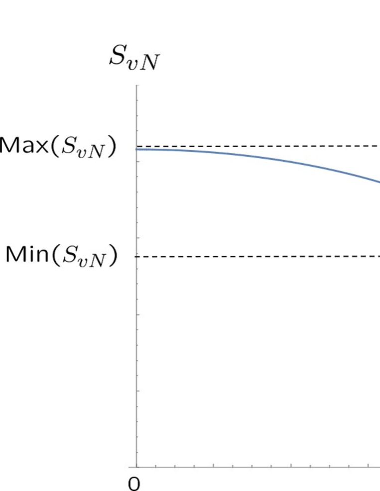
Figure 18: (Left) General behavior of the von Neumann entropy for a Bloch hyper-ball. (Right) The von Neumann entropies for the minimal Bloch $d+1$-balls $(k=[(d+1)/2]).$

For the Bloch balls of minimal spin $S=1/2$, the density matrices are given by

$$B^{2k+1}~{}:~{}\rho|_{S=1/2}=\frac{1}{2^{k}}(\boldsymbol{1}_{2^{k}}+r\sum_{a=1}^{2k+1}x_{a}\gamma_{a}),~{}~{}~{}~{}~{}~{}~{}~{}~{}~{}~{}B^{2k}~{}:~{}\rho|_{S=1/2}=\frac{1}{2^{k}}(\boldsymbol{1}_{2^{k}}+r\sum_{\mu=1}^{2k}x_{\mu}\gamma_{\mu}),$$ (229)

both of which are diagonalized as

$$\rho|_{S=1/2}\rightarrow\frac{1}{2^{k}}\begin{pmatrix}(1+r)\boldsymbol{1}_{2^{k-1}}&0\\ 0&(1-r)\boldsymbol{1}_{2^{k-1}}\end{pmatrix},$$ (230)

and so the von Neumann entropies for $B^{2k+1}$ and $B^{2k}$ take the same value (see the right of Fig.18),

$$S_{vN}(r)|_{S=1/2}=k\ln 2-\frac{1}{2}(1+r)\ln(1+r)-\frac{1}{2}(1-r)\ln(1-r).$$ (231)

Their maximum value and minimum value are respectively given by

$$\text{Max}(S_{vN})|_{S=1/2}=S_{vN}(0)|_{S=1/2}=k\ln 2,~{}~{}~{}~{}~{}\text{Min}(S_{vN})|_{S=1/2}=S_{vN}(0)|_{S=1/2}=(k-1)\ln 2.$$ (232)

The maximum value $\ln(2^{k})$ is accounted for by the $2^{k}$ matrix dimension of the $SO(2k+1)$/$SO(2k)$ minimal Hamiltonian, while the minimum value $\ln(2^{k-1})$ comes from the $2^{k-1}$ degeneracy of the energy level of the Hamiltonian.

6.3 Quantum statistical geometry

We will discuss quantum statistical geometries. First let us investigate the trace distance between the density matrices, $L\equiv\frac{1}{2}\text{tr}(\sqrt{(\rho-\rho^{\prime})^{2}})$. From (226), the trace distance is readily derived as

$$L=c(S,d+1)\cdot\sqrt{\sum_{\alpha=1}^{d+1}(rx_{\alpha}-r^{\prime}x^{\prime}_{\alpha})^{2}},$$ (233)

where

$$c(S,2k+1)\equiv\sum_{\lambda=-S}^{S}\frac{|\lambda|}{4S}\frac{D_{SO(2k)}(\lambda)}{D_{SO(2k+1)}(S)},~{}~{}~{}~{}~{}c(S,2k)\equiv\sum_{\lambda=1/2}^{S}\frac{2\lambda+1}{2S+1}\frac{D_{SO(2k-1)}(\lambda)}{D_{SO(2k)}(1/2)}.$$ (234)

In particular for $S=1/2$, $c$s (234) do not depend on $k$, $c(1/2,2k+1)=1/4$ and $c^{\prime}(1/2,2k)=1$. Generally, $c$s monotonically decrease as $S$ and $k$ increase. The trace distance (233) is proportional to the distance between the vectors $rx_{\alpha}$ and ${}^{\prime}x^{\prime}_{\alpha}$ in the $d+1$ dimensional flat Euclidean space.

Next, we will derive Bures metric [91, 92]. $SO(d+1)$ rotationally symmetric curved spaces emerge as the Bures geometries. From the formula of [93], we can evaluate the Bures metrics

$$B^{2k+1}~{}:~{}B_{ab}=\sum_{\lambda,\lambda^{\prime}=-S}^{S}\frac{1}{2(\rho_{\lambda}+\rho_{\lambda^{\prime}})}\text{tr}\biggl{(}{\Psi^{(\lambda)}}^{\dagger}\frac{\partial\rho}{\partial X_{a}}\Psi^{(\lambda^{\prime})}~{}{\Psi^{(\lambda^{\prime})}}^{\dagger}\frac{\partial\rho}{\partial X_{b}}{\Psi^{(\lambda)}}\biggr{)},$$ (235a)

$$B^{2k}~{}~{}~{}:~{}B_{\mu\nu}=\sum_{\lambda,\lambda^{\prime}=-S}^{S}\frac{1}{2(\rho_{\lambda}+\rho_{\lambda^{\prime}})}\text{tr}\biggl{(}(\tilde{\mathit{\Psi}}^{(\lambda)})^{\dagger}\frac{\partial\rho}{\partial X_{\mu}}\tilde{\mathit{\Psi}}^{(\lambda^{\prime})}~{}(\tilde{\mathit{\Psi}}^{(\lambda^{\prime})})^{\dagger}\frac{\partial\rho}{\partial X_{\nu}}{\tilde{\mathit{\Psi}}^{(\lambda)}}\biggr{)}.$$ (235b)

While the Bures metrics (235) may take various forms depending on the functional forms of the spin-coherent states, they generally take the $SO(d+1)$ spherical symmetric form

$$B_{\alpha\beta}=f(r)\delta_{\alpha\beta}+g(r)x_{\alpha}x_{\beta},$$ (236)

or

$$\sum_{\alpha,\beta=1}^{d+1}B_{\alpha\beta}~{}d(rx_{\alpha})~{}d(rx_{\beta})=(f(r)+g(r))dr^{2}+f(r)r^{2}{dl_{S^{d}}}^{2},~{}~{}~{}~{}~{}~{}({dl_{S^{d}}}^{2}\equiv\sum_{\alpha=1}^{d+1}dx_{\alpha}dx_{\alpha})$$ (240)

where $dl_{S^{d}}$ denotes the line element of $S^{d}$, and $f(r)$ and $g(r)$ are some functions that depend on both $S$ and $d$. (Some of them are evaluated as in Table 1.) We find that various $SO(d+1)$ symmetric curved geometries emerge for different values of $S$ and $k$. Behaviors of (1/4 of) the Ricci scalar curvatures are depicted in Fig.19. The Bures geometries exhibit qualitatively distinct behaviors depending on the parity of dimensions. We also evaluated the Kretschmann scalars $R_{\mu\nu\rho\sigma}R^{\mu\nu\rho\sigma}$ and confirmed that they do not have singularities.

	$S=1/2$		$S=1$		$S=3/2$
	$f(r)+g(r)$	$f(r)$	$f(r)+g(r)$	$f(r)$	$f(r)+g(r)$	$f(r)$
$B^{3}$	$\frac{1}{4(1-r^{2})}$	$\frac{1}{4}$	$\frac{1}{6(1-r^{2})}$	$\frac{2}{3(4-r^{2})}$	$\frac{5-r^{2}}{4(1-r^{2})(9-r^{2})}$	$\frac{45-8r^{2}}{36(9-4r^{2})}$
$B^{4}$	$\frac{1}{4(1-r^{2})}$	$\frac{1}{4}$	$/$	$/$	$\frac{27-4r^{2}}{4(9-r^{2})(9-4r^{2})}$	$\frac{324-65r^{2}}{972(4-r^{2})}$
$B^{5}$	$\frac{1}{4(1-r^{2})}$	$\frac{1}{4}$	$\frac{3}{20(1-r^{2})}$	$\frac{3}{5(4-r^{2})}$	$\frac{21-5r^{2}}{20(1-r^{2})(9-r^{2})}$	$\frac{21-4r^{2}}{20(9-4r^{2})}$

Table 1: Explicit functional forms of $f(r)$ and $g(r)$ for several Bloch balls and spin magnitudes.

Figure 19: Ricci scalar curvatures $\mathcal{R}$ for low dimensional Bures geometries including those in Table 1. There is no singularity in the Ricci scalar curvatures. As $r$ increases, the scalar curvatures $(S\neq 1/2)$ monotonically increases and rapidly grow near the surfaces ($r=1$) for $d+1=3$ and $5$, but not for $d+1=4$. In the case of $S=1/2$, we find that $\mathcal{R}/4=d(d+1)$, which is equal to the constant Ricci scalar curvature of $S^{d+1}$.

In the $S=1/2$ case, the Bures geometry is given by a hyper-hemisphere geometry. It is not difficult to explicitly calculate (235), using the results of Appendix E. Either (235a) or (235b) yields

$$B_{\alpha\beta}|_{S=1/2}=\frac{1}{4}\biggl{(}\delta_{\alpha\beta}+\frac{r^{2}}{1-r^{2}}x_{\alpha}x_{\beta}\biggr{)}~{}~{}~{}~{}~{}~{}~{}~{}(\alpha,\beta=1,2,\cdots,d+1)$$ (241)

or

$$B_{\alpha\beta}|_{S=1/2}~{}d(rx_{\alpha})~{}d(rx_{\beta})=\frac{1}{4}\biggl{(}\frac{1}{1-r^{2}}dr^{2}+r^{2}{dl_{S^{d}}}^{2}\biggr{)}.$$ (242)

The corresponding Bures volume is evaluated as

$$V|_{S=1/2}\equiv\int_{S^{d}}d\Omega_{d}~{}\int_{0}^{1}dr~{}r^{d}\overbrace{\sqrt{\det(B_{\alpha\beta}|_{S=1/2})}}^{=\frac{1}{2^{d+1}}\frac{1}{\sqrt{1-r^{2}}}}=(\frac{\pi}{2})^{[\frac{d}{2}]+1}\frac{1}{d!!}$$ (243)

where we used $\int_{0}^{1}dr~{}r^{d}\frac{1}{\sqrt{1-r^{2}}}=(\frac{\pi}{2})^{\frac{1+(-1)^{d}}{2}}\frac{(d-1)!!}{d!!}$ and

$$A(S^{d})\equiv\int_{S^{d}}d\Omega_{d}=\frac{2}{(d-1)!!}(2\pi)^{[\frac{d}{2}]}~{}\pi^{\frac{1-(-1)^{d}}{2}}.$$ (244)

The Bures metric (241) is exactly equal to the metric of the $(d+1)$-sphere of radius $1/2$:

$$\sum_{\alpha,\beta=1}^{d+1}B_{\alpha\beta}|_{S=1/2}~{}~{}dX_{\alpha}~{}dX_{\beta}=\sum_{A=1}^{d+2}dX_{A}dX_{A},$$ (245)

where

$$X_{\alpha=1,2,\cdots,d+1}\equiv\frac{1}{2}rx_{\alpha},~{}~{}~{}~{}X_{d+2}\equiv\frac{1}{2}\sqrt{1-r^{2}}~{}~{}~{}~{}~{}~{}(\sum_{\alpha=1}^{d+1}X_{\alpha}X_{\alpha}+X_{d+2}X_{d+2}=(\frac{1}{2})^{2}).$$ (246)

Since $0\leq r\leq 1$, the present Bures geometry is equal to the north hemisphere of the $(d+1)$-sphere with radius $1/2$ (Fig.20). The $SO(d+1)$ symmetry of the Bures geometry corresponds to the rotational symmetry of the north hemisphere around the $X_{d+2}$ axis. This is a natural generalization of the known result of $d=2$ [93]. The Bures distance between $\rho(X)|_{S=1/2}$ and $\rho(X^{\prime})|_{S=1/2}$ coincides with the length of the geodesic curve connecting $X_{A}$ and $X^{\prime}_{A}$ on the $(d+1)$-hemisphere (Fig.20):

$$D_{X,X^{\prime}}=\frac{1}{2}\arccos\biggl{(}4\sum_{A=1}^{d+2}X_{A}X^{\prime}_{A}\biggr{)}=\frac{1}{2}\arccos\biggl{(}4\sum_{\alpha=1}^{d+1}X_{\alpha}X_{\alpha}^{\prime}+\sqrt{(1-r^{2})(1-{r^{\prime}}^{2})}\biggr{)},$$ (248)

where $r^{2}=4\sum_{\alpha=1}^{d+1}X_{\alpha}X_{\alpha}$ and ${r^{\prime}}^{2}=4\sum_{\alpha=1}^{d+1}X^{\prime}_{\alpha}X^{\prime}_{\alpha}$.

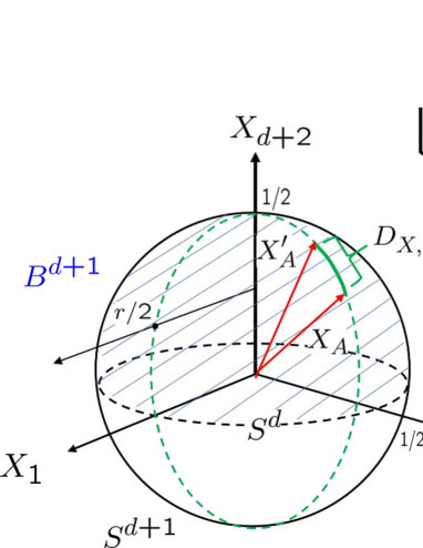
Figure 20: Bures geometry of $S=1/2$ is equal to the hyper-hemisphere

7 Summary

Leveraging the analogies to the Landau models, we explored a higher dimensional formulation of the Zeeman-Dirac models and the Bloch hyper-sphere. The $SO(3)$ Zeeman-Dirac model has $2S+1$ eigenvalues ranging from $-S$ to $+S$ with interval $1$. Though a concrete matrix realization, we showed that the $SO(5)$ Zeeman-Dirac model has the same spectrum of the $SO(3)$ model and each level accommodates the $SO(4)$ degeneracy. The $SO(4)$ Zeeman-Dirac model was similarly analyzed to have $2S+1$ energy levels, each of which accommodates the degeneracy attributed to the $SO(3)$ symmetry. These properties are naturally generalized in higher dimensions:

• The $SO(2k+1)$ spin model is defined for any non-negative integer $2S$. The $SO(2k+1)$ Zeeman-Dirac Hamiltonian has the spectrum ranging from $-S$ to $+S$ with interval $1$. There are $2S+1$ energy levels with $SO(2k)$ degeneracies. The distribution of the degeneracies has a peak at the equator of the Bloch $2k$-sphere. This peak becomes sharper, as dimension increases.

• The $SO(2k)$ Zeeman-Dirac model is defined only for odd non-negative integer $2S$. The $SO(2k)$ Zeeman-Dirac Hamiltonian exhibits the spectrum ranging from $-\frac{S}{2}-\frac{1}{4}$ to $+\frac{S}{2}+\frac{1}{4}$ with interval $1/2$ excluding the zero energy level. There are $2S+1$ energy levels with $SO(2k-1)$ degeneracies. The distribution of the degeneracies has two peaks on the opposite latitudes of both two hemispheres of the Bloch $2k-1$-sphere. These two peaks approach the equator, as dimension increases.

The $d$ dimensional Bloch hyper-sphere geometry exists behind the $SO(d+1)$ Zeeman-Dirac model and accounts the particular properties of that model: The $SO(d)$ stabilizer group symmetry of this Bloch hypersphere endows the energy levels with the $SO(2k)$ degeneracies. The $SO(d)$ holonomy group of the Bloch hyper-sphere induces the Wilczek-Zee connection identical to the $SO(d)$ non-Abelian monopole. We investigated the density matrices described by the Bloch hyper-balls and the corresponding von Neumann entropies and Bures metrics. As one moves from the core of Bloch hyper-ball to its hyper-sphere surface, the von Neumann entropy monotonically decreases and reaches its minimum value on the surface. The Bures statistical geometries of these density matrices represent various curved spherical geometries for different dimensions and magnitudes of spin. In particular, they show qualitatively different behaviors depending on the parity of the dimensions. The Bures geometries for $S=1/2$ were explicitly calculated and identified as the hyper-hemispheres with the same dimensions as the Bloch hyper-balls.

It may be worthwhile to mention that the quantum Nambu matrix geometry serves as the underlying geometry of M(atrix) theory, playing a crucial role in understanding quantum space-time in the context of string theory. This line of research offers an intriguing crossing point where the exotic concept of non-commutative geometry meets the advance of quantum information and quantum matter. Additionally, it is highly anticipated that further progress in artificial gauge fields and synthetic dimensions may facilitate access to relevant novel physical phenomena in real experiments.

Appendix A Examples of the generalized gamma matrices

For a better understanding, we preset a concrete matrix realization of the $SO(5)$ generalized gamma matrices for $S=1$ and the $SO(4)$ generalized gamma matrices for $S=3/2$.

A.1 $SO(5)$ $\Gamma_{a}$ for $S=1$

The $SO(5)$ gamma matrices with $S=1$ are given by the following $10\times 10$ matrices,

$$\!\!\!\!\!\!\!\!\!\Gamma_{1}\!=\!\!\left(\begin{array}[]{ccc:cccc:ccc}0&0&0&0&\sqrt{2}i&0&0&0&0&0\\ 0&0&0&i&0&0&i&0&0&0\\ 0&0&0&0&0&\sqrt{2}i&0&0&0&0\\ \hdashline 0&-i&0&0&0&0&0&0&i&0\\ -\sqrt{2}i&0&0&0&0&0&0&0&0&\sqrt{2}i\\ 0&0&-\sqrt{2}i&0&0&0&0&\sqrt{2}i&0&0\\ 0&-i&0&0&0&0&0&0&i&0\\ \hdashline 0&0&0&0&0&-\sqrt{2}i&0&0&0&0\\ 0&0&0&-i&0&0&-i&0&0&0\\ 0&0&0&0&-\sqrt{2}i&0&0&0&0&0\end{array}\right)\!\!,~{}~{}\Gamma_{2}\!=\!\!\left(\begin{array}[]{ccc:cccc:ccc}0&0&0&0&\sqrt{2}&0&0&0&0&0\\ 0&0&0&-1&0&0&1&0&0&0\\ 0&0&0&0&0&-\sqrt{2}&0&0&0&0\\ \hdashline 0&-1&0&0&0&0&0&0&1&0\\ \sqrt{2}&0&0&0&0&0&0&0&0&\sqrt{2}\\ 0&0&-\sqrt{2}&0&0&0&0&-\sqrt{2}&0&0\\ 0&1&0&0&0&0&0&0&-1&0\\ \hdashline 0&0&0&0&0&-\sqrt{2}&0&0&0&0\\ 0&0&0&1&0&0&-1&0&0&0\\ 0&0&0&0&\sqrt{2}&0&0&0&0&0\end{array}\right)\!\!,$$ (269)

$$\!\!\!\Gamma_{3}=\left(\begin{array}[]{ccc:cccc:ccc}0&0&0&\sqrt{2}i&0&0&0&0&0&0\\ 0&0&0&0&-i&i&0&0&0&0\\ 0&0&0&0&0&0&-\sqrt{2}i&0&0&0\\ \hdashline-\sqrt{2}i&0&0&0&0&0&0&\sqrt{2}i&0&0\\ 0&i&0&0&0&0&0&0&i&0\\ 0&-i&0&0&0&0&0&0&-i&0\\ 0&0&\sqrt{2}i&0&0&0&0&0&0&-\sqrt{2}i\\ \hdashline 0&0&0&-\sqrt{2}i&0&0&0&0&0&0\\ 0&0&0&0&-i&i&0&0&0&0\\ 0&0&0&0&0&0&\sqrt{2}i&0&0&0\end{array}\right)\!\!,~{}~{}\Gamma_{4}=\left(\begin{array}[]{ccc:cccc:ccc}0&0&0&\sqrt{2}&0&0&0&0&0&0\\ 0&0&0&0&1&1&0&0&0&0\\ 0&0&0&0&0&0&\sqrt{2}&0&0&0\\ \hdashline\sqrt{2}&0&0&0&0&0&0&\sqrt{2}&0&0\\ 0&1&0&0&0&0&0&0&1&0\\ 0&1&0&0&0&0&0&0&1&0\\ 0&0&\sqrt{2}&0&0&0&0&0&0&\sqrt{2}\\ \hdashline 0&0&0&\sqrt{2}&0&0&0&0&0&0\\ 0&0&0&0&1&1&0&0&0&0\\ 0&0&0&0&0&0&\sqrt{2}&0&0&0\end{array}\right),$$ (290)

$$\Gamma_{5}=\left(\begin{array}[]{ccc:cccc:ccc}2&0&0&0&0&0&0&0&0&0\\ 0&2&0&0&0&0&0&0&0&0\\ 0&0&2&0&0&0&0&0&0&0\\ \hdashline 0&0&0&0&0&0&0&0&0&0\\ 0&0&0&0&0&0&0&0&0&0\\ 0&0&0&0&0&0&0&0&0&0\\ 0&0&0&0&0&0&0&0&0&0\\ \hdashline 0&0&0&0&0&0&0&-2&0&0\\ 0&0&0&0&0&0&0&0&-2&0\\ 0&0&0&0&0&0&0&0&0&-2\end{array}\right),$$ (301)

which satisfy

$$\sum_{a=1}^{5}\Gamma_{a}\Gamma_{a}=12\cdot\boldsymbol{1}_{10}.$$ (302)

The corresponding $SO(5)$ generators, $\Sigma_{ab}=-i\frac{1}{4}[\Gamma_{a},\Gamma_{b}]$, satisfy $\sum_{a<b=1}^{5}{\Sigma_{ab}}\Sigma_{ab}=6\cdot\boldsymbol{1}_{6}$. The $SO(4)$ decomposition

$$(p,q)=(2,0)~{}~{}\rightarrow~{}~{}(s_{L},s_{R})=(1,0)\oplus(1/2,1/2)\oplus(0,1)$$ (303)

implies that the $SO(4)$ matrices of $\Sigma_{ab}$ take the following form

$$\Sigma_{\mu\nu}=\begin{pmatrix}\Sigma_{\mu\nu}^{(1,0)}&0&0\\ 0&\Sigma_{\mu\nu}^{(1/2,1/2)}&0\\ 0&0&\Sigma_{\mu\nu}^{(0,1)}\end{pmatrix},$$ (304)

where

$$\Sigma_{\mu\nu}^{(1,0)}=\eta_{\mu\nu}^{i}S_{i}^{(1)},~{}~{}~{}~{}\Sigma_{\mu\nu}^{(1/2,1/2)}=\frac{1}{2}\eta_{\mu\nu}^{(+)i}\sigma_{i}\otimes\boldsymbol{1}_{2}+\boldsymbol{1}_{2}\otimes\frac{1}{2}{\eta}_{\mu\nu}^{(-)i}\sigma_{i},~{}~{}~{}~{}\Sigma_{\mu\nu}^{(0,1)}={\eta}_{\mu\nu}^{(-)i}S_{i}^{(1)}.$$ (305)

We can confirm (304) using (301) explicitly.

A.2 $SO(4)$ $\mathit{\Gamma}_{\mu}$ for $S=3/2$

The $SO(5)$ gamma matrices with $S=3/2$ are given by 20$\times$20 matrices. According to the $SO(4)$ subgroup decomposition

$$(p,q)=(3,0)~{}~{}\longrightarrow~{}~{}(s_{L},s_{R})=(3/2,0)\oplus(1,1/2)\oplus(1/2,1)\oplus(0,3/2)$$ (306)

or

$$\boldsymbol{20}~{}~{}\longrightarrow~{}~{}\boldsymbol{4}\oplus\boldsymbol{6}\oplus\boldsymbol{6}\oplus\boldsymbol{4},$$ (307)

the $SO(4)$ subspace of our interest $(1,1/2)\bigoplus(1/2,1)$ corresponds to $\boldsymbol{6}\oplus\boldsymbol{6}$ in (307). Therefore, the $SO(4)$ gamma matrices with $S=3/2$ are given by the following $12\times 12$ matrices:

$$\mathit{\Gamma}_{\mu}=\begin{pmatrix}0&Y_{\mu}\\ {Y_{\mu}}^{\dagger}&0\end{pmatrix},~{}~{}~{}~{}~{}\mathit{\Gamma}_{5}=\begin{pmatrix}\boldsymbol{1}_{6}&0\\ 0&-\boldsymbol{1}_{6}\end{pmatrix},$$ (308)

where

$$Y_{1}\equiv\begin{pmatrix}0&\sqrt{2}i&0&0&0&0\\ 0&0&2i&0&0&0\\ \sqrt{2}i&0&0&0&i&0\\ 0&i&0&0&0&\sqrt{2}i\\ 0&0&0&2i&0&0\\ 0&0&0&0&\sqrt{2}i&0\end{pmatrix},~{}~{}Y_{2}\equiv\begin{pmatrix}0&\sqrt{2}&0&0&0&0\\ 0&0&2&0&0&0\\ -\sqrt{2}&0&0&0&1&0\\ 0&-1&0&0&0&\sqrt{2}\\ 0&0&0&-2&0&0\\ 0&0&0&0&-\sqrt{2}&0\end{pmatrix},$$

$$Y_{3}\equiv\begin{pmatrix}{2}i&0&0&0&0&0\\ 0&\sqrt{2}i&0&0&0&0\\ 0&-i&0&\sqrt{2}i&0&0\\ 0&0&-\sqrt{2}i&0&i&0\\ 0&0&0&0&-\sqrt{2}i&0\\ 0&0&0&0&0&-2i\end{pmatrix},~{}~{}~{}Y_{3}\equiv\begin{pmatrix}{2}&0&0&0&0&0\\ 0&\sqrt{2}&0&0&0&0\\ 0&1&0&\sqrt{2}&0&0\\ 0&0&\sqrt{2}&0&1&0\\ 0&0&0&0&\sqrt{2}&0\\ 0&0&0&0&0&2\end{pmatrix}.$$ (309)

Matrices (308) satisfy

$$\sum_{\mu=1}^{4}\mathit{\Gamma}_{\mu}\mathit{\Gamma}_{\mu}=12\cdot\boldsymbol{1}_{12}.$$ (310)

We can diagonalize $\mathit{\Gamma}_{4}$ as

$$\mathcal{V}^{\dagger}\mathit{\Gamma}_{4}\mathcal{V}=\begin{pmatrix}2\cdot\boldsymbol{1}_{4}&0&0&0\\ 0&1\cdot\boldsymbol{1}_{2}&0&0\\ 0&0&-1\cdot\boldsymbol{1}_{2}&0\\ 0&0&0&-2\cdot\boldsymbol{1}_{4}\end{pmatrix},$$ (311)

where

$$\mathcal{V}=\frac{1}{\sqrt{6}}\left(\begin{array}[]{cccccc:cccccc}\sqrt{3}&0&0&0&0&0&0&0&-\sqrt{3}&0&0&0\\ 0&1&0&0&-\sqrt{2}&0&\sqrt{2}&0&0&-1&0&0\\ 0&\sqrt{2}&0&0&1&0&-1&0&0&-\sqrt{2}&0&0\\ 0&0&\sqrt{2}&0&0&-1&0&1&0&0&-\sqrt{2}&0\\ 0&0&1&0&0&\sqrt{2}&0&-\sqrt{2}&0&0&-1&0\\ 0&0&0&\sqrt{3}&0&0&0&0&0&0&0&-\sqrt{3}\\ \hdashline\sqrt{3}&0&0&0&0&0&0&0&\sqrt{3}&0&0&0\\ 0&\sqrt{2}&0&0&-1&0&-1&0&0&\sqrt{2}&0&0\\ 0&0&1&0&0&-\sqrt{2}&0&-\sqrt{2}&0&0&1&0\\ 0&1&0&0&\sqrt{2}&0&\sqrt{2}&0&0&1&0&0\\ 0&0&\sqrt{2}&0&0&1&0&1&0&0&\sqrt{2}&0\\ 0&0&0&\sqrt{3}&0&0&0&0&0&0&0&\sqrt{3}\end{array}\right).$$ (312)

The $SO(4)$ matrix generators, $\mathit{\Sigma}_{\mu\nu}$, are represented as

$$\mathit{\Sigma}_{\mu\nu}=\begin{pmatrix}\Sigma_{\mu\nu}^{(1,\frac{1}{2})}&0\\ 0&\Sigma_{\mu\nu}^{(\frac{1}{2},1)}\end{pmatrix}=\begin{pmatrix}\eta_{\mu\nu}^{(+)i}S_{i}^{(1)}\otimes\boldsymbol{1}_{2}+\boldsymbol{1}_{3}\otimes{\eta}_{\mu\nu}^{(-)i}\frac{1}{2}\sigma_{i}&0\\ 0&\eta_{\mu\nu}^{i}\frac{1}{2}\sigma_{i}\otimes\boldsymbol{1}_{3}+\boldsymbol{1}_{2}\otimes{\eta}^{(-)i}_{\mu\nu}S_{i}^{(1)}\end{pmatrix}.$$ (313)

Note that $\mathit{\Sigma}_{\mu\nu}\neq-i\frac{1}{4}[\mathit{\Gamma}_{\mu},\mathit{\Gamma}_{\nu}]$.

Appendix B Matrix-valued quantum geometric tensor

Here, we consider $N$-fold degenerate quantum states represented by a $M\times N$ rectangular matrix $\Psi$. We assume that $\Psi$ satisfies the normalization condition,

$$\Psi^{\dagger}\Psi=\boldsymbol{1}_{N}.$$ (314)

In terms of the rectangular matrix $\Psi$, the quantum geometric tensor [72] may be generalized as a matrix-valued quantity

$$\chi_{\mu\nu}=\partial_{\mu}\Psi^{\dagger}~{}\partial_{\nu}\Psi-\partial_{\mu}\Psi^{\dagger}\Psi\cdot\Psi^{\dagger}\partial_{\nu}\Psi,$$ (315)

which satisfies

$${\chi_{\mu\nu}}^{\dagger}=\chi_{\nu\mu}.$$ (316)

It is straightforward to show that the matrix quantum geometric tensor (315) is covariant under the gauge transformation:

$$\Psi~{}~{}\rightarrow~{}~{}\Psi\cdot g~{}~{}~{}(g^{\dagger}g=\boldsymbol{1}_{N}),~{}~{}~{}~{}\chi_{\mu\nu}~{}~{}\rightarrow~{}~{}g^{\dagger}\chi_{\mu\nu}g.$$ (317)

Reference [95] discusses a field theoretical model of rectangular matrix-valued field with gauge symmetry. The target space of this model is the Grassmannian manifold, $Gr(M,N)\simeq U(M)/(U(N)\otimes U(M-N))$, which naturally realizes a matrix extension of the $\mathbb{C}P^{N-1}=Gr(N,1)$ with the Fubini-Study metric. We adopt the same procedure to explore the matrix version of the quantum geometric tensor. We introduce an auxiliary gauge field and the covariant derivative as

$$A_{\mu}=-i\Psi^{\dagger}\partial_{\mu}\Psi=A_{\mu}^{\dagger},~{}~{}~{}~{}D_{\mu}\Psi\equiv\partial_{\mu}\Psi-i\Psi A_{\mu},~{}~{}~{}(D_{\mu}\Psi)^{\dagger}=\partial_{\mu}\Psi^{\dagger}+iA_{\mu}\Psi^{\dagger},$$ (318)

which transform as

$$A_{\mu}~{}~{}\rightarrow~{}~{}g^{\dagger}A_{\mu}g-ig^{\dagger}\partial_{\mu}g,~{}~{}~{}D_{\mu}\Psi~{}~{}\rightarrow~{}~{}(D_{\mu}\Psi)\cdot g,~{}~{}~{}~{}(D_{\mu}\Psi)^{\dagger}~{}~{}\rightarrow~{}~{}g^{\dagger}\cdot(D_{\mu}\Psi)^{\dagger}.$$ (319)

Matrix $\chi_{\mu\nu}$ is simply represented as

$$\chi_{\mu\nu}=(D_{\mu}\Psi)^{\dagger}~{}D_{\nu}\Psi.$$ (320)

Equation (320) manifestly shows that $\chi_{\mu\nu}$ is not generally gauge invariant, but rather covariant under the transformation (317). Here, we decompose the matrix-valued quantum geometric tensor into its symmetric (Hermitian) part and its antisymmetric (anti-Hermitian) part:

$$\chi_{\mu\nu}=G_{\mu\nu}+i\frac{1}{2}F_{\mu\nu},$$ (321)

where

$$G_{\mu\nu}\equiv\frac{1}{2}(\chi_{\mu\nu}+\chi_{\nu\mu})=\frac{1}{2}((D_{\mu}\Psi)^{\dagger}~{}D_{\nu}\Psi+(D_{\nu}\Psi)^{\dagger}~{}D_{\mu}\Psi),$$ (322a)

$$F_{\mu\nu}\equiv-i(\chi_{\mu\nu}-\chi_{\nu\mu})=-i((D_{\mu}\Psi)^{\dagger}~{}D_{\nu}\Psi-(D_{\nu}\Psi)^{\dagger}~{}D_{\mu}\Psi).$$ (322b)

Equation (316) implies that both $G_{\mu\nu}$ and $F_{\mu\nu}$ are Hermitian:

$${G_{\mu\nu}}^{\dagger}=G_{\mu\nu},~{}~{}~{}{F_{\mu\nu}}^{\dagger}=F_{\mu\nu}.$$ (323)

It is obvious that both $G_{\mu\nu}$ and $F_{\mu\nu}$ covariantly transform as

$$G_{\mu\nu}~{}~{}\rightarrow~{}~{}g^{\dagger}G_{\mu\nu}g,~{}~{}~{}~{}~{}~{}F_{\mu\nu}~{}~{}\rightarrow~{}~{}g^{\dagger}F_{\mu\nu}g.$$ (324)

Using $A_{\mu}$, we can represent $G_{\mu\nu}$ and $F_{\mu\nu}$ as

$$G_{\mu\nu}=\frac{1}{2}(\partial_{\mu}\Psi^{\dagger}\partial_{\nu}\Psi+\partial_{\nu}\Psi^{\dagger}\partial_{\mu}\Psi)-\frac{1}{2}(A_{\mu}A_{\nu}+A_{\nu}A_{\mu}),$$ (325a)

$$F_{\mu\nu}=\partial_{\mu}A_{\nu}-\partial_{\nu}A_{\mu}+i[A_{\mu},A_{\nu}].$$ (325b)

Note that $F_{\mu\nu}$ (325b) stand for the field strength of the gauge field $A_{\mu}$, while $G_{\mu\nu}$ (325a) cannot be solely expressed in terms of $A_{\mu}$. Matrix $G_{\mu\nu}$ may be considered as a matrix-valued quantum metric, because its trace signifies the quantum metric,

$$g_{\mu\nu}\equiv\text{tr}(G_{\mu\nu}).$$ (327)

When considering a group with traceless generators, such as a special unitary group or a special orthogonal group (except for $SO(2)$), the trace of the quantum geometric tensor directly yields the quantum metric,

$$\text{tr}(\chi_{\mu\nu})=\text{tr}(G_{\mu\nu})+i\frac{1}{2}\overbrace{\text{tr}(F_{\mu\nu})}^{=0}=g_{\mu\nu}~{}~{}\text{for}~{}~{}SU(N),~{}SO(N\geq 3),~{}\text{etc}.$$ (328)

Appendix C $SO(4)$ monopole harmonics from the $SO(4)$ non-linear realization

We revisit the analysis of the $SO(4)$ Landau model [55, 78] from the perspective of non-linear realization.

C.1 $SO(3)$ decomposition of the $SO(4)$ irreducible representation

Due to $SO(4)\simeq SU(2)_{L}\otimes SU(2)_{R}$, the $SO(4)$ irreducible representation is indexed by $SU(2)$ bi-spins, $s_{L}$ and $s_{R}$. The $SO(4)$ matrix generators of irreducible representation are generally given by

$$\Sigma_{\mu\nu}^{(s_{L},s_{R})}=\eta^{(+)i}_{\mu\nu}S_{i}^{(s_{L})}\otimes\boldsymbol{1}_{2s_{R}+1}+{\eta}^{(-)i}_{\mu\nu}\boldsymbol{1}_{2s_{L}+1}\otimes S_{i}^{(s_{R})},$$ (329)

where $\eta_{\mu\nu}^{(\pm)i}$ are the ‘t Hoof tensors (59) and $S_{i}^{(s_{L})}$ and $S_{i}^{(s_{R})}$ signify the $SU(2)$ matrices of the spins $s_{L}$ and $s_{R}$, respectively $(\sum_{i=1}^{3}{S_{i}^{(s_{L/R})}}S_{i}^{(s_{L/R})}=s_{L/R}(s_{L/R}+1)\boldsymbol{1}_{2s_{L/R}+1})$. In detail,

$$\Sigma_{ij}^{(s_{L},s_{R})}=\epsilon_{ijk}(S_{k}^{(s_{L})}\otimes\boldsymbol{1}_{2s_{R}+1}+\boldsymbol{1}_{2s_{L}+1}\otimes S_{k}^{(s_{R})}),$$ (330a)

$$\Sigma_{i4}^{(s_{L},s_{R})}=-\Sigma_{4i}^{(s_{L},s_{R})}=S_{i}^{(s_{L})}\otimes\boldsymbol{1}_{2s_{R}+1}-\boldsymbol{1}_{2s_{L}+1}\otimes S_{i}^{(s_{R})}.$$ (330b)

Sum of their squares provides

$$\sum_{\mu>\nu=1}^{4}{\Sigma_{\mu\nu}^{(s_{L},s_{R})}}~{}{\Sigma_{\mu\nu}^{(s_{L},s_{R})}}=2(s_{L}(s_{L}+1)+s_{R}(s_{R}+1))\boldsymbol{1}_{(2s_{L}+1)(2s_{R}+1)}.$$ (331)

Notice that $\Sigma_{ij}^{(s_{L},s_{R})}$ (330a) is the tensor product of two $SU(2)$ spins, which is irreducibly decomposed by the $SU(2)$ group as

$$O~{}\Sigma_{ij}^{(s_{L},s_{R})}~{}O^{t}=\epsilon_{ijk}\bigoplus_{J=|s_{L}-s_{R}|}^{s_{L}+s_{R}}S_{k}^{(J)},$$ (332)

where $O$ denotes an orthogonal matrix made of the Clebsch-Gordan coefficients,

$$O_{\alpha\beta}\equiv C^{(JM)}_{s_{L},m_{L};~{}s_{R},m_{R}},~{}~{}~{}~{}(\alpha,\beta=1,2,\cdots,(2s_{L}+1)(2s_{R}+1))$$ (333)

with identification

$$\alpha\equiv(J,M)~{}~{}~{}~{}~{}~{}~{}~{}~{}(J=s_{L}+s_{R},s_{L}+s_{R}-1,\cdots,|s_{L}-s_{R}|,~{}~{}M=J,J-1,\cdots,-J),$$

$$\beta\equiv(m_{L},m_{R})~{}~{}~{}~{}~{}~{}(m_{L}=s_{L},s_{L}-1,\cdots,-s_{L},~{}~{}~{}m_{R}=s_{R},s_{R}-1,\cdots,-s_{R}).$$ (334)

C.2 $SO(4)$ monopole harmonics

Using the parametrization of $x_{\mu}$ (121), we introduce the non-linear realization matrix

$$\Psi^{(s_{L},s_{R})}\equiv e^{-i\sum_{i=1}^{3}\chi y_{i}\Sigma_{i4}^{(s_{L},s_{R})}}=e^{(-i\chi\sum_{i=1}^{3}y_{i}S_{i}^{(s_{L})})\otimes\boldsymbol{1}_{2s_{R}+1}+\boldsymbol{1}_{2s_{L}+1}\otimes(i\chi\sum_{i=1}^{3}y_{i}S_{i}^{(s_{R})})},$$ (335)

or

$$\Psi^{(s_{L},s_{R})}=D^{(s_{L})}(\boldsymbol{\chi})\otimes D^{(s_{R})}(-\boldsymbol{\chi})$$ (336)

where

$$D^{(s_{L})}(\boldsymbol{\chi})\equiv e^{-i\chi\sum_{i=1}^{3}y_{i}S_{i}^{(s_{L})}},~{}~{}~{}~{}~{}D^{(s_{R})}(-\boldsymbol{\chi})\equiv e^{i\chi\sum_{i=1}^{3}y_{i}S_{i}^{(s_{R})}}.$$ (337)

The covariant derivative is defined as

$$D_{\mu}^{(s_{L},s_{R})}=\partial_{\mu}+iA_{\mu}^{(s_{L},s_{R})}$$ (338)

where

$$A_{\mu}^{(s_{L},s_{R})}dx_{\mu}=-\frac{1}{1+x_{4}}\Sigma_{ij}^{(s_{L},s_{R})}x_{j}dx_{i}=-\frac{1}{1+x_{4}}\epsilon_{ijk}(S_{k}^{(s_{L})}\otimes\boldsymbol{1}_{2s_{R}+1}+\boldsymbol{1}_{2s_{L}+1}\otimes S_{k}^{(s_{R})})x_{j}dx_{i}.$$ (339)

Matrix $\Psi^{(s_{L},s_{R})}$ satisfies

$$L_{\mu\nu}^{(s_{L},s_{R})}\Psi^{(s_{L},s_{R})}=\Psi^{(s_{L},s_{R})}\Sigma_{\mu\nu}^{(s_{L},s_{R})},$$ (340)

where

$$L_{\mu\nu}^{(s_{L},s_{R})}=-ix_{\mu}D_{\nu}^{(s_{L},s_{R})}+ix_{\nu}D_{\mu}^{(s_{L},s_{R})}+F_{\mu\nu}^{(s_{L},s_{R})}.$$ (341)

Therefore, with

$$\Psi^{(s_{L},s_{R})}=\begin{pmatrix}\boldsymbol{\Psi}^{(s_{L},s_{R})}_{1}&\boldsymbol{\Psi}^{(s_{L},s_{R})}_{2}&\boldsymbol{\Psi}^{(s_{L},s_{R})}_{3}&\cdots&\boldsymbol{\Psi}^{(s_{L},s_{R})}_{(2s_{L}+1)(2s_{R}+1)}\end{pmatrix},$$ (342)

we demonstrate

$$L_{\mu\nu}^{(s_{L},s_{R})}\boldsymbol{\Psi}^{(s_{L},s_{R})}_{\alpha}=\boldsymbol{\Psi}^{(s_{L},s_{R})}_{\beta}(\Sigma_{\mu\nu}^{(s_{L},s_{R})})_{\beta\alpha}.$$ (343)

From (332), we can represent the $SU(2)$ irreducible decomposition of Eq.(343)

$$OL_{\mu\nu}^{(s_{L},s_{R})}O^{t}\cdot O\boldsymbol{\Psi}^{(s_{L},s_{R})}_{\alpha}=O\boldsymbol{\Psi}^{(s_{L},s_{R})}_{\beta}(\Sigma_{\mu\nu}^{(s_{L},s_{R})})_{\beta\alpha}$$ (344)

as

$$(\bigoplus_{J=|s_{L}-s_{R}|}^{s_{L}+s_{R}}L_{\mu\nu}^{(J)})\boldsymbol{\Phi}^{(s_{L},s_{R})}_{\alpha}=\boldsymbol{\Phi}^{(s_{L},s_{R})}_{\beta}(\Sigma_{\mu\nu}^{(s_{L},s_{R})})_{\beta\alpha},$$ (345)

where

$$\boldsymbol{\Phi}^{(s_{L},s_{R})}_{\alpha}\equiv O\boldsymbol{\Psi}^{(s_{L},s_{R})}_{\alpha},~{}~{}~{}~{}~{}L_{\mu\nu}^{(J)}\equiv-ix_{\mu}D^{(J)}_{\nu}+ix_{\nu}D^{(J)}_{\mu}+F^{(J)}_{\mu\nu},$$ (346)

with

$$A^{(J)}_{\mu}dx_{\mu}\equiv-\frac{1}{1+x_{4}}\epsilon_{ijk}x_{j}S^{(J)}_{k}dx_{i}.$$ (347)

Assume that $J$ includes $S$,

$$J=s_{L}+s_{R},s_{L}+s_{R}-1,\cdots,S,\cdots,|s_{L}-s_{R}|.$$ (348)

We introduce the $(2S+1)$ component “vector” $\boldsymbol{\phi}_{\alpha}^{(s_{L},s_{R})}$ with its $A$th component being

$$(\boldsymbol{\phi}_{\alpha}^{(s_{L},s_{R})})_{A}\equiv C^{S,A}_{s_{L},m_{L};~{}s_{R},m_{R}}(\boldsymbol{\Psi}_{\alpha}^{(s_{L},s_{R})})_{m_{L},m_{R}},~{}~{}~{}~{}~{}~{}(\alpha=1,2,\cdots,(2s_{L}+1)(2s_{R}+1),~{}~{}~{}A=S,S-1,\cdots,-S),$$ (349)

or

$$(\boldsymbol{\phi}_{m_{L},m_{R}}^{(s_{L},s_{R})})_{A}\equiv C^{S,A}_{s_{L},m^{\prime}_{L};~{}s_{R},m^{\prime}_{R}}D^{(s_{L})}(\boldsymbol{\chi})_{m^{\prime}_{L},m_{L}}D^{(s_{R})}(-\boldsymbol{\chi})_{m^{\prime}_{R},m_{R}},~{}~{}~{}~{}~{}(-s_{L}\leq m_{L}\leq s_{L},~{}~{}-s_{R}\leq m_{R}\leq s_{R})$$ (350)

which is consistent with the expression in Refs.[55, 78]. These $SO(4)$ monopole harmonics satisfy

$$L^{(S)}_{\mu\nu}\boldsymbol{\phi}_{m_{L},m_{R}}^{(s_{L},s_{R})}=\boldsymbol{\phi}_{m_{L},m_{R}}^{(s_{L},s_{R})}\Sigma_{\mu\nu}^{(s_{L},s_{R})}$$ (351)

where

$$L_{\mu\nu}^{(S)}=-ix_{\mu}D^{(S)}_{\nu}+ix_{\nu}D^{(S)}_{\mu}+F^{(S)}_{\mu\nu},$$ (352)

with

$$A^{(S)}_{\mu}dx_{\mu}=-\frac{1}{1+x_{4}}\epsilon_{ijk}x_{j}S^{(S)}_{k}dx_{i}.$$ (353)

Consequently,

$$\sum_{\mu>\nu}{L^{(S)}_{\mu\nu}}^{2}~{}\boldsymbol{\phi}_{m_{j},m_{k}}^{(s_{L},s_{R})}=2(s_{L}(s_{L}+1)+s_{R}(s_{R}+1))\boldsymbol{\phi}_{m_{j},m_{k}}^{(s_{L},s_{R})}.$$ (354)

The ortho-normal relations of the $SO(4)$ monopole harmonics are given by

$$\int_{S^{3}}d\Omega_{3}~{}{\boldsymbol{\phi}_{\alpha}^{(s_{L},s_{R})}}^{\dagger}\boldsymbol{\phi}_{\beta}^{(s_{L},s_{R})}=A(S^{3})\frac{D_{SO(3)}(S)}{D_{SO(4)}(s_{L},s_{R})}\delta_{\alpha\beta}=2\pi^{2}\frac{2S+1}{(2s_{L}+1)(2s_{R}+1)}\delta_{\alpha\beta},$$ (355)

where $d\Omega_{3}=\sin^{2}\chi\sin\theta d\chi d\theta d\phi$, $A(S^{3})=\int_{S^{3}}d\Omega_{3}=2\pi^{2}$ and $D_{SO(4)}(s_{L},s_{R})=(2s_{L}+1)(2s_{R}+1)$.

Appendix D Nested Bloch four-spheres from higher Landau levels

Here, we extend the analysis of the $SO(5)$ lowest Landau level of Sec.3.2 to higher Landau levels. As the quantum matrix geometry exhibits a nested structure in higher Landau levels [64, 59], the corresponding Zeeman-Dirac model also exhibits a nested structure. The Landau level $N$ and the spin index $S$ of the $SU(2)$ monopole are identified with the $SO(5)$ Casimir indices as

$$(p,q)=(N+2S,N)$$ (356)

or $[l_{1},l_{2}]=[\frac{1}{2}(p+q),\frac{1}{2}(p-q)]=[N+S,S]$. The degeneracy of the $N$ th Landau level is given by

$$D(N,S)\equiv\frac{1}{6}(N+1)(2S+1)(N+2S+2)(2N+2S+3).$$ (357)

Evaluating the matrix coordinates with the $N$th Landau level eigenstates

$$(\Gamma_{a})_{\alpha\beta}~{}\propto~{}\langle\psi_{\alpha}|x_{a}|\psi_{\beta}\rangle,$$ (358)

we can derive $D(N,S)\times D(N,S)$ generalized gamma matrices $\Gamma_{a=1,2,3,4,5}$ [64], which satisfy

$$\sum_{a=1}^{5}\Gamma_{a}\Gamma_{a}=4\frac{(N+S+2)S(S+1)}{N+S+1}\boldsymbol{1}_{D(N,S)}~{}\propto~{}\boldsymbol{1}.$$ (359)

Diagonal matrix $\Gamma_{5}$ is given by (see Fig.21 also)

$$\Gamma_{5}=\frac{2}{N+S+1}\bigoplus_{n=0}^{N}(n+S+1)~{}\biggl{(}\bigoplus_{\lambda=-S}^{S}\lambda\cdot\boldsymbol{1}_{(n+S+1+\lambda)(n+S+1-\lambda)}\biggr{)}.$$ (360)

With the $SO(5)$ matrix generators $\Sigma_{ab}$ of the representation (356), $\Gamma_{a}$ transform as an $SO(5)$ vector [64]

$$[\Sigma_{ab},\Gamma_{c}]=i\delta_{ac}\Gamma_{b}-i\delta_{bc}\Gamma_{a}.$$ (362)

The $SO(5)$ Zeeman-Dirac Hamiltonian is constructed as

$$H=\sum_{a=1}^{5}x_{a}\cdot\frac{1}{2}\Gamma_{a}.~{}~{}~{}~{}(\sum_{a=1}^{5}x_{a}x_{a}=1)$$ (363)

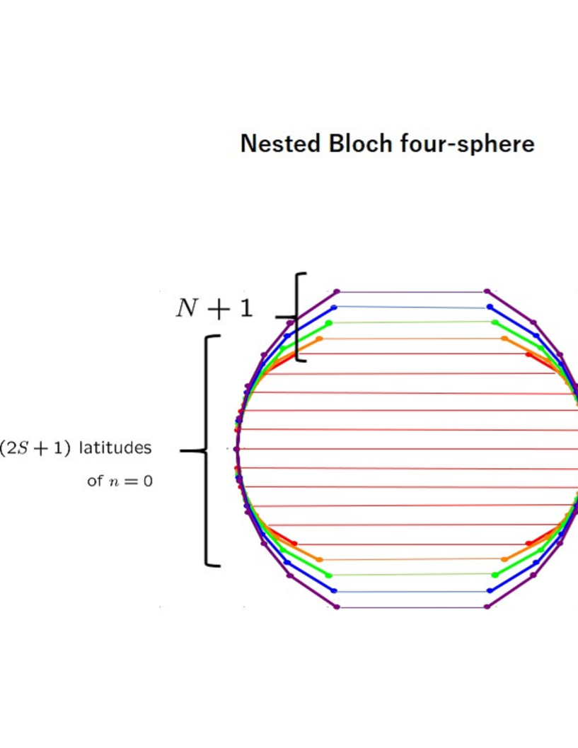
Figure 21: The $SO(5)$ Zeeman-Dirac model for $(p,q)=(2S+N,N)$. Taken from [64].

Since $\Gamma_{a}$ transform as an $SO(5)$ vector (362), $\Psi=e^{i\xi\sum_{\mu=1}^{4}y_{\mu}\Sigma_{\mu 5}}$ diagonalizes the Hamiltonian

$$\Psi^{\dagger}~{}\sum_{a=1}^{5}(x_{a}\cdot\frac{1}{2}\Gamma_{a})~{}\Psi=\frac{1}{2}\Gamma_{5}.$$ (364)

Therefore, the eigenvalues of the Hamiltonian (363) are given by

$$\frac{n+S+1}{N+S+1}\lambda.~{}~{}~{}~{}(n=0,1,2,\cdots,N,~{}~{}~{}\lambda=S,S-1,S-2,\cdots,-S)$$ (365)

Notice that the energy levels are indexed by two quantities, $n$ and $\lambda$, and the degeneracies are given by $(n+S+\lambda+1)(n+S-\lambda+1)$. Consequently, there are $(N+1)(2S+1)$ energy levels (Fig.21). The Wilczek-Zee connection in the energy level (365) is equal to the $SO(4)$ monopole gauge field:

$$A^{(s_{L},s_{R})}=-\frac{1}{1+x_{5}}\Sigma_{\mu\nu}^{(s_{L},s_{R})}x_{\nu}dx_{\mu},$$ (366)

where $\Sigma_{\mu\nu}^{(s_{L},s_{R})}$ are given by (329) with

$$(s_{L},s_{R})\equiv(\frac{n}{2}+\frac{S}{2}+\frac{\lambda}{2},\frac{n}{2}+\frac{S}{2}-\frac{\lambda}{2}).$$ (367)

The correspondence to the Landau model eigenstates is as follows. For the $SO(5)$ Landau model in the $SO(4)$ monopole background with bi-spin index $(I_{+}/2,I_{-}/2)$, the Landau level $L$ and $l$th sector are related to the $SO(5)$ and $SO(4)$ Casimir indices as

$$(p,q)=(L+I_{+}+I_{-}-l,L+l),$$ (368a)

$$(s_{L},s_{R})=(\frac{I_{+}}{2},\frac{I_{-}}{2}).$$ (368b)

For the $SO(5)$ Zeeman-Dirac model, the relations are given by (356) and (367). Consequently, their identification proceeds as follows:

$$L=N-n,~{}l=n,$$ (369a)

$$\frac{I_{+}}{2}=\frac{n}{2}+\frac{S}{2}+\frac{\lambda}{2},~{}~{}~{}~{}~{}\frac{I_{-}}{2}=\frac{n}{2}+\frac{S}{2}-\frac{\lambda}{2}.$$ (369b)

Assume that ${\Psi_{\sigma}}$ denote the degenerate $SO(5)$ spin-coherent states all of which are aligned to the direction of the $\lambda$-latitude on the $n$th shell (see the left of Fig.21) and $\boldsymbol{\psi}^{(n)}_{\alpha,N-n}$ stand for the $(N-n)$th Landau level eigenstates of the $n$-sector in the $SO(4)$ monopole background with the bi-spin index, $(\frac{n}{2}+\frac{S}{2}+\frac{\lambda}{2},\frac{n}{2}+\frac{S}{2}-\frac{\lambda}{2})$. They are related as

$$\begin{pmatrix}\Psi_{1}&\Psi_{2}&\cdots&\Psi_{(n+S+\lambda+1)(n+S-\lambda+1)}\end{pmatrix}=\begin{pmatrix}{\boldsymbol{\psi}^{(n)}_{1,N-n}}^{\dagger}\\ {\boldsymbol{\psi}^{(n)}_{2,N-n}}^{\dagger}\\ {\boldsymbol{\psi}^{(n)}_{3,N-n}}^{\dagger}\\ \vdots\\ {\boldsymbol{\psi}^{(n)}_{D(N,S),N-n}}^{\dagger}\end{pmatrix}.$$ (370)

Appendix E $SO(d+1)$ minimal Zeeman-Dirac model

We investigate the $SO(d+1)$ Zeeman-Dirac models made of the spinor representation gamma matrices.

E.1 $SO(d+1)$ spinor representation matrices

The $SO(2k+1)$ gamma matrices $\gamma_{a=1,2,\cdots,2k+1}$ are given by

$$\gamma_{\mu=1,2,\cdots,2k}=\begin{pmatrix}0&\bar{g}_{\mu}\\ g_{\mu}&0\end{pmatrix},~{}~{}~{}\gamma_{2k+1}=\begin{pmatrix}\boldsymbol{1}_{2^{k-1}}&0\\ 0&-\boldsymbol{1}_{2^{k-1}}\end{pmatrix},$$ (371)

where

$$g_{\mu}\equiv\{-i\gamma^{\prime}_{i},\boldsymbol{1}_{2^{k-1}}\},~{}~{}\bar{g}_{\mu}\equiv\{i\gamma^{\prime}_{i},\boldsymbol{1}_{2^{k-1}}\},$$ (372)

with $SO(2k-1)$ gamma matrices $\gamma^{\prime}_{i=1,2,\cdots,2k-1}$. Matrices (371) satisfy

$$\{\gamma_{a},\gamma_{b}\}=2\delta_{ab}\boldsymbol{1}_{2^{k}},$$ (373)

and their commutators provide the $SO(2k+1)$ matrix generators,

$$\sigma_{ab}\equiv-i\frac{1}{4}[\gamma_{a},\gamma_{b}].$$ (374)

Matrices $\sigma_{\mu\nu}$ are the matrix generators of the $SO(2k)$ group:

$$\sigma_{\mu\nu}=\begin{pmatrix}\sigma_{\mu\nu}^{[+1/2]}&0\\ 0&\sigma_{\mu\nu}^{[-1/2]}\end{pmatrix},$$ (375)

where

$$\sigma_{ij}^{[+1/2]}=\sigma_{ij}^{[-1/2]}\equiv\sigma^{\prime}_{ij}\equiv-i\frac{1}{4}[\gamma^{\prime}_{i},\gamma^{\prime}_{j}],~{}~{}~{}~{}~{}\sigma_{i,{2k}}^{[+1/2]}=-\sigma_{i,2k}^{[-1/2]}\equiv\frac{1}{2}\gamma^{\prime}_{i}.$$ (376)

E.2 $SO(2k+1)$ minimal Zeeman-Dirac model

The spinor representation of the $SO(2k+1)$ is specified by

$$[1/2,1/2,\cdots,1/2]_{SO(2k+1)}.$$ (377)

We construct the $SO(2k+1)$ minimal Zeeman-Dirac Hamiltonian as

$$H=\sum_{a=1}^{2k+1}x_{a}\cdot\frac{1}{2}\gamma_{a}.~{}~{}~{}~{}~{}(\sum_{a=1}^{2k+1}x_{a}x_{a}=1),\\$$ (378)

Using the non-linear realization matrix

$$\Psi=e^{i\theta_{2k}\sum_{\mu=1}^{2k}y_{\mu}\sigma_{\mu,{2k+1}}}=\cos(\frac{\theta_{2k}}{2})~{}\boldsymbol{1}_{2^{k}}+2i\sin(\frac{\theta_{2k}}{2})\sum_{\mu=1}^{2k}y_{\mu}\sigma_{\mu,{2k+1}}$$

$$~{}~{}=\frac{1}{\sqrt{2(1+x_{2k+1})}}\begin{pmatrix}(1+x_{2k+1})\boldsymbol{1}_{2^{k-1}}&\sum_{\mu=1}^{2k}x_{\mu}\bar{g}_{\mu}\\ \sum_{\mu=1}^{2k}x_{\mu}g_{\mu}&(1+x_{2k+1})\boldsymbol{1}_{2^{k-1}}\end{pmatrix}=(\Psi^{(1/2)}~{}~{}\Psi^{(-1/2)}),$$ (379)

we can diagonalize the Hamiltonian (378):

$$\Psi^{\dagger}H\Psi=\frac{1}{2}\gamma_{2k+1}.$$ (380)

The energy levels are $\pm 1/2$ with degeneracy $2^{k-1}$ for each. Equation (380) is invariant under the $SO(2k)$ transformation,

$$\Psi~{}~{}\rightarrow~{}~{}\Psi\cdot e^{i\frac{1}{2}\omega_{\mu\nu}\sigma_{\mu\nu}}.$$ (381)

We can derive the Bloch vector as

$${\Psi^{(\pm 1/2)}}^{\dagger}\gamma_{a}\Psi^{(\pm 1/2)}=\pm x_{a}\boldsymbol{1}_{2^{k-1}}.$$ (382)

The matrix-valued quantum geometric tensor is given by

$$\chi^{(\pm 1/2)}_{\theta_{\mu}\theta_{\nu}}=\partial_{\theta_{\mu}}{\Psi^{(\pm 1/2)}}^{\dagger}\partial_{\theta_{\nu}}{\Psi^{(\pm 1/2)}}-\partial_{\theta_{\mu}}{\Psi^{(\pm 1/2)}}^{\dagger}{\Psi^{(\pm 1/2)}}~{}{\Psi^{(\pm 1/2)}}^{\dagger}\partial_{\theta_{\nu}}{\Psi^{(\pm 1/2)}}.~{}~{}~{}(\theta_{\mu},\theta_{\nu}=\theta_{2k},\theta_{2k-1},\cdots,\theta,\phi)$$ (383)

Trace of (383) provides the metric of the $2k$-sphere:

$$g_{\theta_{\mu}\theta_{\nu}}^{(\pm 1/2)}=\frac{1}{2}\text{tr}(\chi^{(\pm 1/2)}_{\theta_{\mu}\theta_{\nu}}+\chi^{(\pm 1/2)}_{\theta_{\nu}\theta_{\mu}})=2^{k-3}~{}\text{diag}(1,~{}\sin^{2}\theta_{2k},~{}\sin^{2}\theta_{2k}\sin^{2}\theta_{2k-1},~{}\cdots,~{}\prod_{i=3}^{2k}\sin^{2}\theta_{i},~{}\sin^{2}\theta\prod_{i=3}^{2k}\sin^{2}\theta_{i}).$$ (384)

The Wilczek-Zee connections are derived as

$$A^{(\pm 1/2)}=-i{\Psi^{(\pm 1/2)}}^{\dagger}d\Psi^{(\pm 1/2)}=-\frac{1}{1+x_{2k+1}}\sigma_{\mu\nu}^{[\pm 1/2]}x_{\nu}dx_{\mu},$$ (385)

which coincide with the gauge fields of the $SO(2k)$ monopoles for $\text{ch}_{k}^{(\pm 1/2)}=\pm 1$. The corresponding curvature $F_{\theta_{\mu}\theta_{\nu}}=\partial_{\theta_{\mu}}A_{\theta_{\nu}}-\partial_{\theta_{\nu}}A_{\theta_{\mu}}+i[A_{\theta_{\mu}},A_{\theta_{\nu}}]$ represents the antisymmetric part of the matrix-valued quantum geometric tensor:

$$F_{\theta_{\mu}\theta_{\nu}}^{(\pm 1/2)}=-i(\chi^{(\pm 1/2)}_{\theta_{\mu}\theta_{\nu}}-\chi^{(\pm 1/2)}_{\theta_{\nu}\theta_{\mu}})=\frac{1}{2}e^{\mu^{\prime}}_{~{}\theta_{\mu}}\wedge e^{\nu^{\prime}}_{~{}\theta_{\nu}}\sigma_{\mu^{\prime}\nu^{\prime}}^{[\pm 1/2]},$$ (386)

where $e^{\mu^{\prime}}_{~{}\theta_{\mu}}$ denote the vielbein of $S^{2k}$.

E.3 $SO(2k)$ minimal Zeeman-Dirac model

The spinor representation of the $SO(2k)$ is designated by

$$[1/2,1/2,\cdots,\pm 1/2]_{SO(2k)}.$$ (387)

We introduce the $SO(2k)$ minimal Zeeman-Dirac Hamiltonian as

$$H=\sum_{\mu=1}^{2k}x_{\mu}\cdot\frac{1}{2}\gamma_{\mu}~{}~{}~{}~{}~{}(\sum_{\mu=1}^{2k}x_{\mu}x_{\mu}=1),\\$$ (388)

and the non-linear realization matrix as

$${\Psi}=e^{i\theta_{2k-1}\sum_{i=1}^{2k-1}y_{i}{\sigma}_{i,2k}}=\cos(\frac{\theta_{2k-1}}{2})~{}\boldsymbol{1}_{2^{k}}+2i\sin(\frac{\theta_{2k-1}}{2})~{}\sum_{i=1}^{2k-1}y_{i}{\sigma}_{i,2k}=\begin{pmatrix}{U}&0\\ 0&{U}^{\dagger}\end{pmatrix},$$ (389)

where

$${\sigma}_{i,2k}\equiv\begin{pmatrix}\sigma_{i,2k}^{[+1/2]}&0\\ 0&\sigma_{i,2k}^{[-1/2]}\end{pmatrix}=\frac{1}{2}\begin{pmatrix}\gamma^{\prime}_{i}&0\\ 0&-\gamma^{\prime}_{i}\end{pmatrix},$$ (390a)

$${U}=e^{i{\theta_{2k-1}}\sum_{i=1}^{2k-1}y_{i}\sigma_{i,2k}^{[+1/2]}}=\frac{1}{\sqrt{2(1+x_{2k})}}((1+x_{2k})\boldsymbol{1}_{2^{k-1}}+ix_{i}\gamma^{\prime}_{i}).$$ (390b)

The Hamiltonian (388) is diagonalized as

$$\tilde{{\Psi}}^{\dagger}H\tilde{{\Psi}}=\frac{1}{2}\gamma_{2k+1}$$ (391)

where

$$\tilde{{\Psi}}={\Psi}{V}=\frac{1}{\sqrt{2}}\begin{pmatrix}{U}&-{U}\\ {U}^{\dagger}&{U}^{\dagger}\end{pmatrix}=(\tilde{{\Psi}}^{(1/2)}~{}\tilde{{\Psi}}^{(-1/2)})$$ (392)

with

$${V}=\frac{1}{\sqrt{2}}\begin{pmatrix}\boldsymbol{1}_{2^{k-1}}&-\boldsymbol{1}_{2^{k-1}}\\ \boldsymbol{1}_{2^{k-1}}&\boldsymbol{1}_{2^{k-1}}\end{pmatrix}.$$ (393)

The energy levels are $\pm 1/2$ with degeneracy $2^{k-1}$ for each. Equation (391) is invariant under the $SO(2k-1)$ transformation,

$$\tilde{{\Psi}}~{}~{}\rightarrow~{}~{}\tilde{{\Psi}}\cdot e^{i\frac{1}{2}\omega_{ij}\tilde{\sigma}_{ij}}.~{}~{}~{}~{}~{}~{}(\tilde{\sigma}_{ij}\equiv\mathcal{V}^{\dagger}{\sigma}_{ij}\mathcal{V})$$ (394)

We can derive the Bloch vector as

$$(\tilde{{\Psi}}^{(\pm 1/2)})^{\dagger}\gamma_{\mu}\tilde{{\Psi}}^{(\pm 1/2)}=\pm x_{\mu}\boldsymbol{1}_{2^{k-1}}.$$ (395)

The matrix-valued quantum geometric tensor is given by

$$\chi^{(\pm 1/2)}_{\theta_{i}\theta_{j}}=\partial_{\theta_{i}}(\tilde{{\Psi}}^{(\pm 1/2)})^{\dagger}\partial_{\theta_{j}}{\tilde{{\Psi}}}^{(\pm 1/2)}-\partial_{\theta_{i}}(\tilde{{\Psi}}^{(\pm 1/2)})^{\dagger}{\tilde{{\Psi}}}^{(\pm 1/2)}~{}(\tilde{{\Psi}}^{(\pm 1/2)})^{\dagger}\partial_{\theta_{j}}\tilde{{\Psi}}^{(\pm 1/2)}.~{}~{}~{}(\theta_{i}=\theta_{2k-1},\cdots,\theta_{3},\theta,\phi)$$ (396)

Its symmetric part of $\chi^{(\lambda)}_{\theta_{i}\theta_{j}}$ provides the metric of $(2k-1)$-sphere:

$$g^{(\pm 1/2)}_{\theta_{i}\theta_{j}}=\frac{1}{2}\text{tr}(\chi^{(\pm 1/2)}_{\theta_{i}\theta_{j}}+\chi^{(\pm 1/2)}_{\theta_{j}\theta_{i}})=2^{k-3}~{}\text{diag}(1,~{}\sin^{2}\theta_{2k-1},~{}\sin^{2}\theta_{2k-1}\sin^{2}\theta_{2k-2},~{}\cdots,~{}\prod_{i=3}^{2k-1}\sin^{2}\theta_{i},~{}\sin^{2}\theta\prod_{i=3}^{2k-1}\sin^{2}\theta_{i}).$$ (397)

The Wilczek-Zee connections are derived as

$$-i\tilde{{\Psi}}^{\dagger}d\tilde{{\Psi}}={{V}}^{\dagger}(-i\Psi^{\dagger}d\Psi){{V}}=\begin{pmatrix}{A}^{(+1/2)}&*\\ *&{A}^{(-1/2)}\end{pmatrix},$$ (398)

where $A^{(+1/2)}=A^{(-1/2)}$ is equal to the gauge field of the $SO(2k-1)$ monopole:

$${A}^{(+1/2)} =-i(\tilde{{\Psi}}^{(1/2)})^{\dagger}d\tilde{{\Psi}}^{(1/2)}=-i\frac{1}{2}({U}^{\dagger}d{U}+{U}d{U}^{\dagger})=-\frac{1}{1+x_{2k}}\sigma^{\prime}_{ij}x_{j}dx_{i}$$

$$=-i(\tilde{{\Psi}}^{(-1/2)})^{\dagger}d\tilde{{\Psi}}^{(-1/2)}={A}^{(-1/2)}.$$ (399)

The corresponding curvature $F_{\theta_{i}\theta_{j}}=\partial_{\theta_{i}}A_{\theta_{j}}-\partial_{\theta_{j}}A_{\theta_{i}}+i[A_{\theta_{i}},A_{\theta_{j}}]$ represents the antisymmetric part of (396):

$$F_{\theta_{i}\theta_{j}}^{(1/2)}=-i(\chi^{(1/2)}_{\theta_{i}\theta_{j}}-\chi^{(1/2)}_{\theta_{j}\theta_{i}})=\frac{1}{2}e^{i^{\prime}}_{~{}\theta_{i}}\wedge e^{j^{\prime}}_{~{}\theta_{j}}\sigma^{\prime}_{i^{\prime}j^{\prime}}=F_{\theta_{i}\theta_{j}}^{(-1/2)},$$ (400)

with $e^{i^{\prime}}_{~{}\theta_{i}}$ being the vielbein of $S^{2k-1}$.

References

- [1] Ingemar Bengtsson, Karol Zyczkowski, “Geometry of Quantum States”, Cambridge University Press (2006).
- [2] Michael A. Nielsen, Issac L. Chuang, “Quantum Computation and Quantum Information”, Cambridge University Press (2005).
- [3] Dariusz Chruściński, Andrzej Jamiolkowski, “Geometric Phases in Classical and Quantum Mechanics”, Birkhäuser (2004).
- [4] Arno Bohm, Ali Mostafazadeh, Hiroyasu Koizumi, Qian Niu, Joseph Zwanziger, “The Geometric Phase in Quantum Systems”, Springer (2003).
- [5] Päivi Törmä, “Essay: Where Can Quantum Geometry Lead Us?”, Phys. Rev. Lett. 131 (2023) 240001; arXiv:2312.11516.
- [6] J. Lambert, E. S. Sorensen, “From Classical to Quantum Information Geometry: A Guide for Physicists”, New J. Phys. 25 (2023) 081201; arXiv:2302.13515.
- [7] Felix Bloch, “Nuclear Induction”, Phys. Rev. 70 (1946) 460.
- [8] M. V. Berry, “Quantum phase factors accompanying adiabatic changes”, Proc. R. Soc. Lond. A 392 (1984) 45-57.
- [9] G. Herzberg, H. C. Longuet-Higgins, “Intersection of potential energy surfaces in polyatomic molecules”, Disc. Faraday Soc. 35 (1963) 77.
- [10] Frank Wilczek, A. Zee, “Appearance of Gauge Structure in Simple Dynamical Systems”, Phys. Rev. Lett. 52 (1984) 2111.
- [11] Shaojie Ma, Hongwei Jia, Yangang Bi, Shangqiang Ning, Fuxin Guan, Hongchao Liu, Chenjie Wang, Shuang Zhang, “Gauge Field Induced Chiral Zero Mode in Five-Dimensional Yang Monopole Metamaterials”, Phys.Rev.Lett. 130 (2023) 243801; arXiv:2305.13566.
- [12] Xingen Zheng, Tian Chen, Weixuan Zhang, Houjun Sun, Xiangdong Zhang, “Exploring topological phase transition and Weyl physics in five dimensions with electric circuits”, Phys.Rev.Res. 4 (2022) 033203; arXiv:2209.08492.
- [13] S. Sugawa, F. Salces-Carcoba, A. R. Perry, Y. Yue, I. B. Spielman, “Second Chern number of a quantum-simulated non-Abelian Yang monopole”, Science 360 (2018) 1429-1434.
- [14] Sh. Ma, Y. Bi, Q. Guo, B. Yang, O. You, J. Feng, H.-B. Sun, Sh. Zhang, “Linked Weyl surfaces and Weyl arcs in photonic metamaterials”, Science 373 (2021) 572-576.
- [15] Tracy Li, Lucia Duca, Martin Reitter, Fabian Grusdt, Eugene Demler, Manuel Endres, Monika Schleier-Smith, Immanuel Bloch, Ulrich Schneider, “Bloch state tomography using Wilson lines”, Science 352 (2016) 1094; arXiv:1509.02185.
- [16] Frank Wilczek, “Introduction to quantum matter”, Phys. Scr. B T146 (2012) 014001.
- [17] H.M. Price, O. Zilberberg, T. Ozawa, I. Carusotto, N. Goldman, “Four-Dimensional Quantum Hall Effect with Ultracold Atoms”, Phys. Rev. Lett. 115 (2015) 195303.
- [18] H.M. Price, O. Zilberberg, T. Ozawa, I. Carusotto, N. Goldman, “Measurement of Chern numbers through center-of-mass responses”, Phys. Rev. B 93 (2016) 245113.
- [19] T. Ozawa, H.M. Price,N. Goldman, O. Zilberberg, I. Carusotto, “Synthetic dimensions in integrated photonics: From optical isolation to four-dimensional quantum Hall physics”, Phys. Rev. A 93 (2016) 043827.
- [20] You Wang, Hannah M. Price, Baile Zhang, Y. D. Chong, “Circuit implementation of a four-dimensional topological insulator”, Nature Communications, 11 (2020) 2356; arXiv:2001.07427.
- [21] John R. Klauder, “The action option and a Feynman quantization of spinor fields in terms of ordinary c-numbers”, Ann. Phys. 11 (1960) 123-168.
- [22] J. M. Radcliffe “Some properties of coherent spin states”, J. Phys. A 4 (1971) 313.
- [23] A. M. Perelomov, “Coherent States for Arbitrary Lie Group”, Commun. Math. Phys. 26 (1972) 222-236.
- [24] F. A. Arecchi, Eric Courtens, Robert Gilmore, Harry Thomas, “Atomic coherent states in quantum optics’, Phys. Rev. A 6 (1972) 2211.
- [25] P.A.M. Dirac, “Quantized singularities in the electromagnetic field”, Proc. Royal Soc. London, A133 (1931) 60-72.
- [26] T.T. Wu, C.N. Yang, “Dirac Monopoles without Strings: Monopole Harmonics”, Nucl.Phys. B107 (1976) 365-380.
- [27] F. T. Hioe and J. H. Eberly, “-Level Coherence Vector and Higher Conservation Laws in Quantum Optics and Quantum Mechanics”, Phys. Rev. Lett. 47 (1981) 838.
- [28] Gen Kimura, “The Bloch Vector for N-Level Systems”, Phys. Lett. A 314 (2003) 339; arXiv:quant-ph/0301152.
- [29] Mark S. Byrd, Navin Khaneja, “Characterization of the positivity of the density matrix in terms of the coherence vector representation”, Phys. Rev. A 68 (2003) 062322; arXiv:quant-ph/0302024.
- [30] Ansgar Graf and Frédéric Piéchon, “Berry Curvature and Quantum Metric in -band systems : an Eigenprojector Approach”, Phys. Rev. B 104 (2021) 085114; arXiv:2102.09899.
- [31] Cameron J.D. Kemp, Nigel R. Cooper and F. Nur Ünal, “Nested-sphere description of the N-level Chern number and the generalized Bloch hypersphere”, Phys. Rev. Research 4 (2022) 023120; arXiv:2110.06934.
- [32] J. Anandan, L. Stodolsky, “Some geometrical considerations of Berry’s phase”, Phys. Rev. D 35 (1987) 2597-2600.
- [33] D M Gitman and A L Shelepin, “Coherent states of SU(N) groups”, J. Phys. A: Math. Theor. 26 (1993) 313-327; hep-th/9208017.
- [34] Sven Gnutzmanny and Marek Kuś, “Coherent states and the classical limit on irreducible representations”, J. Phys. A: Math. Gen. 31 (1998) 9871-9896.
- [35] A. V. Gorshkov, M. Hermele, V. Gurarie, C. Xu, P. S. Julienne, J. Ye, P. Zoller, E. Demler, M. D. Lukin, A. M. Rey, “Two-orbital magnetism with ultracold alkaline-earth atoms”, Nature Physics (2010) 289 - 295; arXiv:0905.2610.
- [36] Mark S. Byrd, Luis J. Boya, Mark Mims, E. C. G. Sudarshan, “Geometry of n-state systems, pure and mixed”, Journal of Physics: Conference Series 87 (2007) 012006.
- [37] D. Uskov, A.R.P. Rau, “Geometric phase and Bloch-sphere construction for SU() groups with a complete description of the SU() group”, Phys. Rev. A 78 (2008) 022331; arXiv:0801.2091.
- [38] A. R. P. Rau, “Symmetries and Geometries of Qubits, and Their Uses”, Symmetry 13 (2021) 1732; arXiv:2103.14105.
- [39] C. Alden Mead, “Molecular Kramers Degeneracy and Non-Abelian Adiabatic Phase Factors”, Phys. Rev. Lett. 59 (1987) 161.
- [40] J.E. Avron, L. Sadun, J. Segert, and B. Simon, “Topological Invariants in Fermi Systems with Time-Reversal Invariance”, Phys.Rev.Lett.61 (1988) 1329.
- [41] J.E. Avron, L. Sadun, J. Segert, and B. Simon, “Chern Numbers, Quaternions, and Berry’s Phases in Fermi Systems”, Commun.Math.Phys.124 (1989) 124.
- [42] C. Alden Mead, “The geometric phase in molecular systems”, Rev.Mod.Phys. 64 (1992) 51.
- [43] S.E. Apsel, C.C. Chancey, M.C.M. O’Brien, “Berry phase and the Jahn-Teller system”, Phys.Rev. B 45 (1992) 5251.
- [44] Congjun Wu, Jiang-ping Hu, Shou-cheng Zhang, “Exact SO(5) Symmetry in the Spin-3=2 Fermionic System”, Phys.Rev. Lett. 91 (2003) 186402.
- [45] Jonas Larson, Erik Sjöqvist, Patrik Öhberg, “Conical Intersections in Physics”, Springer (2020).
- [46] Shinsei Ryu, Andreas P. Schnyder, Akira Furusaki, Andreas W. W. Ludwig, “Topological insulators and superconductors: ten-fold way and dimensional hierarchy”, New J. Phys. 12 (2010) 065010; arXiv:0912.2157.
- [47] Péter Lévay, “Geometrical description of SU(2) Berry phases”, Phys. Rev. A 41, 2837 (1990).
- [48] Péter Lévay, “Quaternionic gauge fields and the geometric phase”, J. Math. Phys. 32, 2347 (1991).
- [49] M.T. Johnsson, J.R. Aitchison, “The instanton and the adiabatic evolution of two Kramers doublets”, Jour. Phys. A: Math. Gen. 30 (1997) 2085.
- [50] Chen Ning Yang, “Generalization of Dirac’s monopole to SU2 gauge fields”, J. Math. Phys. 19 (1978) 320.
- [51] Chen Ning Yang, “SU2 monopole harmonics”, J. Math. Phys. 19 (1978) 2622.
- [52] A.A. Belavin, A.M. Polyakov, A.S. Schwartz and Yu. S. Tyupkin, “Pseudoparticle solutions of the Yang-Mills equations”, Phys. Lett. B 59 (1975) 85-87.
- [53] Kazuki Hasebe, “Relativistic Landau Models and Generation of Fuzzy Spheres”, Int.J.Mod.Phys.A 31 (2016) 1650117; arXiv:1511.04681.
- [54] Goro Ishiki, Takaki Matsumoto, Hisayoshi Muraki,, “Kähler structure in the commutative limit of matrix geometry”, JHEP 08 (2016) 042; arXiv:1603.09146.
- [55] Kazuki Hasebe, “ Landau Models and Matrix Geometry”, Nucl.Phys. B 934 (2018) 149-211; arXiv:1712.07767.
- [56] G. Ishiki, T. Matsumoto, H. Muraki, “Information metric, Berry connection, and Berezin-Toeplitz quantization for matrix geometry”, Phys. Rev. D 98 (2018) 026002; arXiv:1804.00900.
- [57] Kaho Matsuura, Asato Tsuchiya, “Matrix geometry for ellipsoids”, Prog. Theor. Exp. Phys. 2020, 033B05.
- [58] V. P. Nair, “Landau-Hall states and Berezin-Toeplitz quantization of matrix algebras”, Phys.Rev. D 102 (2020) 025015; arXiv:2001.05040.
- [59] Kazuki Hasebe, “SO(5) Landau models and nested matrix geometry”, Nucl.Phys. B 956 (2020) 115012; arXiv:2002.05010.
- [60] Hiroyuki Adachi, Goro Ishiki, Takaki Matsumoto, Kaishu Saito, “The matrix regularization for Riemann surfaces with magnetic fluxes”, Phys. Rev. D 101 (2020) 106009; arXiv:2002.02993.
- [61] Kazuki Hasebe, “SO(5) Landau Model and 4D Quantum Hall Effect in The SO(4) Monopole Background”, Phys. Rev. D 105 (2022) 065010; arXiv:2112.03038.
- [62] Harold C. Steinacker, “Quantum (Matrix) Geometry and Quasi-Coherent States”, J. Phys. A: Math. Theor. 54 (2021) 055401; arXiv:2009.03400.
- [63] Hiroyuki Adachi, Goro Ishiki, Satoshi Kanno, “Vector bundles on fuzzy Kähler manifolds”, arXiv:2210.01397.
- [64] Kazuki Hasebe, “Generating Quantum Matrix Geometry from Gauge Quantum Mechanics”, Phys. Rev. D 108 (2023) 126023; arXiv:2310.01051.
- [65] Wei Zhu, Chao Han, Emilie Huffman, Johannes S. Hofmann, and Yin-Chen He, “Uncovering Conformal Symmetry in the 3D Ising Transition: State-Operator Correspondence from a Quantum Fuzzy Sphere Regularization”, Phys.Rev. X 13 (2023) 021009; arXiv:2210.13482.
- [66] Yale Fan, Willy Fischler, and Eric Kubischta, “Quantum error correction in the lowest Landau level”, Phys.Rev. A 107 (2023) 032411; arXiv:2210.16957.
- [67] Gabriel Cuomo, Zohar Komargodski, Márk Mezei, Avia Raviv-Moshe, “Spin Impurities, Wilson Lines and Semiclassics”, JHEP 06 (2022) 112; arXiv:2202.00040.
- [68] Gabriel Cuomo, Anton de la Fuente, Alexander Monin, David Pirtskhalava, Riccardo Rattazzi, “Rotating superfluids and spinning charged operators in conformal field theory”, Phys.Rev. D 97 (2018) 045012; arXiv:1711.02108.
- [69] Gabriel Cuomo, Luca V. Delacretaz, Umang Mehta, “Large Charge Sector of 3d Parity-Violating CFTs”, JHEP 05 (2021) 115; arXiv:
- [70] F.D.M. Haldane, “Fractional quantization of the Hall effect: a hierarchy of incompressible quantum fluid states”, Phys. Rev. Lett. 51 (1983) 605-608.
- [71] J. J. Sakurai, Jim Napolitano, “Modern Quantum Mechanics”, Cambridge University Press (2020).
- [72] J. P. Provost and G. Vallee, “Riemannian Structure on Manifolds of Quantum States”, Commun. Math. Phys. 76 (1980) 289-301.
- [73] Kazuki Hasebe, “A Unified Construction of Skyrme-type Non-linear sigma Models via The Higher Dimensional Landau Models”, Nucl.Phys. B 961 (2020) 115250; arXiv:2006.06152.
- [74] S.C. Zhang and J.P. Hu, “A four dimensional generalization of the quantum Hall effect”, Science 294 (2001) 823; cond-mat/0110572.
- [75] Judith Castelino, Sangmin Lee, Washington Taylor, “Longitudinal 5-branes as 4-spheres in Matrix theory”, Nucl.Phys.B526 (1998) 334-350; hep-th/9712105.
- [76] H. Grosse, C. Klimcik, P. Presnajder, “On Finite 4D Quantum Field Theory in Non-Commutative Geometry”, Commun.Math.Phys. 180 (1996) 429-438; hep-th/9602115.
- [77] Kazuki Hasebe, “Chiral topological insulator on Nambu 3-algebraic geometry”, Nucl.Phys. B 886 (2014) 681-690; arXiv:1403.7816.
- [78] V.P. Nair, S. Randjbar-Daemi, “Quantum Hall effect on , edge states and fuzzy ”, Nucl.Phys. B679 (2004) 447-463; hep-th/0309212.
- [79] Z. Guralnik, S. Ramgoolam, “On the Polarization of Unstable D0-Branes into Non-Commutative Odd Spheres”, JHEP 0102 (2001) 032; hep-th/0101001.
- [80] Sanjaye Ramgoolam, “Higher dimensional geometries related to fuzzy odd-dimensional spheres”, JHEP 0210 (2002) 064; hep-th/0207111.
- [81] Anirban Basu, Jeffrey A. Harvey, “The M2-M5 Brane System and a Generalized Nahm’s Equation”, Nucl.Phys. B713 (2005) 136-150; hep-th/0412310.
- [82] M. M. Sheikh-Jabbari, M. Torabian, “Classification of All 1/2 BPS Solutions of the Tiny Graviton Matrix Theory”, JHEP 0504 (2005) 001; hep-th/0501001.
- [83] K. Hasebe and Y. Kimura, “Dimensional Hierarchy in Quantum Hall Effects on Fuzzy Spheres”, Phys.Lett. B 602 (2004) 255; hep-th/0310274.
- [84] Kazuki Hasebe, “Higher Dimensional Quantum Hall Effect as A-Class Topological Insulator”, Nucl.Phys. B 886 (2014) 952-1002; arXiv:1403.5066.
- [85] Kazuki Hasebe, “Higher (Odd) Dimensional Quantum Hall Effect and Extended Dimensional Hierarchy”, Nucl.Phys. B 920 (2017) 475-520; arXiv:1612.05853.
- [86] See for instance, F. Iachello, “Lie Algebras and Applications”, (Lecture Notes in Physics) Springer (2006).
- [87] Kazuki Hasebe, “Hopf Maps, Lowest Landau Level, and Fuzzy Spheres”, SIGMA 6 (2010) 071; arXiv:1009.1192.
- [88] Joshua DeBellis, Christian Saemann, Richard J. Szabo, “Quantized Nambu-Poisson Manifolds and n-Lie Algebras”, J.Math.Phys.51 (2010) 122303; arXiv:1001.3275.
- [89] Takehiro Azuma, Maxime Bagnoud, “Curved-space classical solutions of a massive supermatrix model”, Nucl.Phys. B 651 (2003) 71-86; hep-th/0209057.
- [90] Takehiro Azuma, “Matrix models and the gravitational interaction”, hep-th/0401120.
- [91] Donald Bures, “An extension of Kakutani’s theorem on infinite product measures to the tensor product of semifinite w*-algebras”, Trans. Am. Math. Soc. 135 (1969) 199.
- [92] Armin Uhlmann, “The Metric of Bures and the Geometric Phase”, in Gielerak et al. (ed.), “Quantum Groups and Related Topics”, Dordrecht: Kluwer Academic Pub.
- [93] Matthias Hübner, “Explicit computation of the Bures distance for density matrices”, Phys. Lett. A 163 (1992) 239.
- [94] See for instance, Chap.8 in Steven Weinberg, “Gravitation and cosmology”, Wiley (1972).
- [95] A.J. MacFarlane, “Generalizations of -models and models, and instantons”, Phys. Lett. B 82 (1979) 239.