Empirical Analysis of Quantum Approximate Optimization Algorithm for Knapsack-based Financial Portfolio Optimization

Abstract

Portfolio optimization is a primary component of the decision-making process in finance, aiming to tactfully allocate assets to achieve optimal returns while considering various constraints. Herein, we proposed a method that uses the knapsack-based portfolio optimization problem and incorporates the quantum computing capabilities of the quantum walk mixer with the quantum approximate optimization algorithm (QAOA) to address the challenges presented by the NP-hard problem. Additionally, we present the sequential procedure of our suggested approach and demonstrate empirical proof to illustrate the effectiveness of the proposed method in finding the optimal asset allocations across various constraints and asset choices. Moreover, we discuss the effectiveness of the QAOA components in relation to our proposed method. Consequently, our study successfully achieves the approximate ratio of the portfolio optimization technique using a circuit layer of $p\geqslant 3$, compared to the classical best-known solution of the knapsack problem. Our proposed methods potentially contribute to the growing field of quantum finance by offering insights into the potential benefits of employing quantum algorithms for complex optimization tasks in financial portfolio management.

1 Introduction

The financial industry plays a remarkable role in the economic health and growth of a country. In the constantly evolving world of financial markets, technological advancements are shaping traditional portfolio optimization methods, presenting new opportunities and challenges; this process involves enlarging assets to reduce risk by offsetting individual risk profiles crucial to the investment process (Speidell et al. 1989). Although there are many portfolio optimization models, they possibly have limitations. For example, the mean–variance model, which provides solutions as percentages of the total budget, can result in fractional allocations of nonfeasible assets (Vaezi et al. 2019). In the constant pursuit of optimization, some studies have explored extensions to portfolio optimization (Loke et al. 2023). Among these, a technique that reformulates portfolio optimization as a knapsack problem has been proposed (Martello and Toth. 1987; Mansini et al. 2015).

In (Vaezi et al. 2019), the knapsack problem was adapted for portfolio optimization by treating all assets included in the portfolio as items. The value or profit of each asset is represented by its expected return, usually estimated using historical data or forecasting techniques. The weight or volume of each item corresponds to a risky asset, typically measured by its standard deviation or the variance–covariance matrix of the assets. The knapsack capacity corresponds to the budget or available capital that can be invested in the portfolio. By reformulating the problem as a knapsack, the primary objective is to maximize the total value or profit of the portfolio while satisfying the capacity constraint and potentially other constraints, such as a target return or a minimum number of assets. However, similar to (Chu and Beasley. 1998), the knapsack problem is considered NP-hard even with polynomial-bounded weights and values. Therefore, exploring new paradigms for optimization owing to computational complexity of solving this problem is crucial (Honggang et al. 2009).

Similarly, the paradigm of quantum computing, leveraging the properties of quantum mechanics, has been developed to solve complex problems intractable for classical computers (Herman et al. 2023). The financial domain is a primary aspect of quantum computing, with applications spanning price derivation, risk modeling, portfolio optimization, and fraud detection (Saxena et al. 2023). As technology redefines problem-solving in finance, the quantum approximate optimization algorithm (QAOA), rooted in quantum computing, offers the promise of efficiently finding approximate solutions for computationally demanding problems within the polynomial-bounded NP optimization complexity class. In (Dam et al. 2021; Kea et al. 2023), the application of QAOA to the knapsack problem is explored for optimization purposes.

Herein, we present an approach that harnesses the efficacy of QAOA in addressing the complex problem of portfolio optimization by reformulating it as a knapsack problem. Although additional research is required, our findings offer valuable insights into the following areas.

• Our proposed model for portfolio selection formulates the problem as a knapsack concern by incorporating the expected return from the Markowitz model and setting the capacity according to the knapsack framework.

• Our study presents a QAOA algorithm using a quantum walk mixer for the knapsack problem while incorporating a shallow circuit layer to decrease computational complexity and improve solution quality.

• Our extensive empirical analysis reveals a consistent enhancement in identifying optimal solutions for the knapsack problem, providing an impressive approximation ratio ranging from 100% to 98%, with 2–5 stock selection cases. We also underscore the potential of quantum algorithms as robust, forward-looking solutions for complex financial optimization.

The paper is organized as follows: Section 2 provides an overview of the relevant background work. Section 3 explores the research concerning the proposed method. Section 4 details our proposed method, including the functionality of each step. Section 5 demonstrates the meticulous design and execution of the experiment to obtain the desired results. Finally, Section 6 dissects the findings of the proposed method, underscoring its achievements and limitations while presenting a comprehensive conclusion, key takeaways, and potential future directions.

2 Background

2.1 Portfolio Optimization

Portfolio optimization is a mathematical framework that maximizes returns while minimizing risks through strategically selecting assets within an investment portfolio (Anagnostopoulos and Mamanis. 2010). This is typically achieved by strategically allocating the proportion of each asset in the portfolio to optimize the risk–return tradeoff by considering the specified risk tolerance. The process involves four steps: i) identifying suitable assets, ii) projecting anticipated yields based on historical data for future forecasts, iii) quantifying the risk by assessing the uncertainty of each asset, and iv) selecting the optimal portfolio that maximizes the expected yield for a given risk level (Gunjan and Bhattacharyya. 2023). One of the various models used in this study was Markowitz model, developed by Harry Markowitz in 1952 (Markowitz. 1976). This analysis is in conjunction with the variance of the rate of return, providing a significant assessment of portfolio risk under a rational framework of assumptions. The Markowitz model represented the maximum expected yield by allocating funds into stocks as follows (Anton Abdulbasah Kamil and Kok. 2006):

$$R_{i}=\sum_{t=1}^{\infty}d_{i}{}_{t}r_{i}{}_{t},$$ (1)

where ${r_{i}}_{t}$ indicates the anticipated return at time $t$ per stock invested in, and ${d_{i}}_{t}$ is the rate at which return in the $i_{th}$ security where time $t$ is discounted back to the presents. The standard deviation—the variance of return—is a statistical measure used as an indicator of the uncertainty or risk linked to return. These statistical indicators effectively measure the extent to which returns deviate unpredictably from the average value over a specific period. The variance represents the degree of variation exhibited by the return $R_{i}$ concerning the expected return $[E(R_{i})]$, as illustrated by the following equation:

$$\sigma_{i}^{2}=\frac{1}{N}\sum_{i=1}^{N}[R_{i}-E(R_{i})]^{2}.$$ (2)

The covariance of returns measures the relative riskiness of a security within a portfolio of securities. For two securities, denoted as $i$ and $j$, the covariance of their returns is defined as

$$\sigma_{i}{}_{j}=E\{[R_{i}-E(R_{i})][R_{j}-E(R)]\}.$$ (3)

Furthermore, covariance can be measured depending on the variability of the two individual return series:

$$\rho_{i}{}_{j}=\frac{\sigma_{i}{}_{j}}{\sigma_{i}\sigma_{j}},$$ (4)

where ${\rho_{i}}_{j}$ is the correlation coefficient of returns, and $\sigma_{i}$ and $\sigma_{j}$ are the standard deviation of $R_{it}$ and $R_{jt}$. As previously stated, an efficient portfolio is characterized by selecting individual assets within the portfolio and weighting each asset. Therefore, the portfolio return is calculated as a weighted average of the returns of the individual investments within the portfolio. Next, $X_{i}$ denoted as the weight and applied to each return of the portfolio takes form as follows:

$$\begin{array}[]{l}R_{p}=\sum_{t=1}^{\infty}\sum_{i=0}^{N}d_{i}{}_{t}r_{i}{}_{t}X_{i}\\ \\ =\sum_{i=0}^{N}X_{i}\left(\sum_{t=1}^{\infty}d_{i}{}_{t}r_{i}{}_{t}\right)\\ \\ =\sum_{i=0}^{N}X_{i}R_{i},\end{array}$$ (5)

where $R_{i}$ is independent of $X_{i}$. The simplified version of the variance of a portfolio can be written as

$$\sigma_{p}^{2}=\sum_{i=0}^{N}X_{i}^{2}\sigma_{i}^{2}+\sum_{i=0}^{N}\sum_{j=1}^{N}X_{i}X_{j}\sigma_{i}{}_{j},$$ (6)

where $\sigma_{p}^{2}$ is the variance of the portfolio, $X_{i}$ is the percentage of the investor’s assets that are allocated to the $i_{th}$ asset, and the $\sigma_{i}^{2}$ represents the variance of the asset $j$ and the covariance between the returns for assets $i$ and $j$ denoted as $\sigma_{i}{}_{j}$. Reportedly, traditional asset allocation methods, such as the Markowitz theorem, provide solutions in percentages, potentially suggesting the allocation of half of a market share, making it impractical (Vaezi et al. 2019). Therefore, proposing a method for determining the number of shares for each asset is crucial; this involves the conversion of expected returns, prices, and budget into interval values and determines the priority and importance of each share by framing it within a knapsack-based model.

2.2 Knapsack Problem

Herein, a given set of items with known sizes is selected and packed into a knapsack with a fixed capacity (Kleywegt and Papastavrou. 1998). This problem is one of the simpler NP-hard problems in combinatorial optimization because it focuses on maximizing an objective function while adhering to a single resource constraint. To find the exact solutions, some techniques have been employed, such as relaxations, bounds, reductions, and other algorithmic approaches (Du and Pardalos. 1998). These techniques include genetic algorithms (Pradhan et al. 2014), dynamic programming (Schäfer et al. 2021), simulated annealing (Delahaye et al. 2019), Tabu search (Lai et al. 2019), and greedy algorithm (Abidin. 2017). These classical approaches are instrumental in providing optimal solutions. Although these conventional approaches are successful and valuable, they are limitations in computation in the classical domain. Furthermore, the new paradigm of quantum computing introduces optimization techniques, including QAOA, to tackle problems such as the knapsack problem, yielding better solutions than classical computation techniques (de la Grand’rive and Hullo. 2019).

2.3 Quantum Approximate Optimization Algorithm (QAOA)

In combinatorial optimization, QAOA excels as solutions tailored for quantum computing while leveraging the strengths of the classical computing (Farhi et al. 2014; Chen et al. 2023). QAOA, a hybrid quantum-classical algorithm, has demonstrated remarkable effectiveness in addressing recent NP-hard problems, including Max-Cut (Crooks. 2018), traveling salesman problem (Zawalska and Rycerz. 2023), and quadratic unconstrained binary optimization (QUBO) (Borle et al. 2021). Given a combonitorial optimization problem involving an N-bit binary string represented as $z=z_{1}\cdot\cdot\cdot z_{N}$, with a classical objective function $f(z):\{0,1\}^{N}\rightarrow\mathbb{R}$ to be maximized (Ausiello et al. 1999). The goal is to find a solution $z$ that satisfies an approximation condition as follows:

$$\begin{array}[]{l}\frac{f(z)}{f_{max}}\geqslant r^{*},\end{array}$$ (7)

where $f_{max}=max_{z}f(z)$, and $r^{*}$ is a desired approximation ratio. Accordingly, the QAOA algorithm tackles this problem by encoding, which involves mapping the classical objective function $f(z)$ into the phase Hamiltonian $H_{c}$ in order to find the optimal eigenvalues:

$$H_{c}|z\rangle=f(z)|z\rangle.$$ (8)

Furthermore, $H_{c}$ operates diagonally on the computational basis states of $2^{N}$ dimensional Hilbert space ($n$-qubit space). Ideally, the performance of the $p$-level QAOA improves with increasing $p$. For the $p$-level QAOA, the state $\ket{+}^{\otimes N}$ is initialized, while the $H_{c}$ and a mixing Hamiltonian:

$$B=\sum_{j=1}^{N}{\sigma_{j}^{x}},$$ (9)

are applied alternately with controlled durations, generating a wave function:

$$\begin{array}[]{l}\ket{\psi_{p}(\vec{\gamma},\vec{\beta})}=e^{-i\beta_{p}B}e^{-i\gamma_{p}Hc}\cdots e^{-i\beta_{1}B}e^{-i\gamma_{1}H_{c}}\ket{+}^{\otimes N}.\end{array}$$ (10)

This variational wave function is parameterized by $2p$ variational parameters, $\gamma$ and $\beta$. The expected value of $H_{c}$ in this variational state is determined through repeated measurements on a computational basis:

$$f_{p}(\vec{\gamma},\vec{\beta})=\bra{\psi_{p}(\vec{\gamma},\vec{\beta})}H_{c}\ket{\psi_{p}(\vec{\gamma},\vec{\beta})}.$$ (11)

Furthermore, a classical computer is used to search for the optimal parameters $(\gamma^{*},\beta^{*})$ and maximize the averaged output $f(\gamma^{*},\beta^{*})$:

$$\left(\overrightarrow{\gamma^{*}},\overrightarrow{\beta^{*}}\ \right)\ =\ arg\ \ \underset{\vec{\gamma},\vec{\beta}}{max}\ f_{p}\ (\vec{\gamma},\vec{\beta}).$$ (12)

Next, the approximate ratio showing the QAOA performance is

$$r\ =\ \frac{f_{p}\ \left(\overrightarrow{\gamma^{*}},\overrightarrow{\beta^{*}}\ \right)}{f_{max}}.$$ (13)

Moreover, searching for the approximate ratio is typically performed by starting a random initial estimate of parameter and performing gradient-based optimization (Zhou et al. 2020).

3 Related Work

Our study builds upon several key pieces of research that delve into the application of QAOA to the knapsack problem concerning portfolio optimization. QAOA has been employed as an optimization method for portfolio optimization. Herein, the portfolio optimization problem is transformed into a binary version. Accordingly, the weight vector is discretized, with the element taking values of either 0 or 1. In (Awasthi et al. 2023), a comprehensive study of quantum computing approaches for multiknapsack problems is proposed by investigating some of the most prominent and state-of-the-art quantum algorithms using different quantum software and hardware tools. Consequently, quantum computing offers the potential for good and fast solutions to multiknapsack optimization problems in various fields, such as logistics (allocating goods to containers), resource allocation in computing (distributing tasks among different servers), and financial portfolio optimization (allocating assets among different investment opportunities).

In  (Brandhofer et al. 2022), the Markowitz models of portfolio optimization were converted into binary knapsacks. A hard constraint model was employed by incorporating hard constraints into the quantum algorithm, involving designing mixing operators based on the constraint conditions. Additionally, a combination of $XY$- and $XYY$-mixers was used to encode the constraints in the quantum circuit. $XY$-mixers were used to mix the quantum state and generate a superposition of feasible solutions, whereas $XYY$-mixers were used to enforce the hard constraints. Moreover, using a hard constraint model ensured that the quantum state evolved between feasible solutions satisfying the constraints while allowing for a high degree of flexibility in opting parameters.

Another intriguing study highlights the strengths of the quantum walk optimization algorithm (QWOA) (Marsh and Wang. 2019) compared to other quantum optimization algorithms while highlighting the challenges posed by the complex and large solution space associated with its lattice structure. Moreover, the quantum mix optimization algorithm (QMOA) was introduced as an extension of QWOA. QMOA enhanced the efficiency of quantum optimization algorithms for portfolio optimization by reducing the number of iterations required for computations (Shunza et al. 2023).

4 Knapsack-based Portfolio Optimization

4.1 Overall Architecture

This section explains how our method processes everything from stock selection to finding the optimal solution. Figure 1 shows that our structured workflow employs a quantum computing approach to portfolio optimization. Initiating with historical stock price data over time, Algorithm 1 calculates the expected returns of the portfolio using the Markowitz portfolio optimization model. These expected returns are crucial in constructing the portfolio as a binary knapsack problem, incorporating computed mean returns, asset weights, and the portfolio’s capacity constraints. This problem is optimized using Algorithm 2, where the approach for optimizing the knapsack-based portfolio optimization problem is employed. At this stage, we prepared the feasible oracle with quantum Fourier transform (QFT) (Weinstein et al. 2001) for conditional checking of the feasibility of our proposed solution to the knapsack problem before constructing QWM, as discussed in (Marsh and Wang. 2019) with QAOA (QWM–QAOA). The result is a bit string revealing which stocks are chosen or omitted from the portfolio. For example, a solution of (1,0) in the portfolio optimization for Stocks A and B means that Stock A is included and Stock B is excluded, thus outlining the final investment strategy.

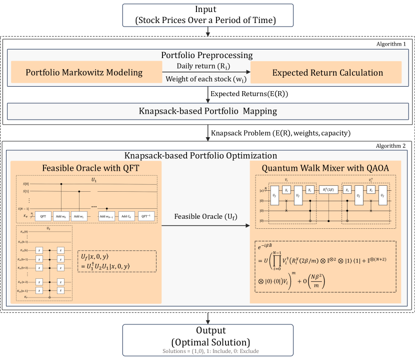
Figure 1: Workflow diagram of the quantum walk mixer with QAOA for knapsack-based portfolio optimization. The process begins with Algorithm 1, where a list of stock prices is collected over time for preparing historical stock prices using the Markowitz model to calculate the expected return. Subsequently, the expected return plays a key role in mapping the knapsack problem, considering the values, weights, and capacity of the portfolio. The optimization process in Algorithm 2 involves employing a quantum walk mixer with QAOA, including the preparation of a feasible oracle before executing the quantum walk mixer with QAOA to enhance the search for the optimal portfolio configuration. Ultimately, the output is a binary string, with $1$ indicating inclusion and $0$ indicating exclusion of stocks from the portfolio, resulting in the optimal solution.

Algorithm 1 Turn portfolio optimization problem into a binary knapsack algorithm

INPUT $start$: start date of stock prices, $end$: end date of stock prices, $stocks$: list of stocks
OUTPUT $problem$: portfolio optimization as a knapsack problem

1:procedure EncodeToKnapsack($start$, $end$, $stocks$)

2:     $prices$ = HistoricalReturn($start$, $end$, $stocks$)

3:     //Calculate the Mean Return

4:     $E(R)$ = ExpectReturn($prices$)

5:     // Set the weights of each stock to 1

6:     for $i\leftarrow 0$ to Length($E(R))$ do

7:         $weights[i]$ = 1

8:     end for

9:     // Define the capacity of the knapsack

10:     $C$ = Length($E(R)$)/2

11:     //Formulate to a knapsack

12:     $problem$ = ($E(R)$, $weights$, $C$)

13:      return $problem$

14:end procedure

Algorithm 1 was initiated by extracting the historical returns of each stock within a specified time frame, ranging from the initiation to the termination dates. This retrieval of historical returns was achieved using the $HistoricalReturn$ function. Subsequently, the algorithm applies the Markowitz model usin the $ExpectReturn$ function, to compute the expected returns denoted as $E(R)$ based on the historical return prices. This variable provides valuable insights into the potential profitability of the selected stocks in the portfolio. In addition, it constructs a covariance matrix serving as an indicator of the correlation in movements between pairs of stocks. From lines $5\textendash 12$, the calculated returns and covariance underwent a transformation to represent the values, weights, and constraints, which are essential components for formulating the knapsack problem. Herein, we set the values to the expected returns ($E(R)$), and the weights for each stock were uniformly set to 1, indicating an equal weight allocation. The algorithm also defined the constraints or capacity for the knapsack problem, with $C$ representing half the length of the expected return array ($Length(E(R))/2$).

Algorithm 2 Optimize knapsack with the QWM-QAOA algorithm

INPUT $problem$: knapsack problem , $p$: layer of circuit, $m$: Trotter step count for QAOA
OUTPUT $ar$: approximation ratio representing optimal choice selection

1:procedure OptimizeKnapsack($problem$, $l$, $m$)

2:     // Determine the number of choices from the problem weights

3:     $choices$ = Length($problem.weights$)

4:     //Calculate the total knapsack weight

5:     $total\_weights$ = TotalWeight($problem.weights$)

6:     // Setup quantum registers for choices and weights

7:     $c_{reg}$ = QuantumRegister($choices$)

8:     $w_{reg}$ = QuantumRegister($total\_weights$)

9:     // Initialize the ancillary quantum register

10:     $a_{reg}$ = QuantumRegister($3$)

11:     // Define quantum mixing and phase operations

12:     $H_{m}$= QWalkMixer($problem$,$m$, $c_{reg}$, $w_{reg}$, $a_{reg}$)

13:     $H_{c}$ = PhaseHamiltonian($c_{reg}$, $problem$)

14:     // Start with a superposition state

15:     $|\psi_{0}\rangle$ = $\ket{+}^{\otimes choices}$

16:     for $k=1$ to $p$ do

17:         if $k\leftarrow 1$  then

18:              $\gamma_{k},\beta_{k}$ = Initialize()

19:         else

20:              ($\gamma_{k}$,$\beta_{k}$) = ($\gamma_{opt},\beta_{opt}$)

21:         end if

22:         // Apply the unitary operators to evolve the state

23:         $U_{B}(\beta_{k})$ = $e^{-i\beta_{k}H_{M}}$

24:         $U_{c}(\gamma_{k})$ = $e^{-i\gamma_{k}H_{c}}$

25:         $\ket{\psi_{k}}=U_{c}(\gamma_{k})U_{B}(\beta_{k})\ket{\psi_{k-1}}$

26:         // Define the QAOA cost function and Optimize it

27:         $cost(\gamma,\beta)$=$\bra{\psi_{k}}H_{c}\ket{\psi_{k}}$

28:         ($\gamma_{opt},\beta_{opt}$)= ShgoOptimizer($cost(\gamma,\beta)$)

29:     end for

30:     // Measure the final state to get probabilities

31:     $probabilities$ = MeasureProbabilities($\ket{\psi_{p}}$

32:     $ar$ = GetOptimalSolution($probabilities$)

33:     return $ar$

34:end procedure

After formulating portfolio optimization into a knapsack problem, we optimized it in Algorithm 2. In this stage, we used QWM–QAOA to prepare the mixing Hamiltonian of QAOA. The steps in lines $2\textendash 10$ involve setting up quantum registers and other preparations necessary for QAOA using a function called $QuantumRegister$. Line $12$ focuses on the preparation of the Mixing Hamiltonian $H_{m}$ using the QWM-QAOA approach; this is realized via the $QwalkMixer$, which requires parameters, such as a predefined trotter step count $m$, the number of quantum registers of choices, weights, and ancillaries. In line 14, we prepare the phase Hamiltonian $H_{c}$, which is a vital component for constructing QAOA, using $PhaseHamiltonian$. The specifications of each method’s construction are presented in Subsection 4.3.

At each circuit layer $p$, the algorithm computed the expectation value (line $28$), facilitating the determination of a new set of optimal $2p$ parameter $(\gamma_{opt},\beta_{opt})$. These optimal parameters were identified using the SHGO method and implemented as $ShgoOptimizer$ in line $29$. Finally, the algorithm measured probabilities (line $31$) through a measurement process. These probabilities were used to determine the optimal solution using the $OptimalChoice$ function to determine the best selection of items represented as $ar$ in line $32$.

4.2 Knapsack-based Portfolio Formulation

Our methodology is based on the fundamental principles of mean–variance optimization, focusing on the Markowitz model. This model historically maximizes the anticipated yield of a portfolio while considering a predetermined level of risk, quantified by the variance of portfolio returns. We denoted the expected return $E(R_{i})$ of stock $i$ by using the mean–variance calculation. Next, we transformed the expected return into a knapsack problem. Subsequently, we extended this model by reinterpreting the expected return as a component of a knapsack problem, thereby aligning portfolio optimization with knapsack problem dynamics; this adaptation involves redefining the expected return of each stock as a value optimized under the constraints of total portfolio risk. This mathematical transformation, which effectively converts portfolio optimization into a knapsack problem, is expressed as follows:

$$\begin{array}[]{l}maximize\;R(x)=\sum_{i=1}^{n}x_{i}E(R_{i})\\ \\ subject\;to\sum_{i=1}^{n}x_{i}\ w_{i}\ \leqslant\ C,\end{array}$$ (14)

where the risk of including stock $i$ in the portfolio, denoted as $w_{i}$, and the total risk tolerance, denoted by $C$, serves as the knapsack capacity. The binary variable $x_{i}$ indicates whether to include stock $i$ in the portfolio, and $E(R_{i})$ represents its expected return values.

4.3 QAOA for the knapsack problem

4.3.1 Feasibility Oracle

The feasibility oracle is used as a hypothetical subroutine that instantly determines whether a proposed solution to the knapsack problem violates any constraints (Chawla et al. 2023). We can explore solutions within a well-defined space of bitstrings by representing our portfolio model as a binary knapsack problem. We defined $K(N)=(0,1)^{N}$ as the set of all possible bitstrings of length $N$ representing potential portfolio choices.

Furthermore, at each possible choice of any of the $N$ items is represented by a bitstring $x\in K(N)$. ). Thus, the subset feasible solution was denoted as $F$ for the knapsack problem, and the feasibility function was defined as

$$f:K(N)\mapsto\{0,1\},x\mapsto f(x)=\begin{cases}1,&\text{if }x\in F\\ 0,&\text{otherwise}.\end{cases}$$ (15)

Considerably, the feasibility oracle to be unitary $U_{f}$ can be described as:

$$\begin{array}[]{l}U_{f}=\ket{x,y}=\ket{x,y\oplus w(x)},\forall x\in K(N),~{}y\in K(1).\end{array}$$ (16)

In portfolio optimization, a state $\ket{x}$ symbolizes a specific stock allocation, which is deemed feasible (i.e., $x\in F$) if the total weight $w(x)$ does not exceed the capacity $C$. This oracle toggles a flag qubit $\ket{y}$ based on the feasibility of the state $\ket{x}$, representing a possible portfolio configuration.

Next, we allocated qubits for storage as follows: $S$ to record the formulated knapsack choices, $K_{w}$ to hold the weight of the item choice, and $K_{F}$ as the flag qubit indicating the feasibility of the state $S$. Remarkably, the number of qubits required for $S$, $K_{w}$, and $K_{F}$ are deonted by $Q_{S}$, $Q_{w}$, and $Q_{F}$ respectively. Upon that, the total number of qubits that are required is $Q_{S}+Q_{w}+Q_{F}$.

Furthermore, the total weight $w(x)$ is calculated by adding the weight of each item to register $K_{w}$, controlled by the corresponding bit in register $S$. We also compare the computed weight $w(x)$ to the capacity $C$ using an inequality check facilitated by a multiple-controlled NOT gate.

For suitable $W_{0}\in\mathbb{N}$, the inequality can be verified using the following condition:

$$w(x)\leq C\Leftrightarrow w(x)+C_{0}<C+C_{0}+1.$$ (17)

This condition ensures that the binary representation of $w(x)+C_{0}$ has zeros in all positions beyond $k$. The feasibility oracle $U_{f}$ employs two primary unitary operations-$U_{1}$ and $U_{2}$. $U_{1}$ augments $K_{w}$ with a predetermined offset $C_{0}$, facilitating the binary representation required for the feasibility check; $U_{2}$ is applied conditionally based on $U_{1}$’s outcome.

We begin by illustrating how $U_{1}$ is prepared. Quantum Fourier Transform (QFT) (Weinstein et al. 2001) is employed within the unitary operation $U_{1}$ to facilitate the process of the adding of weights in the knapsack problem.

This process starts with the initialization of the ancillary weight register $K_{w}$ to $\ket{0}$. Next, QFT is applied to $K_{w}$ to prepare the register for quantum addition, even though the QFT does not change the state for state $\ket{0}$. This step is necessary for nonzero initial states $K_{w}$. Poststate transformation of $K_{w}$ from the computational basis to the Fourier basis, the weight representation was distributed across the amplitude of the quantum state:

$$QFT\ket{K_{w}}=\frac{1}{\sqrt{2^{n}}}\sum_{k=0}^{2^{n}-1}e^{2\pi(0)k/2^{n}}\ket{k},$$ (18)

where we use the notaion $e(t)=exp(2\pi it)$, and $k\in\mathbb{Z}$ is the binary representation of $k_{n}-1,\cdot\cdot\cdot,k_{0}$. Furthermore, weights were added to $QFT\ket{K_{w}}$ using controlled operations applying phase rotations. These operations are conditioned on the on the bits of the bitstring $x$indicating the selection of items. Each bit in $x$ determines whether the corresponding weight $w_{i}$ should be added to $K_{w}$. The addition in the Fourier space was related to phase rotation and implemented by a sequence of controlled phase gates. The magnitude of the rotation was determined by wi and the position of the bit controlling the operation. The implementation of controlled additions can be described as follows: for each selected item (where the corresponding bit in $x$ is $\ket{1}$, a controlled phase rotation is applied to $K_{w}$. Additionally, the phase added to each computational basis state $\ket{k}$ within $K_{w}$ is proportional to $w_{i}$:

$$\begin{cases}\ket{K_{w}+w_{i}},\quad\text{if}\quad x_{i}=1\\ \ket{K_{w}},~{}~{}~{}~{}~{}~{}~{}~{}\quad\text{if}\quad\text{otherwise.}\\ \end{cases}$$ (19)

This phase rotation effectively encodes the addition of $w_{i}$ into the quantum state. After completing this process, the step transformed the register back to the computational basis required, where

$$QFT^{-1}\ket{K_{w}}.$$ (20)

The inverse QFT decodes the phase information back into a computational state representing the total weight of the selected items. If QFT encodes the weight as a superposition of phases, the inverse QFT converts these phases back into a binary number—the sum of the weights. The final state of the register $K_{w}$ after applying $U_{1}$ was the binary representation of the total weight of the items:

$$U_{1}\ket{x,0,y}=\ket{x,w(x)+C_{0},y}.$$ (21)

Figure 2 shows how $U_{1}$ is implemented using an algorithm based on QFT.

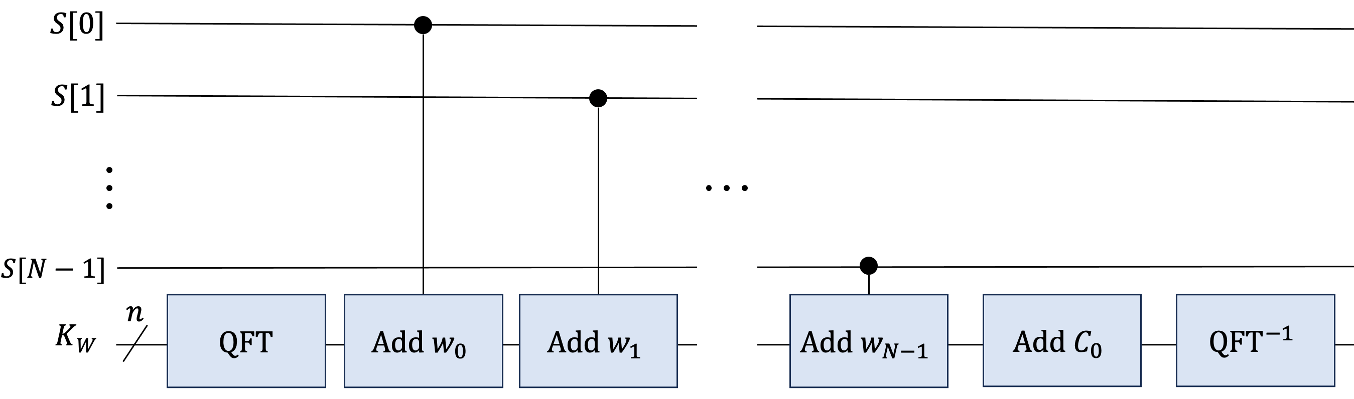
Figure 2: Circuit implementation of $U_{1}$, which encodes the total weights of item selections into the ancillary register $K_{W}$ using quantum Fourier transform-based arithmetic, adding a predefined offset $C_{0}$ to facilitate subsequent feasibility checking.

Following the implementation of the unitary operation $U_{1}$, $U_{2}$ is described, which comprises a quantum circuit that conditionally modifies the state of an ancillary qubit in concerning the sum of weights represented in the register $K_{w}$. Referring to Equation 17, the ancillary qubit $\ket{y}$ underwent a state flip to signal a valid configuration when the total weight $w(x)$, augmented by a constant offset $C_{0}$ is less than the predefined threshold $C+C_{0}+1$. This transformation was executed through several multicontrolled NOT gates, where each gate was influenced by a qubit distinct from the weight register. The successful transition of the ancillary qubit’s state post $U_{2}$ signified a feasible solution, adhering to the knapsack’s capacity, which effectively segregates the solution space into permissible and impermissible weights.

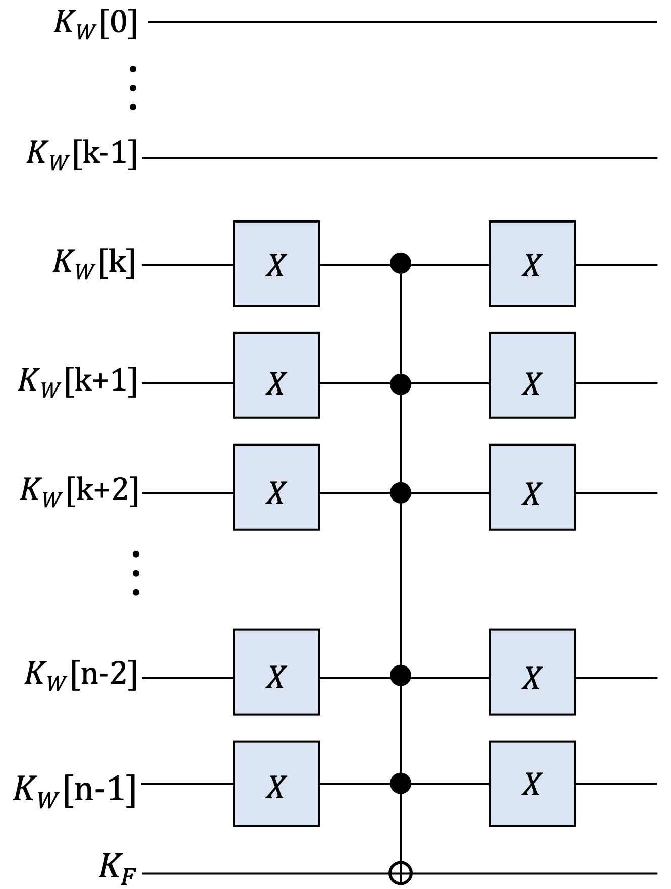
Figure 3: Circuit implementation of $U_{2}$, executing a conditional check based on the total weight calculated by $U_{1}$ using several multi-controlled NOT gates to flip the ancillary qubit if the weight condition is satisfied.

4.3.2 Quantum Walk Mixer for Enforcing Constraints

This process relies on the mixing operator $U_{B}(\beta)$ generated by mixing Hamiltonian $B$ from Equation 9 as follows:

$$U_{B}(\beta)=e^{-i\beta B},$$ (22)

Alternatively, by leveraging the feasible function $f$ in Equation 15 and neighboring states $n_{i}(x)$ for exploring the solution space, $B$ can be described as

$$B\ket{x}\ =\ \sum_{i\ =0}^{N-1}f_{i}(x)\ket{n_{i}(x)},\ \forall\ x\ \in K(N),$$ (23)

where $n_{i}(x)$ is the $i_{th}$ neighbor of $x$ ($x$ with $i_{th}$ bit flliped). Using this alternative representation, it is easy to observe that $\forall x,x^{\prime}\in K(N)$.

$$\bra{x}B\ket{x^{\prime}}=\begin{cases}1,&\text{if \quad Ham}(x,x^{\prime})=1\\ 0,&\text{otherwise}\end{cases},$$ (24)

where Ham$(x,x^{\prime})$ represents the Hamming distance between two binary strings $x$ and $x^{\prime}$, which is the count of positions where the corresponding bits differ. The exact implementation of the desired mixing operator $U_{B}(\beta)$ presents challenges due to its Hamiltonian, requiring additional resources and noncommuting elements. To address this, we employ an alternative operator $\tilde{B}$, closely resembling $B$. This operator is constructed from $V_{i}$, and the inverse $V_{i}^{\dagger}$ for encoding feasibility information of neighboring states into auxiliary qubits that enable the controlled state manipulation. Additionally, the operator includes single-qubit $X_{i}$ gates for creating neighboring state exploration. Moreover, $U_{f}$—the feasible oracle—is included to determine the feasibility of states by ensuring that only valid states are mixed. Finally, $R_{i}^{X}(2\beta)$ aids in adjusting the amplitudes of states based on feasibility and further refining the mixing process, whereas auxiliary qubits are employed to store feasibility information.

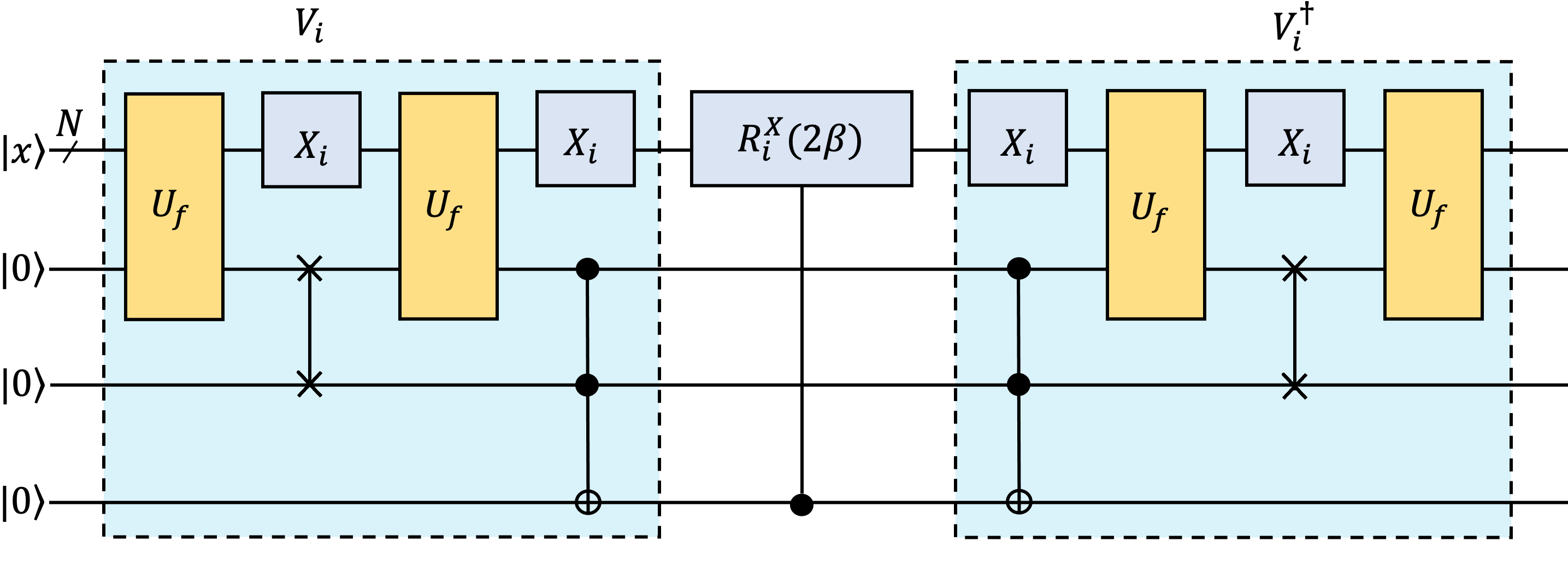
Figure 4: General circuit for a single-qubit quantum walk mixer illustrating the core operations involved in mixing a quantum state with its feasible neighbor, guided by feasibility oracles and single-qubit rotations, as part of a constrained optimization algorithm.

As shown in Figure 4, the process starts from:

$$\begin{array}[]{l}V_{i}V_{i}^{\dagger}\ket{x,0,0,0}\ =\ \ket{x,0,0,0},\end{array}$$ (25)

which implies that the behavior of $V_{i}$ when acting on a state $\ket{x,0,0,0}$ is to transform it into a new state with additional information encoded in the auxiliary qubits, dependent on the feasibility function $f$ and its value at neighboring points. Therefore, the state of $V_{j}$ can be described as

$$V_{i}\ket{x,0,0,0}=\ket{x,f(n_{i}(x)),f(x),f_{i}(x))}.$$ (26)

Next, neighboring state mapping is performed using $V_{i}^{\dagger}$ to determine whether the original and neighboring states have the same feasibility. Thus, Equation 25 can be written as

$$\begin{array}[]{l}V_{i}^{\dagger}\ket{x,f(n_{i}(x)),f(x),\ f_{i}(x))}\\[8.0pt] =\ket{n_{i}(x),f(x)\oplus f(n_{i}(x)),f(x)\oplus f(n_{i}(x)),f_{i}(x)\oplus f_{i}(x)}\\[8.0pt] =\begin{cases}\ket{n_{i}(x),0,0,0},\quad\text{if}\quad f(x)=f(n_{i}(x))\\ [8pt]\ket{n_{i}(x),1,1,0},\quad\text{otherwise}\end{cases}.\end{array}$$ (27)

Then, the bit flip of the $i-{th}$ qubit acts as:

$$X_{i}\ket{x}=\ket{n_{i}(x)}.$$ (28)

Therefore, we can describe the encoded feasibility information after applying $V_{i}$ and based on Equation 26 as follows:

$$\begin{array}[]{l}(X_{i}\otimes\mathbb{I}{{}^{\otimes}}^{2}\ \otimes\ \ket{1}\bra{1})V_{i}\ket{x,0,0,0}\\[8.0pt] =f_{i}(x)\ket{n_{i}(x),f(n_{i}(x)),f(x),f_{i}(x)}.\end{array}$$ (29)

Next,

$$\begin{array}[]{l}V_{i}^{\dagger}\left(X_{i}\ \otimes\mathbb{I}{{}^{\otimes}}^{2}\ \otimes\ \ket{1}\bra{1}\right)V_{i}\ket{x,0,0,0}\\[8.0pt] =\ f_{i}(x)\ket{n_{i}(x),0,0,0}.\end{array}$$ (30)

Thus, for a given $\tilde{B}$ operator, which approximates the original $B$ operator, we have

$$\tilde{B}\ =\sum_{i=0}^{N-1}V_{i}^{\dagger}\left(X_{i}\ \otimes\mathbb{I}{{}^{\otimes}}^{2}\ \otimes\ \ket{1}\bra{1}\right)V_{i}.$$ (31)

Moreover, $\tilde{B}$ implements $B$ given three ancillary qubits, or more precisely, it is represents as:

$$\begin{array}[]{l}\tilde{B}\ket{x,0,0,0}=\sum_{i=0}^{N-1}f_{i}(x)\ket{n_{i}(x),0,0,0}\\[6.0pt] =B\otimes\mathbb{I}^{\otimes^{3}}\ket{x,0,0,0}\quad\forall x\in K(N).\end{array}$$ (32)

It follows that

$$\begin{array}[]{l}e^{-i\beta\tilde{B}}\ket{x,0,0,0}=e^{-i\beta B\otimes\mathbb{I}^{\otimes^{3}}\ket{x,0,0,0}}\\[7.0pt] =U_{B}(\beta)\otimes\mathbb{I}^{\otimes 3}\ket{x,0,0,0}.\end{array}$$ (33)

where $\tilde{B}$ is used to generate $U_{B}$. Moreover, $\tilde{B}$ is not commute and should use three ancilla qubits. Therefore, the approximate implementation of $e^{-i\beta\tilde{B}}$ needs to use the trotter product formula. Meanwhile, using the identity $R_{i}^{X}(2\beta)$, the state representing the rest of the circuit in Figure 4 is given by

$$\begin{array}[]{l}e^{-i\beta V_{i}^{\dagger}\left(X_{i}\ \otimes\mathbb{I}{{}^{\otimes}}^{2}\ \otimes\ \ket{1}\bra{1}\right)V_{i}}\\[3.0pt] =\ V_{i}^{\dagger}\left(R_{i}^{X}(2\beta)\otimes\mathbb{I}^{\otimes 2}\otimes\ \ket{1}\bra{1}+\mathbb{I}^{\otimes(N+2)}\otimes\ket{0}\bra{0}\right)V_{i}\end{array}$$ (34)

where $R_{i}^{X}(2\beta)=cos(\beta)\mathbb{I}^{\otimes N}-isin(\beta)X_{i}$. Furthermore, we optimized $U_{B}(\beta)\otimes\mathbb{I}^{\otimes 3}$ with the trotter product formula as

$$\begin{array}[]{l}e^{-\beta\tilde{B}}=(\prod_{i=0}^{N-1}V_{j}^{\dagger}(R_{i}^{X}(2\beta/m)\otimes\mathbb{I}^{\otimes 2}\\[6.0pt] \otimes\ket{1}\bra{1}+\mathbb{I}^{\otimes(N+2)}\otimes\ket{0}\bra{0})V_{j}k)^{m}+O\left(\frac{N\beta^{2}}{m}\right).\end{array}$$ (35)

Moreover, to maintain $\beta$ the validity of the approximation within the new parameter range, the $\beta$ range needs to be adjusted accordingly to $\beta\in[0,m\pi)$.

As an objective function, we use the value function $v$. Therefore, the corresponding phase separation can be described as follows:

$$U_{C}(\gamma)\ket{x}=e^{-i\gamma v(x)}\ket{x}.$$ (36)

4.3.3 Number of Qubit Requirements

The presented illustration implies that using a feasibility oracle with nf ancilla qubits requires $N+n_{f}+3$ qubits. In contrast, there is an exigency for an additional three qubits, specifically for generating the unitary $U_{B}$ (Equation 33).

5 Evaluation

This section presents the numerical results by evaluating the effectiveness of the proposed algorithm across different asset numbers along with the impact of parameter configuration.

5.1 Experimental Setup

Initially, we implemented the proposed method using the Qiskit library (Aleksandrowicz et al. 2019), a widely used open-source quantum computing framework. We run the algorithms on the QASM simulator, a tool provided by Qiskit for simulating quantum circuits, which helped us gain insights into the behavior and performance of the algorithms before moving on to the real quantum device. While using the real device, we used IBM Cairo, a 27-qubit quantum device, for quantum computations, which offers the opportunity to test the algorithms in a real-world quantum computing environment. The experimental phase involves conducting several tests in which we select varying stocks from well-known companies, such as Apple Inc. (AAPL), Amazon.com Inc. (AMZN), Alphabet Inc. (GOOGL), Microsoft Corporation (MSFT), NVIDIA Corporation (NVDA), and Tesla, Inc. (TSLA). Notably, the selection of these stocks was based on different scenarios, including cases with two, three, four, and five stocks. Postselection, we proceeded with the experimental setup of the proposed method. During the optimization process, we focused on optimizing QAOA, which was achieved by optimizing the $2p$ angle parameters, i.e., $\beta$ and $\gamma$, using the classical optimizer SHGO (Endres et al. 2018). Additionally, we integrated quantum walk to boost optimization by leveraging its benefits for refining the process and achieving superior results. To evaluate the performance of the proposed method, we defined the problem of our algorithm based on the number of assets to be optimized (Table 1). First, we selected 2–5 subsets of stocks using the capabilities of PyPortfoliopt (Martin. 2021). The values in Table 1 represent the expected return of stocks counting from January 1, 2018, to January 1, 2023. This step clarifies the problem and enables us to tailor our algorithm accordingly. We aimed to evaluate the effectiveness of the QAOA optimization technique concerning portfolio optimization. To achieve this, we specifically evaluated the performance of the algorithm using the best-known solution (BKS), a result of using a classical algorithm (Martello et al. 1999), where $1$ signifies selection and $0$ denotes exclusion. This technique compared the results obtained from our algorithm with those of the classical solution, providing a benchmark for assessing its performance and effectiveness. By undertaking this evaluation, we can gain valuable insights into the capabilities and limitations of the QAOA optimization technique in portfolio optimization.

Table 1: Preparation for the portfolio optimization model uses expected returns based on the Markowitz model, as values in a knapsack problem, along with a key constraint. Capacity, set at $1$ or $2$, limits the stocks to $1$ or $2$, respectively. The model includes a classical solution best-known solution for comparing performance and specifies the number of qubits used in each stock selection scenario.

# Stocks	Type	Values	Capacity	BKS	Qubits
2	MSFT AAPL	0.26930 0.2488	1	(1,0)	7
3	MSFT AAPL NVDA	0.2315 0.2208 0.3638	1	(1,0,0)	8
4	MSFT AAPL GOOGL NVDA	0.2089 0.1984 0.2037 0.3220	2	(1,1,0,0)	10
5	MSFT AAPL GOOGL AMZN NVDA	0.1858 0.1941 0.1777 0.1826 0.2834	2	(0,1,0,0,1)	11

5.2 Performance Evaluation

By meticulously exploring the variable settings within the QWM-QAOA, we identified a circuit layer of $p=5$ and a trotter step value of $m=5$ as the optimal configuration for achieving superior results. Contextually, we explore the probability distributions arising for each stock in the portfolio. Figure 5 shows the experimental results, which are the optimal results of each scenario of the number of stocks. The obtained results reveal the probability distribution results for all possible cases of stock selection. Additionally, we employed the BKS method to evaluate the obtained results and ensured its expected behavior (Table 1).

Within the circuit layer of $5$, the approximation ratio varied based on the number of stocks in the portfolio. The obtained results ranged from 100% to 98% in a noiseless environment, from 98% to 80% when the fake backend was used, and from 49% to 33% when the real device was employed. When we extended our study to real-world conditions by implementing the experiment on the IBM Cairo device, the approximation ratio decreased to approximately 50% because of gate errors and decoherence affecting the fidelity of quantum states (Johnstun and Van Huele. 2021). Addressing these challenges will require additional efforts, such as error mitigation, which is beyond the scope of this study (Alam et al. 2019; Gaur et al. 2023).

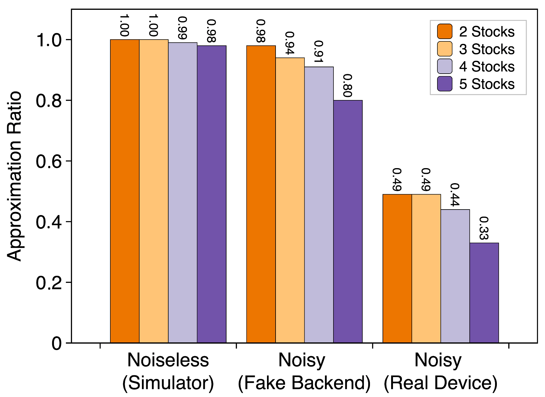
Figure 5: Probabilities for different scenarios involving various numbers of stocks under three distinct environmental conditions: noiseless, noisy with FakeCairoV2, and noisy with the ibm_cairo device.

5.2.1 Sensitivity Analysis

We conducted a comprehensive sensitivity analysis of key parameters using the QWM–QAOA algorithm. Our empirical exploration encompassed crucial elements, such as the circuit layer $(p)$ and the number of trotter steps $(m)$. These parameters are crucial for shaping the effectiveness of the proposed algorithm, and variation comprehension of their sensitivity is crucial for optimizing the performance of the algorithm. Through a methodical examination and evaluation, we present details of the relationship between these parameters and how much they influence the overall efficiency and resilience of QAOA.

• Circuit layer: Figure 6 shows that as the circuit layer increases beyond the initial value of $p\geqslant 3$, the approximation ratio of the diverse portfolio optimization result consistently reaches an impressive result ranging from from 100% to 98%, categorically based on the setup cases of portfolio optimization. This empirical evidence emphatically establishes that our performance consistently produces an efficient result even at some circuit layers.

  

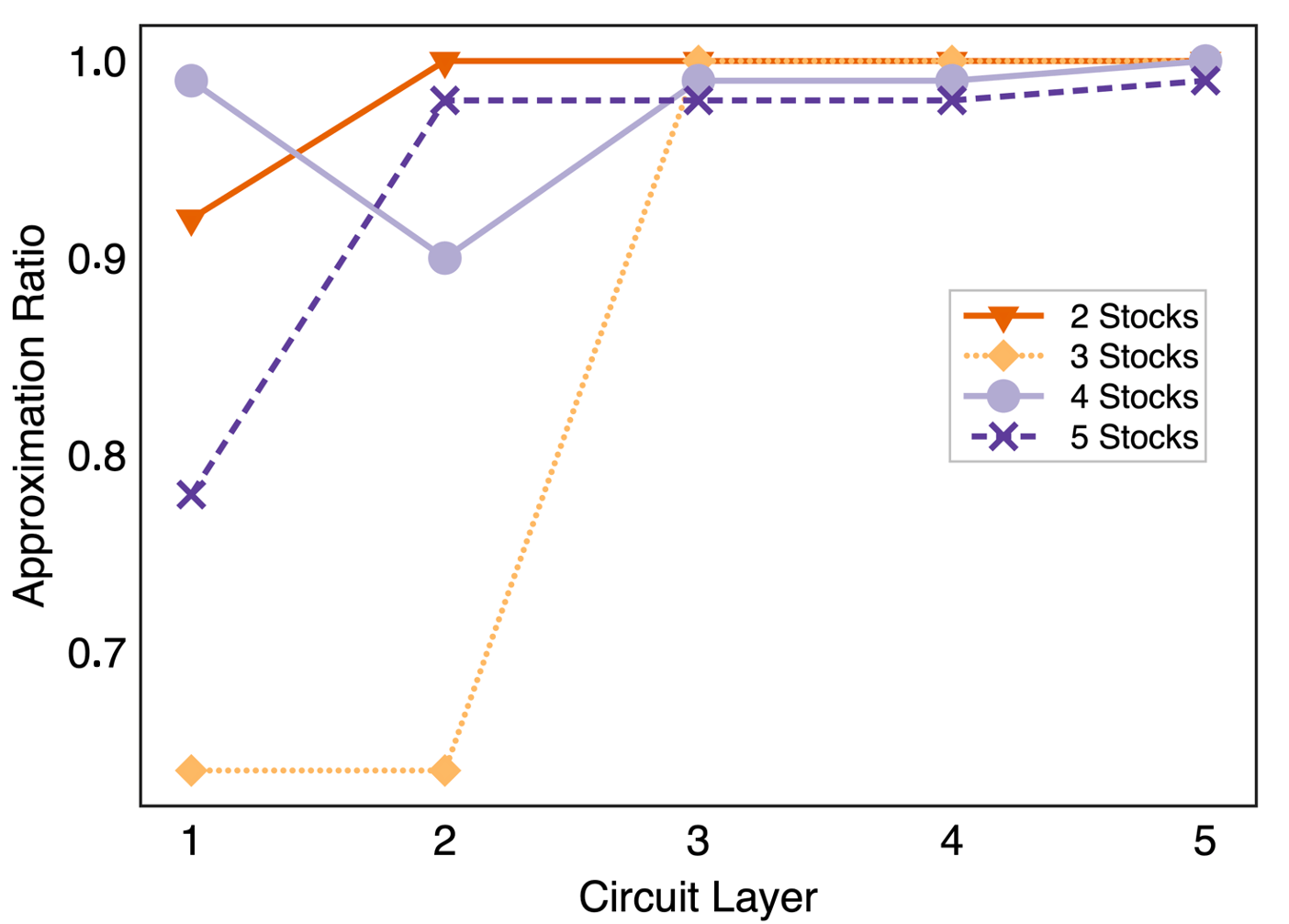
  Figure 6: Approximation ratio of the circuit layer$(p)$ is $1$–$5$ across all problems. Remarkably, when the$p\geqslant 3$, the approximation ratio reaches 100%, indicating that the proposed method is efficient even at the lower circuit layer.

• Trotter step count in QWM-QAOA: We aimed to find the parameter $m$, representing the trotter step counts in the QWM–QAOA algorithm while maintaining a constant circuit layer of $p=3$ and optimize $\beta$, $\gamma$ for the resulting circuit of $1$–$5$. Table 2 shows that the approximation ratio for various stock selections increasingly exhibits a better result starting from $m=3$, ranging from 99% to 97%. Finally, when $m=5$, we obtained an efficient optimization results from our proposed method ranging from 100% to 98%.

  Table 2: Number of trotters step $(m)$ of QWM–QAOA from $1$ to $5$, followed by the corresponding approximation ratio; results emphasize the importance of careful consideration when selecting the trotter step count, as it can significantly impact the approximation ratio.

  # Stocks	$m$ =1	$m$=2	$m$=3	$m$=4	$m$=5
  2	1	1	0.99	1	1
  3	0.99	0.61	0.99	0.99	1
  4	0.99	0.99	0.99	0.99	0.99
  5	0.80	0.97	0.97	0.98	0.98

6 Discussion and Conclusion

We empirically investigate the effectiveness of quantum computing techniques in portfolio optimization. We transform the portfolio optimization problem into a knapsack-based portfolio optimization and employ QWM–QAOA as the optimization method. Table 1 summarizes the data, including the number of stocks and required qubits, and outlines the direct relationship between stock count and qubit requirements. Furthermore, we compared our results with those of conventional optimization BKS to ensure the accuracy of our optimal solution. Optimization was performed under three different scenarios (Figure 5). Our proposed method achieves efficient results in noiseless and fake device settings, ranging from100% to 98% and 98% to 80%. However, in noisy real device conditions, the fidelity notably drops to approximately 50%, ranging from 50%, due to errors, indicating the potential for further research in error mitigation techniques. Moreover, we investigated the effectiveness of the proposed method using circuit layer analysis (Figure 6). The proposed method yields a result of 100% to 98% with $p\geqslant 3$ from various portfolio optimization scenarios and $2$–$5$ stocks. Table 2 emphasizes the critical role of selecting the number of trotter set counts $(m)$ in QWM–QAOA optimization. Consequently, with $m=5$, our approximation ratio reaches an impressive value between 100% and 98%.

Finally, by extending the experimentation to larger stock configurations of $2$–$5$ in the case of knapsack-based portfolio optimization using the QWM–QAOA technique, we aim to contribute valuable insights into the applicability and efficiency of the proposed approach across a broader spectrum of portfolio sizes. This research augments our understanding of the capacity of quantum computing. In particular, our proposed method improves portfolio optimization, especially concerning the knapsack-based problem and financial domain. In the future, we intend to extend the proposed method using large data by designing an error mitigation technique to enhance the potential of our current work.