Quasidiscrete spectrum Cherenkov radiation by a charge moving inside a dielectric waveguide
Abstract
We investigate the Cherenkov radiation by a charge uniformly moving inside a dielectric cylindrical channel in a homogeneous medium. The expressions for the Fourier components of the electric and magnetic fields are derived by using the electromagnetic field Green tensor. The spectral distribution of the Cherenkov radiation intensity in the exterior medium is studied for the general case of frequency dispersion of the interior and exterior dielectric functions. It is shown that, under certain conditions on the dielectric permittivities, strong narrow peaks appear in the spectral distribution. The spectral locations of those peaks are specified and their heights and widths are estimated analytically on the base of the dispersion equation for the electromagnetic eigenmodes of the cylinder.
1 Introduction
For many years after the discovery of Cherenkov radiation (CR, for review see [1]), it remains an active subject of theoretical and experimental investigations. The interest in CR is motivated by its applications as a high-power source of electromagnetic radiation in various frequency ranges, as well as related to a wide variety of applications in high-energy physics and materials science. The recent advances in the fields of metamaterials, nanophysics and photonic crystals open an interesting possibility to design materials having specified electromagnetic properties with controllable dispersion relations for effective dielectric permittivity and magnetic permeability. This provides an effective mechanism to control the characteristics of CR. Different guiding structures have been used for the further control of the radiation energy spectral-angular distributions. They include planar, cylindrical and spherical interfaces between two media with different electrodynamical properties (references for early investigations can be found in [1, 2]). More complicated structures require approximate and numerical methods for the investigation of the radiation features (see, for example, [3, 4, 5] and references therein).
In the present paper we consider the features of CR by a charged particle moving inside a cylindrical waveguide parallel to its axis. The various aspect of the energy losses of charged particles interacting with cylindrical interfaces have been discussed by many authors (see, e.g., [2, 3], [6]-[17], for a more complete list of references see [16, 17]). In particular, these interactions play an important role in particle accelerators. In addition of standard conducting and dielectric waveguides, as a realization of the cylindrical guiding structure we mention here the carbon nanotubes with radii tunable in relatively wide range.
The paper is organized as follows. In the next section we describe the problem setup and present the expressions for the Fourier components of the vector potential and for magnetic and electric fields. Assuming that the Cherenkov condition in the exterior medium is satisfied, in section 3 the formula is derived for the spectral density of the radiation, evaluating the energy flux through a cylindrical surface with large radius. The features of the radiation intensity are described depending on the relative permittivity. In section 4 the main results of the paper are summarized.
2 Electromagnetic fields
We consider a dielectric cylinder with permittivity embedded in a medium with dielectric permittivity . For the electromagnetic field source described by the current density the vector potential can be found by using the Green tensor , where and stands for the spacetime point . In the Lorentz gauge the corresponding relation reads
| (1) |
In the discussion below cylindrical coordinates with the axis along the cylinder axis will be used. The indices in (1) will correspond to the components , respectively. For the source of the radiation we will take the current density
| (2) |
with . It describes a point charge moving with constant velocity parallel to the axis of the cylinder. Denoting by the cylinder radius, we assume that .
Having the vector potential , the magnetic and electric fields and are found by the standard relations. It is convenient to present the discussion in terms of the partial Fourier components for the fields and Green tensor defined by
| (3) | |||||
| (4) |
with . From (1), the simple relation (to simplify the presentation we will omit the arguments of the Fourier components ) , is obtained for the components of the vector potential generated by the source (2).
By using the expressions for from [18] (see also [17]), we get
| (5) |
for the components and
| (6) |
for the axial component. Here, , , , , is the Bessel function and is the Hankel function of the first kind. Other notations are defined by the relations
| (7) | |||||
| (8) |
for and , . It is easily checked that the components (5) and (6) are continuous on the cylinder surface . The part of the field coming from the first term in the square brackets of (6) corresponds to the vector potential generated by the source (2) in a homogeneous medium with dielectric permittivity . The corresponding Fourier component is expressed as .
Given the vector potential, we can find the the magnetic and electric fields. Inside the cylinder, , the Fourier components of the fields are decomposed into two contributions:
| (9) |
with and for the magnetic and electric fields, respectively. The part corresponds to the field of a charged particle moving in an infinite homogeneous medium with permittivity and the contribution is induced by the difference of the permittivity in the region from . From the expression for given above, omitting the arguments , for the first contribution in (9) we get
| (12) | |||||
| (15) | |||||
| (16) |
with . For the contributions inside the cylinder we find
| (17) |
for . Here we have introduced the notation
| (18) |
For the Fourier components in the region one gets
| (19) |
where , and
| (20) |
3 Cherenkov radiation in the exterior medium
In this section we consider CR in the region assuming that the exterior medium is transparent and the dielectric permittivity is real. CR in the exterior medium is present under the condition corresponding to real values of . For the corresponding frequency one has and the radiation propagates along the Cherenkov angle with respect to the cylinder axis. The radial dependence of the Fourier components of the fields is expressed in terms of the Hankel functions and . For one has and the radial dependence is described by the Macdonald functions , with an exponential decrease of the Fourier components at large distances from the cylinder surface.
Assuming that , let us evaluate the energy flux per unit time through the cylindrical surface of radius coaxial with the dielectric cylinder. Denoting by the exterior unit normal to the surface, the flux is expressed in terms of the Fourier components as
| (21) |
By using the expressions (19) and the asymptotic of the Hankel functions for large arguments, the corresponding spectral density, defined by with , is presented in the form
| (22) | |||||
where , , and the prime on the summation sign means that the term should be taken with coefficient 1/2. The formula (22) is valid for general case of dispersions for dielectric permittivities and also for complex valued function . The dimensionless quantity is a function of , , and . The corresponding quantity for the radiation in a homogeneous medium with permittivity is obtained in the limit . In this limit one has , , and from (22) we get the standard expression .
In the special case of the motion along the cylinder axis one has and the only nonzero contribution in (22) comes from the mode . The general formula is reduced to
| (23) |
where .
For small values of the combination , , additionally assuming that , from (22) it can be seen that the contribution of the term with a given is proportional to and the dominant contribution comes from the term with . To the leading order, the radiation intensity coincides with that in a homogeneous medium with permittivity .
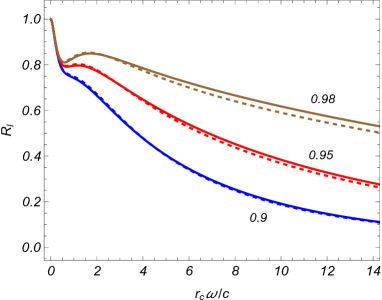
In figure 1, the ratio is plotted versus for . For the electron energy we have taken (full curves) and . For dielectric permittivity of the exterior medium the value is taken that corresponds to the dielectric permittivity for fused quartz in the frequency range . The graphs on the left and right panels are plotted for and , respectively. The second value corresponds to dielectric permittivity for teflon.
 |
|
In the numerical example presented in figure 1 we have taken real dielectric permittivities obeying the condition . In the corresponding spectral range the intensity is smaller than the one for CR in a homogeneous medium with permittivity . For the case corresponding to the left panel (the charge moves in a vacuum cylindrical hole), the CR is formed in the exterior medium. For the example on the right panel the Cherenkov condition is obeyed in both regions and and the spectral distribution of the CR intensity exhibits oscillations. Note that for relativistic velocities the dependence on the energy of the particles is relatively week.
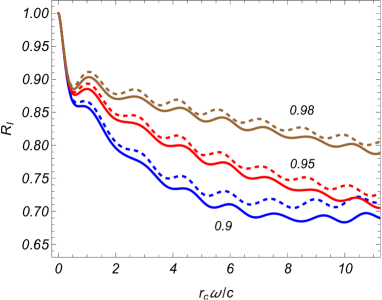
Figure 2 presents the spectral distribution of the ratio for and . As before, the full and dashed curves correspond to the particle energies and , respectively. We have taken for the left panel and for the right one. As seen from figure 2, in this case with , the strong narrow peaks appear in the spectral distribution of CR in the exterior medium for large values of .
 |
|
This feature of the radiation intensity distribution in the cylindrical setup under consideration has also been observed for a charge moving outside a cylinder [16] and in the spectral-angular distribution of the radiation by a charge circulating around or inside a cylinder [19, 20, 21]. The analytic explanation for the presence of the strong peaks seen in figure 2 is similar to that described in [16] and we shortly outline it assuming that both the media inside and outside the cylinder are transparent.
As noted above, the equation determines the eigenmodes of the dielectric cylinder. This equation has solutions under the condition with exponential suppression of the electromagnetic fields in the region at distances from the cylinder surface larger than the radiation wavelength. Two types of the eigenmodes correspond to guiding modes with (CR confined inside the cylinder) and to surface polaritons with . The modes of the second type are present under the condition and the corresponding radiation intensity has been investigated in [17] assuming that . For the function appearing in (22) is a complex function and has no zeros for real . However, that function can be exponentially small for large values of . The mathematical reason for that possibility is based on the fact that for large the ratio , with the Neumann function , is exponentially small for . Assuming that , for large we can expand the function over the small ratio of the Bessel and Neumann functions: , where
| (24) |
and . Now the function is real and at its possible zeros the function in (22) is of the order . Let us denote by the roots of the equation with respect to , where enumerates the roots for a given . Though these roots are not the eigenmodes of the dielectric cylinder, they obey the eigenmode equation with exponential accuracy. In this sense, we refer to those roots as quasimodes of the cylinder. We have checked numerically that the locations of the strong peaks in figure 2 coincide with with high accuracy. Note that the locations of the peaks do not depend on .
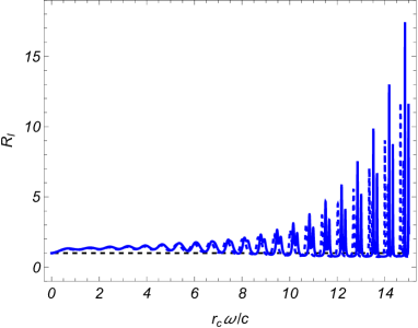
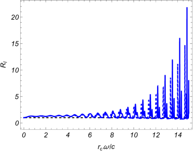
As it has been shown in [16], for the necessary condition for the existence of roots for the equation is reduced to which implies that . In the case , for the corresponding necessary condition one gets . By using the asymptotic expressions of the cylinder functions we can show that for the height of the peak for a given is proportional to the factor for . For the contribution of the term with a given to is proportional to the factor . By taking into account that the function is monotonically decreasing in the region , we conclude that in order to have a peak in the region the condition is required. The widths of the spectral peaks are obtained expanding the function near the roots and they are estimated as (see also [16]). The estimates for the characteristics of the spectral peaks were given under the assumption of real . For complex dielectric permittivity, in the expansion of the function near the roots additional terms appear proportional to the ratio , where and are the real and imaginary parts of . The estimates given above are valid in the range . For the case , the characteristics of the peaks in the spectral distribution are determined by the ratio . In addition to the decrease of the heigths, the inclusion of the imaginary part of dielectric permittivity leads to broadening of the peaks. The influence of several other factors, such as the finite length of the radiator and multiple scattering, has been discussed in [16] for .
4 Conclusion
We have described the features of radiation by a point charge moving inside a dielectric cylinder immersed in a homogeneous medium. The charge moves parallel to the cylinder axis at a constant velocity. Depending on the dielectric functions of the interior and exterior media and on the spectral range, three different types of polarization radiation can be emitted. They correspond to CR propagating in the exterior medium, CR confined inside the cylinder and surface polaritons confined near the cylinder surface. The radiation of the surface polaritons has been recently considered in [17] and here we were mainly concerned with CR in the exterior medium. The Fourier coefficients for the vector potential and for the electric and magnetic fields in both exterior and interior regions are determined by using the Green tensor from [18]. The spectral density of the intensity for CR in the exterior medium is given by the expression (22). The dependence of the radiation intensity on the distance of the charge trajectory from the axis of the cylinder enters through the function for a given . In the special case of motion along the cylinder axis the modes with contribute only and the general formula is further simplified to (23).
The spectral distribution of the radiation intensity for CR in the exterior medium essentially depends on the relation between the exterior and interior dielectric permittivities. The numerical results have been displayed for the ratio of spectral distributions in the presence of the cylinder and the corresponding quantity in a homogeneous medium with permittivity . For the case , that ratio is plotted in figure 1 and in the corresponding spectral range the presence of the cylinder leads to the decrease of the CR intensity compared to the radiation in a homogeneous medium. The situation can be essentially different in the case . As it is demonstrated by the example in figure 2, strong narrow peaks may appear in the spectral distribution of the radiation intensity. We have analytically argued the appearance of the peaks and estimated the corresponding heights and widths. The peaks come from the contribution of the modes with large and their locations coincide with the zeros of the function (24) with high accuracy.
We emphasize that the formula (22) is valid for the general case of the frequency dependence of the dielectric functions and and also for a complex function . It will be interesting to discuss the features described above for specific dispersion laws and also in the spectral ranges where . Another direction of investigations corresponds to the study of CR confined inside the cylinder. That radiation is emitted on the guiding modes of the cylinder being the solutions of the equation in the spectral range corresponding to . These investigations will be presented elsewhere.
Acknowledgement
The work was supported by the Higher Education and Science Committee of RA, in the frames of the projects 21AG-1C047 (A.A.S.) and 21AG-1C069 (L.Sh.G. and H.F.K.).
References
- [1] G.N. Afanasief, Vavilov-Cherenkov and Synchrotron Radiation, Springer, The Netherlands (2004).
- [2] B.M. Bolotovskii, Theory of Cherenkov radiation (III), Sov. Phys. Uspekhi 4 (1962) 781.
- [3] F.J. García de Abajo, Optical excitations in electron microscopy, Rev. Mod. Phys. 82 (2010) 209.
- [4] F.J. García de Abajo, A. Rivacoba, N. Zabala and N. Yamamoto, Boundary effects in Cherenkov radiation, Phys. Rev. B 69 (2004) 155420.
- [5] A.V. Tyukhtin, S.N. Galyamin and V. V. Vorobev, Peculiarities of Cherenkov radiation from a charge moving through a dielectric cone, Phys. Rev. A 99 (2019) 023810.
- [6] D. De Zutter and D. De Vleeschauwer, Radiation from and force acting on a point charge moving through a cylindrical hole in a conducting medium, J. Appl. Phys. 59 (1986) 4146.
- [7] N. Zabala, A. Rivacoba and P.M. Echenique, Energy loss of electrons travelling through cylindrical holes, Surf. Sci. 209 (1989) 465.
- [8] C.A. Walsh, An analytical expression for the energy loss of fast electrons traveling parallel to the axis of a cylindrical interface, Philos. Mag. B 63 (1991) 1063.
- [9] J.M. Pitarke and A. Rivacoba, Electron energy loss for isolated cylinders, Surf. Sci. 377-379 (1997) 294 . Y.-N. Wang and Z.L. Mišković, Energy loss of charged particles moving in cylindrical tubules, Phys. Rev. A 66 (2002) 042904.
- [10] G. Andonian et al., Resonant excitation of coherent Cerenkov radiation in dielectric lined waveguides, Appl. Phys. Lett. 98 (2011) 202901.
- [11] A.S. Kotanjyan, A.R. Mkrtchyan, A.A. Saharian and V.Kh. Kotanjyan, Radiation of surface waves from a charge rotating around a dielectric cylinder, JINST 13 (2018) C01016.
- [12] A.S. Kotanjyan, A.R. Mkrtchyan, A.A. Saharian, and V.Kh. Kotanjyan, Generation of surface polaritons in dielectric cylindrical waveguides, Phys. Rev. Spec. Top. Accel. Beams 22 (2019) 040701.
- [13] S.N. Galyamin, A.V. Tyukhtin, V.V. Vorobev, A.A. Grigoreva and A.S. Aryshev, Cherenkov radiation of a charge exiting open-ended waveguide with dielectric filling, Phys. Rev. Spec. Top. Accel. Beams 22 (2019) 012801.
- [14] S. Jiang, W.Li, Z.He, R. Huang, Q. Jia, L. Wang and Y. Lu, High power THz coherent Cherenkov radiation based on a separated dielectric loaded waveguide, Nucl. Instrum. Meth. A 923 (2019) 45.
- [15] A.R. Mkrtchyan, L.S. Grigoryan, A.A. Saharian, A.H. Mkrtchyan, H.F. Khachatryan, and V.K. Kotanjyan, Self-amplification of radiation from an electron bunch inside a waveguide filled with periodic medium, JINST 15 (2020) C06019.
- [16] A.A. Saharian, L.Sh. Grigoryan, A.Kh. Grigorian, H.F. Khachatryan and A.S. Kotanjyan, Cherenkov radiation and emission of surface polaritons from charges moving paraxially outside a dielectric cylindrical waveguide, Phys. Rev. A 102 (2020) 063517.
- [17] A.A. Saharian, L.Sh. Grigoryan, A.S. Kotanjyan and H.F. Khachatryan, Surface polariton excitation and energy losses by a charged particle in cylindrical waveguides. Phys. Rev. A 107 (2023) 063513.
- [18] L.Sh. Grigoryan, A.S. Kotanjyan and A. A. Saharian, Green function of an electromagnetic field in cylindrically symmetric inhomogeneous medium, Izv. Nats. Akad. Nauk Arm., Fiz. 30 (1995) 239 (Engl. Transl.: J. Contemp. Phys.).
- [19] A.A. Saharian and A.S. Kotanjyan,Synchrotron radiation from a charge moving along a helical orbit inside a dielectric cylinder, J. Phys. A 38 (2005) 4275.
- [20] A.A. Saharian and A.S. Kotanjyan, Synchrotron radiation from a charge moving along a helix around a dielectric cylinder, J. Phys. A 42 (2009) 135402.
- [21] A.S. Kotanjyan and A.A. Saharian, Undulator radiation inside a dielectric waveguide, Nucl. Instrum. Meth. B 309 (2013) 177.