Towards Quantifying the Preconditioning Effect of Adam

Abstract

There is a notable dearth of results characterizing the preconditioning effect of Adam and showing how it may alleviate the curse of ill-conditioning – an issue plaguing gradient descent (GD). In this work, we perform a detailed analysis of Adam’s preconditioning effect for quadratic functions and quantify to what extent Adam can mitigate the dependence on the condition number of the Hessian. Our key finding is that Adam can suffer less from the condition number but at the expense of suffering a dimension-dependent quantity. Specifically, for a $d$-dimensional quadratic with a diagonal Hessian having condition number $\kappa$, we show that the effective condition number-like quantity controlling the iteration complexity of Adam without momentum is $\mathcal{O}(\min(d,\kappa))$. For a diagonally dominant Hessian, we obtain a bound of $\mathcal{O}(\min(d\sqrt{d\kappa},\kappa))$ for the corresponding quantity. Thus, when $d<\mathcal{O}(\kappa^{p})$ where $p=1$ for a diagonal Hessian and $p=1/3$ for a diagonally dominant Hessian, Adam can outperform GD (which has an $\mathcal{O}(\kappa)$ dependence). On the negative side, our results suggest that Adam can be worse than GD for a sufficiently non-diagonal Hessian even if $d\ll\mathcal{O}(\kappa^{1/3})$; we corroborate this with empirical evidence. Finally, we extend our analysis to functions satisfying per-coordinate Lipschitz smoothness and a modified version of the Polyak-Łojasiewicz condition.

1 Introduction

Adaptive methods such as Adam (Kingma and Ba,, 2014) are often favored over (stochastic) gradient descent in training deep neural networks. There are some papers theoretically showing certain kinds of meaningful benefits of adaptive methods from the optimization perspective; for instance, with sparse gradients (Duchi et al.,, 2011; Zhou et al.,, 2018), exhibiting robustness to saddle points (Staib et al.,, 2019; Antonakopoulos et al.,, 2022), easier tuning of hyper-parameters (Faw et al.,, 2022, 2023; Wang et al.,, 2023), exhibiting robustness to unbounded smoothness (Crawshaw et al.,, 2022; Faw et al.,, 2023; Wang et al.,, 2022), etc. We survey related work in more detail in Section 2. However, given that the most widely used adaptive method, namely, Adam (update rule stated in Section 3) is frequently motivated as an adaptive diagonal preconditioner, there is a conspicuous absence of results characterizing its preconditioning effect, let alone demonstrating any benefits with respect to the condition number in any setting. In this work, we seek to quantify the preconditioning effect of Adam with exact gradients (i.e., in the deterministic setting) and answer the following question:

“Compared to gradient descent, how much better can Adam perform in terms of dependence on the condition number?”

Quadratic functions have a fixed Hessian, and so they are a natural first step to understand the preconditioning effect of Adam – given that there seem to be no results on this in any setting. We focus on $d$-dimensional quadratics of the form:

$$f(\bm{x})=\frac{1}{2}(\bm{x}-\bm{x}_{*})^{\top}\bm{Q}(\bm{x}-\bm{x}_{*}),$$ (1)

where $\bm{x},\bm{x}_{*}\in\mathbb{R}^{d}$ and the Hessian $\bm{Q}\in\mathbb{R}^{d\times d}$ is symmetric positive-definite. Note that $\nabla f(\bm{x})=\bm{Q}(\bm{x}-\bm{x}_{*})$ and $\text{arg min}_{\bm{x}\in\mathbb{R}^{d}}f(\bm{x})=\bm{x}_{*}$. Let $\bm{D}$ be the diagonal matrix containing the diagonal elements of $\bm{Q}$. Also, let the eigen-decomposition of $\bm{Q}$ be $\bm{U}\bm{\Lambda}\bm{U}^{\top}$; here $\bm{U}$ is a unitary matrix containing the eigenvectors of $\bm{Q}$ and $\bm{\Lambda}$ is a diagonal matrix containing the corresponding eigenvalues of $\bm{Q}$. Let $\kappa$ be the condition number of $\bm{Q}$ (i.e., the ratio of the maximum and minimum eigenvalues of $\bm{Q}$). It is well known in the literature that the iteration complexity of gradient descent (without momentum) scales as $\widetilde{\mathcal{O}}(\kappa)$; this can be prohibitive when $\kappa$ is extremely large or the Hessian is “ill-conditioned”. A key message of our paper is that Adam can suffer less from $\kappa$ but at the expense of suffering a quantity depending on the dimension $d$. With this preface, we will now state our main results and contributions.
1. In Theorem 2, we show that for diagonal $\bm{Q}$, the iteration complexity of Adam is $\widetilde{\mathcal{O}}\big{(}\min(d,\kappa)\big{)}$ with constant probability (e.g., ${3}/{4}$) over random initialization. So when $d<\mathcal{O}(\kappa)$, Adam can outperform gradient descent (GD) with constant probability.
2. Let $\overline{\kappa}$ be the condition number of $\bm{D}^{-1/2}\bm{Q}\bm{D}^{-1/2}$; this a diagonally preconditioned version of $\bm{Q}$ known as Jacobi preconditioning (Demmel,, 1997; Wathen,, 2015). Also, let $\kappa_{\text{diag}}$ be the condition number of $\bm{D}$; this is just the ratio of the maximum and minimum diagonal elements of $\bm{Q}$ and it is $\leq\kappa$. In Theorem 3 and the discussion after it, we show that for general (non-diagonal) $\bm{Q}$, the complexity of Adam is $\widetilde{\mathcal{O}}\big{(}\min\big{(}d\overline{\kappa}\sqrt{d\overline{\kappa}\kappa_{\text{diag}}},\overline{\kappa}\kappa_{\text{diag}}\big{)}\big{)}$ with constant probability over random initialization. So when $d<\mathcal{O}\big{(}\frac{1}{\overline{\kappa}}\big{(}\frac{\kappa^{2}}{\kappa_{\textup{diag}}}\big{)}^{{1}/{3}}\big{)}$, Adam can outperform GD with constant probability.
3. For diagonally dominant $\bm{Q}$ (see Definition 1), we show that $\overline{\kappa}=\mathcal{O}(1)$ and $\kappa=\mathcal{O}(\kappa_{\textup{diag}})$ in Theorem 4. So for such $\bm{Q}$, Adam can outperform GD when $d<\mathcal{O}\big{(}{\kappa^{1/3}}\big{)}$.
4. On the negative side, our result suggests that when $\overline{\kappa}$ is large enough, which is possible for sufficiently non-diagonal $\bm{Q}$, Adam can be worse than GD; see the discussion right after Remark 5. We corroborate this with empirical evidence in Figure 1. Also somewhat surprisingly, we show that Adam may not converge to zero function value asymptotically. We characterize the asymptotic point(s) to which it may converge in Section 4.2.
5. In Section 5, we turn our attention to functions that satisfy per-coordinate Lipschitz smoothness (Definition 5) and a modified version of the Polyak-Łojasiewicz (PL) condition (Definition 6). As per Theorem 8 and the discussion in Remark 12, Adam can be better than GD when an initialization-dependent quantity which implicitly grows with the dimension is smaller than the ratio of the maximum and minimum per-coordinate smoothness constants.
Our main results for quadratic functions are summarized in Table 1; they are directly relevant to linear regression and wide deep neural networks that evolve as linear models (Lee et al.,, 2019), where the objective function is quadratic.
High-level overview of proof techniques: Key ingredients of our analysis include envisioning the evolution of Adam’s iterates as a “pseudo-linear” system (Remark 7), applying judicious manipulations to “cancel out” the effect of $\kappa$ as much as possible (Remark 8) and deriving a decay rate with a two-stage analysis procedure (Remark 9). We discuss the proof outline of Theorem 3 (result for general $\bm{Q}$) in Section 4.1.

Nature of Hessian $\bm{Q}$	Adam (w/o momentum)	GD
Diagonal	$\mathcal{O}\Big{(}\min(d,\kappa)\log(\frac{1}{\varepsilon})\log\log(\frac{1}{\varepsilon})\Big{)}$	$\mathcal{O}\Big{(}\kappa\log(\frac{1}{\varepsilon})\Big{)}$
Diagonally Dominant (Def. 1)	$\mathcal{O}\Big{(}\min\big{(}d\sqrt{d\kappa},\kappa\big{)}\log(\frac{1}{\varepsilon})\log\log(\frac{1}{\varepsilon})\Big{)}$	$\mathcal{O}\Big{(}\kappa\log(\frac{1}{\varepsilon})\Big{)}$
General	$\mathcal{O}\Big{(}\min\big{(}d\overline{\kappa}\sqrt{d\overline{\kappa}\kappa_{\text{diag}}},\overline{\kappa}\kappa_{\text{diag}}\big{)}\log(\frac{1}{\varepsilon})\log\log(\frac{1}{\varepsilon})\Big{)}$	$\mathcal{O}\Big{(}\kappa\log(\frac{1}{\varepsilon})\Big{)}$

Table 1: Iteration complexities of Adam w/o momentum and GD to converge to $\varepsilon$ error for minimizing $f(\bm{x})=\frac{1}{2}(\bm{x}-\bm{x}_{*})^{\top}\bm{Q}(\bm{x}-\bm{x}_{*})$ (eq. 1). Here $d$ is the dimension, $\kappa$ is the condition number of $\bm{Q}$, $\overline{\kappa}$ is the condition number of $\bm{D}^{-1/2}\bm{Q}\bm{D}^{-1/2}$ and $\kappa_{\text{diag}}\leq\kappa$ is the condition number of $\bm{D}$, where $\bm{D}$ is the diagonal matrix containing the diagonal elements of $\bm{Q}$. The results for Adam are with constant probability (e.g., $3/4$) over random initialization.

2 Related Work

There is copious amount of work on the convergence of adaptive gradient methods (Ward et al.,, 2020; Reddi et al.,, 2018; Chen et al.,, 2018; Zaheer et al.,, 2018; Zhou et al.,, 2018; Li and Orabona,, 2019; Huang et al.,, 2021; Da Silva and Gazeau,, 2020; Shi and Li,, 2021; Défossez et al.,, 2022; Zhang et al.,, 2022). Some papers show certain kinds of meaningful benefits of adaptive methods from the optimization perspective, and we focus on these papers. For e.g., adaptive methods can outperform non-adaptive methods when the gradients are sparse (Duchi et al.,, 2011; Zhou et al.,, 2018). Staib et al., (2019); Antonakopoulos et al., (2022) show that adaptive methods are robust to the presence of saddle points. Faw et al., (2022, 2023); Wang et al., (2023) show that setting hyper-parameters is easier for adaptive methods in the sense that we do not need to be privy to problem-dependent parameters such as the smoothness constant, noise variance, etc. Moreover, adaptive methods enjoy convergence even with unbounded smoothness (Crawshaw et al.,, 2022; Faw et al.,, 2023; Wang et al.,, 2022). Pan and Li, (2023) attempt to justify the success of adaptive methods over SGD in deep networks by empirically showing that the update direction of adaptive methods is associated with a much smaller directional sharpness value than SGD. Another rather weak motivation for the effectiveness of Adam is that it can approximately mimic natural gradient descent (Amari,, 1998); as pointed out by Martens, (2020); Balles and Hennig, (2018) there are issues with this view.

3 Preliminaries

Suppose we wish to minimize $f:\mathbb{R}^{d}\xrightarrow{}\mathbb{R}$ with access to exact gradients. Let $\bm{x}_{k}$ be the iterate of Adam in the $k^{\text{th}}$ iteration and let $\bm{g}_{k}=\nabla f(\bm{x}_{k})$. For each $i\in\{1,\ldots,d\}$, let

$${m}_{k}^{(i)}=\beta_{1}{m}_{k-1}^{(i)}+{g}_{k}^{(i)}\text{ with }{m}_{0}^{(i)}=0\text{ and }{v}_{k}^{(i)}=\beta_{2}{v}_{k-1}^{(i)}+\big{(}{g}_{k}^{(i)}\big{)}^{2}\text{ with }{v}_{0}^{(i)}=0,$$ (2)

where $\beta_{1},\beta_{2}\in(0,1)$ are known as the first moment/momentum and second moment hyper-parameters. Before stating the exact update rule that we analyze in this work, we will state its “nearest neighbor” to the vanilla version of Adam proposed by Kingma and Ba, (2014). For this nearest neighbor, the update rule of the $i^{\text{th}}$ coordinate in the $k^{\text{th}}$ iteration is:

$$x^{(i)}_{k+1}=x^{(i)}_{k}-\frac{\alpha{m}_{k}^{(i)}}{\sqrt{{v}_{k}^{(i)}+\delta}},$$ (3)

where $\alpha$ is the step-size and $\delta$ is a small correction term in the update’s denominator (to avoid division by zero). This is very closely related to the vanilla version of Adam proposed by Kingma and Ba, (2014); we discuss this close connection in Appendix A. For the variant that we propose and analyze, $\delta$ in eq. 3 is replaced by a coordinate-dependent and iteration-dependent term; it is as follows:

$$x^{(i)}_{k+1}=x^{(i)}_{k}-\frac{\alpha{m}_{k}^{(i)}}{\sqrt{v_{k}^{(i)}+\max\Big{(}\big{(}{g}_{0}^{(i)}\big{)}^{2},\phi^{2}\Big{)}\delta_{k}^{2}}}.$$ (4)

Note that $\delta$ in eq. 25 is replaced by $\max\big{(}\big{|}{g}_{0}^{(i)}\big{|},\phi\big{)}\delta_{k}$. It is worth pointing out that the coordinate-dependent $\delta$ that we set above plays a crucial role in improving the dependence with respect to the condition number (see Remarks 2 and 4).

Our results for Adam in this paper are without first moment/momentum, i.e., with $\beta_{1}=0$. The key difference of Adam from GD-style algorithms is the square root diagonal preconditioner involving the exponential moving average of squared gradients – this is the aspect that we focus on.

Also, recall the update rule of gradient descent (GD) with step-size $\alpha$ is $x^{(i)}_{k+1}=x^{(i)}_{k}-{\alpha{g}_{k}^{(i)}}$.

3.1 Notation

For any $n\in\mathbb{N}$, we define $[n]:=\{1,\ldots,n\}$. Vectors and matrices are in bold font. Let $\bm{e}_{i}$ denote the $i^{\text{th}}$ canonical vector, i.e., the vector of all zeros except a one in the $i^{\text{th}}$ coordinate. We denote the $i^{\text{th}}$ coordinate of a vector $\bm{v}\in\mathbb{R}^{p}$ by $v^{(i)}$, where $i\in[p]$. For a matrix $\bm{M}\in\mathbb{R}^{m\times n}$, we denote its $(i,j)^{\text{th}}$ element by $M[i,j]$, where $i\in[m]$ and $j\in[n]$. We denote the maximum and minimum singular values/eigenvalues of $\bm{M}$ by $\sigma_{\text{max}}(\bm{M})$ and $\sigma_{\text{min}}(\bm{M})$/$\lambda_{\text{max}}(\bm{M})$ and $\lambda_{\text{min}}(\bm{M})$, respectively. $\text{cond}(\bm{M})$ denotes the condition number of $\bm{M}$, i.e., $\frac{\sigma_{\text{max}}(\bm{M})}{\sigma_{\text{min}}(\bm{M})}$. We denote the Hadamard (i.e., element-wise) product of two matrices $\bm{A},\bm{B}\in\mathbb{R}^{m\times n}$ by $\bm{A}\circ\bm{B}$. $\textup{Unif}[a,b]$ denotes the uniform distribution over $[a,b]$.

3.2 Important Definitions

Refer to the problem setting in eq. 1. Recall that $\bm{U}\bm{\Lambda}\bm{U}^{\top}$ is the eigen-decomposition of $\bm{Q}$ and $\bm{D}$ is the diagonal matrix containing the diagonal elements of $\bm{Q}$ (i.e., $\bm{D}=\bm{Q}\circ\bm{\text{{I}}}$). We will define some important quantities here.

• Let $\lambda_{i}={\Lambda}[i,i]$ be the $i^{\text{th}}$ eigenvalue of $\bm{Q}$. Further, let $\lambda_{\max}(\bm{Q})=\kappa$ and $\lambda_{\min}(\bm{Q})=1$ for simplicity; so, $\text{cond}(\bm{Q})=\kappa$.

• Let $q_{i}=Q[i,i]=D[i,i]$ be the $i^{\text{th}}$ diagonal element of $\bm{Q}$ (and $\bm{D}$). Further, let $q_{\text{max}}=\max_{i\in[d]}q_{i}$ and $q_{\text{min}}=\min_{i\in[d]}q_{i}$. Also, define $\kappa_{\text{diag}}:=\big{(}\frac{q_{\text{max}}}{q_{\text{min}}}\big{)}$. Then, $\text{cond}(\bm{D})=\kappa_{\text{diag}}$. It holds that $\kappa_{\text{diag}}\leq\kappa$ with equality holding when $\bm{Q}$ is diagonal and equal to $\bm{D}$.

• Define $\bar{\bm{Q}}:=\bm{D}^{-1/2}\bm{U}\bm{\Lambda}^{1/2}$ and let $\text{cond}(\bar{\bm{Q}})=\sqrt{\overline{\kappa}}$. Note that $\bar{\bm{Q}}\bar{\bm{Q}}^{\top}=\bm{D}^{-1/2}\bm{Q}\bm{D}^{-1/2}$ and $\text{cond}(\bm{D}^{-1/2}\bm{Q}\bm{D}^{-1/2})=\text{cond}(\bar{\bm{Q}}\bar{\bm{Q}}^{\top})=\overline{\kappa}$.

• Define $\widehat{\bm{Q}}:=\bm{D}^{-1}\bm{U}\bm{\Lambda}^{1/2}=\bm{D}^{-1/2}\bar{\bm{Q}}$. Let $\sigma_{\text{min}}(\widehat{\bm{Q}})=\rho_{1}$ and $\sigma_{\text{max}}(\widehat{\bm{Q}})=\rho_{2}$. Also, define $\widehat{\kappa}:=\big{(}\frac{\rho_{2}}{\rho_{1}}\big{)}$. Then, $\text{cond}(\widehat{\bm{Q}})=\widehat{\kappa}$ and it holds that $\widehat{\kappa}\leq\sqrt{\kappa_{\text{diag}}\overline{\kappa}}$.

Observe that if $\bm{Q}$ is diagonal (in which case, $\bm{U}=\bm{\text{{I}}}$ and $\bm{Q}=\bm{D}=\bm{\Lambda}$), $\overline{\kappa}=1$, $\rho_{1}=\frac{1}{\sqrt{\kappa}}$, $\rho_{2}=1$ and hence, $\widehat{\kappa}=\sqrt{\kappa}=\sqrt{\kappa_{\text{diag}}}$. Also, $\bm{D}^{-1/2}\bm{Q}\bm{D}^{-1/2}$ is a diagonally preconditioned version of $\bm{Q}$ and this type of preconditioning is known as Jacobi preconditioning (Wathen,, 2015).

4 Main Results for Quadratic Functions

Here we will compare the convergence of Adam and GD (both without momentum) for quadratic functions. We first state the folklore iteration complexity of GD with step-size $\alpha={1}/{\kappa}$; recall that the step-size of GD must not exceed two times the inverse of the maximum eigenvalue of the Hessian to ensure convergence.

Theorem 1 (GD: Folklore).

Suppose our initialization is $\bm{x}_{0}$. Set $\alpha={1}/{\kappa}$. Then, $f(\bm{x}_{\widehat{K}})<\frac{\varepsilon^{2}}{2}$ in

$$\widehat{K}=\mathcal{O}\Big{(}{\kappa}\log\Big{(}\frac{\sqrt{\kappa}\|\bm{x}_{0}-\bm{x}_{*}\|_{2}}{\varepsilon}\Big{)}\Big{)}$$

iterations of GD.

Note that the iteration complexity of GD depends on the condition number of $\bm{Q}$, viz., $\kappa$. We shall state the corresponding iteration complexity of Adam (with $\beta_{1}=0$) for diagonal and general $\bm{Q}$ separately. Let us look at the diagonal case first.

Theorem 2 (Adam: Diagonal $\bm{Q}$).

Let $\bm{Q}=\bm{\Lambda}$ be diagonal. Suppose $\|\bm{x}_{*}\|_{\infty}\leq B$ and our initialization $\bm{x}_{0}$ is sampled randomly such that ${x}_{0}^{(i)}\underset{\textup{iid}}{\sim}\textup{Unif}[-2B,2B]$ $\forall$ $i\in[d]$. There exist $\alpha$, $\beta_{2}$, $\delta_{k}$ and $\phi$ such that with a probability of at least $p$ over the randomness of $\bm{x}_{0}$, $f(\bm{x}_{{K}^{*}})<\frac{\varepsilon^{2}}{2}$ in

$$K^{*}=\mathcal{O}\Bigg{(}\kappa_{\textup{Adam}}{\log\Big{(}\frac{\sqrt{d\kappa}B}{\varepsilon}\Big{)}{\log\Big{(}\log\Big{(}\frac{\sqrt{d\kappa}\|\bm{x}_{0}-\bm{x}_{*}\|_{\infty}}{\varepsilon}\Big{)}\Big{)}}}\Bigg{)}$$

iterations of Adam, where $\kappa_{\textup{Adam}}:=\min\Big{(}\frac{d}{\log(1/p)}+1,\kappa\Big{)}$.

The detailed version and proof of Theorem 2 can be found in Appendix D. Observe that the condition number-like quantity $\kappa_{\textup{Adam}}$ appearing in the iteration complexity of Adam is $\mathcal{O}(\min(d,\kappa))$ with constant probability (e.g., ${3}/{4}$).

It is true that the dependence on $\varepsilon$ for Adam is slightly worse than GD (Theorem 1). However, logarithmic dependence on $\nicefrac{{1}}{{\varepsilon}}$ is pretty benign and the problem-dependent constant factors multiplying the $\log(\nicefrac{{1}}{{\varepsilon}})$ and $\log(\nicefrac{{1}}{{\varepsilon}})\log\log(\nicefrac{{1}}{{\varepsilon}})$ terms for GD and Adam – viz., $\kappa$ and $\kappa_{\textup{Adam}}$ – dictate the overall convergence speed. Hence, we are interested in these problem-dependent constant factors and we ignore the dependence on $\varepsilon$ in all subsequent discussions.

Remark 1.

When $d<\mathcal{O}(\kappa)$, $\kappa_{\textup{Adam}}<\kappa$ with constant probability over the randomness of $\bm{x}_{0}$.

Remark 2.

The coordinate-dependent $\delta$ that we chose in eq. 4 is critical to $\kappa_{\textup{Adam}}$ being $\mathcal{O}(\min(d,\kappa))$. Specifically, without the $\big{(}{g}_{0}^{(i)}\big{)}^{2}$ terms, our bound for $\kappa_{\textup{Adam}}$ is $\mathcal{O}(\kappa)$.

Let us now move on to the case of general (non-diagonal) $\bm{Q}$. We begin by introducing an assumption on the nature of random initialization.

Assumption 1 (Random Initialization).

Let $\bm{T}=\bm{D}^{-1}\bm{Q}$ and $\|\bm{T}\bm{x}_{*}\|_{\infty}\leq B$. Our initialization $\bm{x}_{0}$ is sampled randomly such that each coordinate of $\bm{T}\bm{x}_{0}$ $\in[-2B,2B]$. Also, let $\widehat{\bm{g}}_{0}=\bm{T}(\bm{x}_{0}-\bm{x}_{*})$. For any $t\in[0,1]$, $\mathbb{P}\Big{(}\min_{i\in[d]}|\widehat{g}_{0}^{(i)}|>\frac{2tB}{d}\Big{)}\geq\exp\Big{(}-\frac{\zeta t^{\theta}}{1-\frac{\zeta t^{\theta}}{d}}\Big{)}$ for some $\theta\in(0,1]$ and $\xi\geq 1$.

The above assumption on the distribution of $\min_{i\in[d]}|\widehat{g}_{0}^{(i)}|$ is weaker than assuming each coordinate of $\bm{T}\bm{x}_{0}$ is drawn i.i.d. from $\textup{Unif}[-2B,2B]$. If we assumed the latter, then we would have $\mathbb{P}\Big{(}\min_{i\in[d]}|\widehat{g}_{0}^{(i)}|>\frac{2tB}{d}\Big{)}\geq\exp\Big{(}-\frac{t}{1-\frac{t}{d}}\Big{)}$ (see eq. 117 in the proof of Lemma 7) which is $\geq\exp\Big{(}-\frac{\zeta t^{\theta}}{1-\frac{\zeta t^{\theta}}{d}}\Big{)}$ for $t\in[0,1]$ as $\theta\in(0,1]$ and $\xi\geq 1$.

Ideally, we would have liked to derive results with $\bm{x}_{0}$ being sampled uniformly at random like the diagonal case (Theorem 2). Unfortunately, this seems difficult in general but when $\bm{Q}$ is close to diagonal, this is possible; we discuss these things in Appendix B.

Let us now look at the result for a general $\bm{Q}$ under 1.

Theorem 3 (Adam: General $\bm{Q}$).

Suppose our initialization $\bm{x}_{0}$ satisfies 1. Fix some $p\in[\frac{1}{e},1)$. There exist $\alpha$, $\beta_{2}$, $\delta_{k}$ and $\phi$ such that with a probability of at least $p$ over the randomness of $\bm{x}_{0}$, $f(\bm{x}_{{K}^{*}})<\frac{\varepsilon^{2}}{2}$ in

$$K^{*}=\mathcal{O}\Bigg{(}\kappa_{\textup{Adam}}\log\Big{(}\frac{\sqrt{d}B}{\rho_{1}\varepsilon}\Big{)}{\log\Big{(}\log\Big{(}\frac{\|\bm{\Lambda}^{1/2}{\bm{U}}^{\top}(\bm{x}_{0}-\bm{x}_{*})\|_{2}}{\varepsilon}\Big{)}\Big{)}}\Bigg{)}$$

iterations of Adam, where $\kappa_{\textup{Adam}}:=\overline{\kappa}\min\Big{(}\Big{(}\frac{\widehat{\kappa}d^{3/2}}{\log^{1/\theta}({1}/{p})}\Big{)}\zeta^{1/\theta}\big{(}1+\frac{\log(1/p)}{d}\big{)}^{1/\theta},\kappa_{\textup{diag}}\Big{)}$.

The detailed version and proof of Theorem 3 can be found in Appendix C; also see the discussion on hyper-parameters after the detailed version of Theorem 3. We discuss the proof outline of Theorem 3 in Section 4.1. Observe that the condition number-like quantity $\kappa_{\textup{Adam}}$ appearing in the iteration complexity of Adam above is $\mathcal{O}\big{(}\min\big{(}\overline{\kappa}\widehat{\kappa}d^{3/2},\overline{\kappa}\kappa_{\textup{diag}}\big{)}\big{)}$ with constant probability. Using the fact that $\widehat{\kappa}\leq\sqrt{\kappa_{\text{diag}}\overline{\kappa}}$, we have the following simpler bound for $\kappa_{\textup{Adam}}$:

$$\kappa_{\textup{Adam}}\leq\mathcal{O}\Big{(}\min\big{(}d\overline{\kappa}\sqrt{d\overline{\kappa}\kappa_{\text{diag}}},\overline{\kappa}\kappa_{\text{diag}}\big{)}\Big{)}.$$ (5)

So $\kappa_{\textup{Adam}}<\kappa$ when $\mathcal{O}\big{(}d\overline{\kappa}\sqrt{d\overline{\kappa}\kappa_{\text{diag}}}\big{)}<\kappa$. Simplifying this, we can make the following remark.

Remark 3.

When $d<\mathcal{O}\big{(}\frac{1}{\overline{\kappa}}\big{(}\frac{\kappa^{2}}{\kappa_{\textup{diag}}}\big{)}^{{1}/{3}}\big{)}$, $\kappa_{\textup{Adam}}<\kappa$ with constant probability over the randomness of $\bm{x}_{0}$. Further, since $\kappa_{\text{diag}}\leq\kappa$, a simpler but looser version of the previous condition is $d<\mathcal{O}\big{(}\frac{\kappa^{1/3}}{\overline{\kappa}}\big{)}$.

Remark 4.

Once again, the $\big{(}{g}_{0}^{(i)}\big{)}^{2}$ terms in the coordinate-dependent $\delta$ that we set in eq. 4 are crucial in obtaining the above improvement.

Value of $\overline{\kappa}$. Recall that $\overline{\kappa}=\text{cond}(\bm{D}^{-1/2}\bm{Q}\bm{D}^{-1/2})$ is the condition number of Jacobi-preconditioned $\bm{Q}$. In general, $\overline{\kappa}$ may not be “small”. To our knowledge, the best known bound for $\overline{\kappa}$ is $\overline{\kappa}\leq\kappa^{*}\min(\kappa^{*},d)$, where $\kappa^{*}=\min_{\text{diag. }\bm{\Sigma}\succeq 0_{d\times d}}\text{cond}(\bm{\Sigma}^{1/2}\bm{Q}\bm{\Sigma}^{1/2})$ (Jambulapati et al.,, 2020). When $\bm{Q}$ is diagonal (in which case it is equal to $\bm{D}$), $\overline{\kappa}=1$. Hence, we expect $\overline{\kappa}$ to be $\mathcal{O}(1)$ when $\bm{Q}$ is “sufficiently diagonal”. We formally quantify this in the diagonally dominant case (defined below) which is a relaxation of the perfectly diagonal case.

Definition 1 ($\nu$-diagonally-dominant).

A square matrix $\bm{P}\in\mathbb{R}^{n\times n}$ is said to be $\nu$-diagonally-dominant if for all $i\in[n]$, it holds that $\sum_{j\neq i}|P[i,j]|\leq\nu|P[i,i]|$ for some $\nu\in[0,1)$.

It is worth mentioning that the usual definition of diagonally dominant matrices in the literature is with $\nu=1$ above. Further, note that $\nu=0$ corresponds to the pure diagonal case.

Theorem 4.

Suppose $\bm{Q}$ is $\nu$-diagonally-dominant. Then $\bar{\kappa}\leq\big{(}\frac{1+\nu}{1-\nu}\big{)}$ and $\kappa\leq\big{(}\frac{1+\nu}{1-\nu}\big{)}\kappa_{\textup{diag}}$. So when $\nu$ is uniformly bounded below $1$, $\overline{\kappa}=\mathcal{O}(1)$ and $\kappa=\mathcal{O}(\kappa_{\textup{diag}})$.

We prove Theorem 4 in Appendix F.

Remark 5.

When $\bm{Q}$ satisfies the conditions in Theorem 4, $\overline{\kappa}=\mathcal{O}(1)$ and $\kappa=\mathcal{O}(\kappa_{\textup{diag}})$. Then in the setting of Theorem 3 and using the bound in Remark 3, $\kappa_{\textup{Adam}}<\kappa$ when $d<\mathcal{O}(\kappa^{1/3})$ with constant probability over random initialization.

In the pure diagonal case, $\kappa_{\textup{Adam}}<\kappa$ when $d<\mathcal{O}(\kappa)$ as per Remark 1; however, the condition for the same in the diagonally dominant case is $d<\mathcal{O}(\kappa^{1/3})$ as per Remark 5. The likely reason for this gap is that we have a unified analysis for any non-diagonal $\bm{Q}$ (which is different from our analysis for diagonal $\bm{Q}$) and this could be loose for diagonally dominant $\bm{Q}$. It is possible that one could develop an analysis tailored specifically to the diagonally dominant case to bridge this gap; although this does not seem easy. We leave this for future work.
Adam can be worse than GD for non-diagonal $\bm{Q}$ even if $d<\mathcal{O}(\kappa^{1/3})$. As mentioned earlier, $\overline{\kappa}$ may not be “small” for an arbitrary $\bm{Q}$. In fact, for $d=2$, we exhibit a $\bm{Q}$ for which $\overline{\kappa}=\kappa\gg d^{3}$.

Proposition 1.

Consider the $2\times 2$ matrix ${\bm{Q}}=\begin{bmatrix}b&b-1\\ b-1&b\end{bmatrix}$, where $b\to\infty$ (thus, $b\gg d^{3}=8$). For such $\bm{Q}$, we have $\kappa=\overline{\kappa}=\mathcal{O}(b)\gg d^{3}$.

We prove Proposition 1 in Appendix G. For higher $d$ also, we can construct several $\bm{Q}$ (with the help of Python) for which $\overline{\kappa}\approx\kappa>d^{3}$. For instance, let $d=50$ and $\bm{Q}=\frac{1}{d}\bm{A}\bm{A}^{\top}$, where each element of $\bm{A}\in\mathbb{R}^{d\times d}$ is drawn i.i.d. from $\mathcal{N}(5,1)$. We obtain 5 different realizations of $\bm{Q}$ and list the corresponding values of $\kappa$, $\overline{\kappa}$ and $\nicefrac{{\overline{\kappa}}}{{\kappa}}$ in Table 2; as we can see, $\overline{\kappa}\approx\kappa>d^{3}(=125000)$.

$\kappa$	$\overline{\kappa}$	$\nicefrac{{\overline{\kappa}}}{{\kappa}}$
$2073169$	$2103577$	$1.015$
$5054195$	$5208092$	$1.030$
$109946128$	$109546215$	$0.996$
$4518264$	$4578310$	$1.013$
$4282546$	$4277742$	$0.999$

Table 2: Values of $\kappa$ and $\overline{\kappa}$ for 5 different realizations of $\bm{Q}$. Note that $\overline{\kappa}\approx\kappa>d^{3}(=125000)$.

So for such $\bm{Q}$, the bound for $\kappa_{\textup{Adam}}$ in eq. 5 is worse than $\kappa$, which would suggest Adam is worse than GD if the Hessian is equal to such a $\bm{Q}$. This is indeed the case in reality for the standard version of Adam used in practice (eq. 25 in Appendix A) – we show this empirically for the first realization of Table 2 in Figure 1a. Further, we compare Adam and GD if the Hessian is equal to $\bm{\Lambda}$, i.e., the diagonal matrix containing the eigenvalues of $\bm{Q}$; note that $\text{cond}(\bm{Q})=\text{cond}(\bm{\Lambda})$. In this case, Theorem 2 suggests that Adam should outperform GD because $d\ll\kappa$. As we show in Figure 1b, this prediction is also correct.

It is also worth pointing out that in Figures 1a and 1b, Adam’s function value stops decaying beyond a point and converges to a non-zero function value. We theoretically characterize this phenomenon in Section 4.2.
Dependence on dimension: We will now show that a dependence on the dimension $d$ is necessary for Adam’s iteration complexity, at least for $\varepsilon$ up to a certain range.

Theorem 5.

Suppose $\delta_{k}=0$. For any diagonal $\bm{Q}$, achieving $f(\bm{x}_{K^{\prime}})\leq\frac{1}{2}\big{(}\min_{j\in[d]}|x^{(j)}_{0}-x^{(j)}_{*}|\big{)}^{2}$ requires at least $K^{\prime}=\Omega(d)$ iterations of Adam with constant probability over the randomness of $\bm{x}_{0}$.

We prove Theorem 5 in Appendix E.

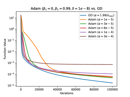
(a) Non-diagonal Hessian

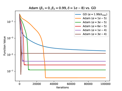
(b) Diagonal Hessian w/ same condition no. as Fig. 1a

Figure 1: In 1a, the Hessian is the first realization of $\bm{Q}$ in Table 2. In 1b, the Hessian is the diagonal matrix containing the eigenvalues of the first realization of $\bm{Q}$ in Table 2. We compare the standard version of Adam in eq. 25 with different step-sizes $\alpha$ against GD with step-size $\alpha={1.99}/{\lambda_{\text{max}}(\bm{Q})}$. Consistent with our theoretical prediction, GD is better than Adam in 1a, whereas Adam is better than GD in 1b.

4.1 Proof Outline of Theorem 3 and Asymptotic Behavior of Adam

We shall now sketch our proof technique for Theorem 3 (detailed proof in Appendix C), i.e., in the case of a general $\bm{Q}$. The proof techniques of other convergence bounds for Adam (Theorems 2 and 8) are similar. This will also shed some light on the behavior of Adam if we let it run forever.

First, we shall introduce some definitions. To that end, recall that $\bm{D}=\bm{Q}\circ\bm{\text{{I}}}$ and the eigen-decomposition of $\bm{Q}$ is $\bm{U}\bm{\Lambda}\bm{U}^{\top}$; thus, $\bm{g}_{k}=\nabla f(\bm{x}_{k})=\bm{U}\bm{\Lambda}\bm{U}^{\top}(\bm{x}_{k}-\bm{x}_{*})$. Now let:

$$\bar{\bm{g}}_{k}:=\bm{\Lambda}^{1/2}{\bm{U}}^{\top}(\bm{x}_{k}-\bm{x}_{*}).$$ (6)

Note that $f(\bm{x}_{k})=\frac{1}{2}\|\bar{\bm{g}}_{k}\|_{2}^{2}$ and $\bm{g}_{k}=\bm{U}\bm{\Lambda}^{1/2}\bar{\bm{g}}_{k}$. Next let:

$$\widehat{\bm{g}}_{k}:=\bm{D}^{-1}\bm{g}_{k}=(\bm{D}^{-1}\bm{U}\bm{\Lambda}^{1/2})\bar{\bm{g}}_{k}=\widehat{\bm{Q}}\bar{\bm{g}}_{k}.$$ (7)

Also, recall that $\bar{\bm{Q}}=\bm{D}^{-1/2}\bm{U}\bm{\Lambda}^{1/2}$. Let:

$$\sigma_{\text{min}}(\bar{\bm{Q}})=\sqrt{\mu_{1}}\text{ and }\sigma_{\text{max}}(\bar{\bm{Q}})=\sqrt{\mu_{2}}.$$ (8)

Since $\text{cond}(\bar{\bm{Q}})=\sqrt{\overline{\kappa}}$, we have $\overline{\kappa}=\big{(}\frac{\mu_{2}}{\mu_{1}}\big{)}$.
Adam’s update rule in eq. 4 with $\beta_{1}=0$ is $x^{(i)}_{k+1}=x^{(i)}_{k}-\frac{\alpha{g}_{k}^{(i)}}{\sqrt{{v}_{k}^{(i)}+\max(({g}_{0}^{(i)})^{2},\phi^{2})\delta_{k}^{2}}}$. Unfolding the recursion of ${v}_{k}^{(i)}$ in eq. 2, we get ${v}_{k}^{(i)}={\sum_{l=0}^{k}\beta_{2}^{k-l}\big{(}{g}_{l}^{(i)}\big{)}^{2}}$. Let ${\bm{V}}_{k}$ be a diagonal matrix whose $i^{\text{th}}$ diagonal element is $\frac{1}{\sqrt{{v}_{k}^{(i)}+\max(({g}_{0}^{(i)})^{2},\phi^{2})\delta_{k}^{2}}}$. Then, we can rewrite Adam’s update rule in matrix-vector notation as:

$$\bm{x}_{k+1}=\bm{x}_{k}-\alpha{\bm{V}}_{k}{\bm{U}}\bm{\Lambda}{\bm{U}}^{\top}(\bm{x}_{k}-\bm{x}_{*}).$$ (9)

After manipulating eq. 9 a bit, we obtain the following equivalent equation:

$$\bar{\bm{g}}_{k+1}=\Big{(}\bm{\text{I}}-\alpha\bm{\Lambda}^{1/2}\bm{U}^{\top}{\bm{V}}_{k}{\bm{U}}\bm{\Lambda}^{1/2}\Big{)}\bar{\bm{g}}_{k},$$ (10)

where $\bar{\bm{g}}_{k}=\bm{\Lambda}^{1/2}{\bm{U}}^{\top}(\bm{x}_{k}-\bm{x}_{*})$ is as defined in eq. 6. From eq. 7, recall that $\widehat{\bm{g}}_{k}=\bm{D}^{-1}\bm{g}_{k}$. Let:

$$\widehat{v}_{k}^{(i)}:={\sum_{l=0}^{k}\beta_{2}^{k-l}\big{(}\widehat{g}_{l}^{(i)}\big{)}^{2}}={\sum_{l=0}^{k}\beta_{2}^{k-l}\big{(}{{g}_{l}^{(i)}}/{q_{i}}\big{)}^{2}}={{v}_{k}^{(i)}}/{q_{i}^{2}}\text{ and }\phi_{i}:={\phi}/{q_{i}}.$$ (11)

Let $\widehat{\bm{V}}_{k}$ be a diagonal matrix whose $i^{\text{th}}$ diagonal element is $\frac{1}{\sqrt{\widehat{v}_{k}^{(i)}+\max((\widehat{g}_{0}^{(i)})^{2},{\phi_{i}^{2}})\delta_{k}^{2}}}$; note that ${\bm{V}}_{k}=\bm{D}^{-1/2}\widehat{\bm{V}}_{k}\bm{D}^{-1/2}$. Plugging this into eq. 10 and recalling that $\bar{\bm{Q}}=\bm{D}^{-1/2}\bm{U}\bm{\Lambda}^{1/2}$, we get:

$$\bar{\bm{g}}_{k+1}={\Big{(}\bm{\text{I}}-\alpha\bar{\bm{Q}}^{\top}\widehat{\bm{V}}_{k}\bar{\bm{Q}}\Big{)}}\bar{\bm{g}}_{k}.$$ (12)

Since $\widehat{\bm{V}}_{k}$ is a diagonal matrix with positive diagonal elements, $\bar{\bm{Q}}^{\top}\widehat{\bm{V}}_{k}\bar{\bm{Q}}$ is symmetric positive-definite (PD). Let $\bm{A}_{k}=\bm{\text{I}}-\alpha\bm{B}_{k}$, where $\bm{B}_{k}=\bar{\bm{Q}}^{\top}\widehat{\bm{V}}_{k}\bar{\bm{Q}}$.

Remark 6 (Basis change).

The basis change in going from eq. 9 to eq. 10 has been chosen to ensure that $\bm{A}_{k}$ is of the form $\bm{\text{I}}-\alpha\bm{B}_{k}$, where $\bm{B}_{k}$ is symmetric PD; in eq. 12, $\bm{B}_{k}=\bar{\bm{Q}}^{\top}\widehat{\bm{V}}_{k}\bar{\bm{Q}}$. If $\bm{B}_{k}$ is not symmetric PD, then the subsequent analysis does not hold. In particular, we cannot directly start the subsequent analysis from eq. 9 (after subtracting $\bm{x}_{*}$ from both sides) because in this case $\bm{B}_{k}$ would be ${\bm{V}}_{k}{\bm{U}}\bm{\Lambda}{\bm{U}}^{\top}$ which is not symmetric unless $\bm{U}=\bm{\text{{I}}}$, i.e., $\bm{Q}=\bm{\Lambda}$ is diagonal.

Remark 7 (Pseudo-linear system).

For a moment, if we ignore the fact that $\bm{A}_{k}$ depends on the iteration number $k$, then eq. 12 is a linear system that we can analyze using standard ideas from linear algebra. Our proof strategy is to treat eq. 12 like a “pseudo-linear” system and involves tracking the evolution of $\bm{A}_{k}$ so that we can utilize standard linear algebra ideas, even though eq. 12 is not truly linear.

Remark 8 (Rationale of going from eq. 10 to eq. 12).

The subsequent steps in the analysis require us to bound $\sigma_{\textup{min}}(\bm{B}_{k})$ and $\sigma_{\textup{max}}(\bm{B}_{k})$ for each $k$. Eq. (10) is equivalent to eq. 12, but the latter can enable us to obtain tighter bounds for $\sigma_{\textup{min}}(\bm{B}_{k})$ and $\sigma_{\textup{max}}(\bm{B}_{k})$ by allowing us to theoretically “cancel out” the dependence on $\kappa$ to an extent (albeit introducing other quantities) – which improves the iteration complexity. Specifically, with eq. 10, we could not improve the $\mathcal{O}(\kappa)$ dependence. But with eq. 12, we get an $\mathcal{O}(\sqrt{\kappa})$ factor in the end for diagonally dominant $\bm{Q}$.

Let $\widehat{w}_{k}^{(j)}=\widehat{v}_{k}^{(j)}+\max((\widehat{g}_{0}^{(j)})^{2},\phi_{j}^{2})\delta_{k}^{2}$. Recalling that $\sigma_{\text{min}}(\bar{\bm{Q}})=\sqrt{\mu_{1}}$ and $\sigma_{\text{max}}(\bar{\bm{Q}})=\sqrt{\mu_{2}}$, we have $\sigma_{\text{max}}(\bar{\bm{Q}}^{\top}\widehat{\bm{V}}_{k}\bar{\bm{Q}})\leq\frac{\mu_{2}}{\sqrt{\min_{j\in[d]}\widehat{w}_{k}^{(j)}}}$ and $\sigma_{\text{min}}(\bar{\bm{Q}}^{\top}\widehat{\bm{V}}_{k}\bar{\bm{Q}})\geq\frac{\mu_{1}}{\sqrt{\max_{j\in[d]}\widehat{w}_{k}^{(j)}}}$. Now at least until ${\min_{j\in[d]}\widehat{w}_{k}^{(j)}}\geq(\mu_{2}\alpha)^{2}$ starting from the first iteration, $\bm{A}_{k}$ is positive semi-definite and we have:

$$\sigma_{\text{max}}(\bm{A}_{k})\leq 1-\frac{\mu_{1}\alpha}{\sqrt{\max_{j\in[d]}\widehat{w}_{k}^{(j)}}}.$$ (13)

So at least until ${\min_{j\in[d]}\widehat{w}_{k}^{(j)}}\geq(\mu_{2}\alpha)^{2}$ holds, descent is ensured in each iteration or there is “continuous descent” and we have:

$$\|\bar{\bm{g}}_{k+1}\|_{2} \leq\sigma_{\text{max}}(\bm{A}_{k})\|\bar{\bm{g}}_{k}\|_{2}\leq\Bigg{(}1-\frac{\mu_{1}\alpha}{\sqrt{\max_{j\in[d]}\widehat{w}_{k}^{(j)}}}\Bigg{)}\|\bar{\bm{g}}_{k}\|_{2}.$$ (14)

In Lemma 2, we analyze the decay rule of eq. 14 until there is continuous descent; suppose this happens for $\tilde{K}$ iterations. Below we present an abridged version of Lemma 2.

Lemma 1 (Abridged version of Lemma 2).

Recall $\widehat{\kappa}=\textup{cond}(\widehat{\bm{Q}})$. Choose $\alpha\leq\frac{\max(3\widehat{\kappa}\sqrt{d}B,\phi/q_{\textup{min}})}{\sqrt{2}\mu_{1}}$, $\beta_{2}=1-\frac{\alpha^{2}\mu_{1}^{2}}{8\max(9\widehat{\kappa}^{2}dB^{2},\phi^{2}/q_{\textup{min}}^{2})}$ and $\delta_{k}=\frac{1}{\sqrt{2(1-\beta_{2})}}\beta_{2}^{\frac{k}{2}}$ for $k\geq 0$. Then for any $k\leq\tilde{K}$, we have:

$$\|\bar{\bm{g}}_{k+1}\|_{2}\leq\exp\Big{(}-2\Big{(}\beta_{2}^{-(k+1)/2}-1\Big{)}\Big{)}\|\bar{\bm{g}}_{0}\|_{2}.$$ (15)

Remark 9 (Proof of Lemma 2).

In Lemma 2, we employ a two-stage analysis procedure wherein we first obtain a loose bound for $\|\bar{\bm{g}}_{k+1}\|_{2}$ in terms of $\|\bar{\bm{g}}_{0}\|_{2}$ (specifically, $\|\bar{\bm{g}}_{k}\|_{2}^{2}\leq\gamma^{k}\|\bar{\bm{g}}_{0}\|_{2}^{2}$ with $\gamma\approx\beta_{2}$), and then obtain a tighter bound by using this loose bound.

We will now elaborate on the two stages in Remark 9.
First Stage. Let us define $\widehat{v}_{k}:=\sum_{j\in[d]}\widehat{v}_{k}^{(j)}={\sum_{l=0}^{k}\beta_{2}^{k-l}\|\widehat{\bm{g}}_{l}\|_{2}^{2}}$. With some simple algebra, we obtain the following relaxation of eq. 14 that is more conducive to analysis:

$$\|\bar{\bm{g}}_{k+1}\|_{2}\leq\Bigg{(}1-\frac{\mu_{1}\alpha}{\sqrt{\widehat{v}_{k}+\max\big{(}\|\widehat{\bm{g}}_{0}\|_{\infty}^{2},\phi^{2}/q_{\text{min}}^{2}){\delta}_{k}^{2}}}\Bigg{)}\|\bar{\bm{g}}_{k}\|_{2}.$$ (16)

From eq. 16, we have $\|\bar{\bm{g}}_{0}\|_{2}\geq\|\bar{\bm{g}}_{1}\|_{2}\geq\ldots\geq\|\bar{\bm{g}}_{\tilde{K}+1}\|_{2}$. Using this with some simple linear algebra, we obtain the following crude bound: $\widehat{v}_{k}\leq\frac{\widehat{\kappa}^{2}\|\widehat{\bm{g}}_{0}\|_{2}^{2}}{1-\beta_{2}}$ $\forall$ $k\leq\tilde{K}+1$. Combining this with our choice of $\delta_{k}$ and using 1, we get:

$$\widehat{v}_{k}+\max\big{(}\|\widehat{\bm{g}}_{0}\|_{\infty}^{2},\phi^{2}/q_{\text{min}}^{2}){\delta}_{k}^{2}\leq\frac{2\max\big{(}9\widehat{\kappa}^{2}dB^{2},\phi^{2}/q_{\text{min}}^{2})}{1-\beta_{2}}.$$ (17)

Note that the above bound is independent of $k$. Plugging this into eq. 16 yields $\|\bar{\bm{g}}_{k+1}\|_{2}^{2}\leq\gamma\|\bar{\bm{g}}_{k}\|_{2}^{2}$, where $\gamma:=\Big{(}1-\frac{{\alpha}\mu_{1}\sqrt{1-\beta_{2}}}{\sqrt{2}\max(3\widehat{\kappa}\sqrt{d}B,\phi/q_{\text{min}})}\Big{)}$. Unfolding this recursion yields:

$$\|\bar{\bm{g}}_{k+1}\|_{2}^{2}\leq\gamma^{k+1}\|\bar{\bm{g}}_{0}\|_{2}^{2}.$$ (18)

The above bound is loose but we will obtain a tighter bound using this bound in the next stage.
Second Stage. With our choice of $\beta_{2}$, we get $\gamma=1-\frac{\alpha^{2}\mu_{1}^{2}}{4\max(9\widehat{\kappa}^{2}dB^{2},\phi^{2}/q_{\text{min}}^{2})}$ and $\beta_{2}-\gamma={1-\beta_{2}}$. Using eq. 18 and with some linear algebra, we get $\|\widehat{\bm{g}}_{l}\|_{2}^{2}\leq\gamma^{l}\widehat{\kappa}^{2}\|\widehat{\bm{g}}_{0}\|_{2}^{2}$. Thus,

$$\widehat{v}_{k}=\sum_{l=0}^{k}\beta_{2}^{k-l}\|\widehat{\bm{g}}_{l}\|_{2}^{2}\leq\sum_{l=0}^{k}\beta_{2}^{k-l}\gamma^{l}\widehat{\kappa}^{2}\|\widehat{\bm{g}}_{0}\|_{2}^{2}=\Bigg{(}\frac{\beta_{2}^{k+1}-\gamma^{k+1}}{\beta_{2}-\gamma}\Bigg{)}\widehat{\kappa}^{2}\|\widehat{\bm{g}}_{0}\|_{2}^{2}\leq\Big{(}\frac{\beta_{2}^{k+1}}{1-\beta_{2}}\Big{)}\widehat{\kappa}^{2}\|\widehat{\bm{g}}_{0}\|_{2}^{2}.$$

Combining this with our choice of $\delta_{k}$ (which was specifically chosen to enable this) and using 1, we get:

$$\widehat{v}_{k}+\max\big{(}\|\widehat{\bm{g}}_{0}\|_{\infty}^{2},\phi^{2}/q_{\text{min}}^{2}){\delta}_{k}^{2}\leq\Big{(}\frac{2\beta_{2}^{k+1}}{1-\beta_{2}}\Big{)}\max\big{(}9\widehat{\kappa}^{2}dB^{2},\phi^{2}/q_{\text{min}}^{2}\big{)}.$$ (19)

Plugging this into eq. 16 (after using the fact that $\exp(-z)\geq 1-z$ $\forall$ $z\in\mathbb{R}$), we get:

$$\|\bar{\bm{g}}_{k+1}\|_{2}\leq\exp\Bigg{(}-\frac{\alpha\mu_{1}\sqrt{1-\beta_{2}}\beta_{2}^{-{(k+1)/2}}}{\sqrt{2}\max\big{(}3\widehat{\kappa}\sqrt{d}B,\phi/q_{\text{min}}\big{)}}\Bigg{)}\|\bar{\bm{g}}_{k}\|_{2}.$$ (20)

Equation 20 is our final per-iteration decay rule of interest. Finally, with some more algebra and simplification, we get the result of Lemma 1 (i.e., eq. 15).
Let us come back to the proof of Theorem 3. From eq. 15, in order to have $\|\bar{\bm{g}}_{K^{*}}\|_{2}\leq\varepsilon$ (and thus, $f(\bm{x}_{{K}^{*}})\leq\frac{\varepsilon^{2}}{2}$), we can choose:

$$K^{*}=\mathcal{O}\Big{(}{\log\Big{(}\log^{2}\Big{(}\frac{\|\bar{\bm{g}}_{0}\|_{2}}{\varepsilon}\Big{)}\Big{)}}\Big{/}{\log\big{(}{1}/{\beta_{2}}\big{)}}\Big{)}.$$ (21)

For the above result to be valid, we must have $K^{*}\leq\tilde{K}$. In Lemma 3, we obtain the following bound for $\tilde{K}$:

$$\tilde{K}={\log\Bigg{(}\frac{\min_{j\in[d]}(\widehat{g}_{0}^{(j)})^{2}}{(\mu_{2}\alpha)^{2}}+\frac{\max(\min_{j\in[d]}(\widehat{g}_{0}^{(j)})^{2},{\phi^{2}}/{q_{\textup{max}}^{2}})}{{2(1-\beta_{2})(\mu_{2}\alpha)^{2}}}\Bigg{)}}\Bigg{/}{\log\big{(}{1}/{\beta_{2}}\big{)}}.$$

We will skip the proof details of Lemma 3 as it is straightforward. Imposing $K^{*}\leq\tilde{K}$ gives us an upper bound for the step-size $\alpha$, viz.,

$$\alpha\leq\mathcal{O}\Bigg{(}\Bigg{(}\frac{\mu_{1}^{2}\max(\min_{j\in[d]}(\widehat{g}_{0}^{(j)})^{2},{\phi^{2}}/{q_{\textup{max}}^{2}})}{\mu_{2}^{2}\max(\widehat{\kappa}^{2}dB^{2},\phi^{2}/q_{\textup{min}}^{2})}\Bigg{)}^{1/4}\frac{\max\big{(}\widehat{\kappa}\sqrt{d}B,\phi/q_{\textup{min}}\big{)}}{\mu_{1}}\log^{-1/2}\Big{(}\frac{\|\bar{\bm{g}}_{0}\|_{2}}{\varepsilon}\Big{)}\Bigg{)}.$$ (22)

From Lemma 4, we have that $\min_{j\in[d]}|\widehat{g}_{0}^{(j)}|>\frac{2B}{d}\Big{(}\frac{\log({1}/{p})}{\zeta\big{(}1+\frac{\log(1/p)}{d}\big{)}}\Big{)}^{1/\theta}$ with a probability of at least $p$. Let $\widetilde{p}=\Big{(}\frac{\log({1}/{p})}{\zeta\big{(}1+\frac{\log(1/p)}{d}\big{)}}\Big{)}^{1/\theta}$. Additionally, we can show that $\|\bar{\bm{g}}_{0}\|_{2}\leq\mathcal{O}(\frac{\sqrt{d}B}{\rho_{1}})$. Thus, with a probability of at least $p$, we can set:

$$\alpha=\mathcal{O}\Bigg{(}\frac{1}{\sqrt{\mu_{1}\mu_{2}}}\Bigg{(}{\max\Big{(}\frac{\widetilde{p}^{2}B^{2}}{d^{2}},\frac{\phi^{2}}{q_{\textup{max}}^{2}}\Big{)}\max\Big{(}\widehat{\kappa}^{2}dB^{2},\frac{\phi^{2}}{q_{\textup{min}}^{2}}\Big{)}}\Bigg{)}^{1/4}\log^{-1/2}\Big{(}\frac{\sqrt{d}B}{\rho_{1}\varepsilon}\Big{)}\Bigg{)}.$$ (23)

Recalling the value of $\beta_{2}$ and using 1, we get $\log\frac{1}{\beta_{2}}\geq\frac{\alpha^{2}\mu_{1}^{2}}{8\max(9\widehat{\kappa}^{2}dB^{2},\phi^{2}/q_{\textup{min}}^{2})}$. Finally, plugging this into eq. 21 with the value of $\alpha$ from eq. 23 and setting $\phi=\widehat{\kappa}\sqrt{d}Bq_{\textup{min}}$ gives us the result of Theorem 3.
An important part of the above analysis is ensuring that we attain $\mathcal{O}({\varepsilon^{2}})$ function value before we can no longer guarantee that $\bm{A}_{k}=\bm{\text{I}}-\alpha\bar{\bm{Q}}^{\top}\widehat{\bm{V}}_{k}\bar{\bm{Q}}$ is positive semi-definite; that is why we impose $K^{*}\leq\tilde{K}$ above and get a constraint on the step-size $\alpha$ (eq. 22). Moreover, we should stop the algorithm at this point because we cannot guarantee continuous descent forever. If there is continuous descent forever, then ${\min_{j\in[d]}\widehat{w}_{k}^{(j)}}$ will also keep decreasing with a decaying $\delta_{k}$ (and a decaying $\delta_{k}$ is required for a “fast decay” rule like eq. 15 to hold). But when ${\min_{j\in[d]}\widehat{w}_{k}^{(j)}}<(\frac{\mu_{2}\alpha}{2})^{2}$, then it may happen that $\lambda_{\text{min}}(\bm{A}_{k})<-1$ and in that case, we can no longer guarantee descent. Therefore, Adam may not enjoy continuous descent forever and it may not converge to zero function value asymptotically. This is consistent with what we observed in Figures 1a and 1b. We formalize this next in Section 4.2.

4.2 Fixed Points of Adam

Here we shall characterize the asymptotic point(s) to which Adam may converge.

Definition 2 (Fixed point).

Consider an iterative and deterministic optimization algorithm $\mathcal{A}$ operating on a function $f(\bm{x})$. Suppose its output at iteration number $k$ is $\bm{x}_{k}$. We define a fixed point of $\mathcal{A}$ to be a point $\overline{\bm{x}}$ such that $\lim_{k\to\infty}f(\bm{x}_{k})=f(\overline{\bm{x}})$.

We have the following result regarding the fixed point(s) $\overline{\bm{x}}$ of Adam for $f(\bm{x})=\frac{1}{2}(\bm{x}-\bm{x}_{*})^{\top}\bm{Q}(\bm{x}-\bm{x}_{*})$ assuming $\lim_{k\to\infty}\delta_{k}$ exists.

Theorem 6 (Fixed point(s) of Adam).

$\overline{\bm{x}}=\bm{x}_{*}$ is a trivial fixed point. There may exist non-trivial fixed points depending on the value of $\lim_{k\to\infty}\delta_{k}=\delta\geq 0$ (note that this also covers the case of the constant sequence $\delta_{k}=\delta$ $\forall$ $k\geq 0$, which is what is used in practice).

• If $\delta=0$, there exists a fixed point $\overline{\bm{x}}\neq\bm{x}_{*}$ with non-zero gradient $\overline{\bm{g}}=\bm{Q}(\overline{\bm{x}}-\bm{x}_{*})$ such that $\|\overline{\bm{g}}\|_{1}\geq\frac{\alpha d\sqrt{1-\beta_{2}}}{2}$.

• If $\delta<\frac{\alpha}{2\overline{R}}$ where $\overline{R}=\max_{j\in[d]}\max(|{g}_{0}^{(j)}|,\phi)$, there exists a fixed point $\overline{\bm{x}}\neq\bm{x}_{*}$ with non-zero gradient $\overline{\bm{g}}=\bm{Q}(\overline{\bm{x}}-\bm{x}_{*})$ such that $\|\overline{\bm{g}}\|_{\infty}\geq\sqrt{(1-\beta_{2})\big{(}\frac{\alpha^{2}}{4}-\overline{R}^{2}\delta^{2}\big{)}}$.

• If $\delta>\frac{\kappa\alpha}{2\overline{r}}$ where $\overline{r}:=\min_{j\in[d]}\max(|{g}_{0}^{(j)}|,\phi)$, $\overline{\bm{x}}=\bm{x}_{*}$ is the only fixed point.

We prove Theorem 6 in Appendix H. For the standard variant of Adam wherein $\max\big{(}({g}_{0}^{(i)})^{2},\phi^{2}\big{)}\delta_{k}^{2}$ is replaced by $\phi^{2}\delta^{2}$ in the denominator of eq. 4, $\overline{R}=\overline{r}=\phi$ in Theorem 6.

Theorem 6 tells us that when $\delta<\frac{\alpha}{2\overline{R}}$, Adam may not converge to the minimum function value $f(\bm{x}_{*})$. When $\delta>\frac{\kappa\alpha}{2\overline{r}}$, Adam will converge to $f(\bm{x}_{*})$. In this case, the effective step-size of Adam in each coordinate is always less than ${2}/{\kappa}$ and so we expect behavior similar to GD, i.e., eventual convergence to the optimum. Unfortunately, we cannot formally assert if there exists a non-trivial fixed point (i.e., $\overline{\bm{x}}\neq\bm{x}_{*}$) when $\delta\in\big{[}\frac{\alpha}{2\overline{R}},\frac{\kappa\alpha}{2\overline{r}}\big{]}$, but we strongly suspect that there are indeed non-trivial fixed points in many cases (as is the case in Figures 1a and 1b).

We will now move on from quadratics and extend our analysis to more general functions.

5 Beyond Quadratics: Per-Coordinate Smoothness and a Modified Polyak-Łojasiewicz (PL) Condition

Here we focus on functions that satisfy per-coordinate Lipschitz smoothness and a modified version of the Polyak-Łojasiewicz (PL) condition. Let us begin by defining the standard global version (with respect to the coordinates) of smoothness and the standard PL condition.

Definition 3 (Smoothness).

$f:\mathbb{R}^{d}\xrightarrow{}\mathbb{R}$ is said to be $L$-smooth if $\forall$ $\bm{x},\bm{y}\in\mathbb{R}^{d}$, it holds that $\|\nabla f(\bm{y})-\nabla f(\bm{x})\|_{2}\leq L\|\bm{y}-\bm{x}\|_{2}$.

Definition 4 (Polyak- Łojasiewicz (PL) Condition (Karimi et al.,, 2016)).

$f:\mathbb{R}^{d}\xrightarrow{}\mathbb{R}$ with $f^{*}:=\min_{\bm{x}\in\mathbb{R}^{d}}f(\bm{x})$ is said to be $\mu$-PL if $\exists$ $\mu>0$ such that:

$$\|\nabla f(\bm{x})\|_{2}^{2}\geq 2\mu(f(\bm{x})-f^{*})\text{ }\forall\text{ }\bm{x}\in\mathbb{R}^{d}.$$

Theorem 7 (GD: Smooth and PL (Karimi et al.,, 2016)).

Suppose $f:\mathbb{R}^{d}\xrightarrow{}\mathbb{R}$ is $L$-smooth and $\mu$-PL, and let $\kappa=\frac{L}{\mu}$ be the condition number. Suppose our initialization is $\bm{x}_{0}$. Set the step-size $\alpha=\frac{1}{L}$. Then, $f(\bm{x}_{\widehat{K}})-f^{*}\leq\varepsilon$ in

$$\widehat{K}=\mathcal{O}\Bigg{(}{\kappa}\log\Bigg{(}\frac{f(\bm{x}_{0})-f^{*}}{\varepsilon}\Bigg{)}\Bigg{)}$$

iterations of GD.

Remark 10.

Similar to the quadratic case (Theorem 1), the iteration complexity of GD depends on the condition number, i.e., $\kappa=\frac{L}{\mu}$.

We will now introduce per-coordinate smoothness and a modified version of the PL condition for functions satisfying per-coordinate smoothness under which we show that Adam can do better than GD.

Definition 5 (Per-Coordinate Smoothness).

$f:\mathbb{R}^{d}\xrightarrow{}\mathbb{R}$ is said to be $\{L_{i}\}_{i=1}^{d}$-smooth if for all $\bm{x},\bm{y}\in\mathbb{R}^{d}$ and for each coordinate $i\in[d]$, it holds that:

$$|\nabla f(\bm{y})^{(i)}-\nabla f(\bm{x})^{(i)}|\leq L_{i}|y^{(i)}-x^{(i)}|.$$

Similar assumptions have been made in the literature (Bernstein et al.,, 2018; Wright,, 2015; Richtárik and Takáč,, 2014).

Definition 6 (Smoothness-Dependent Global PL Condition).

Suppose $f:\mathbb{R}^{d}\xrightarrow{}\mathbb{R}$ is $\{L_{i}\}_{i=1}^{d}$-smooth. Then $f$ is said to obey the smoothness-dependent $\tilde{\mu}$-global-PL condition if $\exists$ $\tilde{\mu}\in(0,\min_{i\in[d]}L_{i}]$ such that:

$$\sum_{i=1}^{d}\frac{(\nabla f(\bm{x})^{(i)})^{2}}{\sqrt{2L_{i}}}\geq\sqrt{2\tilde{\mu}}\big{(}f(\bm{x})-f^{*}\big{)}\text{ }\forall\text{ }\bm{x}\in\mathbb{R}^{d},\text{ where $f^{*}=\min_{\bm{z}\in\mathbb{R}^{d}}f(\bm{z})$.}$$

We are now ready to state our main assumption.

Assumption 2.

$f:\mathbb{R}^{d}\xrightarrow{}\mathbb{R}$ is $\{L_{i}\}_{i=1}^{d}$-smooth and it also satisfies the smoothness-dependent $\tilde{\mu}$-global-PL condition. We are privy to the values of $L_{\textup{min}}:=\min_{i\in[d]}L_{i}$, $L_{\textup{max}}:=\min_{i\in[d]}L_{i}$, $\tilde{\mu}$ and $f^{*}=\min_{\bm{z}\in\mathbb{R}^{d}}f(\bm{z})$.

In many modern machine learning problems, $f^{*}\approx 0$; for e.g., if $f$ is the objective function of an over-parameterized deep network. Also, it can be shown that under 2, $f$ satisfies standard global smoothness (Definition 3) and the standard global PL condition (Definition 4).

Corollary 1.

Suppose 2 holds. Then $f$ is $L_{\textup{max}}$-smooth and $\sqrt{\tilde{\mu}L_{\textup{min}}}$-PL.

For the sake of completeness, we prove Corollary 1 in Appendix J. Based on this and recalling Theorem 7 (and Remark 10), we can make the following remark.

Remark 11.

Under 2, the iteration complexity of GD scales as $\frac{L_{\textup{max}}}{\sqrt{\tilde{\mu}L_{\textup{min}}}}$.

Coming back to Adam, we need one more assumption at the initialization before we can state our result.

Assumption 3 (Per-Coordinate PL-like Condition at Initialization).

At our initialization $\bm{x}_{0}$, the following holds:

$${(\nabla f(\bm{x}_{0})^{(i)})^{2}}\geq 2\mu_{i,0}\big{(}f(\bm{x}_{0})-f^{*}\big{)}$$

for some $\mu_{i,0}\leq L_{i}$ for each $i\in[d]$. Further, the condition number-like quantity $\frac{L_{i}}{\mu_{i,0}}$ along each coordinate $i\in[d]$ at $\bm{x}_{0}$ is bounded, i.e., $\exists$ ${\kappa}_{\textup{max},0}$ such that $\frac{L_{i}}{\mu_{i,0}}\leq{\kappa}_{\textup{max},0}\text{ }\forall\text{ }i\in[d]$. We are privy to the value of ${\kappa}_{\textup{max},0}$.

$\max_{i\in[d]}\frac{L_{i}}{\mu_{i,0}}$ has an implicit dependence on $d$ and so ${\kappa}_{\textup{max},0}$ (which is an upper bound for $\max_{i\in[d]}\frac{L_{i}}{\mu_{i,0}}$) will also have an implicit dependence on $d$. In particular, ${\kappa}_{\textup{max},0}$ should grow with $d$.

Theorem 8 (Adam: Per-Coordinate Smooth and Smoothness-Dependent PL).

Suppose our initialization is $\bm{x}_{0}$ and Assumptions 2 and 3 hold. There exist $\alpha$, $\beta_{2}$, $\delta_{k}$ and $\phi$ such that $f(\bm{x}_{{K}^{*}})-f^{*}\leq\varepsilon$ in

$$K^{*}=\mathcal{O}\Bigg{(}\sqrt{\frac{L_{\textup{max}}}{\tilde{\mu}}}\min\Bigg{(}\sqrt{\frac{L_{\textup{max}}}{L_{\textup{min}}}},\sqrt{{\kappa_{\textup{max},0}}}\Bigg{)}\log\Big{(}\frac{f(\bm{x}_{0})-f^{*}}{\varepsilon}\Big{)}{\log\Big{(}\log\Big{(}\frac{f(\bm{x}_{0})-f^{*}}{\varepsilon}\Big{)}\Big{)}}\Bigg{)}$$

iterations of Adam.

The detailed version and proof of Theorem 8 are in Appendix I.

Remark 12.

The iteration complexity of Adam scales as $\sqrt{\frac{L_{\textup{max}}}{\tilde{\mu}}}\min\Big{(}\sqrt{\frac{L_{\textup{max}}}{L_{\textup{min}}}},\sqrt{{\kappa_{\textup{max},0}}}\Big{)}$. In contrast, the iteration complexity of GD scales as $\frac{L_{\textup{max}}}{\sqrt{\tilde{\mu}L_{\textup{min}}}}=\sqrt{\frac{L_{\textup{max}}}{\tilde{\mu}}}\times\sqrt{\frac{L_{\textup{max}}}{L_{\textup{min}}}}$ per Remark 11. So when $\kappa_{\textup{max},0}<{\frac{L_{\textup{max}}}{L_{\textup{min}}}}$, Adam can outperform GD.

As we discussed after 3, $\kappa_{\textup{max},0}$ should implicitly grow with $d$. Based on this, we can provide the following characterization of when Adam is better than GD in simple words.

Remark 13.

In plain English, Adam can do better than GD when an initialization-dependent quantity which implicitly grows with the dimension is smaller than the ratio of the maximum and minimum per-coordinate smoothness constants.

Appendix

Contents

• Appendix A: Connection of the Update Rule in Eq. 3 to the Vanilla Version of Adam

• Appendix B: Difficulty with Uniform Random Sampling for Non-Diagonal Quadratics

• Appendix C: Detailed Version and Proof of Theorem 3

• Appendix D: Detailed Version and Proof of Theorem 2

• Appendix E: Proof of Theorem 5

• Appendix F: Proof of Theorem 4

• Appendix G: Proof of Proposition 1

• Appendix H: Proof of Theorem 6

• Appendix I: Detailed Version and Proof of Theorem 8

• Appendix J: Proof of Corollary 1

Appendix A Connection of the Update Rule in Eq. 3 to the Vanilla Version of Adam

We will first state the vanilla version of Adam proposed by Kingma and Ba, (2014). For each $i\in\{1,\ldots,d\}$, let:

$$\overline{m}_{k}^{(i)}=\beta_{1}\overline{m}_{k-1}^{(i)}+(1-\beta_{1}){g}_{k}^{(i)}\text{ with }\overline{m}_{0}^{(i)}=0\text{ and }\overline{v}_{k}^{(i)}=\beta_{2}\overline{v}_{k-1}^{(i)}+(1-\beta_{2})\big{(}{g}_{k}^{(i)}\big{)}^{2}\text{ with }\overline{v}_{k}^{(i)}=0,$$ (24)

where recall that $\bm{g}_{k}=\nabla f(\bm{x}_{k})$. The update rule of the $i^{\text{th}}$ coordinate in the $k^{\text{th}}$ iteration of the vanilla version of Adam proposed by (Kingma and Ba,, 2014) is:

$$x^{(i)}_{k+1}=x^{(i)}_{k}-\frac{\alpha\widetilde{m}_{k}^{(i)}}{\sqrt{\widetilde{v}_{k}^{(i)}}+{\delta}},$$ (25)

where $\widetilde{m}_{k}^{(i)}=\frac{\overline{m}_{k}^{(i)}}{1-\beta_{1}^{k+1}}$, $\widetilde{v}_{k}^{(i)}=\frac{\overline{v}_{k}^{(i)}}{1-\beta_{2}^{k+1}}$, $\alpha$ is the step-size, $\beta_{1},\beta_{2}\in(0,1)$ are the first moment/momentum and second moment hyper-parameters, and ${\delta}$ is a correction term in the update’s denominator.

We will now show the relation between eq. 25 and eq. 3. To that end, recall that in eq. 3, we had:

$${m}_{k}^{(i)}=\beta_{1}{m}_{k-1}^{(i)}+{g}_{k}^{(i)}\text{ with }{m}_{0}^{(i)}=0\text{ and }{v}_{k}^{(i)}=\beta_{2}{v}_{k-1}^{(i)}+\big{(}{g}_{k}^{(i)}\big{)}^{2}\text{ with }{v}_{0}^{(i)}=0.$$ (26)

It can be verified that $\overline{m}_{k}^{(i)}=(1-\beta_{1}){m}_{k}^{(i)}$ and $\overline{v}_{k}^{(i)}=(1-\beta_{2}){v}_{k}^{(i)}$. Thus,

$$\widetilde{m}_{k}^{(i)}={{m}_{k}^{(i)}}\Big{/}{\Big{(}\frac{1-\beta_{1}^{k+1}}{1-\beta_{1}}\Big{)}}\text{ and }\widetilde{v}_{k}^{(i)}={{v}_{k}^{(i)}}\Big{/}{\Big{(}\frac{1-\beta_{2}^{k+1}}{1-\beta_{2}}\Big{)}}.$$

Plugging this into eq. 25, we get:

$$x^{(i)}_{k+1}=x^{(i)}_{k}-\Bigg{(}\alpha\Bigg{(}\frac{1-\beta_{1}}{\sqrt{1-\beta_{2}}}\Bigg{)}\Bigg{(}\frac{\sqrt{1-\beta_{2}^{k+1}}}{1-\beta_{1}^{k+1}}\Bigg{)}\Bigg{)}\frac{{m}_{k}^{(i)}}{\sqrt{{v}_{k}^{(i)}}+{\delta}\sqrt{\frac{{1-\beta_{2}^{k+1}}}{1-\beta_{2}}}},$$ (27)

We disregard the “bias-correction” terms $(1-\beta_{1}^{k+1})$ and $(1-\beta_{2}^{k+1})$ because they do not yield any theoretical improvement and converge to $1$. With that, eq. 27 becomes:

$$x^{(i)}_{k+1}=x^{(i)}_{k}-\alpha\Bigg{(}\frac{1-\beta_{1}}{\sqrt{1-\beta_{2}}}\Bigg{)}\frac{{m}_{k}^{(i)}}{\sqrt{{v}_{k}^{(i)}}+{\frac{{\delta}}{\sqrt{1-\beta_{2}}}}}.$$ (28)

Pushing the $\frac{{\delta}}{\sqrt{1-\beta_{2}}}$ term inside the $\sqrt{{v}_{k}^{(i)}}$ term does not really change anything meaningfully; that gives us:

$$x^{(i)}_{k+1}=x^{(i)}_{k}-\alpha\Bigg{(}\frac{1-\beta_{1}}{\sqrt{1-\beta_{2}}}\Bigg{)}\frac{{m}_{k}^{(i)}}{\sqrt{{v}_{k}^{(i)}+\frac{{\delta}^{2}}{1-\beta_{2}}}}.$$ (29)

Note that eq. 3 is equivalent to eq. 29; specifically, $\alpha$ and $\delta$ of eq. 3 correspond to $\alpha\Big{(}\frac{1-\beta_{1}}{\sqrt{1-\beta_{2}}}\Big{)}$ and $\frac{{\delta}^{2}}{1-\beta_{2}}$ of eq. 29, respectively.

Appendix B Difficulty with Uniform Random Sampling for Non-Diagonal Quadratics

Here we will discuss the difficulty of deriving a result if $\bm{x}_{0}$ is sampled uniformly at random like the diagonal case (Theorem 2). We need a high-probability lower bound for $\min_{i\in[d]}|\widehat{g}_{0}^{(i)}|$, where recall that $\widehat{\bm{g}}_{0}=\bm{T}(\bm{x}_{0}-\bm{x}_{*})$ and $\bm{T}=\bm{D}^{-1}\bm{Q}$. Suppose $\|\bm{x}_{*}\|_{\infty}\leq B$ and ${x}_{0}^{(i)}\underset{\textup{iid}}{\sim}\textup{Unif}[-2B,2B]$ $\forall$ $i\in[d]$. Let $\mathcal{P}(\bm{T}):=\{\bm{y}\text{ }|\text{ }\bm{y}=\bm{T}(\bm{x}-\bm{x}_{*})\text{ s.t. }\|\bm{x}\|_{\infty}\leq 2B\}$. The density function for any $\bm{y}\in\mathcal{P}(\bm{T})$ is given by $p(\bm{y})=\frac{1}{(4B)^{d}\text{det}(\bm{T})}$. So:

$$\mathbb{P}\Big{(}\min_{i\in[d]}|\widehat{g}_{0}^{(i)}|>w\Big{)}=\frac{1}{(4B)^{d}\text{det}(\bm{T})}\int_{\bm{y}\in\mathcal{P}(\bm{T})}\Pi_{i\in[d]}\mathds{1}\Big{(}|y^{(i)}|\geq w\Big{)}\bm{dy}.$$ (30)

The above volumetric integral seems hard to evaluate in general. This is the main difficulty in deriving a result if $\bm{x}_{0}$ is sampled uniformly at random. However, we can indeed get a result if $\bm{Q}$ is close to diagonal and we discuss this next.

B.1 Approximately Diagonal Case

Note that $\widehat{\bm{g}}_{0}=(\bm{x}_{0}-\bm{x}_{*})+\big{(}\bm{T}-\bm{\text{{I}}}\big{)}(\bm{x}_{0}-\bm{x}_{*})$. Let $\bm{z}_{0}=\bm{x}_{0}-\bm{x}_{*}$ and $\bm{T}^{\prime}=\bm{T}-\bm{\text{{I}}}$. Since $\bm{T}=\bm{D}^{-1}\bm{Q}$, we have that $T^{\prime}[i,j]=\frac{Q[i,j]}{q_{i}}$ for $j\neq i$ and $T^{\prime}[i,i]=0$. Let $\nu=\max_{i\in[d]}\sum_{j\neq i}T^{\prime}[i,j]$. When $\nu$ is small enough:

$$|\widehat{{g}}_{0}^{(i)}|\geq|z_{0}^{(i)}|-\nu\|\bm{z}_{0}\|_{\infty}\text{ }\forall\text{ }i\in[d].$$ (31)

Since $\|\bm{x}_{0}\|_{\infty}\leq 2B$ and $\|\bm{x}_{*}\|_{\infty}\leq B$, we have $\|\bm{z}_{0}\|_{\infty}\leq 3B$. Using this above, we get:

$$|\widehat{{g}}_{0}^{(i)}|\geq|z_{0}^{(i)}|-\nu(3B)\text{ }\forall\text{ }i\in[d].$$ (32)

From Lemma 7, we have that $\min_{i\in[d]}|{z}_{0}^{(i)}|>\Big{(}\frac{2\log({1}/{p})}{1+\frac{\log({1}/{p})}{d}}\Big{)}\frac{B}{d}$ with a probability of at least $p$. So when $\nu\leq\frac{1}{3d}$:

$$\min_{i\in[d]}|\widehat{{g}}_{0}^{(i)}|>\Bigg{(}\frac{2\log({1}/{p})}{1+\frac{\log({1}/{p})}{d}}-1\Bigg{)}\frac{B}{d},$$

with a probability of at least $p$. We can use the bound above to obtain a result similar to Theorem 3 (with $\theta=1$).

Appendix C Detailed Version and Proof of Theorem 3

We need to introduce a couple of quantities first. Recall that $\bar{\bm{Q}}=\bm{D}^{-1/2}\bm{U}\bm{\Lambda}^{1/2}$. Let:

$$\sigma_{\text{min}}(\bar{\bm{Q}})=\sqrt{\mu_{1}}\text{ and }\sigma_{\text{max}}(\bar{\bm{Q}})=\sqrt{\mu_{2}}.$$ (33)

Since $\text{cond}(\bar{\bm{Q}})=\sqrt{\overline{\kappa}}$, we have $\overline{\kappa}=\big{(}\frac{\mu_{2}}{\mu_{1}}\big{)}$. We are now ready to state the detailed version of Theorem 3.

Theorem 9 (Detailed Version of Theorem 3).

Suppose our initialization $\bm{x}_{0}$ satisfies 1. Fix some $p\in[\frac{1}{e},1)$. Choose

$$\alpha=\mathcal{O}\Bigg{(}\frac{\widehat{\kappa}\sqrt{d}B}{\sqrt{\mu_{1}\mu_{2}}}\Big{(}{\max\Big{(}\frac{\widetilde{p}^{2}}{\widehat{\kappa}^{2}d^{3}},\frac{1}{\kappa_{\textup{diag}}^{2}}\Big{)}}\Big{)}^{1/4}\log^{-1/2}\Big{(}\frac{\sqrt{d}B}{\rho_{1}\varepsilon}\Big{)}\Bigg{)}\text{ where }\widetilde{p}=\Bigg{(}\frac{\log({1}/{p})}{\zeta\big{(}1+\frac{\log(1/p)}{d}\big{)}}\Bigg{)}^{1/\theta},$$

$$\beta_{2}=1-\frac{\alpha^{2}\mu_{1}^{2}}{72\widehat{\kappa}^{2}dB^{2}},\text{ }\delta_{k}=\frac{\beta_{2}^{{k}/{2}}}{\sqrt{2(1-\beta_{2})}}\text{ and }\phi=\widehat{\kappa}\sqrt{d}Bq_{\textup{min}}.$$

Then with a probability of at least $p$ over the randomness of $\bm{x}_{0}$, $f(\bm{x}_{{K}^{*}})<\frac{\varepsilon^{2}}{2}$ in

$$K^{*}=\mathcal{O}\Bigg{(}\kappa_{\textup{Adam}}\log\Big{(}\frac{\sqrt{d}B}{\rho_{1}\varepsilon}\Big{)}{\log\Big{(}\log\Big{(}\frac{\|\bm{\Lambda}^{1/2}{\bm{U}}^{\top}(\bm{x}_{0}-\bm{x}_{*})\|_{2}}{\varepsilon}\Big{)}\Big{)}}\Bigg{)}$$

iterations of Adam, where $\kappa_{\textup{Adam}}:=\overline{\kappa}\min\Big{(}\Big{(}\frac{\widehat{\kappa}d^{3/2}}{\log^{1/\theta}({1}/{p})}\Big{)}\zeta^{1/\theta}\big{(}1+\frac{\log(1/p)}{d}\big{)}^{1/\theta},\kappa_{\textup{diag}}\Big{)}$.

For setting the hyper-parameters listed above, we need to be privy to $\mu_{1}$, $\mu_{2}$, $\rho_{1}$, $\rho_{2}$ (recall $\widehat{\kappa}=\frac{\rho_{2}}{\rho_{1}}$), $q_{\textup{max}}$ and $q_{\textup{min}}$ (recall $\kappa_{\textup{diag}}=\frac{q_{\textup{max}}}{q_{\textup{min}}}$). It is true that we require more knowledge about the problem compared to GD, but we would like to emphasize that the main point of the results in this paper is to quantify how well Adam can do with a bit more information about the problem. In this sense, our results are a significant departure from most prior results that do not quantify the gains of Adam over GD in terms of dependence on the condition number of the Hessian. Moreover, the dependence of GD cannot be improved even if we are privy to these quantities.

Proof.

Adam’s update rule in eq. 4 with $\beta_{1}=0$ becomes:

$$x^{(i)}_{k+1}=x^{(i)}_{k}-\frac{\alpha{g}_{k}^{(i)}}{\sqrt{{v}_{k}^{(i)}+\max\Big{(}\big{(}{g}_{0}^{(i)}\big{)}^{2},\phi^{2}\Big{)}\delta_{k}^{2}}},$$ (34)

where ${v}_{k}^{(i)}:={\sum_{l=0}^{k}\beta_{2}^{k-l}\big{(}{g}_{l}^{(i)}\big{)}^{2}}$ and ${g}_{k}^{(i)}$ is the $i^{\text{th}}$ coordinate of $\bm{g}_{k}=\nabla f(\bm{x}_{k})=\bm{Q}(\bm{x}_{k}-\bm{x}_{*})$. Let ${\bm{V}}_{k}$ be a diagonal matrix whose $i^{\text{th}}$ diagonal element is $\frac{1}{\sqrt{{v}_{k}^{(i)}+\max(({g}_{0}^{(i)})^{2},\phi^{2})\delta_{k}^{2}}}$. Then, we can rewrite eq. 34 in matrix-vector notation as:

$$\bm{x}_{k+1}=\bm{x}_{k}-\alpha{\bm{V}}_{k}{\bm{g}}_{k}=\bm{x}_{k}-\alpha{\bm{V}}_{k}{\bm{Q}}(\bm{x}_{k}-\bm{x}_{*})=\bm{x}_{k}-\alpha{\bm{V}}_{k}{\bm{U}}\bm{\Lambda}{\bm{U}}^{\top}(\bm{x}_{k}-\bm{x}_{*}).$$ (35)

Subtracting $\bm{x}_{*}$ from both sides above and then pre-multiplying by $\bm{\Lambda}^{1/2}\bm{U}^{\top}$ on both sides, we get:

$$\bm{\Lambda}^{1/2}\bm{U}^{\top}(\bm{x}_{k+1}-\bm{x}_{*})=\bm{\Lambda}^{1/2}\bm{U}^{\top}(\bm{x}_{k}-\bm{x}_{*})-\alpha\big{(}\bm{\Lambda}^{1/2}\bm{U}^{\top}{\bm{V}}_{k}{\bm{U}}\bm{\Lambda}^{1/2}\big{)}\bm{\Lambda}^{1/2}{\bm{U}}^{\top}(\bm{x}_{k}-\bm{x}_{*}).$$ (36)

Let us define $\bar{\bm{g}}_{k}:=\bm{\Lambda}^{1/2}{\bm{U}}^{\top}(\bm{x}_{k}-\bm{x}_{*})$; note that $\bm{g}_{k}=\bm{U}\bm{\Lambda}^{1/2}\bar{\bm{g}}_{k}$. Then we can re-write the above equation as:

$$\bar{\bm{g}}_{k+1}=\Big{(}\bm{\text{I}}-\alpha\bm{\Lambda}^{1/2}\bm{U}^{\top}{\bm{V}}_{k}{\bm{U}}\bm{\Lambda}^{1/2}\Big{)}\bar{\bm{g}}_{k}.$$ (37)

Let us also define $\widehat{\bm{g}}_{k}:=\bm{D}^{-1}\bm{g}_{k}=(\bm{D}^{-1}\bm{U}\bm{\Lambda}^{1/2})\bar{\bm{g}}_{k}=\widehat{\bm{Q}}\bar{\bm{g}}_{k}$. Note that the $i^{\text{th}}$ coordinate of $\widehat{\bm{g}}_{k}$ denoted by $\widehat{{g}}_{k}^{(i)}$ is simply $\frac{{g}_{k}^{(i)}}{{q_{i}}}$, where recall that $q_{i}=Q[i,i]$. Let

$$\widehat{v}_{k}^{(i)}:={\sum_{l=0}^{k}\beta_{2}^{k-l}\big{(}\widehat{g}_{l}^{(i)}\big{)}^{2}}=\frac{{v}_{k}^{(i)}}{q_{i}^{2}}.$$ (38)

Also define $\widehat{\bm{V}}_{k}$ to be a diagonal matrix whose $i^{\text{th}}$ diagonal element is $\frac{1}{\sqrt{\widehat{v}_{k}^{(i)}+\max((\widehat{g}_{0}^{(i)})^{2},{\phi_{i}^{2}})\delta_{k}^{2}}}$, where $\phi_{i}:=\frac{\phi}{q_{i}}$. Note that ${\bm{V}}_{k}=\bm{D}^{-1/2}\widehat{\bm{V}}_{k}\bm{D}^{-1/2}$. Plugging this into eq. 37, we get:

$$\bar{\bm{g}}_{k+1}=\Big{(}\bm{\text{I}}-\alpha\bm{\Lambda}^{1/2}\bm{U}^{\top}\bm{D}^{-1/2}\widehat{\bm{V}}_{k}\bm{D}^{-1/2}{\bm{U}}\bm{\Lambda}^{1/2}\Big{)}\bar{\bm{g}}_{k}.$$ (39)

Recalling that $\bar{\bm{Q}}=\bm{D}^{-1/2}\bm{U}\bm{\Lambda}^{1/2}$, we can rewrite the above equation as:

$$\bar{\bm{g}}_{k+1}=\underbrace{\Big{(}\bm{\text{I}}-\alpha\bar{\bm{Q}}^{\top}\widehat{\bm{V}}_{k}\bar{\bm{Q}}\Big{)}}_{:=\bm{A}_{k}}\bar{\bm{g}}_{k}.$$ (40)

Since $\widehat{\bm{V}}_{k}$ is a diagonal matrix with positive diagonal elements, $\bar{\bm{Q}}^{\top}\widehat{\bm{V}}_{k}\bar{\bm{Q}}$ is symmetric positive-definite (PD). Recall that $\sigma_{\text{min}}(\bar{\bm{Q}})=\sigma_{\text{min}}(\bar{\bm{Q}}^{\top})=\sqrt{\mu_{1}}$ and $\sigma_{\text{max}}(\bar{\bm{Q}})=\sigma_{\text{max}}(\bar{\bm{Q}}^{\top})=\sqrt{\mu_{2}}$. Thus, we have that:

$$\sigma_{\text{max}}(\bar{\bm{Q}}^{\top}\widehat{\bm{V}}_{k}\bar{\bm{Q}})\leq\sigma_{\text{max}}(\bar{\bm{Q}}^{\top})\sigma_{\text{max}}(\widehat{\bm{V}}_{k})\sigma_{\text{max}}(\bar{\bm{Q}})\leq\frac{\mu_{2}}{\sqrt{\min_{j\in[d]}\big{(}\widehat{v}_{k}^{(j)}+\max((\widehat{g}_{0}^{(j)})^{2},\phi_{j}^{2})\delta_{k}^{2}\big{)}}}$$

and

$$\sigma_{\text{min}}(\bar{\bm{Q}}^{\top}\widehat{\bm{V}}_{k}\bar{\bm{Q}})\geq\sigma_{\text{min}}(\bar{\bm{Q}}^{\top})\sigma_{\text{min}}(\widehat{\bm{V}}_{k})\sigma_{\text{min}}(\bar{\bm{Q}})\geq\frac{\mu_{1}}{\sqrt{\max_{j\in[d]}\big{(}\widehat{v}_{k}^{(j)}+\max((\widehat{g}_{0}^{(j)})^{2},\phi_{j}^{2})\delta_{k}^{2}\big{)}}}.$$

Now at least until ${\min_{j\in[d]}\big{(}\widehat{v}_{k}^{(j)}+\max\big{(}(\widehat{g}_{0}^{(j)})^{2},\phi_{j}^{2}\big{)}\delta_{k}^{2}\big{)}}\geq(\mu_{2}\alpha)^{2}$ starting from the first iteration, $\bm{A}_{k}=\bm{\text{I}}-\alpha\bar{\bm{Q}}^{\top}\widehat{\bm{V}}_{k}\bar{\bm{Q}}$ is positive semi-definite and we have:

$$\sigma_{\text{max}}(\bm{A}_{k})\leq 1-\frac{\mu_{1}\alpha}{\sqrt{\max_{j\in[d]}\big{(}\widehat{v}_{k}^{(j)}+\max\big{(}(\widehat{g}_{0}^{(j)})^{2},\phi_{j}^{2}\big{)}\delta_{k}^{2}\big{)}}}.$$ (41)

So at least until ${\min_{j\in[d]}\big{(}\widehat{v}_{k}^{(j)}+\max\big{(}(\widehat{g}_{0}^{(j)})^{2},\phi_{j}^{2}\big{)}\delta_{k}^{2}\big{)}}\geq(\mu_{2}\alpha)^{2}$ holds, descent is ensured in each iteration or there is “continuous descent” and we have:

$$\|\bar{\bm{g}}_{k+1}\|_{2} \leq\sigma_{\text{max}}(\bm{A}_{k})\|\bar{\bm{g}}_{k}\|_{2}$$

$$\leq\Bigg{(}1-\frac{\mu_{1}\alpha}{\sqrt{\max_{j\in[d]}\big{(}\widehat{v}_{k}^{(j)}+\max\big{(}(\widehat{g}_{0}^{(j)})^{2},\phi_{j}^{2}\big{)}\delta_{k}^{2}\big{)}}}\Bigg{)}\|\bar{\bm{g}}_{k}\|_{2}.$$ (42)

Suppose we have continuous descent until $\tilde{K}$ iterations, i.e.,

$${\min_{j\in[d]}\big{(}\widehat{v}_{k}^{(j)}+\max\big{(}(\widehat{g}_{0}^{(j)})^{2},\phi_{j}^{2}\big{)}\delta_{k}^{2}\big{)}}\geq(\mu_{2}\alpha)^{2}\text{ }\forall\text{ }k\in\{0,\ldots,\tilde{K}\}.$$

Choose $\alpha\leq\frac{\max(3\widehat{\kappa}\sqrt{d}B,\phi/q_{\textup{min}})}{\sqrt{2}\mu_{1}}$, $\beta_{2}=1-\frac{\alpha^{2}\mu_{1}^{2}}{8\max(9\widehat{\kappa}^{2}dB^{2},\phi^{2}/q_{\textup{min}}^{2})}$ and $\delta_{k}=\frac{1}{\sqrt{2(1-\beta_{2})}}\beta_{2}^{\frac{k}{2}}$. From Lemma 3, we have continuous descent until at least

$$\tilde{K} =\frac{\log\Big{(}\frac{\min_{j\in[d]}(\widehat{g}_{0}^{(j)})^{2}}{(\mu_{2}\alpha)^{2}}+\frac{\max(\min_{j\in[d]}(\widehat{g}_{0}^{(j)})^{2},{\phi^{2}}/{q_{\textup{max}}^{2}})}{{2(1-\beta_{2})(\mu_{2}\alpha)^{2}}}\Big{)}}{\log\frac{1}{\beta_{2}}}$$

$$=\frac{\log\Big{(}\frac{\min_{j\in[d]}(\widehat{g}_{0}^{(j)})^{2}}{\mu_{2}^{2}\alpha^{2}}+\frac{4\max(\min_{j\in[d]}(\widehat{g}_{0}^{(j)})^{2},{\phi^{2}}/{q_{\textup{max}}^{2}})\max(9\widehat{\kappa}^{2}dB^{2},\phi^{2}/q_{\textup{min}}^{2})}{\mu_{2}^{2}\mu_{1}^{2}\alpha^{4}}\Big{)}}{\log\frac{1}{\beta_{2}}}$$ (43)

iterations. The last equality in eq. 43 follows by plugging in the value of $\beta_{2}=1-\frac{\alpha^{2}\mu_{1}^{2}}{8\max(9\widehat{\kappa}^{2}dB^{2},\phi^{2}/q_{\textup{min}}^{2})}$. Also from Lemma 2, we have for any $k\in\{1,\ldots,\tilde{K}\}$:

$$\|\bar{\bm{g}}_{k}\|_{2}\leq\exp\Big{(}-2\big{(}\beta_{2}^{-{k}/{2}}-1\big{)}\Big{)}\|\bar{\bm{g}}_{0}\|_{2}.$$ (44)

Now in order to have $\|\bar{\bm{g}}_{K^{*}}\|_{2}\leq\varepsilon$, we can choose:

$$K^{*}=\frac{\log\Big{(}\frac{1}{4}\log^{2}\Big{(}\frac{e^{2}\|\bar{\bm{g}}_{0}\|_{2}}{\varepsilon}\Big{)}\Big{)}}{\log\frac{1}{\beta_{2}}}.$$ (45)

Now in order for this result to be applicable, let us ensure $K^{*}\leq\tilde{K}$; for this, we must have:

$$\frac{1}{4}\log^{2}\Big{(}\frac{e^{2}\|\bar{\bm{g}}_{0}\|_{2}}{\varepsilon}\Big{)}\leq\frac{\min_{j\in[d]}(\widehat{g}_{0}^{(j)})^{2}}{\mu_{2}^{2}\alpha^{2}}+\frac{4\max(\min_{j\in[d]}(\widehat{g}_{0}^{(j)})^{2},{\phi^{2}}/q_{\textup{max}}^{2})\max(9\widehat{\kappa}^{2}dB^{2},\phi^{2}/q_{\textup{min}}^{2})}{\mu_{2}^{2}\mu_{1}^{2}\alpha^{4}}.$$ (46)

The above can be ensured by simply having:

$$\frac{1}{4}\log^{2}\Big{(}\frac{e^{2}\|\bar{\bm{g}}_{0}\|_{2}}{\varepsilon}\Big{)}\leq\frac{4\max(\min_{j\in[d]}(\widehat{g}_{0}^{(j)})^{2},{\phi^{2}}/q_{\textup{max}}^{2})\max(9\widehat{\kappa}^{2}dB^{2},\phi^{2}/q_{\textup{min}}^{2})}{\mu_{2}^{2}\mu_{1}^{2}\alpha^{4}},$$ (47)

and this gives us:

$$\alpha\leq\mathcal{O}\Bigg{(}\Bigg{(}\frac{\mu_{1}^{2}\max(\min_{j\in[d]}(\widehat{g}_{0}^{(j)})^{2},{\phi^{2}}/q_{\textup{max}}^{2})}{\mu_{2}^{2}\max(\widehat{\kappa}^{2}dB^{2},\phi^{2}/q_{\textup{min}}^{2})}\Bigg{)}^{1/4}\frac{\max\big{(}\widehat{\kappa}\sqrt{d}B,\phi/q_{\textup{min}}\big{)}}{\mu_{1}}\log^{-1/2}\Big{(}\frac{\|\bar{\bm{g}}_{0}\|_{2}}{\varepsilon}\Big{)}\Bigg{)}.$$ (48)

Earlier, we had imposed $\alpha\leq\frac{\max(3\widehat{\kappa}\sqrt{d}B,\phi/q_{\textup{min}})}{\sqrt{2}\mu_{1}}$; note that the above constraint satisfies this requirement. This is because $\mu_{1}\leq\mu_{2}$ and $\max(\min_{j\in[d]}(\widehat{g}_{0}^{(j)})^{2},{\phi^{2}}/q_{\textup{max}}^{2})\leq\max(\widehat{\kappa}^{2}d\|\widehat{\bm{g}}_{0}\|_{\infty}^{2},\phi^{2}/q_{\textup{min}}^{2})\leq\mathcal{O}\big{(}\max(\widehat{\kappa}^{2}dB^{2},\phi^{2}/q_{\textup{min}}^{2})\big{)}$, where the last step follows from the fact that $\|\widehat{\bm{g}}_{0}\|_{\infty}\leq 3B$ (from 1). From Lemma 4, we have $\min_{j\in[d]}|\widehat{g}_{0}^{(j)}|>\frac{2B}{d}\Big{(}\frac{\log({1}/{p})}{\zeta\big{(}1+\frac{\log(1/p)}{d}\big{)}}\Big{)}^{1/\theta}$ with a probability of at least $p$. For simplicity of notation, let $\widetilde{p}=\Big{(}\frac{\log({1}/{p})}{\zeta\big{(}1+\frac{\log(1/p)}{d}\big{)}}\Big{)}^{1/\theta}$. Moreover, since $\widehat{\bm{g}}_{0}=\widehat{\bm{Q}}\bar{\bm{g}}_{0}$ and $\sigma_{\text{min}}(\widehat{\bm{Q}})={\rho_{1}}$, $\|\bar{\bm{g}}_{0}\|_{2}\leq\frac{\|\widehat{\bm{g}}_{0}\|_{2}}{\rho_{1}}\leq\frac{\sqrt{d}\|\widehat{\bm{g}}_{0}\|_{\infty}}{\rho_{1}}\leq\mathcal{O}(\frac{\sqrt{d}B}{\rho_{1}})$ (where the last step follows because $\|\widehat{\bm{g}}_{0}\|_{\infty}\leq 3B$). Thus, with a probability of at least $p$, we can pick:

$$\alpha=\mathcal{O}\Bigg{(}\frac{1}{\sqrt{\mu_{1}\mu_{2}}}\Bigg{(}{\max\Bigg{(}\frac{\widetilde{p}^{2}B^{2}}{d^{2}},\frac{\phi^{2}}{q_{\textup{max}}^{2}}\Bigg{)}\max\Bigg{(}\widehat{\kappa}^{2}dB^{2},\frac{\phi^{2}}{q_{\textup{min}}^{2}}\Bigg{)}}\Bigg{)}^{1/4}\log^{-1/2}\Big{(}\frac{\sqrt{d}B}{\rho_{1}\varepsilon}\Big{)}\Bigg{)}.$$ (49)

Next, recalling that $\beta_{2}=1-\frac{\alpha^{2}\mu_{1}^{2}}{8\max(9\widehat{\kappa}^{2}dB^{2},\phi^{2}/q_{\textup{min}}^{2})}$, $\log\frac{1}{\beta_{2}}\geq\frac{\alpha^{2}\mu_{1}^{2}}{8\max(9\widehat{\kappa}^{2}dB^{2},\phi^{2}/q_{\textup{min}}^{2})}$ using 1. Plugging this in the expression of $K^{*}$ (eq. 45), we get:

$$K^{*}=\mathcal{O}\Bigg{(}\frac{\max(\widehat{\kappa}^{2}dB^{2},\phi^{2}/q_{\textup{min}}^{2})}{{\alpha}^{2}\mu_{1}^{2}}{\log\Big{(}\log\Big{(}\frac{\|\bar{\bm{g}}_{0}\|_{2}}{\varepsilon}\Big{)}\Big{)}}\Bigg{)}.$$ (50)

Plugging in the value of $\alpha$ from eq. 49 while recalling that $\overline{\kappa}=\frac{\mu_{2}}{\mu_{1}}$, we get:

$$K^{*}=\mathcal{O}\Bigg{(}\overline{\kappa}\Bigg{(}\frac{\max\big{(}\widehat{\kappa}\sqrt{d}B,\frac{\phi}{q_{\textup{min}}}\big{)}}{\max\big{(}\frac{\widetilde{p}B}{d},\frac{\phi}{q_{\textup{max}}}\big{)}}\Bigg{)}\log\Big{(}\frac{\sqrt{d}B}{\rho_{1}\varepsilon}\Big{)}{\log\Big{(}\log\Big{(}\frac{\|\bar{\bm{g}}_{0}\|_{2}}{\varepsilon}\Big{)}\Big{)}}\Bigg{)},$$ (51)

with a probability of at least $p$ over random initialization. Next, recall that $\bar{\bm{g}}_{{K}^{*}}:=\bm{\Lambda}^{1/2}{\bm{U}}^{\top}(\bm{x}_{{K}^{*}}-\bm{x}_{*})$. Also, we have that:

$$f(\bm{x}_{{K}^{*}})=\frac{1}{2}(\bm{x}_{{K}^{*}}-\bm{x}_{*})^{\top}\bm{Q}(\bm{x}_{{K}^{*}}-\bm{x}_{*})=\frac{1}{2}\|\bar{\bm{g}}_{{K}^{*}}\|_{2}^{2}.$$

So $\|\bar{\bm{g}}_{K^{*}}\|_{2}\leq\varepsilon$ implies $f(\bm{x}_{{K}^{*}})\leq\frac{\varepsilon^{2}}{2}$. So to summarize, we have $f(\bm{x}_{{K}^{*}})\leq\frac{\varepsilon^{2}}{2}$ in ${K}^{*}$ iterations with a probability of at least $p$ over random initialization, where ${K}^{*}$ is given by eq. 51. Finally, the theorem statement follows by choosing $\phi=\widehat{\kappa}\sqrt{d}Bq_{\textup{min}}$ in the analysis above and recalling that $\kappa_{\textup{diag}}=\frac{q_{\textup{max}}}{q_{\textup{min}}}$. ∎

Lemma 2.

Suppose eq. 42 holds, i.e.,

$$\|\bar{\bm{g}}_{k+1}\|_{2}\leq\Bigg{(}1-\frac{\mu_{1}\alpha}{\sqrt{\max_{j\in[d]}\big{(}\widehat{v}_{k}^{(j)}+\max\big{(}(\widehat{g}_{0}^{(j)})^{2},\phi_{j}^{2}\big{)}\delta_{k}^{2}\big{)}}}\Bigg{)}\|\bar{\bm{g}}_{k}\|_{2},$$

for $k=0$ through to $k=\tilde{K}$, where ${\min_{j\in[d]}\big{(}\widehat{v}_{k}^{(j)}+\max\big{(}(\widehat{g}_{0}^{(j)})^{2},\phi_{j}^{2}\big{)}\delta_{k}^{2}\big{)}}\geq(\mu_{2}\alpha)^{2}$ $\forall$ $k\in\{0,\ldots,\tilde{K}\}$. Suppose we set $\alpha\leq\frac{\max(3\widehat{\kappa}\sqrt{d}B,\phi/q_{\textup{min}})}{\sqrt{2}\mu_{1}}$, $\beta_{2}=1-\frac{\alpha^{2}\mu_{1}^{2}}{8\max(9\widehat{\kappa}^{2}dB^{2},\phi^{2}/q_{\textup{min}}^{2})}$ and $\delta_{k}=\frac{1}{\sqrt{2(1-\beta_{2})}}\beta_{2}^{\frac{k}{2}}$ for $k\geq 0$. Then for any $k\leq\tilde{K}$, we have:

$$\|\bar{\bm{g}}_{k+1}\|_{2}\leq\exp\Bigg{(}-2\Big{(}\beta_{2}^{-(k+1)/2}-1\Big{)}\Bigg{)}\|\bar{\bm{g}}_{0}\|_{2}.$$

Proof.

We employ a two-stage analysis procedure where we first obtain a loose bound for $\|\bar{\bm{g}}_{k+1}\|_{2}$ in terms of $\|\bar{\bm{g}}_{0}\|_{2}$, and then obtain a tighter bound by using this loose bound.

First Stage. Let us define

$$\widehat{v}_{k}:=\sum_{j\in[d]}\widehat{v}_{k}^{(j)}={\sum_{l=0}^{k}\beta_{2}^{k-l}\|\widehat{\bm{g}}_{l}\|_{2}^{2}}.$$

Note that:

$$\max_{j\in[d]}\big{(}\widehat{v}_{k}^{(j)}+\max\big{(}(\widehat{g}_{0}^{(j)})^{2},\phi_{j}^{2}\big{)}\delta_{k}^{2}\big{)} \leq\sum_{j\in[d]}\widehat{v}_{k}^{(j)}+\max_{j\in[d]}\max\big{(}(\widehat{g}_{0}^{(j)})^{2},\phi_{j}^{2}\big{)}\delta_{k}^{2}$$ (52)

$$\leq\widehat{v}_{k}+\max\Big{(}\|\widehat{\bm{g}}_{0}\|_{\infty}^{2},\frac{\phi^{2}}{q_{\text{min}}^{2}}\Big{)}\delta_{k}^{2},$$ (53)

where recall that $q_{\text{min}}=\min_{i\in[d]}q_{i}$. Plugging this into eq. 42, we get:

$$\|\bar{\bm{g}}_{k+1}\|_{2}\leq\Bigg{(}1-\frac{\mu_{1}\alpha}{\sqrt{\widehat{v}_{k}+\max\big{(}\|\widehat{\bm{g}}_{0}\|_{\infty}^{2},\phi^{2}/q_{\text{min}}^{2}){\delta}_{k}^{2}}}\Bigg{)}\|\bar{\bm{g}}_{k}\|_{2}.$$ (54)

We shall be using eq. 54 henceforth.

From eq. 54, we have $\|\bar{\bm{g}}_{0}\|_{2}\geq\|\bar{\bm{g}}_{1}\|_{2}\geq\ldots\geq\|\bar{\bm{g}}_{\tilde{K}+1}\|_{2}$. Recall that $\widehat{\bm{g}}_{k}=\widehat{\bm{Q}}\bar{\bm{g}}_{k}$, $\sigma_{\text{max}}(\widehat{\bm{Q}})={\rho_{2}}$, $\sigma_{\text{min}}(\widehat{\bm{Q}})={\rho_{1}}$ and $\text{cond}(\widehat{\bm{Q}})=\frac{\rho_{2}}{\rho_{1}}=\widehat{\kappa}$. Then, $\|\widehat{\bm{g}}_{k}\|_{2}\leq{\rho_{2}}\|\bar{\bm{g}}_{k}\|_{2}\leq{\rho_{2}}\|\bar{\bm{g}}_{0}\|_{2}\leq{\rho_{2}}\big{(}\frac{\|\widehat{\bm{g}}_{0}\|_{2}}{\rho_{1}}\big{)}=\widehat{\kappa}\|\widehat{\bm{g}}_{0}\|_{2}$ for all $k\in\{0,\ldots,\tilde{K}+1\}$. So for any $k\leq\tilde{K}$:

$$\widehat{v}_{k}={\sum_{l=0}^{k}\beta_{2}^{k-l}\|\widehat{\bm{g}}_{l}\|_{2}^{2}}\leq{\sum_{l=0}^{k}\beta_{2}^{k-l}\widehat{\kappa}^{2}\|\widehat{\bm{g}}_{0}\|_{2}^{2}}\leq\frac{\widehat{\kappa}^{2}\|\widehat{\bm{g}}_{0}\|_{2}^{2}}{1-\beta_{2}}.$$ (55)

Also, $\|\widehat{\bm{g}}_{0}\|_{\infty}^{2}\leq\|\widehat{\bm{g}}_{0}\|_{2}^{2}\leq\widehat{\kappa}^{2}\|\widehat{\bm{g}}_{0}\|_{2}^{2}$. Further, we have chosen the ${\delta}_{k}$’s so that ${\delta}_{k}\leq{\delta}_{0}\leq\frac{1}{\sqrt{1-\beta_{2}}}$ for all $k\geq 1$. Then:

$$\widehat{v}_{k}+\max\Big{(}\|\widehat{\bm{g}}_{0}\|_{\infty}^{2},\frac{\phi^{2}}{q_{\text{min}}^{2}}\Big{)}{\delta}_{k}^{2}\leq\frac{2\max\Big{(}\widehat{\kappa}^{2}\|\widehat{\bm{g}}_{0}\|_{2}^{2},\frac{\phi^{2}}{q_{\text{min}}^{2}}\Big{)}}{1-\beta_{2}}\leq\frac{2\max\Big{(}9\widehat{\kappa}^{2}dB^{2},\frac{\phi^{2}}{q_{\text{min}}^{2}}\Big{)}}{1-\beta_{2}},$$ (56)

where the last step follows from the fact that $\|\widehat{\bm{g}}_{0}\|_{\infty}=\|\bm{D}^{-1}\bm{Q}\bm{x}_{0}-\bm{D}^{-1}\bm{Q}\bm{x}_{*}\|_{\infty}\leq 3B$ (from 1) and thus, $\|\widehat{\bm{g}}_{0}\|_{2}\leq 3\sqrt{d}B$. Plugging this in eq. 54 gives us:

$$\|\bar{\bm{g}}_{k+1}\|_{2}^{2}\leq\Bigg{(}1-\frac{{\alpha}\mu_{1}\sqrt{1-\beta_{2}}}{\sqrt{2}\max\big{(}3\widehat{\kappa}\sqrt{d}B,\frac{\phi}{q_{\text{min}}}\big{)}}\Bigg{)}^{2}\|\bar{\bm{g}}_{k}\|_{2}^{2}\leq\Bigg{(}1-\frac{{\alpha}\mu_{1}\sqrt{1-\beta_{2}}}{\sqrt{2}\max\big{(}3\widehat{\kappa}\sqrt{d}B,\frac{\phi}{q_{\text{min}}}\big{)}}\Bigg{)}\|\bar{\bm{g}}_{k}\|_{2}^{2}.$$ (57)

Define $\gamma:=\Big{(}1-\frac{{\alpha}\mu_{1}\sqrt{1-\beta_{2}}}{\sqrt{2}\max(3\widehat{\kappa}\sqrt{d}B,\phi/q_{\text{min}})}\Big{)}$. Unfolding the recursion in eq. 57 yields:

$$\|\bar{\bm{g}}_{k+1}\|_{2}^{2}\leq\gamma^{k+1}\|\bar{\bm{g}}_{0}\|_{2}^{2}.$$ (58)

This bound is loose but we shall obtain a tighter bound using this bound.

Second Stage. With our choice of $\beta_{2}=1-\frac{\alpha^{2}\mu_{1}^{2}}{8\max(9\widehat{\kappa}^{2}dB^{2},\phi^{2}/q_{\text{min}}^{2})}$, we have $\gamma=1-\frac{\alpha^{2}\mu_{1}^{2}}{4\max(9\widehat{\kappa}^{2}dB^{2},\phi^{2}/q_{\text{min}}^{2})}$ and $\beta_{2}-\gamma={1-\beta_{2}}$. Now for any $k\leq\tilde{K}$, we have:

$$\widehat{v}_{k}=\sum_{l=0}^{k}\beta_{2}^{k-l}\|\widehat{\bm{g}}_{l}\|_{2}^{2}\leq\sum_{l=0}^{k}\beta_{2}^{k-l}\rho_{2}^{2}\|\bar{\bm{g}}_{l}\|_{2}^{2} \leq\sum_{l=0}^{k}\beta_{2}^{k-l}\rho_{2}^{2}\gamma^{l}\|\bar{\bm{g}}_{0}\|_{2}^{2}$$ (59)

$$=\Bigg{(}\frac{\beta_{2}^{k+1}-\gamma^{k+1}}{\beta_{2}-\gamma}\Bigg{)}\rho_{2}^{2}\|\bar{\bm{g}}_{0}\|_{2}^{2}$$ (60)

$$\leq\Big{(}\frac{\beta_{2}^{k+1}}{1-\beta_{2}}\Big{)}\widehat{\kappa}^{2}\|\widehat{\bm{g}}_{0}\|_{2}^{2},$$ (61)

where the last step follows from the fact that $\beta_{2}-\gamma={1-\beta_{2}}$ and ${\rho_{2}}\|\bar{\bm{g}}_{0}\|_{2}\leq{\rho_{2}}\big{(}\frac{\|\widehat{\bm{g}}_{0}\|_{2}}{\rho_{1}}\big{)}=\widehat{\kappa}\|\widehat{\bm{g}}_{0}\|_{2}$. With our constraint of $\alpha\leq\frac{\max(3\widehat{\kappa}\sqrt{d}B,\phi/q_{\text{min}})}{\sqrt{2}\mu_{1}}$, we have:

$$\beta_{2}\geq\frac{1}{2}.$$ (62)

Thus, we have $\delta_{k}=\frac{1}{\sqrt{2(1-\beta_{2})}}\beta_{2}^{\frac{k}{2}}\leq\frac{1}{\sqrt{1-\beta_{2}}}\beta_{2}^{\frac{k+1}{2}}$ for all $k$. Then, recalling that $\|\widehat{\bm{g}}_{0}\|_{\infty}^{2}\leq\widehat{\kappa}^{2}\|\widehat{\bm{g}}_{0}\|_{2}^{2}\leq 9\widehat{\kappa}^{2}dB^{2}$, we get using eq. 61:

$$\widehat{v}_{k}+\max\Big{(}\|\widehat{\bm{g}}_{0}\|_{\infty}^{2},\frac{\phi^{2}}{q_{\text{min}}^{2}}\Big{)}{\delta}_{k}^{2}\leq\Big{(}\frac{2\beta_{2}^{k+1}}{1-\beta_{2}}\Big{)}\max\Big{(}9\widehat{\kappa}^{2}dB^{2},\frac{\phi^{2}}{q_{\text{min}}^{2}}\Big{)}.$$ (63)

Plugging this in eq. 54, we get:

$$\|\bar{\bm{g}}_{k+1}\|_{2} \leq\Bigg{(}1-\frac{\alpha\mu_{1}\sqrt{1-\beta_{2}}\beta_{2}^{-{(k+1)/2}}}{\sqrt{2}\max\big{(}3\widehat{\kappa}\sqrt{d}B,\phi/q_{\text{min}}\big{)}}\Bigg{)}\|\bar{\bm{g}}_{k}\|_{2}.$$ (64)

Lemma 3 ensures that $\frac{\alpha\mu_{1}\sqrt{1-\beta_{2}}\beta_{2}^{-{(k+1)/2}}}{\sqrt{2}\max(3\widehat{\kappa}\sqrt{d}B,\phi/q_{\text{min}})}\leq 1$ for all $k\leq\tilde{K}$; refer to its statement. Now, using the fact that $\exp(-z)\geq 1-z$ for all $z\in\mathbb{R}$ above, we get:

$$\|\bar{\bm{g}}_{k+1}\|_{2}\leq\exp\Bigg{(}-\frac{\alpha\mu_{1}\sqrt{1-\beta_{2}}\beta_{2}^{-{(k+1)/2}}}{\sqrt{2}\max\big{(}3\widehat{\kappa}\sqrt{d}B,\phi/q_{\text{min}}\big{)}}\Bigg{)}\|\bar{\bm{g}}_{k}\|_{2}.$$ (65)

Unfolding the recursion in eq. 65 gives us:

$$\|\bar{\bm{g}}_{k+1}\|_{2} \leq\exp\Bigg{(}-\frac{\alpha\mu_{1}\sqrt{1-\beta_{2}}\beta_{2}^{-{1/2}}}{\sqrt{2}\max\big{(}3\widehat{\kappa}\sqrt{d}B,\phi/q_{\text{min}}\big{)}}\sum_{l=0}^{k}\big{(}\beta_{2}^{-1/2}\big{)}^{l}\Bigg{)}\|\bar{\bm{g}}_{0}\|_{2}$$ (66)

$$=\exp\Bigg{(}-\frac{\alpha\mu_{1}\sqrt{1-\beta_{2}}}{\sqrt{2}\max\big{(}3\widehat{\kappa}\sqrt{d}B,\phi/q_{\text{min}}\big{)}}\Bigg{(}\frac{\beta_{2}^{-(k+1)/2}-1}{1-\sqrt{\beta_{2}}}\Bigg{)}\Bigg{)}\|\bar{\bm{g}}_{0}\|_{2}.$$ (67)

Recall that $\beta_{2}=1-\frac{\alpha^{2}\mu_{1}^{2}}{8\max(9\widehat{\kappa}^{2}dB^{2},\phi^{2}/q_{\text{min}}^{2})}$. Using the fact that $\sqrt{\beta_{2}}\geq\beta_{2}$ above, we get:

$$\|\bar{\bm{g}}_{k+1}\|_{2}\leq\exp\Bigg{(}-2\Big{(}\beta_{2}^{-(k+1)/2}-1\Big{)}\Bigg{)}\|\bar{\bm{g}}_{0}\|_{2}.$$ (68)

∎

Lemma 3.

In the setting of Lemma 2, $\min_{j\in[d]}\big{(}\widehat{v}_{k}^{(j)}+\max\big{(}(\widehat{g}_{0}^{(j)})^{2},\phi_{j}^{2}\big{)}\delta_{k}^{2}\big{)}\geq(\mu_{2}\alpha)^{2}$ until at least:

$$\tilde{K}=\frac{\log\Big{(}\frac{\min_{j\in[d]}(\widehat{g}_{0}^{(j)})^{2}}{(\mu_{2}\alpha)^{2}}+\frac{\max(\min_{j\in[d]}(\widehat{g}_{0}^{(j)})^{2},{\phi^{2}}/{q_{\textup{max}}^{2}})}{{2(1-\beta_{2})(\mu_{2}\alpha)^{2}}}\Big{)}}{\log\frac{1}{\beta_{2}}}$$

iterations. Further, this value of $\tilde{K}$ also ensures the condition after eq. 64 in the proof of Lemma 2, i.e.,

$$\frac{\alpha\mu_{1}\sqrt{1-\beta_{2}}\beta_{2}^{-{(k+1)/2}}}{\sqrt{2}\max(3\widehat{\kappa}\sqrt{d}B,\phi/q_{\textup{min}})}\leq 1\text{ }\forall\text{ }k\leq\tilde{K},$$ (69)

holds.

Proof.

Note that for any $j\in[d]$, $\widehat{v}_{k}^{(j)}+\max\big{(}(\widehat{g}_{0}^{(j)})^{2},\phi_{j}^{2}\big{)}\delta_{k}^{2}\geq\beta_{2}^{k}\big{(}\widehat{g}_{0}^{(j)}\big{)}^{2}+\max\big{(}(\widehat{g}_{0}^{(j)})^{2},\phi_{j}^{2}\big{)}\delta_{k}^{2}$. Plugging in our choice of $\delta_{k}$ from Lemma 2 into this, we get:

$$\min_{j\in[d]}\Big{(}\widehat{v}_{k}^{(j)}+\max\big{(}(\widehat{g}_{0}^{(j)})^{2},\phi_{j}^{2}\big{)}\delta_{k}^{2}\Big{)}\geq\min_{j\in[d]}\Bigg{(}(\widehat{g}_{0}^{(j)})^{2}+\frac{\max\big{(}(\widehat{g}_{0}^{(j)})^{2},\phi_{j}^{2}\big{)}}{{2(1-\beta_{2})}}\Bigg{)}\beta_{2}^{{k}}.$$

So as long as $\min_{j\in[d]}\Big{(}(\widehat{g}_{0}^{(j)})^{2}+\frac{\max((\widehat{g}_{0}^{(j)})^{2},\phi_{j}^{2})}{{2(1-\beta_{2})}}\Big{)}\beta_{2}^{{k}}\geq(\mu_{2}\alpha)^{2}$, i.e.,

$$\min_{j\in[d]}\Bigg{(}\frac{(\widehat{g}_{0}^{(j)})^{2}}{\mu_{2}^{2}}+\frac{\max\big{(}(\widehat{g}_{0}^{(j)})^{2},\phi_{j}^{2}\big{)}}{{2(1-\beta_{2})\mu_{2}^{2}}}\Bigg{)}\beta_{2}^{{k}}\geq\alpha^{2},$$ (70)

we are good. Let us ensure that eq. 69 is satisfied by the above condition. Note that eq. 69 is equivalent to:

$$\frac{2\max(9\widehat{\kappa}^{2}dB^{2},\phi^{2}/q_{\textup{min}}^{2})\beta_{2}^{k+1}}{(1-\beta_{2})\mu_{1}^{2}}\geq\alpha^{2}.$$

But per eq. 62, we have $\beta_{2}\geq\frac{1}{2}$ and therefore, the above is ensured by:

$$\frac{\max(9\widehat{\kappa}^{2}dB^{2},\phi^{2}/q_{\textup{min}}^{2})\beta_{2}^{k}}{(1-\beta_{2})\mu_{1}^{2}}\geq\alpha^{2}.$$ (71)

Now note that:

$$\min_{j\in[d]}\Bigg{(}\frac{(\widehat{g}_{0}^{(j)})^{2}}{\mu_{2}^{2}}+\frac{\max\big{(}(\widehat{g}_{0}^{(j)})^{2},\phi_{j}^{2}\big{)}}{{2(1-\beta_{2})\mu_{2}^{2}}}\Bigg{)} \leq\min_{j\in[d]}\Bigg{(}\frac{(\widehat{g}_{0}^{(j)})^{2}}{\mu_{1}^{2}}+\frac{\max\big{(}(\widehat{g}_{0}^{(j)})^{2},\phi_{j}^{2}\big{)}}{{2(1-\beta_{2})\mu_{1}^{2}}}\Bigg{)}$$ (72)

$$\leq\min_{j\in[d]}\Bigg{(}\frac{(\widehat{g}_{0}^{(j)})^{2}}{2(1-\beta_{2})\mu_{1}^{2}}+\frac{\max\big{(}(\widehat{g}_{0}^{(j)})^{2},\phi_{j}^{2}\big{)}}{{2(1-\beta_{2})\mu_{1}^{2}}}\Bigg{)}$$ (73)

$$\leq\min_{j\in[d]}\Bigg{(}\frac{\max\big{(}(\widehat{g}_{0}^{(j)})^{2},\phi_{j}^{2}\big{)}}{{(1-\beta_{2})\mu_{1}^{2}}}\Bigg{)}$$ (74)

$$\leq\frac{\max(9\widehat{\kappa}^{2}dB^{2},\phi^{2}/q_{\textup{min}}^{2})}{{(1-\beta_{2})\mu_{1}^{2}}}.$$ (75)

Equation 72 follows because $\mu_{1}\leq\mu_{2}$. Equation 73 follows because $2(1-\beta_{2})\leq 1$ (since $\beta_{2}\geq\frac{1}{2}$). Equation 74 holds because $(\widehat{g}_{0}^{(j)})^{2}\leq\max\big{(}(\widehat{g}_{0}^{(j)})^{2},\phi_{j}^{2}\big{)}$. Equation 75 is obtained by using the fact that $\min_{j\in[d]}\max\big{(}(\widehat{g}_{0}^{(j)})^{2},\phi_{j}^{2}\big{)}\leq\max\big{(}\|\widehat{\bm{g}}_{0}\|_{2}^{2},\phi^{2}/q_{\textup{min}}^{2}\big{)}\leq\max\big{(}\widehat{\kappa}^{2}\|\bar{\bm{g}}_{0}\|_{2}^{2},\phi^{2}/q_{\textup{min}}^{2})\leq\max(9\widehat{\kappa}^{2}dB^{2},\phi^{2}/q_{\textup{min}}^{2})$ (where the last step follows from the fact that $\|\widehat{\bm{g}}_{0}\|_{2}\leq 3\sqrt{d}B$). Thus, eq. 70 ensures eq. 69. Simplifying eq. 70, we get that till at least

$$\tilde{K}_{1}=\frac{\log\Big{(}\min_{j\in[d]}\Big{(}\frac{(\widehat{g}_{0}^{(j)})^{2}}{(\mu_{2}\alpha)^{2}}+\frac{\max((\widehat{g}_{0}^{(j)})^{2},\phi_{j}^{2})}{{2(1-\beta_{2})(\mu_{2}\alpha)^{2}}}\Big{)}\Big{)}}{\log\frac{1}{\beta_{2}}}$$ (76)

iterations, $\min_{j\in[d]}\big{(}\widehat{v}_{k}^{(j)}+\max\big{(}(\widehat{g}_{0}^{(j)})^{2},\phi_{j}^{2}\big{)}\delta_{k}^{2}\big{)}\geq(\mu_{2}\alpha)^{2}$. Using the fact that $\phi_{j}\geq\frac{\phi}{q_{\textup{max}}}$ (recall that $q_{\textup{max}}=\max_{i\in[d]}q_{i}$), we have:

$$\tilde{K}_{1} \geq\frac{\log\Big{(}\min_{j\in[d]}\Big{(}\frac{(\widehat{g}_{0}^{(j)})^{2}}{(\mu_{2}\alpha)^{2}}+\frac{\max((\widehat{g}_{0}^{(j)})^{2},{\phi^{2}}/{q_{\textup{max}}^{2}})}{{2(1-\beta_{2})(\mu_{2}\alpha)^{2}}}\Big{)}\Big{)}}{\log\frac{1}{\beta_{2}}}$$ (77)

$$=\frac{\log\Big{(}\frac{\min_{j\in[d]}(\widehat{g}_{0}^{(j)})^{2}}{(\mu_{2}\alpha)^{2}}+\frac{\max(\min_{j\in[d]}(\widehat{g}_{0}^{(j)})^{2},{\phi^{2}}/{q_{\textup{max}}^{2}})}{{2(1-\beta_{2})(\mu_{2}\alpha)^{2}}}\Big{)}}{\log\frac{1}{\beta_{2}}}.$$ (78)

The above is our final bound for $\tilde{K}$. ∎

Lemma 4.

Fix some $p\in[\frac{1}{e},1)$. Then in the setting of Theorem 9, $\min_{j\in[d]}|\widehat{g}_{0}^{(j)}|>\frac{2B}{d}\Big{(}\frac{\log({1}/{p})}{\zeta\big{(}1+\frac{\log(1/p)}{d}\big{)}}\Big{)}^{1/\theta}$ with a probability of at least $p$.

Proof.

From 1, we have:

$$\mathbb{P}\Big{(}\min_{j\in[d]}|\widehat{g}_{0}^{(j)}|>\frac{2tB}{d}\Big{)}\geq\exp\Bigg{(}-\frac{\zeta t^{\theta}}{1-\frac{\zeta t^{\theta}}{d}}\Bigg{)}.$$ (79)

Choosing $t=\Big{(}\frac{\log({1}/{p})}{\zeta\big{(}1+\frac{\log(1/p)}{d}\big{)}}\Big{)}^{1/\theta}$ yields the desired result. Note that if we have $p\geq\frac{1}{e}$, then $t\leq(\frac{1}{\zeta})^{1/\theta}\leq 1$ and so this falls within the range of 1. ∎

Fact 1.

For $a\in(0,1)$ we have: $\log\Big{(}\frac{1}{1-a}\Big{)}\geq a.$

Proof.

This follows by using the Taylor series expansion of $\log(1-z)$ for $z\in(0,1)$. Specifically:

$$\log\Big{(}\frac{1}{1-a}\Big{)}=-\log(1-a)=a+\frac{a^{2}}{2}+\frac{a^{3}}{3}+\ldots\geq a.$$

∎

Appendix D Detailed Version and Proof of Theorem 2

Theorem 10 (Detailed Version of Theorem 2).

Let $\bm{Q}=\bm{\Lambda}$ be diagonal. Suppose $\|\bm{x}_{*}\|_{\infty}\leq B$ and our initialization $\bm{x}_{0}$ is sampled randomly such that ${x}_{0}^{(i)}\underset{\textup{iid}}{\sim}\textup{Unif}[-2B,2B]$ $\forall$ $i\in[d]$. Fix some $p\in(0,1)$. Choose

$$\alpha=\mathcal{O}\Bigg{(}B\times{\max\Bigg{(}\sqrt{{\frac{\log(1/p)}{d+{\log(1/p)}}}},\frac{1}{\sqrt{\kappa}}\Bigg{)}}\log^{-1/2}\Big{(}\frac{\sqrt{d\kappa}B}{\varepsilon}\Big{)}\Bigg{)},$$

$$\beta_{2}=1-\frac{\alpha^{2}}{72B^{2}},\delta_{k}=\frac{\beta_{2}^{{k}/{2}}}{\sqrt{2(1-\beta_{2})}}\text{ and }\phi=B.$$

Then with a probability of at least $p$ over the randomness of $\bm{x}_{0}$, $f(\bm{x}_{{K}^{*}})<\frac{\varepsilon^{2}}{2}$ in

$$K^{*}=\mathcal{O}\Bigg{(}\kappa_{\textup{Adam}}{\log\Big{(}\frac{\sqrt{d\kappa}B}{\varepsilon}\Big{)}{\log\Big{(}\log\Big{(}\frac{\sqrt{d\kappa}\|\bm{x}_{0}-\bm{x}_{*}\|_{\infty}}{\varepsilon}\Big{)}\Big{)}}}\Bigg{)}$$

iterations of Adam, where $\kappa_{\textup{Adam}}:=\min\Big{(}\frac{d}{\log(1/p)}+1,\kappa\Big{)}$.

The proof of Theorem 2 is similar to that of Theorem 3 in Appendix C.

Proof.

In this case, $\bm{Q}=\bm{\Lambda}$ is diagonal. Recall Adam’s update rule with $\beta_{1}=0$ from eq. 34 (in the proof of Theorem 3):

$$x^{(i)}_{k+1}=x^{(i)}_{k}-\frac{\alpha{g}_{k}^{(i)}}{\sqrt{{\sum_{l=0}^{k}\beta_{2}^{k-l}\big{(}{g}_{l}^{(i)}\big{)}^{2}}+\max\Big{(}\big{(}{g}_{0}^{(i)}\big{)}^{2},\phi^{2}\Big{)}\delta_{k}^{2}}}.$$ (80)

Here, ${g}_{l}^{(i)}=\lambda_{i}({x}_{l}^{(i)}-x_{*}^{(i)})$; note that $\lambda_{i}=\bm{\Lambda}[i,i]$. Subtracting $x_{*}^{(i)}$ from both sides of the above equation, we get:

$$(x^{(i)}_{k+1}-x_{*}^{(i)})=\Bigg{(}1-\frac{\alpha}{\sqrt{{\sum_{l=0}^{k}\beta_{2}^{k-l}\big{(}{x}_{l}^{(i)}-x_{*}^{(i)}\big{)}^{2}}+\max\Big{(}\big{(}{x}_{0}^{(i)}-x_{*}^{(i)}\big{)}^{2},\frac{\phi^{2}}{\lambda_{i}^{2}}\Big{)}\delta_{k}^{2}}}\Bigg{)}(x^{(i)}_{k}-x_{*}^{(i)}).$$ (81)

Note that each coordinate’s update rule is independent of the other coordinates. For ease of notation, let us define

$$\bm{z}_{l}:=\bm{x}_{l}-\bm{x}_{*},\widehat{v}^{(i)}_{k}:=\sum_{l=0}^{k}\beta_{2}^{k-l}\big{(}{z}_{l}^{(i)}\big{)}^{2}\text{ and }\phi_{i}:=\frac{\phi}{\lambda_{i}}.$$ (82)

With this notation, eq. 81 can be rewritten as:

$$z^{(i)}_{k+1}=\Bigg{(}1-\frac{\alpha}{\sqrt{\widehat{v}^{(i)}_{k}+\max\Big{(}\big{(}{z}_{0}^{(i)}\big{)}^{2},\phi_{i}^{2}\Big{)}\delta_{k}^{2}}}\Bigg{)}z^{(i)}_{k}.$$ (83)

Now as long as $\widehat{v}^{(i)}_{k}+\max\Big{(}\big{(}{z}_{0}^{(i)}\big{)}^{2},\phi_{i}^{2}\Big{)}\delta_{k}^{2}>{\alpha}^{2}$, eq. 83 yields:

$$|z^{(i)}_{k+1}|=\Bigg{(}1-\frac{\alpha}{\sqrt{\widehat{v}^{(i)}_{k}+\max\Big{(}\big{(}{z}_{0}^{(i)}\big{)}^{2},\phi_{i}^{2}\Big{)}\delta_{k}^{2}}}\Bigg{)}|z^{(i)}_{k}|,$$ (84)

i.e., descent is ensured in each iteration or we have continuous descent (similar to Theorem 3). Choose $\alpha\leq\frac{\max(3B,\phi)}{\sqrt{2}}$, $\beta_{2}=1-\frac{\alpha^{2}}{8\max(9B^{2},\phi^{2})}$ and $\delta_{k}=\frac{1}{\sqrt{2(1-\beta_{2})}}\beta_{2}^{\frac{k}{2}}$. From Lemma 6, we have continuous descent for coordinate $i\in[d]$ until at least:

$$\tilde{K}_{i} =\frac{\log\Big{(}\frac{(z_{0}^{(i)})^{2}}{\alpha^{2}}+\frac{\max(({z}_{0}^{(i)})^{2},\phi_{i}^{2})}{2(1-\beta_{2})\alpha^{2}}\Big{)}}{\log\frac{1}{\beta_{2}}}$$

$$=\frac{\log\Big{(}\frac{(z_{0}^{(i)})^{2}}{\alpha^{2}}+\frac{4\max(({z}_{0}^{(i)})^{2},\phi_{i}^{2})\max(9B^{2},\phi^{2})}{\alpha^{4}}\Big{)}}{\log\frac{1}{\gamma}}$$ (85)

iterations. The last equality in eq. 85 follows by plugging in our choice of $\beta_{2}=1-\frac{\alpha^{2}}{8\max(9B^{2},\phi^{2})}$. Also from Lemma 5, we have for any $i\in[d]$ and $k\in\{1,\ldots,\tilde{K}_{i}\}$:

$$|z^{(i)}_{k}|\leq\exp\Bigg{(}-2\Big{(}\beta_{2}^{-k/2}-1\Big{)}\Bigg{)}|z^{(i)}_{0}|.$$ (86)

Now in order to have $|z^{(i)}_{K_{i}^{*}}|\leq\varepsilon$, we can choose:

$$K_{i}^{*}=\frac{\log\Big{(}\frac{1}{4}\log^{2}\Big{(}\frac{e^{2}|z^{(i)}_{0}|}{\varepsilon}\Big{)}\Big{)}}{\log\frac{1}{\beta_{2}}}.$$ (87)

Thus, we have $\|\bm{z}_{K^{*}}\|_{\infty}\leq\varepsilon$ in:

$$K^{*}=\frac{\log\Big{(}\frac{1}{4}\log^{2}\Big{(}\frac{e^{2}\|\bm{z}_{0}\|_{\infty}}{\varepsilon}\Big{)}\Big{)}}{\log\frac{1}{\beta_{2}}}$$ (88)

iterations. Now in order for this result to be applicable, let us ensure $K^{*}\leq\min_{i\in[d]}\tilde{K}_{i}$; for that, we must have:

$$\frac{1}{4}\log^{2}\Big{(}\frac{e^{2}\|\bm{z}_{0}\|_{\infty}}{\varepsilon}\Big{)}\leq\frac{(z_{0}^{(i)})^{2}}{\alpha^{2}}+\frac{4\max(({z}_{0}^{(i)})^{2},\phi_{i}^{2})\max(9B^{2},\phi^{2})}{\alpha^{4}}.$$ (89)

The above can be ensured by having:

$$\frac{1}{4}\log^{2}\Big{(}\frac{e^{2}\|\bm{z}_{0}\|_{\infty}}{\varepsilon}\Big{)}\leq\frac{4\max(({z}_{0}^{(i)})^{2},\phi_{i}^{2})\max(9B^{2},\phi^{2})}{\alpha^{4}},$$ (90)

and this gives us:

$$\alpha\leq\mathcal{O}\Bigg{(}\Big{(}{\min_{i\in[d]}\big{(}\max(({z}_{0}^{(i)})^{2},\phi_{i}^{2})\big{)}\max(B^{2},\phi^{2})}\Big{)}^{1/4}\log^{-1/2}\Big{(}\frac{\|\bm{z}_{0}\|_{\infty}}{\varepsilon}\Big{)}\Bigg{)}.$$ (91)

Note that this also satisfies our earlier condition on $\alpha$, namely $\alpha\leq\frac{\max(3B,\phi)}{\sqrt{2}}$. From Lemma 7, we have $\min_{i\in[d]}|{z}_{0}^{(i)}|>\Big{(}\frac{2\log({1}/{p})}{1+\frac{\log({1}/{p})}{d}}\Big{)}\frac{B}{d}$ with a probability of at least $p$. For simplicity of notation, let $\widetilde{p}=\frac{\log(1/p)}{1+\frac{\log(1/p)}{d}}$. Moreover, $\min_{i\in[d]}\phi_{i}=\frac{\phi}{\kappa}$ and $\|\bm{z}_{0}\|_{\infty}=\|\bm{x}_{0}-\bm{x}_{*}\|_{\infty}\leq 3B$. Thus, with a probability of at least $p$, we can pick:

$$\alpha=\mathcal{O}\Bigg{(}\Bigg{(}{\max\Big{(}\frac{\widetilde{p}^{2}B^{2}}{d^{2}},\frac{\phi^{2}}{\kappa^{2}}\Big{)}\max(B^{2},\phi^{2})}\Bigg{)}^{1/4}\log^{-1/2}\Big{(}\frac{B}{\varepsilon}\Big{)}\Bigg{)}.$$ (92)

Next, recalling that $\beta_{2}=1-\frac{\alpha^{2}}{8\max(9B^{2},\phi^{2})}$, $\log\frac{1}{\beta_{2}}\geq\frac{\alpha^{2}}{8\max(9B^{2},\phi^{2})}$ using 1. Plugging this in the expression of $K^{*}$ (eq. 88), we get:

$$K^{*}=\mathcal{O}\Bigg{(}\frac{\max(B^{2},\phi^{2})}{\alpha^{2}}{\log\Big{(}\log\Big{(}\frac{\|\bm{z}_{0}\|_{\infty}}{\varepsilon}\Big{)}\Big{)}}\Bigg{)}.$$ (93)

Plugging in the value of $\alpha$ from eq. 92 above, we get:

$$K^{*}=\mathcal{O}\Bigg{(}\Bigg{(}\frac{\max\big{(}B,\phi\big{)}}{\max\big{(}\frac{\widetilde{p}B}{d},\frac{\phi}{\kappa}\big{)}}\Bigg{)}\log\Big{(}\frac{B}{\varepsilon}\Big{)}{\log\Big{(}\log\Big{(}\frac{\|\bm{z}_{0}\|_{\infty}}{\varepsilon}\Big{)}\Big{)}}\Bigg{)},$$ (94)

with a probability of at least $p$ over random initialization. Next, note that:

$$f(\bm{x}_{{K}^{*}})=\frac{1}{2}(\bm{x}_{{K}^{*}}-\bm{x}_{*})^{\top}\bm{\Lambda}(\bm{x}_{{K}^{*}}-\bm{x}_{*})=\frac{1}{2}\sum_{i\in[d]}\lambda_{i}({z}_{{K}^{*}}^{(i)})^{2}\leq\frac{d\kappa}{2}\varepsilon^{2},$$

where the last step follows because $\|\bm{z}_{K^{*}}\|_{\infty}\leq\varepsilon$ and $\lambda_{i}\leq\kappa$ $\forall$ $i\in[d]$. So if we wish to have $f(\bm{x}_{{K}^{*}})\leq\frac{\varepsilon^{2}}{2}$, we can replace $\varepsilon$ by $\frac{\varepsilon}{\sqrt{d\kappa}}$ above, i.e., $f(\bm{x}_{{K}^{*}})\leq\frac{\varepsilon^{2}}{2}$ in:

$$K^{*}=\mathcal{O}\Bigg{(}\Bigg{(}\frac{\max\big{(}B,\phi\big{)}}{\max\big{(}\frac{\widetilde{p}B}{d},\frac{\phi}{\kappa}\big{)}}\Bigg{)}\log\Big{(}\frac{\sqrt{d\kappa}B}{\varepsilon}\Big{)}{\log\Big{(}\log\Big{(}\frac{\sqrt{d\kappa}\|\bm{z}_{0}\|_{\infty}}{\varepsilon}\Big{)}\Big{)}}\Bigg{)}$$ (95)

iterations, where recall that $\widetilde{p}=\frac{\log(1/p)}{1+\frac{\log(1/p)}{d}}$. Finally, the theorem statement follows by setting $\phi=B$ in the analysis above. ∎

Lemma 5 (Similar to Lemma 2).

Suppose eq. 84 holds, i.e., for each $i\in[d]$:

$$|z^{(i)}_{k+1}|=\Bigg{(}1-\frac{\alpha}{\sqrt{\widehat{v}^{(i)}_{k}+\max\Big{(}\big{(}{z}_{0}^{(i)}\big{)}^{2},\phi_{i}^{2}\Big{)}\delta_{k}^{2}}}\Bigg{)}|z^{(i)}_{k}|,$$

for $k=0$ through to $k=\tilde{K}_{i}$, where $\widehat{v}^{(i)}_{k}+\max\Big{(}\big{(}{z}_{0}^{(i)}\big{)}^{2},\phi_{i}^{2}\Big{)}\delta_{k}^{2}>{\alpha}^{2}$ $\forall$ $k\in\{0,\ldots,\tilde{K}_{i}\}$. Suppose we set $\alpha\leq\frac{\max(3B,\phi)}{\sqrt{2}}$, $\beta_{2}=1-\frac{\alpha^{2}}{8\max(9B^{2},\phi^{2})}$ and $\delta_{k}=\frac{1}{\sqrt{2(1-\beta_{2})}}\beta_{2}^{\frac{k}{2}}$ for $k\geq 0$. Then for any $k\leq\tilde{K}_{i}$, we have:

$$|z^{(i)}_{k+1}|\leq\exp\Bigg{(}-2\Big{(}\beta_{2}^{-(k+1)/2}-1\Big{)}\Bigg{)}|z^{(i)}_{0}|.$$

Proof.

Similar to Lemma 2, we employ a two-stage analysis procedure where we first obtain a loose bound for $|z^{(i)}_{k+1}|$ in terms of $|z^{(i)}_{0}|$, and then obtain a tighter bound by using this loose bound.

First Stage. From eq. 84, we have $|z_{0}^{(i)}|\geq|z_{1}^{(i)}|\geq\ldots\geq|z_{\tilde{K}_{i}+1}^{(i)}|$. So for any $k\leq\tilde{K}_{i}$:

$$\widehat{v}^{(i)}_{k}={\sum_{l=0}^{k}\beta_{2}^{k-l}\big{(}z_{l}^{(i)}\big{)}^{2}}\leq{\sum_{l=0}^{k}\beta_{2}^{k-l}\big{(}z_{0}^{(i)}\big{)}^{2}}\leq\frac{\big{(}z_{0}^{(i)}\big{)}^{2}}{1-\beta_{2}}.$$ (96)

Further, we have chosen the ${\delta}_{k}$’s so that ${\delta}_{k}\leq{\delta}_{0}\leq\frac{1}{\sqrt{1-\beta_{2}}}$ for all $k\geq 1$. Then:

$$\widehat{v}^{(i)}_{k}+\max\Big{(}\big{(}{z}_{0}^{(i)}\big{)}^{2},\phi_{i}^{2}\Big{)}\delta_{k}^{2}\leq\frac{2\max\big{(}\big{(}{z}_{0}^{(i)}\big{)}^{2},\phi_{i}^{2}\big{)}}{1-\beta_{2}}\leq\frac{2\max\big{(}9B^{2},\phi^{2}\big{)}}{1-\beta_{2}},$$ (97)

where the last step follows from the fact that $\max_{i\in[d]}\phi_{i}=\max_{i\in[d]}\frac{\phi}{\lambda_{i}}=\phi$ since $\min_{i\in[d]}\lambda_{i}=1$, and because $\|\bm{z}_{0}\|_{\infty}=\|\bm{x}_{0}-\bm{x}_{*}\|_{\infty}\leq 3B$. Plugging this into eq. 84 gives us:

$$\big{(}z^{(i)}_{k+1}\big{)}^{2}\leq\Bigg{(}1-\frac{{\alpha}\sqrt{1-\beta_{2}}}{\sqrt{2}\max(3B,\phi)}\Bigg{)}^{2}\big{(}z^{(i)}_{k}\big{)}^{2}\leq\Bigg{(}1-\frac{{\alpha}\sqrt{1-\beta_{2}}}{\sqrt{2}\max(3B,\phi)}\Bigg{)}\big{(}z^{(i)}_{k}\big{)}^{2}.$$ (98)

Define $\gamma:=\Big{(}1-\frac{{\alpha}\sqrt{1-\beta_{2}}}{\sqrt{2}\max(3B,\phi)}\Big{)}$. Unfolding the recursion in eq. 98 yields:

$$\big{(}z^{(i)}_{k+1}\big{)}^{2}\leq\gamma^{k+1}\big{(}z^{(i)}_{0}\big{)}^{2}.$$ (99)

This bound is loose but we shall obtain a tighter bound using this bound.

Second Stage. With our choice of $\beta_{2}=1-\frac{\alpha^{2}}{8\max(9B^{2},\phi^{2})}$, we have $\gamma=1-\frac{\alpha^{2}}{4\max(9B^{2},\phi^{2})}$ and $\beta_{2}-\gamma={1-\beta_{2}}$. Now for any $k\leq\tilde{K}_{i}$, we have:

$$\widehat{v}_{k}^{(i)}=\sum_{l=0}^{k}\beta_{2}^{k-l}\big{(}z_{l}^{(i)}\big{)}^{2} \leq\sum_{l=0}^{k}\beta_{2}^{k-l}\gamma^{l}\big{(}z_{0}^{(i)}\big{)}^{2}$$ (100)

$$=\Bigg{(}\frac{\beta_{2}^{k+1}-\gamma^{k+1}}{\beta_{2}-\gamma}\Bigg{)}\big{(}z_{0}^{(i)}\big{)}^{2}$$ (101)

$$\leq\Big{(}\frac{\beta_{2}^{k+1}}{1-\beta_{2}}\Big{)}\big{(}z_{0}^{(i)}\big{)}^{2},$$ (102)

where the last step follows from the fact that $\beta_{2}-\gamma={1-\beta_{2}}$. Note that with our constraint of $\alpha\leq\frac{\max(3B,\phi)}{\sqrt{2}}$, we have:

$$\beta_{2}\geq\frac{1}{2}.$$ (103)

Thus, we have $\delta_{k}=\frac{1}{\sqrt{2(1-\beta_{2})}}\beta_{2}^{\frac{k}{2}}\leq\frac{1}{\sqrt{1-\beta_{2}}}\beta_{2}^{\frac{k+1}{2}}$ for all $k$. Hence,

$$\widehat{v}_{k}^{(i)}+\max\Big{(}\big{(}{z}_{0}^{(i)}\big{)}^{2},\phi_{i}^{2}\Big{)}{\delta}_{k}^{2}\leq\Big{(}\frac{2\beta_{2}^{k+1}}{1-\beta_{2}}\Big{)}\max\Big{(}\big{(}{z}_{0}^{(i)}\big{)}^{2},\phi_{i}^{2}\Big{)}\leq\Big{(}\frac{2\beta_{2}^{k+1}}{1-\beta_{2}}\Big{)}\max\big{(}9B^{2},\phi^{2}\big{)},$$ (104)

where the last step follows from the fact that $\|\bm{z}_{0}\|_{\infty}\leq 3B$. Plugging this in eq. 84, we get:

$$|z^{(i)}_{k+1}| \leq\Bigg{(}1-\frac{\alpha\sqrt{1-\beta_{2}}\beta_{2}^{-{(k+1)/2}}}{\sqrt{2}\max\big{(}3B,\phi\big{)}}\Bigg{)}|z^{(i)}_{k}|.$$ (105)

Lemma 6 ensures that $\frac{\alpha\sqrt{1-\beta_{2}}\beta_{2}^{-{(k+1)/2}}}{\sqrt{2}\max(3B,\phi)}\leq 1$ for all $k\leq\tilde{K}_{i}$; refer to its statement. Next, using the fact that $\exp(-z)\geq 1-z$ for $z\in\mathbb{R}$ above, we get:

$$|z^{(i)}_{k+1}|\leq\exp\Bigg{(}-\frac{\alpha\sqrt{1-\beta_{2}}\beta_{2}^{-{(k+1)/2}}}{\sqrt{2}\max\big{(}3B,\phi\big{)}}\Bigg{)}|z^{(i)}_{k}|.$$ (106)

Unfolding the recursion in eq. 106 gives us:

$$|z^{(i)}_{k+1}| \leq\exp\Bigg{(}-\frac{\alpha\sqrt{1-\beta_{2}}\beta_{2}^{-{1/2}}}{\sqrt{2}\max\big{(}3B,\phi\big{)}}\sum_{l=0}^{k}\big{(}\beta_{2}^{-1/2}\big{)}^{l}\Bigg{)}|z^{(i)}_{0}|$$ (107)

$$=\exp\Bigg{(}-\frac{\alpha\sqrt{1-\beta_{2}}}{\sqrt{2}\max\big{(}3B,\phi\big{)}}\Bigg{(}\frac{\beta_{2}^{-(k+1)/2}-1}{1-\sqrt{\beta_{2}}}\Bigg{)}\Bigg{)}|z^{(i)}_{0}|.$$ (108)

Recall that $\beta_{2}=1-\frac{\alpha^{2}}{8\max(9B^{2},\phi^{2})}$. Using the fact that $\sqrt{\beta_{2}}\geq\beta_{2}$ above, we get:

$$|z^{(i)}_{k+1}|\leq\exp\Bigg{(}-2\Big{(}\beta_{2}^{-(k+1)/2}-1\Big{)}\Bigg{)}|z^{(i)}_{0}|.$$ (109)

∎

Lemma 6 (Similar to Lemma 3).

In the setting of Lemma 5, $\widehat{v}_{k}^{(i)}+\max\Big{(}\big{(}{z}_{0}^{(i)}\big{)}^{2},\phi_{i}^{2}\Big{)}\delta_{k}^{2}\geq\alpha^{2}$ until at least:

$$\tilde{K}_{i}=\frac{\log\Big{(}\frac{(z_{0}^{(i)})^{2}}{\alpha^{2}}+\frac{\max(({z}_{0}^{(i)})^{2},\phi_{i}^{2})}{2(1-\beta_{2})\alpha^{2}}\Big{)}}{\log\frac{1}{\beta_{2}}}$$

iterations. Further, this value of $\tilde{K}_{i}$ also ensures the condition after eq. 105 in the proof of Lemma 5, i.e.,

$$\frac{\alpha\sqrt{1-\beta_{2}}\beta_{2}^{-{(k+1)/2}}}{\sqrt{2}\max(3B,\phi)}\leq 1\text{ }\forall\text{ }k\leq\tilde{K}_{i},$$ (110)

holds.

Proof.

Note that for any $i\in[d]$, $\widehat{v}_{k}^{(i)}+\max\Big{(}\big{(}{z}_{0}^{(i)}\big{)}^{2},\phi_{i}^{2}\Big{)}\delta_{k}^{2}\geq\beta_{2}^{k}\big{(}z_{0}^{(i)}\big{)}^{2}+\max\Big{(}\big{(}{z}_{0}^{(i)}\big{)}^{2},\phi_{i}^{2}\Big{)}\delta_{k}^{2}$. Plugging in our choice of $\delta_{k}$ from Lemma 5, we get:

$$\widehat{v}_{k}^{(i)}+\max\Big{(}\big{(}{z}_{0}^{(i)}\big{)}^{2},\phi_{i}^{2}\Big{)}\delta_{k}^{2}\geq\Bigg{(}\big{(}z_{0}^{(i)}\big{)}^{2}+\frac{\max\big{(}\big{(}{z}_{0}^{(i)}\big{)}^{2},\phi_{i}^{2}\big{)}}{{2(1-\beta_{2})}}\Bigg{)}\beta_{2}^{{k}}.$$

So as long as

$$\Bigg{(}\big{(}z_{0}^{(i)}\big{)}^{2}+\frac{\max\big{(}\big{(}{z}_{0}^{(i)}\big{)}^{2},\phi_{i}^{2}\big{)}}{{2(1-\beta_{2})}}\Bigg{)}\beta_{2}^{{k}}\geq\alpha^{2},$$ (111)

we are good. Let us ensure that eq. 110 is ensured by the above condition. Note that eq. 110 is equivalent to:

$$\frac{2\max(9B^{2},\phi^{2})\beta_{2}^{k+1}}{(1-\beta_{2})}\geq\alpha^{2}.$$

But per eq. 103, we have $\beta_{2}\geq\frac{1}{2}$ and therefore, the above is ensured by:

$$\frac{\max(9B^{2},\phi^{2})\beta_{2}^{k}}{(1-\beta_{2})}\geq\alpha^{2}.$$ (112)

Now note that:

$$\Bigg{(}\big{(}z_{0}^{(i)}\big{)}^{2}+\frac{\max\big{(}\big{(}{z}_{0}^{(i)}\big{)}^{2},\phi_{i}^{2}\big{)}}{{2(1-\beta_{2})}}\Bigg{)} \leq\Bigg{(}\frac{\big{(}z_{0}^{(i)}\big{)}^{2}}{2(1-\beta_{2})}+\frac{\max\big{(}\big{(}{z}_{0}^{(i)}\big{)}^{2},\phi_{i}^{2}\big{)}}{{2(1-\beta_{2})}}\Bigg{)}$$ (113)

$$\leq\frac{\max\big{(}\big{(}{z}_{0}^{(i)}\big{)}^{2},\phi_{i}^{2}\big{)}}{{(1-\beta_{2})}}$$ (114)

$$\leq\frac{\max(9B^{2},\phi^{2})\beta_{2}^{k}}{(1-\beta_{2})}.$$ (115)

Equation 113 follows because $2(1-\beta_{2})\leq 1$ (since $\beta_{2}\geq\frac{1}{2}$). Equation 115 follows from the fact that $\max\Big{(}\big{(}{z}_{0}^{(i)}\big{)}^{2},\phi_{i}^{2}\Big{)}\leq\max\big{(}\|\bm{z}_{0}\|_{\infty}^{2},\phi^{2}\big{)}\leq\max\big{(}9B^{2},\phi^{2}\big{)}$ for all $i\in[d]$. So eq. 111 ensures eq. 110. Simplifying eq. 111, we get that till at least

$$\tilde{K}_{i}=\frac{\log\Big{(}\frac{(z_{0}^{(i)})^{2}}{\alpha^{2}}+\frac{\max(({z}_{0}^{(i)})^{2},\phi_{i}^{2})}{2(1-\beta_{2})\alpha^{2}}\Big{)}}{\log\frac{1}{\beta_{2}}}$$ (116)

iterations, $\widehat{v}_{k}^{(i)}+\max\Big{(}\big{(}{z}_{0}^{(i)}\big{)}^{2},\phi_{i}^{2}\Big{)}\delta_{k}^{2}\geq\alpha^{2}$. ∎

Lemma 7.

In the setting of Theorem 10, $\min_{i\in[d]}|{z}_{0}^{(i)}|>\Big{(}\frac{2\log({1}/{p})}{1+\frac{\log({1}/{p})}{d}}\Big{)}\frac{B}{d}$ with a probability of at least $p$.

Proof.

For any $i\in[d]$ and $t<d$, note that $\mathbb{P}\Big{(}|{z}_{0}^{(i)}|>\frac{2tB}{d}\Big{)}=1-\frac{t}{d}$; this is because $|{z}_{0}^{(i)}|>\frac{2tB}{d}$ is equivalent to ${x}_{0}^{(i)}\notin\big{[}x_{*}^{(i)}-\frac{2tB}{d},x_{*}^{(i)}+\frac{2tB}{d}\big{]}$ which happens with a probability of $\frac{4B-\frac{4tB}{d}}{4B}=1-\frac{t}{d}$. Thus,

$$\mathbb{P}\Big{(}\min_{i\in[d]}|{z}_{0}^{(i)}|>\frac{2tB}{d}\Big{)}=\Big{(}1-\frac{t}{d}\Big{)}^{d}=\exp\Big{(}d\log\Big{(}1-\frac{t}{d}\Big{)}\Big{)}.$$

Now:

$$d\log\Big{(}1-\frac{t}{d}\Big{)}=-d\sum_{j=1}^{\infty}\frac{1}{j}\Big{(}\frac{t}{d}\Big{)}^{j}\geq-d\sum_{j=1}^{\infty}\Big{(}\frac{t}{d}\Big{)}^{j}=-\frac{t}{1-\frac{t}{d}}.$$

Using this above, we get:

$$\mathbb{P}\Big{(}\min_{i\in[d]}|{z}_{0}^{(i)}|>\frac{2tB}{d}\Big{)}\geq\exp\Bigg{(}-\frac{t}{1-\frac{t}{d}}\Bigg{)}.$$ (117)

Choosing $t=\frac{\log({1}/{p})}{1+\frac{\log(1/p)}{d}}$ yields the desired result. ∎

Appendix E Proof of Theorem 5

Proof.

In the proof of Theorem 2, recall that we defined $\bm{z}_{k}:=\bm{x}_{k}-\bm{x}_{*}$. From eq. 83 in the proof of Theorem 2, we have with $\delta_{k}=0$:

$$z^{(i)}_{k+1}=z^{(i)}_{k}-\frac{\alpha z^{(i)}_{k}}{\sqrt{\widehat{v}^{(i)}_{k}}},$$ (118)

where $\widehat{v}^{(i)}_{k}:=\sum_{l=0}^{k}\beta_{2}^{k-l}\big{(}{z}_{l}^{(i)}\big{)}^{2}$. Note that:

$$\widehat{v}^{(i)}_{k}\geq(z_{k}^{(i)})^{2}.$$

Thus:

$$|z^{(i)}_{k+1}|\geq|z^{(i)}_{k}|-\alpha.$$ (119)

Solving the recursion above, we have for $k\geq 1$:

$$|z^{(i)}_{k}|\geq|z^{(i)}_{0}|-k\alpha.$$ (120)

Let us consider the best case, when eq. 120 holds with equality for all $i\in[d]$. Now, in order to achieve $|z^{(i)}_{K_{i}}|\leq\min_{j\in[d]}|z^{(j)}_{0}|$ for some $K_{i}\geq 1$ $\forall$ $i\in[d]$, we should set $\alpha=\min_{j\in[d]}|z^{(j)}_{0}|$ and in that case:

$$\max_{i\in[d]}K_{i}=\Theta\Bigg{(}\frac{\max_{j\in[d]}|z^{(j)}_{0}|}{\min_{j\in[d]}|z^{(j)}_{0}|}\Bigg{)}=\Theta\Bigg{(}\frac{\|\bm{z}_{0}\|_{\infty}}{\min_{j\in[d]}|z^{(j)}_{0}|}\Bigg{)}.$$ (121)

So in other words, $\|\bm{z}_{K^{\prime}}\|_{\infty}\leq\min_{j\in[d]}|z^{(j)}_{0}|$ requires at least $K^{\prime}=\Omega\Big{(}\frac{\|\bm{z}_{0}\|_{\infty}}{\min_{j\in[d]}|z^{(j)}_{0}|}\Big{)}$ iterations. Further, in the best case, $\|\bm{z}_{K^{\prime}}\|_{\infty}\leq\min_{j\in[d]}|z^{(j)}_{0}|$ can imply $f(\bm{x}_{K^{\prime}})\leq\frac{1}{2}\big{(}\min_{j\in[d]}|z^{(j)}_{0}|\big{)}^{2}=\frac{1}{2}\big{(}\min_{j\in[d]}|x^{(j)}_{0}-x^{(j)}_{*}|\big{)}^{2}$.
Let us now bound $K^{\prime}=\Omega\Big{(}\frac{\|\bm{z}_{0}\|_{\infty}}{\min_{j\in[d]}|z^{(j)}_{0}|}\Big{)}$ with constant probability. To that end, note that $\frac{\|\bm{z}_{0}\|_{\infty}}{\min_{j\in[d]}|z^{(j)}_{0}|}\geq\frac{|z^{(d)}_{0}|}{\min_{j\in[d]}|z^{(j)}_{0}|}$. Next,

$$\mathbb{P}\Big{(}|z^{(d)}_{0}|\geq 2B,\min_{j\in[d]}|z^{(j)}_{0}|\leq\frac{B}{d}\Big{)} =\mathbb{P}\Big{(}|z^{(d)}_{0}|\geq 2B,\min_{j\in[d-1]}|z^{(j)}_{0}|\leq\frac{B}{d}\Big{)}$$

$$=\mathbb{P}\Big{(}|z^{(d)}_{0}|\geq 2B\Big{)}\mathbb{P}\Big{(}\min_{j\in[d-1]}|z^{(j)}_{0}|\leq\frac{B}{d}\Big{)}.$$ (122)

Similar to Lemma 7, we have $\mathbb{P}\big{(}|z^{(d)}_{0}|\geq 2B\big{)}=\frac{1}{2}$ and $\mathbb{P}\big{(}\min_{j\in[d-1]}|z^{(j)}_{0}|\leq\frac{B}{d}\big{)}=1-\big{(}1-\frac{1}{2d}\big{)}^{d-1}\geq 1-\exp\big{(}-\frac{1}{2}\big{(}1-\frac{1}{d}\big{)}\big{)}$. Plugging this into eq. 122 gives us:

$$\mathbb{P}\Big{(}|z^{(d)}_{0}|\geq 2B,\min_{j\in[d]}|z^{(j)}_{0}|\leq\frac{B}{d}\Big{)}\geq\frac{1}{2}\Big{(}1-\exp\Big{(}-\frac{1}{2}\Big{(}1-\frac{1}{d}\Big{)}\Big{)}\Big{)}.$$ (123)

Thus, $\frac{\|\bm{z}_{0}\|_{\infty}}{\min_{j\in[d]}|z^{(j)}_{0}|}\geq\frac{|z^{(d)}_{0}|}{\min_{j\in[d]}|z^{(j)}_{0}|}\geq 2d$ with a probability of at least $\frac{1}{2}\Big{(}1-\exp\big{(}-\frac{1}{2}\big{(}1-\frac{1}{d}\big{)}\big{)}\Big{)}$. Hence, $K^{\prime}=\Omega\Big{(}\frac{\|\bm{z}_{0}\|_{\infty}}{\min_{j\in[d]}|z^{(j)}_{0}|}\Big{)}=\Omega(d)$ with constant probability. Finally, note that this analysis holds for any diagonal $\bm{Q}$. ∎

Appendix F Proof of Theorem 4

The proof relies on Gershgorin’s theorem which we state next.

Theorem 11 (Gershgorin’s Theorem).

Suppose $\bm{M}\in\mathbb{C}^{n\times n}$. For each $i\in[n]$, define $D_{i}:=\Big{\{}z\in\mathbb{C}:\big{|}z-M[i,i]\big{|}\leq\sum_{j\neq i}\big{|}M[i,j]\big{|}\Big{\}}$. Then each eigenvalue of $\bm{M}$ lies within one of the $D_{i}$’s.

Now we are ready to prove Theorem 4.

Proof.

Let $\bm{R}=\bm{D}^{-1}\bm{Q}$. Note that $\bm{R}=\bm{D}^{-1/2}\big{(}\bm{D}^{-1/2}\bm{Q}\bm{D}^{-1/2}\big{)}\bm{D}^{1/2}$. Thus, $\bm{R}$ is similar to $\bm{D}^{-1/2}\bm{Q}\bm{D}^{-1/2}$ and so they have the same eigenvalues. Hence, $\mu_{1}=\lambda_{\text{min}}(\bm{R})$ and $\mu_{2}=\lambda_{\text{max}}(\bm{R})$. Note that $R[i,j]=\frac{Q[i,j]}{q_{i}}$ and in particular, $R[i,i]=1$. Now since $\bm{Q}$ is $\nu$-diagonally-dominant, we have:

$$\sum_{j\neq i}|R[i,j]|=\sum_{j\neq i}\frac{|Q[i,j]|}{q_{i}}\leq\nu,$$ (124)

for all $i\in[d]$. Applying Gershgorin’s theorem (Theorem 11) on $\bm{R}$ and making use of eq. 124, we conclude that:

$$\mu_{1}=\lambda_{\text{max}}(\bm{R})\leq(1+\nu)\text{ and }\mu_{2}=\lambda_{\text{min}}(\bm{R})\geq(1-\nu).$$ (125)

Therefore,

$$\overline{\kappa}=\frac{\mu_{2}}{\mu_{1}}\leq\frac{1+\nu}{1-\nu}.$$

Next, we will apply Gershgorin’s theorem on $\bm{Q}$. Specifically, we get:

$$\lambda_{\text{max}}(\bm{Q})\leq(1+\nu)q_{\text{max}}\text{ and }\lambda_{\text{min}}(\bm{Q})\geq(1-\nu)q_{\text{min}}.$$ (126)

Thus,

$$\kappa=\frac{\lambda_{\text{max}}(\bm{Q})}{\lambda_{\text{min}}(\bm{Q})}\leq\Big{(}\frac{1+\nu}{1-\nu}\Big{)}\Big{(}\frac{q_{\text{max}}}{q_{\text{min}}}\Big{)}\leq\Big{(}\frac{1+\nu}{1-\nu}\Big{)}\kappa_{\text{diag}}.$$ (127)

∎

Appendix G Proof of Proposition 1

Proof.

For

$${\bm{Q}}=\begin{bmatrix}b&b-1\\ b-1&b\end{bmatrix},$$

we have $\lambda_{\text{max}}(\bm{Q})=2b-1$ and $\lambda_{\text{min}}(\bm{Q})=1$. So for $b\to\infty$, $\kappa=\mathcal{O}(b)$. Also, it can be verified that:

$$\bm{D}^{-1/2}\bm{Q}\bm{D}^{-1/2}=\frac{1}{b}\bm{Q}.$$ (128)

Thus:

$$\overline{\kappa}=\frac{\lambda_{\text{max}}(\bm{D}^{-1/2}\bm{Q}\bm{D}^{-1/2})}{\lambda_{\text{min}}(\bm{D}^{-1/2}\bm{Q}\bm{D}^{-1/2})}=\frac{\lambda_{\text{max}}(\bm{Q})/b}{\lambda_{\text{min}}(\bm{Q})/b}=\kappa.$$ (129)

∎

Appendix H Proof of Theorem 6

Proof.

From eq. 35, we have:

$$\bm{x}_{k+1}=\bm{x}_{k}-\alpha{\bm{V}}_{k}{\bm{g}}_{k},$$ (130)

where ${\bm{g}}_{k}=\bm{Q}(\bm{x}_{k}-\bm{x}_{*})$ is the gradient of $f$ at $\bm{x}_{k}$, $\bm{V}_{k}$ is a diagonal matrix whose $i^{\text{th}}$ diagonal element is $\frac{1}{\sqrt{{v}_{k}^{(i)}+\max(({g}_{0}^{(i)})^{2},\phi^{2})\delta_{k}^{2}}}$ with:

$${v}_{k}^{(i)}=\beta_{2}{v}_{k-1}^{(i)}+\big{(}{{g}_{k}^{(i)}}\big{)}^{2}.$$ (131)

Moreover, let us define $r_{i}:=\max(|{g}_{0}^{(i)}|,\phi)$ for ease of notation. Then the $i^{\text{th}}$ diagonal element of $\bm{V}_{k}$ is $\frac{1}{\sqrt{{v}_{k}^{(i)}+r_{i}^{2}\delta_{k}^{2}}}$.

Subtracting $\bm{x}_{*}$ from both sides of eq. 130 and pre-multiplying by $\bm{Q}$ on both sides, we get:

$$\bm{g}_{k+1}=\bm{g}_{k}-\alpha\bm{Q}{\bm{V}}_{k}{\bm{g}}_{k}=\Big{(}\bm{\text{I}}-\alpha\bm{Q}{\bm{V}}_{k}\Big{)}{\bm{g}}_{k}.$$ (132)

Define $h({\bm{g}}_{k}):=f({\bm{Q}}^{-1}{\bm{g}}_{k}+\bm{x}_{*})=f(\bm{x}_{k})$. So if $\overline{\bm{g}}$ is a fixed point for $h(.)$, then $\overline{\bm{x}}={\bm{Q}}^{-1}\overline{\bm{g}}+\bm{x}_{*}$ is a corresponding fixed point for $f(.)$. Note that:

$$h({\bm{g}}_{k})=\frac{1}{2}{\bm{g}}_{k}^{\top}({\bm{Q}}^{-1})^{\top}\bm{Q}({\bm{Q}}^{-1}){\bm{g}}_{k}=\frac{1}{2}{\bm{g}}_{k}^{\top}{\bm{Q}}^{-1}{\bm{g}}_{k}.$$

Now if a fixed point exists, it must be true that:

$$\lim_{k\to\infty}(h({\bm{g}}_{k})-h({\bm{g}}_{k+1}))=0\implies\lim_{k\to\infty}\frac{1}{2}{\bm{g}}_{k}^{\top}\underbrace{\Big{(}{\bm{Q}}^{-1}-(\bm{\text{I}}-\alpha{\bm{Q}}{\bm{V}}_{k})^{\top}{\bm{Q}}^{-1}(\bm{\text{I}}-\alpha{\bm{Q}}{\bm{V}}_{k})\Big{)}}_{:=\bm{Z}_{k}}{\bm{g}}_{k}=0.$$ (133)

So we must have $\lim_{k\to\infty}{\bm{g}}_{k}^{\top}\bm{Z}_{k}{\bm{g}}_{k}=0$. A trivial solution of the above equation is $\lim_{k\to\infty}{\bm{g}}_{k}=\vec{\bm{0}}$. Thus, $\overline{\bm{g}}=\vec{\bm{0}}$ is a fixed point for $h(.)$; this implies $\overline{\bm{x}}=\bm{x}_{*}$ is a fixed point for $f(.)$. Let us now investigate the non-trivial case of $\lim_{k\to\infty}{\bm{g}}_{k}\neq\vec{\bm{0}}$. To that end, let us first simplify $\bm{Z}_{k}$. We have:

$$\bm{Z}_{k} =\alpha(2{\bm{V}}_{k}-\alpha{\bm{V}}_{k}{\bm{Q}}{\bm{V}}_{k}).$$ (134)

Using this in eq. 133, we get:

$$\lim_{k\to\infty}{\bm{g}}_{k}^{\top}{\bm{V}}_{k}(2{\bm{V}}_{k}^{-1}-\alpha\bm{Q}){\bm{V}}_{k}{\bm{g}}_{k}=0.$$ (135)

Let $\bm{u}_{k}={\bm{V}}_{k}{\bm{g}}_{k}$. Then, eq. 135 is equivalent to:

$$2\lim_{k\to\infty}\bm{u}_{k}^{\top}{\bm{V}}_{k}^{-1}\bm{u}_{k}=\alpha\lim_{k\to\infty}\bm{u}_{k}^{\top}\bm{Q}\bm{u}_{k}.$$ (136)

Here, we have used the fact that $\bm{u}_{k}^{\top}={\bm{g}}_{k}^{\top}{\bm{V}}_{k}$ because ${\bm{V}}_{k}$ is diagonal and hence symmetric.

Suppose $\lim_{k\to\infty}|{{g}}_{k}^{(i)}|=\overline{g}^{(i)}\geq 0$. Also, let $\overline{\bm{g}}=[\overline{g}^{(1)},\ldots,\overline{g}^{(d)}]$. From eq. 131, recall that ${v}_{k}^{(i)}=\beta_{2}{v}_{k-1}^{(i)}+\big{(}{{g}_{k}^{(i)}}\big{)}^{2}$. Thus, $\lim_{k\to\infty}{v}_{k}^{(i)}=\frac{(\overline{g}^{(i)})^{2}}{1-\beta_{2}}$. Further, since $\lim_{k\to\infty}\delta_{k}=\delta$, we have:

$$\lim_{k\to\infty}{\bm{V}}_{k}=\begin{bmatrix}\frac{1}{\sqrt{\frac{(\overline{g}^{(1)})^{2}}{1-\beta_{2}}+r_{1}^{2}\delta^{2}}}&0&\ldots&0\\ 0&\frac{1}{\sqrt{\frac{(\overline{g}^{(2)})^{2}}{1-\beta_{2}}+r_{2}^{2}\delta^{2}}}&\ldots&0\\ \vdots&\vdots&\ddots&\vdots\\ 0&0&\ldots&\frac{1}{\sqrt{\frac{(\overline{g}^{(d)})^{2}}{1-\beta_{2}}+r_{d}^{2}\delta^{2}}}\end{bmatrix}.$$ (137)

Thus:

$$\lim_{k\to\infty}|{u}_{k}^{(i)}|=\frac{\overline{g}^{(i)}}{\sqrt{\frac{(\overline{g}^{(i)})^{2}}{1-\beta_{2}}+r_{i}^{2}\delta^{2}}}.$$ (138)

Also note that:

$$\lim_{k\to\infty}{\bm{V}}_{k}^{-1}=\begin{bmatrix}{\sqrt{\frac{(\overline{g}^{(1)})^{2}}{1-\beta_{2}}+r_{1}^{2}\delta^{2}}}&0&\ldots&0\\ 0&{\sqrt{\frac{(\overline{g}^{(2)})^{2}}{1-\beta_{2}}+r_{2}^{2}\delta^{2}}}&\ldots&0\\ \vdots&\vdots&\ddots&\vdots\\ 0&0&\ldots&{\sqrt{\frac{(\overline{g}^{(d)})^{2}}{1-\beta_{2}}+r_{d}^{2}\delta^{2}}}\end{bmatrix}.$$

Thus the LHS of eq. 136 is:

$$2\lim_{k\to\infty}\bm{u}_{k}^{\top}{\bm{V}}_{k}^{-1}\bm{u}_{k} =2\lim_{k\to\infty}\sum_{i=1}^{d}|{u}_{k}^{(i)}|^{2}{\sqrt{\frac{(\overline{g}^{(i)})^{2}}{1-\beta_{2}}+r_{i}^{2}\delta^{2}}}$$ (139)

$$=2\sum_{i=1}^{d}\frac{(\overline{g}^{(i)})^{2}}{\sqrt{\frac{(\overline{g}^{(i)})^{2}}{1-\beta_{2}}+r_{i}^{2}\delta^{2}}}.$$ (140)

But the RHS of eq. 136 satisfies the lower bound:

$$\alpha\lim_{k\to\infty}\bm{u}_{k}^{\top}\bm{Q}\bm{u}_{k}\geq\alpha\lambda_{\min}(\bm{Q})\lim_{k\to\infty}\|\bm{u}_{k}\|_{2}^{2}=\alpha\sum_{i=1}^{d}\frac{(\overline{g}^{(i)})^{2}}{{\frac{(\overline{g}^{(i)})^{2}}{1-\beta_{2}}+r_{i}^{2}\delta^{2}}},$$ (141)

where we have used the fact that $\lambda_{\min}(\bm{Q})=1$. Combining the results of eq. 140 and eq. 141, we get:

$$\sum_{i=1}^{d}\frac{(\overline{g}^{(i)})^{2}}{\sqrt{\frac{(\overline{g}^{(i)})^{2}}{1-\beta_{2}}+r_{i}^{2}\delta^{2}}}\geq\frac{\alpha}{2}\sum_{i=1}^{d}\frac{(\overline{g}^{(i)})^{2}}{{\frac{(\overline{g}^{(i)})^{2}}{1-\beta_{2}}+r_{i}^{2}\delta^{2}}}.$$ (142)

If $\delta=0$, eq. 142 reduces to:

$$\sum_{i=1}^{d}|{\overline{g}^{(i)}}|\geq\frac{\alpha d\sqrt{1-\beta_{2}}}{2}\implies\|\overline{\bm{g}}\|_{1}\geq\frac{\alpha d\sqrt{1-\beta_{2}}}{2}.$$ (143)

Let us now consider the case of $\delta>0$. Note that:

$$\sum_{i=1}^{d}\frac{(\overline{g}^{(i)})^{2}}{\sqrt{\frac{(\overline{g}^{(i)})^{2}}{1-\beta_{2}}+r_{i}^{2}\delta^{2}}}\leq\Bigg{(}\max_{j\in[d]}\sqrt{\frac{(\overline{g}^{(j)})^{2}}{1-\beta_{2}}+r_{j}^{2}\delta^{2}}\Bigg{)}\Bigg{(}\sum_{i=1}^{d}\frac{(\overline{g}^{(i)})^{2}}{{\frac{(\overline{g}^{(i)})^{2}}{1-\beta_{2}}+r_{i}^{2}\delta^{2}}}\Bigg{)}.$$ (144)

Using this in eq. 142, we get:

$$\max_{j\in[d]}\sqrt{\frac{(\overline{g}^{(j)})^{2}}{1-\beta_{2}}+r_{j}^{2}\delta^{2}}\geq\frac{\alpha}{2}.$$ (145)

Let $\overline{R}:=\max_{j\in[d]}r_{j}$. Now if $\delta<\frac{\alpha}{2\overline{R}}$, then:

$$\|\overline{\bm{g}}\|_{\infty}\geq\sqrt{(1-\beta_{2})\Big{(}\frac{\alpha^{2}}{4}-\overline{R}^{2}\delta^{2}\Big{)}}.$$ (146)

Also, the RHS of eq. 136 satisfies the upper bound:

$$\alpha\lim_{k\to\infty}\bm{u}_{k}^{\top}\bm{Q}\bm{u}_{k}\leq\alpha\lambda_{\max}(\bm{Q})\lim_{k\to\infty}\|\bm{u}_{k}\|_{2}^{2}=\kappa\alpha\sum_{i=1}^{d}\frac{(\overline{g}^{(i)})^{2}}{{\frac{(\overline{g}^{(i)})^{2}}{1-\beta_{2}}+r_{i}^{2}\delta^{2}}},$$ (147)

where we have used the fact that $\lambda_{\max}(\bm{Q})=\kappa$. Combining the results of eq. 140 and eq. 147, we get:

$$\sum_{i=1}^{d}\frac{(\overline{g}^{(i)})^{2}}{\sqrt{\frac{(\overline{g}^{(i)})^{2}}{1-\beta_{2}}+r_{i}^{2}\delta^{2}}}\leq\frac{\kappa\alpha}{2}\sum_{i=1}^{d}\frac{(\overline{g}^{(i)})^{2}}{{\frac{(\overline{g}^{(i)})^{2}}{1-\beta_{2}}+r_{i}^{2}\delta^{2}}}.$$ (148)

Further, note that:

$$\sum_{i=1}^{d}\frac{(\overline{g}^{(i)})^{2}}{\sqrt{\frac{(\overline{g}^{(i)})^{2}}{1-\beta_{2}}+r_{i}^{2}\delta^{2}}}\geq\Bigg{(}\min_{j\in[d]}\sqrt{\frac{(\overline{g}^{(j)})^{2}}{1-\beta_{2}}+r_{j}^{2}\delta^{2}}\Bigg{)}\Bigg{(}\sum_{i=1}^{d}\frac{(\overline{g}^{(i)})^{2}}{{\frac{(\overline{g}^{(i)})^{2}}{1-\beta_{2}}+r_{i}^{2}\delta^{2}}}\Bigg{)}.$$ (149)

Using this in eq. 148, we get:

$$\min_{j\in[d]}\sqrt{\frac{(\overline{g}^{(j)})^{2}}{1-\beta_{2}}+r_{j}^{2}\delta^{2}}\leq\frac{\kappa\alpha}{2}.$$ (150)

Let $\overline{r}:=\min_{j\in[d]}r_{j}$. Now if $\delta>\frac{\kappa\alpha}{2\overline{r}}$, the above equation is not possible and hence the case of $\lim_{k\to\infty}{\bm{g}}_{k}\neq\vec{\bm{0}}$ is not possible. ∎

Appendix I Detailed Version and Proof of Theorem 8

Theorem 12 (Adam: Per-Coordinate Smooth and PL).

Suppose our initialization is $\bm{x}_{0}$ and Assumptions 2 and 3 hold. Let $\Delta_{0}:=f(\bm{x}_{0})-f^{*}$. Choose

$$\alpha=\mathcal{O}\Bigg{(}\Bigg{(}\max\Bigg{(}\frac{1}{\kappa_{\textup{max},0}},\frac{L_{\textup{min}}}{L_{\textup{max}}}\Bigg{)}\frac{\Delta_{0}^{2}}{\tilde{\mu}L_{\textup{max}}}\Bigg{)}^{1/4}\log^{-1/2}\Big{(}\frac{\Delta_{0}}{\varepsilon}\Big{)}\Bigg{)},\text{ }\beta_{2}=1-\frac{\alpha^{2}\tilde{\mu}}{16\Delta_{0}},$$

$$\delta_{k}=\frac{\beta_{2}^{{k}/{2}}}{\sqrt{2(1-\beta_{2})}}\text{ and }\phi=\sqrt{2L_{\textup{min}}\Delta_{0}}.$$

Then $f(\bm{x}_{{K}^{*}})-f^{*}\leq\varepsilon$ in

$$K^{*}=\mathcal{O}\Bigg{(}\sqrt{\frac{L_{\textup{max}}}{\tilde{\mu}}}\min\Bigg{(}\sqrt{\frac{L_{\textup{max}}}{L_{\textup{min}}}},\sqrt{{\kappa_{\textup{max},0}}}\Bigg{)}\log\Big{(}\frac{\Delta_{0}}{\varepsilon}\Big{)}{\log\Big{(}\log\Big{(}\frac{\Delta_{0}}{\varepsilon}\Big{)}\Big{)}}\Bigg{)}$$

iterations of Adam.

Proof.

For brevity, let $\bm{g}_{k}:=\nabla f(\bm{x}_{k})$. Since $f$ is $\{L_{i}\}_{i=1}^{d}$-smooth, we get using Lemma 10:

$$f(\bm{x}_{k+1})\leq f(\bm{x})-\alpha\sum_{i=1}^{d}\frac{(g_{k}^{(i)})^{2}}{\sqrt{v_{k}^{(i)}+\max\big{(}\big{(}{g}_{0}^{(i)}\big{)}^{2},\phi^{2}\big{)}\delta_{k}^{2}}}+\frac{\alpha^{2}}{2}\sum_{i=1}^{d}L_{i}\frac{(g_{k}^{(i)})^{2}}{{v_{k}^{(i)}+\max\big{(}\big{(}{g}_{0}^{(i)}\big{)}^{2},\phi^{2}\big{)}\delta_{k}^{2}}}.$$

Subtracting $f^{*}$ from both sides above, we get:

$$f(\bm{x}_{k+1})-f^{*}\leq f(\bm{x}_{k})-f^{*}\\ -\alpha\sum_{i=1}^{d}\frac{(g_{k}^{(i)})^{2}}{\sqrt{v_{k}^{(i)}+\max\big{(}\big{(}{g}_{0}^{(i)}\big{)}^{2},\phi^{2}\big{)}\delta_{k}^{2}}}\Bigg{(}1-\frac{\alpha L_{i}}{2\sqrt{v_{k}^{(i)}+\max\big{(}\big{(}{g}_{0}^{(i)}\big{)}^{2},\phi^{2}\big{)}\delta_{k}^{2}}}\Bigg{)}.$$ (151)

Now until $1-\frac{\alpha L_{i}}{2\sqrt{v_{k}^{(i)}+\max\big{(}\big{(}{g}_{0}^{(i)}\big{)}^{2},\phi^{2}\big{)}\delta_{k}^{2}}}\geq\frac{1}{2}$ for each $i\in[d]$, i.e.,

$$v_{k}^{(i)}+\max\big{(}\big{(}{g}_{0}^{(i)}\big{)}^{2},\phi^{2}\big{)}\delta_{k}^{2}\geq\alpha^{2}L_{i}^{2}\text{ for each }i\in[d],$$ (152)

we have:

$$f(\bm{x}_{k+1})-f^{*} \leq f(\bm{x}_{k})-f^{*}-\frac{\alpha}{2}\sum_{i=1}^{d}\frac{(g_{k}^{(i)})^{2}}{\sqrt{v_{k}^{(i)}+\max\big{(}\big{(}{g}_{0}^{(i)}\big{)}^{2},\phi^{2}\big{)}\delta_{k}^{2}}}.$$ (153)

For ease of notation, let us define $\Delta_{k}:=f(\bm{x}_{k})-f^{*}$. With this, the above becomes:

$$\Delta_{k+1} \leq\Delta_{k}-\frac{\alpha}{2}\sum_{i=1}^{d}\frac{(g_{k}^{(i)})^{2}}{\sqrt{v_{k}^{(i)}+\max\big{(}\big{(}{g}_{0}^{(i)}\big{)}^{2},\phi^{2}\big{)}\delta_{k}^{2}}}.$$ (154)

Clearly, $v_{k}^{(i)}+\max\big{(}\big{(}{g}_{0}^{(i)}\big{)}^{2},\phi^{2}\big{)}\delta_{k}^{2}\geq\alpha^{2}L_{i}^{2}$ holds for all $i\in[d]$ until at least:

$$\max\big{(}\big{(}{g}_{0}^{(i)}\big{)}^{2},\phi^{2}\big{)}\delta_{k}^{2}\geq\alpha^{2}L_{i}^{2}\text{ }\forall\text{ }i\in[d].$$ (155)

Next, recall that $v_{k}^{(i)}=\sum_{l=0}^{k}\beta_{2}^{k-l}(g_{l}^{(i)})^{2}$. Also from Lemma 11, we have $(g_{l}^{(i)})^{2}\leq 2L_{i}(f(\bm{x}_{l})-f^{*})=2L_{i}\Delta_{l}$. Using this, we get:

$$v_{k}^{(i)}\leq 2L_{i}\sum_{l=0}^{k}\beta_{2}^{k-l}\Delta_{l}.$$ (156)

From Lemma 11, we also have $(g_{0}^{(i)})^{2}\leq 2L_{i}(f(\bm{x}_{0})-\bar{f}^{*}_{i}(\bm{x}_{0}))$ where $\bar{f}^{*}_{i}(\bm{x}_{0})={\min}_{h\in\mathbb{R}}\text{ }f(\bm{x}_{0}+h\bm{e}_{i})$. Let $\bar{\Delta}_{i,0}:=f(\bm{x}_{0})-\bar{f}^{*}_{i}(\bm{x}_{0})$; note that $\bar{\Delta}_{i,0}\leq\Delta_{0}$ for all $i\in[d]$. Then,

$$(g_{0}^{(i)})^{2}\leq 2L_{i}\bar{\Delta}_{i,0}.$$ (157)

Plugging all of this into eq. 154, we get:

$$\Delta_{k+1}\leq\Delta_{k}-\sum_{i=1}^{d}\Bigg{(}\frac{\alpha}{2\sqrt{\sum_{l=0}^{k}\beta_{2}^{k-l}\Delta_{l}+\max\big{(}\bar{\Delta}_{i,0},\frac{\phi^{2}}{2L_{i}}\big{)}\delta_{k}^{2}}}\Bigg{)}\frac{(g_{k}^{(i)})^{2}}{\sqrt{2L_{i}}}.$$ (158)

Let $R=\max_{i\in[d]}\frac{\phi^{2}}{2L_{i}}=\frac{\phi^{2}}{2L_{\text{min}}}$ and $\bar{\Delta}^{*}_{0}=\max_{i\in[d]}\bar{\Delta}_{i,0}$. Then the above can be bounded as:

$$\Delta_{k+1}\leq\Delta_{k}-\Bigg{(}\frac{\alpha}{2\sqrt{\sum_{l=0}^{k}\beta_{2}^{k-l}\Delta_{l}+\max\big{(}\bar{\Delta}^{*}_{0},R\big{)}\delta_{k}^{2}}}\Bigg{)}\sum_{i=1}^{d}\frac{(g_{k}^{(i)})^{2}}{\sqrt{2L_{i}}}.$$ (159)

Next, using the fact that $f$ satisfies the smoothness-dependent $\tilde{\mu}$-global-PL condition above, we get:

$$\Delta_{k+1}\leq\Bigg{(}1-\frac{\alpha\sqrt{({\tilde{\mu}}/{2})}}{\sqrt{{\sum_{l=0}^{k}\beta_{2}^{k-l}\Delta_{l}+\max\big{(}\bar{\Delta}^{*}_{0},R\big{)}\delta_{k}^{2}}}}\Bigg{)}\Delta_{k}.$$ (160)

Now note that we will have descent in each iteration or continuous descent (similar to Theorems 2 and 3) until at least $\sqrt{\sum_{l=0}^{k}\beta_{2}^{k-l}\Delta_{l}+\max\big{(}\bar{\Delta}^{*}_{0},R\big{)}\delta_{k}^{2}}\geq\alpha\sqrt{\frac{\tilde{\mu}}{2}}$. This will hold until at least:

$$\max\big{(}\bar{\Delta}^{*}_{0},R\big{)}\delta_{k}^{2}\geq\alpha^{2}\Big{(}\frac{\tilde{\mu}}{2}\Big{)}.$$ (161)

But recall our earlier constraint in eq. 155, i.e., $\max\big{(}\big{(}{g}_{0}^{(i)}\big{)}^{2},\phi^{2}\big{)}\delta_{k}^{2}\geq\alpha^{2}L_{i}^{2}$ for all $i\in[d]$. We shall show that eq. 155 is stricter than the condition in eq. 161. Note that eq. 155 can be rewritten as:

$$\alpha^{2}\leq\max\Bigg{(}\frac{\big{(}{g}_{0}^{(i)}\big{)}^{2}}{L_{i}^{2}},\frac{\phi^{2}}{L_{i}^{2}}\Bigg{)}\delta_{k}^{2}\text{ }\forall\text{ }i\in[d].$$ (162)

On the other hand, recalling that $R=\frac{\phi^{2}}{2L_{\text{min}}}$, eq. 161 can be rewritten as:

$$\alpha^{2}\leq\Bigg{(}\frac{2\bar{\Delta}^{*}_{0}}{\tilde{\mu}},\frac{\phi^{2}}{\tilde{\mu}L_{\text{min}}}\Bigg{)}\delta_{k}^{2}.$$ (163)

Using eq. 157, we get for any $i\in[d]$:

$$\frac{\big{(}{g}_{0}^{(i)}\big{)}^{2}}{L_{i}^{2}}\leq\frac{2\bar{\Delta}_{i,0}}{L_{i}}\leq\frac{2\bar{\Delta}^{*}_{0}}{\tilde{\mu}},$$ (164)

where the last inequality follows because $\bar{\Delta}^{*}_{0}=\max_{i\in[d]}\bar{\Delta}_{i,0}$ and $\tilde{\mu}\leq L_{i}$ $\forall$ $i\in[d]$. Also,

$$\frac{\phi^{2}}{L_{i}^{2}}\leq\frac{\phi^{2}}{\tilde{\mu}L_{\text{min}}},$$ (165)

because $\tilde{\mu}\leq L_{\text{min}}\leq L_{i}$ $\forall$ $i\in[d]$. Thus, eq. 162 is stricter than eq. 163 implying that eq. 155 is stricter than eq. 161.

For concise notation, let us define $\widehat{v}_{k}:=\sum_{l=0}^{k}\beta_{2}^{k-l}\Delta_{l}$. With that, we have (from eq. 160):

$$\Delta_{k+1}\leq\Bigg{(}1-\frac{\alpha\sqrt{({\tilde{\mu}}/{2})}}{\sqrt{{\widehat{v}_{k}+\max\big{(}\bar{\Delta}^{*}_{0},R\big{)}\delta_{k}^{2}}}}\Bigg{)}\Delta_{k},$$ (166)

until at least $\max\big{(}\big{(}{g}_{0}^{(i)}\big{)}^{2},\phi^{2}\big{)}\delta_{k}^{2}\geq\alpha^{2}L_{i}^{2}$ for all $i\in[d]$; note that this can be rewritten as:

$$\alpha^{2}\leq\max\Bigg{(}\min_{i\in[d]}\frac{\big{(}{g}_{0}^{(i)}\big{)}^{2}}{L_{i}^{2}},\min_{i\in[d]}\frac{\phi^{2}}{L_{i}^{2}}\Bigg{)}\delta_{k}^{2}=\max\Bigg{(}\min_{i\in[d]}\frac{\big{(}{g}_{0}^{(i)}\big{)}^{2}}{L_{i}^{2}},\frac{\phi^{2}}{L_{\text{max}}^{2}}\Bigg{)}\delta_{k}^{2}.$$ (167)

Suppose the above holds for the first $\tilde{K}$ iterations. Let us choose $\phi\leq\sqrt{2L_{\textup{min}}\Delta_{0}}$, $\alpha\leq\sqrt{\frac{\Delta_{0}}{\tilde{\mu}}}$, $\beta_{2}=1-\frac{\alpha^{2}\tilde{\mu}}{16\Delta_{0}}$ and $\delta_{k}=\frac{1}{\sqrt{2(1-\beta_{2})}}\beta_{2}^{\frac{k}{2}}$. Then from Lemma 9,

$$\tilde{K}=\frac{\log\Big{(}\max\Big{(}\min_{i\in[d]}\frac{({g}_{0}^{(i)})^{2}}{L_{i}^{2}},\frac{\phi^{2}}{L_{\textup{max}}^{2}}\Big{)}\frac{1}{2(1-\beta_{2})\alpha^{2}}\Big{)}}{\log\frac{1}{\beta_{2}}}=\frac{\log\Big{(}\max\Big{(}\min_{i\in[d]}\frac{({g}_{0}^{(i)})^{2}}{L_{i}^{2}},\frac{\phi^{2}}{L_{\textup{max}}^{2}}\Big{)}\frac{8\Delta_{0}}{\alpha^{4}\tilde{\mu}}\Big{)}}{\log\frac{1}{\beta_{2}}},$$ (168)

where the last step follows by plugging in $\beta_{2}=1-\frac{\alpha^{2}\tilde{\mu}}{16\Delta_{0}}$. Also from Lemma 8, we have for any $k\leq\tilde{K}$:

$$\Delta_{k}\leq\exp\Bigg{(}-2\Big{(}\beta_{2}^{-\frac{k}{2}}-1\Big{)}\Bigg{)}\Delta_{0}.$$ (169)

Now in order to have $\Delta_{K^{*}}\leq\varepsilon$, we can choose:

$$K^{*}=\frac{\log\big{(}\frac{1}{4}\log^{2}\big{(}\frac{e^{2}\Delta_{0}}{\varepsilon}\big{)}\big{)}}{\log\frac{1}{\beta_{2}}}.$$ (170)

Now in order for our result to be applicable, let us ensure $K^{*}\leq\tilde{K}$; this yields:

$$\alpha\leq\mathcal{O}\Bigg{(}\Bigg{(}\max\Bigg{(}\min_{i\in[d]}\frac{({g}_{0}^{(i)})^{2}}{L_{i}^{2}},\frac{\phi^{2}}{L_{\textup{max}}^{2}}\Bigg{)}\frac{\Delta_{0}}{\tilde{\mu}}\Bigg{)}^{1/4}\log^{-1/2}\Big{(}\frac{\Delta_{0}}{\varepsilon}\Big{)}\Bigg{)}.$$ (171)

Per eq. 197 (in the proof of Lemma 9), $\max\Big{(}\min_{i\in[d]}\frac{({g}_{0}^{(i)})^{2}}{L_{i}^{2}},\frac{\phi^{2}}{L_{\textup{max}}^{2}}\Big{)}\leq\frac{2\Delta_{0}}{\tilde{\mu}}$. Hence, the constraint in eq. 171 satisfies our earlier condition on $\alpha$, namely $\alpha\leq\sqrt{\frac{\Delta_{0}}{\tilde{\mu}}}$. From 3, $({g}_{0}^{(i)})^{2}\geq 2\mu_{i,0}{\Delta}_{0}$. Using this in eq. 171 and choosing $\phi=\sqrt{2L_{\textup{min}}\Delta_{0}}$, the following is a valid range for $\alpha$:

$$\alpha\leq\mathcal{O}\Bigg{(}\Bigg{(}\max\Bigg{(}\min_{i\in[d]}\frac{\mu_{i,0}}{L_{i}^{2}},\frac{L_{\text{min}}}{L_{\textup{max}}^{2}}\Bigg{)}\frac{\Delta_{0}^{2}}{\tilde{\mu}}\Bigg{)}^{1/4}\log^{-1/2}\Big{(}\frac{\Delta_{0}}{\varepsilon}\Big{)}\Bigg{)}.$$ (172)

Further, using 3, we have that $\frac{\mu_{i,0}}{L_{i}}\geq\frac{1}{{\kappa}_{\textup{max},0}}$ for all $i\in[d]$. Using this above along with the fact that $\min_{i\in[d]}\frac{1}{L_{i}}=\frac{1}{L_{\text{max}}}$, we can pick the following value of $\alpha$:

$$\alpha=\mathcal{O}\Bigg{(}\Bigg{(}\max\Bigg{(}\frac{1}{\kappa_{\text{max},0}},\frac{L_{\text{min}}}{L_{\textup{max}}}\Bigg{)}\frac{\Delta_{0}^{2}}{\tilde{\mu}L_{\textup{max}}}\Bigg{)}^{1/4}\log^{-1/2}\Big{(}\frac{\Delta_{0}}{\varepsilon}\Big{)}\Bigg{)}.$$ (173)

Next, recalling that $\beta_{2}=1-\frac{\alpha^{2}\tilde{\mu}}{16\Delta_{0}}$, $\log\frac{1}{\beta_{2}}\geq\frac{\alpha^{2}\tilde{\mu}}{16\Delta_{0}}$ using 1. Plugging this in the expression of $K^{*}$ (eq. 170), we get:

$$K^{*}=\mathcal{O}\Bigg{(}\frac{\Delta_{0}}{\alpha^{2}\tilde{\mu}}{\log\Big{(}\log\Big{(}\frac{\Delta_{0}}{\varepsilon}\Big{)}\Big{)}}\Bigg{)}.$$ (174)

Plugging in the value of $\alpha$ from eq. 173, we get:

$$K^{*}=\mathcal{O}\Bigg{(}\sqrt{\frac{L_{\text{max}}}{\tilde{\mu}}}\min\Bigg{(}\sqrt{{\kappa_{\text{max},0}}},\sqrt{\frac{L_{\text{max}}}{L_{\text{min}}}}\Bigg{)}\log\Big{(}\frac{\Delta_{0}}{\varepsilon}\Big{)}{\log\Big{(}\log\Big{(}\frac{\Delta_{0}}{\varepsilon}\Big{)}\Big{)}}\Bigg{)}.$$ (175)

∎

Lemma 8 (Similar to Lemma 2).

Suppose eq. 166 holds:

$$\Delta_{k+1}\leq\Bigg{(}1-\frac{\alpha\sqrt{({\tilde{\mu}}/{2})}}{\sqrt{{\widehat{v}_{k}+\max\big{(}\bar{\Delta}^{*}_{0},R\big{)}\delta_{k}^{2}}}}\Bigg{)}\Delta_{k},$$

for $k=0$ through to $k=\tilde{K}$, where $\alpha^{2}\leq\max\Big{(}\min_{i\in[d]}\frac{({g}_{0}^{(i)})^{2}}{L_{i}^{2}},\frac{\phi^{2}}{L_{\textup{max}}^{2}}\Big{)}\delta_{k}^{2}$ for all $k\in\{0,\ldots,\tilde{K}\}$. Suppose we set $\phi\leq\sqrt{2L_{\textup{min}}\Delta_{0}}$, $\alpha\leq\sqrt{\frac{\Delta_{0}}{\tilde{\mu}}}$, $\beta_{2}=1-\frac{\alpha^{2}\tilde{\mu}}{16\Delta_{0}}$ and $\delta_{k}=\frac{1}{\sqrt{2(1-\beta_{2})}}\beta_{2}^{\frac{k}{2}}$ for $k\geq 0$. Then for any $k\leq\tilde{K}$, we have:

$$\Delta_{k+1}\leq\exp\Bigg{(}-2\Big{(}\beta_{2}^{-(k+1)/2}-1\Big{)}\Bigg{)}\Delta_{0}.$$

Proof.

Similar to Lemma 2, we perform the analysis in two stages.

First Stage. From eq. 166, $\Delta_{0}\geq\Delta_{1}\geq\ldots\geq\Delta_{\tilde{K}+1}$. So for any $k\leq\tilde{K}$:

$$\widehat{v}_{k}={\sum_{l=0}^{k}\beta_{2}^{k-l}\Delta_{l}}\leq{\sum_{l=0}^{k}\beta_{2}^{k-l}\Delta_{0}}\leq\frac{\Delta_{0}}{1-\beta_{2}}.$$ (176)

Further, we have chosen the ${\delta}_{k}$’s so that ${\delta}_{k}\leq{\delta}_{0}\leq\frac{1}{\sqrt{1-\beta_{2}}}$ for all $k\geq 1$. Also, with our restriction on $\phi$, we have that $R=\frac{\phi^{2}}{2L_{\text{min}}}\leq\Delta_{0}$. Moreover, $\bar{\Delta}^{*}_{0}\leq\Delta_{0}$ by definition. Thus:

$$\max\big{(}\bar{\Delta}^{*}_{0},R\big{)}\leq\Delta_{0},$$ (177)

and hence

$$\widehat{v}_{k}+\max\big{(}\bar{\Delta}^{*}_{0},R\big{)}\delta_{k}^{2}\leq\widehat{v}_{k}+\Delta_{0}\delta_{k}^{2}\leq\frac{2\Delta_{0}}{1-\beta_{2}}.$$ (178)

Plugging this into eq. 166 gives us:

$$\Delta_{k+1}\leq\Bigg{(}1-\frac{{\alpha}\sqrt{\tilde{\mu}(1-\beta_{2})}}{2\sqrt{\Delta_{0}}}\Bigg{)}\Delta_{k}.$$ (179)

Define $\gamma:=\Big{(}1-\frac{{\alpha}\sqrt{\tilde{\mu}(1-\beta_{2})}}{2\sqrt{\Delta_{0}}}\Big{)}$. Unfolding the recursion in eq. 179 yields:

$$\Delta_{k+1}\leq\gamma^{k+1}\Delta_{0}.$$ (180)

This bound is loose but we shall obtain a tighter bound using this bound.

Second Stage. With our choice of $\beta_{2}=1-\frac{\alpha^{2}\tilde{\mu}}{16\Delta_{0}}$, we have $\gamma=1-\frac{\alpha^{2}\tilde{\mu}}{8\Delta_{0}}$ and $\beta_{2}-\gamma={1-\beta_{2}}$. Now for any $k\leq\tilde{K}$, we have:

$$\widehat{v}_{k}=\sum_{l=0}^{k}\beta_{2}^{k-l}\Delta_{l} \leq\sum_{l=0}^{k}\beta_{2}^{k-l}\gamma^{l}\Delta_{0}$$ (181)

$$=\Bigg{(}\frac{\beta_{2}^{k+1}-\gamma^{k+1}}{\beta_{2}-\gamma}\Bigg{)}\Delta_{0}$$ (182)

$$\leq\Big{(}\frac{\beta_{2}^{k+1}}{1-\beta_{2}}\Big{)}\Delta_{0},$$ (183)

where the last step follows from the fact that $\beta_{2}-\gamma={1-\beta_{2}}$. Note that with our constraint of $\alpha\leq\sqrt{\frac{\Delta_{0}}{\tilde{\mu}}}$, we have:

$$\beta_{2}\geq\frac{1}{2}.$$ (184)

Thus, we have $\delta_{k}=\frac{1}{\sqrt{2(1-\beta_{2})}}\beta_{2}^{\frac{k}{2}}\leq\frac{1}{\sqrt{1-\beta_{2}}}\beta_{2}^{\frac{k+1}{2}}$ for all $k$. Hence:

$$\widehat{v}_{k}+\max\big{(}\bar{\Delta}^{*}_{0},R\big{)}\delta_{k}^{2}\leq\widehat{v}_{k}+\Delta_{0}\delta_{k}^{2}\leq\Big{(}\frac{2\beta_{2}^{k+1}}{1-\beta_{2}}\Big{)}\Delta_{0}.$$ (185)

Plugging this into eq. 166, we get:

$$\Delta_{k+1} \leq\Bigg{(}1-\frac{\alpha\sqrt{\tilde{\mu}(1-\beta_{2})}\beta_{2}^{-{(k+1)/2}}}{2\sqrt{\Delta_{0}}}\Bigg{)}\Delta_{k}.$$ (186)

Our condition in Lemma 9 will ensure $\frac{\alpha\sqrt{\tilde{\mu}(1-\beta_{2})}\beta_{2}^{-{(k+1)/2}}}{2\sqrt{\Delta_{0}}}\leq 1$ for all $k\leq\tilde{K}$; refer to its statement. Next, using the fact that $\exp(-z)\geq 1-z$ for $z\in\mathbb{R}$ above, we get:

$$\Delta_{k+1}\leq\exp\Bigg{(}-\frac{\alpha\sqrt{\tilde{\mu}(1-\beta_{2})}\beta_{2}^{-{(k+1)/2}}}{2\sqrt{\Delta_{0}}}\Bigg{)}\Delta_{k}.$$ (187)

Unfolding the recursion in eq. 187 gives us:

$$\Delta_{k+1} \leq\exp\Bigg{(}-\frac{\alpha\sqrt{\tilde{\mu}(1-\beta_{2})}\beta_{2}^{-1/2}}{2\sqrt{\Delta_{0}}}\sum_{l=0}^{k}\big{(}\beta_{2}^{-1/2}\big{)}^{l}\Bigg{)}\Delta_{0}$$ (188)

$$=\exp\Bigg{(}-\frac{\alpha\sqrt{\tilde{\mu}(1-\beta_{2})}}{2\sqrt{\Delta_{0}}}\Bigg{(}\frac{\beta_{2}^{-(k+1)/2}-1}{1-\sqrt{\beta_{2}}}\Bigg{)}\Bigg{)}\Delta_{0}.$$ (189)

Recall that $\beta_{2}=1-\frac{\alpha^{2}\tilde{\mu}}{16\Delta_{0}}$. Using the fact that $\sqrt{\beta_{2}}\geq\beta_{2}$ above, we get:

$$\Delta_{k+1}\leq\exp\Bigg{(}-2\Big{(}\beta_{2}^{-(k+1)/2}-1\Big{)}\Bigg{)}\Delta_{0}.$$ (190)

∎

Lemma 9 (Similar to Lemma 3).

In the setting of Lemma 8, $\alpha^{2}\leq\max\Big{(}\min_{i\in[d]}\frac{({g}_{0}^{(i)})^{2}}{L_{i}^{2}},\frac{\phi^{2}}{L_{\textup{max}}^{2}}\Big{)}\delta_{k}^{2}$ until:

$$\tilde{K}=\frac{\log\Big{(}\max\Big{(}\min_{i\in[d]}\frac{({g}_{0}^{(i)})^{2}}{L_{i}^{2}},\frac{\phi^{2}}{L_{\textup{max}}^{2}}\Big{)}\frac{1}{2(1-\beta_{2})\alpha^{2}}\Big{)}}{\log\frac{1}{\beta_{2}}}$$

iterations. Further, this value of $\tilde{K}$ also ensures the condition after eq. 186 in the proof of Lemma 8, i.e.,

$$\frac{\alpha\sqrt{\tilde{\mu}(1-\beta_{2})}\beta_{2}^{-{(k+1)/2}}}{2\sqrt{\Delta_{0}}}\leq 1\text{ }\forall\text{ }k\leq\tilde{K},$$ (191)

also holds.

Proof.

Plugging in our choice of $\delta_{k}$ from Lemma 8 into our requirement of

$$\alpha^{2}\leq\max\Big{(}\min_{i\in[d]}\frac{({g}_{0}^{(i)})^{2}}{L_{i}^{2}},\frac{\phi^{2}}{L_{\textup{max}}^{2}}\Big{)}\delta_{k}^{2},$$

we conclude that as long as

$$\max\Bigg{(}\min_{i\in[d]}\frac{({g}_{0}^{(i)})^{2}}{L_{i}^{2}},\frac{\phi^{2}}{L_{\textup{max}}^{2}}\Bigg{)}\Big{(}\frac{\beta_{2}^{{k}}}{{2(1-\beta_{2})}}\Big{)}\geq{\alpha^{2}},$$ (192)

we are good. Let us verify that eq. 192 ensures the condition in eq. 191. To that end, note that eq. 191 is equivalent to:

$$\frac{4\Delta_{0}\beta_{2}^{k+1}}{\tilde{\mu}(1-\beta_{2})}\geq\alpha^{2}.$$ (193)

But from eq. 184, we have $\beta_{2}\geq\frac{1}{2}$ and therefore, the above is ensured by:

$$\frac{2\Delta_{0}\beta_{2}^{k}}{\tilde{\mu}(1-\beta_{2})}\geq\alpha^{2}.$$ (194)

From eq. 164, recall that $\frac{({g}_{0}^{(i)})^{2}}{L_{i}^{2}}\leq\frac{2\bar{\Delta}^{*}_{0}}{\tilde{\mu}}$ for any $i\in[d]$. Since $\bar{\Delta}^{*}_{0}\leq\Delta_{0}$, we have:

$$\min_{i\in[d]}\frac{\big{(}{g}_{0}^{(i)}\big{)}^{2}}{L_{i}^{2}}\leq\frac{2\Delta_{0}}{\tilde{\mu}}.$$ (195)

Also, with our restriction of $\phi\leq\sqrt{2L_{\textup{min}}\Delta_{0}}$ from Lemma 8, we have:

$$\frac{\phi^{2}}{L_{\textup{max}}^{2}}\leq\frac{2L_{\textup{min}}\Delta_{0}}{L_{\textup{max}}^{2}}\leq\frac{2\Delta_{0}}{L_{\textup{max}}}\leq\frac{2\Delta_{0}}{\tilde{\mu}}.$$ (196)

Therefore,

$$\max\Bigg{(}\min_{i\in[d]}\frac{({g}_{0}^{(i)})^{2}}{L_{i}^{2}},\frac{\phi^{2}}{L_{\textup{max}}^{2}}\Bigg{)}\leq\frac{2\Delta_{0}}{\tilde{\mu}}.$$ (197)

and so:

$$\max\Bigg{(}\min_{i\in[d]}\frac{({g}_{0}^{(i)})^{2}}{L_{i}^{2}},\frac{\phi^{2}}{L_{\textup{max}}^{2}}\Bigg{)}\Big{(}\frac{\beta_{2}^{{k}}}{{2(1-\beta_{2})}}\Big{)}\leq\frac{\Delta_{0}\beta_{2}^{k}}{\tilde{\mu}(1-\beta_{2})}.$$ (198)

Hence, the condition in eq. 192 is stricter than the one in eq. 194. In other words, the condition in eq. 192 ensures eq. 191. Finally, note that eq. 192 holds till

$$\tilde{K}=\frac{\log\Big{(}\max\Big{(}\min_{i\in[d]}\frac{({g}_{0}^{(i)})^{2}}{L_{i}^{2}},\frac{\phi^{2}}{L_{\textup{max}}^{2}}\Big{)}\frac{1}{2(1-\beta_{2})\alpha^{2}}\Big{)}}{\log\frac{1}{\beta_{2}}}$$ (199)

iterations. ∎

Lemma 10 (“Descent Lemma” for Per-Coordinate Smoothness).

Suppose $f$ is $\{L_{i}\}_{i=1}^{d}$-smooth. Then for any $\bm{x},\bm{y}\in\mathbb{R}^{d}$, we have:

$$f(\bm{y})\leq f(\bm{x})+\nabla f(\bm{x})^{\top}(\bm{y}-\bm{x})+\frac{1}{2}\sum_{i=1}^{d}{L_{i}}\big{(}{y}^{(i)}-{x}^{(i)}\big{)}^{2}.$$

Proof.

Let $\bm{x}_{\tau}=\bm{x}+\tau(\bm{y}-\bm{x})$ for $\tau\in[0,1]$. Using the fundamental theorem of calculus, we have:

$$\big{|}f(\bm{y})-\big{(}f(\bm{x})+\nabla f(\bm{x})^{\top}(\bm{y}-\bm{x})\big{)}\big{|} =\Big{|}\int_{0}^{1}\big{(}\nabla f(\bm{x}_{\tau})-\nabla f(\bm{x})\big{)}^{\top}(\bm{y}-\bm{x})d\tau\Big{|}$$ (200)

$$\leq\int_{0}^{1}\sum_{i=1}^{d}\Big{|}\Big{(}\nabla f(\bm{x}_{\tau})^{(i)}-\nabla f(\bm{x})^{(i)}\Big{)}({y}^{(i)}-{x}^{(i)})\Big{|}d\tau$$ (201)

$$\leq\int_{0}^{1}\sum_{i=1}^{d}L_{i}\big{|}{x}_{\tau}^{(i)}-x^{(i)}\big{|}\big{|}{y}^{(i)}-{x}^{(i)}\big{|}d\tau$$ (202)

$$\leq\int_{0}^{1}\sum_{i=1}^{d}L_{i}\big{(}{y}^{(i)}-{x}^{(i)}\big{)}^{2}\tau d\tau$$ (203)

$$=\frac{1}{2}\sum_{i=1}^{d}{L_{i}}\big{(}{y}^{(i)}-{x}^{(i)}\big{)}^{2}$$ (204)

Thus,

$$f(\bm{y})\leq f(\bm{x})+\nabla f(\bm{x})^{\top}(\bm{y}-\bm{x})+\frac{1}{2}\sum_{i=1}^{d}{L_{i}}\big{(}{y}^{(i)}-{x}^{(i)}\big{)}^{2}.$$ (205)

∎

Lemma 11.

Suppose $f:\mathbb{R}^{d}\xrightarrow{}\mathbb{R}$ is $\{L_{i}\}_{i=1}^{d}$-smooth. Then for any $\bm{x}\in\mathbb{R}^{d}$ and $i\in[d]$, we have:

$${(\nabla f(\bm{x})^{(i)})^{2}}\leq 2L_{i}\big{(}f(\bm{x})-\bar{f}^{*}_{i}(\bm{x})\big{)},$$

where $\bar{f}^{*}_{i}(\bm{x})={\min}_{h\in\mathbb{R}}\text{ }f(\bm{x}+h\bm{e}_{i})$. As a result, we also have:

$${(\nabla f(\bm{x})^{(i)})^{2}}\leq 2L_{i}\big{(}f(\bm{x})-{f}^{*}\big{)},$$

where $f^{*}=\min_{\bm{z}\in\mathbb{R}^{d}}f(\bm{z})$.

Proof.

From Lemma 10, we have for any $\bm{x},\bm{y}$:

$$f(\bm{y})\leq g(\bm{y}):=f(\bm{x})+\sum_{i=1}^{d}\nabla f(\bm{x})^{(i)}\big{(}{y}^{(i)}-{x}^{(i)}\big{)}+\frac{1}{2}\sum_{i=1}^{d}{L_{i}}\big{(}{y}^{(i)}-{x}^{(i)}\big{)}^{2}.$$ (206)

Let $\bar{f}^{*}_{i}(\bm{x}):={\min}_{h\in\mathbb{R}}\text{ }f(\bm{x}+h\bm{e}_{i})$ and $\bar{g}^{*}_{i}(\bm{x}):={\min}_{h\in\mathbb{R}}\text{ }g(\bm{x}+h\bm{e}_{i})$; note that $\bar{f}^{*}_{i}(\bm{x})\leq\bar{g}^{*}_{i}(\bm{x})$ $\forall$ $\bm{x}\in\mathbb{R}^{d}$. Since $g(\bm{x}+h\bm{e}_{i})=f(\bm{x})+\nabla f(\bm{x})^{(i)}h+\frac{{L_{i}}h^{2}}{2}$, we obtain:

$$\bar{g}^{*}_{i}(\bm{x})=f(\bm{x})-\frac{\big{(}\nabla f(\bm{x})^{(i)}\big{)}^{2}}{2L_{i}}.$$ (207)

Thus,

$$\bar{f}^{*}_{i}(\bm{x})\leq f(\bm{x})-\frac{\big{(}\nabla f(\bm{x})^{(i)}\big{)}^{2}}{2L_{i}}.$$ (208)

Rearranging this, we get:

$${(\nabla f(\bm{x})^{(i)})^{2}}\leq 2L_{i}\big{(}f(\bm{x})-\bar{f}^{*}_{i}(\bm{x})\big{)}.$$ (209)

The other bound follows from the fact that $f_{i}^{*}\leq\bar{f}^{*}_{i}(\bm{x})$ for all $\bm{x}\in\mathbb{R}^{d}$. ∎

Appendix J Proof of Corollary 1

Proof.

For any $\bm{x},\bm{y}\in\mathbb{R}^{d}$, we have for each $i\in[d]$:

$$|\nabla f(\bm{y})^{(i)}-\nabla f(\bm{x})^{(i)}|\leq L_{i}|y^{(i)}-x^{(i)}|.$$ (210)

Thus:

$$\|\nabla f(\bm{y})-\nabla f(\bm{x})\|_{2}^{2}=\sum_{i=1}^{d}|\nabla f(\bm{y})^{(i)}-\nabla f(\bm{x})^{(i)}|^{2} \leq\sum_{i=1}^{d}L_{i}^{2}|y^{(i)}-x^{(i)}|^{2}$$ (211)

$$\leq L_{\text{max}}^{2}\sum_{i=1}^{d}|y^{(i)}-x^{(i)}|^{2}$$ (212)

$$=L_{\text{max}}^{2}\|\bm{y}-\bm{x}\|_{2}^{2}.$$ (213)

Hence, $\|\nabla f(\bm{y})-\nabla f(\bm{x})\|_{2}\leq L_{\text{max}}\|\bm{y}-\bm{x}\|_{2}$. So $f$ is $L_{\text{max}}$-smooth.

We also have:

$$\sqrt{2\tilde{\mu}}\big{(}f(\bm{x})-f^{*}\big{)}\leq\sum_{i=1}^{d}\frac{(\nabla f(\bm{x})^{(i)})^{2}}{\sqrt{2L_{i}}}\text{ }\forall\text{ }\bm{x}\in\mathbb{R}^{d}.$$ (214)

Note that $\frac{(\nabla f(\bm{x})^{(i)})^{2}}{\sqrt{2L_{i}}}\leq\frac{(\nabla f(\bm{x})^{(i)})^{2}}{\sqrt{2L_{\text{min}}}}$. Using this above, we get:

$$\sqrt{2\tilde{\mu}}\big{(}f(\bm{x})-f^{*}\big{)}\leq\sum_{i=1}^{d}\frac{(\nabla f(\bm{x})^{(i)})^{2}}{\sqrt{2L_{\text{min}}}}\leq\frac{\|\nabla f(\bm{x})\|_{2}^{2}}{\sqrt{2L_{\text{min}}}}\implies\|\nabla f(\bm{x})\|_{2}^{2}\geq 2\sqrt{\tilde{\mu}L_{\text{min}}}.$$ (215)

Hence, $f$ is $\sqrt{\tilde{\mu}L_{\text{min}}}$-PL. ∎

References

- Amari, (1998) Amari, S.-I. (1998). Natural gradient works efficiently in learning. Neural computation, 10(2):251–276.
- Antonakopoulos et al., (2022) Antonakopoulos, K., Mertikopoulos, P., Piliouras, G., and Wang, X. (2022). Adagrad avoids saddle points. In International Conference on Machine Learning, pages 731–771. PMLR.
- Balles and Hennig, (2018) Balles, L. and Hennig, P. (2018). Dissecting adam: The sign, magnitude and variance of stochastic gradients. In International Conference on Machine Learning, pages 404–413. PMLR.
- Bernstein et al., (2018) Bernstein, J., Wang, Y.-X., Azizzadenesheli, K., and Anandkumar, A. (2018). signsgd: Compressed optimisation for non-convex problems. In International Conference on Machine Learning, pages 560–569. PMLR.
- Chen et al., (2018) Chen, X., Liu, S., Sun, R., and Hong, M. (2018). On the convergence of a class of adam-type algorithms for non-convex optimization. In International Conference on Learning Representations.
- Crawshaw et al., (2022) Crawshaw, M., Liu, M., Orabona, F., Zhang, W., and Zhuang, Z. (2022). Robustness to unbounded smoothness of generalized signsgd. Advances in Neural Information Processing Systems, 35:9955–9968.
- Da Silva and Gazeau, (2020) Da Silva, A. B. and Gazeau, M. (2020). A general system of differential equations to model first-order adaptive algorithms. The Journal of Machine Learning Research, 21(1):5072–5113.
- Défossez et al., (2022) Défossez, A., Bottou, L., Bach, F., and Usunier, N. (2022). A simple convergence proof of adam and adagrad. Transactions on Machine Learning Research.
- Demmel, (1997) Demmel, J. W. (1997). Applied numerical linear algebra. SIAM.
- Duchi et al., (2011) Duchi, J., Hazan, E., and Singer, Y. (2011). Adaptive subgradient methods for online learning and stochastic optimization. Journal of machine learning research, 12(7).
- Faw et al., (2023) Faw, M., Rout, L., Caramanis, C., and Shakkottai, S. (2023). Beyond uniform smoothness: A stopped analysis of adaptive sgd. arXiv preprint arXiv:2302.06570.
- Faw et al., (2022) Faw, M., Tziotis, I., Caramanis, C., Mokhtari, A., Shakkottai, S., and Ward, R. (2022). The power of adaptivity in sgd: Self-tuning step sizes with unbounded gradients and affine variance. In Conference on Learning Theory, pages 313–355. PMLR.
- Hinton et al., (2012) Hinton, G., Srivastava, N., and Swersky, K. (2012). Neural networks for machine learning lecture 6a overview of mini-batch gradient descent. Cited on, 14(8):2.
- Huang et al., (2021) Huang, F., Li, J., and Huang, H. (2021). Super-adam: faster and universal framework of adaptive gradients. Advances in Neural Information Processing Systems, 34:9074–9085.
- Jambulapati et al., (2020) Jambulapati, A., Li, J., Musco, C., Sidford, A., and Tian, K. (2020). Fast and near-optimal diagonal preconditioning. arXiv preprint arXiv:2008.01722.
- Karimi et al., (2016) Karimi, H., Nutini, J., and Schmidt, M. (2016). Linear convergence of gradient and proximal-gradient methods under the polyak-łojasiewicz condition. In Machine Learning and Knowledge Discovery in Databases: European Conference, ECML PKDD 2016, Riva del Garda, Italy, September 19-23, 2016, Proceedings, Part I 16, pages 795–811. Springer.
- Kingma and Ba, (2014) Kingma, D. P. and Ba, J. (2014). Adam: A method for stochastic optimization. arXiv preprint arXiv:1412.6980.
- Lee et al., (2019) Lee, J., Xiao, L., Schoenholz, S., Bahri, Y., Novak, R., Sohl-Dickstein, J., and Pennington, J. (2019). Wide neural networks of any depth evolve as linear models under gradient descent. Advances in neural information processing systems, 32.
- Li and Orabona, (2019) Li, X. and Orabona, F. (2019). On the convergence of stochastic gradient descent with adaptive stepsizes. In The 22nd international conference on artificial intelligence and statistics, pages 983–992. PMLR.
- Martens, (2020) Martens, J. (2020). New insights and perspectives on the natural gradient method. The Journal of Machine Learning Research, 21(1):5776–5851.
- Pan and Li, (2023) Pan, Y. and Li, Y. (2023). Toward understanding why adam converges faster than sgd for transformers. arXiv preprint arXiv:2306.00204.
- Reddi et al., (2018) Reddi, S. J., Kale, S., and Kumar, S. (2018). On the convergence of adam and beyond. In International Conference on Learning Representations.
- Richtárik and Takáč, (2014) Richtárik, P. and Takáč, M. (2014). Iteration complexity of randomized block-coordinate descent methods for minimizing a composite function. Mathematical Programming, 144(1-2):1–38.
- Shi and Li, (2021) Shi, N. and Li, D. (2021). Rmsprop converges with proper hyperparameter. In International conference on learning representation.
- Staib et al., (2019) Staib, M., Reddi, S., Kale, S., Kumar, S., and Sra, S. (2019). Escaping saddle points with adaptive gradient methods. In International Conference on Machine Learning, pages 5956–5965. PMLR.
- Wang et al., (2023) Wang, B., Zhang, H., Ma, Z., and Chen, W. (2023). Convergence of adagrad for non-convex objectives: Simple proofs and relaxed assumptions. In The Thirty Sixth Annual Conference on Learning Theory, pages 161–190. PMLR.
- Wang et al., (2022) Wang, B., Zhang, Y., Zhang, H., Meng, Q., Ma, Z.-M., Liu, T.-Y., and Chen, W. (2022). Provable adaptivity in adam. arXiv preprint arXiv:2208.09900.
- Ward et al., (2020) Ward, R., Wu, X., and Bottou, L. (2020). Adagrad stepsizes: Sharp convergence over nonconvex landscapes. The Journal of Machine Learning Research, 21(1):9047–9076.
- Wathen, (2015) Wathen, A. J. (2015). Preconditioning. Acta Numerica, 24:329–376.
- Wright, (2015) Wright, S. J. (2015). Coordinate descent algorithms. Mathematical programming, 151(1):3–34.
- Zaheer et al., (2018) Zaheer, M., Reddi, S., Sachan, D., Kale, S., and Kumar, S. (2018). Adaptive methods for nonconvex optimization. Advances in neural information processing systems, 31.
- Zhang et al., (2022) Zhang, Y., Chen, C., Shi, N., Sun, R., and Luo, Z.-Q. (2022). Adam can converge without any modification on update rules. Advances in Neural Information Processing Systems, 35:28386–28399.
- Zhou et al., (2018) Zhou, D., Chen, J., Cao, Y., Tang, Y., Yang, Z., and Gu, Q. (2018). On the convergence of adaptive gradient methods for nonconvex optimization. arXiv preprint arXiv:1808.05671.