Rethinking the Capacity of Graph Neural Networks for Branching Strategy

Abstract.

Graph neural networks (GNNs) have been widely used to predict properties and heuristics of mixed-integer linear programs (MILPs) and hence accelerate MILP solvers. This paper investigates the capacity of GNNs to represent strong branching (SB) scores that provide an efficient strategy in the branch-and-bound algorithm.

Although message-passing GNN (MP-GNN), as the simplest GNN structure, is frequently employed in the existing literature to learn SB scores, we prove a fundamental limitation in its expressive power — there exist two MILP instances with different SB scores that cannot be distinguished by any MP-GNN, regardless of the number of parameters. In addition, we establish a universal approximation theorem for another GNN structure called the second-order folklore GNN (2-FGNN). We show that for any data distribution over MILPs, there always exists a 2-FGNN that can approximate the SB score with arbitrarily high accuracy and arbitrarily high probability. A small-scale numerical experiment is conducted to directly validate our theoretical findings.

1. Introduction

Mixed-integer linear programming (MILP) refers to a class of optimization problems involving an objective and constraints that are linear in the variables, some of which must take integer values. These problems appear in various fields, from logistics and supply chain management to planning and scheduling. At the heart of a MILP solver is the branch-and-bound (BnB) algorithm [land1960automatic], which solves a sequence of linear relaxations, which are linear programs (LPs) whose solutions may not meet the integer requirements. This process continues until it finds the best solution that meets all the constraints.

Branching is the action of dividing a linear relaxation into smaller subproblems. When performing a branching step, the solver faces a critical decision that significantly influences its efficiency. This decision involves choosing among multiple branching options, each leading to a different subdivision of the original problem into smaller, more manageable subproblems. There can be multiple fractional variables to choose from for branching.

A well-chosen branching variable can lead to a significant improvement in the bounds, which can quickly prove that a subproblem is infeasible or not promising, thus reducing the number of subproblems (branches) to explore. This means fewer linear relaxations to solve and, consequently, faster convergence to the optimal solution. On the contrary, a poor choice may result in branches that do little to improve the bounds or reduce the solution space, thus leading to a large number of subproblems to be solved, significantly increasing the total solution time.

Branching strategies.

The choice of which variable to branch on is a pivotal decision. This is where branching strategies, such as strong branching and learning to branch, come into play, evaluating the impact of different branching choices before making a decision.

Strong branching (SB) [applegate1995finding] is a sophisticated strategy to select the most promising branches to explore. In SB, before actually performing a branch, the solver tentatively branches on several variables and calculates the potential impact of each branch on the objective function. This “look-ahead” strategy evaluates the quality of branching choices by solving linear relaxations of the subproblems created by the branching. The variable that leads to the most significant improvement in the objective function is selected for the actual branching.

While SB can significantly reduce the size of the search tree and, thus, the solution time, it comes with its high computational cost: evaluating multiple potential branches at each decision point requires solving many linear relaxations. Therefore, there is a trade-off between the time spent on SB and the overall time saved due to a smaller search tree. In practice, MILP solvers use heuristics to limit the use of SB to where it is most beneficial. These heuristics may involve only considering SB at the top levels of the tree or for variables meeting certain criteria.

Learning to branch (L2B) employs machine learning to devise a branching strategy. Its research begins with imitation learning [khalil2016learning, alvarez2017machine, balcan2018learning, gasse2019exact, gupta2020hybrid, zarpellon2021parameterizing, gupta2022lookback, lin2022learning, yang2022learning], where models, including SVM, decision tree, and neural networks, are trained to mimic SB outcomes based on the features of the underlying MILP. They aim to create a computationally efficient mapping that closely replicates the effectiveness of SB. Significant progress has been made by training such models on specific MILP datasets and applying the learned strategies to similar problems. Furthermore, in reinforcement learning approaches, mimicking SB continues to take crucial roles in initialization or regularization [qu2022improved, zhang2022deep].

Graph neural network (GNN)

stands out as a highly effective class of models for L2B, surpassing others like SVM and MLP, due to the excellent scalability and the permutation-invariant/equivariant property. To utilize a GNN on a MILP, one first represents the MILP as a graph without loss of any information. The GNN is then applied to the graph and returns a branching decision. This approach [gasse2019exact, ding2020accelerating] has gained prominence in not only L2B but various other MILP-related learning tasks [nair2020solving, wu2021learning, scavuzzo2022learning, paulus2022learning, chi2022deep, liu2022learning, khalil2022mip, labassi2022learning, falkner2022learning, song2022learning, hosny2023automatic, wang2023learning, turner2023adaptive, ye2023gnn, marty2023learning].

GNNs’ capacity. Despite the widespread use of GNNs on MILPs, a theoretical understanding remains largely elusive. A vital concept for any machine learning model, including GNNs, is its capacity or expressive power [sato2020survey, Li2022, jegelka2022theory], which in our context is their ability to accurately approximate the mapping from MILPs to their SB results. We observe a lack of capacity when no GNNs can differentiate between two distinct MILPs, each with unique SB results, instead yielding the same SB outcome for both. This limitation suggests that GNNs might not fully capture the essential characteristics of MILPs or effectively replicate SB.

While the capacity of GNNs to perform general graph tasks, such as node and link prediction or function approximation on graphs, has been extensively studied [xu2019powerful, maron2019universality, chen2019equivalence, keriven2019universal, sato2019approximation, Loukas2020What, azizian2020expressive, geerts2022expressiveness, zhang2023rethinking], their effectiveness in developing branching strategies for MILP remains largely unexplored. The closest studies [chen2022representing-lp, chen2022representing-milp] focus on whether GNNs can map linear programs (LPs) and MILPs to their respective properties, such as feasibility, boundedness, or optimal solutions. However, they do not delve into GNNs’ specific ability as branching strategies. This area, critical to MILP solving, represents a significant opportunity for further investigation.

Different GNNs architectures. GNNs encompass a broad spectrum of models for graph tasks, and their internal architectures can significantly vary, leading to distinct performance capabilities. It is proved in [xu2019powerful] that the basic model, known as the message-passing GNN (MP-GNN), is benchmarked against the Weisfeiler-Lehman test (WL test [weisfeiler1968reduction]) for its capacity to distinguish graph structures. To enhance the ability to identify more complex graph patterns, [morris2019weisfeiler] developed high-order GNNs, inspired by high-order WL tests [cai1992optimal]. Since then, there has been growing literature about high-order GNNs and other variants including high-order folklore GNNs [maron2019provably, geerts2020expressive, geerts2020walk, azizian2020expressive, zhao2022practical, geerts2022expressiveness]. This paper concentrates on the distinct capabilities of MP-GNNs and 2nd-order folklore GNNs (2-FGNNs).

Specifically, we analyze MP-GNNs’ and 2-FGNNs’ capacities to answer the question:

(1.1) Given a distribution of MILPs, is there a GNN model capable of mapping each

MILP problem to its strong branching result with a specified level of precision?

Our contributions are:

• Through a counter-example, we demonstrate that the widely used MP-GNNs are incapable of predicting SB results. The counter-example consists of two MILPs with distinct SB results to which all MP-GNNs, however, yield identical branching predictions.

• We establish that there exists a 2-FGNN that answers the above question positively, proving its capability to replicate SB accurately.

2. Preliminaries

In this section, we introduce some preliminaries and definitions. We consider the following MILP of the general form

(2.1) $$\min_{x\in\mathbb{R}^{n}}~{}~{}c^{\top}x,\quad\textup{s.t.}~{}~{}Ax\circ b,~{}~{}l\leq x\leq u,~{}~{}x_{j}\in\mathbb{Z},\ \forall~{}j\in I,$$

where $A\in\mathbb{R}^{m\times n}$, $b\in\mathbb{R}^{m}$, $c\in\mathbb{R}^{n}$, $\circ\in\{\leq,=,\geq\}^{m}$ is the type of constraints, $\ell\in(\{-\infty\}\cup\mathbb{R})^{n}$ and $u\in(\mathbb{R}\cup\{\infty\})^{n}$ are the lower bounds and upper bounds of the variable $x$, and $I\subset\{1,2,\dots,n\}$ indicates the set of integer variables.

Graph Representation of MILP.

Throughout this paper, we will represent a MILP as a bipartite graph following the notations in [chen2022representing-lp, chen2022representing-milp]. More specifically, given a MILP of the form (2.1), we define its corresponding graph $G=(V,W,A,F_{V},F_{W})$ named as MILP-graph, which is a bipartite graph first proposed by [gasse2019exact], by

• A set of nodes $V=\{1,2,\dots,m\}$ representing the constraints, and another node set $W=\{1,2,\dots,n\}$ symbolizing the variables,

• The set of edges $A$, where an edge $(i,j)$ connects node $i\in V$ to node $j\in W$ if the corresponding entry $A_{ij}$ in the constraint matrix is non-zero, with $A_{ij}$ serving as the edge weight,

• The feature vectors $F_{V}$ for constraints, with each vector $v_{i}=(b_{i},\circ_{i})$ for $i\in V$,

• The feature vectors $F_{W}$ for variables, with each vector $w_{j}=(c_{j},\ell_{j},u_{j},\delta_{I}(j))$ for $j\in W$, where $\delta_{I}(j)\in\{0,1\}$ indicates whether the variable $x_{j}$ is integer-constrained.

This graphical representation completely describes a MILP’s information, allowing us to interchangeably refer to a MILP and its graph throughout this paper. Consequently, we will use $\mathcal{G}_{m,n}$ to denote the collection of all MILPs of the form (2.1) with $n$ variables and $m$ constraints.

Message-passing graph neural networks (MP-GNNs).

The MP-GNNs are a class of GNNs that operate on graph-structured data, by passing messages between nodes in a graph to aggregate information from their local neighborhoods. In our context, the input is an aforementioned MILP-graph $G=(V,W,A,F_{V},F_{W})$, and each node in $W$ is associated with a real-number output. Specifically, the initial layer assigns features $s_{i}^{0},t_{j}^{0}$ for each node as

• $s_{i}^{0}=p^{0}(v_{i})$ for each constraint $i\in V$, and

• $t_{j}^{0}=q^{0}(w_{j})$ for each variable $j\in W$.

Then message-passing layers $l=1,2,\dots,L$ update the features as

• $s_{i}^{l}=p^{l}\big{(}s_{i}^{l-1},\sum_{j\in W}A_{ij}f^{l}(t_{j}^{l-1})\big{)}$ for each constraint $i\in V$, and

• $t_{j}^{l}=q^{l}\big{(}t_{j}^{l-1},\sum_{i\in V}A_{ij}g^{l}(s_{i}^{l-1})\big{)}$ for each variable $j\in W$.

Finally, the output layer produces a read-number output $y_{j}$ for each node $j\in W$:

• $y_{j}=r\big{(}\sum_{i\in V}s_{i}^{L},\sum_{j\in W}t_{j}^{L},t_{j}^{L}\big{)}$.

In practice, functions $\{p^{l},q^{l},f^{l},g^{l}\}_{l=1}^{L},r,p^{0},q^{0}$ are learnable and usually parameterized with multi-linear perceptrons (MLPs). In our theoretical analysis, we assume for simplicity that those functions may take all continuous functions on given domains. We use $\mathcal{F}_{\textup{MP-GNN}}$ to denote the collection of all MP-GNNs constructed as above with $p^{l},q^{l},f^{l},g^{l},r$ being continuous. Overall, any MP-GNN $F\in\mathcal{F}_{\textup{MP-GNN}}$ maps a MILP-graph $G$ to a $n$-dim vector: $y=F(G)$.

Second-order folklore graph neural networks (2-FGNNs).

The 2-FGNNs are an extension of MP-GNNs designed to overcome some of the capacity limitations. Instead of operating on individual nodes of the given graph, 2-FGNNs operate on pairs of nodes (regardless of whether two nodes in the pair are neighbors or not) and the neighbors of those pairs. We say two node pairs are neighbors if they share a common node. Let $G=(V,W,A,F_{V},F_{W})$ be the input graph. The initial layer performs:

• $s_{ij}^{0}=p^{0}(v_{i},w_{j},A_{ij})$ for each constraint $i\in V$ and each variable $j\in W$, and

• $t_{j_{1}j_{2}}^{0}=q^{0}(w_{j_{1}},w_{j_{2}},\delta_{j_{1}j_{2}})$ for variables $j_{1},j_{2}\in W$,

where $\delta_{j_{1}j_{2}}=1$ if $j_{1}=j_{2}$ and $\delta_{j_{1}j_{2}}=0$ otherwise. For internal layers $l=1,2,\dots,L$, compute

• $s_{ij}^{l}=p^{l}\big{(}s_{ij}^{l-1},\sum_{j_{1}\in W}f^{l}(t_{j_{1}j}^{l-1},s_{ij_{1}}^{l-1})\big{)}$ for all $i\in V,j\in W$, and

• $t_{j_{1}j_{2}}^{l}=q^{l}\big{(}t_{j_{1}j_{2}}^{l-1},\sum_{i\in V}g^{l}(s_{ij_{2}}^{l-1},s_{ij_{1}}^{l-1})\big{)}$ for all $j_{1},j_{2}\in W$.

The final layer produces the output $y_{j}$ for each node $j\in W$:

• $y_{j}=r\big{(}\sum_{i\in V}s_{ij}^{L},\sum_{j_{1}\in W}t_{j_{1}j}^{L}\big{)}$.

Similar to MP-GNNs, the functions within 2-FGNNs, including $\{p^{l},q^{l},f^{l},g^{l}\}_{l=1}^{L},r,p^{0},q^{0}$, are also learnable and typically parameterized with MLPs. We use $\mathcal{F}_{\textup{2-FGNN}}$ to denote the set of all $2$-FGNNs with continuous $p^{l},q^{l},f^{l},g^{l},r$. Any $2$-FGNN, $F\in\mathcal{F}_{\textup{2-FGNN}}$, maps a MILP-graph $G$ to a $n$-dim vector: $y=F(G)$. While MP-GNNs and 2-FGNNs share the same input-output structure, their internal structures differ, leading to distinct representative capabilities.

Imitating strong branching by GNNs.

In this study, we explore the capability of GNNs to replicate the outcomes of SB. SB begins by identifying candidate variables for branching, typically those with non-integer values in the solution to the linear relaxation but which are required to be integers. Each candidate is then assigned a SB score, a non-negative real number determined by creating two linear relaxations and calculating the objective improvement. A higher SB score indicates the variable has a higher priority to be chosen for branching. Variables that do not qualify as branching candidates are assigned a zero score. Compiling these scores for each variable results in an $n$-dimensional SB score vector, denoted as $\textup{SB}(G)=(\textup{SB}(G)_{1},\textup{SB}(G)_{2},\dots,\textup{SB}(G)_{n})$. Given the intensive computations required to derive complete SB scores (potentially involving the solution of up to $2n$ LPs), there is an interest in leveraging GNNs as a more computationally efficient alternative to approximate $\textup{SB}(G)$ in the literature. The goal is to find an $F\in\mathcal{F}_{\textup{MP-GNN}}$ or $F\in\mathcal{F}_{\textup{2-FGNN}}$ such that $F(G)\approx\textup{SB}(G)$. To provide clarity, we present a formal definition of SB scores:

Definition 2.1.

Let $G\in\mathcal{G}_{m,n}$ be a MILP-graph associated with the problem (2.1). For any $j\in\{1,2,\dots,n\}$, $\hat{l}_{j}\in\{-\infty\}\cup\mathbb{R}$, and $\hat{u}_{j}\in\mathbb{R}\cup\{+\infty\}$, we denote by $\textup{LP}(G,j,\hat{l}_{j},\hat{u}_{j})$ the following LP problem obtained by changing the lower/upper bound of $x_{j}$ in the LP relaxation of (2.1):

$$\min_{x\in\mathbb{R}^{n}}~{}~{}c^{\top}x,\quad\textup{s.t.}~{}~{}Ax\circ b,~{}~{}\hat{l}_{j}\leq x_{j}\leq\hat{u}_{j},~{}~{}l_{j^{\prime}}\leq x_{j^{\prime}}\leq u_{j^{\prime}}\textup{ for }j^{\prime}\in\{1,2,\dots,n\}\backslash\{j\}.$$

Definition 2.2 (Strong branching score).

Let $G\in\mathcal{G}_{m,n}$ be a MILP-graph associated with the problem (2.1) whose LP relaxation is feasible and bounded. Denote $f^{*}_{\textup{LP}}(G)\in\mathbb{R}$ as the optimal objective value of the LP relaxation of $G$ and denote $x^{*}_{\textup{LP}}(G)\in\mathbb{R}^{n}$ as the optimal solution with the smallest $\ell_{2}$-norm. The SB score $\textup{SB}(G)_{j}$ for variable $x_{j}$ is defined via

$$\textup{SB}(G)_{j}=\begin{cases}0,&\textup{if }j\notin I,\\ (f^{*}_{\textup{LP}}(G,j,l_{j},\hat{u}_{j})-f^{*}_{\textup{LP}}(G))\cdot(f^{*}_{\textup{LP}}(G,j,\hat{l}_{j},u_{j})-f^{*}_{\textup{LP}}(G)),&\textup{otherwise},\end{cases}$$

where $f^{*}_{\textup{LP}}(G,j,l_{j},\hat{u}_{j})$ and $f^{*}_{\textup{LP}}(G,j,\hat{l}_{j},u_{j})$ are the optimal objective values of $\textup{LP}(G,j,l_{j},\hat{u}_{j})$ and $\textup{LP}(G,j,\hat{l}_{j},u_{j})$ respectively, with $\hat{u}_{j}=\lfloor x^{*}_{\textup{LP}}(G)_{j}\rfloor$ being the largest integer less than or equal to $x^{*}_{\textup{LP}}(G)_{j}$ and $\hat{l}_{j}=\lceil x^{*}_{\textup{LP}}(G)_{j}\rceil$ being the smallest integer greater than or equal to $x^{*}_{\textup{LP}}(G)_{j}$, for $j=1,2,\dots,n$.

We give several remarks for Definition 2.2. We only define the SB score for MILP problems with feasible and bounded LP relaxations; otherwise the optimal solution $x^{*}_{\textup{LP}}(G)$ does not exist. If the LP relaxation of $G$ admits multiple optimal solutions, then the strong branching score $\textup{SB}(G)$ depends on the choice of the particular optimal solution. To guarantee that the SB score is well-defined and uniquely defined, in Definition 2.2, we use the optimal solution with the smallest $\ell_{2}$-norm, which is unique.

In the case that $j\in I$ and $x^{*}_{\textup{LP}}(G)_{j}\in\mathbb{Z}$, we have $\hat{l}_{j}=\hat{u}_{j}=x^{*}_{\textup{LP}}(G)_{j}$ and

$$f^{*}_{\textup{LP}}(G,j,l_{j},\hat{u}_{j})=f^{*}_{\textup{LP}}(G,j,\hat{l}_{j},u_{j})=f^{*}_{\textup{LP}}(G),$$

thus $\textup{SB}(G)_{j}=0$ and no need to branch on $x_{j}$. If $j\in I$ and $x^{*}_{\textup{LP}}(G)_{j}\notin\mathbb{Z}$, both $\textup{LP}(G,j,l_{j},\hat{u}_{j})$ and $\textup{LP}(G,j,\hat{l}_{j},u_{j})$ have tighter variable bounds than the linear relaxation of G, that is,

$$f^{*}_{\textup{LP}}(G,j,l_{j},\hat{u}_{j})\geq f^{*}_{\textup{LP}}(G)\quad\text{and}\quad f^{*}_{\textup{LP}}(G,j,\hat{l}_{j},u_{j})\geq f^{*}_{\textup{LP}}(G),$$

which leads to $\textup{SB}(G)_{j}\in\mathbb{R}_{\geq 0}$ or $\textup{SB}(G)_{j}=+\infty$.

While the strong branching score discussed here primarily pertains to root SB, it is equally relevant to SB at leaf nodes within the BnB framework. By interpreting the MILP-graph $G$ in Definition 2.2 as representing the subproblems encountered during the BnB process, we can extend our findings to strong branching decisions at any point in the BnB tree. Here, root SB refers to the initial branching decisions made at the root of the BnB tree, while leaf nodes represent subsequent branching points deeper in the tree, where similar SB strategies can be applied.

Formal statement of Problem (1.1):

Given a distribution of $G$, is there $F\in\mathcal{F}_{\textup{MP-GNN}}$ or $F\in\mathcal{F}_{\textup{2-FGNN}}$ such that $\|F(G)-\textup{SB}(G)\|$ can be uniformly small with high probability?

3. Main results

This section collects our main results.

3.1. A negative result for message-passing GNNs

Our first finding is that MP-GNNs do not have sufficient capacity to represent MILPs’ SB scores. This can be shown by the following two MILPs

(3.1) $$\begin{split}\min&\quad x_{1}+x_{2}+x_{3}+x_{4}+x_{5}+x_{6}+x_{7}+x_{8},\\ \textup{s.t.}&\quad x_{1}+x_{2}\geq 1,\ x_{2}+x_{3}\geq 1,\ x_{3}+x_{4}\geq 1,\\ &\quad x_{4}+x_{5}\geq 1,\ x_{5}+x_{6}\geq 1,\ x_{6}+x_{7}\geq 1,\\ &\quad x_{7}+x_{8}\geq 1,\ x_{8}+x_{1}\geq 1,\\ &\quad 0\leq x_{j}\leq 1,\ x_{j}\in\mathbb{Z},\ 1\leq j\leq 8,\end{split}$$

and

(3.2) $$\begin{split}\min&\quad x_{1}+x_{2}+x_{3}+x_{4}+x_{5}+x_{6}+x_{7}+x_{8},\\ \textup{s.t.}&\quad x_{1}+x_{2}\geq 1,\ x_{2}+x_{3}\geq 1,\ x_{3}+x_{1}\geq 1,\\ &\quad x_{4}+x_{5}\geq 1,\ x_{5}+x_{6}\geq 1,\ x_{6}+x_{4}\geq 1,\\ &\quad x_{7}+x_{8}\geq 1,\ x_{8}+x_{7}\geq 1,\\ &\quad 0\leq x_{j}\leq 1,\ x_{j}\in\mathbb{Z},\ 1\leq j\leq 8.\end{split}$$

We observe that these two MILP instances have different SB scores, but they cannot be distinguished by any MP-GNN in the sense that for any $F\in\mathcal{F}_{\textup{MP-GNN}}$, inputs (3.1) and (3.2) lead to the same output. Therefore, it is impossible to train an MP-GNN to approximate the SB score meeting a required level of accuracy with high probability, independent of the complexity of the MP-GNN. Any MP-GNN that accurately predicts one MILP’s SB score will necessarily fail on the other.

Different SB scores.

Denote the graph representation of (3.1) and (3.2) as $G$ and $\bar{G}$, respectively. For both (3.1) and (3.2), the same optimal objective value is $4$ and the optimal solution with the smallest $\ell_{2}$-norm is $(1/2,1/2,1/2,1/2,1/2,1/2,1/2,1/2)$. To calculate $\textup{SB}(G)_{j}$ or $\textup{SB}(\bar{G})_{j}$, it is necessary create two LPs for each variable $x_{j}$. In one LP, the upper bound of $x_{j}$ is set to $\hat{u}_{j}=\lfloor 1/2\rfloor=0$, actually fixing $x_{j}$ at its lower bound $l_{j}=0$. Similarly, the other LP sets $x_{j}$ to $1$.

For the problem (3.1), even if we fix $x_{1}=1$, the objective value of the LP relaxation can still achieve $4$ by $x=(1,0,1,0,1,0,1,0)$. A similar observation also holds for fixing $x_{1}=0$. Therefore, the SB score for $x_{1}$ (also for any $x_{j}$ in (3.1)) is $0$. In other words,

$$\textup{SB}(G)=(0,0,0,0,0,0,0,0).$$

However, for the problem (3.2), if we fix $x_{1}=1$, then the optimal objective value of the LP relaxation is $9/2$ since

$$\sum_{i=1}^{8}x_{i}=1+(x_{2}+x_{3})+\frac{1}{2}(x_{4}+x_{5})+\frac{1}{2}(x_{5}+x_{6})+\frac{1}{2}(x_{6}+x_{4})+(x_{7}+x_{8})\geq 9/2$$

and the above inequality is tight as $x=(1,1/2,1/2,1/2,1/2,1/2,1/2,1/2)$. If we fix $x_{1}=0$, then $x_{2},x_{3}\geq 1$ and the optimal objective value of the LP relaxation is also $9/2$ since

$$\sum_{i=1}^{8}x_{i}\geq 0+1+1+\frac{1}{2}(x_{4}+x_{5})+\frac{1}{2}(x_{5}+x_{6})+\frac{1}{2}(x_{6}+x_{4})+(x_{7}+x_{8})\geq 9/2,$$

and the equality holds when $x=(0,1,1,1/2,1/2,1/2,1/2,1/2)$. Therefore, the the SB score for $x_{1}$ (also for any $x_{i}\ (1\leq i\leq 6)$ in (3.2)) is $(9/2-4)\cdot(9/2-4)=1/4$. If we fix $x_{7}=1$, the optimal objective value of the LP relaxation is still $4$ since $(1/2,1/2,1/2,1/2,1/2,1/2,1,0)$ is an optimal solution. A similar observation still holds if $x_{7}$ is fixed to $0$. Thus the SB scores for $x_{7}$ and $x_{8}$ are both $0$. Combining these calculations, we obtain that

$$\textup{SB}(\bar{G})=\left(\frac{1}{4},\frac{1}{4},\frac{1}{4},\frac{1}{4},\frac{1}{4},\frac{1}{4},0,0\right).$$

MP-GNNs’ output.

Although $G$ and $\bar{G}$ are non-isomorphic with different SB scores, they still have the same output for every MP-GNN. We prove this by induction. Referencing the graph representations in Section 2, we explicitly write down the features:

$$v_{i}=\bar{v}_{i}=(1,\geq),~{}~{}~{}w_{j}=\bar{w}_{j}=(1,0,1,1),~{}~{}~{}\textup{for all }i\in\{1,\cdots,8\},\ j\in\{1,\cdots,8\}.$$

Considering the MP-GNN’s initial step where $s_{i}^{0}=p^{0}(v_{i})$ and $t_{j}^{0}=q^{0}(w_{j})$, we can conclude that $s_{i}^{0}=\bar{s}_{i}^{0}$ is a constant for all $i$ and $t_{j}^{0}=\bar{t}_{j}^{0}$ is a constant for all $j$, regardless of the choice of functions $p^{0}$ and $q^{0}$. Thus, the initial layer generates uniform outcomes for nodes in $V$ and $W$ across both graphs, which is the induction base. Suppose that the principle of uniformity applies to $s_{i}^{l},\bar{s}_{i}^{l},t_{j}^{l},\bar{t}_{j}^{l}$ for some $0\leq l\leq L-1$. Since $s_{i}^{l},\bar{s}_{i}^{l}$ are constant across all $i$, we can denote their common value as $s^{l}$ and hence $s^{l}=s_{i}^{l}=\bar{s}_{i}^{l}$ for all $i$. Similarly, we can define $t^{l}$ with $t^{l}=t_{j}^{l}=\bar{t}_{j}^{l}$ for all $j$. Then it holds that

$$s_{i}^{l+1}=\bar{s}_{i}^{l+1}=p^{l}\big{(}s^{l},2f^{l}(t^{l})\big{)}~{}~{}\textup{and}~{}~{}t_{j}^{l+1}=\bar{t}_{j}^{l+1}=q^{l}\big{(}t^{l},2g^{l}(s^{l})\big{)},$$

where we used $\sum_{j^{\prime}\in W}A_{ij^{\prime}}=\sum_{j^{\prime}\in W}\bar{A}_{ij^{\prime}}=\sum_{i^{\prime}\in W}A_{i^{\prime}j}=\sum_{i^{\prime}\in W}\bar{A}_{i^{\prime}j}=2$ for all $i$ and $j$. This proves the uniformity for $l+1$. Therefore, we obtain the existence of $s^{L},t^{L}$ such that $s_{i}^{L}=\bar{s}_{i}^{L}=s^{L}$ and $t_{j}^{L}=\bar{t}_{j}^{L}=t^{L}$ for all $i,j$. Finally, the output layer yields:

$$y_{j}=\bar{y}_{j}=r\big{(}8s^{L},8t^{L},t^{L}\big{)}~{}~{}~{}\textup{for all }j\in\{1,\cdots,8\},$$

which finishes the proof.

Related works.

Prior work [chen2022representing-milp]*Lemma 3.2 constructs a feasible MILP problem and another infeasible one that no MP-GNN can distinguish their feasibility. Our result enriches their result regarding the expressive power of MP-GNNs — they cannot even be reliably used as heuristics in a MILP solution process. Note that the example from that prior work is not immediately applicable to our context, which requires a pair of feasible MILPs that have distinct SB scores. The examples provided in the earlier work do not meet our needs. Consequently, we have introduced two new examples tailored to our study.

We also remark that in some works such as [gasse2019exact], the MP-GNNs are constructed in the following way, which is slightly different from that in Section 2:

(3.3) $$s_{i}^{l}=p^{l}\left(s_{i}^{l-1},\sum_{j\in W}f^{l}(t_{j}^{l-1},A_{ij})\right)\quad\text{and}\quad t_{j}^{l}=q^{l}\left(t_{j}^{l-1},\sum_{i\in V}g^{l}(s_{i}^{l-1},A_{ij})\right).$$

If $\mathcal{F}_{\textup{MP-GNN}}$ is defined with (3.3), one can still use the examples (3.1) and (3.2) to show the limitations of MP-GNNs, via arguments following almost the same lines as above.

3.2. The capacity of second-order folklore GNNs

Our second main result is the universal approximation of the 2-FGNNs for SB scores, which is a positive result stating that when we increase the order of GNNs a bit, it is possible to represent SB scores of MILPs. To rigorously state our result, we require the following assumption of the probability distribution of MILPs.

Assumption 3.1.

$\mathbb{P}$ is a Borel regular probability measure on $\mathcal{G}_{m,n}$ and $\mathbb{P}[\textup{SB}(G)\in\mathbb{R}^{n}]=1$.

Borel regularity is a “minimal” assumption that is actually satisfied by almost all practically used data distributions such as normal distributions, discrete distributions, etc. Additionally, we are mostly interested in the case that $\textup{SB}(G)\in\mathbb{R}^{n}$. In Definition 2.2, the linear relaxation of $G$ is feasible and bounded, which implies $f^{*}_{\textup{LP}}(G)\in\mathbb{R}$. Therefore, $\textup{SB}(G)\in\mathbb{R}^{n}$ is equivalent to $f^{*}_{\textup{LP}}(G,j,l_{j},\hat{u}_{j})\in\mathbb{R}$ and $f^{*}_{\textup{LP}}(G,j,\hat{l}_{j},u_{j})\in\mathbb{R}$ for all $j\in\{1,2,\dots,n\}$. However, it’s possible for a linear program that’s initially bounded and feasible to become infeasible upon adjusting a single variable’s bounds, potentially resulting in $f^{*}_{\textup{LP}}(G,j,l_{j},\hat{u}_{j})=+\infty$ or $f^{*}_{\textup{LP}}(G,j,\hat{l}_{j},u_{j})=+\infty$. Although we ignore such a case in our assumption, it is straightforward to extend all our results by simply representing $+\infty$ as $-1$ since $\textup{SB}(G)_{j}$ is a nonnegative real number if it is not $+\infty$.

Theorem 3.2.

Let $\mathbb{P}$ be any probability distribution over $\mathcal{G}_{m,n}$ that satisfies Assumption 3.1. Then for any $\varepsilon,\delta>0$, there exists GNN $F\in\mathcal{F}_{\textup{2-FGNN}}$ such that

$$\mathbb{P}[\|F(G)-\textup{SB}(G)\|\leq\delta]\geq 1-\epsilon.$$

Theorem 3.2 establishes the existence of a 2-FGNN that can approximate the SB scores of MILPs well with high probability. This is a fundamental result illustrating the possibility of training a GNN to predict branching strategies. For example, one might consider a simple discrete uniform distribution $\mathbb{P}$ on only two instances (3.1) and (3.2). The analysis in Section 3.1 suggests that MP-GNNs are inherently unable to handle such a distribution $\mathbb{P}$, while Theorem 3.2 confirms the capability of 2-FGNNs to work on it, as this $\mathbb{P}$ satisfies Assumption 3.1.

The proof of Theorem 3.2 is based on establishing the equivalence between the separation powers of 2-FGNN and second-order folklore WL (2-FWL) test and showing that MILPs indistinguishable by 2-FWL test must share the same SB score. We will sketch the proof in Section 4 and defer the detailed proof to the appendix.

4. Proof sketch of Theorem 3.2

Theorem 3.2 is a universal-approximation-type theorem and the central idea in the proof is to apply the celebrated Stone-Weierstrass theorem. Recall that the classic version of the Stone-Weierstrass theorem states that under some assumptions, a function class $\mathcal{F}$ can uniformly approximate every continuous function if and only if it separates points, i.e., for any $x\neq x^{\prime}$, one has $F(x)\neq F(x^{\prime})$ for some $F\in\mathcal{F}$. This suggests that sufficiently strong separation power would lead to the universal approximation. Given that there exists a generalized Stone-Weierstrass theorem in [azizian2020expressive] that can be applied to MILP-graphs, the majority of proving Theorem 3.2 is to establish a separation result in the sense that two MILPs with distinct SB scores must be distinguished by at least one $F\in\mathcal{F}_{\textup{2-FGNN}}$. The proof of the separation result consists of two parts: (i) show that the 2-FWL test can distinguish all MILPs with different SB scores; (ii) establish the equivalence between separation powers of 2-FWL test and 2-FGNNs.

The 2-FWL test [cai1992optimal], as an extension to the classic WL test [weisfeiler1968reduction], is a more powerful algorithm for the graph isomorphism problem. By applying the 2-FWL test algorithm (formally stated in Algorithm 1) to two graphs and comparing the outcomes, one can determine the non-isomorphism of the two graphs if the results vary. However, identical 2-FWL outcomes do not confirm isomorphism. Although this test does not solve the graph isomorphism problem entirely, it can serve as a measure of 2-FGNN’s separation power, analogous to how the WL test applies to MP-GNN [xu2019powerful].

Algorithm 1 $2$-FWL test for MILP-Graphs

1:Input: A graph instance $G=(V,W,A,F_{V},F_{W})$ and iteration limit $L>0$.

2:Initialize with

$$C_{0}^{VW}(i,j) =\textup{HASH}_{0}^{VW}(v_{i},w_{j},A_{ij}),$$

$$C_{0}^{WW}(j_{1},j_{2}) =\textup{HASH}_{0}^{WW}(w_{j_{1}},w_{j_{2}},\delta_{j_{1}j_{2}}).$$

3:for $l=1,2,\dots,L$ do

4:     Refine the color

$$C_{l}^{VW}(i,j) =\textup{HASH}_{l}^{VW}\left(C_{l-1}^{VW}(i,j),\left\{\left\{(C_{l-1}^{WW}(j_{1},j),C_{l-1}^{VW}(i,j_{1})):j_{1}\in W\right\}\right\}\right),$$

$$C_{l}^{WW}(j_{1},j_{2}) =\textup{HASH}_{l}^{WW}\left(C_{l-1}^{WW}(j_{1},j_{2}),\left\{\left\{(C_{l-1}^{VW}(i,j_{2}),C_{l-1}^{VW}(i,j_{1})):i\in V\right\}\right\}\right).$$

5:end for

6:Output: Final colors $C_{L}^{VW}(i,j)$ for all $i\in V,j\in W$ and $C_{L}^{WW}(j_{1},j_{2})$ for all $j_{1},j_{2}\in W$.

In particular, given the input graph $G$, the 2-FWL test assigns a color for every pair of nodes in the form of $(i,j)$ with $i\in V,j\in W$ or $(j_{1},j_{2})$ with $j_{1},j_{2}\in W$. The initial colors are assigned based on the input features and the colors are refined to subcolors at each iteration in the way that two node pairs are of the same subcolor if and only if they have the same color and the same neighbors’ color information. Here, the neighborhood of $(i,j)$ involves $\left\{\left\{((j_{1},j),(i,j_{1})):j_{1}\in W\right\}\right\}$ and the neighborhood of $(j_{1},j_{2})$ involves $\left\{\left\{((i,j_{2}),(i,j_{1})):i\in V\right\}\right\}$. After sufficient iterations, the final colors are determined. If the final color multisets of two graphs $G$ and $\bar{G}$ are identical, they are deemed indistinguishable by the 2-FWL test, denoted by $G\sim\bar{G}$. One can formally define the separation power of 2-FWL test via two equivalence relations on $\mathcal{G}_{m,n}$ as follows.

Definition 4.1.

Let $G,\bar{G}\in\mathcal{G}_{m,n}$ and let $C_{l}^{VW}(i,j),C_{l}^{WW}(j_{1},j_{2})$ and $\bar{C}_{l}^{VW}(i,j),\bar{C}_{l}^{WW}(j_{1},j_{2})$ be the colors generated by 2-FWL test for $G$ and $\bar{G}$.

1. We define $G\sim\bar{G}$ if the followings hold for any $L$ and any hash functions:

   (4.1) $$\left\{\left\{C_{L}^{VW}(i,j):i\in V,j\in W\right\}\right\} =\left\{\left\{\bar{C}_{L}^{VW}(i,j):i\in V,j\in W\right\}\right\},$$

   (4.2) $$\left\{\left\{C_{L}^{WW}(j_{1},j_{2}):j_{1},j_{2}\in W\right\}\right\} =\left\{\left\{\bar{C}_{L}^{WW}(j_{1},j_{2}):j_{1},j_{2}\in W\right\}\right\}.$$

2. We define $G\stackrel{{\scriptstyle W}}{{\sim}}\bar{G}$ if the followings hold for any $L$ and any hash functions:

   (4.3) $$\left\{\left\{C_{L}^{VW}(i,j):i\in V\right\}\right\} =\left\{\left\{\bar{C}_{L}^{VW}(i,j):i\in V\right\}\right\},\quad\forall~{}j\in W,$$

   (4.4) $$\left\{\left\{C_{L}^{WW}(j_{1},j):j_{1}\in W\right\}\right\} =\left\{\left\{\bar{C}_{L}^{WW}(j_{1},j):j_{1}\in W\right\}\right\},\quad\forall~{}j\in W.$$

It can be seen that (4.3) and (4.4) are stronger than (4.1) and (4.2), since the latter requires that the entire color multiset is the same while the former requires that the color multiset associated with every $j\in W$ is the same. However, we can show that they are equivalent up to a permutation.

Theorem 4.2.

For any $G,\bar{G}\in\mathcal{G}_{m,n}$, $G\sim\bar{G}$ if and only if there exists a permutation $\sigma_{W}\in S_{n}$ such that $G\stackrel{{\scriptstyle W}}{{\sim}}\sigma_{W}\ast\bar{G}$, where $\sigma_{W}\ast\bar{G}$ is the graph obtained by relabeling vertices in $W$ using $\sigma_{W}$.

The proof of Theorem 4.2 can be found in Appendix A. One can understand that both $G\sim\bar{G}$ and $G\stackrel{{\scriptstyle W}}{{\sim}}\bar{G}$ mean that $G$ and $\bar{G}$ cannot be distinguished by 2-FWL test, with the difference that $G\sim\bar{G}$ allows a permutation on $W$. The following theorem establishes that the separation power of 2-FWL test is stronger than or equal to that of SB, in the sense that two MILP-graphs, or two vertices in a single graph, that cannot be distinguished by the 2-FWL test must share the same SB score.

Theorem 4.3.

For any $G,\bar{G}\in\mathcal{G}_{m,n}$, the followings are true:

1. If $G\stackrel{{\scriptstyle W}}{{\sim}}\bar{G}$, then $\textup{SB}(G)=\textup{SB}(\bar{G})$.

2. If $G\sim\bar{G}$, then there exists some permutation $\sigma_{W}\in S_{n}$ such that $\textup{SB}(G)=\sigma_{W}(\textup{SB}(\bar{G}))$.

3. If $\left\{\left\{C_{L}^{WW}(j,j_{1}):j\in W\right\}\right\}=\left\{\left\{C_{L}^{WW}(j,j_{2}):j\in W\right\}\right\}$ holds for any $L$ and any hash functions, then $\textup{SB}(G)_{j_{1}}=\textup{SB}(G)_{j_{2}}$.

The proof of Theorem 4.3 is deferred to Appendix B. We briefly describe the intuition behind the proof here. The color updating rule of 2-FWL test is based on monitoring triangles while that of the classic WL test is based on tracking edges. More specifically, in 2-FWL test colors are defined on node pairs and neighbors share the same triangle, while in WL test colors are equipped with nodes with neighbors being connected by edges. When computing the $j$-th entry of $\textup{SB}(G)$, we change the upper/lower bound of $x_{j}$ and solve two LP problems. We can regard $j\in W$ as a special node and if we fixed it in 2-FWL test, a triangle containing $j\in W$ will be determined by the other two nodes, one in $V$ and one in $W$, and their edge. This “reduces” to the setting of WL test. It is proved in [chen2022representing-lp] that the separation power of WL test is stronger than or equal to the properties of LPs. This is to say that even when fixing a special node, the 2-FWL test still has enough separation power to distinguish different LP properties and hence 2-FWL test could separate different SB scores.

The next theorem establishes the equivalence between the separation powers of the 2-FWL test and 2-FGNNs, whose proof is deferred to Appendix C.

Theorem 4.4.

For any $G,\bar{G}\in\mathcal{G}_{m,n}$, the followings are true:

1. $G\stackrel{{\scriptstyle W}}{{\sim}}\bar{G}$ if and only if $F(G)=F(\bar{G})$ for all $F\in\mathcal{F}_{\textup{2-FGNN}}$.

2. $\left\{\left\{C_{L}^{WW}(j,j_{1}):j\in W\right\}\right\}=\left\{\left\{C_{L}^{WW}(j,j_{2}):j\in W\right\}\right\}$ holds for any $L$ and any hash functions if and only if $F(G)_{j_{1}}=F(G)_{j_{2}},\ \forall~{}F\in\mathcal{F}_{\textup{2-FGNN}}$.

3. $G\sim\bar{G}$ if and only if $f(G)=f(\bar{G})$ for all scalar function $f$ with $f\mathbf{1}\in\mathcal{F}_{\textup{2-FGNN}}$.

The intuition behind Theorem 4.4 is the color updating rule in 2-FWL test is of the same format as the feature updating rule in 2-FGNN, and that the local update mappings $p^{l},q^{l},f^{l},g^{l},r$ can be chosen as injective on current features. Results of similar spirit also exist in previous literature; see e.g., [xu2019powerful, azizian2020expressive, geerts2022expressiveness, chen2022representing-lp]. Combining Theorem 4.3 and Theorem 4.4, one can conclude that the separation power of $\mathcal{F}_{\textup{2-FGNN}}$ is stronger than or equal to that of SB scores. Hence, we can apply the Stone-Weierstrass-type theorem to prove Theorem 3.2. The detailed analysis is deferred to Appendix D.

5. Numerical results

We implement a numerical experiment to validate our theoretical findings in Section 3. We train an MP-GNN and a 2-FGNN using TensorFlow. For both GNNs, $p^{0},q^{0}$ are parameterized as linear transformations followed by a non-linear activation function and $\{p^{l},q^{l},f^{l},g^{l}\}_{l=1}^{L}$ are parameterized as 3-layer multi-layer perceptrons (MLPs) with respective learnable parameters. All layers map their input to a 1024-dimensional vector and use the ReLU activation function. With $\theta$ denoting the set of all learnable parameters of a network, we train both MP-GNN and 2-FGNN to fit the SB scores of the MILP dataset $\mathcal{G}$ consisting of (3.1) and (3.2), by minimizing $\frac{1}{2}\sum_{G\in\mathcal{G}}\|F_{\theta}(G)-\textup{SB}(G)\|^{2}$ with respect to $\theta$, using Adam [kingma2014adam] for 45,000 epochs. We start training with a learning rate of $10^{-5}$ and decay it to $10^{-6}$ and $10^{-7}$ when the training error reaches $10^{-6}$ and $10^{-12}$ respectively. As illustrated in Figure 1, 2-FGNN can perfectly fit the SB scores of (3.1) and (3.2) simultaneously while MP-GNN can not, which is consistent with the results in Section 3. Our experiment serves as a numerical verification of the capacity differences between MP-GNN and 2-FGNN for SB prediction. The detailed exploration of training and performance evaluations of 2-FGNNs is deferred to future work to maintain a focused investigation on the theoretical capabilities of GNNs in this paper.

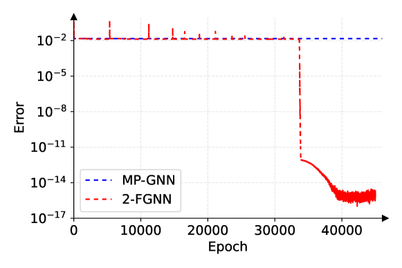
Figure 1. 2-FGNN can fit SB scores of MILP (3.1) and (3.2) simultaneously while MP-GNN can not.

6. Conclusion

In this work, we study the expressive power of two types of GNNs for representing SB scores. On one hand, MP-GNNs lack the separation power to distinguish all MILPs with different SB scores, and hence cannot perform well on some particular MILP datasets. On the other hand, 2-FGNNs, which update node-pair features instead of node features as in MP-GNNs, can universally approximate the SB scores on every MILP dataset or for every MILP distribution. Our results provide guidance on how to design suitable neural network structures for learning branching strategies, which could potentially be beneficial for modern MILP solvers.

We also comment on future research topics. Although the universal approximation result is established for 2-FGNNs and SB scores, it is still unclear what is the required complexity/number of parameters to achieve a given precision. It would thus be interesting and more practically useful to derive some quantitative results. In addition, our current numerical experiments are somehow of small-scale. Implementing large-scale experiments and exploring efficient training strategies could lead to more practical impacts.

Appendix A Proof of Theorem 4.2

Proof of Theorem 4.2.

It is clear that $G\stackrel{{\scriptstyle W}}{{\sim}}\sigma_{W}\ast\bar{G}$ implies that $G\sim\bar{G}$. We then prove the reverse direction, i.e., $G\sim\bar{G}$ implies $G\stackrel{{\scriptstyle W}}{{\sim}}\sigma_{W}\ast\bar{G}$ for some $\sigma_{W}\in S_{n}$. It suffices to consider $L$ and hash functions such that there are no collisons in Algorithm 1 and no strict color refinement in the $L$-th iteration when $G$ and $\bar{G}$ are the input, which means that two edges are assigned with the same color in the $L$-th iteration if and only if their colors are the same in the $(L-1)$-th iteration. For any $j_{1},j_{2},j_{1}^{\prime},j_{2}^{\prime}\in W$, it holds that

$$C_{L}^{WW}(j_{1},j_{2})=C_{L}^{WW}(j_{1}^{\prime},j_{2}^{\prime})$$

$$\implies \left\{\left\{(C_{L}^{VW}(i,j_{2}),C_{L}^{VW}(i,j_{1})):i\in V\right\}\right\}=\left\{\left\{(C_{L}^{VW}(i,j_{2}^{\prime}),C_{L}^{VW}(i,j_{1}^{\prime})):i\in V\right\}\right\}$$

$$\implies \left\{\left\{C_{L}^{VW}(i,j_{1}):i\in V\right\}\right\}=\left\{\left\{C_{L}^{VW}(i,j_{1}^{\prime}):i\in V\right\}\right\}\ \textup{and}$$

$$\left\{\left\{C_{L}^{VW}(i,j_{2}):i\in V\right\}\right\}=\left\{\left\{C_{L}^{VW}(i,j_{2}^{\prime}):i\in V\right\}\right\}.$$

Similarly, one has that

$$C_{L}^{WW}(j_{1},j_{2})=\bar{C}_{L}^{WW}(j_{1}^{\prime},j_{2}^{\prime})$$

$$\implies \left\{\left\{C_{L}^{VW}(i,j_{1}):i\in V\right\}\right\}=\left\{\left\{\bar{C}_{L}^{VW}(i,j_{1}^{\prime}):i\in V\right\}\right\}\ \textup{and}$$

$$\left\{\left\{C_{L}^{VW}(i,j_{2}):i\in V\right\}\right\}=\left\{\left\{\bar{C}_{L}^{VW}(i,j_{2}^{\prime}):i\in V\right\}\right\},$$

and that

$$\bar{C}_{L}^{WW}(j_{1},j_{2})=\bar{C}_{L}^{WW}(j_{1}^{\prime},j_{2}^{\prime})$$

$$\implies \left\{\left\{\bar{C}_{L}^{VW}(i,j_{1}):i\in V\right\}\right\}=\left\{\left\{\bar{C}_{L}^{VW}(i,j_{1}^{\prime}):i\in V\right\}\right\}\ \textup{and}$$

$$\left\{\left\{\bar{C}_{L}^{VW}(i,j_{2}):i\in V\right\}\right\}=\left\{\left\{\bar{C}_{L}^{VW}(i,j_{2}^{\prime}):i\in V\right\}\right\}.$$

Therefore, for any

$$\mathbf{C}\in\left\{\left\{\left\{C_{L}^{VW}(i,j):i\in V\right\}\right\}:j\in W\right\}\cup\left\{\left\{\left\{\bar{C}_{L}^{VW}(i,j):i\in V\right\}\right\}:j\in W\right\},$$

it follows from (4.2) that

(A.1) $$\begin{split}&\left\{\left\{C_{L}^{WW}(j_{1},j_{2}):\left\{\left\{C_{L}^{VW}(i,j_{1}):i\in V\right\}\right\}=\left\{\left\{C_{L}^{VW}(i,j_{2}):i\in V\right\}\right\}=\mathbf{C}\right\}\right\}\\ =&\left\{\left\{\bar{C}_{L}^{WW}(j_{1},j_{2}):\left\{\left\{\bar{C}_{L}^{VW}(i,j_{1}):i\in V\right\}\right\}=\left\{\left\{\bar{C}_{L}^{VW}(i,j_{2}):i\in V\right\}\right\}=\mathbf{C}\right\}\right\}.\end{split}$$

Particularly, the number of elements in the two multisets in (A.1) should be the same, which implies that

$$\#\left\{j\in W:\left\{\left\{C_{L}^{VW}(i,j):i\in V\right\}\right\}=\mathbf{C}\right\}=\#\left\{j\in W:\left\{\left\{\bar{C}_{L}^{VW}(i,j):i\in V\right\}\right\}=\mathbf{C}\right\},$$

which then leads to

$$\left\{\left\{\left\{\left\{C_{L}^{VW}(i,j):i\in V\right\}\right\}:j\in W\right\}\right\}=\left\{\left\{\left\{\left\{\bar{C}_{L}^{VW}(i,j):i\in V\right\}\right\}:j\in W\right\}\right\}.$$

One can hence apply some permutation on $W$ to obtain (4.3). Next we prove (4.4). For any $j\in W$, we have

$$\left\{\left\{C_{L}^{VW}(i,j):i\in V\right\}\right\}=\left\{\left\{\bar{C}_{L}^{VW}(i,j):i\in V\right\}\right\}$$

$$\implies C_{L}^{VW}(i_{1},j)=\bar{C}_{L}^{VW}(i_{2},j)\quad\textup{for some }i_{1},i_{2}\in V$$

$$\implies \left\{\left\{(C_{L}^{WW}(j_{1},j),C_{l-1}^{VW}(i_{1},j_{1})):j_{1}\in W\right\}\right\}=\left\{\left\{(\bar{C}_{L}^{WW}(j_{1},j),\bar{C}_{l-1}^{VW}(i_{2},j_{1})):j_{1}\in W\right\}\right\}$$

$$\qquad\qquad\textup{for some }i_{1},i_{2}\in V$$

$$\implies \left\{\left\{C_{L}^{WW}(j_{1},j):j_{1}\in W\right\}\right\}=\left\{\left\{\bar{C}_{L}^{WW}(j_{1},j):j_{1}\in W\right\}\right\},$$

which completes the proof. ∎

Appendix B Proof of Theorem 4.3

Theorem B.1.

For any $G,\bar{G}\in\mathcal{G}_{m,n}$, if $G\stackrel{{\scriptstyle W}}{{\sim}}\bar{G}$, then for any $j\in\{1,2,\dots,n\}$, $\hat{l}_{j}\in\{-\infty\}\cup\mathbb{R}$, and $\hat{u}_{j}\in\mathbb{R}\cup\{+\infty\}$, the two LP problems $\textup{LP}(G,j,\hat{l}_{j},\hat{u}_{j})$ and $\textup{LP}(\bar{G},j,\hat{l}_{j},\hat{u}_{j})$ have the same optimal objective value.

Theorem B.2 ([chen2022representing-lp]).

Consider two LP problems with $n$ variables and $m$ constraints

(B.1) $$\min_{x\in\mathbb{R}^{n}}~{}~{}c^{\top}x,\quad\textup{s.t.}~{}~{}Ax\circ b,~{}~{}l\leq x\leq u,$$

and

(B.2) $$\min_{x\in\mathbb{R}^{n}}~{}~{}\bar{c}^{\top}x,\quad\textup{s.t.}~{}~{}\bar{A}x\ \bar{\circ}\ \bar{b},~{}~{}\bar{l}\leq x\leq\bar{u}.$$

Suppose that there exist $\mathcal{I}=\{I_{1},I_{2},\dots,I_{s}\}$ and $\mathcal{J}=\{J_{1},J_{2},\dots,J_{t}\}$ that are partitions of $V=\{1,2,\dots,m\}$ and $W=\{1,2,\dots,n\}$ respectively, such that the followings hold:

1. For any $p\in\{1,2,\dots,s\}$, $(b_{i},\circ_{i})=(\bar{b}_{i},\bar{\circ}_{i})$ is constant over all $i\in I_{p}$;

2. For any $q\in\{1,2,\dots,t\}$, $(c_{j},l_{j},u_{j})=(\bar{c}_{j},\bar{l}_{j},\bar{u}_{j})$ is constant over all $j\in J_{q}$;

3. For any $p\in\{1,2,\dots,s\}$ and $q\in\{1,2,\dots,t\}$, $\sum_{j\in J_{q}}A_{ij}=\sum_{j\in J_{q}}\bar{A}_{ij}$ is constant over all $i\in I_{p}$.

4. For any $p\in\{1,2,\dots,s\}$ and $q\in\{1,2,\dots,t\}$, $\sum_{i\in I_{p}}A_{ij}=\sum_{i\in I_{p}}\bar{A}_{ij}$ is constant over all $j\in J_{q}$.

Then the two problems (B.1) and (B.2) have the same feasibility, the same optimal objective value, and the same optimal solution with the smallest $\ell_{2}$-norm (if feasible and bounded).

Proof of Theorem B.1.

Choose $L$ and hash functions such that there are no collisons in Algorithm 1 and no strict color refinement in the $L$-th iteration when $G$ and $\bar{G}$ are the input. Fix any $j\in W$ and construct the partions $\mathcal{I}=\{I_{1},I_{2},\dots,I_{s}\}$ and $\mathcal{J}=\{J_{1},J_{2},\dots,J_{t}\}$ as follows:

• $i_{1},i_{2}\in I_{p}$ for some $p\in\{1,2,\dots,s\}$ if and only if $C_{L}^{VW}(i_{1},j)=C_{L}^{VW}(i_{2},j)$.

• $j_{1},j_{2}\in J_{q}$ for some $q\in\{1,2,\dots,t\}$ if and only if $C_{L}^{WW}(j_{1},j)=C_{L}^{WW}(j_{2},j)$.

Without loss of generality, we can assume that $j\in J_{1}$. One observation is that $J_{1}=\{j\}$. This is because $j_{1}\in J_{1}$ implies that $C_{L}^{WW}(j_{1},j)=C_{L}^{WW}(j,j)$, which then leads to $C_{0}^{WW}(j_{1},j)=C_{0}^{WW}(j,j)$ and $\delta_{j_{1}j}=\delta_{jj}=1$ since there is no collisions. We thus have $j_{1}=j$.

Note that we have (4.3) and (4.4) from the assumption $G\stackrel{{\scriptstyle W}}{{\sim}}\bar{G}$. So after permuting $\bar{G}$ on $V$ and $W\backslash\{j\}$, one can obtain $C_{L}^{VW}(i,j)=\bar{C}_{L}^{VW}(i,j)$ for all $i\in V$ and $C_{L}^{WW}(j_{1},j)=\bar{C}_{L}^{WW}(j_{1},j)$ for all $j_{1}\in W$. Another observation is that such permutation does not change the optimal objective value of $\textup{LP}(\bar{G},j,\hat{l}_{j},\hat{u}_{j})$ as $j$ is fixed.

Next, we verify the four conditions in Theorem B.2 for two LP problems $\textup{LP}(G,j,\hat{l}_{j},\hat{u}_{j})$ and $\textup{LP}(\bar{G},j,\hat{l}_{j},\hat{u}_{j})$ with respect to the partitions $\mathcal{I}=\{I_{1},I_{2},\dots,I_{s}\}$ and $\mathcal{J}=\{J_{1},J_{2},\dots,J_{t}\}$.

Verification of Condition (a) in Theorem B.2.

Since there is no collision in the 2-FWL test Algorithm 1, $C_{L}^{VW}(i,j)=\bar{C}_{L}^{VW}(i,j)$ implies that $C_{0}^{VW}(i,j)=\bar{C}_{0}^{VW}(i,j)$ and hence that $v_{i}=\bar{v}_{i}$, which is also constant over all $i\in I_{p}$ since $C_{L}^{VW}(i,j)$ is contant over all $i\in I_{p}$ by definition.

Verification of Condition (b) in Theorem B.2.

It follows from $C_{L}^{WW}(j_{1},j)=\bar{C}_{L}^{WW}(j_{1},j)$ that $C_{0}^{WW}(j_{1},j)=\bar{C}_{0}^{WW}(j_{1},j)$ and hence that $w_{j_{1}}=\bar{w}_{j_{1}}$, which is also constant over all $j_{1}\in I_{q}$ since $C_{L}^{WW}(j_{1},j)$ is contant over all $j_{1}\in I_{q}$ by definition.

Verification of Condition (c) in Theorem B.2.

Consider any $p\in\{1,2,\dots,s\}$ and any $i\in I_{p}$. It follows from $C_{L}^{VW}(i,j)=\bar{C}_{L}^{VW}(i,j)$ that

$$\left\{\left\{(C_{L-1}^{WW}(j_{1},j),C_{L-1}^{VW}(i,j_{1})):j_{1}\in W\right\}\right\}=\left\{\left\{(\bar{C}_{L-1}^{WW}(j_{1},j),\bar{C}_{L-1}^{VW}(i,j_{1})):j_{1}\in W\right\}\right\},$$

and hence that

$$\left\{\left\{(C_{L}^{WW}(j_{1},j),A_{ij_{1}}):j_{1}\in W\right\}\right\}=\left\{\left\{(\bar{C}_{L}^{WW}(j_{1},j),\bar{A}_{ij_{1}}):j_{1}\in W\right\}\right\},$$

where we used the fact that there is no strict color refinement in the $L$-th iteration and there is no collision in Algorithm 1. We can thus conclude for any $q\in\{1,2,\dots,t\}$ that

$$\{\{A_{ij_{1}}:j_{1}\in J_{q}\}\}=\{\{\bar{A}_{ij_{1}}:j_{1}\in J_{q}\}\},$$

which implies that $\sum_{j_{1}\in J_{q}}A_{ij_{1}}=\sum_{j_{1}\in J_{q}}\bar{A}_{ij_{1}}$ that is constant over $i\in I_{p}$ since $C_{L}^{VW}(i,j)=\bar{C}_{L}^{VW}(i,j)$ is constant over $i\in I_{p}$.

Verification of Condition (d) in Theorem B.2.

Consider any $q\in\{1,2,\dots,t\}$ and any $j_{1}\in J_{q}$. It follows from $C_{L}^{WW}(j_{1},j)=\bar{C}_{L}^{WW}(j_{1},j)$ that

$$\left\{\left\{(C_{L-1}^{VW}(i,j),C_{L-1}^{VW}(i,j_{1})):i\in V\right\}\right\}=\left\{\left\{(\bar{C}_{L-1}^{VW}(i,j),\bar{C}_{L-1}^{VW}(i,j_{1})):i\in V\right\}\right\},$$

and hence that

$$\left\{\left\{(C_{L}^{VW}(i,j),A_{ij_{1}}):i\in V\right\}\right\}=\left\{\left\{(\bar{C}_{L}^{VW}(i,j),\bar{A}_{ij_{1}}):i\in V\right\}\right\},$$

where we used the fact that there is no strict color refinement at the $L$-th iteration and there is no collision in Algorithm 1. We can thus conclude for any $p\in\{1,2,\dots,s\}$ that

$$\{\{A_{ij_{1}}:i\in I_{p}\}\}=\{\{\bar{A}_{ij_{1}}:i\in I_{p}\}\},$$

which implies that $\sum_{i\in I_{p}}A_{ij_{1}}=\sum_{i\in I_{p}}\bar{A}_{ij_{1}}$ that is constant over $j_{1}\in J_{q}$ since $C_{L}^{WW}(j_{1},j)=\bar{C}_{L}^{WW}(j_{1},j)$ is constant over $j_{1}\in J_{q}$.

Combining all discussion above and noticing that $J_{1}=\{j\}$, one can apply Theorem B.2 and conclude that the two LP problems $\textup{LP}(G,j,\hat{l}_{j},\hat{u}_{j})$ and $\textup{LP}(\bar{G},j,\hat{l}_{j},\hat{u}_{j})$ have the same optimal objective value, which completes the proof. ∎

Corollary B.3.

For any $G,\bar{G}\in\mathcal{G}_{m,n}$, if $G\stackrel{{\scriptstyle W}}{{\sim}}\bar{G}$, then the LP relaxations of $G$ and $\bar{G}$ have the same optimal objective value and the same optimal solution with the smallest $\ell_{2}$-norm (if feasible and bounded).

Proof.

If no collision, it follows from (4.4) that $C_{L}^{WW}(j,j)=\bar{C}_{L}^{WW}(j,j)$ which implies $l_{j}=\bar{l}_{j}$ and $u_{j}=\bar{u}_{j}$ for any $j\in W$. Then we can apply Theorem B.1 to conclude that two LP problems $\textup{LP}(G,j,l_{j},u_{j})$ and $\textup{LP}(\bar{G},j,\bar{l}_{j},\bar{u}_{j})$ that are LP relaxations of $G$ and $\bar{G}$ have the same optimal objective value.

In the case that the LP relaxations of $G$ and $\bar{G}$ are both feasible and bounded, we use $x$ and $\bar{x}$ to denote their optimal solutions with the smallest $\ell_{2}$-norm. For any $j\in W$, $x$ and $\bar{x}$ are also the optimal solutions with the smallest $\ell_{2}$-norm for $\textup{LP}(G,j,l_{j},u_{j})$ and $\textup{LP}(\bar{G},j,\bar{l}_{j},\bar{u}_{j})$ respectively. By Theorem B.2 and the same arguments as in the proof of Theorem B.1, we have the $x_{j}=\bar{x}_{j}$. Note that we cannot infer $x=\bar{x}$ by considering a single $j\in W$ because we apply permutation on $V$ and $W\backslash\{j\}$ in the proof of Theorem B.1. But we have $x_{j}=\bar{x}_{j}$ for any $j\in W$ which leads to $x=\bar{x}$. ∎

Proof of Theorem 4.3.

(a) By Corollary B.3 and Theorem B.1.

(b) By Theorem 4.2 and (a).

(c) Apply (a) on $G$ and the graph obtained from $G$ by switching $j_{1}$ and $j_{2}$. ∎

Appendix C Proof of Theorem 4.4

Lemma C.1.

For any $G,\bar{G}\in\mathcal{G}_{m,n}$, if $G\stackrel{{\scriptstyle W}}{{\sim}}\bar{G}$, then $F(G)=F(\bar{G})$ for all $F\in\mathcal{F}_{\textup{2-FGNN}}$.

Proof.

Consider any $F\in\mathcal{F}_{\textup{2-FGNN}}$ with $L$ layers and let $s_{ij}^{l},t_{j_{1}j_{2}}^{l}$ and $\bar{s}_{ij}^{l},\bar{t}_{j_{1}j_{2}}^{l}$ be the features in the $l$-th layer of $F$. Choose $L$ and hash functions such that there are no collisons in Algorithm 1 when $G$ and $\bar{G}$ are the input. We will prove the followings by induction for $0\leq l\leq L$:

1. $C_{l}^{VW}(i,j)=C_{l}^{VW}(i^{\prime},j^{\prime})$ implies $s_{ij}^{l}=s_{i^{\prime}j^{\prime}}^{l}$.

2. $C_{l}^{VW}(i,j)=\bar{C}_{l}^{VW}(i^{\prime},j^{\prime})$ implies $s_{ij}^{l}=\bar{s}_{i^{\prime}j^{\prime}}^{l}$.

3. $\bar{C}_{l}^{VW}(i,j)=\bar{C}_{l}^{VW}(i^{\prime},j^{\prime})$ implies $\bar{s}_{ij}^{l}=\bar{s}_{i^{\prime}j^{\prime}}^{l}$.

4. $C_{l}^{WW}(j_{1},j_{2})=C_{l}^{WW}(j_{1}^{\prime},j_{2}^{\prime})$ implies $t_{j_{1}j_{2}}^{l}=t_{j_{1}^{\prime}j_{2}^{\prime}}^{l}$.

5. $C_{l}^{WW}(j_{1},j_{2})=\bar{C}_{l}^{WW}(j_{1}^{\prime},j_{2}^{\prime})$ implies $t_{j_{1}j_{2}}^{l}=\bar{t}_{j_{1}^{\prime}j_{2}^{\prime}}^{l}$.

6. $\bar{C}_{l}^{WW}(j_{1},j_{2})=\bar{C}_{l}^{WW}(j_{1}^{\prime},j_{2}^{\prime})$ implies $\bar{t}_{j_{1}j_{2}}^{l}=\bar{t}_{j_{1}^{\prime}j_{2}^{\prime}}^{l}$.

As the induction base, the claims (a)-(f) are true for $l=0$ since $\textup{HASH}_{0}^{VW}$ and $\textup{HASH}_{0}^{WW}$ do not have collisions. Now we assume that the claims (a)-(f) are all true for $l-1$ where $l\in\{1,2,\dots,L\}$ and prove them for $l$. In fact, one can prove the claim (a) for $l$ as follow:

$$C_{l}^{VW}(i,j)=C_{l}^{VW}(i^{\prime},j^{\prime})$$

$$\implies C_{l-1}^{VW}(i,j)=C_{l-1}^{VW}(i^{\prime},j^{\prime})\quad\textup{and}$$

$$\left\{\left\{(C_{l-1}^{WW}(j_{1},j),C_{l-1}^{VW}(i,j_{1})):j_{1}\in W\right\}\right\}=\left\{\left\{(C_{l-1}^{WW}(j_{1},j^{\prime}),C_{l-1}^{VW}(i^{\prime},j_{1})):j_{1}\in W\right\}\right\}$$

$$\implies s_{ij}^{l-1}=s_{i^{\prime}j^{\prime}}^{l-1}\quad\textup{and}\quad\left\{\left\{(t_{j_{1}j}^{l-1},s_{ij_{1}}^{l-1}):j_{1}\in W\right\}\right\}=\left\{\left\{(t_{j_{1}j^{\prime}}^{l-1},s_{i^{\prime}j_{1}}^{l-1}):j_{1}\in W\right\}\right\}$$

$$\implies s_{ij}^{l}=s_{i^{\prime}j^{\prime}}^{l}.$$

The proof of claims (b)-(f) for $l$ is very similar and hence omitted.

Using the claims (a)-(f) for $L$, we can conclude that

$$G\stackrel{{\scriptstyle W}}{{\sim}}\bar{G}$$

$$\implies \left\{\left\{C_{L}^{VW}(i,j):i\in V\right\}\right\}=\left\{\left\{\bar{C}_{L}^{VW}(i,j):i\in V\right\}\right\},\ \forall~{}j\in W,\ \textup{and}$$

$$\left\{\left\{C_{L}^{WW}(j_{1},j):j_{1}\in W\right\}\right\}=\left\{\left\{\bar{C}_{L}^{WW}(j_{1},j):j_{1}\in W\right\}\right\},\ \forall~{}j\in W$$

$$\implies \left\{\left\{s_{ij}^{L}:i\in V\right\}\right\}=\left\{\left\{\bar{s}_{ij}^{L}:i\in V\right\}\right\},\ \forall~{}j\in W,\ \textup{and}$$

$$\left\{\left\{t_{j_{1}j}^{L}:j_{1}\in W\right\}\right\}=\left\{\left\{\bar{t}_{j_{1}j}^{L}:j_{1}\in W\right\}\right\},\ \forall~{}j\in W$$

$$\implies r\left(\sum_{i\in V}s_{ij}^{L},\sum_{j_{1}\in W}t_{j_{1}j}^{L}\right)=r\left(\sum_{i\in V}\bar{s}_{ij}^{L},\sum_{j_{1}\in W}\bar{t}_{j_{1}j}^{L}\right),\ \forall~{}j\in W$$

$$\implies F(G)=F(\bar{G}),$$

which completes the proof. ∎

Lemma C.2.

For any $G,\bar{G}\in\mathcal{G}_{m,n}$, if $F(G)=F(\bar{G})$ for all $F\in\mathcal{F}_{\textup{2-FGNN}}$, then $G\stackrel{{\scriptstyle W}}{{\sim}}\bar{G}$.

Proof.

We claim that for any $L$ there exists $2$-FGNN layers for $l=0,1,2,\dots,L$, such that the followings hold true for any $0\leq l\leq L$ and any hash functions:

1. $s_{ij}^{l}=s_{i^{\prime}j^{\prime}}^{l}$ implies $C_{l}^{VW}(i,j)=C_{l}^{VW}(i^{\prime},j^{\prime})$.

2. $s_{ij}^{l}=\bar{s}_{i^{\prime}j^{\prime}}^{l}$ implies $C_{l}^{VW}(i,j)=\bar{C}_{l}^{VW}(i^{\prime},j^{\prime})$.

3. $\bar{s}_{ij}^{l}=\bar{s}_{i^{\prime}j^{\prime}}^{l}$ implies $\bar{C}_{l}^{VW}(i,j)=\bar{C}_{l}^{VW}(i^{\prime},j^{\prime})$.

4. $t_{j_{1}j_{2}}^{l}=t_{j_{1}^{\prime}j_{2}^{\prime}}^{l}$ implies $C_{l}^{WW}(j_{1},j_{2})=C_{l}^{WW}(j_{1}^{\prime},j_{2}^{\prime})$.

5. $t_{j_{1}j_{2}}^{l}=\bar{t}_{j_{1}^{\prime}j_{2}^{\prime}}^{l}$ implies $C_{l}^{WW}(j_{1},j_{2})=\bar{C}_{l}^{WW}(j_{1}^{\prime},j_{2}^{\prime})$.

6. $\bar{t}_{j_{1}j_{2}}^{l}=\bar{t}_{j_{1}^{\prime}j_{2}^{\prime}}^{l}$ implies $\bar{C}_{l}^{WW}(j_{1},j_{2})=\bar{C}_{l}^{WW}(j_{1}^{\prime},j_{2}^{\prime})$.

Such layers can be constructed inductively. First, for $l=0$, we can simply choose $p^{0}$ that is injective on $\{(v_{i},w_{j},A_{ij}):i\in V,j\in W\}\cup\{(\bar{v}_{i},\bar{w}_{j},\bar{A}_{ij}):i\in V,j\in W\}$ and $q^{0}$ that is injective on $\{(w_{j_{1}},w_{j_{2}},\delta_{j_{1}j_{2}}):j_{1},j_{2}\in W\}\cup\{(\bar{w}_{j_{1}},\bar{w}_{j_{2}},\delta_{j_{1}j_{2}}):j_{1},j_{2}\in W\}$.

Assume that the conditions (a)-(f) are true for $l-1$ where $1\leq l\leq L$, we aim to construct the $l$-th layer such that (a)-(f) are also true for $l$. Let $\alpha_{1},\alpha_{2},\dots,\alpha_{u}$ collect all different elements in $\{s_{ij}^{l-1}:i\in V,j\in W\}\cup\{\bar{s}_{ij}^{l-1}:i\in V,j\in W\}$ and let $\beta_{1},\beta_{2},\dots,\beta_{u^{\prime}}$ collect all different elements in $\{t_{j_{1}j_{2}}^{l-1}:j_{1},j_{2}\in W\}\cup\{\bar{t}_{j_{1}j_{2}}^{l-1}:j_{1},j_{2}\in W\}$. Choose some constinuous $f^{l}$ such that $f^{l}(\beta_{k^{\prime}},\alpha_{k})=e_{k^{\prime}}^{u^{\prime}}\otimes e_{k}^{u}\in\mathbb{R}^{u^{\prime}\times u}$, where $e_{k^{\prime}}^{u^{\prime}}$ is a vector in $\mathbb{R}^{u^{\prime}}$ with the $k^{\prime}$-th entry being $1$ and other entries being $0$, and $e_{k}^{u}$ is a vector in $\mathbb{R}^{u}$ with the $k$-th entry being $1$ and other entries being $0$. Choose some continuous $p^{l}$ that is injective on the set $\left\{s_{ij}^{l-1},\sum_{j_{1}\in W}f^{l}(t_{j_{1}j}^{l-1},s_{ij_{1}}^{l-1}):i\in V,j\in W\right\}\cup\left\{\bar{s}_{ij}^{l-1},\sum_{j_{1}\in W}f^{l}(\bar{t}_{j_{1}j}^{l-1},\bar{s}_{ij_{1}}^{l-1}):i\in V,j\in W\right\}$. By the injectivity of $p^{l}$ and the linear independence of $\{e_{k^{\prime}}^{u^{\prime}}\otimes e_{k}^{u}:1\leq k\leq u,1\leq k^{\prime}\leq u^{\prime}\}$, we have that

$$s_{ij}^{l}=s_{i^{\prime}j^{\prime}}^{l}$$

$$\implies s_{ij}^{l-1}=s_{i^{\prime}j^{\prime}}^{l-1}\quad\textup{and}\quad\sum_{j_{1}\in W}f^{l}(t_{j_{1}j}^{l-1},s_{ij_{1}}^{l-1})=\sum_{j_{1}\in W}f^{l}(t_{j_{1}j^{\prime}}^{l-1},s_{i^{\prime}j_{1}}^{l-1})$$

$$\implies s_{ij}^{l-1}=s_{i^{\prime}j^{\prime}}^{l-1}\quad\textup{and for any }1\leq k\leq u,\ 1\leq k^{\prime}\leq u^{\prime}$$

$$\#\big{\{}j_{1}\in W:t_{j_{1}j}^{l-1}=\beta_{k^{\prime}},s_{ij_{1}}^{l-1}=\alpha_{k}\big{\}}=\#\big{\{}j_{1}\in W:t_{j_{1}j^{\prime}}^{l-1}=\beta_{k^{\prime}},s_{i^{\prime}j_{1}}^{l-1}=\alpha_{k}\big{\}}$$

$$\implies s_{ij}^{l-1}=s_{i^{\prime}j^{\prime}}^{l-1}\quad\textup{and}\quad\big{\{}\big{\{}(t_{j_{1}j}^{l-1},s_{ij_{1}}^{l-1}):j_{1}\in W\big{\}}\big{\}}=\big{\{}\big{\{}(t_{j_{1}j^{\prime}}^{l-1},s_{i^{\prime}j_{1}}^{l-1}):j_{1}\in W\big{\}}\big{\}}$$

$$\implies C_{l-1}^{VW}(i,j)=C_{l-1}^{VW}(i^{\prime},j^{\prime})\quad\textup{and}$$

$$\Big{\{}\Big{\{}(C_{l-1}^{WW}(j_{1},j),C_{l-1}^{VW}(i,j_{1})):j_{1}\in W\Big{\}}\Big{\}}=\Big{\{}\Big{\{}(C_{l-1}^{WW}(j_{1},j^{\prime}),C_{l-1}^{VW}(i^{\prime},j_{1})):j_{1}\in W\Big{\}}\Big{\}}$$

$$\implies C_{l}^{VW}(i,j)=C_{l}^{VW}(i^{\prime},j^{\prime}),$$

which is to say that the condition (a) is satisfied. One can also verify that the conditions (b) and (c) by using the same argument. Similarly, we can also construct $g^{l}$ and $q^{l}$ such that the conditions (d)-(f) are satisfied.

Suppose that $G\stackrel{{\scriptstyle W}}{{\sim}}\bar{G}$ is not true. Then there exists $L$ and hash functions such that

$$\left\{\left\{C_{L}^{VW}(i,j):i\in V\right\}\right\}\neq\left\{\left\{\bar{C}_{L}^{VW}(i,j):i\in V\right\}\right\},$$

or

$$\left\{\left\{C_{L}^{WW}(j_{1},j):j_{1}\in W\right\}\right\}\neq\left\{\left\{\bar{C}_{L}^{WW}(j_{1},j):j_{1}\in W\right\}\right\},$$

holds for some $j\in W$. We have shown above that the conditions (a)-(f) are true for $L$ and some carefully constructed $2$-FGNN layers. Then it holds for some $j\in W$ that

(C.1) $$\left\{\left\{s_{ij}^{L}:i\in V\right\}\right\}\neq\left\{\left\{\bar{s}_{ij}^{L}:i\in V\right\}\right\},$$

or

(C.2) $$\left\{\left\{t_{j_{1}j}^{L}:j_{1}\in W\right\}\right\}\neq\left\{\left\{\bar{t}_{j_{1}j}^{L}:j_{1}\in W\right\}\right\}.$$

In the rest of the proof we work with (C.1), and the argument can be easily modified in the case that (C.2) is true. It follows from (C.1) that there exists some contiuous function $\varphi$ such that

$$\sum_{i\in V}\varphi(s_{ij}^{L})\neq\sum_{i\in V}\varphi(\bar{s}_{ij}^{L}).$$

Then let us construct the $(L+1)$-th layer yielding

$$s_{ij}^{L+1}=\varphi(s_{ij}^{L})\quad\textup{and}\quad\bar{s}_{ij}^{L+1}=\varphi(\bar{s}_{ij}^{L}),$$

and the output layer with

$$r\left(\sum_{i\in V}s_{ij}^{L+1},\sum_{j_{1}\in W}t_{j_{1}j}^{L+1}\right)=\sum_{i\in V}\varphi(s_{ij}^{L})\neq\sum_{i\in V}\varphi(\bar{s}_{ij}^{L})=r\left(\sum_{i\in V}\bar{s}_{ij}^{L+1},\sum_{j_{1}\in W}\bar{t}_{j_{1}j}^{L+1}\right).$$

This is to say $F(G)_{j}\neq F(\bar{G})_{j}$ for some $F\in\mathcal{F}_{\textup{2-FGNN}}$, which contradicts the assumtion that $F$ has the same output on $G$ and $\bar{G}$. Thus we can conclude that $G\stackrel{{\scriptstyle W}}{{\sim}}\bar{G}$. ∎

Proof of Theorem 4.4 (a).

By Lemma C.1 and Lemma C.2. ∎

Proof of Theorem 4.4 (b).

Apply Theorem 4.4 on $G$ and the graph obtained from $G$ by switching $j_{1}$ and $j_{2}$. ∎

Proof of Theorem 4.4 (c).

Suppose that $G\sim\bar{G}$. By Theorem 4.2, there exists some permutation $\sigma_{W}\in S_{n}$ such that $G\stackrel{{\scriptstyle W}}{{\sim}}\sigma_{W}\ast\bar{G}$. For any scalar function $f$ with $f\mathbf{1}\in\mathcal{F}_{\textup{2-FGNN}}$, by Theorem 4.4, it holds that $(f\mathbf{1})(G)=(f\mathbf{1})(\sigma_{W}\ast\bar{G})=(f\mathbf{1})(\bar{G})$, where we used the fact that $f\mathbf{1}$ is permutation-equivariant. We can thus conclude that $f(G)=f(\bar{G})$.

Now suppose that $G\sim\bar{G}$ is not true. Then there exist some $L$ and hash functions such that

$$\left\{\left\{C_{L}^{VW}(i,j):i\in V,j\in W\right\}\right\}\neq\left\{\left\{\bar{C}_{L}^{VW}(i,j):i\in V,j\in W\right\}\right\},$$

or

$$\left\{\left\{C_{L}^{WW}(j_{1},j_{2}):j_{1},j_{2}\in W\right\}\right\}\neq\left\{\left\{\bar{C}_{L}^{WW}(j_{1},j_{2}):j_{1},j_{2}\in W\right\}\right\}.$$

By the proof of Lemma C.2, one can construct the $l$-th $2$-FGNN layers inductively for $0\leq l\leq L$, such that the condition (a)-(f) in the proof of Lemma C.2 are true. Then we have

(C.3) $$\left\{\left\{s_{ij}^{L}:i\in V,j\in W\right\}\right\}\neq\left\{\left\{\bar{s}_{ij}^{L}:i\in V,j\in W\right\}\right\},$$

or

(C.4) $$\left\{\left\{t_{j_{1}j_{2}}^{L}:j_{1},j_{2}\in W\right\}\right\}\neq\left\{\left\{\bar{t}_{j_{1}j_{2}}^{L}:j_{1},j_{2}\in W\right\}\right\}.$$

We first assume that (C.3) is true. Then there exists a continuous function $\varphi$ with

$$\sum_{i\in V,j\in W}\varphi(s_{ij}^{L})\neq\sum_{i\in V,j\in W}\varphi(\bar{s}_{ij}^{L}).$$

Let us construct the $(L+1)$-th layer such that

$$s_{ij}^{L+1}=p^{L+1}\left(s_{ij}^{L},\sum_{j_{1}\in W}f^{L+1}(t_{j_{1}j}^{L},s_{ij_{1}}^{L})\right)=\sum_{j_{1}\in W}\varphi(s_{ij_{1}}^{L}),$$

$$\bar{s}_{ij}^{L+1}=p^{L+1}\left(\bar{s}_{ij}^{L},\sum_{j_{1}\in W}f^{L+1}(\bar{t}_{j_{1}j}^{L},\bar{s}_{ij_{1}}^{L})\right)=\sum_{j_{1}\in W}\varphi(\bar{s}_{ij_{1}}^{L}),$$

and the output layer with

$$r\left(\sum_{i\in V}s_{ij}^{L+1},\sum_{j_{1}\in W}t_{j_{1}j}^{L+1}\right)=\sum_{i\in V}\sum_{j_{1}\in W}\varphi(s_{ij_{1}}^{L})\neq\sum_{i\in V}\sum_{j_{1}\in W}\varphi(\bar{s}_{ij_{1}}^{L})=r\left(\sum_{i\in V}\bar{s}_{ij}^{L+1},\sum_{j_{1}\in W}\bar{t}_{j_{1}j}^{L+1}\right),$$

which is independent of $j\in W$. This constructs $F\in\mathcal{F}_{\textup{2-FGNN}}$ of the form $F=f\mathbf{1}$ with $f(G)\neq f(\bar{G})$.

Next we consider the case that (C.4) is true. Then

(C.5) $$\left\{\left\{\left\{\left\{t_{j_{1}j_{2}}^{L}:j_{1}\in W\right\}\right\}:j_{2}\in W\right\}\right\}\neq\left\{\left\{\left\{\left\{\bar{t}_{j_{1}j_{2}}^{L}:j_{1}\in W\right\}\right\}:j_{2}\in W\right\}\right\},$$

and hence there exists some continuous $\psi$ such that

$$\left\{\left\{\sum_{j_{1}\in W}\psi(t_{j_{1}j_{2}}^{L}):j_{2}\in W\right\}\right\}\neq\left\{\left\{\sum_{j_{1}\in W}\psi(\bar{t}_{j_{1}j_{2}}^{L}):j_{2}\in W\right\}\right\}.$$

Let us construct the $(L+1)$-th layer such that

$$s_{ij}^{L+1}=p^{L+1}\left(s_{ij}^{L},\sum_{j_{1}\in W}f^{L+1}(t_{j_{1}j}^{L},s_{ij_{1}}^{L})\right)=\sum_{j_{1}\in W}\psi(t_{j_{1}j}^{L}),$$

$$\bar{s}_{ij}^{L+1}=p^{L+1}\left(\bar{s}_{ij}^{L},\sum_{j_{1}\in W}f^{L+1}(\bar{t}_{j_{1}j}^{L},\bar{s}_{ij_{1}}^{L})\right)=\sum_{j_{1}\in W}\psi(\bar{t}_{j_{1}j}^{L}),$$

and we have from (C.5) that

$$\left\{\left\{s_{ij}^{L+1}:i\in V,j\in W\right\}\right\}\neq\left\{\left\{\bar{s}_{ij}^{L+1}:i\in V,j\in W\right\}\right\}.$$

We can therefore repeat the argument for (C.3) and show the existence of $f$ with $f\mathbf{1}\in\mathcal{F}_{\textup{2-FGNN}}$ and $f(G)\neq f(\bar{G})$. The proof is hence completed. ∎

Appendix D Proof of Theorem 3.2

Theorem D.1 (Lusin’s theorem [evans2018measure]*Theorem 1.14).

Suppose that $\mu$ is a Borel regular measure on $\mathbb{R}^{n}$ and that $f:\mathbb{R}^{n}\rightarrow\mathbb{R}^{m}$ is $\mu$-measurable, i.e., for any open subset $U\subset\mathbb{R}^{m}$, $f^{-1}(U)$ is $\mu$-measurable. Then for any $\mu$-measurable $X\subset\mathbb{R}^{n}$ with $\mu(X)<\infty$ and any $\epsilon>0$, there exists a compact set $E\subset X$ with $\mu(X\backslash E)<\epsilon$, such that $f|_{E}$ is continuous.

Theorem D.2 (Generalized Stone-Weierstrass theorem [azizian2020expressive]).

Let $X$ be a compact topology space and let $\mathbf{G}$ be a finite group that acts continuously on $X$ and $\mathbb{R}^{n}$. Define the collection of all equivariant continuous functions from $X$ to $\mathbb{R}^{n}$ as follows:

$$\mathcal{C}_{E}(X,\mathbb{R}^{n})=\{F\in\mathcal{C}(X,\mathbb{R}^{n}):F(g\ast x)=g\ast F(x),\ \forall~{}x\in X,g\in\mathbf{G}\}.$$

Consider any $\mathcal{F}\subset\mathcal{C}_{E}(X,\mathbb{R}^{n})$ and any $\phi\in\mathcal{C}_{E}(X,\mathbb{R}^{n})$. Suppose the following conditions hold:

1. $\mathcal{F}$ is a subalgebra of $\mathcal{C}(X,\mathbb{R}^{n})$ and $\mathbf{1}\in\mathcal{F}$, where $\mathbf{1}$ is the constant function whose ouput is always $(1,1,\dots,1)\in\mathbb{R}^{n}$.

2. For any $x,x^{\prime}\in X$, if $f(x)=f(x^{\prime})$ holds for any $f\in\mathcal{C}(X,\mathbb{R})$ with $f\mathbf{1}\in\mathcal{F}$, then for any $F\in\mathcal{F}$, there exists $g\in\mathbf{G}$ such that $F(x)=g\ast F(x^{\prime})$.

3. For any $x,x^{\prime}\in X$, if $F(x)=F(x^{\prime})$ holds for any $F\in\mathcal{F}$, then $\phi(x)=\phi(x^{\prime})$.

4. For any $x\in X$, it holds that $\phi(x)_{j}=\phi(x)_{j^{\prime}},\ \forall~{}(j,j^{\prime})\in J(x)$, where

   $$J(x)=\left\{\{1,2,\dots,n\}^{n}:F(x)_{j}=F(x)_{j^{\prime}},\ \forall~{}F\in\mathcal{F}\right\}.$$

Then for any $\epsilon>0$, there exists $F\in\mathcal{F}$ such that

$$\sup_{x\in X}\|F(x)-\phi(x)\|\leq\epsilon.$$

Proof of Theorem 3.2.

Lemma F.2 and Lemma F.3 in [chen2022representing-lp] prove that the function that maps LP instances to its optimal objective value/optimal solution with the smallest $\ell_{2}$-norm is Borel measurable. Thus, $\textup{SB}:\mathcal{G}_{m,n}\supset\textup{SB}^{-1}(\mathbb{R}^{n})\rightarrow\mathbb{R}^{n}$ is also Borel measurable, and is hence $\mathbb{P}$-measurable due to Assumption 3.1. By Theorem D.1 and Assumption 3.1, there exists a compact subset $X_{1}\subset\mathcal{G}_{m,n}$ such that $\mathbb{P}[\mathcal{G}_{m,n}\backslash X_{1}]\leq\epsilon$ and $\textup{SB}|_{X_{1}}$ is continuous. For any $\sigma_{V}\in S_{m}$ and $\sigma_{W}\in S_{n}$, $(\sigma_{V},\sigma_{W})\ast X_{1}$ is also compact and $\textup{SB}|_{(\sigma_{V},\sigma_{W})\ast X_{1}}$ is also continuous by the permutation-equivariance of BS. Set

$$X_{2}=\bigcup_{\sigma_{V}\in S_{m},\sigma_{W}\in S_{n}}(\sigma_{V},\sigma_{W})\ast X_{1}.$$

Then $X_{2}$ is permutation-invariant and compact with

$$\mathbb{P}[\mathcal{G}_{m,n}\backslash X_{2}]\leq\mathbb{P}[\mathcal{G}_{m,n}\backslash X_{1}]\leq\epsilon.$$

In addition, $\textup{SB}|_{X_{2}}$ is continuous by pasting lemma.

The rest of the proof is to apply Theorem D.2 for $X=X_{2}$, $\mathbf{G}=S_{m}\times S_{n}$, $\phi=\textup{SB}$, and $\mathcal{F}=\mathcal{F}_{\textup{2-FGNN}}$. We need to verify the four conditions in Theorem D.2. Condition (a) can be proved by similar arguments as in the proof of Lemma D.2 in [chen2022representing-lp]. Condition (b) follows directly from Theorem 4.4 (a) and (c) and Theorem 4.2. Condition (c) follows directly from Theorem 4.4 (a) and Theorem 4.3 (a). Condition (d) follows directly from Theorem 4.4 (b) and Theorem 4.3 (c). According to Theorem D.2, there exists some $F\in\mathcal{F}_{\textup{2-FGNN}}$ such that

$$\sup_{G\in X_{2}}\|F(G)-\textup{SB}(G)\|\leq\delta.$$

Therefore, one has

$$\mathbb{P}[\|F(G)-\textup{SB}(G)\|>\delta]\leq\mathbb{P}[\mathcal{G}_{m,n}\backslash X_{2}]\leq\epsilon,$$

which completes the proof. ∎