Quantum reservoir probing of quantum phase transitions

Abstract

Quantum phase transitions are highly remarkable phenomena manifesting in quantum many-body systems. However, their precise identifications in equilibrium systems pose significant theoretical and experimental challenges. Thus far, nonequilibrium detection protocols utilizing global quantum quenches have been proposed, yet the real-time signatures of these transitions are imprinted in intricate spatiotemporal correlations, compromising the simplicity and versatility of the protocols. Here, we propose a framework for dynamical detection of quantum phase transitions based on local quantum quenches. While the resultant dynamics are influenced by both the local quench operation and the intrinsic dynamics of the quantum system, the effects of the former are exclusively extracted through the cutting-edge framework called quantum reservoir probing (QRP). We illustrate that the impacts of the local quenches vary across different quantum phases, and are subdued by intrinsic fluctuations amplified in proximity to quantum critical points. Consequently, the QRP can detect quantum phase transitions in the paradigmatic integrable and nonintegrable quantum systems, all while utilizing single-site operators. Furthermore, we also show that topological quantum phase transitions can be detected using the identical framework. The broad applicability of the QRP, along with its experimental feasibility and design flexibility, highlights its universal effectiveness in identifying various quantum phase transitions.

INTRODUCTION

Quantum phase transitions emerge as quintessential manifestations of the interplay among quantum many-body phenomena [1, 2]. They are characterized by the universal description across microscopically different systems, which has been central to our understanding of quantum matters. Nevertheless, precisely detecting these transitions in equilibrium systems poses significant challenges both theoretically and experimentally, due to the limitations of computational resources for quantum simulations and the exponential time required to bring quantum systems into equilibrium near quantum critical points, respectively. This has led recent investigations to focus on nonequilibrium dynamics, which is inherently related to quantum phase transitions through dynamical critical phenomena. Indeed, real-time signatures of quantum phase transitions have been identified in a range of systems, from integrable to chaotic, through the analysis of out-of-time-order correlators [3, 4, 5, 6, 7] and generalized correlations and susceptibilities [8, 9, 10]. A commonly adopted strategy in these explorations is the implementation of a global quantum quench, wherein the entire system is initially configured in a specific state and subsequently experiences complex time evolution by the Hamiltonian dynamics. Recent experimental advancements in isolating and manipulating quantum systems have facilitated such sophisticated control in various platforms, including trapped ions [11, 12, 13, 14], ultracold atoms [15, 16, 17, 18], Rydberg atoms [19, 20, 21, 22], and nitrogen-vacancy centers [23]. Fundamentally, different quantum phases are discerned by spatiotemporal correlations of multiple operators after the global quench, though these measurements often present considerable technical challenges, which significantly constrains their applicabilities.

A pertinent question then emerges regarding the system response to a local quantum quench, introduced through localized quantum manipulation [24, 25, 26]. In contrast to its global counterpart, the local quench operation selectively influences nontrivial excitations or quasiparticles in specific regions of the system, thereby presenting itself as a potential universal protocol for exploring quantum phenomena, including the identification of quantum phase transitions. However, the complexity arises from the fact that the dynamics is not exclusively influenced by the quench operation, but also by the intrinsic dynamics of the quantum system itself. This multifaceted influence introduces a significant challenge in isolating and analyzing the response in the dynamics directly ascribed to the quench operation. While this complexity is inherent in both global and local quench scenarios, it becomes particularly critical in the case of local quenches, as these complicated effects obscure the potential benefit of local quenches in facilitating access to localized physics.

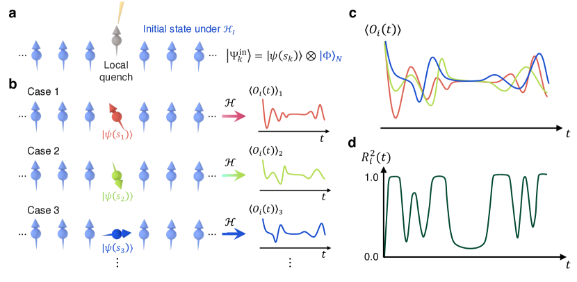
Figure 1: Conceptualization of the QRP. a Preparation and local manipulation to construct the initial state $|\Psi^{\mathrm{in}}_{k}\rangle$. The gray spin is manipulated by a local magnetic field applied by the yellow needle, while other spins are prepared in the ground state $|\Phi_{N}\rangle$ of the Hamiltonian $\mathcal{H}_{I}$ for the $N$-site system, illustrated here as an all-up state. b Diagrammatic representation of the initial quantum state for the $N+1$ spins [Eq. (1)]. The manipulated spin, characterized by the input vale $s_{k}$ for each case, is placed at the center of the system. This manipulation leads to a local operator $O_{i}(t)$ exhibiting varied dynamics that is reflective of the corresponding input values. c The dynamics of $\langle O_{i}(t)\rangle$ summarized across three cases depicted in (b). d Schematic illustration of the determination coefficient $R_{i}^{2}(t)$ derived from $\langle O_{i}(t)\rangle$. An almost unity $R^{2}_{i}(t)$ signifies a precise estimation of the input value, indicating the pronounced input-sensitivity of the observed $\langle O_{i}(t)\rangle$ [Eq. (5)]. Conversely, $R^{2}_{i}(t)$ approaches $0$ when $\langle O_{i}(t)\rangle$ exhibits similar values that do not reflect each input, as exemplified by intersections of $\langle O_{i}(t)\rangle$.

In this paper, we develop a general framework aimed at detecting quantum phase transitions through the response to a local quantum quench, which closely encapsulates the distinct characteristics of each quantum phase. For this purpose, we substantially enhance the methodology of “quantum reservoir probing” (QRP), initially proposed in Ref. [27], by expanding its applicability to pure quantum states. To elaborate, starting from a predefined global quantum state, we apply a random quench to a local degree of freedom and simulate the resultant dynamics; this process is repeated across numerous instances, followed by a comparative analysis among them. In scenarios where an operator is completely unaffected from this local quench operation, its response remains uniform despite the randomness introduced. Conversely, when affected, it manifests a varied response reflecting the randomness in quenching. Hence, the impacts of the local quench can be identified from the degree of deviation in the dynamics of operators. Upon this concept, the QRP framework statistically investigates the dependency of the subsequent dynamics on the randomness of the local quench operation. We demonstrate that the responses of even a single-site operator exhibits distinct variations depending on the inherent characteristics of the quantum phases, accompanied by universal anomalies appearing at the quantum critical point due to the enhanced fluctuations. This observation highlights the capability of our QRP to effectively detect quantum phase transitions with a notable advantage in terms of simplicity; it does not necessitate the measurement of complex spatiotemporal correlations, and can be implemented on experimentally feasible setups. Furthermore, notwithstanding the use of a single-site operator, we demonstrate the efficacy of our QRP in identifying topological quantum phase transitions, which are typically distinguished by the absence of local order parameters beyond the Landau-Gintzburg-Wilson paradigm. The broad applicability and design flexibility of our QRP establish it as a versatile tool for probing quantum phenomena, opening the door to further understanding of quantum many-body physics.

RESULTS

Framework of the QRP

First, let us overview the framework of QRP that we enhance for the application to a pure quantum state. The core principle underlying the QRP is the manipulation of a local degree of freedom from a specific quantum state. This quantum manipulation is dictated by a random input value $s_{k}$. Our focus is on a local operator $O$ defined per site $i$ and time $t$, denoted as $O_{i}(t)$, with particular attention to the variations induced by the input variable $s_{k}$. In the statistical analysis across various instances with different inputs subscripted by $k$, the expectation value $\langle O_{i}(t)\rangle_{k}$ may display diverse characteristics that closely reflect the corresponding input values. In such cases, the value of $s_{k}$ can be precisely deduced from $\langle O_{i}(t)\rangle_{k}$ through straightforward calculations. Hence, the successful estimation of the original input value $s_{k}$ provides evidence that the local manipulation exerts a significant influence on the operator $O_{i}(t)$ at that particular spatiotemporal coordinate. In contrast, the operator $O_{j}(t^{\prime})$ at a different spatiotemporal point may demonstrate consistent behavior across all instances, not accurately mirroring the local quench operation. In this latter case, the operator is predominantly governed by the inherent characteristics of the quantum system independent of the local quench. Therefore, the spatiotemporal dependency of the operator $O_{i}(t)$ on the input value $s_{k}$ explores how the local quantum quench influences the operator, while isolating it from other intrinsic phenomena. Remarkably, this linkage is highly sensitive to the Hamiltonian governing the quantum system. Thus, the operator’s dependency on the local quench operation serves as a witness to the properties of the quantum system, shedding light on the underlying quantum processes at play.

Here, we explain the specific procedures of the QRP on the one-dimensional (1D) quantum spin-$1/2$ systems. The protocol consists of four steps: (i) the preparation of the initial state based on the initial Hamiltonian $\mathcal{H}_{I}$ (Fig. 1a), (ii) the manipulated spin, parameterized by the input value $s_{k}$, is placed in the system (Figs. 1a and 1b), (iii) the observation of the dynamics of a local operator $\langle O_{i}(t)\rangle$ under the evolution Hamiltonian $\mathcal{H}$ (Figs. 1b and 1c), and (iv) the evaluation of the performance in estimating the respective input value $s_{k}$ from the observed dynamics, quantified via the determination coefficient $R_{i}^{2}(t)$ (Fig. 1d). We provide a comprehensive description of each step in the following.

First, the system is configured so that the manipulated spin remains disentangled from all other sites, ensuring its unrestricted manipulability. This setup is always straightforward for product states, but in general, it requires the isolation of the spin being manipulated from the rest of the system. For simplicity, we initially prepare the $N$-site system in the ground state of the initial Hamiltonian $\mathcal{H}_{I}$ in step (i). Then, in step (ii), the manipulated spin is placed in the system, forming the initial state for the ($N+1$)-site system (Fig. 1a); see Methods section. The resulting state is expressed as

$$|\Psi_{k}^{\mathrm{in}}\rangle=|\psi(s_{k})\rangle\otimes|\Phi\rangle_{N},$$ (1)

where $|\Phi\rangle_{N}$ represents the prepared initial state for the $N$-site subsystem, while $|\psi(s_{k})\rangle$ denotes the state of the manipulated spin (Fig. 1b). The input value $s_{k}$ is randomly sampled from a uniform distribution, specifically $s_{k}\in[0,1]$, which is encoded into the initial state. We here consider the all-up state shown in Fig. 1a for $|\Phi\rangle_{N}$ as a representative case, and express the initial state of the manipulated spin as

$$|\psi(s_{k})\rangle=\sqrt{1-s_{k}}|+\rangle+\sqrt{s_{k}}|-\rangle,$$ (2)

where $|\pm\rangle=\left(\mid\uparrow\rangle\pm\mid\downarrow\rangle\right)/\sqrt{2}$. We note that this state $|\psi(s_{k})\rangle$ can be prepared by applying a local magnetic field

$$\bm{h}\propto\left(2s_{k}-1,0,-2\sqrt{s_{k}(1-s_{k})}\right)$$ (3)

on the manipulated spin, with the field being subsequently deactivated following the state preparation of Eq. (1).

We then let the system to evolve under the Hamiltonian $\mathcal{H}$ for the entire ($N+1$)-site system in step (iii), resulting in the state $|\Psi_{k}(t)\rangle=e^{-i\mathcal{H}t}|\Psi_{k}^{\mathrm{in}}\rangle$; see Methods section. The expectation value of a local operator $O_{i}(t)$ is calculated as $\langle O_{i}(t)\rangle_{k}=\langle\Psi_{k}(t)|O_{i}|\Psi_{k}(t)\rangle$; we omit the subscript $k$ unless necessary. By iterating this procedure across various instances with different $s_{k}$, we generate multiple time series of the dynamics, as illustrated in Fig. 1c.

Finally in step (iv), we assess the influence of the local quantum quench on the local operator following the standard methodology used in physical reservoir computing [28, 29, 30, 31, 27]. Specifically, as a criterion for establishing a linkage between them, we employ the precision in estimating the input value $s_{k}$ through the linear transformation of $\langle O_{i}(t)\rangle_{k}$. For a given instance $k$, the output of this linear transformation is derived as

$$y_{i,k}(t)=w_{i,O}(t)\langle O_{i}(t)\rangle_{k}+w_{i,c}(t),$$ (4)

where $w_{i,O}(t)$ and $w_{i,c}(t)$ represent the $k$-independent coefficients. These weights are finely tuned for training instances so that the output $y_{{i,k}}(t)$ approximates the original input value $s_{k}$ as closely as possible over all $k$, based on the least squares method. Subsequently in the testing phase, the estimation performance for unknown instances is quantified by the determination coefficient

$$R_{i}^{2}(t)=\frac{\mathrm{cov}^{2}(\{y_{{i,k}}(t)\},\{s_{k}\})}{\sigma^{2}(\{y_{{i,k}}(t)\})\sigma^{2}(\{s_{k}\})},$$ (5)

where $\mathrm{cov}$ and $\sigma^{2}$ represent covariance and variance, respectively; see Methods section for more details. The value of $R^{2}_{i}(t)$ ranges between $0$ and $1$, with an approach towards $1$ indicating that $\{y_{{i,k}}(t)\}$ closely reproduces $\{s_{k}\}$ for all testing cases.

Figures 1c and 1d visually elucidate the relationship between the dynamics of $\langle O_{i}(t)\rangle$ and the corresponding $R^{2}_{i}(t)$. A high $R^{2}_{i}(t)$ value suggests that $\langle O_{i}(t)\rangle$ varies systematically in response to the input value $s_{k}$. In contrast, $R^{2}_{i}(t)$ close to $0$ indicates that $\langle O_{i}(t)\rangle$ is largely independent of $s_{k}$, such as at the crossing points resulting from inherent oscillations in the quantum system. Therefore, $R^{2}_{i}(t)$ serves as an indicator of the extent to which $O_{i}(t)$ is influenced by the local quench operation. It is worth emphasizing that restricting the transformation generating $y_{{i,k}}(t)$ from $\langle O_{i}(t)\rangle_{k}$ to a linear form is crucial; any additional nonlinearity could lead to either an overestimation or underestimation of the degree to which the effects of the local quench are reflected within the operator $O_{i}(t)$. Under different parameters of the Hamiltonian $\mathcal{H}$, the local quench operation exerts varying influences on the resultant dynamics, hence the spatiotemporal behavior of $R^{2}_{i}(t)$ are instrumental in examining the unique properties of each quantum phase.

Transverse-field Ising model

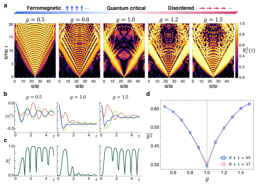
Figure 2: Identifying the quantum phase transition in the transverse-field Ising model via the QRP. a Spatiotemporal representation of the performance for the estimation of the input value. The color represents the value of $R^{2}_{i}(t)$ derived from $\langle\sigma^{x}_{i}(t)\rangle$. The upper band represents the schematic phase diagram regarding $\mathcal{H}(g)$, where the quantum critical point separating the ferromagnetically ordered phase and the quantum disordered phase exists at ${g_{c}}=1$. The system size is $N+1=49$, and the time evolution is calculated using a bond dimension $\chi=256$; the result is quantitatively the same for $\chi=128$. b The early-time spin dynamics at the nearest-neighbor site from the central one under three different input values. c The estimation performance $R^{2}_{i}(t)$ utilizing $\langle\sigma^{x}_{i}(t)\rangle$ at the same site as (b). d The average $\overline{R^{2}}$ over spatiotemporal indices $(i,t)\in\Lambda\times\{0<t\leq 10\}$, with $\Lambda$ encompassing the central $11$ sites. The blue and pink lines represent the system sizes $N+1=49$ and $N+1=37$, respectively. The quantum critical point is denoted by the gray dashed line.

Let us first apply our QRP protocol to the paradigmatic 1D Ising model with a transverse magnetic field under the open boundary condition. The Hamiltonian is given by

$$\mathcal{H}=-J\sum_{i}\sigma^{z}_{i}\sigma^{z}_{i+1}+g\sum_{i}\sigma^{x}_{i},$$ (6)

where ${\sigma}_{i}^{x}$ and ${\sigma}_{i}^{z}$ are the $x$ and $z$ Pauli matrices at site $i$, respectively. $g$ signifies the magnitude of the transverse magnetic field and $J>0$ denotes the strength of the nearest-neighbor ferromagnetic interaction; we set $J=1$ as our energy scale. This model manifests a quantum phase transition at the quantum critical point $g_{c}=1$ in the thermodynamic limit, which separates a ferromagnetically ordered phase for $g<1$ from a quantum disordered phase for $g>1$ [32, 1]. Notably, the model is solvable through the Jordan-Wigner transformation and the subsequent Bogoliubov transformation, where the spin system is mapped to the free quasiparticle picture [1].

We initialize $|\Phi\rangle_{N}$ as the ground state of $\mathcal{H}_{I}=\mathcal{H}(g=0)$, with introducing an infinitesimally small magnetic field to select the all-up state from the doubly degenerate ferromagnetic states. After placing the manipulated spin as the central spin, the constructed state $|\Psi^{\mathrm{in}}_{k}\rangle$ in Eq. (1) is explicitly formulated as:

$$|\Psi^{\mathrm{in}}_{k}\rangle=|\psi(s_{k})\rangle\otimes\mid\uparrow\uparrow\uparrow\dots\rangle_{N}.$$ (7)

Subsequently, we monitor the dynamics of the local spin $\langle\sigma^{x}_{i}(t)\rangle$ at each site $i$ under the evolution Hamiltonian $\mathcal{H}=\mathcal{H}(g)$ for the $(N+1)$-site system. Repeating the procedure for many instances, the estimation performance $R^{2}_{i}(t)$ in Eq. (5) is methodically evaluated.

Figure 2 encapsulates the results of the QRP under various magnetic fields $g$ for the evolution Hamiltonian after the quench, $\mathcal{H}(g)$. In Fig. 2a, we represent the spatiotemporal representation of the estimation performance $R^{2}_{i}(t)$, which reveals a discernible light-cone structure emanating from the manipulated central site. This spatiotemporal distribution of nonzero $R^{2}_{i}(t)$ suggests that the local spin operator $\langle\sigma_{i}^{x}(t)\rangle$ across diverse spatial locations and temporal moments adequately reflect the impact of the local quantum manipulation. The wavefronts observed are attributed to the propagation of the lowest-energy excitation along the $x$ axis in spin space, triggered by the manipulation at the central spin [Eq. (2)]. Indeed, pronounced $R^{2}_{i}(t)$ values in proximity to the wavefronts are especially conspicuous in the quantum disordered phase, reflecting the nature of the ground state with spins aligned in the $x$ direction. Following the traversal of the wavefront, the effects of the quench operation are imparted onto the quasiparticles, manifesting as alterations in phase and amplitude. This influence is evidenced by the nonzero values of $R^{2}_{i}(t)$, which appear as ripple-like patterns between wavefronts in both directions. An exception occurs near the quantum critical point at $g_{c}=1$ characterized by maximized fluctuations, which lead to an effective breakdown of the quasiparticle picture. Here, the effects of the quench operation are passed on the intrinsic fluctuations of the system, though such influences rapidly diminish as indicated by the noticeably small $R^{2}_{i}(t)$ after the passage of the wavefront. This observation highlights an anomalous suppression of information propagation at the quantum critical point, which is distinct from other non-critical phases.

In Fig. 2b, the early-time dynamics of $\langle\sigma^{x}_{i}(t)\rangle$ at the nearest-neighbor spin from the central one is depicted for three distinct input values $s_{k}$ at different magnetic fields $g$. At $g=0.5$ and $1.5$, the quasiparticles induce periodic spin oscillations, the phase and amplitude of which are dependent on the input $s_{k}$. In contrast, at $g=1.0$, the dynamics of $\langle\sigma^{x}_{i}(t)\rangle$ exhibits significant variation when the wavefronts pass at approximately $t\simeq 1$, thereafter stabilizing into a uniform pattern that does not reflect the influence of quench operation. Figure 2c displays the corresponding estimation performance at the same site (a vertical cross-section of the color map in Fig. 2a). Over broad temporal spans at $g=0.5$ and $1.5$, $R^{2}_{i}(t)$ becomes close to $1$, which statistically underscores the input dependency of the phase and amplitude of the spin oscillations. Conversely, its frequency is governed not by the manipulation of the initial state, but rather by the intrinsic characteristics of the quasiparticles themselves, as evidenced by $R^{2}_{i}(t)$ periodically approaching $0$ (Fig. 2c) at points where oscillations of $\langle\sigma_{i}^{x}(t)\rangle$ intersect for different inputs (Fig. 2b). Remarkably, at $g=1.0$, while $R^{2}_{i}(t)$ nears $1$ around $t\simeq 1$ where the wavefronts induce variations in the spin dynamics, the similarity of $\langle\sigma_{i}^{x}(t)\rangle$ in other temporal regions leads to $R^{2}_{i}(t)\simeq 0$, signifying the reduced influence of the local quench by the intrinsic fluctuations enhanced near the quantum critical point.

As described above, the relationship between the local quench operation and their resultant quantum dynamics of local operators manifests qualitatively and quantitatively different characteristics across different phases (Fig. 2a). The distribution of $R^{2}_{i}(t)$ thus serves as a marker for identifying the quantum phase transition. In Fig. 2d, we display the mean value of $R^{2}_{i}(t)$ over a specific subset of spatiotemporal indices $\{(i,t)\}$, denoted as $\overline{R^{2}}$. To minimize the effects from the edges of the system, this analysis focus on $(i,t)$ within the central eleven sites during the time interval $0<t\leq 10$, prior to any reflective effects; selecting different subsets does not qualitatively alter the results (see the Supplemental Information). As $g$ approaches $g_{c}=1$ from the ferromagnetically ordered state, the fluctuations are progressively intensified and interfere with the estimation of the original input, resulting in a decrease in $\overline{R^{2}}$. At the quantum critical point, $\overline{R^{2}}$ reaches its minimum, which corresponds to the emergence of a dark region between the wavefronts observed in Fig. 2a for $g=1.0$. Upon further augmentation of $g$ into the quantum disordered phase, the fluctuations are again suppressed and the effects of the quench operation become dominant, leading to an increase in $\overline{R^{2}}$. Therefore, the pronounced dip in Fig. 2d represents a definitive indicator of the quantum phase transition occurring at $g_{c}$. Consequently, by focusing on the variation in response to the local quench operation, our QRP successfully detects the quantum phase transition only by measurements of single-site spin dynamics.

Anisotropic next-nearest-neighbor Ising model

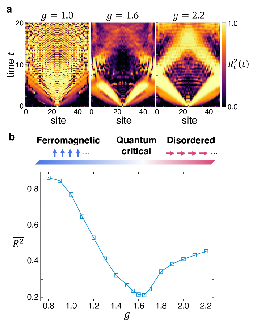
Figure 3: Detection of the quantum phase transition in the ANNNI model using the QRP. a Spatiotemporal representation of the estimation performance when employing $\langle\sigma^{x}_{i}(t)\rangle$ in a nonintegrable ANNNI chain characterized by an interaction parameter $\kappa=0.5$. The system size is $N+1=49$, and the time evolution is calculated with a bond dimension of $\chi=128$. b The average $\overline{R^{2}}$ over a subset $(i,t)\in\Lambda\times\{0<t\leq 15\}$, where $\Lambda$ contains the central eleven sites. The upper band represents the schematic phase diagram, where the ferromagnetically ordered and quantum disordered phases are separated by the quantum critical point at approximately $g\simeq 1.6$.

To illustrate the applicability of our QRP framework to nonintegrable models, we extend the model to the anisotropic next-nearest-neighbor Ising (ANNNI) chain [33, 34, 35]. The Hamiltonian is given by

$$\mathcal{H}=-J\sum_{i}\sigma^{z}_{i}\sigma^{z}_{i+1}-\kappa\sum_{i}\sigma^{z}_{i}\sigma^{z}_{i+2}+g\sum_{i}\sigma^{x}_{i},$$ (8)

where we take $J=1$ and $\kappa$ represents the strength of the next-nerarest-neighbor interaction. The latter term makes the system nonintegrable by introducing the four-body interactions for the quasiparticles derived by the Jordan-Wigner transformation. This model hosts a rich phase diagram in the $\kappa$-$g$ plane [36]. Our investigation focuses on the case of $\kappa=0.5$, where the quantum phase transition occurs at $g_{c}\simeq 1.6$ with the Ising universality, separating ferromagnetically ordered ($g<g_{c}$) and quantum disordered ($g>g_{c}$) phases. The initial state is prepared in the same manner as Eq. (7).

Figure 3a displays the spatiotemporal representation of $R^{2}_{i}(t)$ obtained from $\langle\sigma^{x}_{i}(t)\rangle$, revealing a scenario similar to the transverse-field Ising model. For the majority of sites and times, the local spin $\langle\sigma_{i}^{x}(t)\rangle$ mirrors the input value $s_{k}$ employed in the local quantum quench, as evidenced by the nonzero values of $R^{2}_{i}(t)$. Above the critical field at $g_{c}\simeq 1.6$, particularly for $g=2.2$ in the right panel, the effects of the local manipulation propagate primarily through the excitation wavefronts, while the local spin oscillations exhibit weaker dependence on the manipulation with small $R^{2}_{i}(t)$. Conversely, below the critical point the opposite behavior is noted in the left panel for $g=1.0$. Furthermore, in the vicinity of the quantum critical point, the influence of the local operation manifest itself predominantly along the wavefronts, while in the other regions it is suppressed by the enhanced fluctuations, as demonstrated by the emergence of a discernible dark zone between the wavefronts. Consequently, while the presence of next-nearest-neighbor coupling broadens the wavefronts for $g>g_{c}$ and interferes the oscillation periodicity for $g<g_{c}$, the fundamental dependencies of the local spin operators on the local quench operation retain a similarity to those observed in the integrable model presented in Fig. 2a.

In Fig. 3b, we present the mean value $\overline{R^{2}}$, calculated over the indices $(i,t)$ corresponding to the central eleven sites within the time frame $0<t\leq 15$ (see the Supplemental Information for other subsets). Analogous to the observation in Fig. 2d, $\overline{R^{2}}$ demonstrates a pronounced decrease around the quantum critical point at $g\simeq 1.6$, indicating the boundary between the different spatiotemporal distribution patterns of $R^{2}_{i}(t)$ in the ferromagnetically ordered phase and the quantum disordered phase. This observation confirms that, even in nonintegrable systems, $R^{2}_{i}(t)$ is an effective marker for detecting quantum phase transitions.

Spin-1 XXZ model

The preceding sections have demonstrated the effectiveness of our QRP framework in identifying quantum phase transitions, particularly between conventional phases where the internal physics is well-characterized and understood within the Landau-Ginzburg-Wilson theory. Building on this foundation, we now aim to broaden our exploration to more complex quantum phenomena. In particular, we apply the QRP framework to the detection of topological quantum phase transitions, which lack local order parameters that can distinguish adjacent phases. This raises the question of whether the QRP framework, which solely utilizes a single-site spin operator, can still be effective in identifying these transitions beyond the Landau-Gintzburg-Wilson paradigm.

Here, we study the spin-$1$ XXZ model with open boundaries [37, 38], which is defined by

$$\mathcal{H}=\sum_{i}J(S^{x}_{i}S^{x}_{i+1}+S^{y}_{i}S^{y}_{i+1})+\lambda S^{z}_{i}S^{z}_{i+1},$$ (9)

where $S^{\alpha}_{i}$ denotes the $\alpha$-component of spin-$1$ operator at site $i$ and $\lambda$ represents the Ising anisotropy; we set $J=1$. This model is renowned for hosting a prototypical symmetry-protected topological phase, known as the Haldane phase, observed for the anisotropy within $0<\lambda<\lambda_{c}$ with $\lambda_{c}\simeq 1.18$ [39, 40, 41]. The Haldane phase is distinguished by its protection under a $Z_{2}\times Z_{2}$ symmetry, and is characterized by nonlocal string order parameters [42, 43, 44]. With increasing the anisotropy, the topological quantum phase transition into the topologically trivial spin-$1$ Néel state occurs at the quantum critical point, which belongs to the two-dimensional (2D) Ising universality class [40, 45, 46].

The QRP framework can be naturally extended to the spin-$1$ XXZ model. Here, $|\Phi\rangle_{N}$ is initialized as the ground state in the Haldane phase: $\mathcal{H}_{I}=\mathcal{H}(\lambda=1)$ (corresponding to the spin-$1$ antiferromagnetic Heisenberg model). The manipulated spin state $|\psi(s_{k})\rangle$ is prepared by applying a local magnetic field $\bm{h}\propto\left(s_{k}-1,0,-\sqrt{s_{k}(2-s_{k})}\right)$; this field slightly differs from the spin-$1/2$ case in Eq. (3), as the latter would yield similar states for $s_{k}=s$ and $1-s$ in the spin-$1$ systems. Following this setup, the impact of the local quench on $\langle S^{z}_{i}(t)\rangle$ is evaluated by the spatiotemporal profile of $R^{2}_{i}(t)$, similar to the previous cases.

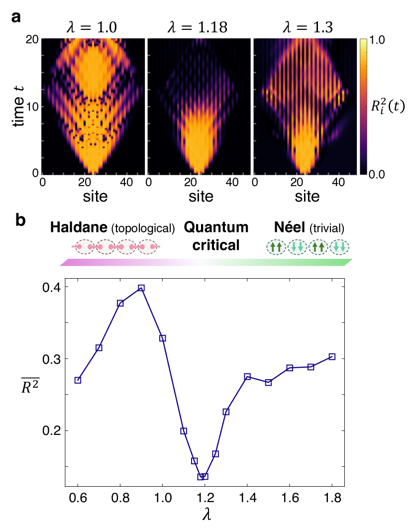
Figure 4: Probing the topological quantum phase transition in the spin-1 XXZ model using the QRP. a Spatiotemporal representation of the estimation performance $R_{i}^{2}(t)$ employing $\langle S^{z}_{i}(t)\rangle$ for a system with $N+1=49$ sites. The time evolution is calculated with a bond dimension of $\chi=128$. b The average $\overline{R^{2}}$ over a subset $(i,t)\in\Lambda\times\{0<t\leq 20\}$, where $\Lambda$ represents the entire system. The upper bar illustrates the phase diagram of $\mathcal{H}(\lambda)$ with schematics composed of virtual $S=1/2$ spins.

In Fig. 4a, we present the estimation performance $R^{2}_{i}(t)$ under the Hamiltonian $\mathcal{H}$ for three different anisotropies: $\lambda=1.0$ in the Haldane phase, $\lambda=1.3$ in the Néel phase, and $\lambda=1.18$ at the vicinity of the quantum critical point. The spread of nonzero $R^{2}_{i}(t)$ values indicates that the operator $S_{i}^{z}(t)$ is reflective of the local quantum quench at various spatiotemporal points, similar to what is observed in $S=1/2$ spin systems. Notably, following an initial transient period, $R^{2}_{i}(t)$ displays a distinct stripy distribution in the Néel phase. This pattern is attributed to the existence of two distinct magnon modes, each originating from one of the two sublattices characteristic of the Néel state. The central quantum manipulation selectively influences one of these modes more than the other. Corresponding to the affected magnon mode, nonzero $R^{2}_{i}(t)$ are observed for sites of the same parity as the central site. In contrast, in the Haldane phase, the local manipulation triggers the reformation of singlet pairs, originating from the central site and diffusively spreading throughout the system. Presumably reflecting the underlying topological nature of the system, this process leads to a distribution of $R^{2}_{i}(t)$ that is markedly different from the stripy pattern seen in the Néel phase. Around the critical point, a notable trend is observed in the values of $R^{2}_{i}(t)$, showing a progressive decline towards zero. This tendency is expected to be a universal feature in quantum critical points, where the impact of local quench operation on local spin dynamics become diminished due to the enhanced fluctuations (Figs. 2a and 3a).

Figure 4b present the mean value $\overline{R^{2}}$, which effectively distinguishes these three distinct distributions of $R^{2}_{i}(t)$. The mean value is computed using $R^{2}_{i}(t)$ values for the entire system within the time interval $0<t\leq 20$, due to the apparent absence of edge reflection effects in Fig. 4a. A key observation in Fig. 4b is the pronounced dip at approximately $\lambda\simeq\lambda_{c}$. This dip serves as a marker for the quantum critical point with strong fluctuations, clearly delineating the boundary between the topological Haldane phase and the trivial Néel phase. Consequently, even in the absence of local order parameters in the Haldane phase, the response of the local spin to the local quantum quench, statistically captured by $R^{2}_{i}(t)$, proves to be a potent indicator for detecting the topological quantum phase transition.

DISCUSSION

To summarize, we have proposed the QRP as an universal tool for identifying the quantum phase transitions in a variety of quantum systems, including integrable, nonintegrable, and topological systems, in a manner similar to the pump-probe paradigm. Here, the parametrized local quantum quench, acting as the “pump”, injects random disturbance into the dynamics. The estimation performance of this random input parameter, through the linear transformation of the single-site operator, serves as the “probe”. This pump-probe-like process informationally discerns the underlying relationship between the local quench and the resultant dynamics of operators. Through the lens of the QRP, we have observed that the influences of the local quench operation are different depending on the intrinsic nature of the quantum phases, manifesting in phenomena such as low-energy excitations, modulation of phase and amplitude of quasiparticles, selective impact on antiferromagnetic magnons, and reformation of topological singlet pairs; these phenomena are challenging to selectively probe through global quenches. At the quantum critical points, the introduced disturbance becomes subordinate to the maximally enhanced intrinsic fluctuations. A noticeable decline in the estimation performance at these points serves as a universal marker for the transition between distinct quantum phases.

Our investigations have focused on 1D quantum spin systems; however, the QRP methodology is applicable to a broader range of quantum systems in more than one dimension as well. Indeed, the conformal field theories governing quantum phase transitions in two and higher-dimensional systems exhibit significant differences from their 1D counterparts [47]. These differences manifest themselves as changes in nature of excitations, intrinsic dynamics, and critical behaviors near quantum critical points, all of which would be detectable through the QRP. Moreover, geometric frustrations in high-dimensional quantum spin systems, coupled with the inherent quantum fluctuations, give rise to a plethora of topological quantum phase transitions in a variety of systems. Especially in certain systems, such transitions are associated with the emergence of anyons, which have promising potential for applications in topological quantum computing [48]. The examination of how anyons respond to local quantum operations through the QRP holds significant importance in light of the aforementioned applications. We leave the high-dimensional applications of the QRP for future investigations.

The QRP framework offers significant advantages over other dynamical detection methodologies for quantum phase transitions. Its unique approach, which leverages only the dynamics of a single-site spin operator, is a marked departure in simplicity from other protocols, such as the utilization of out-of-time-ordered correlators, which requires measurements of operator correlations across various spatial and temporal points. Furthermore, the QRP demonstrates the capability to distinguish quantum phases only from the initial stages of dynamics, highlighting its practicality even when coherence time constraints are considered. We note that, in experiments involving ultracold atoms, the preparation of ground states located distant from phase boundaries is relatively straightforward [11, 49, 50, 51]. This ease of state preparation would remain unhindered by the incorporation of local magnetic fields for the local quench operation, making the initial state configuration in Eq. (1) plausible for experimental implementation. Specifically, for models such as the transverse-field Ising and the ANNNI models, our approach adopts fully polarized initial conditions as described in Eq. (7), which can be realized with remarkable fidelity [52, 20, 6]. These advantageous characteristics of the QRP accentuate its prominence as an effective tool for investigating quantum many-body systems.

Finally, let us remark on the design flexibility of the QRP. A fundamental advantage of employing local quantum quenches, in contrast to global ones, lies in their capability to access and elucidate quantum phenomena induced by local operations, such as specific classes of excitations. Indeed, the concept of excitation in quantum systems is intrinsically linked to the relative relationship between local manipulations and initial states; thus, identical local quench operations can lead to varying outcomes based on the differences in the initial states. When one possesses prior knowledge regarding the physics of the targeted system, especially for discerning partially understood phenomena, the optimal selections for the initial state, local quantum quench, and read-out operators in the QRP become intuitively evident, as demonstrated in our research. In contrast, the true value of the QRP framework becomes markedly pronounced in the exploration of completely unknown quantum systems. Here, the underlying physics remains undisclosed, rendering the interpretation of the complex dynamics observed a formidable task. Our QRP introduces a systematic methodology to address this complexity, categorizing operators by meticulously investigating their dependence on various local operations through a scan of the aforementioned conditions of the QRP. Consequently, we believe that the QRP presents a promising methodology for eliciting novel insights into a broad spectrum of exotic quantum many-body phenomena, extending beyond quantum phase transitions.

METHODS

State evaluation and time evolution

To construct the initial state $|\Psi_{k}^{\mathrm{in}}\rangle$ defined in Eq. (1), we employ the density matrix renormalization group (DMRG) method [53, 54, 55]. For this purpose, we formulate an $(N+1)$-site Hamiltonian $\mathcal{H}_{\mathrm{DMRG}}$ that is specifically designed to have $|\Psi_{k}^{\mathrm{in}}\rangle$ as its ground state. The $N$-site initial Hamiltonian $\mathcal{H}_{I}$ is incorporated into ${\mathcal{H}_{\mathrm{DMRG}}}$, with careful attention to maintaining the independence of the site $N/2+1$, where the magnetic field is applied on inputting $s_{k}$. This is achieved by matching sites from $N/2+1$ to $N$ of $\mathcal{H}_{I}$ with sites from $N/2+2$ to $N+1$ of $\mathcal{H}_{\mathrm{DMRG}}$, while keeping site $1$ to $N/2$ in both Hamiltonians are correspondingly aligned. The local magnetic field $\bm{h}$, which depends on the input $s_{k}$ as specified in Eq. (3) for the spin-$1/2$ case, is applied to the site at $N/2+1$ of ${\mathcal{H}_{\mathrm{DMRG}}}$. The initial state is then obtained as the ground state of $\mathcal{H}_{\mathrm{DMRG}}$ using the DMRG method, expressed as a matrix product state with a bond dimension $\chi$. For the time-evolution $e^{-i\mathcal{H}t}|\Psi_{k}^{\mathrm{in}}\rangle$, we employ the time-dependent variational principle [56, 57, 58] with a bond dimension $\chi$ and a time step $\Delta t=0.005$. The tensor network calculations are implemented using the Julia version of the ITensor library [59, 60].

Statistical treatment in the QRP

From a uniform distribution $[0,1]$, a set of $256$ input values $\{s_{k}\}$ is sampled. Each input $s_{k}$ produces a distinct initial state $|\Psi_{k}^{\mathrm{in}}\rangle$, and the dynamics of operator $\langle O_{i}(t)\rangle_{k}$ is subsequently calculated. Among them, $l^{\mathrm{tr}}=128$ instances are designated for training, while the remaining $l^{\mathrm{ts}}=128$ instances are reserved for testing. The linear transformation is represented using a 2D vector $\bm{x}_{i,k}(t)=\left(\langle O_{i}(t)\rangle_{k},1\right)$ and expressed as $y_{i,k}(t)=\bm{x}_{i,k}(t)\bm{w}_{i}(t)$, with the weight vector $\bm{w}_{i}(t)=(w_{i,O}(t),w_{i,c}(t))^{\top}$.

In the training phase, an ($l^{\mathrm{tr}}\times 2$)-dimensional matrix $X_{i}^{\mathrm{tr}}(t)=\{\bm{x}_{i,k}(t)\}_{k=1}^{l^{\mathrm{tr}}}$ is constructed by summing up the observed dynamics. The output, represented as an $l^{\mathrm{tr}}$-dimensional vector $\bm{y}_{i}^{\mathrm{tr}}(t)=\{y_{i,k}\}_{k=1}^{l^{\mathrm{tr}}}$, is calculated as $\bm{y}_{i}^{\mathrm{tr}}(t)=X^{\mathrm{ts}}_{i}(t)\bm{w}_{i}(t)$. The weight vector is trained to closely match the output $\bm{y}_{i}^{\mathrm{tr}}(t)$ with the original input ${\bm{{s}}}^{\mathrm{tr}}=\{s_{k}\}_{k=1}^{l^{\mathrm{tr}}}$. The optimal solution, which minimizes the least squared error between these vectors, is given by

$$\bm{w}_{i}(t)={{X}_{i}}(t)^{+}{\bm{{s}}}^{\mathrm{tr}},$$ (10)

where ${{X}_{i}^{\mathrm{tr}}}(t)^{+}$ denotes the Moore-Penrose pseudoinverse-matrix of ${{X}_{i}^{\mathrm{tr}}}(t)$.

In the testing phase, an ($l^{\mathrm{ts}}\times 2$)-dimensional matrix $X_{i}^{\mathrm{ts}}(t)=\{\bm{x}_{i,k}(t)\}_{k=l^{\mathrm{tr}}+1}^{l^{\mathrm{tr}}+l^{\mathrm{ts}}}$ is similarly composed, yielding the output $\bm{y}_{i}^{\mathrm{ts}}(t)=X_{i}^{\mathrm{ts}}(t)\bm{w}_{i}(t)$ using the trained weights. The estimation performance is assessed by comparing this testing output with the corresponding input ${\bm{{s}}}^{\mathrm{ts}}=\{s_{k}\}_{k=l^{\mathrm{tr}}+1}^{l^{\mathrm{tr}}+l^{\mathrm{ts}}}$ using the determination coefficient

$$R^{2}_{i}(t)=\frac{\mathrm{cov}^{2}(\bm{y}^{\mathrm{ts}}_{i}(t),{\bm{{s}}}^{\mathrm{ts}})}{\sigma^{2}(\bm{y}^{\mathrm{ts}}_{i}(t))\sigma^{2}({\bm{{s}}}^{\mathrm{ts}})}.$$ (11)

Here, $\mathrm{cov}$ and $\sigma^{2}$ denote covariance and variance, respectively. The coefficient $R^{2}_{i}(t)$ statistically assesses the extent to which $O_{i}(t)$ is influenced by the local quantum quench parameterized by $s_{k}$. We have verified that a smaller dataset with $l^{\mathrm{tr}}=100$ and $l^{\mathrm{ts}}=100$ produces quantitatively similar results.

DATA AVAILABILITY

The data that support the findings of this study are available from the corresponding author upon reasonable request.

CODE AVAILABILITY

The simulation codes used in this study are available from the corresponding author upon reasonable request.

AUTHOR CONTRIBUTIONS

K.K. and Y.M. conceived the project. K.K performed the detailed calculations and analyzed the results under the supervision of Y.M. All authors contributed to writing the paper.

COMPETING INTERESTS

The authors have no conflicts of interest directly relevant to the content of this article.

Supplementary Information for

Quantum reservoir probing of quantum phase transitions
Kaito Kobayashi^∗ and Yukitoshi Motome

Department of Applied Physics, the University of Tokyo, Tokyo 113-8656, Japan

(Dated: )

^∗Corresponding author. E-mail: kaito-kobayashi92@g.ecc.u-tokyo.ac.jp

Supplementary Note 1: Average of the estimation performance over various subsets of spatiotemporal indices

In the main text, we have demonstrated the efficacy of the quantum reservoir probing (QRP) in identifying quantum phase transitions through a statistical analysis of the response to a local quantum quench, as described by the estimation performance $R^{2}_{i}(t)$ in Eq. (5) in the main text. Figures 2d and 3b in the main text illustrate the signatures of quantum phase transitions and quantum critical points, utilizing the mean value of $R^{2}_{i}(t)$, which is calculated over selected spatiotemporal indices $(i,t)$ to minimize extraneous effects from the edges of the systems. Particularly, in the case of the transverse-field Ising model in Fig. 2d, we have presented the field dependence of the mean estimation performance $\overline{R^{2}}$, which is obtained by averaging $R^{2}_{i}(t)$ for indices $(i,t)\in\Lambda\times\{0<t\leq 10\}$, where $\Lambda$ encompasses the central $11$ sites. Similarly for the ANNNI model in Fig. 3b, we have exhibited $\overline{R^{2}}$ defined over $(i,t)$ drawn from the set $\Lambda\times\{0<t\leq 15\}$, where $\Lambda$ also contains central $11$ sites. It is imperative to note that the quantum phases manifest distinguishable characteristics in the spatiotemporal distribution patterns of $R^{2}_{i}(t)$ in Figs. 2a and 3a in the main text, and $\overline{R^{2}}$ serves as an ancillary tool to further clarify these characteristics. In this Supplementary Note, we present $\overline{R^{2}}$ defined for various subsets of spatiotemporal indices $(i,t)$, thus demonstrating the robustness of the QRP in detecting quantum phase transitions independent of the employed spatiotemporal subset.

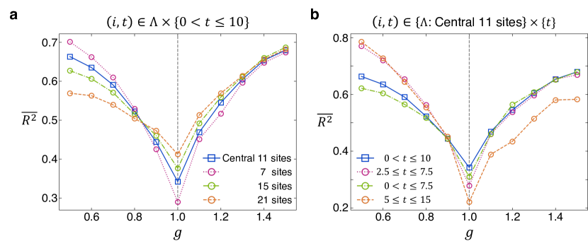
Figure S1: Average of the estimation performance in the transverse-field Ising model over various subsets of spatiotemporal indices. a The average $\overline{R^{2}}$ over subsets $(i,t)\in\Lambda\times\{0<t\leq 10\}$, where $\Lambda$ encompasses the central 11 sites (blue), central 7 sites (pink), central 15 sites (green), and central 21 sites (orange). b The average $\overline{R^{2}}$ over a subsets $(i,t)\in\Lambda\times\{t\}$, where $\Lambda$ encompasses the central 11 sites. The time window is $0<t\leq 10$ (blue), $2.5<t\leq 7.5$ (pink), $0<t\leq 7.5$ (green), and $5\leq t\leq 15$ (orange). The system size is $N+1=49$ in both (a) and (b).

Figure S1 displays the average $\overline{R^{2}}$ in the transverse-field Ising model as a function of the field $g$ in the evolution Hamiltonian $\mathcal{H}(g)$. In Fig. S1a, we show $\overline{R^{2}}$ computed over various spatial index sets $\Lambda$, while the temporal index range is held constant at $\{0<t\leq 10\}$. Conversely, in Fig. S1b, we present $\overline{R^{2}}$ calculated over fixed sets $\Lambda$, which encompass the central eleven sites, while changing the temporal index range. While each curve corresponding to the subset $\{(i,t)\}$ exhibits distinct shapes, the qualitative characteristics are consistent: $\overline{R^{2}}$ decreases as it approaches $g=1.0$, reaches a minimum at $g_{c}$ due to the strong fluctuations, and subsequently rises with further increasing $g$. These patterns robustly indicate the occurrence of a quantum phase transition, with the quantum critical point at $g_{c}$ demarcating the transition between the ferromagnetically ordered phase and the quantum disordered phase.

Figure S2 demonstrates the averaged estimation performance in the ANNNI model as a function of the field strength. Figure S2a illustrates $\overline{R^{2}}$ calculated over various spatial index sets $\Lambda$ with the temporal index range consistently set at $\{0<t\leq 15\}$. In addition, Fig. S2b illustrates $\overline{R^{2}}$ calculated over a fixed spacial indices set $\Lambda$ that includes the central eleven sites, while varying the temporal index range. Similar to the observations in the transverse-field Ising model, the qualitative behaviors of $\overline{R^{2}}$ in the ANNNI model remain consistent across different subsets $\{(i,t)\}$, with all results corroborating the occurrence of a quantum phase transition around $g_{c}\simeq 1.6$. However, a notable feature in the ANNNI model is the broader shape of the dip in $\overline{R^{2}}$ near the quantum critical point, which leads to variations in the identified field strength at which $\overline{R^{2}}$ reaches its minimum depending on the specific subset employed. Nevertheless, it is anticipated that this variance would decrease as the system size increases. A larger system would reduce the influence of edge effects, which are the principal cause of the subset $\{(i,t)\}$ dependency in $\overline{R^{2}}$. Consequently, in a larger system, the quantum critical point is expected to be identified with greater precision and clarity.

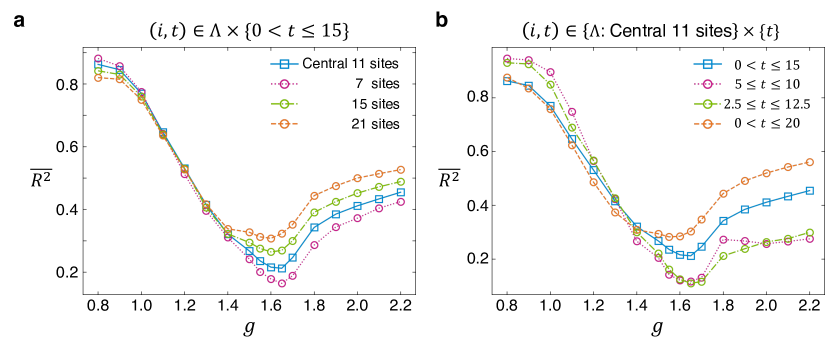
Figure S2: Average of the estimation performance in the ANNNI model over various subsets of spatiotemporal indices. a The average $\overline{R^{2}}$ over subsets $(i,t)\in\Lambda\times\{0<t\leq 15\}$, where $\Lambda$ encompasses the central 11 sites (skyblue), central 7 sites (pink), central 15 sites (green), and central 21 sites (orange). b The average $\overline{R^{2}}$ over subsets $(i,t)\in\Lambda\times\{t\}$, where $\Lambda$ encompasses the central 11 sites. The time window is $0<t\leq 15$ (skyblue), $5\leq t\leq 10$ (pink), $2.5\leq t\leq 12.5$ (green), and $0<t\leq 20$ (orange). The system size is $N+1=49$ in both (a) and (b).

References

- [1] Sachdev, S. Quantum Phase Transitions (Cambridge University Press, 2011), 2 edn.
- [2] Zinn-Justin, J. Quantum Field Theory and Critical Phenomena: Fifth Edition (Oxford University Press, 2021).
- [3] Heyl, M., Pollmann, F. & Dóra, B. Detecting equilibrium and dynamical quantum phase transitions in ising chains via out-of-time-ordered correlators. Phys. Rev. Lett. 121, 016801 (2018).
- [4] Dağ, C. B., Sun, K. & Duan, L.-M. Detection of quantum phases via out-of-time-order correlators. Phys. Rev. Lett. 123, 140602 (2019).
- [5] Wei, B.-B., Sun, G. & Hwang, M.-J. Dynamical scaling laws of out-of-time-ordered correlators. Phys. Rev. B 100, 195107 (2019).
- [6] Nie, X. et al. Experimental observation of equilibrium and dynamical quantum phase transitions via out-of-time-ordered correlators. Phys. Rev. Lett. 124, 250601 (2020).
- [7] Bin, Q., Wan, L.-L., Nori, F., Wu, Y. & Lü, X.-Y. Out-of-time-order correlation as a witness for topological phase transitions. Phys. Rev. B 107, L020202 (2023).
- [8] Titum, P., Iosue, J. T., Garrison, J. R., Gorshkov, A. V. & Gong, Z.-X. Probing ground-state phase transitions through quench dynamics. Phys. Rev. Lett. 123, 115701 (2019).
- [9] Haldar, A. et al. Signatures of quantum phase transitions after quenches in quantum chaotic one-dimensional systems. Phys. Rev. X 11, 031062 (2021).
- [10] Robertson, J. H., Senese, R. & Essler, F. H. L. A simple theory for quantum quenches in the ANNNI model. SciPost Phys. 15, 032 (2023).
- [11] Leibfried, D., Blatt, R., Monroe, C. & Wineland, D. Quantum dynamics of single trapped ions. Rev. Mod. Phys. 75, 281–324 (2003).
- [12] Blatt, R. & Roos, C. F. Quantum simulations with trapped ions. Nature Phys. 8, 277–284 (2012).
- [13] Richerme, P. et al. Non-local propagation of correlations in quantum systems with long-range interactions. Nature 511, 198–201 (2014).
- [14] Neyenhuis, B. et al. Observation of prethermalization in long-range interacting spin chains. Sci. Adv. 3, e1700672 (2017).
- [15] Kinoshita, T., Wenger, T. & Weiss, D. S. A quantum newton’s cradle. Nature 440, 900–903 (2006).
- [16] Bloch, I., Dalibard, J. & Zwerger, W. Many-body physics with ultracold gases. Rev. Mod. Phys. 80, 885–964 (2008).
- [17] Bloch, I., Dalibard, J. & Nascimbène, S. Quantum simulations with ultracold quantum gases. Nature Phys. 8, 267–276 (2012).
- [18] Schreiber, M. et al. Observation of many-body localization of interacting fermions in a quasirandom optical lattice. Science 349, 842–845 (2015).
- [19] Zeiher, J. et al. Many-body interferometry of a rydberg-dressed spin lattice. Nature Phys. 12, 1095–1099 (2016).
- [20] Zeiher, J. et al. Coherent many-body spin dynamics in a long-range interacting ising chain. Phys. Rev. X 7, 041063 (2017).
- [21] Bernien, H. et al. Probing many-body dynamics on a 51-atom quantum simulator. Nature 551, 579–584 (2017).
- [22] Guardado-Sanchez, E. et al. Probing the quench dynamics of antiferromagnetic correlations in a 2d quantum ising spin system. Phys. Rev. X 8, 021069 (2018).
- [23] Choi, S. et al. Observation of discrete time-crystalline order in a disordered dipolar many-body system. Nature 543, 221–225 (2017).
- [24] Villa, L., Despres, J., Thomson, S. J. & Sanchez-Palencia, L. Local quench spectroscopy of many-body quantum systems. Phys. Rev. A 102, 033337 (2020).
- [25] Villa, L., Thomson, S. J. & Sanchez-Palencia, L. Finding the phase diagram of strongly correlated disordered bosons using quantum quenches. Phys. Rev. A 104, 023323 (2021).
- [26] Schneider, J. T., Despres, J., Thomson, S. J., Tagliacozzo, L. & Sanchez-Palencia, L. Spreading of correlations and entanglement in the long-range transverse ising chain. Phys. Rev. Res. 3, L012022 (2021).
- [27] Kobayashi, K. & Motome, Y. Quantum reservoir probing of quantum information scrambling. arXiv preprint arXiv:2308.00898 (2023).
- [28] Jaeger, H. & Haas, H. Harnessing nonlinearity: Predicting chaotic systems and saving energy in wireless communication. Science 304, 78–80 (2004).
- [29] Fujii, K. & Nakajima, K. Harnessing disordered-ensemble quantum dynamics for machine learning. Phys. Rev. Appl. 8, 024030 (2017).
- [30] Tanaka, G. et al. Recent advances in physical reservoir computing: A review. Neural Networks 115, 100–123 (2019).
- [31] Kobayashi, K. & Motome, Y. Thermally-robust spatiotemporal parallel reservoir computing by frequency filtering in frustrated magnets. Sci. Rep. 13, 15123 (2023).
- [32] Coldea, R. et al. Quantum criticality in an ising chain: Experimental evidence for emergent e¡sub¿8¡/sub¿ symmetry. Science 327, 177–180 (2010).
- [33] Selke, W. The annni model ― theoretical analysis and experimental application. Phys. Rep. 170, 213–264 (1988).
- [34] Beccaria, M., Campostrini, M. & Feo, A. Density-matrix renormalization-group study of the disorder line in the quantum axial next-nearest-neighbor ising model. Phys. Rev. B 73, 052402 (2006).
- [35] Suzuki, S., Inoue, J.-i. & Chakrabarti, B. K. Quantum Ising Phases and Transitions in Transverse Ising Models (Springer, Heidelberg, 2013).
- [36] Karrasch, C. & Schuricht, D. Dynamical phase transitions after quenches in nonintegrable models. Phys. Rev. B 87, 195104 (2013).
- [37] Haldane, F. D. M. Continuum dynamics of the 1-d heisenberg antiferromagnet: Identification with the o(3) nonlinear sigma model. Phys. Lett. A 93, 464–468 (1983).
- [38] Haldane, F. D. M. Nonlinear field theory of large-spin heisenberg antiferromagnets: Semiclassically quantized solitons of the one-dimensional easy-axis néel state. Phys. Rev. Lett. 50, 1153–1156 (1983).
- [39] Botet, R. & Jullien, R. Ground-state properties of a spin-1 antiferromagnetic chain. Phys. Rev. B 27, 613–615 (1983).
- [40] Botet, R., Jullien, R. & Kolb, M. Finite-size-scaling study of the spin-1 heisenberg-ising chain with uniaxial anisotropy. Phys. Rev. B 28, 3914–3921 (1983).
- [41] Sakai, T. & Takahashi, M. Finite-size scaling study of s=1 xxz spin chain. J. Phys. Soc. Jpn. 59, 2688–2693 (1990).
- [42] den Nijs, M. & Rommelse, K. Preroughening transitions in crystal surfaces and valence-bond phases in quantum spin chains. Phys. Rev. B 40, 4709–4734 (1989).
- [43] Pollmann, F., Turner, A. M., Berg, E. & Oshikawa, M. Entanglement spectrum of a topological phase in one dimension. Phys. Rev. B 81, 064439 (2010).
- [44] Pollmann, F., Berg, E., Turner, A. M. & Oshikawa, M. Symmetry protection of topological phases in one-dimensional quantum spin systems. Phys. Rev. B 85, 075125 (2012).
- [45] Nomura, K. Spin-correlation functions of the s=1 heisenberg-ising chain by the large-cluster-decomposition monte carlo method. Phys. Rev. B 40, 9142–9146 (1989).
- [46] Chen, W., Hida, K. & Sanctuary, B. C. Ground-state phase diagram of chains with uniaxial single-ion-type anisotropy. Phys. Rev. B 67, 104401 (2003).
- [47] Di Francesco, P., Mathieu, P. & Sénéchal, D. Conformal field theory. Graduate Texts in Contemporary Physics (Springer, Germany, 1997).
- [48] Kitaev, A. Anyons in an exactly solved model and beyond. Ann. Phys. 321, 2–111 (2006). January Special Issue.
- [49] Kim, K. et al. Quantum simulation of frustrated ising spins with trapped ions. Nature 465, 590–593 (2010).
- [50] Georgescu, I. M., Ashhab, S. & Nori, F. Quantum simulation. Rev. Mod. Phys. 86, 153–185 (2014).
- [51] Sompet, P. et al. Realizing the symmetry-protected haldane phase in fermi–hubbard ladders. Nature 606, 484–488 (2022).
- [52] Lanyon, B. P. et al. Universal digital quantum simulation with trapped ions. Science 334, 57–61 (2011).
- [53] White, S. R. Density matrix formulation for quantum renormalization groups. Phys. Rev. Lett. 69, 2863–2866 (1992).
- [54] White, S. R. Density-matrix algorithms for quantum renormalization groups. Phys. Rev. B 48, 10345–10356 (1993).
- [55] Schollwöck, U. The density-matrix renormalization group. Rev. Mod. Phys. 77, 259–315 (2005).
- [56] Haegeman, J. et al. Time-dependent variational principle for quantum lattices. Phys. Rev. Lett. 107, 070601 (2011).
- [57] Haegeman, J., Lubich, C., Oseledets, I., Vandereycken, B. & Verstraete, F. Unifying time evolution and optimization with matrix product states. Phys. Rev. B 94, 165116 (2016).
- [58] Yang, M. & White, S. R. Time-dependent variational principle with ancillary krylov subspace. Phys. Rev. B 102, 094315 (2020).
- [59] Fishman, M., White, S. R. & Stoudenmire, E. M. The ITensor Software Library for Tensor Network Calculations. SciPost Phys. Codebases 4 (2022).
- [60] Fishman, M., White, S. R. & Stoudenmire, E. M. Codebase release 0.3 for ITensor. SciPost Phys. Codebases 4–r0.3 (2022).
ACKNOWLEDGEMENTS
This research was supported by a Grant-in-Aid for Scientific Research on Innovative Areas “Quantum Liquid Crystals” (KAKENHI Grant No. JP19H05825) from JSPS of Japan and JST CREST (Nos. JP-MJCR18T2). K. K. was supported by the Program for Leading Graduate Schools (MERIT-WINGS). The computation in this work has been done using the facilities of the Supercomputer Center, the Institute for Solid State Physics, the University of Tokyo.