longtable Ginwidth=,height=,keepaspectratio

CodPy: a Python library for numerics,
machine learning, and statistics

Chapter 1 Introduction

1.1 Main objective

This monograph offers an introduction to a collection of numerical algorithms implemented in the library CodPy (an acronym that stands for the Curse Of Dimensionality in PYthon), which has found widespread applications across various areas, including machine learning, statistics, and computational physics. We develop here a strategy based on the theory of reproducing kernel Hilbert spaces (RKHS) and the theory of optimal transport. Initially designed for mathematical finance, this library has since been enhanced and broadened to be applicable to problems arising in engineering and industry.

In order to present the general principles and techniques employed in CodPy and its applications, we have structured this monograph into two main parts. In Chapters 2 to 5, we focus on the fundamental principles of kernel-based representations of data and solutions, aso that the presentation therein is supplemented with illustrative examples only. Next, in Chapters 6 to 9 we discuss the application of these principles to many classes of concrete problems, spanning from the numerical approximation of partial differential equations to (supervised, unsupervised) machine learning, extending to generative methods with a focus on stochastic aspects.

We have aimed to make this monograph as self-contained as possible, and primarily targeted towards engineers. We have intentionally omitted theoretical aspects of functional analysis and statistics which can be found elsewhere in the existing literature, and we chose to emphasize the operational applications of kernel-based methods. We solely assume that the reader has a basic knowledge of linear algebra, probability theory, and differential calculus. Our core objective is to provide a framework for applications, enabling the reader to apply the proposed techniques in CodPy.

Obviously, this text cannot cover all possible directions on the vast subject that we touch upon here. Yet, we hope that this monograph can put in light the particularly robust strengths of kernel methods, and contribute to bridge, on the one hand, basic ideas of functional analysis and optimal transport theory and, on the other hand, a robust framework for machine learning and related topics. With this emphasis in mind, we have designed here novel numerical strategies, while demonstrating the versatility and competitiveness of the CodPy methods for dealing with machine learning problems, among others.

1.2 Outline of this monograph

More specifically, this monograph provides a comprehensive study of kernel-based machine learning methods and their application across a diverse range of topics within mathematics, finance, and engineering, and is organized as follows.

• Chapter 2 establishes the foundation for our discussion by introducing the terminology and notation used throughout this monograph. It offers a succinct overview of machine learning techniques and existing libraries, primarily focusing on the nature of numerical algorithms in machine learning, and the notions of loss functions and performance indicators (also referred to as error estimates). Additionally, a brief discussion on currently available libraries is included here.

• Chapter 3 presents the core aspects of the kernel techniques, starting from the basic concepts of reproducing kernels, moving on to kernel engineering, and then discussing interpolation and extrapolation (or projection) operators. This chapter also presents the notion of kernel-discrepancy error and kernel-based norms, paving the way to design effective performance indicators which allow us to decide about the relevance of projection operators in any specific application.

• In Chapter 4, we define and investigae the properties of kernel-based differential operators in greater depth. These operators play a key role in the discretization of partial differential equations, making them particularly useful in physics and engineering. Interestingly, they also find major applications in machine learning, especially in order to predict deterministic, non-stochastic functions of the unknown variables. We also discuss here error estimates and propose a novel clustering method that bridges kernel methods and transport theory together.

• Chapter 5 extends our investigation of the interconnection between transport theory and kernel-discrepancy errors. This relationship paves the way for the development of high-performing generative methods, as well as addressing numerical challenges such as numerical simulations of joint probabilities and computations of optimal transport mappings.

• Chapter 6 showcases the efficiency of the kernel techniques in solving partial differential equations on unstructured meshes. We consider a range of academic problems, starting from the Laplace equation to fluid dynamics equations together with the Lagrangian methods employed in particle, mesh-free methods. This chapter also highlights the power of the proposed framework in enhancing the convergence of Monte-Carlo methods, and briefly touches on automatic differentiation —an essential yet intrusive tool.

• Chapters 7 and 8 focus on supervised and unsupervised machine learning. We compare our framework against various machine learning methods, benchmarking across multiple scenarios and performance indicators, while analyzing their suitability for several different types of learning problems.

• Finally, Chapter 9 explores generative methods with a focus on their applications in mathematical finance. We explore areas such as time-series analysis and prediction, as well as their applications in financial derivative portfolios, investment strategies, and risk management strategies.

In our endeavor to make this monograph more accessible and user-friendly, we have integrated Python, R, and LaTeX codes together, and developed Jupyter notebooks, all built on a high-performance C++ core. The CodPy Library provides a robust and versatile toolset for tackling a wide range of practical challenges. This open-source code (soon made available for download) aims to help the readers to learn and experiment with our code, while also offering a foundation for the techniques that can be tailored to specific applications. Additionally, this is a dynamical project, and we expect this monograph to be updated as new versions become available and to help validate new releases of the CodPy Library.

By presenting a fresh perspective on kernel-based methods and offering a broad overview of their applications, this monograph should stand as a resource for researchers, students, and professionals in the fields of scientific computation, statistics, mathematical finance, and engineering sciences.

1.3 References

There is a vast literature available on kernel methods and reproducing kernel Hilbert spaces which we do not attempt to review here. Our focus is on providing a practical framework for the application of such methods. However, for the reader interested in a comprehensive review of the theory we refer to several textbooks and research articles such as Berlinet and Thomas-Agnan [3] and Fasshauer [11],[12],[13].

Our kernel-based meshfree algorithms presented in Chapters 3 to 5 are based on the research papers [30],[31],[32],[33],[34]. Earlier versions of this material can also be found also in unpublished notes [35]–[40].

For additional information on meshfree methods in fluid dynamics and material science, the reader is referred to the following works: [2],[4],[16],[18],[23], [41],[43],[46],[49],[52],[56],[64].

Chapter 2 Overview of methods of machine learning

2.1 A framework for machine learning

2.1.1 Prediction machine for supervised/unsupervised learning

Machine learning methods can be broadly categorized into two main approaches: unsupervised methods and supervised methods. These methods provide a prediction machine, which can be understood as a system that makes predictions based on input data. In the framework under consideration, a predictor is defined as an extrapolation or interpolation operator, denoted by $\mathcal{P}_{m}$. The class of operators of interest (our notation being explained in the next paragraph) reads

$$f_{z}=\mathcal{P}_{m}\big{(}X,Y=[\,],Z=X,f(X)\big{)}.$$

Using standard Python notation, the empty brackets indicate that the variables $Y$ and $Z$ represent optional input data.

The subscript $m$ is introduced to specify the choice of the method. On the one hand, each method relies on a set of external parameters, or hyperparameters, which should be specified before training. On the other hand, fine-tuning these external parameters can be challenging and error-prone. As a matter of fact, some strategies in the literature even propose using a machine learning approach to determine these parameters. When selecting a method, it is crucial to consider performance indicators before tuning the hyperparameters.

Let us specify our notation, in which $X$, $Y$, and $Y$ can be regarded as matrices (of various dimensions).

• The input data $X,Y,Z,f(X)$ are as follows.

  • The (non-optional) parameter $X\in\mathbb{R}^{N_{x},D}$ is called the training set. This is a matrix where each row represents a data sample of a distribution $\mathbb{X}$ and each column represents a certain feature. The parameter $D$ denotes the total number of features in the dataset.

  • The variable $f(X)\in\mathbb{R}^{N_{x},D_{f}}$ is called the training set values. These are the target values or labels associated with each sample in the training set. The parameter $D_{f}$ is the dimensionality of the target values. There is an important distinction to be made here:

    • Deterministic case, if $f(X)$ is considered as a continuous function of $X$. This book details kernel methods for this case in the two following chapters.

    • Stochastic case, if $f(X)\equiv\mathbb{E}(f\ |\ \mathbb{X})$ is considered as a random variable, conditioned by $X$. Kernel methods for this case are discussed chapter (5.3.2).

  • The variable $Z\in\mathbb{R}^{N_{z},D}$ is the test set. This is a separate set of data samples used to evaluate the model performance on unseen data. If $Z$ is not explicitly provided, it is assumed that $Z=X$ (that is, the test set is then the same as the training set).

  • The variable $Y\in\mathbb{R}^{N_{y},D}$ is called the internal parameter set This set is crucial for defining the predictor $\mathcal{P}_{m}$.

• The output data are as follows.

  • Supervised learning: In this approach, the model is trained using known input-output pairs. The goal is to learn a function that can make predictions for new, unseen inputs. Specifically, given the input function values $f(X)$ the relationship is expressed as

    $$f_{Z}=\mathcal{P}_{m}\Big{(}X,Y=[\,],Z=X,f(X)\Big{)}\simeq f(Z),$$ (2.1.1)

    where $f_{Z}$ represens the predicted values and each $f_{z}\in\mathbb{R}^{N_{z},D}$ is termed a prediction. We distinguish between two cases.

    • feed-backward machine. If the input data $Y$ is not provided (i.e. left empty), then the prediction mechanism described by (2.1.1) falls under the category of feed-backward machines. In this scenario, the method internally determines this set and computes the prediction $f_{z}$.

    • feed-forward machine. Conversely, if $Y$ is explicitly specified as input data, then the prediction mechanism from (2.1.1) is called a feed-forward machine. In this case, the method make use of the set of internal parameters in order to compute the prediction $f_{z}$.

  • Unsupervised learning. In this approach, the model is trained without explicit labels or target values. Instead, the goal is to discover underlying patterns or structures in the data. Specifically, the relationship is expressed as:

    $$f_{z}=\mathcal{P}_{m}(X,Z=X),$$ (2.1.2)

    where the output values $f_{z}\in\mathbb{R}^{N_{z},D}$ are called clusters in the context of the so-called clustering method ( which will be elaborated upon later).

Many other machine learning methods can be described with the notation above. For instance, consider two methods denoted by $m_{1}$ and $m_{2}$. Their composition can be defined and describes a feed-backward machine, which is analogous to the notion of semi-supervised learning in the literature (and also encompasses feed-backward learning machines). Specifically, we write

$$f_{z}=\mathcal{P}_{m_{1}}\Big{(}X,\mathcal{P}_{m_{2}}(X,f(X)),Z,f(X)\Big{)}.$$ (2.1.3)

Here, the term “semi-supervised learning” denotes a learning paradigm where the training dataset comprises both labeled and unlabeled samples. The primary objective is to leverage the unlabeled samples to enhance the model performance on the labeled ones. On the other hand, “feedback learning machines” refer to a specific class of models, in which the output is recursively fed back as input, aiming to refine prediction accuracy via iterations.

We summarize our main notation in Table LABEL:tab:mainnotations. The dimensions of the input data, that is, the integers $D,N_{x},N_{y},N_{z},D_{f}$, are also treated as input parameters. The fundamental distinction between supervised and unsupervised learning lies in the nature of the input data: supervised learning relies on input data for both the features and their associated labels, whereas unsupervised learning only requires input data for the features. We will proceed deeper into this distinction in subsequent sections of this chapter.

Table 2.1: Main parameters for machine learning

$X$	$Y$	$Z$	$f(X)$	$f_{z}$
training set	parameter set	test set	training values	predictions
size $N_{x},D$	size $N_{y},D$	size $N_{z},D_{f}$	size $N_{x},D_{f}$	size $N_{z},Df$

Moreover, from any machine learning method $m$ we can also compute the gradient of a real-valued function $f=f(x_{1},\ldots,x_{D})$ by

$$(\nabla f)_{Z}=(\nabla_{Z}\mathcal{P}_{m})\Big{(}X,Y=[\,],Z=X,f(X)=[\,]\Big{)}\sim\nabla f(Z),$$ (2.1.4)

where the gradient is noted $\nabla=(\partial_{x_{1}},\ldots,\partial_{x_{D}})$, then we say that $m$ is a differentiable learning machine.

2.1.2 Techniques of supervised learning

Supervised learning as in (2.1.1) corresponds to the choice where the function values $f(X)$ is part of the input data:

$$f_{z}=\mathcal{P}_{m}\Big{(}X,Y=[\,],Z=X,f(X)\Big{)}.$$ (2.1.5)

Supervised learning is a technique used to predict or extrapolate the values of a given function on a new set of inputs. In other words, it involves training a model on historical observations of the function $X$ and its corresponding outputs, and then using the trained model to predict the output values on a new set of inputs $Z$.

When considering the terminology of supervised learning, a method is said to be multi-class or multi-output if the function $f$ is vector-valued, meaning $D_{f}\geq 1$ in our notation. It is important to note that while it is possible to combine learning machines to produce multi-class methods, this often comes with a significant computational cost.

Additionally, the input function $f$ can be classified as being discrete, continuous, or mixed. A discrete function has a finite (or countable) number of unique values and is referred to as labels. These labels can always be mapped to an integer range of $[1,\ldots,\#(Ran(f))]$, where $\#(E)$ represents the number of elements or cardinality of a set. A continuous function has an infinite number of possible values, while a mixed function contains both discrete and continuous data.

In our presentation, we distinguish between the following aspects of the subject.

• Typical families of methods: linear models, support vector machines, neural networks,…
  

  

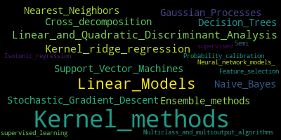
  Figure 2.1: ,

• Examples of particular methods: neural network, Gaussian process,…
  

  

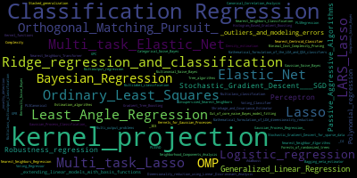
  Figure 2.2: ,

• Open-source machine learning libraries: scikit-learn, TensorFlow,…

2.1.3 Techniques of unsupervised learning

In unsupervised learning, the function values $f(X)$ are not included in the input data, as the operator (2.1.1) reads

$$\mathcal{P}_{m}\Big{(}X,Y=[\,],Z=X\Big{)}.$$ (2.1.6)

In this setting, unsupervised learning can be thought of as an interpolation procedure, where the goal is to extract $N_{y}$ features from a given distribution $X$ that best represents it. A common output of clustering methods is the cluster set, represented by $Y\in\mathbb{R}^{N_{y},D}$.

Supervised and unsupervised learning are connected in several ways.

• Semi-supervised clustering methods use the clusters $y$ as input to a supervised learning machine, which produces a prediction $f_{z}\in\mathbb{R}^{N_{z},D_{f}}$; see (2.1.3).

• In unsupervised clustering methods, a prediction $f_{z}\in\mathbb{R}^{N_{z}}$ can also be made. This prediction assigns each point $z^{i}$ of the test set to the cluster set $Y$, resulting in $f_{z}$ as a map $[1,\ldots,N_{z}]\mapsto[1,\ldots,N_{y}]$.

The task of clustering can be performed using various methods, which are described in standard literature. Moreover, different libraries are available which offer clustering methods — Scikit-learn being one of the most popular approaches. The latter provides an impressive list of clustering methods, which are described in the corresponding website. Furthermore, Figure 2.1 provides an illustration of some of these methods.

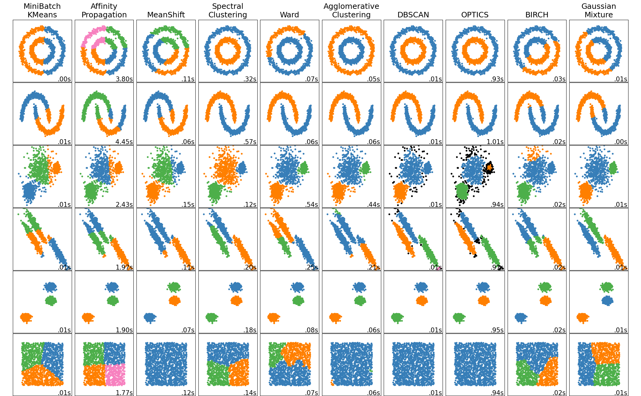
Figure 2.3: Comparison of clustering methods from scikit-learn website

• Each column corresponds to a specific clustering algorithm.

• Each row corresponds to a particular unsupervised clustering problem:

  • Each scatter plot shows the training set $X$ and the test set $Z$, which however coincide for the class of clustering methods under consideration.

  • The color of each point in the scatter plot represents its predicted value $f_{z}$.

2.2 Exploratory data analysis

Preliminaries. Exploratory data analysis (EDA) is a fundamental step in data engineering, as it allows one to gain insights into the structure and statistical properties of a dataset. EDA techniques can help identify correlations, detect outliers, and reveal underlying patterns in the data. In unsupervised learning, EDA can provide an initial estimate of the number of clusters in a dataset or suggests appropriate kernels for regression.

As an example, we demonstrate the use of visualization tools with the Iris flower dataset. The Iris dataset was introduced by the British statistician, eugenicist, and biologist Ronald Fisher in his 1936 paper “The use of multiple measurements in taxonomic problems”. It consists of 150 samples of Iris flowers, with 50 samples from each of three species: Iris setosa, Iris virginica, and Iris versicolor. Each sample has four features: the length and width of the sepals and petals, measured in centimeters.

Non-parametric density estimation. The density of the input data is estimated using a kernel density estimate (KDE). We assume that $(x^{1},x^{2},\dots,x^{N_{X}})$ are independent and identically distributed samples, drawn from an univariate distribution with unknown density $f$ at any given point $x$. Our goal is to estimate the shape of this function $f$, and the kernel density estimator is given by

$$\widehat{f}_{h}(x)={\frac{1}{n}}\sum_{i=1}^{N_{X}}k_{h}(x-x^{i})={\frac{1}{nh}}\sum_{i=1}^{N_{X}}k{\Big{(}}{\frac{x-x^{i}}{h}}{\Big{)}},$$

where $k$ is a kernel (say any non-negative function, at this stage) and $h>0$ is a smoothing parameter called the bandwidth.

KDE is a popular method for estimating the probability density function of a random variable. A key factor in obtaining an accurate density estimate is the choice of the kernel and the smoothing bandwidth. The kernel function determines the shape of the estimated density, while the bandwidth controls the amount of smoothing applied to the data. An appropriate bandwidth for kernel density estimation strikes a balance between over-smoothing, which can obscure important features of the underlying distribution, and under-smoothing, which can result in a noisy estimate that does not accurately capture the true shape of the data. Common kernel functions used in KDE include uniform, triangular, biweight, triweight, Epanechnikov, normal, and others.

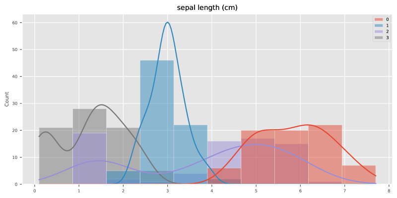
Figure 2.4: Kernel density estimator and histograms of four features

Scatter plot. A scatter plot is a way to visualize data by displaying it as a collection of points. Each point represents a single observation in the dataset, with the value of one variable plotted on the horizontal axis and the value of another variable plotted on the vertical axis. This allows us to see the relationship between the two variables and identify any patterns or trends in the data.

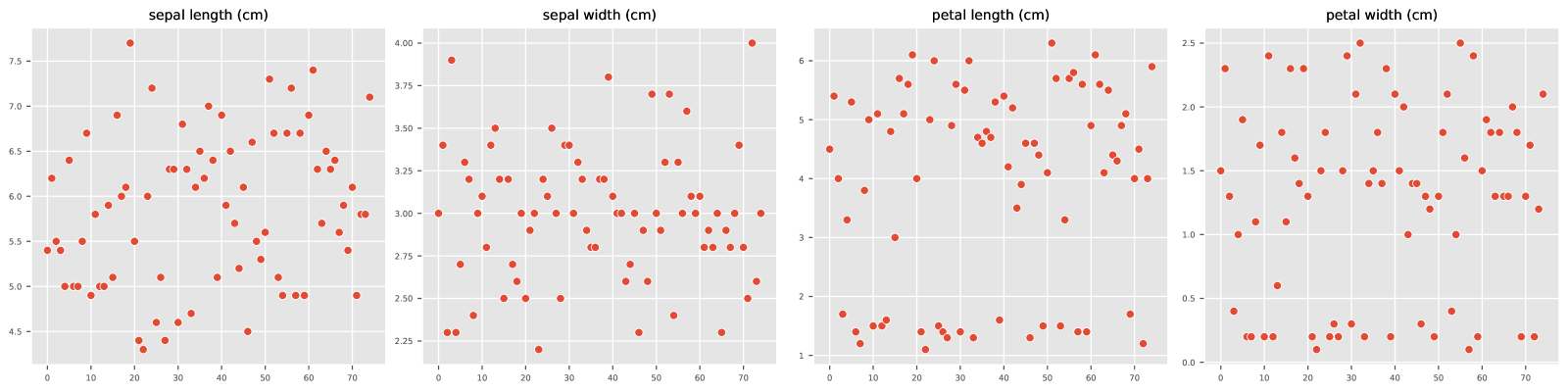
Figure 2.5: Scatter plot

Heat map. The correlation matrix of $n$ random variables $x^{1},\ldots,x^{n}$ is the $n,n$ matrix whose $(i,j)$ entry is $corr(x^{i},x^{j})$. Thus the diagonal entries are all identically unity.

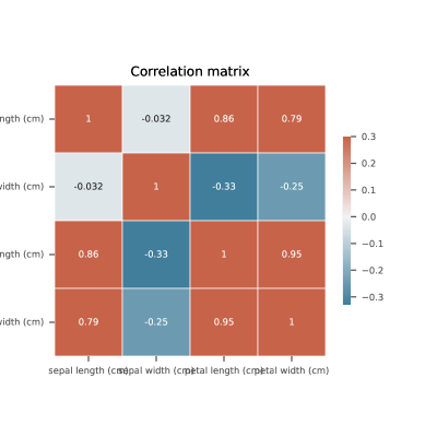
Figure 2.6: Correlation matrix

Summary plot. The summary plot is a visualization tool that displays multiple plots in a grid format. It is used to visualize the relationship between different features of a dataset. In this plot, the density of each feature is displayed on the diagonal. The kernel density estimate plot is displayed on the lower diagonal, which shows the estimated probability density function of the data. The scatter plot is displayed on the upper diagonal, which shows the relationship between two features by plotting them against each other. Overall, the summary plot provides a quick and intuitive way to explore the relationship between different features of a dataset.

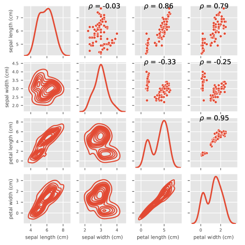
Figure 2.7: Summary plot

2.3 Performance indicators for machine learning

2.3.1 Distances and divergences

f-divergences. The notion of distance between probability distributions has numerous applications in mathematical statistics and information theory, such as hypothesis testing, distribution testing, density estimation, etc. One well-studied family of distances/divergences between probability distributions are the so-called $f-$divergences, which can be classified as follows. Let $f:(0,\infty)\mapsto\mathbb{R}$ be a convex function with $f(1)=0$. Let $P$ and $Q$ be two probability distributions on a discrete measurable space $(\mathcal{X},\mathcal{F})$. If $P$ is absolutely continuous with respect to $Q$, then the $f$-divergence is defined as

$$D_{f}(P||Q)=\mathbb{E}^{Q}\Big{[}f\left(\frac{dP}{dQ}\right)\Big{]}=\sum_{x}Q(x)f\left(\frac{dP(x)}{dQ(x)}\right).$$

We list the following common $f-$divergences.

• Kullback-Leibler (KL) divergence with $f(x)=x\log(x)$.

• Squared Hellinger distance with $f(x)=(1-\sqrt{x})^{2}$. Then the formula of Hellinger distance $\mathcal{H}^{2}(P,Q)$ is given by

$$\mathcal{H}(P,Q)=\frac{1}{\sqrt{2}}||\sqrt{dP}-\sqrt{dQ}||_{2}.$$

Maximum mean discrepancy - or kernel discrepancy. Another popular family of distances are integral probability metrics (IPMs), which include Wasserstein or Kantorovich distances, total variation (TVD) or Kolmogorov distances, and maximum mean discrepancy (MMD) (defined later on in this text).

2.3.2 Indicators for supervised learning

Comparison to ground truth values. A wide range of indicators are available to evaluate the performance of a learning models. Most of these indicators are readily described and implemented in scikit-learn.

We will not discuss here all of the available metrics, but instead we provide an overview of the main metrics we have included in the CodPy library. In the context of semi-supervised methods, if the function $f$ is known in advance, then the predictions of the learning machine $f_{z}$ can be compared with the ground truth values $f(Z)\in\mathbb{R}^{N_{z},D_{f}}$. The following are the primary metrics of interest.

• For labeled functions (i.e., discrete functions), a common indicator is the score, defined as

  $$\frac{1}{N_{z}}\#\{f_{z}^{n}=f(Z)^{n},n=1,\ldots,N_{z}\}.$$ (2.3.1)

  This produces an indicator ranging between 0 and 1, where higher scores indicate better performance.

• For continuous functions (i.e., discrete functions), a common indicator is given by the $\ell^{p}$ norms, defined as

  $$\frac{1}{N_{z}}\|f_{z}-f(Z)\|_{\ell^{p}},\ \quad\quad 1\leq p\leq\infty.$$ (2.3.2)

  The choice $p=2$ is referred to as the root-mean-square error (RMSE).

• As the above indicator is not normalized, a preferred version might be

  $$\frac{\|f_{z}-f(Z)\|_{\ell^{p}}}{\|f_{z}\|_{\ell^{p}}+\|f(Z)\|_{\ell^{p}}},\ \quad\quad 1\leq p\leq\infty.$$ (2.3.3)

  This produces an indicator with values ranging between 0 and 1, where smaller values indicate better performance. It can be interpreted as a percentage of error. In finance, this concept is sometimes referred to as the “basis point indicator’ ’.

Cross validation scores. The cross validation score involves randomly selecting a subset of the training set as the test set, and then calculating a score or RMSE type error analysis for each run. This process is repeated multiple times with different randomly selected test sets, and the results are averaged to give an estimate of the model performance on unseen data. For more information, see the dedicated page on the scikit-learn website.

A confusion matrix is a performance evaluation tool for supervised machine learning algorithms that are used for classification tasks. It is a matrix representation of the number of predicted and actual labels for each class in the data. The matrix has dimensions equal to the number of classes in the data, with rows representing the actual classes and columns representing the predicted classes. The diagonal elements of the matrix represent the number of correct predictions for each class, while off-diagonal elements represent incorrect predictions.

For example, consider a binary classification problem where we are trying to predict whether an email is spam or not. The confusion matrix for this problem would have two rows and two columns, with one row and column for spam and the other for non-spam. The diagonal elements of the matrix would represent the number of correctly classified spam and non-spam emails, while the off-diagonal elements would represent the number of misclassified emails. Its common form is

$$M(i,j)=\#\{f(Z)=i\,\text{ and }\,f_{z}=j\}.$$

The confusion matrix can be used to compute various performance measures for the classification algorithm, such as accuracy, precision, recall, and F1 score. These measures are calculated based on the number of true positives, false positives, true negatives, and false negatives in the matrix. Other performance indicators such as Rand Index and Fowlkes-Mallows scores can also be derived from the confusion matrix.

Norm of output. If no ground truth values are known, the quality of the prediction $f_{z}$, depends on a priori error estimates or error bounds. Such estimates exist only for kernel methods (to the best of the knowledge of the authors), and are described in the next chapter. Such estimates uses the norm of functions and was proven to be a useful indicator in the applications.

ROC curves. The receiver operating characteristic (ROC) is a graphical representation of a binary classifier performance as its discrimination threshold is varied. Originally developed for military radar operators in 1941, the ROC curve plots the true positive rate (TPR) against the false positive rate (FPR) as the threshold is adjusted. These metrics are are summarized up in the following table:

Metric	Formula	Equivalent
True Positive Rate TPR	$\frac{TP}{TP+FN}$	Recall, sensitivity
False Positive Rate FPR	$\frac{FP}{TN+FP}$	1-specificity

Precision ($PRE$) is another useful metric for evaluating binary classifiers. It measures the fraction of correct positive predictions among all positive predictions, and is calculated as:

$$PRE=\frac{TP}{TP+FP}.$$

For multi-class models, we can use micro-averaging or macro-averaging to combine precision scores across classes. Micro-averaging calculates precision from the total number of true positives, true negatives, false positives, and false negatives of k-class model:

$$PRE_{micro}=\frac{TP_{1}+\ldots+TP_{k}}{TP_{1}+\ldots+TP_{k}+FP_{1}+\ldots+FP_{k}}.$$

Macro-averaging averages the precision scores for each individual class.

$$PRE_{macro}=\frac{PRE_{1}+\ldots+PRE_{k}}{k}.$$

2.3.3 Indicators for unsupervised learning

Maximum mean discrepancy. When evaluating clustering algorithms, the Scikit-learn library provides numerous performance indicators which we will not review here. As an alternative to the standard unsupervised learning metrics therein, Maximum Mean Discrepancy (MMD) can be employed, typically used to produce worst-case error estimates along with the norm of functions, as we are going to explain in the next chapter. This choice has been found useful as a performance indicator for unsupervised learning machines as well.

Inertia indicator. The k-means algorithm uses the inertia indicator to evaluate its performance. While similar to the discrepancy error, it is not quite equivalent. To compute inertia, a distance measure (e.g. squared Euclidean, Manhattan, or log-entropy) is chosen and denoted here by $d(x,y)$. By using this notion of distance, any point $w\in\mathbb{R}^{D}$ is naturally attached to a point $y^{\sigma(w,y)}$, where the index function $\sigma(w,Y)$ is defined as

$$\sigma(w,Y)=\arg\inf_{j=1,\ldots,N_{Y}}d(w,y^{j}).$$ (2.3.4)

With this notation, the inertia is defined by

$$I(X,Y)=\sum_{n=0}^{N_{x}}|x^{n}-y^{\sigma_{d}(x^{n},Y)}|^{2},$$ (2.3.5)

as the sum of the squared distances between each point in $X$ and its assigned centroid in $Y$.

We emphasize that the above functional need not be convex, even if the distance measure is convex. The k-means algorithm computes the cluster centers $y$ by minimizing the inertia functional, where $y$ is referred to as the set of centroids.

Kolmogorov-Smirnov test. In order to illustrate our claims, we will use three statistical indicators that measure different types of distances between two distributions $X$ and $Y$. The first two tests are based on one-dimensional cumulative distribution functions and are performed on each axis separately. The third test is based on the discrepancy error.

The Kolmogorov-Simirnov is a one-dimensional statistical test that involves the computation of the supremum norm of the difference between the empirical cumulative distribution functions of two distributions $X$ and $Y$:

$$\|\text{cdf}(X)-\text{cdf}(Y)\|_{\ell^{\infty}}\leq\frac{c_{N}}{\sqrt{N}},$$

where $\text{cdf}(X)$ denotes the empirical cumulative distribution functions of a distribution $X$, and $c_{N}$ is a threshold corresponding to a confidence level, a classical choice being to pick a constant $C_{N}$ corresponding to $95\%$ that both distributions are the same. For multidimensional distributions, this test can be performed on each axis independently, validating similarity between marginals, but not the full distribution. Nevertheless, it is very popular test that we use all along this book.

2.4 General specification of tests

2.4.1 Preliminary

We will now present a benchmark methodology and apply it to some supervised learning methods. For each machine, we will illustrate the prediction function $\mathcal{P}_{m}$ and computation of some performance indicators.

To begin with, we describe a general first-quality assurance test for supervised learning machines. Our goal is to measure the accuracy of a given machine learning model using an extrapolation operator (to be described in (3.3.2)). To benchmark our model, we use a list of scenarios, consisting of the following input sizes:

$$\text{a function f, }\quad\text{a method m },\quad\text{five integers }\quad D,N_{x},N_{y},N_{z},D_{f}.$$

Table 2.3 provides an example of a list of five scenarios. While we restrict attention to toy examples in the present section, many cases of practical interest will be investigated later on; cf.~Chapter (7).

Table 2.3: scenario list

$D$	$N_{x}$	$N_{y}$	$N_{z}$
2	2500	2500	2500
2	1600	1600	1600
2	900	900	900
2	400	400	400
2	2500	2500	2500
2	1600	1600	1600
2	900	900	900
2	400	400	400

For the function $f$ we pick up a periodic and an increasing function:

$$f(X)=\Pi_{d=1,\ldots,D}\cos(4\pi x_{d})+\sum_{d=1..D}x_{d}.$$ (2.4.1)

2.4.2 Extrapolation in one dimension

Description. In this test, we use a generator that selects $X$ (resp. $Y,Z$) as $N_{x}$ (resp. $N_{y},N_{z}$) points generated regularly (resp. randomly, regularly) on a unit cube. To observe extrapolation and interpolation effects, a validation set $Z$ is distributed over a larger cube.

As an illustration, in Figure~2.8 we show both graphs $(X,f(X))$ (left, training set),$(Z,f(Z))$ (right, test set).

Figure 2.8: Training set (left) and test set (right).

A comparison between methods. We compared CodPy periodic kernels with other machine learning models, including scipy RBF kernel regression, support vector regression (SVR), decision tree (DT), adaboost, random forest (RF) by scikit-learn library, and TensorFlow neural network (NN) model. For the kernel-based methods, the only external parameter is the choice of kernel, which will be discussed later on this monograph. For SVR, we used the RBF kernel. For DT, we set the maximum depth to 10. For RF and XGBoost, we set the number of estimators to 10 and 5 respectively, and the maximum depth to 5. For the feed-forward NN, we used 50 epochs with a batch size of 16 and the Adam optimization algorithm with mean squared error as the loss function. The NN was composed of two hidden layers (64 cells each), one input layer (8 cells), and one output layer (1 cell) with the sequence of activation functions RELU - RELU - RELU - Linear. All other hyperparameters in the models were default set by scikit-learn, SciPy, and TensorFlow.

Figure 2.9: Periodic kernel: CodPy, RBF kernel: SciPy, SVR: Scikit, Neural Network: TensorFlow, Decision tree: Scikit, Adaboost: Scikit, XGBoost, Random Forest: Scikit

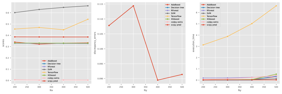
Figure 2.10: RMSE, MMD and execution time

In Figure 2.9, we can observe the extrapolation performance of each method. It is evident that the periodic kernel-based method outperforms the other methods in the extrapolation range between $[-1.5,-1]$ and $[1,1.5]$. This finding is also supported by Figure 2.10, which shows the RMSE error for different sample sizes $N_{x}$.

It is important to note that the choice of method does not affect the function norms and the discrepancy errors. Although the periodic kernel-based method performs better in this example, our goal is not to establish its superiority. Instead, we aim to present a benchmark methodology, especially when extrapolating test set data that are far from the training set.

2.4.3 Extrapolation in two dimensions

Description. In this section, we demonstrate that the dimensionality of the problem does not affect the performance of benchmark methods. To illustrate this point, we repeat the same steps as in the previous section, but with $D=2$ (i.e., a two-dimensional case). The reader can test with different values of $D$.

We generate data using five scenarios from Table 2.3 and visualize the results using Figure 2.11. The left and right plots show the training set $(X,f(X))$ and the test set $(Z,f(Z))$, respectively. Note that $f$ is the two-dimensional periodic function defined at (2.4.1).

If the dimensionality is greater than two, we use a two-dimensional visualization by plotting $\tilde{X},f(X)$, where $\tilde{X}$ is obtained either by setting indices $\tilde{X}=X[index1,index2]$ or by performing a principal component analysis (PCA) over $X$ and setting $\tilde{X}=\text{PCA}(X)[index1,index2]$.

Figure 2.11: Train set vs test set.

A comparison between methods. We compare the performance of two models for function extrapolation: CodPy periodic Gaussian kernel and SciPy RBF kernel. We assess their accuracy on the first two scenarios defined in Table 2.3 and present the results in the first two graphs of Figure 2.12, which show the RBF kernel predictions. The last two graphs in the figure show the periodic Gaussian kernel predictions.

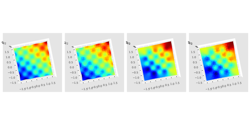
Figure 2.12: RBF (first and second) and periodic Gaussian kernel (third and forth)

2.4.4 Clustering

Description. We briefly overview here our methodology (which will be fully described in the next chapter). Specifically, we proceed as follows.

• Demonstrate the prediction function $\mathcal{P}_{m}$ for some methods in the context of supervised learning. Compute some performance indicators and present a toy benchmark using these indicators.

• To generate data, we use a multimodal and multivariate Gaussian distribution with a covariance matrix $\Sigma=\sigma I_{d}$. The goal is to identify the modes of the distribution using a clustering method.

We will generate distributions with a predetermined number of modes, which will enable us to test validation scores on this toy example.

A comparison between methods. In this section, we evaluate and compare the performance of CodPy clustering MMD minimization with Scikit implementation of the k-means algorithm in order to identify the modes of a multimodal and multivariate Gaussian distribution. We generate distributions with different numbers of modes (ranging from 2 to 6) and test validation scores on this toy example.

Figure 2.14 displays the computed clusters using a k-means algorithm (top row) and the MMD minimization (bottom row) for two different scenarios. The four confusion matrices in the figure correspond to the two clustering methods for each scenario.

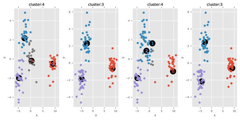
Figure 2.13: Scatter plots of k-means and MMD minimization algorithms

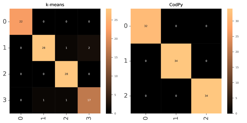
Figure 2.14: Confusion matrices of k-means and MMD minimization algorithms

We evaluate the performance of various methods using performance indicators, as shown in Figure 2.15. To assess the performance of the algorithms, we use inertia as the metric since it is a common measure of clustering quality. The MMD error indicates the degree to which two samples are the same, and it is computed at different sample sizes. The results of this test are summarized in Table LABEL:tab:2999 in the appendix to this chapter.

Overall, our aim is to offer a thorough comparison of the two clustering methods. This will enable readers to make informed decisions about which method is best suited for different scenarios.

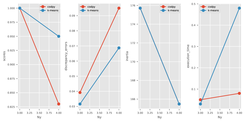
Figure 2.15: benchmark of various performance indicators for clustering.

2.5 Bibliography

XGBoost is a computationally efficient implementation of the original gradient boost algorithm and is commonly used for large-scale data sets with complex features. TensorFlow is a popular library for building and training neural networks, often used for image and speech recognition. PyTorch is another popular library for building and training neural networks, known for its dynamic computational graph and ease of use. Scikit-learn offers a comprehensive set of models for linear, SVM, and feature selection methods, making it a popular choice for general machine learning tasks. TensorFlow Probability is a recent addition to the TensorFlow library and focuses on probabilistic modeling and Bayesian inference.

2.6 Appendix to Chapter 2

Results concerning 1D extrapolation. In Table LABEL:tab:2998 we present the performance of several supervised machine learning models in extrapolating the values of a periodic function defined at (2.4.1). The comparison is based on four measures: execution time, scores, the norm of the predicted function, and MMD errors.

Table 2.4: Supervised algorithm performance indicators

$predictors$	$D$	$N_{x}$	$N_{y}$	$N_{z}$	$D_{f}$	time	RMSE	MMD
codpy extra	1	500	500	500	1	0.41	0.0035	0.0914
codpy extra	1	400	400	400	1	0.23	0.0046	0.0895
codpy extra	1	300	300	300	1	0.12	0.0033	0.1144
codpy extra	1	200	200	200	1	0.05	0.0064	0.1078
scipy pred	1	500	500	500	1	0.02	0.3855	0.0914
scipy pred	1	400	400	400	1	0.02	0.3856	0.0895
scipy pred	1	300	300	300	1	0.02	0.3859	0.1144
scipy pred	1	200	200	200	1	0.02	0.3865	0.1078
SVM	1	500	500	500	1	0.12	0.6616	0.0914
SVM	1	400	400	400	1	0.03	0.6478	0.0895
SVM	1	300	300	300	1	0.02	0.6293	0.1144
SVM	1	200	200	200	1	0.00	0.6015	0.1078
Tensorflow	1	500	500	500	1	6.60	0.5424	0.0914
Tensorflow	1	400	400	400	1	5.02	0.4494	0.0895
Tensorflow	1	300	300	300	1	3.88	0.4699	0.1144
Tensorflow	1	200	200	200	1	3.13	0.4560	0.1078
Decision tree	1	500	500	500	1	0.35	0.3277	0.0914
Decision tree	1	400	400	400	1	0.00	0.3280	0.0895
Decision tree	1	300	300	300	1	0.00	0.3285	0.1144
Decision tree	1	200	200	200	1	0.00	0.3294	0.1078
AdaBoost	1	500	500	500	1	0.30	0.3335	0.0914
AdaBoost	1	400	400	400	1	0.05	0.3309	0.0895
AdaBoost	1	300	300	300	1	0.03	0.3216	0.1144
AdaBoost	1	200	200	200	1	0.02	0.3404	0.1078
XGboost	1	500	500	500	1	0.53	0.3304	0.0914
XGboost	1	400	400	400	1	0.05	0.3307	0.0895
XGboost	1	300	300	300	1	0.03	0.3312	0.1144
XGboost	1	200	200	200	1	0.03	0.3320	0.1078
RForest	1	500	500	500	1	0.29	0.3279	0.0914
RForest	1	400	400	400	1	0.25	0.3283	0.0895
RForest	1	300	300	300	1	0.20	0.3287	0.1144
RForest	1	200	200	200	1	0.19	0.3297	0.1078

Results concerning 2D extrapolation. We conducted several tests for various scenarios in 2D extrapolation using CodPy Gaussian kernel approach. The scenarios involve predicting the value of a function for different input points outside the training set. The computed indicators include the root mean squared error (RMSE), MMD, the norm of the predicted function and the execution time of the algorithm. The results are summarized in Table 2.5.

Table 2.5: Supervised algorithm performance indicators

$predictors$	$D$	$N_{x}$	$N_{y}$	$N_{z}$	$D_{f}$	time	RMSE	MMD
codpy extra	2	1024	900	1024	1	2.90	0.0003	0.1103
codpy extra	2	484	400	484	1	0.54	0.0002	0.1856
scipy pred	2	1024	900	1024	1	0.16	0.2077	0.1103
scipy pred	2	484	400	484	1	0.02	0.2168	0.1856

Results concerning the clustering methods. In this test, we evaluate and compare the performance of two different clustering methods, CodPy clustering MMD minimization and Scikit implementation of k-means algorithm, on identifying the modes of a multimodal and multivariate Gaussian distribution. Distributions with different numbers of modes, ranging from 2 to 6, are generated to test the validation scores on this toy example.

The results are presented in Table LABEL:tab:2999, which summarizes the performance of the two methods using four indicators: execution time, scores, MMD, and inertia. To evaluate the performance of the algorithms, we chose inertia as the metric for comparison, to avoid confusion in defining the best possible clustering. The MMD error simply indicates when two samples are the same and coincide at different levels of sample size.

Table 2.6: Unsupervised algorithms performance indicators (Clustering)

$predictors$	$D$	$N_{x}$	$N_{y}$	$N_{z}$	$D_{f}$	time	scores	MMD	inertia
k-means	2	100	4	100	1	0.48	0.95	0.0687	165.48
k-means	2	100	3	100	1	0.03	1.00	0.0316	175.71
codpy	2	100	4	100	1	0.08	0.83	0.0950	165.48
codpy	2	100	3	100	1	0.05	1.00	0.0392	175.71

Chapter 3 Basic notions about reproducing kernels

3.1 Purpose of this chapter

3.1.1 Basic terminology

We begin the presentation of our methods with the notion of reproducing kernels, which plays a pivotal role in building representations and approximations of, both, data and solutions, in combination with several other features at the core of our CodPy algorithms, notably the introduction of transformation maps. These maps offer the flexibility to tailor basic kernels to address specific challenges. Together with the notion of kernel-based operators we will define mesh-free discretization algorithms, and our methodology will provide a versatile framework for machine learning and PDEs applications. For the present chapter, we focus our attention on the notion of kernels.

We begin with some notation in agreement with the one already put forward in the previous chapter. A set of $N_{x}$ variables in $D$ dimensions, denoted by $X\in\mathbb{R}^{N_{x},D}$, is provided to us, together with a $D_{f}$-dimensional vector-valued data function $f(X)\in\mathbb{R}^{N_{x},D_{f}}$ which represents the training values associated with the training set $X$, as they are called. At this stage, the function $f$ is known only at the collection of points $X$. The input data therefore consists of

$$(X,f(X))=\{(x^{n},f(x^{n})\}_{n=1,\dots,N_{x}},\qquad X\in\mathbb{R}^{N_{x},D},\qquad f(X)\in\mathbb{R}^{N_{x},D_{f}}.$$

We are interested in predicting the so-called test values $f_{Z}\in\mathbb{R}^{N_{z},D_{f}}$ on a new set of variables called the test set $Z\in\mathbb{R}^{N_{z},D}$ and denoted by

$$(Z,f_{Z})=\{(z^{n},f_{z}^{n})\}_{n=1,\dots,N_{z}},\qquad Z\in\mathbb{R}^{N_{z},D},\qquad f_{Z}\in\mathbb{R}^{N_{z},D_{f}}.$$ (3.1.1)

Let us point out immediately that, throughout this chapter, we will illustrate our notions for the dimensions given in the tables for extrapolation and for interpolation, and with a choice of function consisting of the sum of a periodic function and a direction-wise increasing function, given by

$$f(x)=f(x_{1},\ldots,x_{D})=\prod_{d=1,\ldots,D}\cos(4\pi x_{d})+\sum_{d=1,\ldots,D}x_{d},\qquad x\in\mathbb{R}^{D}.$$ (3.1.2)

Table 3.1: A choice of dimensions for data extrapolation

$D$	$N_{x}$	$N_{y}$	$N_{z}$
2	576	576	576

This numerical example will be useful in order to point out certain features enjoyed by the prediction $(Z,f_{Z})$, and compare it with the training set $(X,f(X))$.

Furthermore, we propose to introduce an additional variable denoted by $Y$, and we distinguish between several cases of interest. Throughout we use the notation $Y\in\mathbb{R}^{N_{y},D}$ and $f_{Y}\in\mathbb{R}^{N_{y},D_{f}}$, which is consistent with our notation $X\in\mathbb{R}^{N_{x},D}$, $Z\in\mathbb{R}^{N_{z},D}$ while $f(X)\in\mathbb{R}^{N_{x},D_{f}}$ and $f_{Z}\in\mathbb{R}^{N_{z},D_{f}}$.

• The choice $N_{x}=N_{z}$ corresponds to data extrapolation (as will be explained later).

• The choice $N_{y}<<N_{x}$ corresponds to data interpolation (as will also be explained later).

Table 3.2: A choice of dimensions for data projection

$D$	$N_{x}$	$N_{y}$	$N_{z}$
2	576	32	576

Hence, Figure 3.1 shows results obtained for a typical problem of machine learning. In the following discussion, we often focus on the choice made in the first test. The left-hand plots show the (variable, value) training set $(X,f_{X})$, while the right-hand plot shows the (variable, value) test set $(Z,f_{Z})$. The middle plots show the (variable, value) parameter set $(Y,f_{Y})$. The crucial role played by the additional variable $Y$ will be discussed later on: basically, it helps not only for the overall accuracy of the algorithm, but also for its overall computational cost.

Keeping in mind the above illustratve example, we now proceed with the definition and basic properties of kernels and maps of interest.

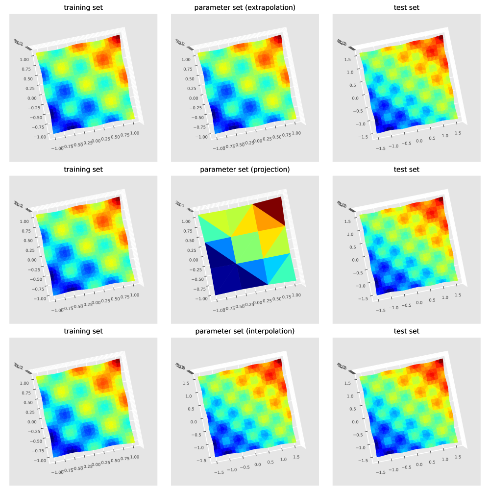
Figure 3.1: Examples of (training, parameter, test) sets for three different $Y$

3.1.2 A concrete example: images classification

It will be useful to keep in mind the following concrete case. Suppose that we are developing a images classification system. Each image is represented as a high-dimensional vector (or point in a high-dimensional space), where each component corresponds to a pixel intensity or a color value.

1. Training set: We start with a collection of $N_{x}$ images, which we will use to train our system. If we have $N_{x}$ such images and each image is represented in $D$ dimensions (e.g., $D$ is the number of pixels of each image), then our training set $X\in\mathbb{R}^{N_{x},D}$ consists of these images.

2. Training values: Along with each image in our training set, we associate a label or identifier and each label is represented as a $D_{f}$-dimensional vector. For instance, we associate for each images $x^{n}$, the label $f(x^{n})=(0,1)$ (cat), or $f(x^{n})=(1,0)$ (dog). Would there be one more labels, as "turtle", then $f(x^{n})$ would take three vector values. This way of encoding labels is called "hot encoding".

   So, for each image $x^{n}$ in our training set, we have an associated label $f(x^{n})$. Together, our input data therefore is

   $$(X,f(X))=\{(x^{n},f(x^{n})\}_{n=1,\dots,N_{x}}\in\mathbb{R}^{D_{x},D_{f}}$$

3. Test Set: Now, after training our model, we want to test its accuracy. To that aim, consider a new set of images that the system has never considered before. This is our test set $Z$. If we have $N_{z}$ such test images, each represented in $D$ dimensions, then $Z\in\mathbb{R}^{N_{z},D}$.

4. Test Values: Our goal is to predict the labels (or identifiers) for each image in our test set. These predicted labels are our test values $f_{Z}$. For each test image $z^{n}$, we want to predict a label $f_{z}^{n}$. The collection of test images and their predicted labels is:

   $$(Z,f_{Z})=\{(z^{n},f_{z}^{n})\}_{n=1,\dots,N_{z}}$$

In this facial recognition context, the training set is a collection of known faces with their associated names (or identification numbers, etc.). The test set is a collection of new faces, and our goal is to predict their names based on what our system learned from the training set.

3.2 Reproducing kernels and transformation maps

3.2.1 Kernels of interest

Positive kernels and kernel matrices. A kernel, denoted by $k:\mathbb{R}^{D}\times\mathbb{R}^{D}\to\mathbb{R}$, is a symmetric real-valued function, that is, satisfying $k(x,y)=k(y,x)$. Given two collections of points in $\mathbb{R}^{D}$, namely $X=(x^{1},\cdots,x^{N_{x}})$ and $Y=(y^{1},\cdots,y^{N_{y}})$, we define the associated kernel matrix $K(X,Y)=\big{(}k(x^{n},y^{m})\big{)}\in\mathbb{R}^{N_{x},N_{y}}$ by

$$K(X,Y)=\left(\begin{array}[]{ccc}k(x^{1},y^{1})&\cdots&k(x^{1},y^{N_{y}})\\ \ddots&\ddots&\ddots\\ k(x^{N_{x}},y^{1})&\cdots&k(x^{N_{x}},y^{N_{y}})\end{array}\right).$$ (3.2.1)

We say that $k$ is a positive kernel if, for any collection of distinct points $X\in\mathbb{R}^{N_{x},D}$ and for any collection $c^{1},...,c^{N_{x}}\in\mathbb{R}^{N_{x}}$ that is not identically vanishing, we have

$$\sum_{1\leq i,j\leq N_{x}}c^{i}c^{j}k(x^{i},x^{j})>0.$$ (3.2.2)

When $N_{x}=N_{y}$, the squared matrix $K(X,Y)$ is called the Gram matrix.

More generally, a kernel $k$ is said to be conditionally positive definite if it is positive only on a certain sub-manifold of $\mathbb{R}^{D}\times\mathbb{R}^{D}$. In other words, the positivity condition holds only when $X,Y$ are restricted to belong to this sub-manifold, which may be referred to as the “positivity domain” and, by definition, is a subset of $\mathbb{R}^{D}\times\mathbb{R}^{D}$ on which $k$ is positive definite. Outside this domain, the kernel may take vanishing or even negative values. Yet, conditionally positive definite kernels are commonly used in certain applications, for instance when the data or the problem enjoy specific geometric or topological structures. Indeed, the kernel is often designed in order to capture certain patterns of particular interest; this is relevant in, for instance, spatial statistics, computer graphics, and image processing.

Throughout this Monograph, we work with positive or conditionally positive kernels. The available kernels in the CodPy library are listed in Table LABEL:tab:302 and plotted in Figure~3.2.

Table 3.3: The list of kernels

Kernel	$k(x,y)$
1. Dot product	$k(x,y)=x^{T}y$
2. ReLU	$k(x,y)=\max(x-y,0)$
3. Gaussian	$k(x,y)=\exp(-\pi\mid x-y\mid^{2})$
4. Periodic Gaussian	$k(x,y)=\prod_{d}\theta_{3}(x_{d}-y_{d})$
5. Matern	$k(x,y)=\exp(-\mid x-y\mid)$
6. Matern tensorial	$k(x,y)=\exp(-\prod_{d}\mid x_{d}-y_{d}\mid)$
7. Matern periodic	$k(x,y)=\prod_{d}\frac{\exp(\mid x_{d}-y_{d}\mid)+\exp(1-\mid x_{d}-y_{d}\mid)}{1+\exp(1)}$
8. Multiquadric	$k(x,y)=\sqrt{1+\frac{\mid x-y\mid^{2}}{c^{2}}}$
9. Multiquadric tensorial	$k(x,y)=\prod_{d}\sqrt{1+\frac{(x_{d}-y_{d})^{2}}{c^{2}}}$
10. Sinc square tensorial	$k(x,y)=\prod_{d}\Big{(}\frac{\sin(\pi(x_{d}-y_{d}))}{\pi(x_{d}-y_{d})}\Big{)}^{2}$
11. Sinc tensorial	$k(x,y)=\prod_{d}\frac{\sin(\pi(x_{d}-y_{d}))}{\pi(x_{d}-y_{d})}$
12. Tensor	$k(x,y)=\prod_{d}\max(1-\mid x_{d}-y_{d}\mid,0)$
13. Truncated	$k(x,y)=\max(1-\mid x-y\mid,0)$
14. Truncated periodic

Here is a brief list of applications in which certain kernels are especially useful.

• The ReLU kernel or rectified linear unit kernel yields the maximum value between the difference of two given inputs and 0. This kernel is commonly used as an activation function in neural networks, which are widely used for image recognition, natural language processing, and related applications.

• The Gaussian kernel assigns higher weights to points that are closer to the center, making it useful for tasks such as image recognition, where we want to assign higher weights to pixels that are closer together. It is also commonly used in algorithms of clustering or dimensionality reduction.

• The multiquadric kernel and their associated tensor versions are based on radial basis functions and are very useful for smoothing and interpolation of scattered data. They are commonly used in weather forecasting, seismic analysis, and computer graphics.

• The Sinc kernel and Sinc square kernel in tensorial form are used in signal processing and image analysis. They model quite accurately some features, such as the periodicity in signals or images. They are commonly used in applications such as speech recognition, image denoising, and pattern recognition.

Furthermore, we emphasize that a scaling of such basic kernels is usually required in order to properly handle the input data. This is precisely the purpose of the transformation maps, discussed later on.

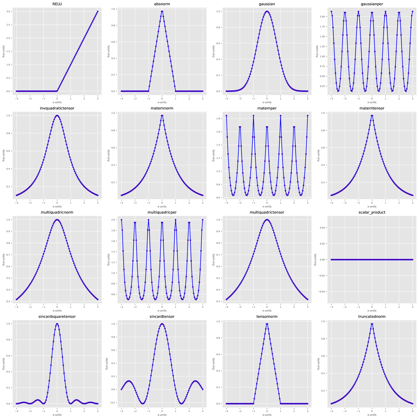
Figure 3.2: Available kernerls in the CodPy library

Examples. A mapping $S:\mathbb{R}^{D}\to\mathbb{R}^{P}$ and a function $g:\mathbb{R}\to\mathbb{R}$ being given, we construct a new kernel by setting

$$k(x,y)=g(<S(x),S(y)>_{\mathbb{R}^{P}}),\qquad x,y\in\mathbb{R}^{D},$$

in which $g$ is called the activation function and $\langle\ldots,\ldots\rangle$ denotes the standard scalar product. In particular, this includes the scalar product between successive powers of the coordinate functions $x_{d}$ and $y_{d}$, that is,

$$k(x,y)=<(1,x,x^{T}x,\ldots),(1,y,y^{T}y,\ldots)>.$$

The latter is nothing but the classical kernel associated with a linear regression based on a polynomial basis. This kernel is positive, but the null space of the associated matrix kernel is non-trivial.

We also point out that the very classical ReLU kernel given by

$$k(x,y)=\max(<x,y>+c,0)$$

($c$ being a constant) is actually a non-symmetric, hence does not directly fit in our framework but is included in our library since it provides a useful and very standard choice. \end{example}

Consider next the so-called tensornorm kernel (described below) with the relevant parameters specified in Section 3.2.1. Then we can compute its associated kernel matrix by using our function denoted by op.Knm in CodPy. Typical values for this matrix are presented in Table 3.4, which includes the first four rows and columns.

Table 3.4: First four rows and columns of the kernel matrix $K(X,Y)$

4.000000	3.873043	3.746087	3.619130
3.873043	3.833648	3.714253	3.594858
3.746087	3.714253	3.682420	3.570586
3.619130	3.594858	3.570586	3.546314

Inverse of a kernel matrix. The inverse of a kernel matrix $K(X,Y)^{-1}$ is computed in two ways depending on whether $X=Y$ or $X\neq Y$. When $X=Y$, the inverse is computed with the formula

$$K(X,X)^{-1}=(K(X,X)+\epsilon\,R)^{-1},$$

in which $\epsilon\geq 0$ is an (optional) regularization term, referred to as the Tikhonov regularization parameter, and might be required for improving the numerical stability. Here, $R$ is some given matrix, which by default is taken to be the identity matrix $I_{d}$ of dimension $N_{X},N_{X}$. By default in CodPy, $\epsilon$ takes the value $\epsilon=10^{-8}$ but can be adjusted if necessary.

When $X\neq Y$, the inverse is computed by the least-squares method, given by

$$K(X,Y)^{-1}=(K(Y,X)K(X,Y)+\epsilon R)^{-1}K(Y,X),$$ (3.2.3)

in which $R$ ow has the dimension $N_{Y},N_{Y}$. For several possible choices $R\neq I_{d}$, we refer to Figure~6.3.

Table 3.5 shows the first four rows and columns of the inverse matrix for an example matrix $K(X,Y)^{-1}\in\mathbb{R}^{N_{y},N_{x}}$ when $N_{x}=N_{y}$.

Table 3.5: First four rows and columns of an inverted kernel matrix $K(X,Y)^{-1}$

4.90e-05	4.70e-05	4.53e-05	4.28e-05
4.69e-05	4.54e-05	4.33e-05	4.14e-05
4.51e-05	4.33e-05	4.16e-05	4.02e-05
4.31e-05	4.16e-05	4.00e-05	3.87e-05

Observe that, in the following instances, the product matrix $K(X,Y)K(X,Y)^{-1}$ in Table 3.5 may not coincide with the identity matrix.

• If $N_{x}\neq N_{y}$.

• If $\epsilon>0$, the Tikhonov regularization parameter is used to adjust the solution for better stability. While the user can choose $\epsilon=0$, in certain cases this will lead to performance issues. For example, if the kernel is not unconditionally positive definite, the CodPy library may raise an exception, and switch from the standard matrix inversion method to an adapted method for non-invertible matrices, which can be computationally costly.

• If the choice of the kernel happens to lead to a matrix $K(X,X)K(X,X)^{-1}$ that does not have full rank, for instance when we use a linear regression kernel (cf. Section 3.4), the matrix becomes a projection on the null space of $K(X,X)$.

Distance matrices. Distance matrices provide a very useful tool in order to evaluate the accuracy of a computation. To any positive kernel $k:\mathbb{R}^{D},\mathbb{R}^{D}\mapsto\mathbb{R}$, we associate the distance function $d_{k}(x,y)$ defined (for $x,y\in\mathbb{R}^{D}$) by

$$d_{k}(x,y)=k(x,x)+k(y,y)-2k(x,y).$$ (3.2.4)

For positive kernels, $d_{k}(\cdot,\cdot)$ is continuous, non-negative, and satisfies the condition $d_{k}(x,x)=0$ (for all relevant $x$).

For a collection of points $X=(x^{1},...,x^{N_{x}})$ and $Y=(y^{1},...,y^{N_{y}})$ in $\mathbb{R}^{D}$, we define the associated distance matrix $D(X,Y)\in\mathbb{R}^{N_{x},N_{y}}$ by

$$D(X,Y)=\left(\begin{array}[]{ccc}d_{k}(x^{1},y^{1})&\cdots&d_{k}(x^{1},y^{M})\\ \ddots&\ddots&\ddots\\ d_{k}(x^{N},y^{1})&\cdots&d_{k}(x^{N},y^{M})\end{array}\right).$$ (3.2.5)

Distance matrices are crucial in a myriad of applications, particularly in addressing clustering and classification challenges.

Table 3.6 shows the first four columns of the kernel-based distance matrix $D(X,Y)$. As expected, the diagonal values are all vanishing.

Table 3.6: First four rows and columns of a kernel-based distance matrix $D(X,Y)$

0.00	0.08	0.16	0.24
0.08	0.00	0.08	0.16
0.16	0.08	0.00	0.08
0.24	0.16	0.08	0.00

3.2.2 Maps

A map is a function that transforms data from one space to another. When dealing with kernels, we use maps in order to transform our input data in a way that makes it easier for our kernel function to capture the underlying patterns or structures. Mappings, often denoted by $S$, take input from $\mathbb{R}^{T}$ and generate an output in $\mathbb{R}^{D}$, where $T$ and $D$, by definition, are the dimensions of the input and output spaces, respectively. We distinguish between the following maps.

• rescaling maps correspond to the choice $T=D$ and are used in order to fit data $X,Y,Z$ to the range associated with a given kernel.

• dimension-reduction maps correspond to the choice $T\leq D$.

• dimension-increasing maps correspond to the choice $T\geq D$, and are useful when adding information to the training set is required. Such a transformation might be loosely called a kernel trick.

The list of rescaling maps available in our framework can be found in Table LABEL:tab:307.

Table 3.7: List of available maps

	Maps	Formulas
1	Scale to standard deviation	$S(X)=\frac{x}{\sigma}$, $\sigma=\sqrt{\frac{1}{N_{x}}\sum_{n<N_{x}}(x^{n}-\mu)}$, $\mu=\frac{1}{N_{x}}\sum_{n<N_{x}}x^{n}.$
2	Scale to erf	$S(X)=erf(x)$, $erf$ is the standard error function.
3	Scale to erfinv	$S(X)=erf^{-1}(x)$, $erf^{-1}$ is the inverse of $erf$.
4	Scale to mean distance	$S(X)=\frac{x}{\sqrt{\alpha}}$, $\alpha=\sum_{i,k\leq N_{x}}\frac{\mid x^{i}-x^{k}\mid^{2}}{N_{x}^{2}}.$
5	Scale to min distance	$S(X)=\frac{x}{\sqrt{\alpha}}$, $\alpha=\frac{1}{N_{x}}\sum_{i\leq N_{x}}\min_{k\neq i}\mid x^{i}-x^{k}\mid^{2}.$
6	Scale to unit cube	$S(X)=\frac{x-\min_{n}{x^{n}}+\frac{0.5}{N_{x}}}{\alpha}$,$\alpha=\max_{n}{x^{n}}-\min_{n}{x^{n}}.$

Applying a map $S$ is equivalent to replacing a kernel $k(x,y)$ by the kernel $k(S(x),S(y))$. For instance, the use of the “scale-to-min distance map” is usually a good choice for Gaussian kernels, as it scales all points to the average minimum distance. As an example, we can transform the given Gaussian kernel using such a map. Note that the Gaussian setter function, by construction, uses the default map $set\_min\_distance\_map$. We refer the reader to a later discussion of all optional parameters.

$$kernel\_setters.set\_gaussian\_kernel( polynomial\_order:int=0,$$

$$regularization:float=1e-8,$$

$$set\_map=map\_setters.set\_min\_distance\_map)$$

Finally, in Figure~3.3 we illustrate the action of maps on our kernels. Here, we should compare the two-dimensional results generated with maps to the one-dimensional results generated without maps, and given earlier in Figure 3.2.

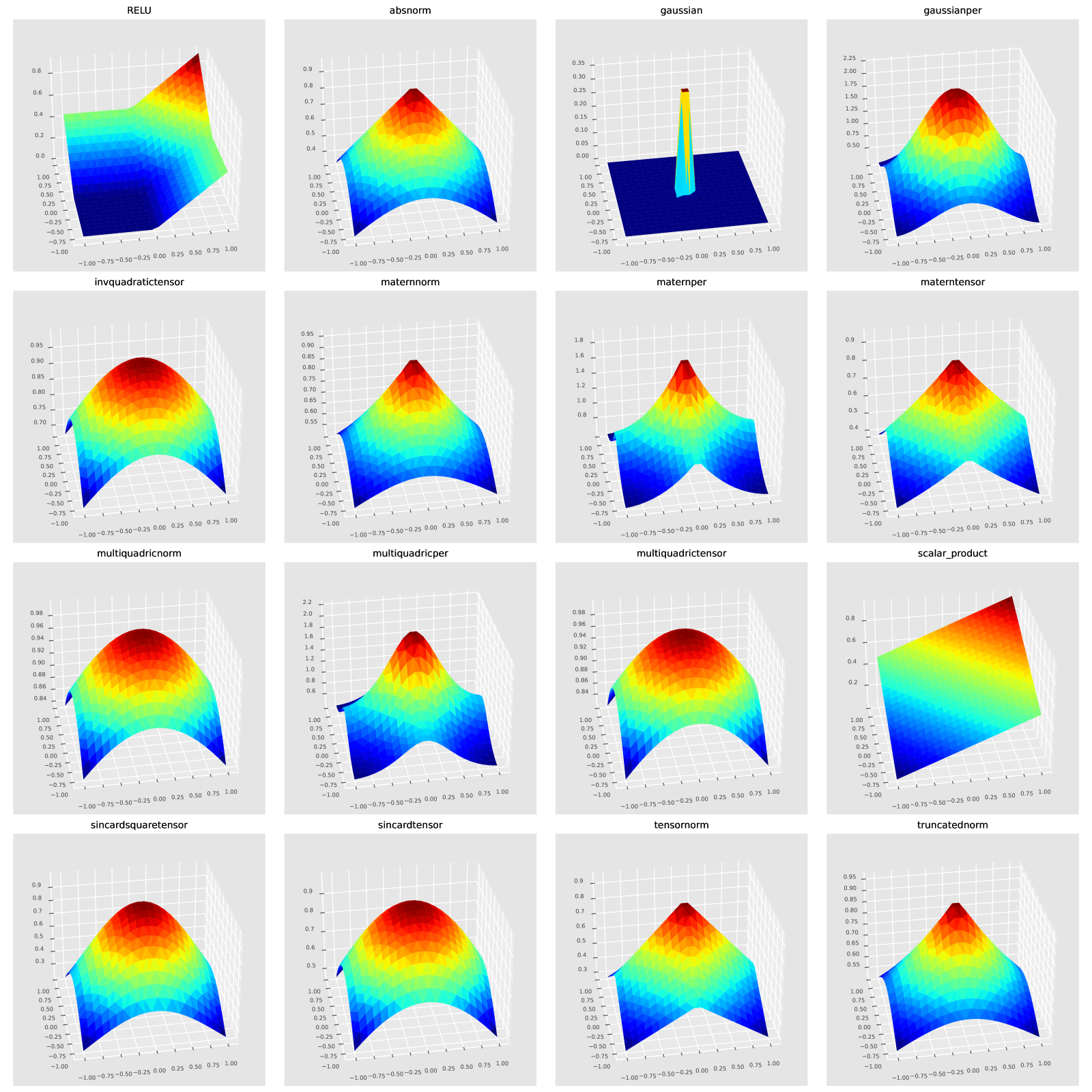
Figure 3.3: Kernels transformed with mappings

3.2.3 Discrete functional spaces

We can define a discrete vector space $\mathcal{H}_{k}^{X}$ by considering all linear combinations of the basis functions $x\mapsto k(x,x^{n})$ generated by a given finite collection of points $X=[x^{1},\dots,x^{N_{x}}]$. Here, $x^{i}\in\mathbb{R}^{D}$ for $i=1,\dots,N_{x}$. In other words, we define

$$\mathcal{H}_{k}^{X}=\Big{\{}\sum_{1\leq m\leq N_{x}}a_{m}k(\cdot,x^{m})\,/\,a=(a^{1},\ldots,a^{N_{x}})\in\mathbb{R}^{N_{x}}\Big{\}}.$$ (3.2.6)

More generally, a functional space denoted by $\mathcal{H}_{k}$ could also be defined, at least formally (or by applying a further completion argument which we are not going to elaborate upon here), by

$$\mathcal{H}_{k}=\text{Span}\big{\{}k(\cdot,x)\,/\,x\in\mathbb{R}^{D}\big{\}},$$ (3.2.7)

which consists of all linear combinations of the functions $k(x,\cdot)$ and is endowed with the scalar product

$$\big{\langle}k(\cdot,x),k(\cdot,y)\big{\rangle}_{\mathcal{H}_{k}}=k(x,y),\qquad x,y\in\mathbb{R}^{D}.$$ (3.2.8)

In every finite dimensional subspace $\mathcal{H}_{k}^{x}\subset\mathcal{H}_{k}$, according to the expression of the scalar product we can write

$$\big{\langle}k(\cdot,x^{i}),k(\cdot,x^{j})\big{\rangle}_{\mathcal{H}_{k}^{x}}=k(x^{i},x)K(X,X)^{-1}k(x,x^{j})=k(x^{i},x^{j}),\qquad i,j=1,...,N_{x}.$$ (3.2.9)

The norm of a function $f$ in the space $\mathcal{H}_{k}$ depends upon the choice of the kernel $k$. A reasonable approximation of this norm can be induced by the kernel matrix $K$, and is given by the expression

$$\|f\|_{\mathcal{H}_{k}}^{2}\simeq f(X)^{T}K(X,X)^{-1}f(X)$$

Of course, this norm could be computed after a rescaling of the kernel based on a map. Finally, we point out that the norm can be computed in CodPy by using the function

$$op.norm(X,Y,Z,f(X),set\_codpy\_kernel=None,rescale=True).$$

3.3 Interpolations and extrapolation operators

3.3.1 Proposed methodology

Our algorithms will provide us with general functions in order to make predictions, once a kernel is chosen. That is, the operator

$$f_{z}=\mathcal{P}_{k}(X,Y,Z)f(X)=K(Z,Y)K(X,Y)^{-1}f(X),$$ (3.3.1)

$$K(Z,Y)\in\mathbb{R}^{N_{z},N_{y}},K(X,Y)\in\mathbb{R}^{N_{x},N_{y}}$$

is a supervised learning machine, which we call a feed-forward operator. Here, $A^{-1}=(A^{T}A)^{-1}A^{T}$ denotes the least-square inverse of a matrix $A$. In particular, we refer to $z\mapsto\mathcal{P}_{k}(X,Y,z)\in\mathbb{R}^{N_{x}}$ as the projection operator, as this is the projection of a function on the discrete space $\mathcal{H}_{k}^{X}$;it is well-defined once a kernel $k$ has been chosen. Observe that (3.3.1) includes two contributions, namely the kernel matrix $K(X,Y)$ and the projection set of variables denoted by $Y\in\mathbb{R}^{N_{y},D}$.

To motivate the role of the argument $Y$, let us consider two particular choices that do not depend upon $Y$.

$$\text{Extrapolation operator: }\mathcal{P}_{k}(X,Z)=K(Z,X)K(X,X)^{-1}.$$ (3.3.2)

$$\text{Interpolation operator: }\mathcal{P}_{k}(X,Z)=K(X,Z)^{-1}K(X,X).$$ (3.3.3)

In some applications, these operators may lead to certain computational issues, due to the fact that the kernel matrix $K(X,X)\in\mathbb{R}^{N_{x},N_{x}}$ must be inverted as is clear from (3.3.1): this is a rather costly computational process in presence of a large set of input data. Precisely, this is our motivation for introducing the additional variable $Y$ which has the effect of lowering the computational cost. It reduces the overall algorithmic complexity of (3.3.1) to the order

$$D\,\big{(}(N_{y})^{3}+(N_{y})^{2}N_{x}+(N_{y})^{2}N_{z}\big{)}.$$

Importantly, the projection operator $\mathcal{P}_{k}$ is linear in term of, both, input and output data. Hence, while keeping the set $Y$ to a reasonable size, we can consider large set of data, as input or output.

Furthermore, choosing a well-adapted set $Y$ often is a major source of optimization. We are going to use this idea intensively in several applications. For instance, the kernel clustering method (which we will describe later on) aims at minimizing the error implied by our learning machine with respect to the set $Y=\mathcal{P}_{k}(X,Z)$. This technique also connects with the idea of sharp discrepancy sequences to be defined later on. We refer to this step as a learning process, since this is exactly the counterpart of the weight set for the neural network approach. This construction amounts to define a feed-backward machine, analogous to (3.3.1) by

$$f_{z}=\mathcal{P}_{k}(X,\mathcal{P}_{k}(X,Z),Z)f(X).$$

Observe that (3.3.1) allows us also to compute the operator

$$(\nabla f)(Z)=(\nabla\mathcal{P}_{k})(X,Y,Z)f(X)=(\nabla_{z}k)(Z,Y)K(X,Y)^{-1}f(X)\in\mathbb{R}^{D\times N_{z},D_{f}},$$ (3.3.4)

where $\nabla=(\partial_{1},\ldots,\partial_{D})$ stands for the gradient, that is, $\nabla\mathcal{P}_{k}\in\mathbb{R}^{D,N_{z},N_{x}}$ is interpreted as a tensor operator. This operator is described later on (in Section 4.2) together with many other discrete differential operators. In turn, such operators will be used in the design of computational methods for a variety of PDEs problems, and these methods are thus naturally referred to as the differential learning machine methods.

3.3.2 Extrapolation, interpolation, and projection

In our framework, the Python function associated with the projection operator $\mathcal{P}_{k}$ is based on the definition (3.3.1) and reads

$$f_{z}=\text{op.projection}(X,Y,Z,f(X)=[],k=None,rescale=False)\in\mathbb{R}^{N_{z},D_{f}}.$$ (3.3.5)

This function includes the following optional arguments.

• The function $f(X)$ is optional and allows the user to recover the whole matrix $\mathcal{P}_{k}(X,Y,Z)\in\mathbb{R}^{N_{z},N_{x}}$, if necessary.

• The kernel $k$ is optional and this provides the user with the freedom to keep the input kernel that may have been already chosen.

• The optional value rescale is chosen to be “false’ ’ by default, and this allows for calling the map prior to performing the projection operation (3.3.1). This may be helpful in order to compute the internal states of the map before performing a suitable data scaling. For instance, a rescaling will compute the parameter $\alpha$ associated with the set ($X,Y,Z$).

Interpolation and extrapolation functions in the CodPy framework are, in agreement with (3.3.2), explicit transformations applied to the operator $\mathcal{P}_{k}$, as is clear from (3.3.5). One main issue arising at this stage is to decide whether the approximation $f_{z}$ compares well to the genuine values $f(Z)$. This important issue will addressed later on:

$$f_{z} =\text{op.extrapolation}(X,Z,f(X)=[],\ldots),$$ (3.3.6)

$$f_{z} =\text{op.interpolation}(X,Z,f(X)=[],\ldots).$$

3.3.3 Error estimates based on the kernel-based discrepancy

In view of the notation for the projection operator (3.3.1), the following error estimate holds:

$$\Bigg{|}\frac{1}{N_{x}}\sum_{n=1}^{N_{x}}f(x^{n})-\frac{1}{N_{z}}\sum_{n=1}^{N_{z}}f_{z^{n}}\Bigg{|}\leq\Big{(}d_{k}\big{(}X,Y\big{)}+d_{k}\big{(}Y,Z\big{)}\Big{)}\,\|f\|_{\mathcal{H}_{k}}$$

for any vector-valued function $f:\mathbb{R}^{D}\to\mathbb{R}^{D_{f}}$. Observe that this formula is computationally realistic and can be systematically applied in order check the validity of a given kernel machine. Moreover, it can also be combined with any other type of error measure. We also emphasize the following error formula:

$$\big{\|}f(Z)-f_{z}\big{\|}_{\ell^{2}(N_{z})^{D_{f}}}\leq\Big{(}d_{k}\big{(}X,Y\big{)}+d_{k}\big{(}Y,Z\big{)}\Big{)}\|f\|_{\mathcal{H}_{k}}.$$ (3.3.7)

The key term $\big{(}d_{k}\big{(}X,Y\big{)}+d_{k}\big{(}Y,Z\big{)}\big{)}$ above is a kernel-related distance between a set of points which we refer to as the discrepancy functional. This distance is also known in the literature as the maximum mean discrepancy (MMD) (first introduced in [14]). It is a rather natural quantity, and we expect that the accuracy of an extrapolation diminishes when the extrapolation set $Z$ becomes very different from the sampling set $X$. This distance is defined by

$$d_{k}\big{(}X,Y\big{)}^{2}=\frac{1}{N_{x}^{2}}\sum_{n=1,m=1}^{N_{x},N_{x}}k\big{(}x^{n},x^{m}\big{)}+\frac{1}{N_{y}^{2}}\sum_{n=1,m=1}^{N_{y},N_{y}}k\big{(}y^{n},y^{m}\big{)}-\frac{2}{N_{x}N_{y}}\sum_{n=1,m=1}^{N_{x},N_{y}}k\big{(}x^{n},y^{m}\big{)}$$ (3.3.8)

and can be computed in CodPy with

$$op.discrepancy(X,Y,Z,set\_codpy\_kernel=None,rescale=True)$$

It is important to keep in mind the rescaling effect caused by the variable rescale. We will analyze some properties of this functional in later on (cf.~Section 4.3.5). In our presentation, we use the terms “generalized MMD” and “discrepancy error” interchangeably.

3.4 Kernel engineering

3.4.1 Transformations of kernels

We now present some operations that can be performed on kernels, and allow us to produce new, and relevant, kernels. These operations preserve the positivity property which we require for kernels. In this discussion, we are given two kernels denoted by $k_{i}(x,y):\mathbb{R}^{D},\mathbb{R}^{D}\mapsto\mathbb{R}$ (with $i=1,2$) and their corresponding matrices are denoted by $K_{1}$ and $K_{2}$. According to (3.3.1), we introduce the two projection operators

$$\mathcal{P}_{k_{i}}(X,Y,Z)=K_{i}(Z,Y)K_{i}(X,Y)^{-1}\in\mathbb{R}^{N_{z},N_{x}},\qquad i=1,2$$ (3.4.1)

In order to work with multiple kernels, in CodPy we provide two Python functions, referred to as basic setters and getters:

get_kernel_ptr(),     *set_kernel_ptr(kernel_ptr)*.

The former allows us to recover a kernel that was previously input in our library, while the latter enables us to incorporate the choice of a new kernel into our framework.

3.4.2 Adding kernels

The operation $k_{1}+k_{2}$ is defined from any two kernels and consists of adding the two kernels straightfordwardly. If $K_{1}$ and $K_{2}$ are the kernel matrices associated with the kernels $k_{1}$ and $k_{2}$, then we define the sum as $K(X,Y)\in\mathbb{R}^{N_{x},N_{y}}$ with corresponding projection $\mathcal{P}_{k}(X,Y,Z)\in\mathbb{R}^{N_{z},N_{y}}$, as follows:

$$K(X,Y)=K_{1}(X,Y)+K_{2}(X,Y),\quad\mathcal{P}_{k}(X,Y,Z)=K(Z,X)K(X,Y)^{-1}.$$ (3.4.2)

The functional space generated by $k_{1}+k_{2}$ is then

$$\mathcal{H}_{k}=\Big{\{}\sum_{1\leq m\leq N_{x}}a^{m}(k_{1}(\cdot,x^{m})+k_{2}(\cdot,x^{m}))\Big{\}}.$$ (3.4.3)

3.4.3 Multiplying kernels

A second operation $k_{1}\cdot k_{2}$ is also defined from any two kernels and consists in multiplying the kernels together. A kernel matrix $K(X,Y)\in\mathbb{R}^{N_{x},N_{y}}$ and a projection operator $\mathcal{P}_{k}(X,Y,Z)\in\mathbb{R}^{N_{z},N_{y}}$ corresponding to the product of two kernels are defined as

$$K(X,Y)=K_{1}(X,Y)\circ K_{2}(X,Y),\qquad\mathcal{P}_{k}(X,Y,Z)=K(Z,X)K(X,Y)^{-1},$$ (3.4.4)

where $\circ$ denotes the Hadamard product of two matrices. The functional space generated by $k_{1}\cdot k_{2}$ is

$$\mathcal{H}_{k}=\Big{\{}\sum_{1\leq m\leq N_{x}}a^{m}k_{1}(\cdot,x^{m})\,k_{2}(\cdot,x^{m})\Big{\}}.$$ (3.4.5)

3.4.4 Convolution kernels

Our next operation, denoted by $k_{1}\ast k_{2}$, is defined for any two kernels and consists in multiplying together the kernel matrices $K_{1}$ and $K_{2}$ as follows:

$$K(X,Y)=K_{1}(X,Y)K_{2}(Y,Y),$$ (3.4.6)

where $K_{1}(X,Y)K_{2}(Y,Y)$ stands for the standard matrix multiplication. The projection operator is given by $\mathcal{P}_{k}(X,Y,Z)=K(Z,X)K(X,Y)^{-1}$. Assuming that $k_{1}(x,y)=\varphi_{1}(x-y)$, $k_{2}(x,y)=\varphi_{2}(x-y)$, then the discrete functional space generated by $k_{1}\ast k_{2}$ is

$$\mathcal{H}_{k}=\Big{\{}\sum_{1\leq m\leq N_{x}}a^{m}k(\cdot,x^{m})\Big{\}},$$ (3.4.7)

where $k(x,y)=\Big{(}\varphi_{1}\ast\varphi_{2}\Big{)}(x-y)$ is the convolution of the two kernels.

3.4.5 Piped kernels

Let us introduce yet another approach for generating new kernels explicitly. We denote our new kernel by $k_{1}|k_{2}$ and we proceed by writing first the projection operator (3.3.5) as follows:

$$\mathcal{P}_{k}(X,Y,Z)=\mathcal{P}_{k_{1}}(X,Y,Z)\pi_{1}(X,Y)+\mathcal{P}_{k_{2}}(X,Y,Z)\Big{(}I_{d}-\pi_{1}(X,Y)\Big{)},$$ (3.4.8)

where we have set

$$\pi_{1}(X,Y)=K_{1}(X,Y)K_{1}(X,Y)^{-1}=\mathcal{P}_{k_{1}}(X,Y,X).$$

Hence, we split the projection operator $\mathcal{P}_{k}(X,Y,Z)$ into two parts. The first part is dealt with by a single kernel, while the second kernel handles the remaining error. This is equivalent to applying a Gram-Schmidt orthogonalization process of the functional spaces $\mathcal{H}_{k_{1}}^{x}$, $\mathcal{H}_{k_{2}}^{x}$, and the corresponding functional space associated with (3.4.8) reads

$$\mathcal{H}_{k}^{X}=\Big{\{}\sum_{1\leq m\leq N_{x}}a^{m}k_{1}(\cdot,x^{m})+\sum_{1\leq m\leq N_{x}}b^{m}k_{2}(\cdot,x^{m})\Big{\}}.$$ (3.4.9)

Hence, this doubles up the coefficients (4.2.1). We define its inverse matrix by concatenation:

$$K^{-1}(X,Y)=\Big{(}K_{1}(X,Y)^{-1},K_{2}(X,Y)^{-1}\big{(}I_{N_{x}}-\pi_{1}(X,Y)\big{)}\Big{)}\in\mathbb{R}^{2N_{y},N_{x}}.$$ (3.4.10)

The kernel matrix associated to a “piped kernel” pair is then

$$K(X,Y)=\Big{(}K_{1}(X,Y),K_{2}(X,Y)\Big{)}\in\mathbb{R}^{N_{x},2N_{y}}.$$ (3.4.11)

3.4.6 Piping scalar product kernels: an example with a polynomial regression

Consider a map $S:\mathbb{R}^{D}\to\mathbb{R}^{N}$ associated with a family of $N$ basis functions denoted by $\varphi_{n}$, namely $S(x)=\big{(}\varphi_{1}(x),\ldots,\varphi_{N}(x)\big{)}$. Let us introduce the dot product kernel

$$k_{1}(x,y)=<S(x),S(y)>,$$ (3.4.12)

which can be checked to be conditionally positive-definite. Let us also consider a pipe kernel denoted as $k_{1}|k_{2}$, where $k_{1}$ and $k_{2}$ are positive kernels. This construction becomes especially useful in combination with a polynomial basis function $S(x)=\big{(}1,x_{1},\ldots\big{)}$. The pipe kernel allows us for a classical polynomial regression, which enables an exact matching of the moments of a distribution. Namely, any remaining error can be effectively handled by the second kernel $k_{2}$. Importantly, this combination of kernels provides a powerful framework for modeling and capturing complex relationships between variables.

3.4.7 Neural networks viewed as kernel methods

Our setup alo encompasses strategies that were developed in the context of deep learning methods, specifically methods based on neural networks. Specifically, let us consider a feed-forward neural network consisting of $M$ layers, which can be defined by the following equations:

$$z_{m}=y_{m}g_{m-1}(z_{m-1})\in\mathbb{R}^{N_{m}},\qquad y_{m}\in\mathbb{R}^{N_{m},N_{m-1}},\qquad z_{0}=y_{0}\in\mathbb{R}^{N_{0}}.$$

Here, $y_{0},\ldots,y_{M}$ are weights and $g_{m}$ as prescribed activation functions. By concatenation, we obtain the function

$$z_{M}(y)=y_{M}z_{M-1}(y_{0},\ldots,y_{M-1}):\mathbb{R}^{N_{0},\ldots,N_{M}}\mapsto\mathbb{R}^{N_{M}}.$$

This neural network is entirely represented by the kernel composition

$$k(y_{m},\ldots,y_{0})=k_{m}\Big{(}y_{m},k_{m-1}\big{(}\ldots,k_{1}(y_{1},y_{0})\big{)}\Big{)}\in\mathbb{R}^{N_{m},\ldots,N_{0}},$$

where $k_{m}(x,y)=g_{m-1}(xy^{T})$, if fact we have $z_{M}(y)=y_{M}k(y_{M-1},\ldots,y_{0})$.

3.5 Dealing with kernels

3.5.1 Maps and kernels

Maps can ruin your prediction. Drawing upon the notation introduced in the preceding chapter, we examine the comparison between the ground truth values $(Z,f(Z))\in\mathbb{R}^{N_{z},D}\times\mathbb{R}^{N_{z},D_{f}}$ and the corresponding predicted values $(Z,f_{z})\in\mathbb{R}^{N_{z},D}\times\mathbb{R}^{N_{z},D_{f}}$. In order to further clarify the role of distinct maps in computation, we rely on a particular map referred to as the mean distance map. This map scales all points to the average distance associated with a Gaussian kernel. The resulting plot, presented in Figure 3.4, underscores the substantial influence of maps on computational results.

It is crucial to observe that the effectiveness of a specific map can differ significantly depending upon the choice of kernel. This fact variability is illustrated further in Figure 3.4.

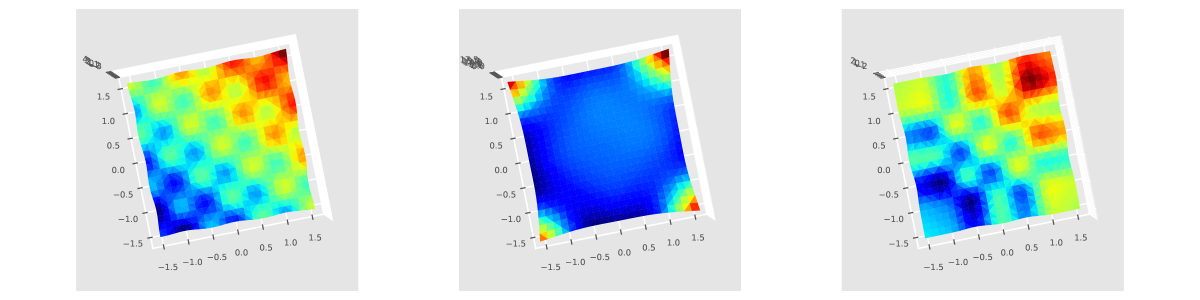
Figure 3.4: A ground truth value (first), Gaussian (second) and Matern kernels (third) with mean distance map

Composition of maps. Within our framework, we frequently employ maps to preprocess input data prior to the computation based on kernel functions or using model fitting. Each map, with its unique features, can be combined with other maps in order to craft more robust transformations. As an illustrative example, we have constructed a composite map (termed a Swiss-knife map) for Gaussian kernels, which implements multiple operations on the data.

Our composite map starts by implementing a rescaling, thereby rescaling all data points to fit within a unit hypercube. Next, the map applies the transformation $S(X)=\text{erf}^{-1}(2X-1)$, which is the inverse of the standard error function. This particular transformation is commonly employed to normalize data points to a standard normal distribution, since this has been found to enhance the performance of many machine learning algorithms.

The final step in the composite map process involves the application of the average min distance map, scaling all points by the average distance for a Gaussian kernel. This map is particularly efficient for Gaussian kernels; however, it may not be ideally suited for other types of kernels.

The implementation of this composite map in Python is performed in the following manner:

$$map\_setters.set\_min\_distance\_map(^{**}kwargs)$$

$$pipe\_map\_setters.pipe\_erfinv\_map()$$

$$pipe\_map\_setters.pipe\_unitcube\_map()$$

3.5.2 Illustration of different kernels predictions

As shown in the previous sections, the external parameters of a kernel-based prediction machine typically consist of a positive definite kernel function and a map. In addition, we need to select an inner parameter set $Y$ and distinguish between several options.

• First, we can choose $Y=X$, which corresponds to the extrapolation case and typically produces the highest accuracy; cf. Section 3.3.2.

• Alternatively, we can randomly select a subset for $Y$ from $X$, which trades accuracy for execution time and is better suited for larger training sets.

• Last, we can select $Y$ to be a sharp discrepancy sequence associated with $X$, as described in Section 4.3. This provides the best possible accuracy, but requires the use of a time-consuming numerical algorithm.

To illustrate the impact of different kernels and maps on our learning machine, we consider a one-dimensional test and compare the predictions achieved by using various kernels.

3.5.3 References

The topic of RKHS methods and kernel regressions has undergone extensive research over the past decades, resulting in a vast body of literature. In our brief list of references provided at the end of this monograph, we have included a selection of key works.

One notable resource offering a comprehensive introduction to the topic is the monograph by Hastie et al. [20], which gives fundamental material on statistical learning, including the notions of data mining, inference, and prediction. This book provides valuable insights into the field. In addition, the textbook by Berlinet and Thomas-Agnan [3] is an excellent source of material on the use of reproducing kernels in probability, statistics and related areas.

Another significant contribution to the subject can be found in the work of Smola et al. \cite{{Smola=IFI}, which also offers substantial material on the topic. We also point out here the work of Rosipal and Trejo \cite{{Rosipal} , which introduces a dimension-reduction technique for least-square models and provides a valuable perspective on the subject.

For further references, the reader should refer to the bibliography at the end of this monograph.

Chapter 4 Kernel-based operators

4.1 Introduction

We now define and study classes of operators constructed from a reproducing kernel. We start with interpolation and extrapolation operators, which are of central interest in machine learning as well as for applications to partial differential equations (PDEs). Next, we introduce distance=type measure induced by a kernel, which is referred to as the kernel discrepancy or the maximum mean discrepancy. This measure is crucial for stating error estimates and designing effective clustering methods, as we will explain in forthcoming chapters. An important tool in the present chapter is provided by kernel based discrete differential operators, such as the gradient and divergence operators. Such discrete operators will be shown to be useful in various circumstances, especially for the modeling of physical phenomena described by PDEs.

4.2 Discrete differential operators

4.2.1 Coefficient operator

We investigate first the projection operator $\mathcal{P}_{k}(X,Z,Y)$ by interpreting it in a basis function setting. With the notation in the previous chapter, given a kernel $k$ and a triple $(X,Y,Z)$ let us consider the components

$$f_{Z}=K(Z,Y)c_{Y},\quad c_{Y}=K(X,Y)^{-1}f(X)\in\mathbb{R}^{N_{Y},D_{f}},$$ (4.2.1)

where, $c_{Y}$ represents the coefficients of the decomposition of a function $f$. In other words, $f$ can be written as a linear combination of the basis functions $K(Z,y^{n})$, where $n$ ranges from $1$ to $N_{Y}$. The dimension of the coefficient matrix $c_{Y}$ is $N_{Y}\times D_{f}$ (unless composite kernels are involved).

4.2.2 Partition of unity

The notion of partition of unity is, both, a standard and a very useful concept. Let $Y\in\mathbb{R}^{N_{y},D}$ be arbitrary and let $X\mapsto\mathcal{P}_{k}(X,X,Y)$ be the projection operator associated with a kernel $k$. Using this projection we define the function

$$\phi:Y\mapsto\Big{(}\phi^{1}(Y),\ldots,\phi^{N_{x}}(Y)\Big{)}=K(Y,X)K(X,X)^{-1}\in\mathbb{R}^{N_{y},N_{x}},$$ (4.2.2)

which we refered to as the partition of unity. At every point $x^{n}$ we find

$$\phi(x^{n})=\Big{(}0,\ldots,1,\ldots,0\Big{)}=\delta_{n,m},$$ (4.2.3)

where $\delta_{n,m}$ denotes the Kronecker delta symbol (that is, $1$ if $n=m$ and $0$ otherwise). Figure 4.1 illustrates this notion with an example of four partition functions.

Figure 4.1: Four ‘partition of unity’ functions

4.2.3 Gradient operator

Next, for any positive-definite kernel $k$ we define the operator $\nabla_{k}$ over the sets of points $X,Y,Z$ by

$$\nabla_{k}(X,Y,Z)=\Big{(}\nabla_{Z}k\Big{)}(Z,Y)K(X,Y)^{-1}\in\mathbb{R}^{D,N_{x},N_{z}},$$ (4.2.4)

in which we have $\big{(}\nabla_{z}k\big{)}(Z,Y)\in\mathbb{R}^{D,N_{x},N_{y}}$. To compute the gradient of a vector-valued function $f$, we use the expression

$$(\nabla_{k}f)(Z)\sim(\nabla_{k})(Z,Y,Z)f(X)\in\mathbb{R}^{D,N_{z},D_{f}},$$

where we omit the dependency in $\nabla_{k}(X,Y,Z)$ in order to shorten the notation. Importantly, the operator $\nabla_{k}$ can be modified by maps, as we will exploit further in the next chapter. In short, we can write

$$\nabla_{k\circ S}(X,Y,Z)=(\nabla S)(Z)\Big{(}\nabla_{1}k)(S(Z),S(Y)\Big{)}K(S(X),S(Y))^{-1},$$

where $\Big{(}\nabla_{1}k\Big{)}(Z,Y)\in\mathbb{R}^{D,N_{z},N_{y}}$, and $(\nabla S)(Z)=(\partial_{d}S^{j})(Z^{n_{z}})\in\mathbb{R}^{D,D,N_{z}}$, represents the Jacobian of the map $S$, and the multiplication is defined over the first indices.

Two-dimensional example. To better understand the operator, we provide a two-dimensional example in Figure 4.2, which shows a comparison between the derivatives of the original function and their corresponding values computed using the operator (4.2.4) for the first and second dimensions. The left-hand plot corresponds to the original function, while the right-hand plot shows the computed values.

Figure 4.2: The first two graphs correspond to the first dimension (original on the left-hand, computed on the right-hand). The next two graphs correspond to the second dimension (original on the left-hand, computed on the right-hand).

4.2.4 Divergence operator

The divergence and gradient operators also play a crucial role when dealing with many differential equations. Let us indeed define the divergence operator and the transpose $\nabla_{k}^{T}$ of the operator $\nabla_{k}$.

The operator $\nabla_{k}^{T}$, by definition, is consistent with the divergence operator and reads

$$<\nabla_{k}(X,Y,Z)f(X),g(Z)>=<f(X),\nabla_{k}(X,Y,Z)^{T}g(Z)>.$$

To compute the operator $\nabla^{T}$, we start with the definition of the gradient operator (4.2.4) and define, for any $f(X)\in\mathbb{R}^{N_{x},D_{f}}$ and $g(Z)\in\mathbb{R}^{D,N_{z},D_{f}}$,

$$<\Big{(}\nabla_{z}K\Big{)}(Z,Y)K(X,Y)^{-1}f_{x},g_{z}>=<f_{x},K(X,Y)^{-T}\Big{(}\nabla_{z}K\Big{)}(Z,Y)^{T}g_{z}>.$$

The operator $\nabla_{k}(X,Y,Z)$ is then defined by

$$\nabla_{k}(X,Y,Z)^{T}=K(X,Y)^{-T}\Big{(}\nabla_{z}K\Big{)}(Z,Y)^{T}\in\mathbb{R}^{N_{x},N_{z}D},$$ (4.2.5)

where $\nabla_{z}K(Z,Y)^{T}\in\mathbb{R}^{N_{y},(N_{z}D)}$ is the transpose of the matrix $\nabla_{z}K(Z,Y)$.

A two-dimensional example. Figure 4.3 compares the outer product of the gradient to Laplace operator $\nabla_{k}(X,Y,Z)^{T}\nabla_{k}(X,Y,Z)f(X)$ to $\Delta_{k}(X,Y)f(X)$; see the next section.

Figure 4.3: Comparison of the outer product of the gradient to Laplace operator

4.2.5 Laplace operator

The Laplace operator plays also a fundamental role and relates to the ‘change in direction’ of a vector-valued function. It is defined as the divergence of the gradient of a function and is denoted by $\Delta f=\nabla^{2}f$. In a discrete setting, the Laplacian can be represented as a matrix, denoted as $\Delta_{k}(X,Y)\in\mathbb{R}^{N_{x}\times N_{x}}$, which quantifies the difference between the average value of a function and its value at each point.

This discrete Laplace operator is computed as the dot product of the transposed gradient vector and the gradient vector, as shown in (4.2.6).

$$\Delta_{k}(X,Y)=\Big{(}\nabla_{k}(X,Y,X)^{T}\Big{)}\Big{(}\nabla_{k}(X,Y,X)\Big{)}\in\mathbb{R}^{N_{x}\times N_{x}}.$$ (4.2.6)

This operator is used in various applications. In particular, the Laplacian arises for solving PDE boundary value problems (a.g. Poisson, Helmholtz), and are involved in many time evolution problems involving diffusion or propagation, as heat equations or wave equation, or stochastic martingale processes.

4.2.6 Inverse Laplace operator

The inverse Laplace operator is a useful tool in many mathematical fields, including fluid mechanics, image analysis and signal processing. It is defined as the pseudo-inverse of the Laplacian operator $\Delta_{k}(X,Y)\in\mathbb{R}^{N_{x},N_{x}}$. In other words, it provides a way to undo the effect of the Laplace operator on a function, making it useful in solving differential equations and signal filtering. The inverse Laplace operator can be computed using equation (4.2.7).

$$\Delta_{k}^{-1}(X,Y)=(\Delta_{k}(X,Y)\Big{)}^{-1}\in\mathbb{R}^{N_{x},N_{x}}.$$ (4.2.7)

A two-dimensional example. Figure 4.4 compares $f(X)$ with $\Delta_{k}(X,Y)^{-1}\Delta_{k}(X,Y)f(X)$. This latter operator is a projection operator (hence is stable).

To illustrate the use of this operator, Figure 4.4 compares the original function $f(X)$ with the result of applying the inverse Laplace operator to $\Delta_{k}(X,Y)f(X)$, i.e. $\Delta_{k}(X,Y)^{-1}\Delta_{k}(X,Y)f(X)$. This latter operator acts as a projection operator and is therefore stable.

Figure 4.4: Comparison between original function to the product of Laplace and its inverse

In Figure 4.5, we compute the operator $\Delta_{k,x,y,z}\Delta_{k,x,y,z}^{-1}f(X)$ to check that the pseudo-inverse commutes, i.e., applying the Laplacian operator and its pseudo-inverse in any order produces the same result. This property is crucial in many applications of the inverse Laplace operator.

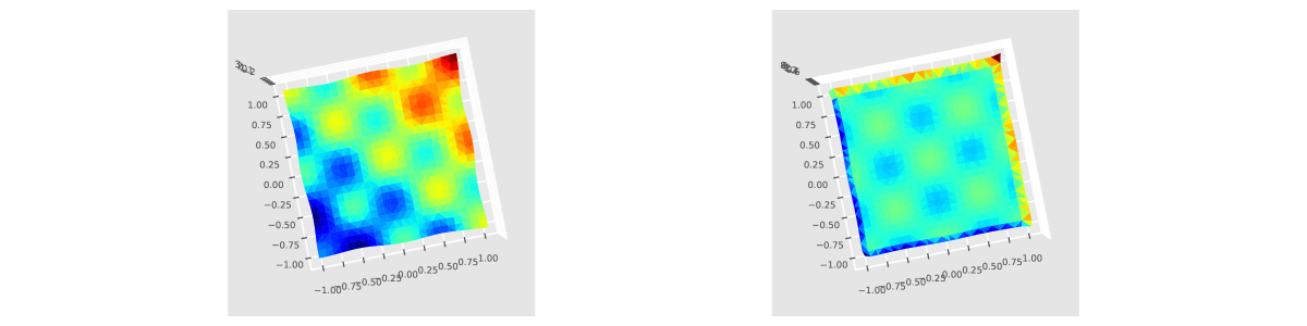
Figure 4.5: Comparison between original function and the product of the inverse of the Laplace operator and the Laplace operator

4.2.7 Integral operator - inverse gradient operator

The operator $\nabla^{-1}_{k}$ is defined as the integral-type operator

$$\nabla^{-1}_{k}=\Delta_{k}^{-1}\nabla_{k}^{T}\in\mathbb{R}^{N_{x},DN_{z}}.$$ (4.2.8)

It can be interpreted as a matrix, computed first considering $\nabla_{k}(X,Y,Z)\in\mathbb{R}^{D,N_{z},N_{x}}$, down casting it to a matrix $\mathbb{R}^{DN_{z},N_{x}}$ before performing a least-square inversion. This operator acts on any $v_{z}\in\mathbb{R}^{D,N_{z},D_{v_{z}}}$ and produces a matrix

$$\nabla^{-1}_{k}(X,Y,Z)v_{z}\in\mathbb{R}^{N_{x},D_{v_{z}}},\quad v_{z}\in\mathbb{R}^{D,N_{z},D_{v_{z}}}$$

The operator $\nabla^{-1}_{k}$ corresponds to the minimization procedure:

$$\bar{h}=\arg\inf_{h\in\mathbb{R}^{N_{x},D_{v_{z}}}}\|\nabla_{k}h-v_{z}\|_{\ell^{2}}^{2}.$$

A two-dimensional example. In Figure 4.6 we test whether

$$(\nabla_{k})^{-1}(X,Y,X)(\nabla_{k}(X,Y,X)f(X)$$

coincides or at least is a good approximation of $f(X)$. Figure 4.7 tests the extrapolation operator $(\nabla_{k})^{-1}(Z,Y,Z)(\nabla_{k}(X,Y,Z)f(X)$.

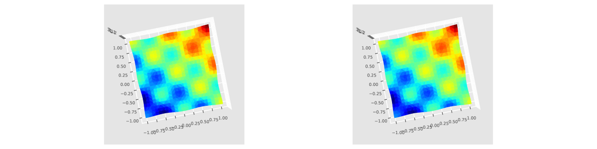
Figure 4.6: Comparison between original function to the product of the gradient operator and its inverse

Figure 4.7: Comparison between original function to the product of the inverse of the gradient operator and the gradient operator

4.2.8 Integral operator - inverse divergence operator

The following operator $(\nabla_{k}^{T})^{-1}$ is another integral-type operator of interest. We define it as the pseudo-inverse of the $\nabla^{T}$ operator by

$$(\nabla^{T}_{k}(X,Y,Z))^{-1}=\nabla_{k}(X,Y,Z)\Delta_{k}(X,Y,Z)^{-1}.$$

A two-dimensional example. We compute $\nabla_{k}(X,Y,Z)^{T}(\nabla^{T}_{k}(X,Y,Z))^{-1}=\Delta_{k}(X,Y,Z)\Delta_{k}(X,Y,Z)^{-1}$. Thus, the following computation should give comparable results as those obtained in our study of the inverse Laplace operator in Section 4.2.6.

Figure 4.8: Comparison between the product of the divergence operator and its inverse and the product of Laplace operator and its inverse

4.2.9 Leray-orthogonal operator

The Leray orthogonal operator also plays a crucial role in fluid dynamics. In particular, the Leray orthogonal operator is used for the description of incompressible fluid flows, based on the Euler or Navier-Stokes equations.

Precisely, we define the Leray-orthogonal operator as

$$L_{k}(X,Y)^{\perp}=\nabla_{k}(X,Y)\Delta_{k}(X,Y)^{-1}\nabla_{k,x,y,x}^{T}=\nabla_{k}(X,Y,Z)\nabla_{k}(X,Y,Z)^{-1}.$$

This operator acts on any vector field $f(Z)\in\mathbb{R}^{D,N_{z},D_{f}}$, and produces a three-argument object by performing a matrix multiplication after applying the input vector field:

$$L_{k}(X,Y,Z)^{\perp}f(Z)\in\mathbb{R}^{D,N_{z},D_{f}}.$$

By using the Leray-orthogonal operator, we can perform an orthogonal decomposition of any vector field into its divergence-free and curl-free components, which is the key to understanding some important structure of fluid flows.

In Figure 4.9, we compare the action of this operator on a vector field $f(Z)$ with the original function $(\nabla f)(Z)$.

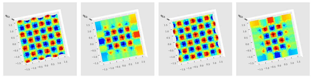
Figure 4.9: Comparing f(z) and the transpose of the Leray operator on each direction

4.2.10 Leray operator and Helmholtz-Hodge decomposition

The Helmholtz-Hodge decomposition is used in many areas of fluid mechanics, for instance in order to analyze turbulence problems, study flow past obstacles, and develop numerical methods for simulating fluid flows. One important component of this decomposition is the Leray operator, which can be used to orthogonally decompose any field. This operator is defined as follows:

$$L_{k}(X,Y,Z)=I_{d}-L_{k}(X,Y,Z)^{\perp}=I_{d}-\nabla_{k}(X,Y,Z)\Delta_{k}(X,Y,Z)^{-1}\nabla_{k}(X,Y,Z)^{T},$$

where $I_{d}$ is the identity matrix. This operator allows us to decompose any field as an orthogonal sum of two components: one part belongs to the range of the Leray operator, and one part is orthogonal to it:

$$v_{z}=L_{k}(X,Y,Z)v_{z}+L_{k}(X,Y,Z)^{\perp}v_{z},\quad<L_{k}(X,Y,Z)v_{z},L_{k}(X,Y,Z)^{\perp}v_{z}>_{D,N_{z},D_{v}}=0.$$

This decomposition is consistent with the Helmholtz-Hodge decomposition, which represents any vector field as an orthogonal sum of a gradient and a divergence-free vector:

$$v=\nabla h+\zeta,\quad\nabla\cdot\zeta=0,\quad h=\Delta^{-1}\nabla\cdot v.$$

From a numerical perspective, we can use a similar decomposition to compute the Helmholtz-Hodge decomposition. Specifically, we can decompose a vector field into a gradient component and a divergence-free component by using the Leray operator, namely

$$v_{z}=\nabla_{k}(X,Y,Z)h_{x}+\zeta_{z},\quad h_{x}=\nabla_{k}(X,Y,Z)^{-1}v_{z},\quad\zeta_{z}=L_{k}(X,Y,Z)v_{z},$$

$$\text{where}\quad\nabla_{k}(X,Y,Z)^{T}\zeta_{z}=0,\quad\left<\zeta_{z},\nabla_{k}(X,Y,Z)h_{x}\right>_{D,N_{z},D_{f}}=0.$$

This decomposition enjoys the same orthogonality properties as the ones of the original Helmholtz-Hodge decomposition. For instance, we can use this decomposition to develop numerical methods for numerically simulating fluid flows. In Figure 4.10 we compare this operator to the original function $(\nabla f)(Z)$.

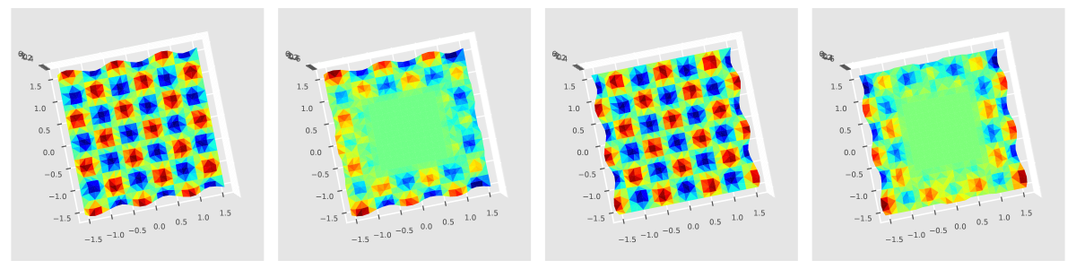
Figure 4.10: Comparing f(z) and the Leray operator in each direction

4.3 A clustering algorithm

4.3.1 Distance-based unsupervised learning machines

We now introduce a kernel-based clustering algorithm. As presented in Section 2.4.4, we illustrate the algorithm with a toy example. In Chapter 8, this algorithm is benchmarked against other popular aclustering algorithms using more concrete problems.

Our algorithm is based on distance-based minimization technique, which aims to find the minimum distance between sets of points, denoted by $d(X,Y)$, and can be expressed also as a distance between discrete measures $\mu_{x}$ and $\mu_{y}$. We are led to the following minimization problem:

$$Y=\arg\inf_{Y\in\mathbb{R}^{N_{y},D}}d(X,Y).$$ (4.3.1)

Assuming that this latter problem is well-posed and the distance functional to be convex (This is a formal argument, since most existing distances are not convex.), the cluster set $Y=\Big{(}y^{1},\ldots,y^{N_{y}}\big{)}$ can be computed. Once computed, the index function $\sigma(w,Y)=\arg\inf_{j=1\ldots N_{Y}}{d(w,y^{j})}$ can be defined, as for (2.3.4). This function can be extended naturally to define a map:

$$\sigma(Z,Y)={\sigma(z^{1},Y),\ldots,\sigma(z^{N_{z}},Y)}\in[1,\ldots,N_{y}]^{N_{z}},$$ (4.3.2)

which acts on the indices of the test set $Z$. This allows for a comparison of the prediction to a given, user-desired partition of $f(Z)$, if needed.

Note that the function $\sigma(Z,Y)$ is surjective (that is, onto), meaning that multiple points in $Z$ can be assigned to the same cluster in $Y$. Therefore, we can define its injective inverse (that is one-to-one on its image), $\sigma(Z,Y)^{-1}(n)$, which describes the points in $Z$ that are assigned to cluster $y^{n}$ in $Y$. This construction defines cells denoted as $C^{n}=\sigma(\mathbb{R}^{D},y^{n})^{-1}(n)$, which provide us with a partition of unity for the space $\mathbb{R}^{D}$.

It is worth noting that, in the context of supervised clustering methods, the training set and its values $X$ and $f(X)$, along with the index map $\sigma(X,Y)\in[1,\ldots,N_{x}]^{N_{y}}$ defined above, can be used to make predictions on the test set $Z$. Specifically, we can define a prediction for a point $z\in Z$ as

$$f_{z}=f\big{(}X^{\sigma(Y^{\sigma(z,Y)},X)}\big{)},$$ (4.3.3)

showing that a distance-minimization unsupervised algorithm can naturally be extended to a supervised one.

4.3.2 Sharp discrepancy sequences

Our kernel-based clustering algorithm can be described as follows.

• Our unsupervised clustering algorithm aims to solve the minimization problem (4.3.1) using the MMD or discrepancy functional, as described in (3.3.8). The algorithm is divided in two main steps.

  • To begin with, the goal is to find a subset of data points $Y$ that minimizes the discrepancy functional $d_{k}(X,Y)$, where $X$ is the initial set of data points and $Y$ represents the clusters. To achieve this, we solve the minimization problem (4.3.4) among all points of $X$, where $\overline{\sigma}$ is a solution of

    $$\overline{\sigma}=\arg\inf_{\sigma\in\Sigma}d_{k}(X,X^{\sigma}).$$ (4.3.4)

    Here, $\Sigma$ denotes the set of all subsets from $[1,\ldots,N_{y}]\mapsto[1,\ldots,N_{x}]$, and any solution $Y=X^{\overline{\sigma}}$ is referred to as the sharp discrepancy sequence. This minimization problem is investigated further in Chapter (4.3.5).

  • For some kernels, after the discrete minimization step described above, a simple gradient descent algorithm is used to obtain a more accurate approximation of (4.3.1). The algorithm starts with $X^{\overline{\sigma}}$ as the initial state and iteratively updates the position of each point to improve the overall solution. This approach can provide a refined and more precise solution to the original minimization problem.

• The supervised clustering algorithm involves computing the projection operator (3.3.1), that maps the test set $Z$ to the closest point in the weight set $Y$ (i.e., the sharp discrepancy sequence). This results in a prediction $f_{z}$ for each point in the test set. We implement the projection operator using the Python function (3.3.5): $f_{z}=\mathcal{P}_{k}(X,Y,Z)f(X)$.

4.3.3 Python functions

• The unsupervised clustering algorithm can be accessed through the Python function

  $$sharp\_discrepancy(X,Y=[],N_{y}=0,set\_codpy\_kernel=None,rescale=False,nmax=10).$$

• The problem (4.3.4) is at the heart of the algorithm and can be solved using the function:

  $$CodPy.alg.match(X,Y,\ldots).$$

• To compute the index associations (4.3.2), i.e., the function $\sigma_{d_{k}}(X,Y)$ use

  $$alg.distance\_labelling(X,Y,\ldots),$$

  which relies on the distance matrix $D(X,Y)$; see Section 4.

4.3.4 Impact of sharp discrepancy sequences on discrepancy errors

We now analyze of the discrepancy error for several “blob-type” toy examples, building upon the illustration in Figure 2.4.4. We set the number of “blobs” to two and generate 100 points, denoted by $N_{x}$. We follow the test methodology in Section 2.4.4 and run all tests with scenarios for $N_{y}$ covering [0,100]. Figure 4.11 compares the results for discrepancy errors of the three methods. It is visually apparent that discrepancy errors are zero, regardless of the clustering method used, when the number of clusters $N_{y}$ tends to $N_{x}$. Additionally, our kernel clustering method performs surprisingly well in terms of inertia performance indicators. This is unexpected since our method is based on discrepancy error minimization, not inertia. One possible interpretation is that the inertia functional is bounded by the discrepancy error functional.

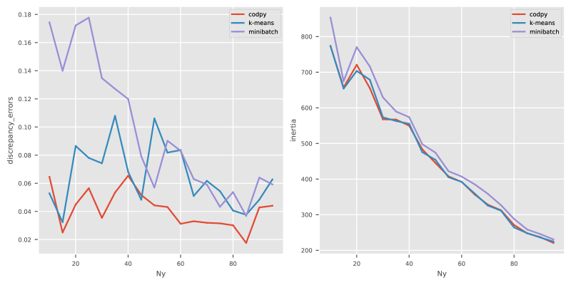
Figure 4.11: benchmark of discrepancy errors and inertia

4.3.5 A study of the discrepancy functional

As explained above, in order to compute sharp discrepancy sequences we first solve the discrete minimizing problem (4.3.1) and obtain $X^{\sigma}$ as its solution.

We then use a simple gradient descent algorithm, which depends on the kernel being used, to refine the solution. The minimizing properties of $d_{k}(X,Y)$ heavily rely on the kernel definition $k(x,y),$ and the choice of algorithm depends on the regularity of the kernel. We illustrate this numerically in this section and observe the following fact.

If the kernel is sufficiently smooth, the distance functional $d_{k}(X,Y)$ will also be smooth, and a descent algorithm based on gradient computations would be an efficient option. If the kernel is only continuous or piecewise derivable, we assume that the minimum is attained by the discrete minimum solution $X^{\sigma}$. This functional is concave almost everywhere, as shown in this section.

To illustrate this phenomenon, let us generate some random one-dimensional distributions $X\in\mathbb{R}^{N_{x}}$. We then study the following functional for three kernels:

$$y\mapsto d_{k}(X,y),$$

where $y$ is randomly generated on the unit cube. This functional represents the minimum distance to be achieved if one were to consider a single cluster.

An example of smooth kernels: Gaussian. We begin our analysis of the discrepancy functional by examining the Gaussian kernel family, which is constructed by using the following kernel, which generates functional spaces made of smooth functions:

$$k(x,y)=\exp(-(x-y)^{2})$$

In Figure 4.12, we show the function $y\mapsto d_{k}(x,y)$ in blue color. Additionally, we display the function $d_{k}(x,x^{n})$, $n=1\ldots N_{x}$ in Figure 4.12 to demonstrate that this functional is smooth but neither convex nor concave. Notably, the minimum of this functional is achieved by a point that is not part of the original distribution $X$.

For a two-dimensional example, we refer to Figure 4.13 (left-hand) for a display of this functional.

An example of Lipschitz continuous kernels: RELU. Let us now consider a kernel that generates a functional space with less regularity. The RELU kernel is the following family of kernels which essentially generates the space of functions with bounded variation:

$$k(x,y)=\max(1-|x-y|,0).$$

As shown in Figure \ref{fig:MMD1 (middle), the function $y\mapsto d_{k}(x,y)$ is only piecewise differentiable. Hence, in some cases, the functional $d_{k}(x,y)$ might have an infinite number of solutions (if a “flat” segment occurs), but a minimum is attained on the set $X$. Figure 4.13 (middle) displays the two-dimensional example.

An example of continuous kernel: Matern. The Matern family generates a space of continuous functions, and is defined by the kernel

$$k(x,y)=\exp(-|x-y|).$$

In Figure 4.12, we observe that the function $y\mapsto d_{k}(x,y)$ has concave regions almost everywhere, making it difficult to find a global minimum using a gradient descent algorithm. Figure 4.13-right displays a two-dimensional example of this functional.

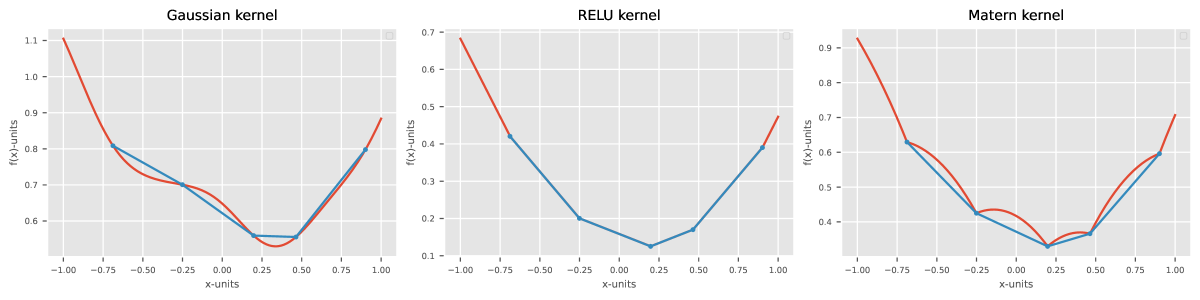
Figure 4.12: Distance functional for the Gaussian, the Matern and the RELU kernels (1D)

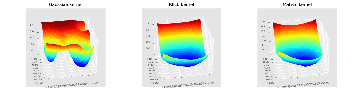
Figure 4.13: Distance functional for the Gaussian, the Matern and the RELU kernels (2D)

4.3.6 Summary of proposed methods

To conclude, we presented here several kernel-based discretizationformulas which are motivated by our aim to produce a unified framework for numerical simulation and machine learning while offering algortithms enjoying reproducibility and robustness properties.

The main tool is given by a variety of discrete differential operators, including the gradient, divergence, Laplace, and Leray-orthogonal operators. These operators are essential for applications to PDEs (which we will explore in Chapter 6).

One of the advantages of the kernel-based methodology is that it provides one with a natural way to introduce (discrepancy) error estimates, and therefore make a priori predictions about the performance of a given learning machine or simulation algorithm. This is particularly useful in unsupervised machine learning, where tone goal is to cluster data points without any knowledge of their true labels. In Chapter 5, we will show how the use of optimal transport in clustering can lead to much improved results in comparison to traditional methods.

In supervised machine learning, the goal is to predict the labels of new data points based on a training set of labeled data points. To accomplish this, we use interpolation and extrapolation methods, which are based on the idea of using a function that approximates the data points in the training set. We are going to explore these methods in Chapter 7.

Finally, in the section on generative models, we show how the use of kernel methods can be applied to generate new data points that are similar to those in the training set. This is achieved by learning a probability distribution over the data points in the training set and then sampling from this distribution to generate new data points.

Overall, the methods presented in this chapter offer a powerful and flexible framework for numerical simulations and machine learning. By leveraging the power of kernel methods and reproducing kernel Hilbert spaces, we are able to achieve both high accuracy and interpretable results. Moreover, the use of discrepancy errors allows us to make a priori predictions about the performance of a given learning machine, which can be extremely useful in practice.

4.4 Bibliography

The topic of RKHS methods and kernel regressions has been extensively studied and there is a vast literature on the subject. AS mentioned earlier, we provide a list of references at the end of this monograph. In partcular, see the references already indicated at the end of Chapter 3.

Chapter 5 Permutations and optimal transport

5.1 A brief overview of optimal transport

5.1.1 Generative methods : encoders and decoders

In the previous chapter we introduced the notion of kernel discrepancy, which allows one to measure the error associated with kernel methods and predictive machines. In this chapter, this notion of distance is used as a natural bridge with the theory of optimal transport theory [61] for a in the context of discrete problems.

Precisely, consider $\mathbb{X}\in\mathbb{R}^{D_{X}},\mathbb{Y}\in\mathbb{R}^{D_{Y}}$ any two random variables supported in $\mathcal{X},\mathcal{Y}$, denote $d\mathbb{X},d\mathbb{Y}$ their probability measure, and $X,Y\in\mathbb{R}^{N,D_{X}},\mathbb{R}^{N,D_{Y}}$ two variates.

The motivation to this chapter is to define smooth, invertible map $\mathcal{L}$, called an encoder, a vocabulary taken from the machine learning community, satisfying

$$\mathcal{L}(X,Y)\equiv\mathcal{L}:\mathcal{X}\mapsto\mathcal{Y},\quad\text{satisfying }\mathcal{L}(X^{n})=Y^{\sigma(n)},\ \forall n,$$ (5.1.1)

that is, the map matches $\mathcal{L}$ both variates up to a permutation-reordering sequence $\sigma:[0,\ldots,N]\mapsto[0,\ldots,N]$. The set $\mathcal{Y}$ is sometimes referred as the latent space (for the distribution $\mathbb{X}$), $y\in\mathcal{Y}$ being a latent variable. Provided $\mathcal{L}$ invertible, we can define an decoder as the inverse mapping

$$\mathcal{L}^{-1}:\mathcal{Y}\mapsto\mathcal{X},\quad\text{satisfying }\mathcal{L}^{-1}(Y^{n})=X^{\sigma^{-1}(n)},\ \forall n$$ (5.1.2)

Assuming $\mathcal{L}$ is smooth, $\mathcal{L}^{-1}(\mathcal{Y})$ is a smooth, connected manifold of dimension $D_{Y}$, embedded in $\mathcal{X}$, a subset of a space having dimension $D_{X}\geq D_{Y}$. This leads us to define the projection operator

$$z\mapsto\mathcal{L}^{-1}\circ\mathcal{L}(z)\in\mathcal{X}$$ (5.1.3)

sometimes called a reconstruction.

The next two sections tackle this construction of a generative method: this section make the link between optimal transport theory and generative methods precise. The next section presents the algorithms that we use to compute the permutation (5.1.1).

Finally, we note that generative methods shares some similarities with the inverse transform sampling method. This last method is a one-dimensional method that maps any distributions to the uniform distributions, considered here as a latent variable. Generative methods somehow extends this approach in the multi-dimensional case, and can use any random variables as latent, hence are not bounded to the uniform one.

5.1.2 Transport map definitions

We briefly review some concepts from the theory of optimal transport, again focusing on the discrete case.

A map $\mathcal{L}:\mathcal{X}\mapsto\mathcal{Y}$ that transports a probability measure $d\mathbb{X}$ into another probability measure $d\mathbb{Y}$ is any map satisfying the following change of variables, for any continuous function $\varphi$

$$\int_{\mathcal{X}}\varphi\circ\mathcal{L}(\cdot)d\mathbb{X}=\int_{\mathcal{Y}}\varphi(\cdot)d\mathbb{Y},$$ (5.1.4)

We say that $\mathcal{L}$ transports $d\mathbb{X}$ into $d\mathbb{Y}$, and write $\mathcal{L}_{\#}d\mathbb{X}=d\mathbb{Y}$, called a push-forward. To provide a specific example, in the discrete case, a push-forward map is any map satisfying $\mathcal{L}(X)=Y^{\sigma}=\{y^{\sigma(n)}\}_{n=1}^{N}$, where $\sigma:\{1,...,N\}\mapsto\{1,...,N\}$ is any permutation.

There exists infinitely many push forward maps between different distributions $\mathbb{Y}$ and $\mathbb{X}$. A common way to select a reasonable one is to introduce a cost function, a positive, scalar-valued function $c(x,y)$. The Monge problem, then consists of finding a mapping $x\mapsto\mathcal{L}(x)$ that minimizes the transportation cost from from $d\mathbb{Y}$ to $d\mathbb{X}$, i.e.,

$$\overline{\mathcal{L}}=\arg\inf_{\mathcal{L}:\mathcal{L}_{\#}d\mathbb{Y}=d\mathbb{X}}\int_{\mathcal{X}}c(x,\mathcal{L}(x))d\mathbb{X}$$ (5.1.5)

We approach this transportation problem differently depending on whether $D_{X}$ equals $D_{Y}$ or not :

• If $D_{X}$ equals $D_{Y}$, we consider distance-like type cost functions $c(x,{\mathcal{L}}(x))$.

• If $D_{X}$ non equals to $D_{Y}$, we consider the cost function $c(x,\mathcal{L}(x))=|\nabla{\mathcal{L}}(x)|^{2}$.

While these two approaches are not equivalent, they can be compared when $D_{X}=D_{Y}$, see examples below.

5.1.3 Polar factorization

We focus here on the discrete case. We begin by considering two equi-weighted probability measures $d\mathbb{X},d\mathbb{Y}$ where $D_{X}=D_{Y}=D$. Let us denote a cost function as a cost function $c(,x,y)$ and let $C(X,Y)=c(x^{n},y^{m})_{n,m=1}^{N}$. In this context, the discrete Monge problem (5.1.5) is

$$\bar{\sigma}=\arg\inf_{\sigma\in\Sigma}Tr(C(X^{\sigma},Y)),$$ (5.1.6)

where $\Sigma$ is the set of all permutations, and $Tr$ represents the trace of the matrix $C$. We now introduce a problem closely related to the Monge problem (5.1.5), called the discrete Kantorovitch problem

$$\bar{\gamma}=\arg\inf_{\gamma\in\Gamma}C(X,Y)\cdot\gamma,$$ (5.1.7)

where $A\cdot B$ denotes the Frobenius scalar matrix product, $\Gamma$ is the set of all bi-stochastic matrices $\gamma\in\mathbb{R}^{N,N}$, i.e. satisfying $\sum_{n=1}^{N}\gamma_{m,n}=\sum_{n=1}^{N}\gamma_{n,m}=1$ and $\gamma_{n,m}\geq 0$ for all $m=1,\ldots,N$. We can then express the Kantorovich problem (5.1.7) in its dual form, the dual-Kantorovich problem:

$$\overline{\varphi},\overline{\psi}=\arg\sup_{\varphi,\psi}\sum_{n=1}^{N}\varphi(x^{n})-\psi(y^{n}),\quad\qquad\varphi(x^{n})-\psi(y^{m})\leq c(x^{n},y^{m}),$$ (5.1.8)

where where $\varphi:X\mapsto\mathbb{R},\psi:Z\mapsto\mathbb{R}$ are discrete functions. As stated in [6], the three discrete problems above are equivalent. The discrete Monge problem (5.1.5) is also known as the linear sum assignment problem (LSAP), and was solved in the 50’s by an algorithm due to H.W. Kuhn; it is also known as the Hungarian method.

In the continuous case, any transport map $\mathcal{L}_{\#}d\mathbb{X}=d\mathbb{Y}$ can be polar-factorized under suitable conditions on $\mathcal{X},\mathcal{Y}$, that is, the sets must be bounded and convex:

$$\mathcal{L}(\cdot)=\overline{\mathcal{L}}\circ T(\cdot),\qquad\quad T_{\#}\mathbb{X}=\mathbb{X}.$$ (5.1.9)

Here, $\overline{\mathcal{L}}$ is the unique solution to the Monge problem (5.1.5), and is the gradient of a $c-$convex potential $\overline{S}(X)=\exp_{x}\big{(}-\nabla h(X)\big{)}$. Here, $\exp_{x}$ is the standard notation for the exponential map (used in Riemannian geometry). A scalar function is said to be $c$-convex if $h^{cc}=h$, where $h^{c}(Z)=\inf_{x}c(X,Z)-h(X)$ is called the infimal $c-$convolution. Standard convexity coincides with $c$-convexity for convex cost functions such as the Euclidean norm, in which case the following polar factorization holds: $S(X)=(\nabla h)\circ T(X)$ with a convex $h$. These results go back to [7] (convex distance case) and [26] (general Riemannian distance) in the continuous setting.

We now describe the main connection between these results and learning machines (3.3.1). Indeed, consider the cost function defined as $C(X,Z)=M_{K}(d\mathbb{X}_{X},d\mathbb{Y}_{Y})$, defined in (3.3.8). With these notations, finding the map $T$ appearing in the right-hand side of the polar factorization (5.1.9) consists in finding the permutation (5.1.6).

Considering a learning machine (3.3.1), this permutation defines the encoder (of $X$ with $Y$) as:

$$x\mapsto\mathcal{L}(x)=\mathcal{P}_{k}\Big{(}X,X,x\Big{)}Y^{\sigma}.$$ (5.1.10)

The inverse mapping is computed as

$$y\mapsto\mathcal{L}^{-1}(y)=\mathcal{P}_{k}(Y^{\sigma},Y^{\sigma},y\Big{)}X.$$ (5.1.11)

Note that, in the context of this paragraph, $D_{X}=D_{Y}=D$, and the polar factorization of this map is defined through the equations

$$\mathcal{L}(z)=(\nabla_{k}h)\circ T(z)$$

that is we can estimate $h(\cdot)=\Big{(}\nabla_{k}^{-1}\mathcal{L}\Big{)}(\cdot)$ and the polar factorization of $\mathcal{L}$ and $\mathcal{L}^{-1}$.

5.1.4 Parametric representation

In this paragraph, we explore a situation where we consider the case $D_{X}$ is different from $D_{Y}$, that is the target distribution $\mathbb{Y}\subset\mathbb{R}^{D_{Y}}$ does not lie into the same space as the input distribution $\mathbb{X}\subset\mathbb{R}^{D_{X}}$. This situation is of interest and, to our knowledge, is not covered by more classical optimal transport arguments, for which $\mathcal{Y},\mathcal{X}$ must be in the same space.

Let $\mathbb{Y}$ be an unknown probability measure, absolutely continuous with respect to the Lebesgue measure, supported over a convex set $\mathcal{Y}\subset\mathbb{R}^{D_{Y}}$. Now consider a latent variable, that is a known probability $\mathcal{X}\subset\mathbb{R}^{D_{X}}$, taking values in a smooth, convex and connected manifold of dimension $\mathbb{R}^{D_{X}}$.

consider a map $\mathcal{L}:\mathcal{X}\mapsto\mathcal{Y}$ transporting $\mathbb{X}$ into $\mathbb{Y}$, that is satisfying $\mathcal{L}_{\#}d\mathbb{X}=d\mathbb{Y}$, see (5.1.4). We consider the cost function of (5.1.5) taken as $c(x,y)=|\nabla\mathcal{L}(x)|^{2}$, where $\nabla{\mathcal{L}}$ holds for the Jacobian and $\|\cdot\|^{2}$ holds for the Frobenius norm of matrix. Hence we consider the problem

$$\inf_{\mathcal{L}:\mathcal{L}_{\#}\mathbb{X}=\mathbb{Y}}\int_{\mathcal{X}}|\nabla\mathcal{L}(x)\Big{|}^{2}d\mathbb{X}.$$ (5.1.12)

In a discrete setting, given a kernel $k$, the problem (5.1.12) reduces to determining a permutation that satisfies:

$$\bar{\sigma}=\arg\inf_{\sigma\in\Sigma}\|\nabla_{k}\big{(}y^{\sigma}(x)\big{)}\|^{2}_{\ell^{2}}=\arg\inf_{\sigma\in\Sigma}<\Delta_{k},y^{\sigma(x)}y^{\sigma(x),T}\big{)}>$$ (5.1.13)

5.2 Permutation algorithms

5.2.1 Python API

This section focuses on the application of the above method and relies on two distinct reordering algorithms (5.1.6)-(5.1.1).

To find a permutation between two distributions $X$ or $Y$, as well as the permutation $\sigma$, the Python interface can be used as follows:

$$X^{\sigma},Y^{\sigma},\sigma=alg.reordering(X,Y,permut=^{\prime}source^{\prime},...)$$

This Python function accepts the following inputs:

• Two sets of points, representing different distributions. These are given by:

  $$X=(x^{1},\ldots,x^{N_{x}})\in\mathbb{R}^{N_{x},D_{y}},\quad Y=(y^{1},\ldots,y^{N_{y}})\in\mathbb{R}^{N_{y},D_{y}}$$

• A positive kernel $k(x,y)$, defined through other input variables set_codpy_kernel.

• An optional parameter $distance$ with the following potential values:

  • “norm1”: Sorting is done accordingly to the Manhattan distance $d(x,y)=|x-y|_{1}$.

  • “norm2”: Sorting is done accordingly to the Euclidean distance $d(x,y)=|x-y|_{2}$.

  • “normifty”: Sorting is done accordingly to the Chebyshev distance $d(x,y)=|x-y|_{\infty}$.

  • If the parameter $distance$ parameter is not provided, the function defaults to the kernel-induced distance $d_{k}(x,y)$, as defined at (3.3.8).

This function returns :

• Two distributions $X^{\sigma},Y^{\sigma}$ each having length $N_{y}$. If $N_{x}>N_{y}$, then $Y^{\sigma}=Y$. In the case $N_{y}>N_{x}$, the function leaves the original distribution $X$ unchanged.

• A permutation $\sigma$, represented as a vector $i\mapsto\sigma_{i}$, $0\leq i\leq\min(N_{x},N_{y})$.

5.2.2 Linear sum assignment problem (LSAP)

LSAP. The Linear Sum Assignment Problem is a cornerstone of combinatorial optimization, with wide-ranging applications across academia and industry. The problem has been extensively studied and well documented .

An illustration of the LSAP problem. Given any real-valued matrix $A=a(n,m)\in\mathbb{R}^{N,M}$, the typical description of the LSAP problem is to identify a permutation $\sigma:[0,..,\min(N,M)]\mapsto[0,..,\min(N,M)]$ such that:

$$\sigma=\arg\inf_{\sigma\in\Sigma}Tr(A^{\sigma}),\quad A^{\sigma}=a(\sigma(n),m)\in\mathbb{R}^{N,M},$$

where $\Sigma$ is the set of all permutations.

To clarity, we illustrate this problem using a matrix populated with random values (Table 5.1). We’ll also calculate its cost, i.e., $Tr(M)$.

Table 5.1: a 4x4 random matrix

0.2617057	0.2469788	0.9062546	0.2495462
0.2719497	0.7593983	0.4497398	0.7767106
0.0653662	0.4875712	0.0336136	0.0626532
0.9064375	0.1392454	0.5324207	0.4110956

Table 5.2: Total cost before permutation

1.465813

In the next step, we compute the permutation $\sigma$. The Python interface for this function is simply $\sigma=\text{lsap}(M)$.

Table 5.3: Permutation

1	3	2	0

Using this permutation for the matrix’s rows, we derive $M^{\sigma}=M[\sigma]$ and calculate the new cost after ordering, i.e., $Tr(M^{\sigma})$. We verify that the LSAP algorithm has indeed reduced the total cost.

Table 5.4: Total cost after ordering

0.6943549

A quantitative illustration. First, we demonstrate the results obtained from our ordering algorithm on a simple example. We generate two random variables $X\in\mathbb{R}^{4,5}$, $Y\in\mathbb{R}^{4,5}$, such that $X\sim\mathcal{N}(\mu,I_{5})$ and $Y\sim Unif([0,1]^{4,5})$ with $\mu=[5,...,5]$. The first is generated by a multivariate Gaussian distribution centered at $\mu$, and the second by a uniform distribution supported within the unit cube.

Table 5.5 displays the distance matrix $D_{k}$ induced by the Matern kernel $k$, and the transportation cost is the trace of the matrix, i.e. $Trace(D_{k})$.

Table 5.5: Distance matrix before ordering

1.778389	1.795037	1.775156	1.789752
1.741023	1.760477	1.737245	1.754301
1.773128	1.790171	1.769818	1.784760
1.780837	1.797300	1.777639	1.792074

Table 5.6: Permutation before ordering

1

3

2

0

Table 5.7: Cost

7.100759

Next, we employ the ordering algorithm and calculate the cost after ordering.

Finally, we output the distance matrix again after ordering in Table 5.8, along with the permutation $\sigma$ in Table 5.9. We can verify that the sum of the diagonal elements, i.e., the total cost, has decreased.

Table 5.8: Distance matrix after ordering

1.773128	1.790171	1.769818	1.784760
1.780837	1.797300	1.777639	1.792074
1.741023	1.760477	1.737245	1.754301
1.778389	1.795037	1.775156	1.789752

Table 5.9: Permutation

2

3

1

0

Table 5.10: Total cost after ordering

7.097425

A qualitative illustration. The best illustration of this algorithm can be done in the two-dimensional case. Initially, we consider a Euclidean distance function $d(x,y)=|x-y|_{2}$, where the algorithm corresponds to a classical rearrangement, i.e., the one corresponding to the Wasserstein distance.

To demonstrate this behavior, let’s generate a bimodal type distribution $X\in\mathbb{R}^{N_{x},D}$ and a random uniform distribution $Y\in[0,1]^{N_{y},D}$..

For a convex distance, this algorithm is characterized by an ordering where characteristic lines do not intersect each other, as plotted in Figure 5.1, which displays the edges $x^{i}\mapsto y^{i}$, before and after the ordering algorithm.

Figure 5.1: LSAP with different input sizes

However, kernel-based distances may result in different permutations. This is because kernels define distances that might not be Euclidean. For instance, the kernel selected above defines a distance equivalent to $d(x,y)=\Pi_{d}|x_{d}-y_{d}|$, and leads to an ordering in which some characteristics should cross.

LSAP extensions - Different input sizes. Next, we describe some extensions of the LSAP algorithms used in our library. A straightforward extension of the LSAP problem is applicable when the input sets are of different sizes, specifically $N_{y}\leq N_{x}$. Figure 5.2 illustrates the behavior of our LSAP algorithm in this setting.

Figure 5.2: LSAP with different input sizes

5.2.3 Generalized permutation algorithms

We discuss a generalized yet heuristic permutation algorithm that plays a crucial role in our work, particularly for computing the minimization problem for encoding (5.1.13), or sharp discrepancy sequences (4.3.4). These problems can be represented in the following general form:

$$\bar{\sigma}=\arg\inf_{\sigma\in\Sigma}L(C^{\sigma}(X,Y)).$$

For example, the encoder functional (5.1.13) corresponds to the functional $L(C)=<\Delta_{k},C>$, whereas the sharp discrepancy sequences minimization corresponds to $L(C)=d_{k}(X,X^{\sigma})$.

This algorithm relies on the fact that any permutation $\sigma$ can be decomposed as a combination of elementary permutations of two elements, making it particularly useful when evaluating $L(C^{\sigma})$ over a permutation of two elements $\sigma[i],\sigma[j]$ is faster than evaluating $L(C^{\sigma})$. Hence, we introduce a permutation gain function $s(i,j,\sigma)$. A typical example of such a function is the one corresponding to the LSAP problem, with $s^{LSAP}(i,j,\sigma)=C(\sigma[i],\sigma[j])+C(\sigma[j],\sigma[i])-C(\sigma[i],\sigma[j])-C(\sigma[j],\sigma[i])$.

The algorithm can be considered a discrete descent algorithm. For symmetrical problems, i.e., problems satisfying $s(i,j,\sigma)=s(j,i,\sigma)$, it can be written as follows:

start from permutation=[1,..,N],flag=True
while flag == True:
  flag = False
  for i in [1, N], for j in [i+1, N]:
    if s(permutation[i],permutation[j]) <0 :
      swap(permutation[i],permutation[j]), flag=True

Non symmetrical problems can be treated modifying the loop as follows : for i in [1, N], for j != i. While these algorithms typically yield sub-optimal solutions, they are robust and converge within a finite time, usually within a few steps. They are particularly useful for assisting other global methods or for providing a first solution. Another utility is their ability to find a local minimum that is close to the original ordering, thereby maintaining a certain relation to the original data sequence.

We now design some useful algorithms based on generative models in the rest of this section.

5.3 Two applications of generative methods

5.3.1 The sampler function

We illustrate here the encoding/decoding procedure (5.1.1)-(5.1.2) through a relatively simple interface, namely the sampler function. In numerous applications, we aim to fit scattered data to a representative model. Specifically, consider a discrete distribution $Y\in\mathbb{R}^{N_{Y},D_{Y}}$ and a kernel $k$. This section explains the Python class:

$$gen.sampler(Y,X=[],\ldots)(Z=[],N=None)$$ (5.3.1)

For which $Y\in\mathbb{R}^{N_{Y},D_{Y}}$ is mandatory, and where the other inputs are optional:

• If $X$ is not provided, then two input numbers, namely $N_{X},D_{X}$, are used to define $X\in\mathbb{R}^{N_{X},D_{X}}$ as a variate of a uniform distribution on the unit cube $[0,1]^{D_{X}}$.

• As $X\in\mathbb{R}^{N_{X},D_{X}}$ is now either provided or computed, we can define the encoder/decoder (5.1.1)-(5.1.2). The LSAP approach (5.1.6) is chosen if $D_{X}=D_{Y}$, otherwise the parametric one (5.1.13).

• If $Z\in\mathbb{R}^{N_{Z},D_{X}}$ is not provided, then two input numbers, namely $N,D_{X}$, are used to define $Z\in\mathbb{R}^{N,D_{X}}$ as a variate of a uniform distribution on the unit cube $[0,1]^{D_{X}}$.

• As $Z\in\mathbb{R}^{N_{Z},D_{X}}$ is now either provided or computed, this function outputs the decoding function $\mathcal{L}(X,Y)(z)$.

In summary, the function aims to output $N_{Z}$ values in $\mathbb{R}^{N_{Z},D_{Y}}$, representing a variate of a distribution that shares close statistical properties with the discrete distribution $Y$ and is somehow explained by an exogenous random variable $X$.

We now give several illustrations of this python function.

One-dimensional illustrations

Let’s consider two one-dimensional distributions: a bi-modal Gaussian and bi-modal Student’s $t-$distribution. The experiment compares the true distribution $X\in\mathbb{R}^{1000,1}$ and a computed distribution $Y\in\mathbb{R}^{1000,1}$ using a sampling function.

Figure 5.3 compares kernel density estimates and histograms of the original sample and the distribution generated using a sampling function; the first plot for a Gaussian and second for a $t-$distribution.

Figure 5.3: Histograms of Bi-modal Gaussian vs sampled (left) and Student’s t distribution vs sampled (right)

Tables 5.13 and 5.14 in the Appendix show that sampling algorithm generated samples very close in skewness, kurtosis and in terms of KL divergence and MMD.

Two-dimensional illustrations

In this example, we consider two circles with different centers, as illustrated in the first graph below. The second graph shows the representation in the latent space, the third graph displays the reconstruction, and the fourth graph demonstrates the decoder (cf. (5.1.2)) on randomly selected latent data.

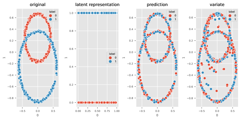
Figure 5.4: 1D example

We repeat this experiment with random circles for a bimodal Gaussian distribution with modes centered at $-5$ and $5$. The first graph shows the original distribution, the second one is the representation of the distribution in 1-dimensional latent space, the third graph is the reconstruction of the original bimodal distribution, and the fourth graph is the reconstruction on unseen latent variables.

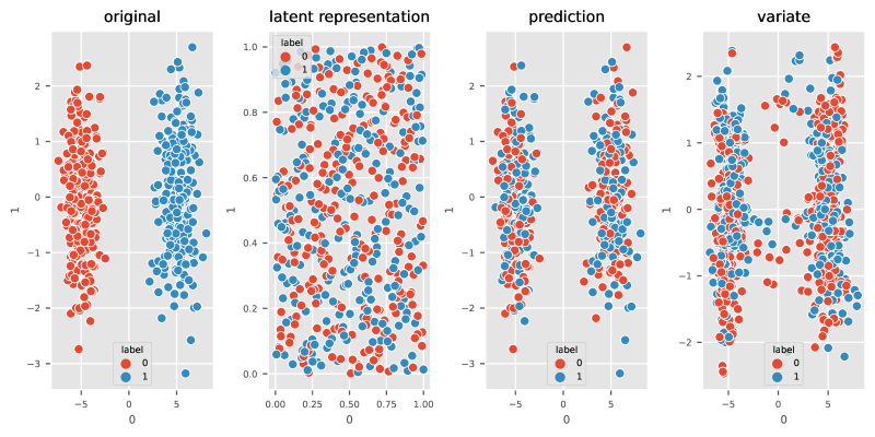
Figure 5.5: 2D example

We observe a perfect reconstruction using latent training data, and some aberrations on unseen latent variables.

Next, we repeat the experiment for a two-dimensional case. Figure 5.6 compares the distributions of $X\in\mathbb{R}^{1000\times 2}$ and $Y\in\mathbb{R}^{1000\times 2}$ (original and computed distribution), with the first scatter plot comparing to a Gaussian, second to a $t-$distribution, and the third and fourth scatter plots showing a bimodal Gaussian and $t-$distribution respectively with $N_{x}=N_{y}=1000$.

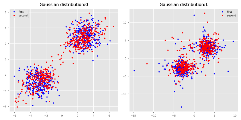
Figure 5.6: 2D Gaussian vs sampled (left) and 2D Student’s t distribution vs sampled (center) and 2D bimodal Gaussian vs sampled (right)

Table 5.13 in the Appendix to this chapter presents the first four moments of the true and sampled distributions. The sampling algorithm cannot capture the fourth moment for a heavy-tailed unimodal distribution, where we chose a degree of freedom $df=3$ for the $t$-distribution. However, it can capture the third and fourth moments of light and heavy-tailed distributions, but Figure 5.6 shows that there are some samples between the two modes.

Higher dimensional illustrations

The next two plots display a bimodal Gaussian distribution in dimension $D=15$ and resampled random variables using the optimal transport and parametric representation algorithm, respectively.

5.3.2 Conditioned random variables

Let $\mathbb{X}\in\mathbb{R}^{D_{X}},\mathbb{Y}\in\mathbb{R}^{D_{Y}}$ two dependent random variables and consider $\mathbb{Z}=\Big{(}\mathbb{X},\ \mathbb{Y}\Big{)}\in\mathbb{R}^{D_{X}+D_{Y}}$ the joint random variable. Let $Z=(X,Y)\in\mathbb{R}^{N,D_{x}+D_{y}}$ a variate of $\mathbb{Z}$, we propose a generative approach to model the conditioned random variable

$$\mathbb{Y}|\mathbb{X}.$$ (5.3.2)

Suppose known a variate of the joint variable $Z=\Big{(}X,Y\Big{)}=(z^{n})_{n=1\ldots N}$, $z^{n}=(x^{n},y^{n})$. Consider another distribution $\epsilon=(\epsilon^{n})_{n=1\ldots N}$, for instance a uniform one, and define the encoding map

$$\mathcal{L}(X,\epsilon)\text{ satisfying }\mathcal{L}(x^{n},\epsilon^{n})=x^{\sigma(n)},y^{\sigma(n)}.$$

Note that the latent variable is here the inner product $(x^{n},\epsilon^{n})_{n=0,\ldots}$. We emphasize that, in the previous formulation, the latent variable $\epsilon$ can be any draw from any distributions. In particular, one can consider $\epsilon=\mathbb{Y}$, leading to a trivial permutation $\sigma(n)=n$, a choice that can be handy in some situations to fasten computations.

Using this encoding map, we can now estimate quickly any conditioning (5.3.2). For instance, a generator of $\mathbb{Y}|\mathbb{X}=x$ can be expressed as the following map

$$\mathbb{Y}\ |\ \mathbb{X}=x\sim\mathcal{L}(x,\epsilon)$$ (5.3.3)

This approach, by defining a continuous, invertible mapping, from the latent distribution $(\mathbb{X},\epsilon)$ to the target distributions $(\mathbb{X},\mathbb{Y})$, can be helpful in a number of situations, and serve purposes beyond estimating conditioned distributions.

However, we can benchmark its results with alternative methods to compute conditional distributions, and we describe succinctly in the following two of them, that we use to benchmark our generative algorithm.

The first one is the Nadaraya-Watson kernel regression introduced in 1964 in [45]. This algorithm applies to any conditional probability according to the following formula:

$$p(y|x)\sim\frac{\sum_{i=1}^{N}K(x,x^{i})K(y,y^{i})}{\sum_{i=1}^{N}K(x,x^{i})}.$$ (5.3.4)

This is implemented in our framework as the function $kernel\_density\_estimator(...)$. This probability density can be used with a rejection sampling algorithm to provide a generator.

The second one is given by the mixture density networs, which is a quite similar strategy and models conditional probabilities

$$p(y|x)\sim\sum_{i=1}^{N}\pi_{k}(x,\omega)\mathcal{N}\Big{(}y|\mu_{k}(x,\omega),\sigma^{k}(x,\omega)\Big{)},$$ (5.3.5)

where $\omega$ are the weights of the networks. We used the framework tensorflow probability, where weights are calibrated minimizing the log likelihood loss function to a given distribution.

Example: Log-normal distributions. We illustrate our approach with a one-dimensional, nonlinear combination of variates. Consider two independent distributions $\mathbb{X},\mathbb{Y}$, having normal distribution $\mathcal{N}(\mu_{x},\sigma_{x})$ and $\mathcal{N}(\mu_{y},\sigma_{y})$, with $(\mu_{x},\mu_{y})=(0,0)$, $(\sigma_{x},\sigma_{y})=(1,0.1)$, and consider the following distribution:

$$\mathbb{Z}:=\Big{(}\exp(\mathbb{X}),\exp(\mathbb{X})\exp(\mathbb{Y}))\Big{)}.$$

In Figure 5.7-(i), we plot in red a variate of the joint distribution $(\mathbb{X},\mathbb{Y})$ of size $N=1000$. We conditioned upon $x=0$, and we plot in blue a sample of the conditioned variate $\mathbb{Y}\ |\ \mathbb{X}=0$. This blue distribution serves us as reference target distribution.

Figure 5.7-(ii) shows the density of the conditioned random variable algorithm in blue, against the reference target distribution, where the estimator is the Nadaraya Watson one (5.3.4). We used in this benchmarks a particular kernel, called the inverse quadratic kernel, corresponding to a Cauchy distribution, defined as $K(x,y)=\frac{\pi}{1+|x-y|^{2}}$. This kernel is used together with a scaling map $S(x)=\frac{x}{h}$, $h$ being the bandwidth, that has been set manually by trial and error to the value $h=0.04$ in our example.

Figure 5.7-(iii) uses the same kernel, together with the generative method (5.3.2). Here the latent variable is taken to be the marginal $Y$.

Figure 5.7-(iv) uses the same kernel, together with the generative method (5.3.2). Here the latent variable is taken to be a standard gaussian variable.

Figure 5.7-(v) uses the Gaussian mixture (5.3.2).

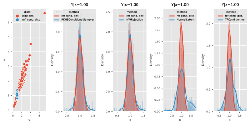
Figure 5.7: A benchmark of conditionned algorithm for log-normal distributions

Table 5.15 performs also statistical tests of both methods against the reference target distribution. We then repeat the same experience, but moving the conditioning value to $x=2$, and display the statistical test in Table 5.16.

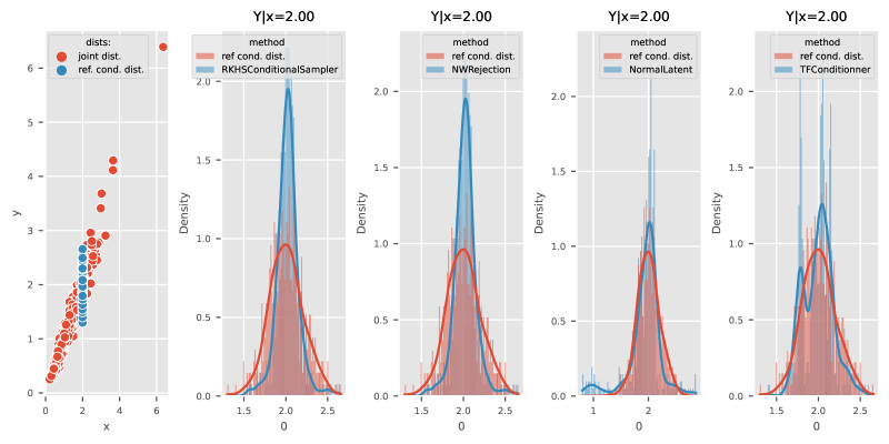
Figure 5.8: A benchmark of conditionned algorithm for log-normal distributions

Analysis

As illustrated by the above example, both kernel methods (ii) and (iii) give very similar results, when used in the very same experimental conditions, that is if they share the same kernel $k$, and also a distribution, that is used for the rejection algorithm, as well as the latent distribution $\epsilon$ in (5.3.3). The generative method (5.3.3) produces then distributions having the same probability density than the Nadaraya Watson estimator. However, the Nadaraya Watson estimator, coupled with the rejection sampling method, is more computationally efficient.

Observe that there is an added degree of freedom for generative methods (5.3.3), that is the choice of the latent distribution. This distribution can be any distribution, for instance a uniform one. This freedom allows to design generative methods that are accurate enough, somehow “swiss-knife” as they give satisfactory results in a large number of situations, avoiding some difficulties, as picking up a kernel dedicated to a given conditioning, or selecting good prior for the rejection algorithm, that can be cumbersome for complex distributions.

5.4 Two useful applications of generative methods

5.4.1 Transition probability algorithms

Motivation. We now propose a general Python interface to a function computing conditional expectations problems in arbitrary dimensions, that we named Pi. We also propose a kernel-based implementation of these problems, which is described in [31] and [33].

Benchmarking such algorithms is a difficult task, as the literature did not provide competitor algorithms to compute conditional expectations to kernel-based methods, for arbitrary dimensions, to our knowledge. Indeed, these algorithms are tightly concerned with the so called curse of dimensionality, as we are dealing with arbitrary dimensions algorithms.

However, there is a recent, but impressively fast-growing, literature, devoted to the study of machine learning methods, particularly in the mathematical finance applications, see [17] and ref. therein for instance. In particular, a neural networks approach has been proposed to compute conditional expectation in [22] that we can use as benchmark.

The Pi function. Consider any martingale process $t\mapsto X(t)$, and any positive definite kernel $k$, we define the operator $\Pi$ (using Python notations)

$$f_{Z|X}=\Pi(X,Z,f(Z))$$ (5.4.1)

where

• $X\in\mathbb{R}^{N_{x},D_{X}}$ is any set of points generated by a i.i.d sample of $X(t^{1})$ where $t^{1}$ is any time.

• $Y\in\mathbb{R}^{N_{Y},D_{Y}}$ is any set of points, generated by a i.i.d sample of $X(t^{2})$ at any time $t^{2}>t^{1}$.

• $f(Y)\in\mathbb{R}^{N_{Y},D_{f}}$ is any, optional, function.

The output is a matrix $f_{Z|X}$, representing the conditional expectation

$$f_{Z|X}\sim\mathbb{E}^{X(t^{2})}(f(\cdot)|X(t^{1}))\in\mathbb{R}^{N_{x},D_{f}}=:^{not.}f(Z|X).$$ (5.4.2)

• if $f(Z)$ is let empty, the output $f_{Z|X}\in\mathbb{R}^{N_{z},N_{x}}$ is a matrix, representing a convergent approximation of the stochastic matrix $\mathbb{E}^{X(t^{1})}(Z|X)$.

• if $f(Z)\in\mathbb{R}^{N_{z},D_{f}}$ is not empty, $f_{Z|X}\in\mathbb{R}^{N_{z},D_{f}}$ is a matrix, representing the conditional expectation $f(Z|X)=\mathbb{E}^{X(t^{1})}(f(Z)|X)$.

5.4.2 Sum of random variables

Next, we consider two independent random variables $\mathbb{X},\mathbb{Y}$, and propose some algorithms to solve the transport equation $S_{\#}(d\mathbb{X})=d\Big{(}\mathbb{X}+\mathbb{Y}\Big{)}$. This kind of situation is of interest, for instance for PDE methods, where solutions of numerous problems can be written as $\mathbb{X}^{n+1}=\mathbb{X}^{n}+\mathbb{Y}^{n}$, $\mathbb{Y}^{n}$ being the distribution of a Green function.

We recall that the sum of two random variables $\mathbb{X}+\mathbb{Y}$, having density $d\mathbb{X},d\mathbb{Y}$, is a random variable having density $d\left(\mathbb{X}+\mathbb{Y}\right)=d\mathbb{X}\ast d\mathbb{Y}$, $\ast$ being the convolution. According to the definition of transport maps (5.1.4), taking into account the definition of convolution, this paragraph aims to find a smooth, invertible map $S$ such that for any continuous function $\varphi$,

$$<\varphi,d\mathbb{X}\ast d\mathbb{Y}>=\int\int\varphi(x+y)d\mathbb{X}(x)d\mathbb{Y}(y)=\int(\varphi\circ S)d\mathbb{X}$$

Let us focus on the discrete case from now on. Consider $X=(x^{1},\ldots,x^{N_{X}})$, $Y=(y^{1},\ldots,y^{N_{Y}})$ and denote $d\mathbb{X}_{X}=\frac{1}{N_{X}}\sum_{n=1}^{N_{X}}\delta_{x^{n}}$, $d\mathbb{Y}_{Y}=\frac{1}{N_{Y}}\sum_{n=1}^{N_{Y}}\delta_{y^{n}}$, $X+Y=(x^{n}+y^{m})_{n,m=1}^{N_{X},N_{Y}}$. Then

$$d\mathbb{X}_{X}\ast d\mathbb{Y}_{Y}=\frac{1}{N_{X}\times N_{Y}}\sum_{n,m=1}^{N_{X},N_{Y}}\delta_{x^{n}+y^{m}}$$

Observe that $d\mathbb{X}_{X}\ast d\mathbb{Y}_{Y}$ is a distribution having $N_{X}\times N_{Y}$ elements, since we want to map it to a distribution $X$ having $N_{X}$ elements. A possibility to solve this problem is to consider the clustering approach (4.3.4), that is

$$\inf_{Z\in\mathbb{R}^{N_{X},D}}D_{k}(\mathbb{X}_{X}+\mathbb{Y}_{Y},\mathbb{Z}_{Z})$$

Then consider the map defined as $S_{\#}d\mathbb{X}_{X}=d\mathbb{Z}_{Z}$ defined at (5.1.10). However, this approach is computationally costly, and generative methods allow one to design more performing algorithms, as follows.

Consider any two independent latent variables $\mathbb{X},\mathbb{Y}$ and $\epsilon_{x},\epsilon_{y}$, for instance uniform laws, and definethe two encoders

$$\mathbb{X}=\mathcal{L}_{x}(\epsilon_{x}),\quad\mathbb{Y}=\mathcal{L}_{y}(\epsilon_{y}).$$ (5.4.3)

In this setting, a generator of the sum $\mathbb{X}+\mathbb{Y}$ is simply

$$\mathbb{X}+\mathbb{Y}=\mathcal{L}_{x}(\epsilon_{x})+\mathcal{L}_{y}(\epsilon_{y}).$$

We illustrate this approach with a simple example: Consider two independent normal distribution $d\mathbb{X}=\mathcal{N}(\mu_{x},\sigma_{x})$ and $d\mathbb{Y}=\mathcal{N}(\mu_{y},\sigma_{y})$, and consider the sum

$$\mathbb{Z}=\mathbb{X}+\mathbb{Y},\quad d\mathbb{Z}=d\mathbb{X}\ast d\mathbb{Y}=\mathcal{N}(\mu_{x}+\mu_{y},\sqrt{\sigma_{x}^{2}+\sigma_{x}^{2})},$$

and $d\mathbb{Z}$ can be used as a reference distribution for benchmarks. We consider the generative approach (5.4.3), taking as latent variable $(\epsilon_{x},\epsilon_{y})$ the uniform distribution over the unit square $[0,1]^{2}$. The result is plot figure 5.9, where the first figure plot the two variates of the distributions $d\mathbb{X},d\mathbb{Y}$ in the first subplot. The second subplot 5.9-(ii) represent the reference distribution $d\mathbb{Z}$, together with the result of the generative approach (5.4.3).

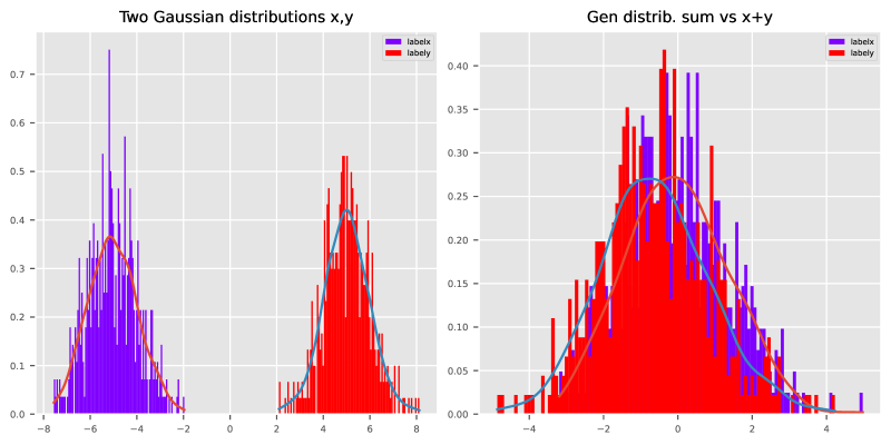
Figure 5.9: Bivariate Gaussian and student’s t distribution

Table 5.11 displays statistical tests to compare the generated distribution $\mathcal{L}_{x}(\epsilon_{x})+\mathcal{L}_{y}(\epsilon_{y})$ against the reference distribution $d\mathbb{Z}$.

Table 5.11: Stats

	0
Mean	-0.026(-0.62)
Variance	0.2(0.19)
Skewness	1.9(2.1)
Kurtosis	-0.18(0.18)
KS test	1.8e-08(0.05)

5.5 Appendix to Chapter 4

1D distributions. Table 5.12 illustrates the skewness, the kurtosis between $X\in\mathbb{R}^{1000\times 1}$ and $Y\in\mathbb{R}^{1000\times 1}$ for the Gaussian and Student’s $t-$distributions from Section 5.3.1.

Table 5.12: Stats

	Mean	Variance	Skewness	Kurtosis	KS test
Gaussian distribution	-0.018(0.17)	0.0052(0.065)	10(12)	-1.6(-1.3)	0.042(0.05)
t-distribution	0.023(0.17)	0.033(0.065)	12(12)	-1.2(-1.3)	0.72(0.05)

2D distributions. To check numerically some first properties of the generated distribution, We output in Table 5.13 the skewness and kurtosis, probability distances of both $X\in\mathbb{R}^{1000,2}$ and $Y\in\mathbb{R}^{1000,2}$. Each row represents the truth distribution $X$ and generated distribution using a sampling function labeled as “sampled” $Y$:

Table 5.13: Summary statistics

	Mean	Variance	Skewness	Kurtosis	KS test
Gaussian distribution:0	0.0039(0.18)	-0.00068(-0.11)	9.8(11)	-1.6(-1)	0.23(0.05)
Gaussian distribution:1	0.025(0.4)	0.015(0.13)	9.9(11)	-1.6(-0.89)	0.095(0.05)
t-distribution:0	0.025(0.18)	-0.13(-0.11)	13(11)	-0.69(-1)	0.059(0.05)
t-distribution:1	0.045(0.4)	-0.041(0.13)	12(11)	-0.62(-0.89)	0.024(0.05)

15D encoders. Table 5.14 illustrates the skewness, the kurtosis between $X\in\mathbb{R}^{500\times 15}$ and $Y\in\mathbb{R}^{500\times 15}$ for the Gaussian and Student’s $t-$ bi-modal distributions from Section 5.3.1.

Table 5.14: Stats

	Mean	Variance	Skewness	Kurtosis	KS test
Optimal transport (Max)	-0.011(-0.01)	-0.011(-0.058)	10(2.9)	-1.6(-0.037)	5.6e-14(0.05)
Optimal transport (Median)	-0.0055(0.079)	0.023(-0.047)	9.4(2.5)	-1.6(0.22)	1.5e-14(0.05)
Optimal transport (Min)	-0.057(0.028)	-0.031(-0.17)	11(2.9)	-1.6(-0.1)	2.4e-17(0.05)
Param. represent. (Max)	-0.048(0.023)	-0.012(0.068)	9.9(8.8)	-1.6(-1.4)	0.25(0.05)
Param. represent. (Median)	0.039(0.075)	-0.03(-0.042)	9.9(7.9)	-1.6(-1.5)	0.15(0.05)
Param. represent. (Min)	0.028(0.18)	0.042(0.023)	9.6(7.2)	-1.6(-1.5)	0.012(0.05)

Conditioned random variables

The following table summarizes statistics for the numerical experiment in Section 5.3.2, with a conditioned variable $\mathbb{Y}\ |\ \mathbb{X}=1$.

Table 5.15: Stats

	Mean	Variance	Skewness	Kurtosis	KS test
RKHSConditionalSampler	1(1)	0.18(0.31)	0.0096(0.019)	-0.24(3)	0.26(0.05)
NWRejection	1(1)	0.18(0.31)	0.0096(0.019)	-0.24(3)	0.26(0.05)
NormalLatent	1(1)	0.18(0.14)	0.0096(0.074)	-0.24(1.1)	7e-10(0.05)
TFConditionner	1(1)	0.18(0.1)	0.0096(0.04)	-0.24(0.89)	1.9e-10(0.05)

This table summarizes statistics for the second numerical experiment in Section 5.3.2, with a conditioned variable $\mathbb{Y}\ |\ \mathbb{X}=2$.

Table 5.16: Stats

	Mean	Variance	Skewness	Kurtosis	KS test
RKHSConditionalSampler	2(2)	0.097(0.4)	0.042(0.018)	0.22(3.6)	5.7e-08(0.05)
NWRejection	2(2)	0.097(0.4)	0.042(0.018)	0.22(3.6)	5.7e-08(0.05)
NormalLatent	2(1.9)	0.097(-1.3)	0.042(0.096)	0.22(4)	1e-05(0.05)
TFConditionner	2(2)	0.097(0.15)	0.042(0.031)	0.22(-0.01)	0.011(0.05)

5.6 Bibliography

Many implementations of LSAP are available in a Python interface. For example, in Scipy, the optimization and root finding module allows one to find LSAP using a Hungarian algorithm when the cost matrix is unbalanced. A Python library Lapjv allows one to find LSAP using Jonker-Volgenant algorithm. The Sinkhorn algorithm, is (heuristically) fast for the Kantorovich problem and solve LSAP efficiently, but the matrix based on the Sinkhorn algorithm is not always a permutation matrix. In certain settings, it was implemented in POT library.

Chapter 6 Application to partial differential equations

6.1 Introduction

We now explore how kernel methods can be applied to solve partial differential equations (PDEs), and we demonstrate here that the mapproach we propose offers some advantages over traditional numerical methods for PDEs.

• Meshless methods. Kernel methods allow for meshless (sometimes called meshfree) formulations to be used. Unlike traditional finite difference or finite element methods, meshless methods do not require a predefined mesh, nor to compute connections between nodes of the grid points. Instead, they use a set of nodes or particles to represent the domain. This makes them particularly useful for modeling complex geometric domains.

• Particle methods. Kernel methods can be used in the context of particle methods in fluid dynamics, which are Lagrangian methods involving the tracking of the motion of particles. Kernel methods are well-suited for these types of problems because they can easily handle general meshes and boundaries.

• Boundary conditions. Indeed Kernel methods allow one to express complex boundary conditions, which can be of Dirichlet or Neumann type, or even of more complex mixed-type expressed on a set of points. They also can also encompass free boundary conditions for particle methods, as well as fixed meshes.

We are going to provide several illustrations of the flexibility of this approach. The price to pay with meshless methods is the computational time, which is greater than the one in more traditional methods such as finite difference, finite element, or finite volume schemes. The reason is that kernel methods usually produces dense matrix, whereas more classical methods on structured grids, due to their localization properties, typically lead to sparse matrix, a property that matrix solvers can benefit on.

In this chapter, we initiate our discussion with some of the technical details pertinent to the discretization of partial differential equations via kernel methods. Building on this material, we then present a series of examples, commencing with static models and progressing to encompass a spectrum of time evolution equations. Our primary goal is to showcase and the efficacy and broad applicability of meshfree methods, in the context of, both, structured and unstructured meshes.

6.2 Kernel approximation techniques

6.2.1 Kernel-based operators

We discuss some aspects related to consistency of differential operators introduced in Section 4.2. We start discussing the consistency of the divergence operator (4.2.5) as an example, that we rewrite here in its extrapolation version: given a set of distinct points $X\in\mathbb{R}^{N_{x},D}$, consider the measure $d\mathbb{X}:=\sum_{n=1}^{N_{x}}\frac{1}{N_{x}}\delta_{x^{n}}$, then this operator is defined for any points $z$ as

$$z\mapsto\nabla_{k}(X,z)^{T}=K(X,X)^{-T}\Big{(}\nabla_{z}K\Big{)}(z,X)^{T}\in\mathbb{R}^{N_{x},D},$$ (6.2.1)

This operator acts on any (sufficiently regular) vector-field function $\phi(X)\in\mathbb{R}^{N_{x},D}$, as the Frobenius scalar product $\nabla_{k}(X,z)^{T}\cdot\phi(X)$, to compute an approximation of the divergence of the vector-field $\phi$. In particular, one can estimate this operator on all points of the set $X$. We compute that, for any scalar field $\varphi$, this operator acts as

$$<\varphi(X),\nabla_{k}(X,X)^{T}\cdot\phi(X)>\quad\text{ for all }\phi,\varphi,$$

where $\nabla_{k}(X,X)\in\mathbb{R}^{N_{X},D,N_{x}}$ is now a three-tensor, $\phi(X)\in\mathbb{R}^{N_{X},D}$ is a matrix, $\varphi(X)\in\mathbb{R}^{N_{X}}$ is a scalar field, and $\cdot$ means here a contraction on the first two indices. So we can rewrite this latter formula as

$$<\varphi(X),\nabla_{k}(X,X)^{T}\cdot\phi(X)>=<\nabla_{k}(X,X)\varphi(X)\ ,\phi(X)>=<\phi(\cdot)d\mathbb{X}\ ,\nabla_{k}\varphi(\cdot)>_{\mathcal{D}^{\prime},\mathcal{D}}.$$

where now the right side of the equation above denote the weak topology on distributions. In particular, assume that the discretized operator $(\nabla_{k}\varphi)(X)$ is consistent with $(\nabla\varphi)(X)$ at the set of point $X$ for any functions belonging to $\varphi\in\mathcal{H}_{k}^{X}$, the kernel space induced by $k$. Then, our operator $\nabla_{k}^{T}$ is consistent with the operator

$$\big{(}\nabla_{k}^{T}\cdot\phi\big{)}(X)\simeq-\nabla\cdot(\phi\,d\mathbb{X}),$$

So one should pay attention to the fact that the operator $\nabla_{k}^{T}$, that is the transpose of the gradient operator $\nabla_{k}$, is not consistent with the divergence operator $\nabla\cdot\phi$, but with the weighted operator $-\nabla\cdot(\phi d\mathbb{X})$. If the “true” divergence operator is needed, it can be built straightforwardly from the operator $\nabla_{k}$. In the same way, the operator $\Delta_{k}$ introduced in (4.2.6) is not consistent with the “genuine” Laplace operator $\Delta=\sum_{i=1}^{D}\partial_{i}^{2}$, but is instead consistent with the weighted operator

$$\Delta_{k}\varphi\simeq-\nabla\cdot(\nabla\varphi\,d\mathbb{X}).$$

6.2.2 Time-evolution operators based on $\theta$-schemes

When it comes to discretization of time-evoluting PDEs, the approach used in this book usually resumes to consider the following class of dynamical system with Cauchy initial conditions

$$\frac{d}{dt}u(t)=Au(t),\quad u(0)\in\mathbb{R}^{N_{X},D},\quad A\in\mathbb{R}^{N_{X},N_{X}},$$ (6.2.2)

where $A\equiv A(t,x,u,\nabla u)$ can be any matrix valued operator, assumed to be negative defined, i.e. satisfying

$$<Au,u>\leq 0\qquad\text{ for all }u\in\mathbb{R}^{N_{X}}.$$

Thus we follow a quite classical way to deal with such a dynamical system.

Let $\ldots<t^{n}<t^{n+1}<\ldots$ be a time discretization, and $\tau^{n}=t^{n+1}-t^{n}$. For a given parameter $0\leq\theta\leq 1$, the following discretization is referred to as a $\theta$-scheme:

$$\delta_{t}u(t^{n})=\frac{u(t^{n+1})-u(t^{n})}{t^{n+1}-t^{n}}=A\Big{(}\theta u(t^{n+1})+(1-\theta)u(t^{n})\Big{)}=Au^{\theta}(t^{n}).$$

A formal solution of this scheme is given by $u(t^{n+1})=B(A,\theta,dt)u(t^{n})$, where $B$ is the generator of the equation, defined as

$$B(A,\theta,\tau^{n})=\Big{(}I-\tau^{n}\theta A\Big{)}^{-1}\Big{(}I+\tau^{n}(1-\theta)A\Big{)}.$$ (6.2.3)

• The value $\theta=1$ corresponds to the implicit approximation.

• The value $\theta=0$ corresponds to the explicit approximation.

• The value $\theta=0.5$ corresponds to the Crank Nicolson choice.

The Crank Nicolson choice is motivated by the following energy estimate, taking the scalar product with $u^{\theta}(t^{n})$ in the discrete equation ($\ell^{)}$ denoted the standard discrete quadratic norm)

$$<Au^{\theta}(t^{n}),u^{\theta}(t^{n})>_{\ell^{2}}=\frac{\theta\|u(t^{n+1})\|_{\ell^{2}}^{2}-(1-\theta)\|u(t^{n})\|_{\ell^{2}}^{2}+(1-2\theta)<u(t^{n+1}),u^{\theta}(t^{n})>_{\ell^{2}}}{\tau^{n}}.$$

For $\theta\geq 0.5$, an energy dissipation $\|u(t^{n+1})\|_{\ell^{2}}^{2}\leq\|u(t^{n})\|_{\ell^{2}}^{2}$ is achieved, provided $A$ is a negative defined operator. Choosing $\theta\geq 0.5$ leads to unconditionally stable and convergent numerical schemes. The Crank Nicolson choice $\theta=0.5$ is a swiss-knife choice, that is much adapted to energy conservation, that is considering operators $A$ satisfying $<Au,u>_{\ell^{2}}=0$.

The python function $alg.CrankNicolson(A,dt,u^{0}=[],\theta)$ outputs

• either $u(t^{n+1})$ if $u^{0}=u(t^{n})$ is input.

• or $B(A,\theta,dt)$ if $u^{0}$ is not.

6.2.3 Entropy dissipative schemes

We now extend the $\theta$-scheme framework to general, high-order, multi-time steps entropy dissipative schemes, applicable to various scenarios discussed in this monograph. The approach is based on ([27] and references therein) in the context of finite-difference, one-by schemes, and is extended here to multi-dimensional systems modeled using the RKHS framework of this monograph. The systems of interest satisfy Hamilton-Jacobi-type equations in a weak sense:

$$\partial_{t}u(t,x)=\nabla_{x}\cdot f(t,u,\nabla_{x}u,\ldots),\quad u(0,x)\in\mathbb{R}^{D_{u}}\text{ prescribed},x\in\mathbb{R}^{D_{x}}$$ (6.2.4)

where $\nabla\cdot$ represents the divergence, and $f(t,u,\ldots)\in\mathbb{R}^{D_{x},D_{u}}$ is a matrix field. For instance, $f(t,u,\ldots)\equiv v(t,x)u$ corresponds to a transport equation, while $f(t,u,\ldots)=\nabla_{x}u$ leads to the heat equation $\partial_{t}u=\Delta u$. Hamilton-Jacobi equations are thus applicable to hyperbolic-diffusive models. Consider a scalar-valued, entropy function $U=U(u)$, and denote the entropy variable $v(u)=\nabla_{u}U(u)$. We assume the existence of a vector-valued map $v\mapsto g(v)$ and a scalar-valued function $v\mapsto G(v)$, allowing the equations (6.2.4) to be written with an entropy dissipation term:

$$\partial_{t}u+\nabla_{x}\cdot g(v(u))=0,\quad\partial_{t}U(u)+\nabla_{x}\cdot G(v(u))\leq 0.$$ (6.2.5)

The entropy dissipation must also be understood in a weak sense. In particular, (6.2.5) implies the bound

$$\frac{d}{dt}\int_{\mathbb{R}^{D_{x}}}U(u(t,x))\,dx\leq 0$$

for any solution to (6.2.4)-(6.2.5). In turn, this implies the $L^{p}$-stability of a solution (if available), provided the entropy function $U$ is convex.

To approximate such a system numerically, we consider a positive definite kernel $k$, a time grid $\ldots<t^{n}<t^{n+1}<\ldots$, a space grid $X=(x^{1},\ldots,x^{N_{x}})\in\mathbb{R}^{N_{x},D_{x}}$, and we denote by $\tau^{n}=t^{n+1}-t^{n}$, $u_{i}^{n}\sim u(t^{n},x^{i})$ the discrete solution, and by $\delta_{t}U^{n}=\frac{U^{n+1}-U^{n}}{\tau^{n}}$. The strategy for building entropy dissipative schemes involves first the choice of a $(q+1)$-time level interpolation $u^{*}(u^{q},..,u^{0})$ which should satisfy:

• Consistency with the identity $(u^{*}(u,..,u)=u)$.

• Invertibility and regularity of the map $u^{q}\rightarrow u^{*}(u^{q},..,u^{0})$.

To build this time-integrator operator, we can for instance solve in $\beta^{n}=(\beta^{n,p})_{p=0}^{q}$ the following Van der Monde system (see Appendix 6.6.1 for a justification):

$$A^{n}\beta^{n}=(1,0,\ldots,0)^{T},\quad A^{n}=(a_{i,j}^{n})_{i,j=0}^{q},\quad a_{i,j}^{n}=\Big{(}t^{*n}-t^{n-j}\Big{)}^{j}$$ (6.2.6)

for some $t^{n}\leq t^{*}\leq t^{n+1}$, and set $u^{*}(u^{q},..,u^{0})=\sum_{p=0}^{q}\beta^{n,p}u^{n-p}$. Indeed, there exist $t^{n}\leq t^{*}\leq t^{n+1}$ such that this operator is of order $q+2$. (See [27].)

Let $u^{*,n}=u^{*}(u^{n},..,u^{n-q})$, and let us choose the entropy variable $U^{*}(u^{q},..,u^{0})$, with $U(u^{*})$ as a possible choice. We set $U^{*,n}=U^{*}(u^{n},..,u^{n-q})$. This variable must enjoy the following:

• Be consistent with the original entropy $U(u)$ (i.e. $U^{*}(u,..,u)=U(u)$).

• Define the $(q+2)$-time entropy variable $v^{*,n+1/2}(u^{q+1},..,u^{0})$, which satisfies

  $$\delta_{t}U^{*,n}=\frac{U^{*,n+1}-U^{*,n}}{\tau^{n}}=v^{*,n+1/2}\cdot\delta_{t}u^{*,n}$$

  
  

  and is consistent with the entropy variable : $v^{*,n+1/2}(u,..,u)=v(u)$.

The system is then approximated by the fully discrete numerical scheme displayed now, where $u^{n+1}$ is the unknown:

$$\delta_{t}u^{*,n}=\frac{u^{*,n+1}-u^{*,n}}{\tau^{n}}=-\nabla_{k}\cdot g(v^{*,n+1/2}).$$ (6.2.7)

These schemes can be fully implicit or explicit with respect to the unknown $u^{n+1}$, based on the entropy variable choice. They are entropy stable as follows: set $E^{*,n}=\sum_{i=1}^{N_{x}}U(u_{i}^{n})$ and compute

$$\delta_{t}E^{*,n}=\sum_{i}\nabla_{k}\cdot G(v_{i}^{*,n+1/2})=<G(v^{*,n+1/2}),\nabla_{k}1>_{\ell^{2}}.$$

If we consider a kernel and defines a divergence operator that satisfies $\nabla_{k}1\equiv 0$, then the numerical scheme (6.2.7) is stable, as it enjoyes the property $E^{*,n+1}\leq E^{*,n}$. For instance, consider the linear equation (3.2.4), the scheme $\delta_{t}u^{n}=Av^{*,n+1/2}$ with $v^{*,n+1/2}=\frac{u^{n+1}+u^{n}}{2}$, and the entropy function $U(u)=u^{2}$. We can directly compute that $\delta_{t}U(u^{n})=v^{*,n+1/2}Av^{*,n+1/2}\leq 0$. The Crank-Nicolson choice $\theta=1/2$ corresponds to a two-time level, entropy scheme, which is second-order accurate in time.

6.3 Solving a few standard PDEs

6.3.1 Poisson equation

We start our numerical illustration solving the Laplace operator on a fixed domain. Suppose that we want to solve the following Poisson equation with Dirichlet conditions

$$\Delta u=f,\quad\text{ supp }u\subset\Omega,\quad u_{\partial\Omega}=0,$$

where $f$ is sufficient regular and $\Omega$ is a sufficient regular domain. Consider the weak formulation of this equation, that is for functions $\varphi$ supported in $\Omega$

$$<\Delta u,\varphi>_{\mathcal{D}^{\prime},\mathcal{D}}=-<\nabla u,\nabla\varphi>_{\mathcal{D}^{\prime},\mathcal{D}}=\int_{\mathbb{R}^{D}}(f\varphi)(x)dx.$$

To compute an approximation of this equation with a kernel method we proceed as follows:

• Select a mesh $X\in\mathbb{R}^{N_{x},D}$ representing $\Omega$.

• Choose a kernel $k$ that generates a space of null trace functions.

A kernel approximation of this equation consists in approximating the solution as a function $u\in\mathcal{H}_{k}^{X}$, that is the finite dimensional kernel Hilbert Space generated by the kernel $k$ and the set of points $X$, satisfying

$$<\nabla_{k}u,\nabla_{k}\varphi>_{\mathcal{H}_{k}^{X}}=-<\Delta_{k}u,\varphi>_{\mathcal{H}_{k}^{X}}=<f,\varphi>_{\mathcal{H}_{k}^{X}}\quad\text{ for all }\varphi\in\mathcal{H}_{k}^{X},$$

leading to the equation $(\Delta_{k}u)(X)=f(X)$, $\Delta_{k}$ being defined in (4.2.6). A solution to this equation is computed as $u=(\Delta_{k})^{-1}f$, defined in (4.2.7).

Figure 6.1 displays a regular mesh for the domain $\Omega=[0,1]^{2}$, where $f$ is plotted in the left=hand side, and the solution $u$ in the right=hand side.

Figure 6.1: Computed inverse Laplace operator - regular mesh

Kernel methods facilitate the use of unstructured meshes, enabling the description of more complex geometries. Figure 6.2 shows an unstructured mesh generated by a bimodal Gaussian, with $f$ plotted on the left and the solution $u$ on the right.

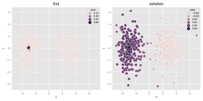
Figure 6.2: Computed inverse Laplace operator - irregular mesh

6.3.2 A denoising problem

We now emphasize the optional regularization term in the projection operator (3.3.1), introduced as an additional parameter in the pseudo-inverse formula (3.2.3).

Suppose we want to solve a minimization problem of the form:

$$\inf_{G\in{\mathcal{H}}_{k}(\mathcal{X})}\|G-F\|_{\mathcal{H}_{k}(\mathcal{X})}^{2}+\epsilon\|L(G)\|_{L^{2}(\mathcal{X})}^{2}$$

Here, $L:\mathcal{H}_{k}(\Omega)\mapsto L^{2}(\Omega)$ is a linear operator that serves as a penalty term. A formal solution is given by:

$$G+\epsilon L^{T}LG=F$$

Numerically, consider $X\in\mathbb{R}^{N_{x},D}$ a variate of $\mathbb{X}$, defining an unstructured mesh $\mathcal{X}$, together with a kernel $k$ for defining $\mathcal{H}(\mathcal{X})$. Denote $L_{k}$ the discretized operator. This penalty problem defines a function $G$ as follows:

$$z\mapsto G(z)=K(X,z)\Big{(}K(X,X)+\epsilon\Big{(}L_{k}^{T}L_{k}\Big{)}(X,X)\Big{)}^{-1}F(X)$$

To compute this function, input $R=\epsilon L_{k}^{T}L_{k}$ into the pseudo-inverse formula (3.2.3).

As an example, consider the denoiser procedure, which aims to solve:

$$\inf_{G\in\mathcal{H}_{k}(\mathcal{X})}\|G-F\|_{\mathcal{H}_{k}(\mathcal{X})}^{2}+\epsilon\|\nabla G\|_{L^{2}(\mathcal{X}))}^{2}.$$ (6.3.1)

In this case, $L_{k}=\nabla_{k}$, and $L_{k}^{T}L^{k}$ corresponds to $\Delta_{k}$. Figure 6.3 demonstrates the results of this regularization procedure. The noisy signal (left image) is given by $F_{\eta}(x)=F(x)+\eta$, where $\eta$ is a white noise, and $f$ is the cosine function defined in (3.1.2). The regularized solution is plotted on the right.

In this case, $L_{k}=\nabla_{k}$, the discrete gradient operator defined at (4.2.4), and $\nabla_{k}^{T}\nabla_{k}$ is an approximation of the operator $\Delta$. Figure 6.3 demonstrates the results of this regularization procedure. The noisy signal (left image) is given by $F_{\eta}(x)=F(x)+\eta$, where $\eta:=\mathcal{N}(0,\epsilon)$ is a white Gaussian noise, $\epsilon=0.1$, and $f(x)=f(x_{1},\ldots,x_{D})=\prod_{d=1,\ldots,D}\cos(4\pi x_{d})+\sum_{d=1,\ldots,D}x_{d}$ is a example function. The regularized solution is plotted on the right.

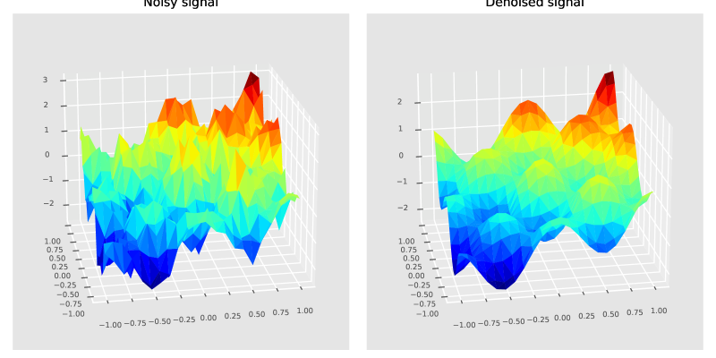
Figure 6.3: Example of denoising signals

6.4 Evolution schemes

6.4.1 A meshless Eulerian method for a fixed domain

We now investigate the numerical study of time-evolution PDEs in the context of kernel methods. We discuss their implementation within our library and provide examples. First, we introduce the $\theta$-schemes, which serve as a method for integrating time-evolution equations.

To illustrate the evolution operator (6.2.3), let’s consider the heat equation in a fixed geometry $\Omega$ with null Dirichlet conditions:

$$\partial_{t}u(t,x)=\Delta u(t,x),\quad u(0,x)=u_{0}(x),\quad x\in\Omega,\quad u_{\partial\Omega}=0$$

To approximate this equation, we follow the following steps:

• Select a mesh $X\in\mathbb{R}^{N_{x},D}$ mfor the domain $\Omega$.

• Pick up a kernel $k$ generating a space of vanishing trace functions.

We represent this equation as $\frac{d}{dt}u(t)=\Delta_{k}u(t)$, with evolution operator $u^{n+1}=B(\Delta_{k},u^{n},dt,\theta)$ and $\theta=1$. This corresponds to the fully implicit case in (6.2.3). The image 6.4 provides a 3-D representation of the initial condition and time evolution of the heat equation on a fixed square.

This approach can be easily adapted to more complex geometries, as demonstrated by the image 6.5, which shows the heat equation on an irregular mesh generated by a bimodal Gaussian process.

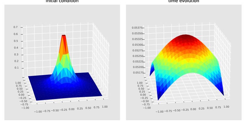
Figure 6.4: A heat equation on a fixed regular mesh

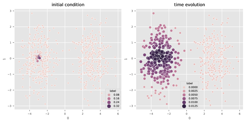
Figure 6.5: A heat equation on a irregular mesh

6.4.2 A particle method based on sharp discrepancy sequences

Next, we consider the heat equation on an unbounded domain, with measure-valued Cauchy initial data, that is:

$$\partial_{t}\mu=\Delta\mu,\quad\mu(0,x)=\mu_{0}(x),\quad x\in\mathbb{R}^{D}.$$ (6.4.1)

Instead of solving this equation on a fixed domain, we consider a Lagrangian method, that is, we compute a map, or a velocity field $y(t,x)$, transporting the initial condition to the solution. In other words, we seek a measure approximating (6.4.1) and having the form $\mu(t,\cdot)=y(t,\cdot)_{\#}\mu_{0}$. Here, we introduce an unknown map $t,x\mapsto y(t,x)$, where $x$ thought as a fixed variable. Since we are dealing with measures, the equation (6.4.1) is considered in a weak sense:

$$\frac{d}{dt}<\mu(t,\cdot),\varphi(\cdot)>_{\mathcal{D^{\prime}},\mathcal{D}}=<\mu(t,\cdot),\Delta\varphi(\cdot)>_{\mathcal{D^{\prime}},\mathcal{D}}\quad\text{ for all }\varphi\in\mathcal{C}(\mathbb{R}^{D})$$

that is, using the transport properties $\mu(t,\cdot)=y(t,\cdot)_{\#}\mu_{0}(\cdot)$ we have

$$\frac{d}{dt}<\mu_{0}(\cdot),\varphi\circ y(\cdot)>_{\mathcal{D^{\prime}},\mathcal{D}}=<\mu_{0}(\cdot),(\Delta\varphi)\circ y(\cdot)>_{\mathcal{D^{\prime}},\mathcal{D}}\quad\text{ for all }\varphi\in\mathcal{C}(\mathbb{R}^{D}).$$

We use now the expression $\Delta=\nabla\cdot\nabla$ and the formal change of variable $(\nabla\varphi)\circ y=(\nabla y)^{-1}(\nabla(\varphi\circ y))$, from which we deduce $(\nabla\cdot\varphi)\circ y=(\nabla y)^{-1}\cdot(\nabla(\varphi\circ y))$, $A\cdot B$ being the Frobenius scalar product. Hence we obtain

$$<\mu_{0},(\nabla\varphi)\circ y\cdot\partial_{t}y>_{\mathcal{D^{\prime}},\mathcal{D}}=<\mu_{0},(\nabla y)^{-1}\cdot\nabla(\nabla\varphi)\circ y>_{\mathcal{D^{\prime}},\mathcal{D}}\quad\text{ for all }\varphi\in\mathcal{C}(\mathbb{R}^{D}),$$

which is equivalent to

$$<(\nabla\varphi)\circ y,\mu_{0}\partial_{t}y>_{\mathcal{D^{\prime}},\mathcal{D}}=-<\nabla\cdot(\nabla y)^{-1}\mu_{0},(\nabla\varphi)\circ y>_{\mathcal{D^{\prime}},\mathcal{D}},\quad\text{ for all }\varphi\in\mathcal{C}(\mathbb{R}^{D}).$$

This motivates us to formulate the following (formal) evolution scheme for the map $y$:

$$\partial_{t}y=-\nabla\cdot\Big{(}\nabla\cdot\nabla\Big{)}^{-1}\nabla y=-\nabla\cdot\Delta^{-1}\nabla y,\quad y(0,x)=x\mu_{0}(x).$$ (6.4.2)

On the one hand, this equation corresponds to a diffusive equation having a bad sign. On the other hand, the operator $\nabla\cdot\Big{(}\Delta_{x}\Big{)}^{-1}\nabla$ is a projection operator, hence is bounded. Considering a positive definite kernel $k$, an initial condition $\mu_{0}\equiv\delta_{X}$, $X\in\mathbb{R}^{N,D}$, this amounts to consider the semi-discrete scheme for $t\mapsto Y(t)\in\mathbb{R}^{N,D}$

$$\frac{d}{dt}Y=\nabla_{k}\cdot(\nabla_{k}Y)^{-1}=\nabla_{k}\cdot\Big{(}\Delta_{k}\Big{)}^{-1}\nabla_{k}Y,\quad Y(0,x)=X,$$ (6.4.3)

where the divergence, gradient, and Laplacian operator $\nabla_{k}\cdot$,$\nabla_{k}$,$\Delta_{k}$ are defined at (4.2.5)-(4.2.4).

Observe that at time $t=0$, the scheme (6.4.2) reduces formally to $\partial_{t}y=\nabla\cdot I^{D}$, where $I^{D}$ is the identity matrix. This last formulation has to be understood in a weak sense, this operator acting on sufficient regular functions $\varphi$ as $<\nabla\cdot I^{D},\varphi\mu_{0}>_{\mathcal{D^{\prime}},\mathcal{D}}=-\int I^{D}\cdot\nabla(\varphi\mu_{0})$ and is not trivial. In particular, picking up a kernel satisfying $(\nabla_{k}y)=I^{D}$ reduces the semi-discrete scheme to $\frac{d}{dt}Y=\nabla_{k}\cdot I^{D}$. The evolution scheme (6.4.2) is theoretically a stable scheme, due to the following energy estimate

$$\frac{d}{dt}\|Y\|_{\ell^{2}}^{2}=2<Y,\nabla_{k}\cdot(\nabla_{k}Y)^{-1}>_{\mathcal{D^{\prime}},\mathcal{D}}=2<\nabla_{k}Y,(\nabla_{k}Y)^{-1}>_{\mathcal{D^{\prime}},\mathcal{D}}=2D.$$

However, take care that the operator appearing in (6.4.3) is negative defined, hence a strong C.F.L. condition is needed. We took here the C.F.L. $\tau^{n}=\min_{i\neq j}\|Y^{j}(t^{n})-Y^{i}(t^{n})\|_{\ell^{2}}^{2}$.

Figure 6.6 shows our results with this numerical scheme. In the left=hand picture the initial condition, taken as a two-dimensional variate of a standard normal law. The figure in the middle displays the evolution at the time $t=1$. Observe that the variate appears to be more regular. The right-hand picture is a standard scaling of this last to unit variance. Indeed, the right-hand plot approximates a sharp discrepancy sequence of the normal law, having strong convergence properties for Monte Carlo sampling. These normal law samples can be obtained by the CodPy function

$$get\_normals(N,D,\cdots)$$

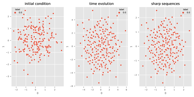
Figure 6.6: A heat equation solved with a Lagrangian method

This computation corresponds to a Brownian motion simulation, that is a stochastic process solving the stochastic ordinary differential equations $\frac{d}{dt}W_{t}=\mu$ with $\mu=\mathcal{N}(0,1)$ being the multi-dimensional normal law of unit variance and zero mean. These sequences can be computed for any stochastic processes having form $\frac{d}{dt}X_{t}=\nu(t,X_{t})dt+\sigma(t,X_{t})dW_{t}$, and we can check their strong convergence properties, as for the Heston model. (See [31].) The convergence rate of such variate is of order

$$\Big{|}\int_{\mathbb{R}^{D}}\varphi d\mu-\frac{1}{N}\sum_{i}\varphi(x^{i})\Big{|}\leq\frac{\mathcal{O}(1)}{N^{2}}$$

for any sufficiently regular function $\varphi$. This should be compared to a naive Monte-Carlo variate, converging at the statistical rate $\frac{\mathcal{O}(1)}{\sqrt{N}}$.

6.4.3 Convex-hull algorithm for Hamilton-Jacobi equations

Our next goal is to illustrate the Convex Hull Algorithm, see [30]. This method is concerned with nonlinear conservation laws, as the following Burgers-type equation having Dirichlet initial conditions:

$$\partial_{t}u+\nabla\cdot f(u)=0,\qquad u(0,\cdot)=u_{0},$$ (6.4.4)

where $f=(f_{d}(u))_{1\leq d\leq D}:\mathbb{R}\mapsto\mathbb{R}^{D}$ is a given flux and $\nabla\cdot f(u)=\sum_{1\leq d\leq D}\partial_{x_{d}}f_{d}(u)$ denotes its divergence, with $x=(x_{d})_{1\leq d\leq D}$. A Lagrangian method corresponds to determine a solution determined by the characteristic method. In the context of conservation laws, the characteristic method determines $u,y$ formally as (see (5.1.4) for a definition of the push-forward)

$$u(t,\cdot)=y(t,\cdot)_{\#}u_{0}(\cdot),\quad y(t,x)=x+tf^{\prime}(u_{0}(x)).$$ (6.4.5)

Provided $u_{0}$ is sufficiently regular, the transport function $y=y(t,x)$ defines an invertible map for small time $t$ and the equation (6.4.5) defines a unique solution to (6.4.4). However, we can show that $y(t,\cdot)$ is not one-to-one any longer for big enough times, for instance if $u_{0}$ is compactly supported. Nevertheless, $y(t,\cdot)_{\#}u_{0}(\cdot)$ still defines a formal solution to (6.4.4), calledthe energy conservative solution, that is highly oscillating, as can be seen in Figures 6.7-6.8 (middle), taking as flux $f(u)=(-u^{2},\cdots)$. The vanishing viscosity method allows one to select another, more physically relevant solution, called the entropy dissipative solution. It consists in solving in the limiting case $\epsilon\mapsto 0$ the following viscosity equation version of (6.4.5)

$$\partial_{t}u_{\epsilon}+\nabla\cdot f(u_{\epsilon})=\epsilon\Delta u_{\epsilon}.$$

For any $\epsilon>0$, the solution $u_{\epsilon}$ satisfies in a strong sense the entropy dissipation property $\partial_{t}U(u_{\epsilon})+\nabla\cdot F(u_{\epsilon})\leq 0$, for any convex entropy - entropy fluxes $U,F$. In the limiting case $\epsilon\mapsto 0$, this entropy dissipation holds in a weak sense. The CHA-algorithm allows an explicit computation of this vanishing viscosity solution, as

$$u(t,\cdot)=y^{+}(t,\cdot)_{\#}u_{0}(\cdot),\quad y(t,x)=x+tf^{\prime}(u_{0}(x)),$$

where $y^{+}(t,\cdot)$ is computed as

$$y^{+}(t,\cdot)=\nabla h^{+}(t,\cdot),\quad\nabla h(t,\cdot)=y(t,\cdot),$$

and $h^{+}(t,\cdot)$ is the convex hull of $h$. Figure 6.7 illustrates this computation for the onen-dimensional Burgers equation

$$\partial_{t}u+\frac{1}{2}\partial_{x}u^{2}=0,$$

since Figure 6.8 illustrates the two dimensional case $\partial_{t}u+\frac{1}{2}\nabla\cdot(u^{2},u^{2})=0$. The left-hand figure is the initial condition at time zero, since the solution at middle represent the conservative solution at time 1, and the entropy solution is plot at right.

Figure 6.7: Convex Hull algorithm

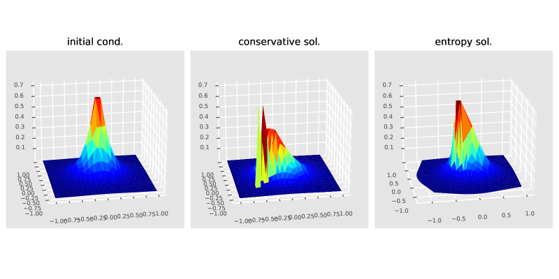
Figure 6.8: Convex Hull algorithm

6.5 Automatic differentiation

Adjoint Algorithmic Differentiation (AAD) is a family of techniques for algorithmically computing exact derivatives of compositions of differentiable functions. It is a useful tool for several applications in the present monograph; hence we describe it succinctly below.

Techniques for AAD have been known since at least the 1950s. There are two main variants of AAD: reverse-mode and forward-mode. Reverse-mode AAD computes the derivative of a composition of atomic differentiable functions by computing the sensitivity of an output with respect to the intermediate variables (without materializing the matrices for the intermediate derivatives). In this way, reverse-mode can efficiently compute the derivatives of scalar-valued functions. Forward-mode AAD computes the derivative by calculating the sensitivity of the intermediate variables with respect to an input variable. (Cf. [17].)

There are number of high quality implementations of AAD in the libraries, such as TensorFlow, PyTorch, autograd, Zygote, and JAX. The JAX supports both reverse-mode and forward-mode AAD.

CodPy also provides a simple interface to the Pytorch AAD differentiation framework. Figure 6.9 displays the computation of first- and second-order derivatives of a function $f(X)=\frac{1}{6}X^{3}$ using AAD.

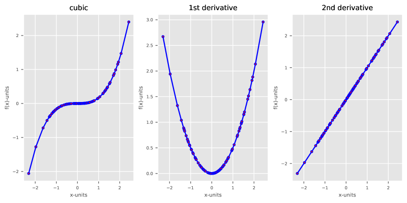
Figure 6.9: A cubic function, exact AAD first order and second order derivatives

6.5.1 Differential machine benchmarks

AAD is a natural tool to define a differential machine (2.1.4) starting from any predictive machine (2.1.1). Here, we illustrate a general multi-dimensional benchmark of two differential machines methods. The first one uses the kernel gradient operator (see (4.2.4) ). The second one uses a neural network defined with Pytorch together with AAD tools.

An example of one-dimensional testing is shown in Figure 6.10, using the same benchmark methodology as in chapter 2. The first row is quite similar to our one-dimensional test. The second row provides also four plots: the first one is the exact gradient of the considered function on the test set, computed using AAD. The second one plot the kernel gradient operator. The two remaining ones plot two different run of the neural network differential machine.

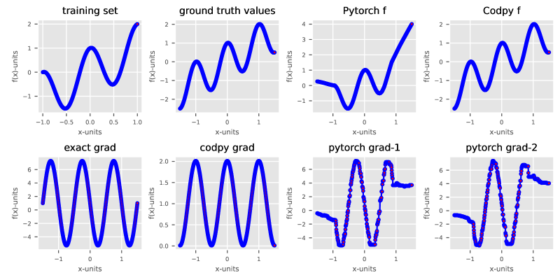
Figure 6.10: A benchmark of one-dimensional differential machines

The same benchmark can be used in any dimension, and we plot the two-dimensional test in Figure 6.11

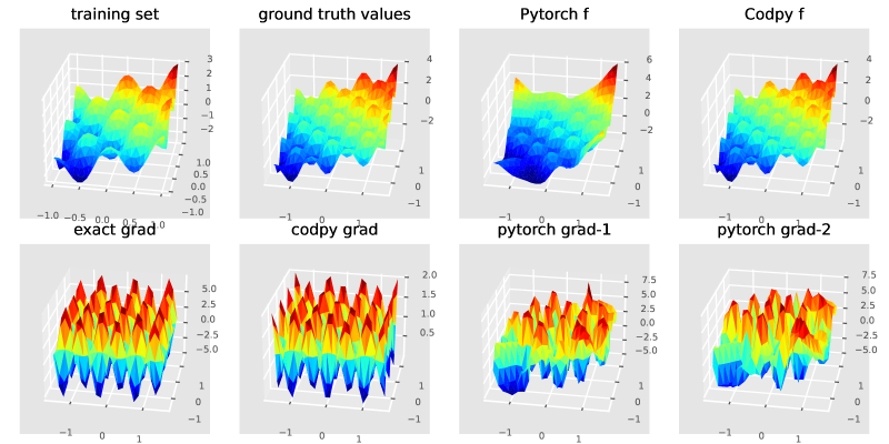
Figure 6.11: A benchmark of two-dimensional differential machines

Concerning these figures, we point out the following.

• Two runs of AAD computations leads to two different results (pytorch-grad1 and 2) : NNs do not define deterministic differential learning machines, due to the stochastic descent algorithm, here Adam optimizer.

• Differential neural networks tends to be less accurate than a kernel-based gradient operator.

6.5.2 Taylor expansions and differential learning machines

Taylor expansions using differential learning machines are common for several applications, hence we propose a general function to compute them, that we describe now. We start with the remainder of Taylor expansions.

Let us consider a sufficiently regular, vector-valued map $f$ defined over $\mathbb{R}^{D}$. Considering any sequences of points $Z,X$ having the same length, the following formula is called a Taylor’s expansion of order $p$:

$$f(Z)=f(X)+(Z-X)\cdot(\nabla f)(X)+\frac{1}{2}\Big{(}(Z-X)(Z-X)^{T}\Big{)}\cdot(\nabla^{2}f)(X)+\ldots+|Z-X|^{p}\epsilon(f),$$ (6.5.1)

where

• $(z-x)=\Big{(}z_{i}-x_{i}\Big{)}_{i,j=0..D}$ is a $D$-dimensional vector.

• $(z-x)(z-x)^{T}=\Big{(}(z_{i}-x_{i})(z_{j}-x_{j})\Big{)}_{i,j=0..D}$ is a $D,D$ matrix.

• $a\cdot b$ denotes the usual Frobenius inner product.

• $\nabla f$,$\nabla^{2}f$ holds for the gradient ($D$-dimensional vector) and the Hessian ($D,D$ matrix).

• $|z-x|$ is the standard Euclidean distance, $\epsilon(f)$ is a function depending on $f$ and its derivatives that we do not detail here. The term $|Z-X|^{3}\epsilon(f)$ represents the error committed by this approximation formula.

Let us now derive Taylor formulas using differential learning machines to approximate the derivatives, that is approximating $\nabla f(x)$,$\nabla^{2}f(x)$ with

$$\nabla f_{x}=\nabla_{Z}\mathcal{P}_{m}\big{(}X,Y,Z=x,f(X)\big{)},\nabla^{2}f_{x}=\nabla^{2}_{Z}\mathcal{P}_{m}\big{(}X,Y,Z=x,f(X)\big{)}.$$

Following the previous discussion, we performed a benchmark of a second-order Taylor formula using three approaches:

• The first one is the reference value for this test. It uses the AAD to compute both $\nabla f_{x},\nabla^{2}f_{x}$.

• The second one, uses a neural network defined with Pytorch together with AAD tools.

• The third one uses the hessian operator from CodPy.

The test is genuinely multi-dimensional, and we illustrate the one-dimensional case in Figure 6.12.

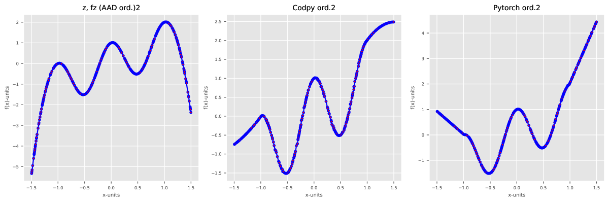
Figure 6.12: A benchmark of one-dimensional learning machine second-order Taylor expansion

6.6 Appendix: discrete high-order approximations

Let us denote the Taylor accuracy order $q>1$. Here, our purpose is to propose a general $q$-point formula in order to approximate any differential operator, accurate at order $q$. More precisely, consider a sufficiently regular function $f$, known at $q$ distinct points $f(x^{k})$, $x^{1}<\ldots,x^{q}$, and a differential operator $P^{\alpha}(\partial)=\sum_{i=0}^{q-1}p_{\alpha}^{i}(\partial^{i})$. For any function $f$, we want to approximate $(P^{\alpha}(\partial)f)(y)=\sum_{k=1}^{q}f(x^{k})$ at some points $y$. To this aim, consider the Taylor formula

$$f(x^{k})=f(y)+(x^{k}-y)\partial f(y)+\cdots=\sum_{i=0}^{q-1}\frac{(x^{k}-y)^{i}}{i!}(\partial^{i}f)(y),\quad k=1,\ldots,q$$

with the conventions $0!=1$, $\partial^{0}f=f$. Multiplying each line by $\beta_{y}^{k}$ and summing leads to

$$\sum_{k=1}^{q}\beta_{y}^{k}f(x^{k})=\sum_{i=0}^{q-1}(\partial^{i}f)(y)\sum_{k=1}^{q}\beta_{y}^{k}\frac{(x^{k}-y)^{i}}{i!}.$$

Hence, we rely on a $q-$point accurate formula for $P^{\alpha}(\partial)$, and we solve the following Van Der Monde-type system:

$$\sum_{k=1}^{q}\beta_{y}^{k}(x^{k}-y)^{i}=(i!)p_{\alpha}^{i},\quad i=0,\ldots,q-1.$$ (6.6.1)

Conversely, suppose a formula $(Pf)(y^{i})=\sum_{k=1}^{q}\beta^{k}_{y^{i}}f(x^{i-k})$ is given for distinct points $y^{1}<\ldots<y^{N_{y}}$. To recover $(Pf)f(x^{i})$, $i=q,\ldots,N_{x}$, we solve the following linear system:

$$(Pf)(x^{i})=\frac{(Pf)(y^{i})-\sum_{k=0}^{q-1}\beta^{k}_{y^{i}}f(x^{k})}{\beta^{k}_{y^{i}}},\quad i=q,\ldots,N_{x}.$$

Chapter 7 Application to supervised machine learning

7.1 Aims of this chapter

In this chapter and the following ones, we present some examples of concrete learning machines problems. Some of these tests are taken from kaggle.

Supervised learning problems can be split into regression problems and classification problems. Both of these have as a main goal the construction of a model that can predict the value of the output from certain input variables. In the case of regression, the output is a real-valued variable, whereas in the case of classification the output is a category such as a “disease” or “no disease” variable. Extrapolate and projection functions in CodPy are applied in order to deal with these problems.

Specifically, we are going to present two cases corresponding to each of these typical problems in supervised learning: Boston housing prices prediction and MNIST classification.

7.2 Regression problem: housing price prediction

Database. A database is provided which contains the information collected by the U.S Census Service concerning housing in the city of Boston (Massachusetts, USA). Here, there are 506 cases and 13 attributes (features) with a target column (price). We are interested in extrapolating these data. (Further details on this database can be found in [19] cited at the end of this monograph.)

Comparison between several methods. We rely on the extrapolation operator provided in CodPy and defined in (3.3.2) and compare tour results with several standard models of machine learning, namely: the decision tree (DT) in scikit-learn library and the neural network (NN) model in the TensorFlow library. Starting from the training set $X\in\mathbb{R}^{N_{x},D}$, we extrapolate the labels $f_{z}$, and compare to the labels of the test set denoted by $f(Z)$.

For the feed-forward NN we chose $50$ epochs with a batch size set of $16$, and we apply the Adam optimization algorithm with MSE as the loss function. The NN machine is composed of two hidden layers ($64$ cells), one input layer ($8$ cells), and one output layer with the following sequence of activation functions: RELU - RELU - RELU - Linear, respectively. All the remaining hyperparameters in the models are chosen to be equal to their default valued as provided in scikit-learn and TensorFlo, respectively.

Table 7.1: scenario list

$D$	$N_{x}$	$N_{y}$	$N_{z}$
-1	505	505	-1
-1	456	456	-1
-1	408	408	-1
-1	359	359	-1
-1	311	311	-1
-1	262	262	-1
-1	214	214	-1
-1	165	165	-1
-1	117	117	-1
-1	68	68	-1

The first plot in Figure 7.1 compares the methods in term of scores, while the second and third plots provide the discrepancy errors and execution time for different scenarii as defined in Table 7.1.

Interpretation of the results.

• First of all, observe that our RKHS-based method CodPy lab extra, namely the extrapolation method, leads us with, both, the best scores and the worst execution time.

• If we compare the discrepancy error to 1, the result matches the scores of the method CodPy lab extra. This indicates that the discrepancy error is an appropriate indicator.

• Another kernel method, CodPy lab proj,namely the projection method, is a more balanced method.

• Both kernel methods are performes here with a standard kernel, namely the Gaussian one, that is the only parameter for kernel methods. We emphasize that with kernel engineering we can easily improve these results. We do not present these improved kernel methods, as our purposes is to provide a benchmark with standard methods.

Observe that function norms and MMD errors are not method-dependent. Clearly, for this example, a periodical kernel-based method outperforms the two other ones. However, it is not our goal to illustrate an overall advantage of a particular method, but a benchmark methodology, particularly in the context of extrapolating test set data far from the training set data.

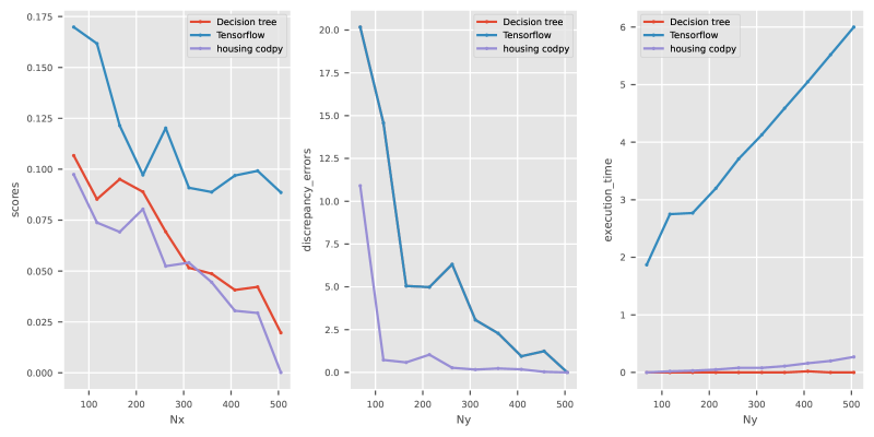
Figure 7.1: MMD and execution time

7.3 Classification problem: handwritten digits

MNIST Database. This section contains an example of a classification of images, which is a typical academic example referred to as the MNIST problem, and allows us to benchmark our results against more popular methods.

MNIST (“Modified National Institute of Standards and Technology”) contains 60,000 training images and 10,000 testing images. Half of the training set and half of the test set were taken from NIST’s training dataset, while the other half of the training set and the other half of the test set were taken from NIST’s testing dataset. Since its release in 1999, this classic database of handwritten images has served as the basis for benchmarking classification algorithms.

The MNIST dataset is composed of $60,000$ images defining a training set of handwritten digits. Each image is a vector with dimensions $784$, namely a $(28,28)$ grayscale image organized in row per row. There are $10$ possible digits, namely $0$ to $9$. The test set is composed of $10,000$ images with their labels.

We formalize the problem as follows. Given the test set represented by a matrix $X\in\mathbb{R}^{N_{x},D}$, $D=784$, the labels $f(X)\in\mathbb{R}^{N_{x},D_{f}}$, $D_{f}=10$, and the test set $Z\in\mathbb{R}^{N_{z},D}$, $N_{z}=10000$, predict the label function $f(Z)\in\mathbb{R}^{N_{z},D_{f}}$. Data are recovered from Y. LeCun MNIST home page this dedicated page for a description of the MNIST database, and we test here different values of the integer $N_{x}$.

For instance, the following plot shows an image of hand-written number, that is the first image $x^{1}$, as well as many other numbers:

Comparison between methods. We consider here different machine learning models in order to classify MNIST digits: support vector classifier (SVC), decision tree classifier (DT), adaboost classifier, random forest classifier(RF) by scikit-learn library and TensorFlow’s neural network (NN) model.

For the feed-forward NN we chose $10$ epochs with a batch size set of $16$, with Adam optimization algorithm and sparse categorial entropy as the loss function. The NN network is composed of $128$ input and $10$ output layers with a RELU activation function. All the remaining hyperparameters in the models are taken to be their default values given in scikit-learn or TensorFlow. On the other hand, we straightforwardly apply our projection operator (3.3.1) with the kernel defined by a composition of the Gaussian kernel with a mean distance map, where the training set is $X\in\mathbb{R}^{N_{x},784}$, and $Y\in\mathbb{R}^{N_{y},784}\subset X$ is randomly chosen.

Table 7.2: Scenario list

D	Nx	Ny	Nz
784	32	8	10000
784	64	16	10000
784	128	32	10000
784	256	64	10000

Scores are computed using the formula (2.3.1), a scalar in the interval $(0,1)$, which counts the number of correctly predicted images.

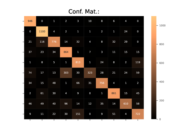
Figure 7.2: Confusion matrix for Neural network: Tensorflow

Figure 7.3 compares the methods in term of scores, MMD errors, andexecution time.

Interpretation of these results.

• First of all, observe that the kernel method CodPy class. extra is a multiple-input/multiple-output classifier, which is basically an extrapolation method. Itprovides us with, both, the best scores and the worst execution time.

• By computing 1 minus the discrepancy error, we match the scores of the method CodPy class. extra. This indicates that the discrepancy error is a relevant indicator here.

• Another RKHS-based method, namely CodPy class. proj, allows us to reduce the computational complexity of the extrapolation by using a projection of the input data to lower the dimensions. It is a more balanced method with respect to accuracy vs. complexity.

• Both kernel methods use a standard Gaussian kernel, that is the only parameter in the kernel methods. We emphasize that with kernel engineering we can easily improve these results. We do not present these improved kernel methods, as our purposes is to benchmark standard methods.

Observe that function norms and discrepancy errors are not method-dependent. Clearly, for this example, a periodic kernel-based method outperforms the two other ones. However, it is not our goal to illustrate a particular method supremacy, but a benchmark methodology, particularly in the context of extrapolating test set data far from the training set ones.

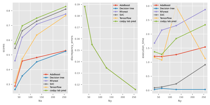
Figure 7.3: Scores, discrepancy errors and execution time for MNIST classification problem. The graph illustrates the performance indicators using different size of the training set.

7.4 Reconstruction problems : learning from sub-sampled signals in tomography.

Description. This numerical test allows us to now point out an interesting feature of learning machines to deal with reconstruction problems from sub-sampled signals. Indeed, in this test, we will be learning from a well-established algorithm, that is the SART one, to fasten the reconstruction.

There are many applications of such problems. We illustrate this section with a problem coming from a medical image reconstruction, that can be used also as a medical helping diagnosis decision tool. However, such problems occur in a wide variety of other situations: biology, oceanography, astrophysics, …

Poor input signal quality can sometimes be a choice. For instance, in nuclear medicine, it is better to work with lower radioisotopes concentration for obvious health reasons. Another interesting motivation for sub-sampling signals can be also accelerating data acquisition processes from expensive machines.

We illustrate this section with an example of such a reconstruction coming from reconstructing a signal from a sub-sampled SPEC (tomography) problem that we describe now.

Problem arising SPECT tomography. Our purpose now is to illustrate a sub-sampling reconstruction in the context of medical imagery, more precisely from sub-sampled SPECT images. To tist aim, we start from a set of high resolution images. The set itself is not really important for our objective in the present section. However it should be chosen carefully for an application to a real production problem.

This database image consists in a set of high resolution, $(512,512)$ images, consisting in approximately $30$ images of $82$ patients. The training set is built on the first $81$ patient. The 82-th patient is used for the test set. We first transform the training set database to produce our data. For each image in the training set (2470 images) we proceed as follows:

• We perform a “high” resolution $(256,256)$ radon transform , called a sinogram . A sinogram is quite similar to a Fourier transform of the original image, generating sinusoids.

• We perform a “low” resolution (8x256) radon transform.

• We reconstruct the original image from the high resolution sinogram to simulate high resolution SPECT images from these data. The reconstruction algorithm consists in computing an inverse radon transform .

An example of training set construction is presented Figure 7.4. Left is the reconstructed image from the “high resolution” sinogram (middle). The low resolution sinogram is plot at right.

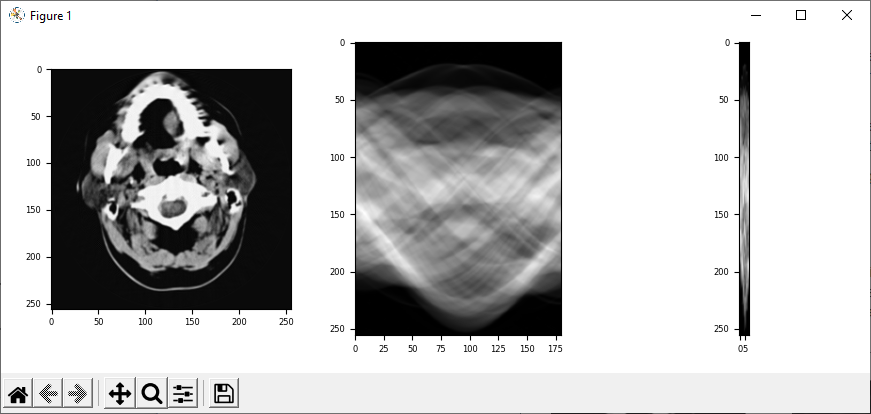
Figure 7.4: high resolution sinogram (middle), low resolution (right), reconstructed image (left)

The test consists then in reconstructing all images of the 82-th patient using low-resolution sinograms.

A comparison between methods. We present here the test resulting from a benchmark of a kernel-based method and the SART algorithm

Following our notations, section (2.1), we introduce

• The training set $x\in\mathbb{R}^{2473,2304}$, consisting in 2473 sinograms having resolution $8,256$, consisting in all low-resolution sinograms of the 81 first patients, plus the first one of the 82-th patient. This last figure is added to check an important feature in these problems : the learning machine must be able to retrieve an already input example.

• The test set $z\in\mathbb{R}^{29,2304}$, consisting in 29 sinograms of the 82-th patient, having resolution $8,256$.

• The training values set $f_{x}\in\mathbb{R}^{2473,65536}$, consisting in the 2473 images in “high-resolution”.

• The ground truth values $f(Z)\in\mathbb{R}^{29,65536}$, consists in 29 images in “high-resolution”.

• The first line, named exact, simply output the original figures, leading to zero error.

• The second one, named SART, reconstruct the figures from the SART algorithm with sub-sampled data.

• The third one, named CodPy, reconstruct the figures from the sub-sampled data with the kernel extrapolation method (3.3.2).

Figure 7.5 plots the first 8 images, presenting the original one at left, the reconstruction from SART algorithm, middle, and our algorithm, right. One can check visually that this kernel method better reconstruct the original image. It would be erroneous to conclude that this reconstruction process performs better than the SART algorithm, and it is not at all our speech here. We simply illustrate here the capacity of our algorithm to recognize existing patterns: indeed, note that the first image is perfectly reconstructed, as it is part of the training set. This property emphasizes that such methods suit well to pattern recognition problems, as automated tools to support professionals diagnosis.

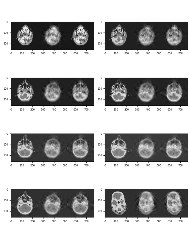
Figure 7.5: Example of reconstruction original (left), sub-sampled SART (middle), kernel extrapolation (right)

7.5 Appendix

Tables LABEL:tab:594 and LABEL:tab:601 indicates performance indicators for the Boston housing prices and MNIST datasets.

Table 7.3: Performance indicators for housing prices database

$predictors$	$D$	$N_{x}$	$N_{y}$	$N_{z}$	$D_{f}$	time	scores	discrepancies
housing codpy	13	505	505	506	1	0.27	0.0002	0.0000
housing codpy	13	456	456	506	1	0.20	0.0294	0.0376
housing codpy	13	408	408	506	1	0.16	0.0305	0.1803
housing codpy	13	359	359	506	1	0.11	0.0445	0.2339
housing codpy	13	311	311	506	1	0.08	0.0541	0.1693
housing codpy	13	262	262	506	1	0.08	0.0524	0.2742
housing codpy	13	214	214	506	1	0.05	0.0804	1.0383
housing codpy	13	165	165	506	1	0.03	0.0692	0.5876
housing codpy	13	117	117	506	1	0.02	0.0738	0.7295
housing codpy	13	68	68	506	1	0.00	0.0974	10.9051
Tensorflow	13	505	505	506	1	6.00	0.0886	0.0000
Tensorflow	13	456	456	506	1	5.52	0.0992	1.2415
Tensorflow	13	408	408	506	1	5.05	0.0969	0.9470
Tensorflow	13	359	359	506	1	4.59	0.0888	2.2870
Tensorflow	13	311	311	506	1	4.13	0.0909	3.0667
Tensorflow	13	262	262	506	1	3.71	0.1202	6.3171
Tensorflow	13	214	214	506	1	3.20	0.0972	4.9851
Tensorflow	13	165	165	506	1	2.77	0.1214	5.0520
Tensorflow	13	117	117	506	1	2.75	0.1617	14.5699
Tensorflow	13	68	68	506	1	1.87	0.1698	20.1727
Decision tree	13	505	505	506	1	0.00	0.0197	0.0000
Decision tree	13	456	456	506	1	0.00	0.0422	1.2415
Decision tree	13	408	408	506	1	0.02	0.0407	0.9470
Decision tree	13	359	359	506	1	0.00	0.0487	2.2870
Decision tree	13	311	311	506	1	0.00	0.0516	3.0667
Decision tree	13	262	262	506	1	0.00	0.0693	6.3171
Decision tree	13	214	214	506	1	0.00	0.0889	4.9851
Decision tree	13	165	165	506	1	0.00	0.0951	5.0520
Decision tree	13	117	117	506	1	0.00	0.0853	14.5699
Decision tree	13	68	68	506	1	0.00	0.1067	20.1727

Table 7.4: Performance indicators for MNIST database

$predictors$	$D$	$N_{x}$	$N_{y}$	$N_{z}$	$D_{f}$	time	scores	MMD
codpy lab pred	784	32	32	10000	1	1.37	0.5750	0.1882
codpy lab pred	784	64	64	10000	1	1.28	0.6974	0.1550
codpy lab pred	784	128	128	10000	1	1.84	0.7496	0.1346
codpy lab pred	784	256	256	10000	1	2.33	0.8286	0.1157
Tensorflow	784	32	32	10000	1	1.17	0.3115	0.1882
Tensorflow	784	64	64	10000	1	1.08	0.4732	0.1550
Tensorflow	784	128	128	10000	1	2.98	0.6345	0.1346
Tensorflow	784	256	256	10000	1	1.13	0.7668	0.1157
SVC	784	32	32	10000	1	0.09	0.5446	0.1882
SVC	784	64	64	10000	1	0.12	0.6634	0.1550
SVC	784	128	128	10000	1	0.23	0.7288	0.1346
SVC	784	256	256	10000	1	0.91	0.8105	0.1157
Decision tree	784	32	32	10000	1	0.03	0.2648	0.1882
Decision tree	784	64	64	10000	1	0.07	0.3569	0.1550
Decision tree	784	128	128	10000	1	0.03	0.4525	0.1346
Decision tree	784	256	256	10000	1	0.03	0.5243	0.1157
AdaBoost	784	32	32	10000	1	1.21	0.2878	0.1882
AdaBoost	784	64	64	10000	1	1.20	0.4581	0.1550
AdaBoost	784	128	128	10000	1	1.27	0.4819	0.1346
AdaBoost	784	256	256	10000	1	1.54	0.5289	0.1157
RForest	784	32	32	10000	1	1.68	0.4601	0.1882
RForest	784	64	64	10000	1	2.14	0.6199	0.1550
RForest	784	128	128	10000	1	2.30	0.7080	0.1346
RForest	784	256	256	10000	1	2.87	0.7771	0.1157

Chapter 8 Application to unsupervised machine learning

8.1 Aims of this chapter

We are going to apply some clustering methods for a number of use cases. We benchmarked our kernel-based algorithms (see Section 2.4.4 against the popular k-means algorithms. Both are distance-based minimization algorithms, aiming to solve the problem (4.3.1),which we recall here:

$$Y=\arg\inf_{Y\in\mathbb{R}^{N_{y},D}}d(X,Y).$$

The clusters $Y\in\mathbb{R}^{N_{y},D}$ are the results of this minimization algorithm:

• For k-means algorithm, the distance is called the inertia; see (2.3.5).

• For kernel-based algorithms, the distance is the kernel discrepancy or MMD; see (3.3.8).

Importantly, if the distance functional $d(X,Y)$ is not convex, then a solution to (4.3.1) might not be unique. For instance, a k-means algorithm usually produces different clusters at different execution runs.

8.2 Classification problem: handwritten digits

Database. The MNIST test is also studied in Section 7. Here we consider it as a semi-supervised learning: we use the train set $X\in\mathbb{R}^{N_{x},D}$ to compute the cluster’s centroids $Y\in\mathbb{R}^{N_{y},D}$. Then we use these clusters to predict the test labels $f_{z}\in\mathbb{R}^{N_{z},D_{f}}$, corresponding to the test set $Z\in\mathbb{R}^{N_{z},D}$.

Comparison between methods. First we use scikit’s k-means algorithm implementation, which is simply partitioning the input data $X\in\mathbb{R}^{N_{x},D}$ into $N_{y}$ sets so as to minimize the within-cluster sum of squares, which is defined as “inertia”. The inertia represents the sum of distances of all points to the centroid $Y\in\mathbb{R}^{N_{y},D}$ in a cluster. K-means algorithm starts with a group of randomly initialized centroids and then performs iterative calculations to optimize the position of centroids until the centroids stabilizes, or the defined number of iterations is reached.

Second we apply CodPy’s MMD minimization-based algorithm described in (4.3.1) using the distance $d_{k}(x,y)$ induced by a Gaussian kernel: $k(x,y)=\exp(-(x-y)^{2})$.

Table 8.1: scenario list

$D$	$N_{x}$	$N_{y}$	$N_{z}$
-1	1000	128	1000
-1	1000	256	1000

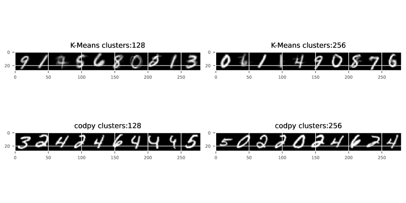
Figure 8.1: Scikit (the first row) and CodPy (second row) clusters interpreted as images

The result of k-means algorithm is $N_{y}$ clusters in $D=784$ dimensions, i.e. $Y\in\mathbb{R}^{N_{y},D}$. Note that the cluster centroids themselves are 784-dimensional points, and can themselves be interpreted as the “typical” digit within the cluster. Figure 8.1 plots some examples of computed clusters, interpreted as images. As can be seen, they are perfectly recognizable.

Finally, we show another benchmark plot, displaying the computed performance indicator of scikit’s k-means and CodPy’s MMD minimization-based algorithm in terms of MMD, inertia, accuracy scores (when applicable) and execution time, using scenarios in Table LABEL:tab:2999. The higher the scores and the lower are the inertia and MMD the better.

The scores are quite high, compared to supervised methods for similar size of training set, see results section (7). MMD-based minimization have an inertia indicator that is comparable to k-means. This is surprising as k-means algorithms are based on inertia minimization. Moreover, scores seems to indicate that the MMD distance is a more reliable criteria than inertia on this pattern recognition problem.

8.3 German credit risk

Database. The original dataset contains 1000 entries with 20 categorial/symbolic attributes. In this database, each entry represents a person who takes a credit by a bank. The goal is to categorize each person as good or bad credit risks according to the set of attributes.

Comparison between methods. The result of k-means and CodPy’s sharp discrepancy algorithm algorithm is $N_{y}$ clusters in $D$ dimensions. Notice that the cluster centroids themselves are $D$-dimensional points.

We visualize at figure 8.2 the clusters and corresponding centroids of scikit and CodPy’s sharp discrepancy algorithm, for 20 clusters.

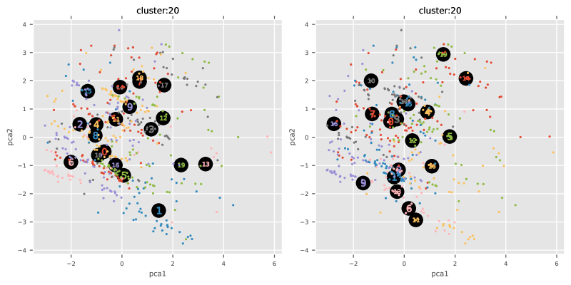
Figure 8.2: Scikit k-means (i) and codpy-MMD (ii)

Finally, we present a benchmark plot, displaying the computed performance indicators of scikit’s k-means and CodPy’s sharp discrepancy algorithms using scenarios from Table LABEL:tab:2999.

8.4 Credit card marketing strategy

Database. The problem can be formalized as follows. Develop a customer segmentation to define marketing strategy. The sample dataset summarizes the usage behavior of 8,950 active credit card holders during the last 6 months. The database contains 17 features and 8,950 records. The data describes customer’s purchase and payment habits, such as how often a customer installment purchases, or how often they make cash advances, how much payments are made, etc. By inspecting each customer, we can find which type of purchase he/she is keen on, or if the user prefers cash advance over purchases.

**Comparison between methods.*. The result of k-means algorithm and CodPy’s sharp discrepancy algorithm is $N_{y}$ clusters in $D$ dimensions. Note that the cluster centroids $Y\in\mathbb{R}^{N_{y},D}$ themselves are $D$-dimensional points.

Next we visualize the clusters and corresponding centroids of scikit’s k-means implementation CodPy’s sharp discrepancy algorithm, where we vary the number of clusters $N_{y}$ from $2$ to $4$.

Finally, we illustrate a benchmark plot, displaying the computed performance indicator of scikit’s k-means and CodPy’s sharp discrepancy algorithms.

8.5 Credit card fraud detection

Database. The database contains transactions made by credit cards in September 2013 by European cardholders. It presents transactions that occurred in two days, where we have $492$ frauds out of $284,807$ transactions. The database is highly unbalanced, the positive class (frauds) account for $0.172\%$ of all transactions.

The study addresses the fraud detection system to analyze the customer transactions in order to identify the patterns that lead to frauds. In order to facilitate this pattern recognition work, the k-means clustering algorithm is used which is an unsupervised learning algorithm and applied to find out the normal usage patterns of credit card users based on their past activity.

It contains only numerical input variables which are the result of a PCA transformation. The only features which have not been transformed with PCA are ‘Time’ and ‘Amount’. Feature ‘Time’ contains the seconds elapsed between each transaction and the first transaction in the database. The feature ‘Amount’ is the transaction Amount, this feature can be used for example-dependant cost-sensitive learning.

Feature ‘Class’ is the response variable and it takes value $1$ in case of fraud and $0$ otherwise.

Comparison between methods. Table 8.2 defines different scenarii of our test

Table 8.2: scenario list

$D$	$N_{x}$	$N_{y}$	$N_{z}$
-1	500	15	1000
-1	500	30	1000
-1	500	45	1000
-1	500	60	1000
-1	500	75	1000
-1	500	90	1000

Figure 8.3 illustrates confusion matrices for the last scenario of each approach.

Figure 8.3: confusion matrix for CodPy

Finally, we illustrate a benchmark plot, that shows the performance of scikit’s k-means and CodPy’s sharp discrepancy algorithms in terms of discrepancy errors, inertia, accuracy scores (when applicable) and execution time.

8.6 Portfolio of stock clustering

Database. This case represents daily stock price movements $X\in\mathbb{R}^{N_{x},D}$ (i.e. the dollar difference between the closing and opening prices for each trading day) from $2010$ to $2015$.

Table 8.3: Stock’s clustering

	k-means	MMD minimization
0	Apple, Amazon, Google/Alphabet	ConocoPhillips, Chevron, IBM, Johnson & Johnson, Pfizer, Schlumberger, Valero Energy, Exxon
1	Boeing, British American Tobacco, GlaxoSmithKline, Home Depot, Lookheed Martin, MasterCard, Northrop Grumman, Novartis, Royal Dutch Shell, SAP, Sanofi-Aventis, Total, Unilever	Intel, Microsoft, Symantec, Taiwan Semiconductor Manufacturing, Texas instruments, Xerox
2	Caterpillar, ConocoPhillips, Chevron, DuPont de Nemours, IBM, 3M, Schlumberger, Valero Energy, Exxon	Dell, HP
3	Intel, Navistar, Symantec, Taiwan Semiconductor Manufacturing, Texas instruments, Yahoo	Coca Cola, McDonalds, Pepsi, Philip Morris
4	Canon, Honda, Mitsubishi, Sony, Toyota, Xerox	Boeing, Lookheed Martin, Northrop Grumman, Walgreen
5	Colgate-Palmolive, Kimberly-Clark, Procter Gamble	AIG, American express, Bank of America, Ford, General Electrics, Goldman Sachs, JPMorgan Chase, Wells Fargo
6	Johnson & Johnson, Pfizer, Walgreen, Wal-Mart	British American Tobacco, GlaxoSmithKline, Novartis, Royal Dutch Shell, SAP, Sanofi-Aventis, Total, Unilever
7	Coca Cola, McDonalds, Pepsi, Philip Morris	Amazon, Canon, Cisco, Google/Alphabet, Home Depot, Honda, MasterCard, Mitsubishi, Sony, Toyota
8	Cisco, Dell, HP, Microsoft	Apple, Caterpillar, DuPont de Nemours, 3M, Navistar, Yahoo
9	AIG, American express, Bank of America, Ford, General Electrics, Goldman Sachs, JPMorgan Chase, Wells Fargo	Colgate-Palmolive, Kimberly-Clark, Procter Gamble, Wal-Mart

Comparison between methods. The table with a list of stocks shows that k-means clustering and MMD minimization displays stocks into coherent groups. Finally, we illustrate a benchmark plot, that shows the performance of scikit’s k-means and CodPy’s sharp discrepancy algorithms in terms of discrepancy errors, inertia, accuracy scores (when applicable) and execution time.

8.7 Appendix

Table 8.4: Performance indicators for MNIST dataset

$predictors$	$D$	$N_{x}$	$N_{y}$	$N_{z}$	$D_{f}$	time	scores	MMD	inertia
k-means	784	1000	128	10000	1	1.41	0.8017	0.3175	20073.11
k-means	784	1000	256	10000	1	2.56	0.8323	0.2087	14263.97
codpy	784	1000	128	10000	1	3.14	0.8690	0.1372	20210.97
codpy	784	1000	256	10000	1	5.20	0.8931	0.1318	14253.31

Table 8.5: Performance indicators for German credit database

$predictors$	$D$	$N_{x}$	$N_{y}$	$N_{z}$	$D_{f}$	time	MMD	inertia
k-means.	24	522	10	522	0	0.08	1.9052	7094.60
k-means.	24	522	20	522	0	0.14	1.0700	4756.91
codpy	24	522	10	522	0	0.03	0.9505	7175.53
codpy	24	522	20	522	0	0.03	0.5348	4756.91

Table 8.6: Performance indicators for credit card marketing database

$predictors$	$D$	$N_{x}$	$N_{y}$	$N_{z}$	$D_{f}$	time	discrepancies	inertia
k-means.	17	8950	2	8950	0	0.08	1.5309	127784.89
k-means.	17	8950	5	8950	0	0.11	4.6350	91776.61
k-means.	17	8950	8	8950	0	0.14	3.9432	74489.42
k-means.	17	8950	11	8950	0	0.19	3.3005	63635.62
k-means.	17	8950	14	8950	0	0.25	3.2431	57493.91
k-means.	17	8950	17	8950	0	0.27	2.6620	53270.74
k-means.	17	8950	20	8950	0	0.32	3.0762	49374.79
k-means.	17	8950	2	8950	0	0.07	1.5323	127785.07
k-means.	17	8950	5	8950	0	0.11	4.6350	91776.61
k-means.	17	8950	8	8950	0	0.12	3.9432	74489.42
k-means.	17	8950	11	8950	0	0.17	3.3005	63635.62
k-means.	17	8950	14	8950	0	0.27	3.2431	57493.91
k-means.	17	8950	17	8950	0	0.27	2.6620	53270.74
k-means.	17	8950	20	8950	0	0.30	3.0762	49374.79

Table 8.7: Performance indicators for credit card fraud database

$predictors$	$D$	$N_{x}$	$N_{y}$	$N_{z}$	$D_{f}$	time	scores	discrepancies	inertia
k-means	30	491	15	284316	1	0.33	0.9549	0.5198	20485.48
k-means	30	491	30	284316	1	0.39	0.9347	0.4550	13544.57
k-means	30	491	45	284316	1	0.36	0.9456	0.4291	10783.38
k-means	30	491	60	284316	1	0.52	0.9667	0.3990	8681.79
k-means	30	491	75	284316	1	0.48	0.9520	0.3674	7378.20
k-means	30	491	90	284316	1	0.55	0.9400	0.3805	6392.19
codpy	30	491	15	284316	1	17.96	0.9730	0.3364	20579.89
codpy	30	491	30	284316	1	18.53	0.9837	0.2571	13441.64
codpy	30	491	45	284316	1	18.55	0.9586	0.2301	10624.42
codpy	30	491	60	284316	1	19.65	0.9896	0.2178	8805.42
codpy	30	491	75	284316	1	18.75	0.9810	0.2063	7432.54
codpy	30	491	90	284316	1	20.06	0.9766	0.2023	6303.58

Table 8.8: Performance indicators for stock price

$predictors$	$D$	$N_{x}$	$N_{y}$	$N_{z}$	$D_{f}$	time	discrepancies	inertia
k-means.	963	60	10	60	0	0.09	0.7471	25.34
codpy	963	60	10	60	0	4.50	0.4568	25.41

Chapter 9 Application to generative models

9.1 Generating complex distributions

In this chapter, we consider encoder operators (5.1.1), decoder operators (5.1.2), and projection operators (5.1.3) in order to generate new images using the CelebA (Celebrities Attributes) dataset. CelebA is a large-scale dataset of over 200,000 celebrity faces with annotations for 40 attributes, including hair color, facial hair, glasses and hat. These images are normalized, having resolution 218x178 with 3 RGB colors, hence 116412 pixels. This database is widely used as input data for pattern recognition or training generative models.

In the context of image generation, the input is typically a set of real images and the expected output is a generated image that resembles the real images but with some variation. In the case of CelebA, the input is a set of celebrity images and the expected output is a generated image of a celebrity with specified attributes such as hair color or glasses. The goal of our test is to generate images that share close statistical properties from real images.

We used $N_{Y}=1000$ images of celebrity examples, denoted $Y=(y^{1},\ldots,y^{N_{Y}})$ in the training set. Thus the data’s dimension is $(1000,116412)$. We illustrate the encoding and decoding of this distribution see (5.1.1)-(5.1.2), with a latent variable space of size $D_{x}=4$.

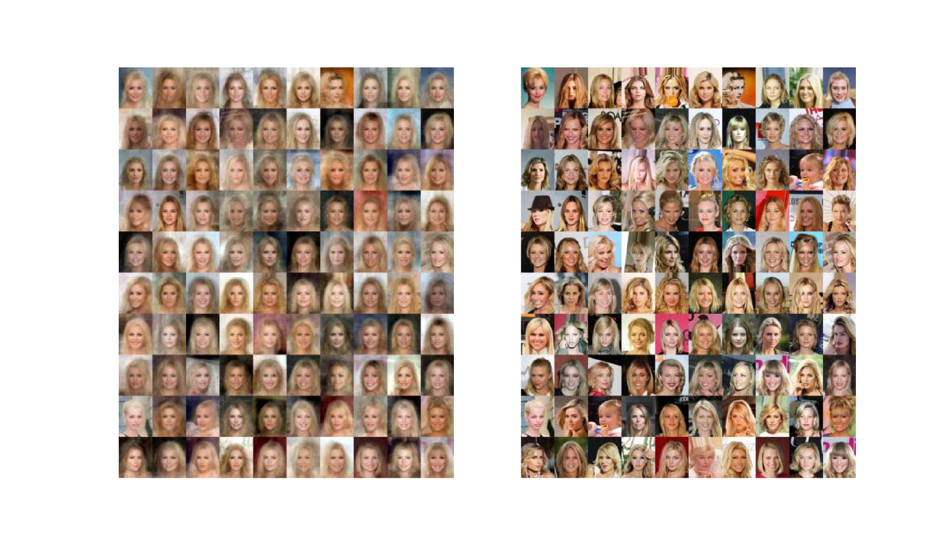
Figure 9.1: Original (right) and generated (left) images of CelebA dataset

In figure 9.1, the first plot displays $N_{z}=100$ generated images. They are obtained as decoding a latent variable being a variate of a white noise $Z=(z^{1},\cdots,z^{N_{z}})$in $D_{X}$ dimension. The plot at right shows the closest images, in the latent variables. To be precise, we used

$$y^{i(j)},\quad i(j)=\arg\inf_{j=1\ldots N_{x}}d_{k}(z^{i},l^{j}),$$ (9.1.1)

where $l^{j}\in\mathbb{R}^{D_{X}}$ is the latent variable attached to the picture $y^{j}$. Note that this matching algorithm in latent space leads to a quite efficient pattern recognition method.

Observe also that, as the dimension of the latent variable increases, the generated images tends to be more blurry. This is a dimensional effect : as the dimension increases, the distance between our training set latent variables and a random sample tends to increase also, and are statistically moving away from the training set. We somehow trade off variety for accuracy while tuning the dimension parameters $D$ of the latent space.

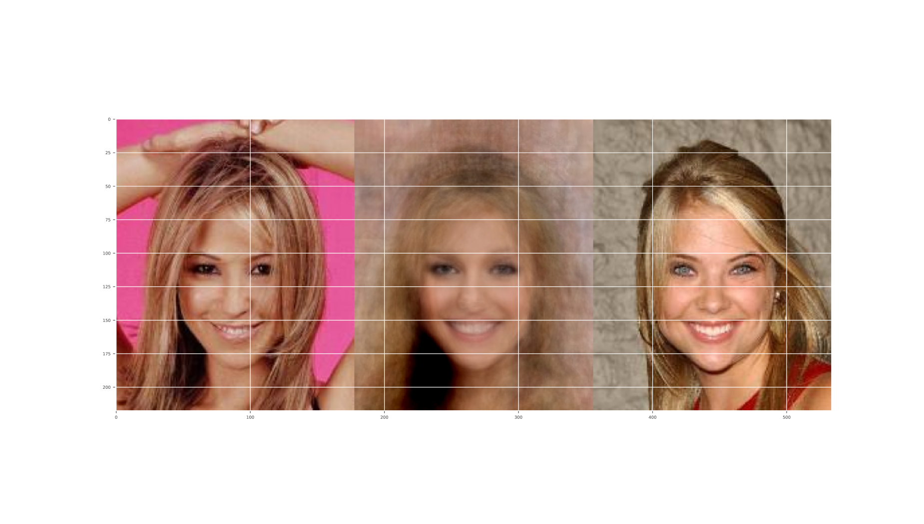
Figure 9.2: Original (left), reconstruction (middle) and closest pic (right) of the CelebA dataset

Figure 9.2 shows this effect with a 40 dimension latent space example, showing an example of reconstruction, see (5.1.3). Starting from the left-hand image, the middle image corresponds to its reconstruction, since the right-hand image is the closest image in the training set in the sense of (9.1.1). This militate towards pattern recognition algorithm using high=dimensional latent spaces, as both pictures are quite close in expression, and the reconstruction owns similarities with both pictures.

9.2 Estimation of conditional distributions

9.2.1 Data exploration

We start our journey to conditional distributions illustrating it with a small data exploration tool. To that aim, we consider the Iris dataset, introduced by Sir Ronald A. Fisher in 1936, which is a benchmark dataset in machine learning literature. It consists 150 samples from each of three species of Iris flowers (Iris setosa, Iris versicolor, and Iris virginica). Four features were measured from each sample: the lengths and the widths of the sepals and petals, and we consider conditioning on petal width. Hence, following the notations of Section 5.3.2, considering the Iris dataset $Z$, $X=Z[pet.width]$,$Y=Z[pet.leng,sep.leng,sep.wid]$.

In this experiment, given a specific petal width, we estimate the conditioned distribution and sample 500 examples for the others features.

We benchmark the three approaches of Section 5.3.2:

• The kernel generative conditioned method (5.3.3), with a latent space taken as a standard normal distribution in the three-dimensional space.

• Nadaraya-Watson algorithm (5.3.4), with a latent space taken taken as $Y$.

• The mixture distribution method (5.3.5).

The conditioning petal width is taken as the average petal width of the Iris dataset. We then resample upon conditioning and present the resulting cdf in Figure 9.3 against a reference distribution. Since there is no entry on the Iris dataset corresponding the average petal width $\overline{X}$,$\overline{\cdot}$ denoting the mean operator, we considered arbitrarily as reference distribution all those entries that are statistically close, more precisely selecting those entries $x$ satisfying $x-\overline{X}\leq\epsilon\text{ var}(X[\text{ petal width}])$. The threshold $\epsilon$ is chosen arbitrarily to 0.25, selecting a dozen of samples. The table 9.1 performs standard statistical test between generated distributions and this reference distribution.

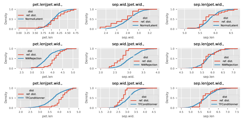
Figure 9.3:

Note that the previous picture plots the cdf of each sampled marginals, but do not give information on the full distributions. In Figure 9.4, we plot for one of our model a grid of figure, having the cdf at center, and representing the bi-marginal distributions for the outer diagonal items.

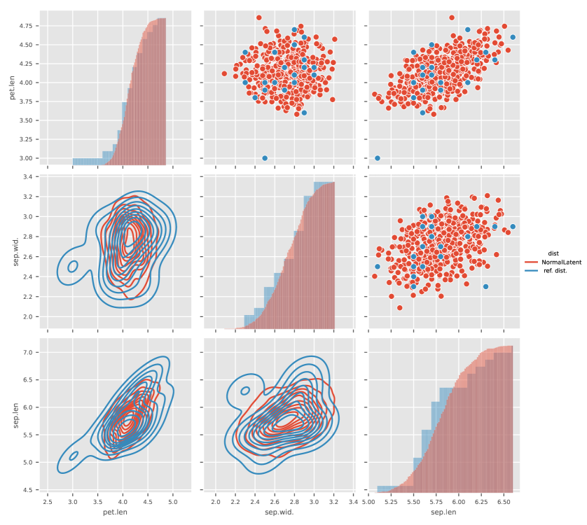
Figure 9.4:

Statistics on marginals can be found in Table 9.1. Note that statistical tests are hardly passed with this example, as the reference distribution is chosen arbitrarily and contains too few data. Nevertheless, with very few data, these algorithms can infer quite convincing conditional distributions.

Table 9.1: Stats

	Mean	Variance	Skewness	Kurtosis	KS test
NormalLatent:pet.len	4.1(4.1)	-1.2(0.12)	0.14(0.053)	3(-0.12)	0.3(0.05)
NormalLatent:sep.wid.	2.7(2.8)	-0.5(-0.13)	0.048(0.035)	-0.9(-0.28)	0.17(0.05)
NormalLatent:sep.len	5.8(5.8)	0.65(0.014)	0.13(0.073)	0.15(0.34)	0.041(0.05)
NWRejection:pet.len	4.1(3.8)	-1.2(0.38)	0.14(0.17)	3(0.72)	1.7e-06(0.05)
NWRejection:sep.wid.	2.7(3)	-0.5(-0.024)	0.048(0.12)	-0.9(-0.23)	6.8e-06(0.05)
NWRejection:sep.len	5.8(5.8)	0.65(0.2)	0.13(0.17)	0.15(0.68)	0.27(0.05)
TFConditionner:pet.len	4.1(3.7)	-1.2(-0.29)	0.14(0.27)	3(0.24)	6.6e-06(0.05)
TFConditionner:sep.wid.	2.7(3.1)	-0.5(-0.024)	0.048(0.19)	-0.9(0.37)	8.5e-07(0.05)
TFConditionner:sep.len	5.8(5.8)	0.65(0.19)	0.13(0.27)	0.15(0.055)	0.19(0.05)

9.2.2 Data completion

Next, we explore the possibilities of conditional generators to produce reliable synthetic datas. To that aim, we consider the Breast cancer wisconsin dataset, which is a benchmark dataset in machine learning literature. It consists 569 measurements of 30 patient’s numeric values, separated in two classes, malignant (212 entries) or benign (357). We consider the first four numeric values [mean radius, mean area, mean perimeter, mean texture]

Here, we separate the malignant class into two, having 106 elements each. The first half is used with the benign class as training set. The methodology is the following: we learn from a distribution having 463 entries, then resample 500 examples of the four features for the malignant class, and compare the generated distribution to the second malignant class. Figure 9.5 present, as in the iris case, the cdf at center, with the bi-marginal distributions for the outer diagonal items.

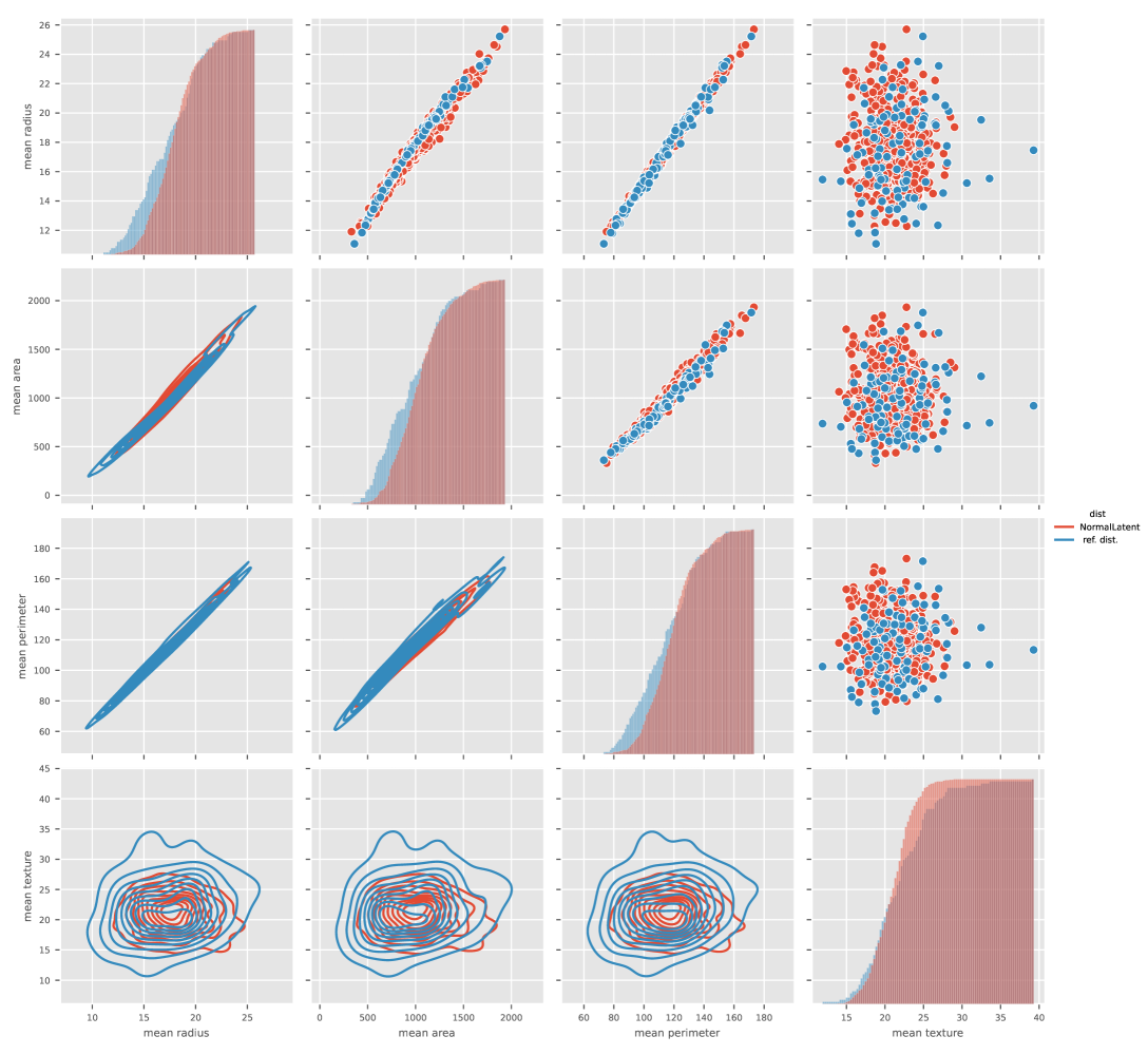
Figure 9.5:

The marginals statistics are available in Table 9.2. We noticed that the results are quite sensitive to the used kernel, and some kernel engineering might be necessary, mainly depending on distributions. For instance, a Cauchy kernel is quite well adapted to heavy tailed distributions. Here, we used a RELU type kernel to produce these results.

These tests should indicate that the sampled distribution is quite close to the reference one, although Kolmogorov-Smirnov tests are hardly passed.

Table 9.2: Stats

	Mean	Variance	Skewness	Kurtosis	KS test
NormalLatent:mean radius	17(18)	0.13(0.32)	9.1(5.3)	-0.56(0.1)	0.0042(0.05)
NormalLatent:mean area	9.6e+02(1e+03)	0.47(0.49)	1.1e+05(7.3e+04)	-0.24(0.14)	0.0028(0.05)
NormalLatent:mean perimeter	1.1e+02(1.2e+02)	0.2(0.34)	4.2e+02(2.6e+02)	-0.47(0.23)	0.011(0.05)
NormalLatent:mean texture	22(21)	0.92(0.034)	18(6.6)	2.3(-0.12)	0.0019(0.05)

9.2.3 Conditioning on discrete distributions

9.2.3.1 Circle example

Now we explore some aspects of conditioning on discrete, labeled values. In this first test, we consider a low-dimensional feature space $\mathcal{Y}$ consisting of 2D points $y=(y_{1},y_{2})$ lying on three circles chosen randomly, having corresponding label space $\mathbf{X}$ where $x$ can take one of three values $\{0,1,2\}$. These circles are displayed in Figure 9.6-(i).

Note that $\{1,2,3\}$ are labels in this problem, and should not be ordered. Hence we rely on hot encoding, to transform these labels into unordered ones, considering instead conditioning on a three-dimensional labels $\{1,0,0\},\{0,1,0\},\{0,0,1\}.$

Given a hot-encoded label $x_{i},i=1,2,3$, we generate samples two conditioning algorithms:

• The kernel generative conditioned method (5.3.3), with a latent space taken taken as $Y$, hence estimating the conditional probabilities $p(\mathbf{Y}|X=x_{i})$.

• Nadaraya-Watson algorithm (5.3.4), with a latent space taken taken as $Y$, hence sampling the conditional distributions $\mathbf{Y}|X=x_{i})$.

Doing so, we resample the original distribution, and we test the capability of the Nadaraya-Watson algorithm to properly identify the conditioned distribution, as well as this choice of latent variable for the kernel generative method.

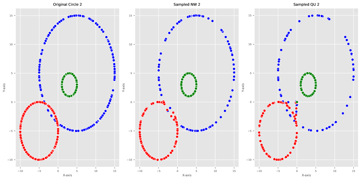
Figure 9.6:

As observed for simpler cases, the Nadaraya-Watson estimation and the generative conditioned method (5.3.3) infers close conditional probabilities, when they both use the same kernel and latent space, and the produced figures looks quite similars.

9.2.3.2 Latent variable role for complex conditioned distributions

As in Section 9.1, we highlight here too for conditional generators the role of the latent space dimension for a high dimensional feature space $\mathcal{Y}$, considering the MNIST examples. We picked up randomly $N=1000$ handwritten digits $Y\in\mathbb{R}^{1000,784}$, each picture being represented with $784$ pixels. These pictures are considered conditioned by ten labels $X\in\{0,\ldots,9\}^{1000}$, that are hot encoded.

A point worth mentioning is the difference of this approach with the supervised algorithm in section (7.3), where we learned the labels from the images to predict a label. Here we somehow learn the images from the labels, and we sample a new image from a label.

We study four algorithms:

• Nadaraya-Watson algorithm (5.3.4), with a latent space taken taken as $Y$.

• The kernel generative conditioned method (5.3.3), with a latent space taken taken as a standard normal distribution in dimension 784.

• The kernel generative conditioned method (5.3.3), with a latent space taken taken as a uniform distribution in dimension 2.

• The mixture distribution method (5.3.5).

For each label from $0$ to $9$, we use these algorithms to produce ten different samples, and the results are depicted figure 9.7.

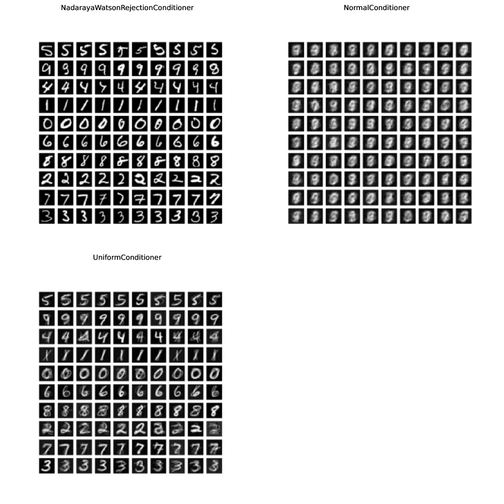
Figure 9.7:

Our conclusions are the following:

• As the latent space is $Y$ itself, the Nadaraya-Watson algorithm (5.3.4) do not produce new figures, but can identify quite confidently the proposed labels.

• The kernel generative conditioned method (5.3.3), as the mixture distribution method (5.3.5), produces averaged or noisy pictures. They both uses a high dimensional latent space.

• The kernel generative conditioned method (5.3.3), with a low dimensional latent space can produce credible new outputs.

9.2.3.3 Style transferts

In this test, we challenge conditional generators, changing some attributes of pictures of the celebA dataset. We consider a subsamples of 1000 images from this dataset, randomly selected among those pictures having the attributes [Woman, light make up]. We then consider those picture having the attributes [hat,glasses] (=[+,1,+1]) and select ten among them, depicted in the first row in Figure 9.8, to whom we would like to remove hat,glasses.

The 1000 images are handled by the generator (5.3.3), conditioned upon the two variables [hat,glasses], with a latent space consisting of a standard gaussian distribution having 25 dimensions. We keep constant all latent components of our 10 pictures, but the attributes [hat,glasses] that we we gradually switch from [+,1,+1], to [hat,glasses]=[-,1,-1] with constant steps of 0.4 for each row of Figure 9.8. The last row should be the resulting version of “no hat no glass” of our original pictures, and this test also check the continuity of the conditioned generator.

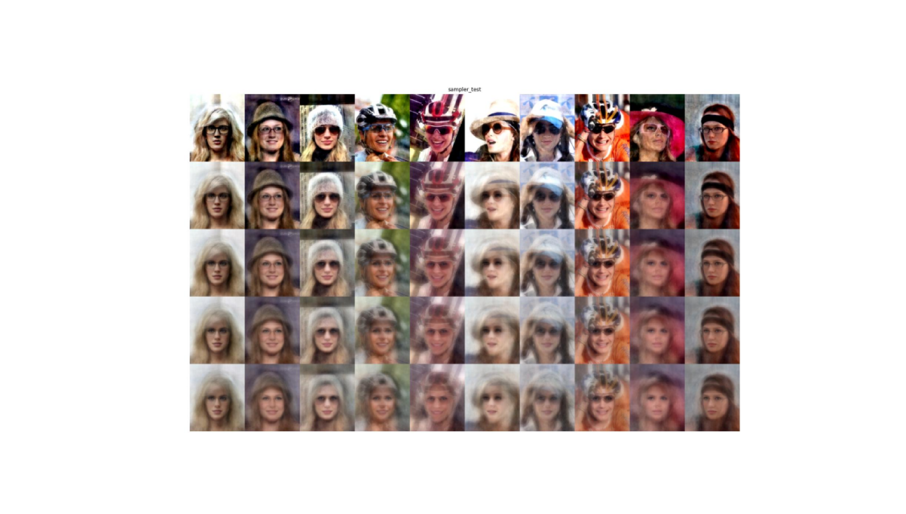
Figure 9.8: Removing hat and glasses from CelebA dataset pictures

For this exercise, the role of the latent space is quite important : if too big, the resulting pictures will look quite close to the original image, still wearing hat and glasses. If too small, there will be no longer any glass or hat, but the resulting pictures will look blurry and similar to each other. We tuned this parameter manually using trial and error to produce this figure. The result is mitigated: some of the resulting pictures are indeed without glass and hat, and we can see that these attributes faded in all pictures, but faces are hardly recognizable from the produced pictures in some cases. However, the purpose of this illustration is not to show state of the art image generation, but to illustrate what can be learnt from a small dataset. It illustrates also the difficulty to work with few examples, our main motivation to consider a small dataset is to keep the computation time within ten seconds CPU-time on a standard laptop from loading to image and output figures generation.

Chapter 10 Application to mathematical finance

We collect in this chapter a number of quite useful application of machine learning tools that are relevant for mathematical finance. The presentation is structured into two parts. The first part is dedicated to time series modeling and prediction, where we adopt an economic standpoint: starting from an historical data set consisting of one, or several, time series observations, we propose a framework capable to define a variety of stochastic processes matching these observations, that we can for forecasts. The second part focuses on pricing, which are computationally costly, time-dependent, functions defined on stochastic processes. Here, we show that classical supervised machine learning setting can be used to learn those functions. Once learned, we show that we can evaluate accurately those functions. This learning approach is a very numerical efficient one, and accurate enough to compute derivative of the pricing function. The resulting framework can then be used in a real-time setting, being a support to compute more sophisticated metrics, that can be used for risk management or investment strategies.

10.1 Free time series modeling

10.1.1 Setting and notations

We consider time series modeling as fitting a model in order to match a stochastic process $t\mapsto X(t)\in\mathbb{R}^{D}$, observed on a time grid $t^{1}<\ldots<t^{T_{X}}$, the data having the following shape

$$X=\Big{(}x^{n,k}_{d}\Big{)}_{d=1\ldots D}^{n=1\ldots N_{X},k=1,\ldots,T_{X}}\in\mathbb{R}^{N_{X},D_{X},T_{x}}.$$ (10.1.1)

In the following, we use a slicing notation such as $X_{\cdot}^{\cdot,k}=\Big{(}x^{n,k}_{d}\Big{)}_{d=1\ldots D}^{n=1\ldots N_{x}}\in\mathbb{R}^{N_{x},D_{X}}$. This describes a slice at the time $t^{k}$, since we use for the time index the third component of this 3-dimensional tensor. Whenever there is no confusion, we write in short $X^{k}$ for the time slices. In (10.1.1), $N_{x}$ is the number of observed samples of the time serie, thus $X^{n}=X^{n,\cdot}_{\cdot}$ is one trajectory. Observe that market data consist usually in observing only one trajectory of a stochastic process, hence $N_{x}=1$. However, in certain applications we might take $N_{x}\gg 1$, as for instance for customers data. Finally, the number of components of the observed process is $D$.

We illustrate the use of this notation with an example, downloading real market data recovered from January 1, 2020 to December 31, 2021, for three assets: Google, Apple and Amazon. These data are plot in Figure 10.1, and throughout this chapter serve to calibrate various models.

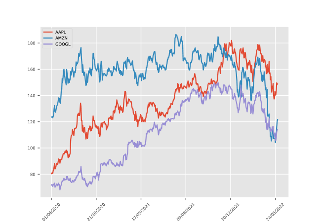
Figure 10.1: charts for Apple Amazon Google

For this figure and these data, we used the following global setting:

Table 10.1: Global settings

begin date	end date	pricing date	symbols
01/06/2020	01/06/2022	01/06/2022	AAPL , GOOGL, AMZN

10.1.2 Free time series models mappings

We call a free model, also called an agnostic model, the following framework for time series

$$F\Big{(}X\Big{)}=\varepsilon,$$ (10.1.2)

where:

• $\epsilon\in\mathbb{R}^{N_{\epsilon},D_{\epsilon},T_{\epsilon}}$, with possibly different sizes, that is $N_{\epsilon},D_{\epsilon},T_{\epsilon}$ can be different from $N_{X},D_{X},T_{X}$, is considered as a white noise, called latent, observed from the historical dataset applying the map $F$ to the time series, as $\epsilon=F\Big{(}X\Big{)}$.

• $F:\mathbb{R}^{N_{X},D_{X},T_{X}}\mapsto\mathbb{R}^{N_{\epsilon},D_{\epsilon},T_{\epsilon}}$ is a continuous map, that is supposed invertible, and we denote

  $$X=F^{-1}\Big{(}\varepsilon\Big{)}.$$ (10.1.3)

Observe that this framework allows one to combine simpler maps together. For instance, suppose that we consider two different models, involving two maps $F_{1},F_{2}$, with $\text{Im }(F_{2})\subset\text{Supp }(F_{1})$, then $F:=F_{1}\circ F_{2}$ provides another model, with $F^{-1}=F_{2}^{-1}\circ F_{1}^{-1}$.

In particular, consider any given invertible map $F$, a given time serie $X$, and observe a noise $\epsilon=F(X)$. Then one always can compose it with the encoder mapping, see (5.1.1), transforming this noise into another one, $\tilde{\epsilon}=\mathcal{L}(\epsilon)$. Or, if we believe that an exogeneous distribution $\mathbb{Y}$ is causal for the noise $\epsilon$, one can use a conditioning map (5.3.2) to retrieve $\tilde{\epsilon}=\mathcal{L}(\epsilon,\mathbb{Y})$,

The strategy followed in this section consists in the following:

• First observe $\epsilon$ from data, applying $\eqref{MF}$ to the historical observations $X$. Consider that $\epsilon_{\cdot}^{n,k}$ are $N_{x}\times T_{X}$ variates of a white noise $\epsilon$.

• Generate new samples of the latent variable $\tilde{\epsilon}$.

• Use the inverse formula, computing $\tilde{X}=F^{-1}(\tilde{\epsilon})$. This amounts to sample new trajectories, according to a given model (10.1.2).

The purpose of this approach is to allow for various applications as follows:

• Benchmarking strategies. Picking up $t^{*k}=t^{k}$, this corresponds to re-sample the original signal $X$ on the same time-lattice. This allows to draw several simulated trajectory and to compare it to the original one using various performance indicators.

• Monte-Carlo forecast simulations. The idea is quite similar to the previous applications, but for future times $t^{*}=[t^{N_{X}}<t^{*0}<\ldots]$.

• Forward Calibration. This case corresponds to a perturbation of the previous case, expressed as a minimization problem with constraints having form $\inf_{Y}d(X,Y)$, const. $\mathbb{E}(P(X^{\cdot,*k}))=c_{p}$, where $d$ is a distance, $P$ a vector-valued function and $c_{p}$ a real-valued vector.

• PDE pricers, that are multidimensional trees, capable to compute forward prices or sensitivities by solving backward Kolmogorov equations.

We claim that the framework (10.1.2) is quite a universal one, into which fit most of the known quantitative models for time series analysis. Such models are usually built on top of known processes, as Brownian motions. We can reconsidered them as built upon an unknown random variable $\epsilon$, that is observed with historical data and reproduced by generative methods. We can then reinterpret these models as random walk processes. This allows to better model short term dynamic of stochastic processes. Moreover, machine learning proposes new calibration methods. Finally, this framework allows to define new quantitative models, as will be illustrated later on this section.

10.1.3 Random walks and Brownian motion mappings

To motivate the framework (10.1.2), consider a random walk process

$$X^{k+1}=X^{k}+\epsilon^{k}.$$ (10.1.4)

A random walk process fit the framework (10.1.2) with a difference map

$$\epsilon=\delta_{0}(X):=X^{k+1}-X^{k}$$

The inverse of this map (10.1.3) is the integration map

$$X=\sum\epsilon:=X^{0}+\sum_{l=0}^{k-1}\epsilon^{l},\quad k=0,\ldots$$

In particular, provided $\epsilon^{k}$ are retrieved as variates of a centered random variable $\epsilon$, the central limit theorem states that $\frac{X^{k}}{\sqrt{k}}\mapsto\mathcal{N}(0,\sigma)$, a normal law having zero-mean and variance matrix $\sigma=\text{var }(\epsilon)\in\mathbb{R}^{D_{X},D_{X}}$, as $k\mapsto\infty$, in a distributional sense.

Observe also that a Brownian motion $W_{t}$ fits also the framework (10.1.2) with $F$ defined as

$$\delta_{\sqrt{t}}(W_{t})=\Big{(}\delta_{\sqrt{t}}^{k}(W_{t})\Big{)}_{k=0,\ldots},\quad\delta_{\sqrt{t}}^{k}(W_{t}):=\frac{W_{t^{k+1}}-W_{t^{k}}}{\sqrt{t^{k+1}-t^{k}}},$$

$ since the inverse map is given by

$$\sum_{(1/2)}\epsilon:=\Big{(}W_{t^{0}}+\sum_{l=0}^{k-1}\Big{(}\sqrt{t^{l+1}-t^{l}}\Big{)}\epsilon^{l}\Big{)}_{k\geq 0}.$$

The last expression coincides with the Euler-Maruyama scheme for simulating a Brownian motion, that is $W_{t^{k+1}}=W_{t^{k}}+\mathcal{N}(0,\sigma\sqrt{t^{k+1}-t^{k}})$, with $\sigma=\text{Var }(\epsilon)$.

Let us now illustrate the strategy pointed in the introduction with the Log-normal process. Log-normal maps can fit any positive time series, and are popular to model simple stock markets dynamic. These maps are simply the composition of the Log map:

$$\epsilon=(\delta_{0}\circ\text{Log })(X)=\Big{(}\ln(X^{k+1})-\ln(X^{k})\Big{)}_{k=0,\ldots}.$$ (10.1.5)

Defining the log-normal map. Its inverse mapping is

$$X=(\delta_{0}\circ\text{Log })^{-1}(\epsilon)=\Big{(}\text{Exp }\circ\sum_{0}\Big{)}^{-1}(\epsilon):=\Big{(}X^{0}\exp(\sum_{l=0}^{k-1}\epsilon^{l})\Big{)}_{k=1,\ldots}.$$ (10.1.6)

Consider also the classical Euler scheme for Log-Normal dynamics

$$X_{t}=X_{s}\exp(\sqrt{t-s}\epsilon).$$ (10.1.7)

Then this scheme can also be summarized as

$$X=(\delta_{\sqrt{t}}\circ\text{Log })^{-1}(\epsilon)=\Big{(}\text{Exp }\circ\sum_{(1/2)}\Big{)}^{-1}(\epsilon):=\Big{(}X^{0}\exp(\sum_{l=0}^{k-1}\sqrt{t^{k+1}-t^{k}}\epsilon^{l})\Big{)}_{k=1,\ldots}.$$

The Euler scheme (10.1.7) provides the explicit form of (10.1.2) as an integral-type operator, summarized with the expression $X=X^{0}\Big{(}\text{Exp}\circ\sum_{(1/2)}\Big{)}(\epsilon)$.

From the historical data set 10.1, we compute the log-return random variable $\epsilon$ appearing at (10.1.7), illustrated in the left part of the figure 10.2 on its two first components (AMAZ,APPL). We can use the encoder setting (5.1.1) to map this noise to any, latent, known distribution, as for instance a uniform distribution. We then generate another variate of the latent distribution, and use the inverse map, the decoder (5.1.2), to simulate a variate of the observe noise $\epsilon$, plot at right of figure 10.2.

Figure 10.2: Log return distribution of historical and generated data

It is crucial to test whether the generated distribution is statistically close to the original, historical one. The table 10.2 compute various statistical indicators, as the fourth moments and Kolmogorov-Smirnov tests, to challenge the generative method

Table 10.2: Stats for historical (generated) data

	0	1	2
Mean	0.0012(0.00054)	-3e-05(0.00032)	0.00091(0.00067)
Variance	-0.066(-0.09)	-0.44(0.029)	-0.09(-0.19)
Skewness	0.0004(0.00034)	0.0005(0.00041)	0.00033(0.00026)
Kurtosis	2(0.57)	6.7(2)	1.4(0.62)
KS test	0.48(0.05)	0.93(0.05)	0.31(0.05)

We then resample our model using

$$X=X^{0}\Big{(}\text{Exp}\circ\sum_{1/2}\circ\mathcal{L}^{-1}\Big{)}(\eta),$$

where $\eta$ is a white noise generated with the known random variable. Ten examples of resampling are plot figure 10.3.

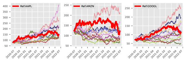
Figure 10.3: Ten examples of generated paths with the free Euler scheme

10.1.4 Auto-regressive, moving averages maps

Auto-regressive, moving averages ARMA(p,q) are popular, causal models for univariates time series. They can be expressed as follows

$$X^{k}=\mu+\sum_{i=1}^{p}a_{i}X^{k-i}+\sum_{i=1}^{q}b_{i}\mathbb{X}^{k-i},$$ (10.1.8)

where $\mathbb{X}^{k-i}$ are white noise, that are random variables satisfying $\mathbb{E}(\mathbb{X}^{i})=0$, $\mathbb{E}((\mathbb{X}^{i})^{2})=\sigma^{2}$, $Cov(\mathbb{X}^{i},\mathbb{X}^{j})=0,i\neq j$, and $\mu$ is the mean of the process. ARMA processes proposes several methods to calibrate the coefficients $a_{i},b_{i},\sigma$, as linear regressions, nonlinear least squares, or maximum likelihood methods. Thus we suppose in the sequel that the coefficients $a_{1},\ldots,a_{p}$, $b_{1},\ldots,b_{q}$ are given.

In the context of free-models, we do not suppose any longer that $\mathbb{X}^{k}$ are white noise random variables, and we can straightforwardly generalize to the multidimensional case.

The expression (10.1.8) gives straightforwardly the map (10.1.2). To compute the inverse map (10.1.3), we use the following relations, see [8]

$$\mathbb{X}^{k}=\mu+\sum_{j=0}^{\infty}\pi_{j}X^{k-j},$$

where the coefficients $\pi_{j}$ are determined by the relations

$$\pi_{j}+\sum_{k=1}^{\min(p,q)}b_{j}\pi_{j-k}=-a_{j}:=\pi_{j}+\phi(B)(\pi_{j}),\quad j=0,1,\ldots,$$

with the convention $a_{0}=-1$, $a_{i}=0$, for $i>p$, and $b_{j}=0$, for $j>q$. We introduced the backshift operator $B(\pi^{k})=\pi^{k-1}$ and $\phi(B)(\pi^{j})=\sum_{k=1}^{\min(p,q)}b_{j}\pi_{j-k}$. Considering range of values where this operator is invertible, we can denote its inverse $\phi^{-1}(B).$

For the numerics, we consider the autoregressive model of order $p$, denoted $AR(p)$ which is $ARMA(p,1)$ model. The mapping (10.1.2) is here $\phi(B)(X^{k})=\epsilon^{k}$, and its inverse $X^{k}=\phi^{-1}(B)(\epsilon^{k})$. The figure 10.4 shows example of ten generated trajectories with this AR(p) model.

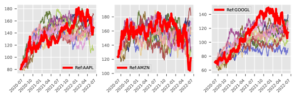
Figure 10.4: Ten examples of generated paths with the ARMA(p,1) Model

10.1.5 GARCH(p,q) maps.

The generalized autoregressive conditional heteroskedasticity (GARCH) model of order $(p,q)$, commonly used in the field of financial time series analysis, characterizes a stochastic process $X_{t}$ with a variance that depends on its past values. The $GARCH(p,q)$ model is defined as follows:

$$\left\{\begin{array}[]{cc}X^{k}=\mu+\sigma^{k}Z^{k},\\ (\sigma^{k})^{2}=\alpha_{0}+\sum_{i=1}^{p}\alpha_{i}(X^{k-i})^{2}+\sum_{i=1}^{q}\beta_{i}(\sigma^{k-i})^{2}.\end{array}\right.$$

Here, $\mu$ is the mean, $\sigma^{k}$ is a stochastic variance process, and $Z^{k}$ is a white noise process. The parameters $\alpha_{i}$ and $\beta_{i}$ denote the GARCH parameters.

We can express the variance process $(\sigma^{k})^{2}$ in terms of the backshift operator $B$:

$$(1-\beta(B))(\sigma^{k})^{2}=\alpha_{0}+\alpha(B)(X^{k})^{2},$$

Where $\alpha(B)=\sum_{i=1}^{p}\alpha_{i}B^{i}$ and $\beta(B)=\sum_{i=1}^{p}\alpha_{i}B^{i}$. Set $\varphi(B)=\alpha_{0}+\sum_{i=1}^{p}\alpha_{i}B^{i}$, $\theta(B)=1-\sum_{i=1}^{q}\beta_{i}B^{i}$ and $\pi(B)=\varphi^{-1}(B)\theta(B)$ to get $\sigma_{t}$ as

$$\sigma^{k}=\sqrt{\varphi^{-1}(B)\theta(B)(X^{k})^{2}}=\sqrt{\pi(B)(X^{k})^{2}}.$$

From here, assuming that we can obtain the white noise process:

$$Z^{k}=G(X^{k})=\sqrt{\varphi(B)\theta^{-1}(B)(X^{k})^{2}}(X^{k}-\mu)=\sqrt{\pi^{-1}(B)(X^{k})^{2}}(X^{k}-\mu).$$

The transformation $G:X^{k}\mapsto Z^{k}$ can be referred to as the ‘GARCH map’.

Figure 10.5 shows example of ten generated trajectories using GARCH(1,1) model.

Figure 10.5: Ten examples of generated paths with the GARCH(1,1) Model

10.1.6 Lagrange interpolation mapping

Next, we consider a map that is quite similar to the AR(p) one, that is

$$L^{(2p)}(X)=(X^{-p+k},\ldots,X^{+p+k})=\sum_{i=-p}^{p}\beta^{i}_{t^{k*}}X^{k-i},\quad k=p,\ldots,T_{X}-p,$$ (10.1.9)

where $t^{*k}=\frac{t^{k}+t^{k+1}}{2}$, and the coefficients $\beta^{i}_{t^{k*}}$ are retrieved as a $p$ Lagrange interpolation in time, that is solving the following VanDerMonde-type system (6.6.1), that is

$$\sum_{l=-p}^{p}\beta^{i}_{t^{k*}}(t^{k-p}-t^{*k})^{i}=\delta(i,0),\quad i=0,\ldots,2p,$$ (10.1.10)

where $\delta(i,j)=\{i=j:1,\ \text{else: }0\}$. This interpolation corresponds to a model of a time series that is not only determined by causal effects (the positive index $i$ appearing at (10.1.9)), but that also include market anticipation effects (the negative indices $i$ appearing in (10.1.9)).

Figure 10.6 shows an example of resampling of our historical dataset using this Lagrange interpolation with $p=10$ and the map $F^{-1}:=X_{0}\text{ Exp }\circ L^{-(10)}\circ\sum_{0}\circ\mathcal{L}^{-1}(\eta)$.

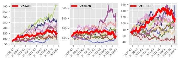
Figure 10.6: Ten examples of generated paths with Lagrange interpolation

10.1.7 Additive noise map

We now consider a map $\eta_{\mathbb{Y}}(\epsilon)$ that consists in conditioning $\epsilon$ by $\mathbb{Y}$. This conditioning is specified as an additive noise model

$$\eta_{Y}(\epsilon)=\epsilon-G(Y),\quad\eta_{Y}^{-1}(\epsilon)=\epsilon+G(Y),$$ (10.1.11)

where

• $\eta_{Y}$ is a white noise, that is an independent random variable.

• $G(Y)\in\mathbb{R}^{D_{\epsilon}}$ is a smooth function. If $G$ is unknown, the denoising procedure (6.3.1) proposes a way to calibrate it using historical observation.

For instance, we can elaborate on the ^∗ model (10.1.9), defining as map $F:=\eta_{Y}\circ\delta_{0}\circ L^{2p}\circ\text{ Log}$, where $Y=X^{*}\circ\text{ Log}(X)$. The whole model can then be summarized as follows:

$$\ln X^{*,k+1}=\ln X^{*,k}+G\Big{(}\ln X^{*,k}\Big{)}+\epsilon^{k}.$$

This particular conditioning map was thought primarily to capture models following a stochastic differential equations as Vasicek model, having form $\delta r_{t}=F(r_{t})\delta_{t}+dW_{\delta_{t}}$.

Applying this model produce the resampling of our historical dataset plot at figure 10.7. Note that $G$ is calibrated to historical data, using the algorithm (6.3.1), with $\epsilon=10^{-3}$, $X=\{X^{*,k}\}_{k=0,...}$ and $F=\{\epsilon^{*,k}\}_{k=0,...}$.

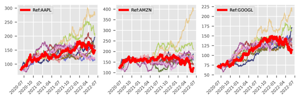
Figure 10.7: Ten examples of generated paths with additive map

10.1.8 Conditioned map and data augmentation

Next, we consider conditioning maps. As a first example, any noise $\epsilon$ can be conditioned by the process itself, that is we can consider $(\epsilon,X)$ as a joint variable and estimate the distribution

$$\mathcal{L}(\epsilon)=\epsilon|\mathbb{X}.$$ (10.1.12)

, Numerically, we approximate this conditioned distribution by the map (5.3.2). The map composition $\mathcal{L}\circ\Delta\circ Log$ defines the following scheme

$$\ln X^{k+1}=\ln X^{k}+\Big{(}\varepsilon^{k}\ |\ \ln X^{k}\Big{)}.$$ (10.1.13)

This scheme produced the resampling of our historical dataset plot in Figure 10.8

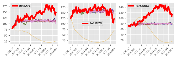
Figure 10.8: Ten examples of generated paths with the conditionning model

The scheme (10.1.13) is expected to capture (weakly) stationary stochastic processes, as CIR (Cox, Ingelson Rox) processes. Observe that (10.3.8) allows also for data augmentation, that is adding extra information to the original dataset. For instance, consider the following map

$$\sigma(X)=\Big{(}\sigma^{k}(X)\Big{)}_{0\leq k},\quad\sigma^{k}(X):=\text{Tr (covar) }\Big{(}X^{k-q},\cdots,X^{k+q}\Big{)},$$

where $q$ is an integer provides, and Tr(covar) holds for the trace of the covariance matrix. Any distribution $\epsilon$ can then be conditioned to this variance. In particular, consider the following scheme:

$$\begin{split}\ln X^{k+1}&=\ln X^{k}+\varepsilon_{X}\ |\ \sigma^{k}\\ \sigma^{k+1}&=\sigma^{k}+\varepsilon_{\sigma}|\ \sigma^{k},\end{split}$$ (10.1.14)

where $\varepsilon=(\varepsilon_{X},\varepsilon_{\sigma_{q}})$ are the noise components defined, produced the figure 10.9

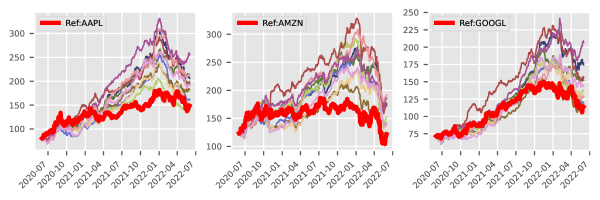
Figure 10.9: Ten examples of generated paths with the stochastic volatility model

The model (10.1.14) is expected to capture stochastic volatility type processes (ass Heston, GARCH, …).

10.2 Benchmark Methodology

Next, we propose a general method to evaluate the generative stochastic models presented in the previous section, and apply it to two of the presented model for illustration purposes. In a nutshell, the method proposes to study synthetic paths generated by observing a single path of a known stochastic processes, and we consider here the Heston model, as this model is built upon an unseen variable, modeling a stochastic volatility process. Our motivation here is to benefit from known results, as closed formula for evaluation purposes, to check and benchmark our models. Accordance with closed formula is the last test, the tests being carried out in several stages, the aim being to better understand these models, and to provide a methodology to design and tune them.

The methodology proceeds as follows:

$\bullet$ Setting: We choose a known stochastic process model (here the Heston one) under study and select the associated parameters. Then we generate a path, that will be used as the historical dataset.

$\bullet$ Calibration : Starting from this path, we pick a free time series model and calibrate it to the historical dataset. We also calibrate the parameters of the stochastic process to match this trajectory (the Heston model is defined through a set of eight parameters).

$\bullet$ Reproduction : We ensure that the generated model can reproduce the initial process. This step is crucial for the generative framework $\eqref{MF}$, in order to check that the map is invertible.

$\bullet$ Distribution : Also specific to our generative framework, we check that the distribution of the noise $\epsilon$ (see (10.1.2)) computed from the historical data and the generative model are consistent, using graphical and statistical tests.

$\bullet$ Trajectories : We regenerate trajectories with these new parameters using the same library as for the initial trajectory, and compare this with the method derived from the generative model.

$\bullet$ Pricing : We consider a function, given by the payoff of an option, and evaluate its expectation by performing a naive Monte Carlo method both the known process, as well as the generative one, comparing them to a closed formula whenever possible.

In the following sections we apply this methodology to three different methods considering a Heston process. The first is a calibrated Heston process, and the two others are different generative models from our framework, namely the log diff one (10.1.5).

10.2.1 Benchmarks framework - Heston

We recall that the Heston model is described by the following SDE

$$dX_{t}=\mu X_{t}dt+X_{t}\sqrt{\nu_{t}}dW_{t}^{1},$$

where

$$d\nu_{t}=\kappa(\theta-\nu_{t})dt+\sigma\sqrt{\nu_{t}}dW_{t}^{2},\quad<dW_{t}^{1},dW_{t}^{2}>=\rho$$

With a given set of Heston parameters $\mu,\kappa,\theta,\rho,X_{0},\nu_{0}$, satisfying the Feller condition $2\kappa\theta>\sigma^{2}$, we generate one path, that is represented in bold red in the figures 10.12. Observing this path, we calibrate $\mu=\frac{\ln(X_{T})}{\ln(X_{0})}$ and regenerate several paths, pictured in Figure 10.12-i). These paths will serve us later on to benchmarks our models.

10.2.2 Reproducibility

First of all, we check that the generated model can reproduce the initial process since the map can be reverted.

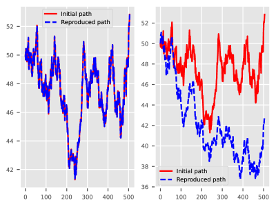
Figure 10.10: Reproducibility test for a Heston process

10.2.3 Benchmarks distributions

We then use these same trajectories to compare the log normal distributions of the two methods, which are then matched with a statistical table.

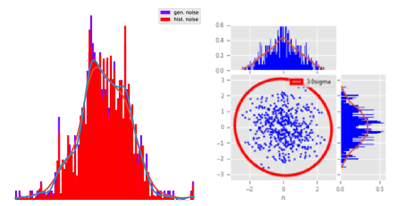
Figure 10.11: Calibrated Model compared to Generative

Table 10.3: Statistical table – Generative Stats(Calibrated ones)

	Mean	Variance	Skewness	Kurtosis	KS test
HestonDiffLog lat.:0	0.00011(0.00013)	-0.045(-0.044)	9.8e-05(9.8e-05)	0.8(0.72)	1(0.05)
HestonCondMap lat.:0	-0.0024(0.018)	0.00053(0.18)	0.9(0.68)	-0.42(0.056)	0.0088(0.05)
HestonCondMap lat.:1	-0.0032(-0.025)	0.0073(0.15)	1(0.97)	-0.49(-0.046)	0.0063(0.05)

10.2.4 Benchmarks trajectories

Here we compare $1000$ trajectories generated on the left by a Heston SDE with approximated parameters, and on the right what the generative model has reproduced from the initial input trajectory. In both graphs, the initial trajectory we wish to reproduce is shown in red color.

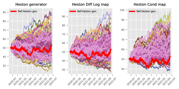
Figure 10.12: Model generated paths compared to synthetic Heston ones

10.2.5 Benchmarks prices

With the initial SDE we create a vanilla option, in this case a European Call with strike K given by the last value of the initial sample and maturity t=T, i.e. the end of the process. We calculate the price by performing a Monte Carlo on the trajectories of the two methods, and compare it with the closed formula.

Table 10.4: Heston Calls price

	MC :PricesDiffLog	Gen :PricesDiffLog	closed pricer	Gen :PricesCondMap
Mean	7.141976	8.552551	7.222894	7.988374
Var	79.254114	101.864179	NaN	58.212532
Lower bound	6.590205	7.927006	NaN	7.515488
Upper bound	7.693747	9.178096	NaN	8.461260

10.3 Pricing with generative methods

Let $t\mapsto X_{t}$ a Markov process, $V(T,\cdot)$ a function representing a payoff having maturity $T$. For pricing, the quantities of interest are the following:

$$\overline{V}(s,T,y)=\mathbb{E}^{\mathbb{Q}}_{X_{s}=y}\Big{(}V(T,X_{T})\Big{)},$$ (10.3.1)

where $\mathbb{Q}$ is the standard notation of the neutral risk measure. We distinguish between the function $V$ and its expectation, using the overline notation $\overline{V}$.

Observe that the previous sections allow to consider Monte-Carlo methods to estimate (10.3.1). However, for a number of applications, one needs to compute not only one single value, that is the price, —which is $\overline{V}(0,T,X_{0})$ in the above setting— but also all of the fair value surface $(s,y)\mapsto\overline{V}(s,T,y)$ (for $0\leq s\leq T$ and $y\in\text{Im}(X_{s})$). This latter observation is important in an operational context, since all standard risk measures can be determined from the knowledge of this surface, such as measures of internal or regulatory nature, or optimal investment strategies.

In such a context, Monte-Carlo methods are intractable, so we propose an alternative strategy in this section.

10.3.1 Transition probabilities of agnostic models

Consider a given model (10.1.2) calibrated to a time serie $X$. We note the $t^{0}<\ldots<t^{T_{X}}$ the time grid of the historical dataset, as well as $t^{*,0}<\ldots<t^{*,T_{X}}$ the predicted time grid; see also (10.1.1) for the notation. Our aim now is to estimate the transition probabilities of a model satisfying the model (10.1.2), that is:

$$\Pi^{l,k}:=\Big{(}\pi_{n,m}^{l,k}\Big{)}_{n,m=0}^{N_{X}^{*}},\quad\pi_{n,m}^{l,k}:=\mathbb{E}\Big{(}X^{*n,k}|X^{*m,l}\Big{)},\quad l=1,\ldots,\ l<k$$ (10.3.2)

A way to estimate this conditional distribution is to generate numerous trajectories and to use the conditioning map (5.3.2). However, this approach is computationally intensive, and we propose an alternative approach in this section.

10.3.2 A reminder on Fokker-Plank and Kolmogorov equations

Let us recall the definition of a stochastic differential equation (SDE) describing the dynamics of a Markov-type stochastic process, denoted by $t\mapsto X_{t}\in{\mathbb{R}}^{D}$, i.e.

$$dX_{t}=G(X_{t})dt+\sigma(X_{t})dW_{t}.$$ (10.3.3)

Here, $W_{t}\in\mathbb{R}^{D}$ denotes a $D$-dimensional, independent Brownian motion, while $G\in\mathbb{R}^{D}$ is a prescribed vector field and $\sigma\in\mathbb{R}^{D\times D}$ is a prescribed matrix-valued field.

Denote by $\mu=\mu(t,s,x,y)$ (defined for $t\geq s$) the density probability measure associated with $X_{t}$, knowing the value $X_{s}=y$ at the time $s$. We recall that $\mu$ obeys the Fokker-Planck equation, which is the following nonlinear partial differential equation (defined for $t\geq s$):

$$\partial_{t}\mu-\mathcal{L}\mu=0,\quad\mu(s,\cdot)=\delta_{y},$$ (10.3.4)

which is a convection-diffusion equation. Moreover, the initial data is the Dirac mass $\delta_{y}$ at some point $y$, while the partial differential operator is

$$\mathcal{L}\mu:=\nabla\cdot(G\mu)+\nabla^{2}\cdot(A\mu),\quad A:=\frac{1}{2}\sigma\sigma^{T}.$$ (10.3.5)

Here, $\nabla$ denotes the gradient operator, $\nabla\cdot$ the divergence operator, and $\nabla^{2}:=(\partial_{i}\partial_{i})_{1\leq i,j\leq D}$ is the Hessian operator. We are writing here $A\cdot B$ for the scalar product associated with the Frobenius norm of matrices. We emphasize that weak solutions to (10.3.4) defined in the sense of distributions must be considered, since the initial data is a Dirac mass.

The (vector-valued) dual of the Fokker-Planck equation is the Kolmogorov equation, also known in mathematical finance as the Black and Scholes equations. This equation determine the unknown vector-valued function $\overline{P}=\overline{P}(t,x)$ as a solution to, with $t\leq s$,

$$\partial_{t}\overline{P}-\mathcal{L}^{*}\overline{P}=0,\quad\mathcal{L}^{*}\overline{P}:=-G\cdot\nabla\overline{P}+A\cdot\nabla^{2}\overline{P}.$$ (10.3.6)

By the Feynmann-Kac theorem, a solution to the Kolmogorov equation (10.3.6) can be interpreted as a time-average of an expectation function. Hence our strategy is to solve Kolmogorov equations (10.3.6) instead of a Monte-Carlo method. It also allows to take into account sophisticated strategies based on derivatives, or american exercizing.

10.3.3 Covariance conditioned map

Now, we consider a map $B$ that consists in modeling the noise $\epsilon$ using a matrix-valued distribution $B$, determined by the following Poisson equation

$$\nabla\cdot B(\epsilon)=\epsilon,\quad\epsilon\in\mathbb{R}^{D_{\epsilon}},B(\epsilon)\in\mathbb{R}^{D_{\epsilon},D_{\epsilon}},$$ (10.3.7)

$\nabla\cdot$ denoting the divergence operator. The mapping $\epsilon\mapsto B(\epsilon)$ somehow smooth out the noise $\epsilon$, at the expense of increasing its dimensionality. The resulting matrix field is then conditioned to an external variable, for instance $X$, as described in the previous section. We summarize this in the following

$$B(\epsilon)^{k}=\mathbb{E}\Big{(}\big{(}\nabla\cdot\big{)}^{-1}(\epsilon^{k})|X^{k}\Big{)}\in\mathbb{R}^{D_{X},D_{X}},$$ (10.3.8)

where the conditioner $\mathbb{E}$ is approximated by (5.3.2).

For instance, we can further reduce the noise in (10.1.13) by considering the map $B_{Y}\circ\gamma_{Y}\circ\eta_{Y}\circ\delta_{0}\circ L^{(2p)}\circ\text{ Log}(X)$. This generated Figure 10.13 for $N=100$ trajectories. Note that this simulation is becoming quite accurate, as we checked that the historical dataset lies above our sampled trajectory set for $\sim$ 5 occurrences on each underlying. This is in accordance with the fact that we resampled 100 trajectories over 500 time plots.

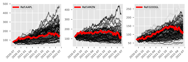
Figure 10.13: Hundred examples of generated paths with conditioned covariance map

10.3.4 A toy risk management system

Next, we describe an alternative approach to non-parametric models, producing synthetic data using kernel methods. Indeed, the capability to reproduce a given random variable accurately is key to synthetic data. This is illustrated with a toy example of risk management in this section:

• We consider an econometry, that are historical time series of market data, as well as a portfolio of financial instruments, that are functions depending on these market data.

• We then use a generative method to forecast the time series.

• We use a predictive method to forecast our financial instrument values.

10.3.4.1 Settings a portfolio of instruments

We define a payoff function as $P(t,x)\mapsto P(t,x)\in\mathbb{R}^{D_{P}}$, with $D_{P}$ corresponding to the number of instrument. We consider here a single instrument $D_{P}=1$, the instrument being a basket option written on our underlyings, that is

$$P(t,x)=\max(<\mathcal{X}\cdot x>-K,0.)$$

where $<\mathcal{X}\cdot x>$ are the basket values, $\mathcal{X}$ being the weights, and $K$ is called the option’s strike. We represent this payoff in a two-dimensional figure with axis basket values in left=hand plot in Figure 10.14.

We attached a pricing function as a payoff, that is a vector-valued function $(t,x)\mapsto P(t,x)\in\mathbb{R}^{D_{P}}$. We represent this pricing function in a two-dimensional right figure 10.14 with axis basket values.

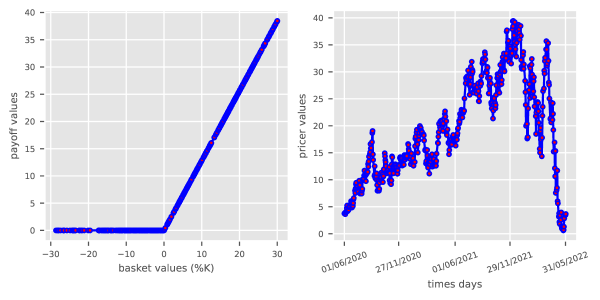
Figure 10.14: Pricing as a function of time

The pricing function here is selected as a simple Black and Scholes formula, hence hypothesizing that the basket values are log normal

10.3.4.2 Predictive methods for financial applications

We now use the projection operator $P_{k}$ (see (3.3.1)) in order to predict the pricing function plot in Figure 10.14 on unseen, intraday market values $z$. We first discuss our choice of training set $X,f(X)$. According to (3.3.7), the interpolation error committed by the projection operator $P_{k}$, defined on a training set $X$, is driven at any point $z$ by the quantity $D_{k}(z,X)$. We plot at figure 10.15 the isocontours of this error function for two distinct training sets (blue dots). In these figures, the test set is plot in red. and corresponds to simulated, intraday, market values, that are produced synthetically for this experiment using the sampler function.

• (right) $X$ is generated as VaR scenarios for three dates $t^{0}-1,t^{0},t^{0}+1$, with $H=10$ days horizon. VaR (Value at Risk) means here producing synthetical datas at time $t^{0}+H$, corresponding to what is referenced as *historical* VaR.

• (left) $X$ is the historical data set.

The test set is generated as VaR scenarios with 5 days horizon (blue dots).

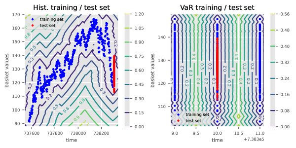
Figure 10.15: Training and test set

This figure motivates the choice of VaR-type scenario dataset as training set, right-hand plot in Figure 10.15, in order to minimize the interpolation error. Note that using the historical data set, might be of interest, if only historical data are available.

Observe finally that there are three sets of red points at Figure 10.15-(a), as we considered VaR scenarios at three different times $t^{0}-1,t^{0},t^{0}+1$, because we are interested in approximating time derivatives for risk management, as the theta $\partial_{t}P$.

We plot the results of two methods to extrapolate the pricer function on the test set $Z$ (CodPy = kernel prediction, taylor = Taylor second order approximation) in Figure 10.16.We also plot the reference price (exact = reference price). We compared to a Taylor formula, widely used in an operational context.

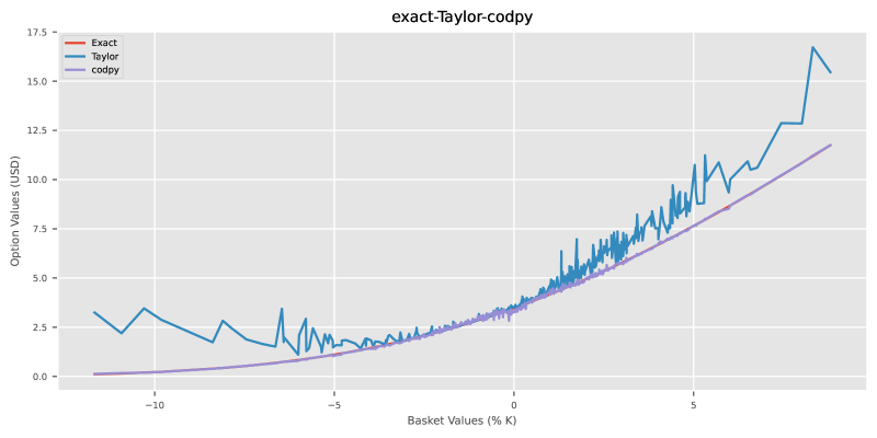
Figure 10.16: Prices output

We can also compute greeks, using the operator $(\nabla_{k}P)_{Z}$ defined at (4.2.4). Here too, we plot the results of two methods to extrapolate the gradient of the pricer function on the test set $Z$ (CodPy = kernel prediction, taylor = Taylor second order approximation) in Figure 10.17. We also plot the reference greeks (exact = reference greeks). This figure should thus produce $(\nabla_{k}P)_{Z}=\big{(}(\partial_{t}P)_{Z},(\partial_{x_{0}}P)_{Z},\ldots,(\partial_{x_{D}}P)_{Z}\big{)}$, that are $D+1$ plots.

Note that raw deltas computed with this method present spurious oscillations, because our training set is obtained as a iid variate, thus we used the denoising procedure (6.3.1), to smooth them out.

Figure 10.17: Greeks output after correction

Bibliography

- [1] A. Antonov and M. Konikov and M. Spector, The free boundary SABR: natural extension to negative rates, unpublished report, January 2015, available at https://ssrn.com/abstract=2557046.
- [2] I. Babuska, U. Banerjee, and J.E. Osborn, Survey of mesh-less and generalized finite element methods: a unified approach, Acta Numer. 12 (2003), 1–125.
- [3] A. Berlinet and C. Thomas-Agnan, Reproducing kernel Hilbert spaces in probability and statistics, Springer US, Kluwer Academic Publishers, 2004.
- [4] M.A. Bessa, and J.T. Foster, T. Belytschko, and W.K. Liu, A mesh-free unification: reproducing kernel peridynamics, Comput. Mech. 53 (2014), 1251–1264.
- [5] A. Brace, and D. Gatarek and M. Musiela, The market model of interest rate dynamics, Math. Finance 7 (1997), 127–154.
- [6] H. Brezis, Remarques sur le problème de Monge–Kantorovich dans le cas discret, Comptes Rendus Math. 356 (2018), 207–213.
- [7] Y. Brenier, Polar factorization and monotone rearrangement of vector-valued functions, Comm. Pure Applied Math. 44 (1991), 375–417.
- [8] P.J. Brockwell, and R.A. Davis Time series: theory and methods, Springer Series in Statistics, 2006.
- [9] H. Buehler, Volatility and dividends: volatility modeling with cash dividends and simple credit risk, February 2010, available at: https://ssrn.com/abstract=1141877.
- [10] F. Eckerli and J. Osterrieder, Generative adversarial networks in finance: an overview, Comput. Methods Appl. Mech. Engrg.(2021).
- [11] G.E. Fasshauer, Mesh-free methods, in “Handbook of Theoretical and Computational Nanotechnology”, Vol. 2, 2006.
- [12] G.E. Fasshauer, Mesh-free approximation methods with Matlab, Interdisciplinary Math. Sciences, Vol. 6, World Scientific Publishing Co. Pte. Ltd., Hackensack, NJ, 2007.
- [13] G.E. Fasshauer, Positive definite kernels: past, present and future, unpublished report, available at http://www.math.iit.edu/ fass/PDKernels.pdf.
- [14] A. Gretton, K.M. Borgwardt, M. Rasch, B. Schölkopf, and A.J. Smola, A kernel method for the two sample problems, Proc. 19th Int. Conf. on Neural Information Processing Systems, 2006, pp. 513–520.
- [15] B.Schölkopf, R. Herbrich, and A.J. Smola, A generalized representer theorem. In Computational learning theory, Springer Verlag, 2001, pp. 416–426.
- [16] F.C. Günther and W.K. Liu, Implementation of boundary conditions for meshless methods, Comput. Methods Appl. Mech. Engrg. 163 (1998), 205–230.
- [17] A. Griewank and A. Walther, Evaluating derivatives: principles and techniques of algorithmic differentiation, SIAM Publication, 2008.
- [18] E. Haghighat, M. Raissib, A. Moure, H. Gomez, and R. Juanes, A physics-informed deep learning framework for inversion and surrogate modeling in solid mechanics, Comput. Methods Appl. Mech. Engrg. 379 (2021), 113741.
- [19] D. Harrison and D.L. Rubinfeld, Hedonic prices and the demand for clean air, J. Environ. Economics & Management 5 (1978), 81–102.
- [20] T. Hastie, R. Tibshirani, and J. Friedman, Elements of statistical learning: data mining, inference, and prediction, Springer Series in Statistics, 2009.
- [21] T. Hofmann, B. Schölkopf, and A.J. Smola, Kernel methods in machine learning, Ann. Statist. 36 (2008), 1171–1220.
- [22] B.N. Huge and A. Savine, Differential machine learning, unpublished report, January 2020, available at https://ssrn.com/abstract=3591734
- [23] T.F. Korzeniowski and K. Weinberg, A multi-level method for data-driven finite element computations, Comput. Methods Appl. Mech. Engrg. 379 (2021), 113740.
- [24] J.J. Koester and J.-S. Chen, Conforming window functions for mesh-free methods, Comm. Numer. Methods Engrg. 347 (2019), 588–621.
-
[25]
Y. LeCun, C. Cortes, and C.J.C. Burges,
The MNIST database of handwritten digits,
http://yann.lecun.com/exdb/mnist/ - [26] R. McCann, Polar factorization of maps on Riemannian manifolds, Geom. Funct. Anal. 11 (2001), 589–608.
- [27] P.G. LeFloch and J.-M. Mercier, Fully discrete, entropy conservative schemes of arbitrary order, SIAM J. on Numer. Anal. 40 (2002), 1968–1992.
- [28] J.-M. Mercier, Optimally transported schemes with applications to mathematicalfFinance, unpublished report, available at https://www.researchgate.net/publication/228689632_Optimally_Transported_schemes_Applications_to_Mathematical_Finance
- [29] J.-M. Mercier, A high-dimensional pricing framework for financial instruments valuation, DOI:10.2139/ssrn.2432019.
- [30] P.G. LeFloch and J.-M. Mercier, Revisiting the method of characteristics via a convex hull algorithm, J. Comput. Phys. 298 (2015), 95–112.
- [31] P.G. LeFloch and J.-M. Mercier, A new method for solving Kolmogorov equations in mathematical finance, C. R. Math. Acad. Sci. Paris 355 (2017), 680–686.
- [32] P.G. LeFloch and J.-M. Mercier, The Transport-based Mesh-free Method (TMM). A short review, The Wilmott journal 109 (2020), 52–57. Also available at ArXiv:1911.00992.
- [33] P.G. LeFloch and J.-M. Mercier, Mesh-free error integration in arbitrary dimensions: a numerical study of discrepancy functions, Comput. Methods Appl. Mech. Engrg. 369 (2020), 113245.
- [34] P.G. LeFloch and J.-M. Mercier, A class of mesh-free algorithms for mathematical finance, machine learning, and fluid dynamics, Preprint February 2021. Available at ssrn.com/abstract=3790066.
- [35] P.G. LeFloch, J.-M. Mercier, and S. Miryusupov, CodPy: a tutorial, January 2021, available at ssrn.com/abstract=3769804.
- [36] P.G. LeFloch, J.-M. Mercier, and S. Miryusupov, CodPy: an advanced tutorial, January 2021, available at ssrn.com/abstract=3769804.
- [37] P.G. LeFloch, J.-M. Mercier, and S. Miryusupov, CodPy: a kernel-based reordering algorithm, January 2021, available at ssrn.com/abstract=3770557.
- [38] P.G. LeFloch, J.-M. Mercier, and S. Miryusupov, CodPy: RKHS-based polar factorization and sampling algorithm, in preparation.
- [39] P.G. LeFloch, J.M. Mercier, and Sh. Miryusupov, CodPy: RKHS-based algorithms and conditional expectations, in preparation.
- [40] P.G. LeFloch, J.-M. Mercier, and S. Miryusupov, CodPy: Support Vector Machines (SVM) for (reverse) stress tests in finance, in preparation.
- [41] S.F. Li and W.K. Liu, Mesh-free particle methods, Springer Verlag, Berlin, 2004.
- [42] G.R. Liu, Mesh-free methods: moving beyond the finite element method, CRC Press, Boca Raton, FL, 2003.
- [43] G.R. Liu, An overview on mesh-free methods for computational solid mechanics, Int. J. Comp. Methods 13 (2016), 1630001.
- [44] J.-M. Mercier and Sh. Miryusupov, Hedging strategies for net interest income and economic values of equity, unpublished report, Sept. 2019, available at: https://ssrn.com/abstract=3454813.
- [45] E. A. Nadaraya, On estimating regression, Theory of Proba. and Appl.. 9 (1): 141–2. doi:10.1137/1109020
- [46] Y. Nakano, Convergence of mesh-free collocation methods for fully nonlinear parabolic equations, Numer. Math. 136 (2017), 703–723.
- [47] F. Narcowich, J. Ward, and H. Wendland, Sobolev bounds on functions with scattered zeros, with applications to radial basis function surface fitting, Math. of Comput. 74 (2005), 743–763.
- [48] H. Niederreiter, Random number generation and quasi-Monte Carlo methods, CBMS-NSF Regional Conf. Series in Applied Math., Soc. Industr. Applied Math., 1992.
- [49] H.S. Oh, C. Davis, and J.W. Jeong, Mesh-free particle methods for thin plates, Comput. Methods Appl. Mech. Engrg. 209/212 (2012), 156–171.
- [50] R. Opfer, Multiscale kernels, Adv. Comput. Math. 25 (2006), 357–380.
- [51] R. Rosipal and L.J. Trejo, Kernel partial least squares regression in reproducing kernel Hilbert space, J. Machine Learning Res. 2 (2001), 97–123.
- [52] R. Salehi and M. Dehghan, A moving least square reproducing polynomial mesh-less method, Appl. Numer. Math. 69 (2013), 34–58.
- [53] M. Sathyapriya and V. Thiagarasu, A cluster-based approach for credit card fraud detection system using Hmm with the implementation of big data technology, Unpublished report 2019.
- [54] R. Sinkhorn and P. Knopp, Concerning nonnegative matrices and doubly stochastic matrices, Pacific J. Math. 21 (1967), 343–348.
- [55] B.K. Sriperumbudur, A. Gretton, K. Fukumizu, B. Scholkopf, and G.R. Lanckriet, Hilbert space embeddings and metrics on probability measures, J. Mach. Learn. Res. 11 (2010), 1517–1561.
- [56] J. Sirignano and K. Spiliopoulos, DGM: a deep learning algorithm for solving partial differential equations, J. Comput. Phys. 375 (2018), 1339–1364.
- [57] I.M. Sobol, Distribution of points in a cube and approximate evaluation of integrals, U.S.S.R Comput. Maths. Math. Phys. 7 (1967), 86–112.
- [58] A. Smola, A. Gretton, L. Le Song, and B. Scholkopf, A Hilbert space embedding for distributions, IFIP Working Conference on Database Semantics, 2009.
- [59] P. Traccucci, L. Dumontier, G. Garchery, and B. Jacot, A triptych approach for reverse stress testing of complex Portfolios, unpublished report, available at ArXiv:1906.11186
- [60] R.S. Varga, Matrix iterative analysis, Springer Verlag, 2000.
- [61] C. Villani, Optimal transport, old and new, Springer Verlag, 2009.
- [62] H. Wendland, Sobolev-type error estimates for interpolation by radial basis functions, in “Surface fitting and multiresolution methods” (Chamonix-Mont-Blanc, 1996), Vanderbilt Univ. Press, Nashville, TN, 1997, pp. 337–344.
- [63] H. Wendland, Scattered data approximation, Cambridge Monograph, Applied Comput. Math., Cambridge Univ., 2005.
- [64] J.X. Zhou and M.E. Li, Solving phase field equations using a mesh-less method, Comm. Numer. Methods Engrg. 22 (2006), 1109–1115.
- [65] B. Zwicknagl, Power series kernels, Constructive Approx. 29 (2008), 61–84.