Generalization Error of Graph Neural Networks in the Mean-field Regime

Abstract

This work provides a theoretical framework for assessing the generalization error of graph classification task via graph neural networks in the over-parameterized regime, where the number of parameters surpasses the quantity of data points. We explore two widely utilized types of graph neural networks: graph convolutional neural networks and message passing graph neural networks. Prior to this study, existing bounds on the generalization error in the over-parametrized regime were uninformative, limiting our understanding of over-parameterized network performance. Our novel approach involves deriving upper bounds within the mean-field regime for evaluating the generalization error of these graph neural networks. We establish upper bounds with a convergence rate of $O(1/n)$, where $n$ is the number of graph samples. These upper bounds offer a theoretical assurance of the networks’ performance on unseen data in the challenging over-parameterized regime and overall contribute to our understanding of their performance.

1 Introduction

Graph Neural Networks (GNNs) have received increasing attention due to their exceptional ability to extract meaningful representations from data structured in the form of graphs (Kipf and Welling, 2016; Veličković et al., 2017; Gori et al., 2005; Bronstein et al., 2017; Battaglia et al., 2018). Consequently, GNNs have achieved state-of-the-art performance across various domains, including but not limited to social networks (Hamilton et al., 2017; Fan et al., 2019), recommendation systems (Ying et al., 2018a; Wang et al., 2018) and computer vision (Monti et al., 2017). Despite the success of GNN models, explaining their empirical generalization performance remains a challenge within the domain of GNN learning theory.

A central concern in GNN learning theory is to understand the efficacy of a GNN learning algorithm when applied to data that it has not been previously exposed to. This evaluation is typically carried out by investigating the generalization error, which quantifies the disparity between the algorithm’s performance, as assessed through a risk function, on the training data set and its performance on previously unseen data drawn from the same underlying distribution. This paper focuses on the generalization error for GNNs in scenarios with an overabundance of model parameters, potentially surpassing the number of available training data points, with a particular focus on tasks related to classifying graphs. In this regard, our research endeavors to shed light on the generalization performance exhibited by over-parameterized GNN models in the mean-field regime (Mei et al., 2018) for graph classification tasks.

We draw inspiration from the recent advancements in the mean-field perspective regarding the training of neural networks, as proposed in a body of literature (Mei et al., 2018; Chizat and Bach, 2018; Mei et al., 2019; Hu et al., 2019; Tzen and Raginsky, 2020). These works propose to frame the process of attaining optimal weights in one-hidden-layer neural networks as a sampling challenge. Within the mean-field regime, the learning algorithm endeavors to discern the optimal distribution within the parameter space, rather than solely concentrating on achieving optimal parameter values. A central question driving our research is how the mean-field perspective can provide further insights into the generalization behavior of over-parameterized GNN models. Our contributions here can be summarized as follows:

• We provide upper bounds on the generalization error for graph classification tasks in GNN models, including graph convolutional networks and message passing graph neural networks in the mean-field regime, via two different approaches: functional derivatives and Rademacher complexity based on symmetrized KL divergence.

• Using the approach based on functional derivatives, we derive an upper bound with convergence rate of $O(1/n)$, where $n$ is the number of graph samples.

• The effects of different readout functions and aggregation functions on the generalization error of GNN models are studied.

• We carry out an empirical analysis on both synthetic and real-world data sets.

2 Preliminaries

Notations:

We adopt the following convention for random variables and their distributions in the sequel. A random variable is denoted by an upper-case letter (e.g., $Z$), its space of possible values is denoted with the corresponding calligraphic letter (e.g., $\mathcal{Z}$), and an arbitrary value of this variable is denoted with the lower-case letter (e.g., $z$). We denote the set of integers from 1 to $N$ by $[N]\triangleq\{1,\dots,N\}$; the set of measures over a space $\mathcal{X}$ with finite variance is denoted $\mathcal{P}(\mathcal{X})$. For a matrix $\mathbf{X}\in\mathbb{R}^{k\times q}$, we denote the $i-$th row of the matrix by $\mathbf{X}[i,:]$. The Euclidean norm of a vector $X\in\mathbb{R}^{q}$ is $\norm{X}_{2}:=(\sum_{j=1}^{q}x_{j}^{2})^{1/2}$. For a matrix $\mathbf{Y}\in\mathbb{R}^{k\times q}$, we let $\norm{\mathbf{Y}}_{\infty}:=\max_{1\leq j\leq k}\sum_{i=1}^{q}|\mathbf{Y}[j,i]|$ and $\norm{\mathbf{Y}}_{F}:=\sqrt{\sum_{j=1}^{k}\sum_{i=1}^{q}\mathbf{Y}^{2}[j,i]}$. The KL-divergence between two probability distributions on $\mathbb{R}^{d}$ with densities $p(x)$ and $q(x),$ so that $q(x)>0$ when $p(x)>0$, is $\mathrm{KL}(p\|q):=\int_{\mathbb{R}^{d}}p(x)\log(p(x)/q(x))\mathrm{d}x$ (with $0/0:=0$); the symmetrized KL divergence is $\mathrm{KL}_{\mathrm{sym}}(p\|q):=\mathrm{KL}(p\|q)+\mathrm{KL}(q\|p)$. A comprehensive notation table is provided in the Appendix (App.) A.

Functional Linear Derivative:

We first introduce the functional linear derivative, see Cardaliaguet et al. (2019).

Definition 2.1.

(Cardaliaguet et al., 2019, Definition 2.1) A functional $U:\mathcal{P}(\mathbb{R}^{n})\to\mathbb{R}$ admits a linear derivative if there is a map $\frac{\delta U}{\delta m}:\mathcal{P}(\mathbb{R}^{n})\times\mathbb{R}^{n}\to\mathbb{R}$ which is continuous on $\mathcal{P}(\mathbb{R}^{n})$, such that $|\frac{\delta U}{\delta m}(m,a)|\leq\mathrm{C}(1+|a|^{2})$ for a constant $C\in\mathbb{R}^{+}$ and, for all $m,m^{\prime}\in\mathcal{P}(\mathbb{R}^{n})$, it holds that

$$U(m^{\prime})-U(m)=\!\int_{0}^{1}\int_{\mathbb{R}^{n}}\frac{\delta U}{\delta m}(m_{\lambda},a)\,(m^{\prime}-m)(da)\,\mathrm{d}\lambda,$$

where $m_{\lambda}=m+\lambda(m^{\prime}-m)$.

Graph data samples and learning algorithm:

We consider graph classification for undirected graphs with $N$ nodes which have no self-loops or multiple edges. Inputs to GNNs are graph samples, which are comprised of their node features and graph adjacency matrices. We denote the space of all adjacency matrices and node feature matrices for a graph classification task with maximum number of nodes $N_{\max}$, maximum node degree $d_{\max}$ and minimum node degree $d_{\min}$ by $\mathcal{A}$ and $\mathcal{F}$, respectively. The input pair of a graph sample with $N$ nodes is denoted by $\mathbf{x}=(\mathbf{F},\mathbf{A})$, where $\mathbf{F}\in\mathcal{F}\subset\mathbb{R}^{N\times k}$ denotes a node feature matrix with feature dimension $k$ per node and $\mathbf{A}\in\mathcal{A}\subset\{0,1\}^{N\times N}$ denotes the graph adjacency matrix. The GNN output (label) is denoted by $y\in\mathcal{Y}$ where $\mathcal{Y}=\{-1,1\}$ for binary classification. Define $\mathcal{Z}=\mathcal{X}\times\mathcal{Y}$, where $\mathcal{X}:=\mathcal{F}\times\mathcal{A}$. Let $\mathbf{Z}_{n}=\{Z_{i}\}_{i=1}^{n}\in\mathcal{Z}$ denote the training set, where the $i-$th graph sample is $Z_{i}=(\mathbf{X}_{i}=(\mathbf{F}_{i},\mathbf{A}_{i}),Y_{i})$. We assume that $\mathbf{Z}_{n}$ are i.i.d. random vectors such that $Z_{i}\sim\mu\in\mathcal{P}(\mathcal{Z})$. Its empirical measure, $\mu_{n}:=\frac{1}{n}\sum_{i=1}^{n}\delta_{Z_{i}}$, is a random element with values in $\mathcal{P}(\mathcal{Z})$. We also assume that a sample $\,\widehat{\!{Z}}_{1}=(\,\widehat{\!{\mathbf{X}}}_{1},\,\widehat{\!{Y}}_{1})$ is available, and this sample is i.i.d. with respect to $\mathbf{Z}_{n}$. We set $\mu_{n,(1)}:=\mu_{n}+\frac{1}{n}(\delta_{\,\widehat{\!{Z}}_{1}}-\delta_{Z_{1}}).$ We are interested in learning a parameterized model (or function), $\mathfrak{f}_{w}:\mathcal{X}\mapsto\mathcal{Y}$ for some parameters $w\in\mathcal{W}$, where $\mathcal{W}$ is the parameter space of the model. Inspired by Aminian et al. (2023), we define a learning algorithm as a map $m:{\mathcal{P}}(\mathcal{Z})\rightarrow\mathcal{P}(\mathcal{W});\mu_{n}\mapsto m(\mu_{n})$, which outputs a probability distribution (measure) on $\mathcal{W}$. For example, when learning using stochastic gradient descent (SGD), the input is random samples, whereas the output is a probability measure on the space of parameters, which are used in SGD.

Graph filters:

Graph filters are linear functions of the adjacency matrix, $\mathbf{A}$, defined by $G:\mathcal{A}\mapsto\mathbb{R}^{N\times N}$ where $N$ is the size of the input graph, see Defferrard et al. (2016). Graph filters model the aggregation of node features in a graph neural network. For example, the symmetric normalized graph filter proposed by Kipf and Welling (2016) is $G(\mathbf{A})=\tilde{L}:=\tilde{D}^{-1/2}\tilde{\mathbf{A}}\tilde{D}^{-1/2}$ where $\tilde{\mathbf{A}}=I+\mathbf{A}$, $\tilde{D}$ is the degree-diagonal matrix of $\tilde{\mathbf{A}}$, and $I$ is the identity matrix. Another normalized filter, a.k.a. random walk graph filter Xu et al. (2019), is $G(\mathbf{A})=D^{-1}\mathbf{A}+I$, where $D$ is the degree-diagonal matrix of $\mathbf{A}$. The mean-aggregator is also a well-known aggregator defined as $G(\mathbf{A})=\tilde{D}^{-1}(\mathbf{A}+I)$. The sum-aggregator graph filter is defined by $G(\mathbf{A})=(\mathbf{A}+I)$. Let us define $R_{\max}(G(\mathbf{A}))$ as the maximum rank of graph filter $G(\mathbf{A})$ over all adjacency matrices in the data set. We let

$$G_{\max}=\min(\norm{G(\mathcal{A})}_{\infty}^{\max},\norm{G(\mathcal{A})}_{F}^{\max}),$$ (1)

where $\norm{G(\mathcal{A})}_{\infty}^{\max}=\max_{\mathbf{A}_{q}\in\mathcal{A},\mu(f_{q},\mathbf{A}_{q})>0}\norm{G(\mathbf{A}_{q})}_{\infty}$ and $\norm{G(\mathcal{A})}_{F}^{\max}=\max_{\mathbf{A}_{q}\in\mathcal{A},\mu(f_{q},\mathbf{A}_{q})>0}\norm{G(\mathbf{A}_{q})}_{F}$.

3 Problem Formulation

In this study, we investigate two prominent GNN architectures: one-hidden-layer Graph Convolutional Networks (GCN) by Kipf and Welling (2016), and one-hidden-layer Message Passing Graph Neural Networks (MPGNN) by Dai et al. (2016) and Gilmer et al. (2017). The GCN model is constructed by summating multiple neurons, while MPGNN relies on the summation of multiple Message Passing and Updating (MPU) units.

Neuron unit:

Here we define the one-hidden-layer GCN (Zhang et al., 2020) consisting of $h$ neuron (hidden) units. The $i$–th neuron unit is defined by parameters $W_{c}[i,:]:=(W_{1,c}(i),W_{2,c}(i))\in\mathcal{W}_{c}\subset\mathcal{S}^{k+1}$, where $\mathcal{W}_{c}$ is the parameter space of one neuron unit, $W_{1,c}\in\mathcal{S}^{k}$ are parameters connecting the aggregated node features to the neuron unit, $W_{2,c}\in\mathcal{S}$ is the parameter connecting the output of neuron unit to output and $\mathcal{S}\subset\mathbb{R}$ is a bounded set. We define $w_{2,c}:=\sup_{W_{2,c}\in\mathcal{S}}W_{2,c}$ and $\norm{W_{1,c,m}}_{2}=\sup_{W_{1,c}\in\mathcal{S}^{k}}\norm{W_{1,c}}_{2}$. An aggregation layer aggregates the features of neighboring nodes of each node via a graph filter, $G(\cdot)$. In a GCN, the output of the $i-$th neuron unit (Kipf and Welling, 2016) for the $j-$th node in a graph sample $\mathbf{X}_{q}=\{\mathbf{F}_{q},\mathbf{A}_{q}\}$ is

$$\begin{split}&\phi_{c}(W_{c}[i,:],G(\mathbf{A}_{q})[j,:]\mathbf{F}_{q}):=W_{2,c}(i)\varphi\big{(}G(\mathbf{A}_{q})[j,:]\mathbf{F}_{q}\cdot W_{1,c}(i)\big{)}\,,\end{split}$$

where $\varphi:\mathbb{R}\mapsto\mathbb{R}$ is the activation function. The empirical measure over the parameters of the neurons is then $m_{h}^{c}(\mu_{n}):=\frac{1}{h}\sum_{i=1}^{h}\delta_{(W_{1,c}(i),W_{2,c}(i))}\,,$ where $\{(W_{1,c}(i),W_{2,c}(i))\}_{i=1}^{h}$ depend on $\mu_{n}$.

MPU unit:

Several structures of MPGNNs have been proposed by Li et al. (2022); Liao et al. (2020) and Garg et al. (2020) for analyzing the generalization error, with inspiration drawn from previous works such as Dai et al. (2016); Gilmer et al. (2017). In this paper, we utilize the MPGNN model introduced in Li et al. (2022) and Liao et al. (2020). The parameters for the $i-$th Message Passing and Updating unit are denoted as $W_{p}[i,:]:=\big{(}W_{1,p}(i),W_{2,p}(i),W_{3,p}(i)\big{)}\in\mathcal{W}_{p}\subset\mathcal{S}^{2k+1}$, where $W_{2,p}\in\mathcal{S},\quad W_{1,p},W_{3,p}\in\mathcal{S}^{k},$ and $\mathcal{S}\subset\mathbb{R}$ is a bounded set. We define $w_{2,p}:=\sup_{W_{2,p}\in\mathcal{S}}W_{2,p}$, $\norm{W_{1,p,m}}_{2}=\sup_{W_{1,p}\in\mathcal{S}^{k}}\norm{W_{1,p}}_{2}$ and $\norm{W_{3,p,m}}_{2}=\sup_{\norm{W_{3,p}}_{2}\in\mathcal{S}^{k}}\norm{W_{3,p}}_{2}$. The output of the $i-$th MPU unit for the $j-$th node in a graph sample $\mathbf{X}_{q}=(\mathbf{F}_{q},\mathbf{A}_{q})$ with graph filter $G(\cdot)$ is

$$\begin{split}&\phi_{p}(W_{p}[i,:],G(\mathbf{A}_{q})[j,:]\mathbf{F}_{q}):=W_{2,p}(i)\kappa\Big{(}\mathbf{F}_{q}[j,:]\cdot W_{3,p}(i)+\rho(G(\mathbf{A}_{q})[j,:]\zeta(\mathbf{F}_{q}))\cdot W_{1,p}(i)\Big{)},\end{split}$$

where the non-linear functions $\zeta:\mathbb{R}^{N\times k}\mapsto\mathbb{R}^{N\times k}$, $\rho:\mathbb{R}^{k}\mapsto\mathbb{R}^{k}$, and $\kappa:\mathbb{R}\mapsto\mathbb{R}$ may be chosen from non-linear options such as Tanh or Sigmoid. For an MPGNN the parameter space is $\mathcal{W}_{p}=\mathbb{R}^{2k+1}$ and the corresponding empirical measure is $m_{h}^{p}(\mu_{n}):=\frac{1}{h}\sum_{i=1}^{h}\delta_{(W_{1,p}(i),W_{2,p}(i),W_{3,p}(i))},$ where $\{(W_{1,p}(i),W_{2,p}(i),W_{3,p}(i))\}_{i=1}^{h}$ depend on $\mu_{n}$.

The units of GCNs and MPGNN, i.e., Neuron unit and MPU unit, are shown in Figure 1.

(a) Neuron Unit

(b) MPU Unit

Figure 1: Units of GCN and MPGNN

One-hidden-layer generic GNN model:

Inspired by the neuron unit in GCNs and the MPU unit in MPGNNs, we introduce a generic model for GNNs, which can be applied to GCNs and MPGNNs. For each unit in a generic GNN with parameter $W$, which belongs to the parameter space $\mathcal{W}$, the empirical measure $m_{h}(\mu_{n})=\frac{1}{h}\sum_{i=1}^{h}\delta_{W_{i}}$ is a measure on the parameter space of a unit. We denote the unit function for the $j$-th node by

$$(W,G(\mathbf{A})[j,:]\mathbf{F})\mapsto\phi(W,G(\mathbf{A})[j,:]\mathbf{F}).$$

The output of the network for the $j-$th node of a graph sample, $\mathbf{X}_{q}=(\mathbf{F}_{q},\mathbf{A}_{q})$, can then be represented as

$$\frac{1}{h}\sum_{i=1}^{h}\phi\left(W_{i},G(\mathbf{A}_{q})[j,:]\mathbf{F}_{q}\right)$$ (2)

$$=\int\phi\left(w,G(\mathbf{A}_{q})[j,:]\mathbf{F}_{q}\right)m_{h}(\mu_{n})(\mathrm{d}w)$$

$$=\mathbb{E}_{W\sim m_{h}(\mu_{n})}[\phi\left(W,G(\mathbf{A}_{q})[j,:]\mathbf{F}_{q}\right)]\,,$$

where $W_{i}$ is the parameter of the $i-$th unit. The final step is the pooling of the node features across all nodes for each graph sample as the output of generic GNNs. For this purpose, we introduce the readout function (a.k.a. pooling layer) $\Psi:\mathcal{P}(\mathcal{W})\times\mathcal{X}\mapsto\mathbb{R}$ as follows:

$$\begin{split}&\Psi(m_{h}(\mu_{n}),\mathbf{X}_{q}):=\psi\Big{(}\sum_{j=1}^{N}\mathbb{E}_{W\sim m_{h}(\mu_{n})}[\phi\left(W,G(\mathbf{A}_{q})[j,:]\mathbf{F}_{q}\right)]\Big{)},\end{split}$$ (3)

where $\psi:\mathbb{R}\mapsto\mathbb{R}$. In this work, we consider the mean-readout and sum-readout functions by taking $\psi(x)=\frac{x}{N}$ and $\psi(x)=x$, respectively. For a GCN and an MPGNN, the outputs of the model after aggregation are, respectively:

$$\begin{split}&\Psi_{c}\left(m_{h}^{c}(\mu_{n}),\mathbf{X}_{q}\right):=\psi\Big{(}\sum_{j=1}^{N}\mathbb{E}_{W_{c}\sim m_{h}^{c}(\mu_{n})}\big{[}\phi_{c}(W_{c},G(\mathbf{A}_{q})[j,:]\mathbf{F}_{q})\big{]}\Big{)}\,,\end{split}$$ (4)

$$\begin{split}&\Psi_{p}\left(m_{h}^{p}(\mu_{n}),\mathbf{X}_{q}\right):=\psi\Big{(}\sum_{j=1}^{N}\mathbb{E}_{W_{p}\sim m_{h}^{p}(\mu_{n})}\Big{[}\phi_{p}(W_{p},G(\mathbf{A}_{q})[j,:]\mathbf{F}_{q})\Big{]}\Big{)}\,.\end{split}$$ (5)

Loss function:

With $\mathcal{Y}$ the label space, the loss function $\ell:\mathbb{R}\times\mathcal{Y}\to\mathbb{R}$ is denoted as $\ell(\widehat{y},y)$, where $\widehat{y}$ is defined in (4) and (5) for a GCN and for an MPGNN, respectively; the loss function is assumed to be convex. For binary classification, we take loss functions of the form $\ell(\widehat{y},y)=\mathfrak{h}(y\widehat{y})$, where $\mathfrak{h}(\cdot)$ represents a margin-based loss function (Bartlett et al., 2006); examples include the logistic loss function $\mathfrak{h}(y\widehat{y})=\log(1+\exp(-y\widehat{y}))$, the exponential loss function $\mathfrak{h}(y\widehat{y})=\exp(-y\widehat{y})$, and the square loss function $(1-y\hat{y})^{2}$. Liao et al. (2020) and Garg et al. (2020) studied a $\gamma$-margin loss inspired by Neyshabur et al. (2018).

Over-parameterized one-hidden-layer generic GNN:

As discussed in Hu et al. (2019); Mei et al. (2018), based on stochastic gradient descent dynamics in one-hidden-layer neural networks for a large number of hidden neurons and a small step size, the random empirical measure can be well approximated by a probability measure. The same behavior (due to the law of large numbers) also holds for one-hidden-layer GNNs. Therefore, for an over-parameterized one-hidden-layer generic GNN, as the number of hidden units $h$ (width of the hidden layer) increases, under some assumptions the distribution $m_{h}(\mu_{n})$ converges to a continuous distribution over the parameter space of the unit.

True and empirical risks:

The true risk function (expected loss) based on the loss function $\ell$, with a data measure $\mu$ and a parameter measure $m\in\mathcal{P}(\mathcal{W})$, is

$$\begin{split}&\mathrm{R}(m,\mu):=\int_{\mathcal{X}\times\mathcal{Y}}\ell\Big{(}\Psi(m,\mathbf{x}),y\Big{)}\mu(\mathrm{d}\mathbf{x},\mathrm{d}y)\,.\end{split}$$ (6)

When the parameter measure is $m(\mu_{n})$, which depends on an empirical measure, we obtain for example $\mathrm{R}(m^{c}(\mu_{n}),\mu)$ and $\mathrm{R}(m^{p}(\mu_{n}),\mu)$, as the true risks for a GCN and an MPGNN, respectively, given the observations which are encoded in the empirical measure $\mu_{n}$.

The empirical risk is given by

$$\begin{split}&\mathrm{R}(m,\mu_{n}):=\frac{1}{n}\sum_{i=1}^{n}\ell\Big{(}\Psi(m,\mathbf{x}_{i}),y_{i}\Big{)}.\end{split}$$ (7)

Note that $\mathrm{R}(m^{c}(\mu_{n}),\mu_{n})$ and $\mathrm{R}(m^{p}(\mu_{n}),\mu_{n})$ are empirical risks for a GCN and an MPGNN, respectively.

Generalization Error: We would like to study the performance of the model trained with the empirical data set $\mathbf{Z}_{n}=\{(\mathbf{X}_{i},Y_{i})\}_{i=1}^{n}$ and evaluated against the true measure $\mu$, using the generalization error

$$\overline{\mathrm{gen}}(\mu_{n}),\mu):=\mathbb{E}_{\mathbf{Z}_{n}}\Big{[}\mathrm{gen}(\mu_{n}),\mu)\Big{]},$$ (8)

where

$$\mathrm{gen}(\mu_{n}),\mu)=\mathrm{R}(m(\mu_{n}),\mu)-\mathrm{R}(m(\mu_{n}),\mu_{n}).$$ (9)

The generalization errors for a GCN and an MPGNN are, respectively, $\overline{\mathrm{gen}}(m^{c}(\mu_{n}),\mu)$ and $\overline{\mathrm{gen}}(m^{p}(\mu_{n}),\mu)$.

4 Related Works

Graph Classification and Generalization Error: Different learning theory methods, e.g., VC-dimension, Rademacher complexity, and PAC-Bayesian, have been used to understand the generalization error of graph classification tasks. In particular, Scarselli et al. (2018) studied the generalization error via VC-dimension analysis. Garg et al. (2020) provided some data-dependent generalization error bounds for MPGNNs for binary graph classification via VC-dimension analysis. The PAC-Bayesian approach has also been applied to two GNN models, including GCNs and MPGNNs, but only for hidden layers of bounded width, by Liao et al. (2020) and Ju et al. (2023). Considering a large random graph model, Maskey et al. (2022) proposed a continuous MPGNN and provided a generalization error upper bound for graph classification. An extension of the neural tangent kernel for GNN as a graph neural tangent kernel was proposed by Du et al. (2019), where a high-probability upper bound on the true risk of their approach is derived. Our work differs from the above approaches as we study the generalization error of graph classification tasks under an over-parameterized regime for GCNs and MPGNNs where the width of the hidden layer is infinite. A detailed comparison is provided in Sec. 5.5.

Generalization and over-parameterization: In the under-parameterized regime, that is, when the number of model parameters is significantly less than the number of training data points, the theory of the generalization error has been well-developed (Vapnik and Chervonenkis, 2015; Bartlett and Mendelson, 2002). However, in the over-parameterized regime, this theory fails. Indeed, deep neural network models can achieve near-zero training loss and still perform well on out-of-sample data (Belkin et al., 2019; Spigler et al., 2019; Bartlett et al., 2021). There are three primary strategies for studying and modeling the over-parameterized regime: the neural tangent kernel (NTK) (Jacot et al., 2018b), random feature (Mei and Montanari, 2022), and mean-field (Mei et al., 2018). The NTK approach, also known as lazy training, for one-hidden-layer neural networks, utilizes the fact that a one-hidden-layer neural network can be expressed as a linear model under certain assumptions. The random feature model is similar to the NTK approach but assumes constant weights in the single hidden layer of the neural network. The mean-field approach utilizes the exchangeability of neurons to work with the distribution of a single neuron’s parameters. Recently, Nishikawa et al. (2022), Nitanda et al. (2022) and Aminian et al. (2023) studied the generalization error of the one-hidden layer neural network in the mean-field regime, via Rademacher complexity analysis and differential calculus over the measure space, respectively. Nevertheless, the analysis of over-parameterization within GNNs remains to be thoroughly unexplored. Recently, inspired by NTK, Du et al. (2019) proposed a graph neural tangent kernel (GNTK) method, which is equivalent to some over-parameterized GNN models with some modifications. However, GNTK is different from GCNs and MPGNNs. For a deeper understanding of the over-parameterized regime for such GNN models, i.e., GCNs and MPGNNs, we need to delve into the generalization error analysis. For this endeavor, the mean-field methodology for GNN models is promising for an analytical approach, especially when compared to NTK and random feature models (Fang et al., 2021). Hence, we use this methodology.

5 The Generalization Error of KL-regularized Empirical Risk Minimization

In this section, we derive an upper bound on the solution of the KL-regularized risk minimization problem. The KL-regularised empirical risk minimizer for parameter measure $m$ on $\mathcal{W}$ and empirical measure $\mu_{n}$ is defined as

$$\mathcal{V}^{\alpha}(m,\mu_{n})=\mathrm{R}(m,\mu_{n})+\frac{1}{\alpha}\mathrm{KL}(m\|\pi),$$ (10)

where $\pi(w)$, $w\in\mathcal{W}$, is a prior on the parameter measure with (assumed finite) KL divergence between parameter measure $m$ and prior measure, i.e., $\mathrm{KL}(m\|\pi)<\infty$, and $\alpha$ is a parameter (the inverse temperature). It has been shown in Hu et al. (2019) that under a convexity assumption on the risk, a minimizer, denoted by $\mathrm{m}^{\alpha}(\mu_{n})$, of $\mathcal{V}^{\alpha}(\cdot,\mu_{n}),$ exists, is unique, and satisfies the equation,

$$\mathrm{m}^{\alpha}(\mu_{n})=\frac{\pi}{S_{\alpha,\pi}(\mu_{n})}\exp\{-\alpha\frac{\delta\mathrm{R}(\mathrm{m}^{\alpha},\mu_{n},w)}{\delta m}\Bigg{\}},$$ (11)

where $S_{\alpha,\pi}(\mu_{n})$ is the normalizing constant to ensure that $\mathrm{m}^{\alpha}(\mu_{n})$ integrates to $1$.

For an example of a training algorithm that yields this parameter measure, consider one-hidden-layer (graph) neural networks in the context of the mean-field limit $\lim_{h\rightarrow\infty}m_{h}(\mu_{n})$. We denote the Gibbs measure related to an over-parameterized one-hidden-layer GCN and an over-parameterized one-hidden-layer MPGNN by $\mathrm{m}^{\alpha,c}(\mu_{n})\in\mathcal{P}(\mathcal{W}_{c})$ and $\mathrm{m}^{\alpha,p}(\mu_{n})\in\mathcal{P}(\mathcal{W}_{p})$, respectively. We also consider $W_{c}=(W_{1,c},W_{2,c})$ and $W_{p}=(W_{1,p},W_{2,p},W_{3,p})$.

The conditional expectation in (4) and (5) taken over parameters distributed according to $\mathrm{m}^{\alpha}(\mu_{n})$, given the empirical measure $\mu_{n}$, corresponds to taking an average over samples drawn from the learned parameter measure. This connection has been exploited in the mean-field models of one-hidden-layer neural networks (Hu et al., 2019; Mei et al., 2019; Tzen and Raginsky, 2020).

The following assumptions are needed for our main results.

Assumption 5.1 (Loss function).

The gradient of the loss function $(\hat{y},y)\mapsto\ell(\hat{y},y)$ with respect to $\hat{y}$ is continuous and uniformly bounded for all $\hat{y},y\in\mathcal{Y}$, i.e., there is a constant $M_{\ell^{\prime}}$ such that $|\partial_{\hat{y}}\ell(\hat{y},y)|\leq M_{\ell^{\prime}}.$ Furthermore, we assume that the loss function is convex with respect to $\hat{y}$.

Assumption 5.2 (Bounded loss function).

There is a constant $M_{\ell}>0$ such that the loss function, $(\hat{y},y)\mapsto\ell(\hat{y},y)$ satisfies $0\leq\ell(\hat{y},y)\leq M_{\ell}$.

Assumption 5.3 (Unit function).

The unit function $(w,G(\mathbf{A})[j,:]\mathbf{f})\mapsto\phi(w,G(\mathbf{A})[j,:]\mathbf{f})$ with graph filter $G(\cdot)$ is uniformly bounded, i.e, there is a constant $M_{\phi}$ such that $\sup_{w\in\mathcal{W},\mathbf{f}\in\mathcal{F},\mathbf{A}\in\mathcal{A}}|\phi(w,G(\mathbf{A})[j,:]\mathbf{f})|\leq M_{\phi}$ for all $j\in[N]$ and $\mathbf{f}\in\mathcal{F}$.

Assumption 5.4 (Readout function).

There is a constant $L_{\psi}$ such that $|\psi(x_{1})-\psi(x_{2})|\leq L_{\psi}|x_{1}-x_{2}|$ for all $x_{1},x_{2}\in\mathbb{R}$, and $\psi(0)=0$.

For mean-readout and sum-readout functions, we have $L_{\psi}=1/N$ and $L_{\psi}=1$, respectively.

Assumption 5.5 (Bounded node features).

For every graph, the node features are contained in an $\ell_{2}$-ball of radius $B_{f}$. In particular, $\norm{\mathbf{F}[i;]}_{2}\leq B_{f}$ for all $i\in[N]$.

To establish an upper bound on the generalization error of the generic GNN, we employ two approaches: (a) we compute an upper bound for the expected generalization error using functional derivatives in conjunction with symmetrized KL divergence, and (b) we establish a high-probability upper bound using Rademacher Complexity along with symmetrized KL divergence.

5.1 Generalization Error via Functional Derivative

We first derive two propositions to obtain intermediate bounds on the generalization error in terms of KL divergence. The proofs of this section are provided in App. D. The notation is provided in Sec. 2.

Proposition 5.6.

Let Assumptions 5.1, 5.3, and 5.4 hold. Let $\mathrm{m}(\mu_{n})\in\mathcal{P}(\mathcal{W})$. Then, for the generalization error of a generic GNN model,

$$\begin{split}&\overline{\mathrm{gen}}(\mathrm{m}(\mu_{n}),\mu)\leq\big{(}M_{\ell^{\prime}}L_{\psi}N_{\max}M_{\phi}/\sqrt{2}\big{)}\mathbb{E}_{\mathbf{Z}_{n},\,\widehat{\!{Z}}_{1}}\Big{[}\sqrt{\mathrm{KL}\big{(}\mathrm{m}(\mu_{n})\|\mathrm{m}(\mu_{n,(1)})\big{)}}\Big{]},\end{split}$$ (12)

where $N_{\max}$ is the maximum number of nodes among all graph samples.

Remark 5.7.

For the mean-readout function, $L_{\psi}=\frac{1}{N}$ and the upper bound in Proposition 5.6 can be represented as,

$$\begin{split}&\overline{\mathrm{gen}}(\mathrm{m}(\mu_{n}),\mu)\leq\big{(}M_{\ell^{\prime}}M_{\phi}/\sqrt{2}\big{)}\mathbb{E}_{\mathbf{Z}_{n},\,\widehat{\!{Z}}_{1}}\Big{[}\sqrt{\mathrm{KL}\big{(}\mathrm{m}(\mu_{n})\|\mathrm{m}(\mu_{n,(1)})\big{)}}\Big{]}.\end{split}$$ (13)

Proposition 5.6 holds for all $\mathrm{m}(\mu_{n})\in\mathcal{P}_{2}(\mathcal{W})$. Using the functional derivative, the following proposition provides a lower bound on the generalization error of the Gibbs measure from (11).

Proposition 5.8.

Let Assumptions 5.1 hold. Then, for the Gibbs measure $m^{\alpha}(\mu_{n})$ in (11),

$$\begin{split}&\overline{\mathrm{gen}}(\mathrm{m}^{\alpha}(\mu_{n}),\mu)\geq\frac{n}{2\alpha}\mathbb{E}_{\mathbf{Z}_{n},\,\widehat{\!{Z}}_{1}}\Big{[}\mathrm{KL}_{\mathrm{sym}}\big{(}\mathrm{m}^{\alpha}(\mu_{n})\|\mathrm{m}^{\alpha}(\mu_{n,(1)})\big{)}\Big{]}.\end{split}$$

Using Proposition 5.6 for the Gibbs measure and Proposition 5.8, we can derive the following upper bound on the generalization error for a generic GNN.

Theorem 5.9 (Generalization error and generic GNNs).

Let Assumptions 5.1, 5.3 and 5.4 hold. Then, for the generalization error of the Gibbs measure $\mathrm{m}^{\alpha}(\mu_{n})$ in (11),

$$\overline{\mathrm{gen}}(\mathrm{m}^{\alpha}(\mu_{n}),\mu)\leq\frac{\alpha C}{n},$$

where $C=(M_{\ell^{\prime}}M_{\phi}L_{\psi}N_{\max})^{2}$ does not depend on $n$.

Remark 5.10 (Readout-function comparison).

In Theorem 5.9, the mean-readout function with $L_{\psi}=1/N$ exhibits a tighter upper bound when compared to the sum-readout function with $L_{\psi}=1$. For the mean-readout function, in Theorem 5.9 we have $C=(M_{\ell^{\prime}}M_{\phi})^{2}$.

Remark 5.11 (Comparison with Aminian et al. (2023)).

In (Aminian et al., 2023, Theorem 3.4), an exact representation of the generalization error in terms of the functional derivative of the parameter measure with respect to the data measure, i.e., $\frac{\delta\mathrm{m}}{\delta\mu}(\mu_{n},z)(\mathrm{d}w),$ is provided. Then, for the Gibbs measure, in (Aminian et al., 2023, Lemma D.4), an upper bound on the generalization error requires to compute $\frac{\delta\mathrm{m}}{\delta\mu}(\mu_{n},z)(\mathrm{d}w)$, the functional derivative of parameter measure for the data measure. Instead, we use the convexity of the loss function concerning the parameter measure, Proposition 5.8, and the general upper bound on the generalization error, Proposition 5.6, to establish an upper bound on the generalization error of the Gibbs measure, Theorem 5.9, via symmetrized KL divergence properties. Not only is this simpler, but, more importantly, our framework enables us to derive non-trivial upper bounds on the generalization error of the graph neural network (GNN) based on specific graph properties, such as $d_{\max}$, $d_{\min}$, and $R_{\max}$, e.g., see Remarks 5.19 and 5.20.

5.2 Generalization Error via Rademacher Complexity

Inspired by the Rademacher complexity analysis in Nishikawa et al. (2022); Nitanda et al. (2022), we derive a high-probability upper bound on the generalization error in the mean-field regime.

Proposition 5.12 (Upper bound on the symmetrized KL divergence).

Under Assumptions  5.1, 5.3, and 5.4,

$$\mathrm{KL}_{\mathrm{sym}}(\mathrm{m}^{\alpha}(\mu_{n})\|\pi)\leq 2N_{\max}M_{\phi}M_{\ell^{\prime}}L_{\psi}\alpha.$$

Combining Proposition 5.12 with (Chen et al., 2020, Lemma 5.5), uniform bound and Talagrand’s contraction lemma Mohri et al. (2018), we can derive a high-probability upper bound on the generalization error via Rademacher complexity analysis. The details are provided in App. E.

Theorem 5.13 (Generalization error upper bound via Rademacher complexity).

Let Assumptions 5.1, 5.3, 5.4, and 5.2 hold. Then, for any $\delta\in(0,1)$, with probability at least $1-\delta$, under the distribution of $P_{\mathbf{Z}_{n}}$,

$$\mathrm{gen}(\mathrm{m}^{\alpha}(\mu_{n}),\mu) \leq 4N_{\max}M_{\phi}M_{\ell^{\prime}}L_{\psi}\sqrt{\frac{N_{\max}M_{\phi}M_{\ell^{\prime}}L_{\psi}\alpha}{n}}+3M_{\ell}\sqrt{\frac{\log(2/\delta)}{2n}}\,.$$

Remark 5.14 (Comparison with Chen et al. (2020); Nishikawa et al. (2022); Nitanda et al. (2022)).

In Chen et al. (2020); Nishikawa et al. (2022); Nitanda et al. (2022), it is assumed that there exists a “true” distribution $m_{\mathrm{true}}\in\mathcal{P}(\mathcal{W})$ which satisfies $\ell(\Psi(m_{\mathrm{true}},\mathbf{X}_{i}),y_{i})=0$ for all $(\mathbf{X}_{i},y_{i})\in\mathcal{Z}$ where $\mu(\mathbf{X}_{i},y_{i})>0$ and the KL-divergence between the true distribution and the prior distribution is finite, i.e., $\mathrm{KL}(m_{\mathrm{true}}\|\pi)<\infty$. In particular, the authors in Chen et al. (2020) contributed Theorem 4.5 to provide an upper bound for one-hidden layer neural networks in terms of the chi-square divergence, $\chi^{2}(m_{\mathrm{true}}\|\pi)$, which is unknown. In addition, in Nishikawa et al. (2022); Nitanda et al. (2022), the authors proposed upper bounds in terms of $\mathrm{KL}(m_{\mathrm{true}}\|\pi)$ which cannot be computed. To address this issue, our main contribution in comparison with Chen et al. (2020); Nishikawa et al. (2022); Nitanda et al. (2022) is the utilization of Proposition 5.12, to obtain a parametric upper bound that can be efficiently computed numerically, overcoming the challenges posed by the unknown term.

Remark 5.15 (Comparison with Theorem 5.9).

The convergence rate of the generalization error upper bound in Theorem 5.13 is $O(1/n)$, while the upper bound in Theorem 5.13 achieves a faster convergence rate of $O(1/\sqrt{n})$.

5.3 Over-Parameterized One-Hidden-Layer GCN

For the over-parameterized one-hidden-layer GCN, we first show the boundedness of the unit function as in Assumption 5.3 under an additional assumption.

Assumption 5.16 (Activation functions in neuron units).

The activation function $\varphi:\mathbb{R}\mapsto\mathbb{R}$ is $L_{\varphi}$-Lipschitz , so that $|\varphi(x_{1})-\varphi(x_{2})|\leq L_{\varphi}|x_{1}-x_{2}|$ for all $x_{1},x_{2}\in\mathbb{R}$, and zero-centered, i.e., $\varphi(0)=0$.

Lemma 5.17 (Upper Bound on the GCN Unit Output).

Let Assumptions 5.5 and 5.16 hold. For a graph sample $(\mathbf{A}_{q},\mathbf{F}_{q})$ with $N$ nodes and a graph filter $G(\cdot)$, the following upper bound holds on the summation of GCN neuron units over all nodes:

$$\sum_{j=1}^{N}|\phi_{c}(W_{c},G(\mathbf{A}_{q})[j,:]\mathbf{F}_{q})|\leq Nw_{2,c}L_{\varphi}\norm{W_{1,c}}_{2}B_{f}G_{\max}.$$

Combining Lemma 5.17 with Theorem 5.9, we can derive an upper bound on the generalization error of an over-parameterized one-hidden-layer GCN.

Proposition 5.18 (Generalization error and GCN).

In a GCN model with the mean-readout function, under the combined assumptions for Theorem 5.9 and Lemma 5.17, the following upper bound holds on the generalization error of the Gibbs measure $\mathrm{m}^{\alpha,c}(\mu_{n})$,

$$\overline{\mathrm{gen}}(\mathrm{m}^{\alpha,c}(\mu_{n}),\mu)\leq\frac{\alpha M_{c}^{2}M_{\ell^{\prime}}^{2}G_{\max}^{2}}{n}\,,$$

where $M_{c}=w_{2,c}L_{\varphi}\norm{W_{1,c}}_{2}B_{f}$.

Remark 5.19 (Graph filter and $\norm{G(\mathbf{A})}_{\infty}$).

Proposition 5.18 shows that choosing the graph filter with smaller $\norm{G(\mathcal{A})}_{\infty}^{\max}$ can affect the upper bound on the generalization error of GCN. In particular, it shows the effect of the aggregation of the input features on the generalization error upper bound. For example, if we consider the graph filter $G(\mathbf{A})=\tilde{L}$, then we have $\norm{G(\mathcal{A})}_{\infty}^{\max}\leq\sqrt{(d_{\max}+1)/(d_{\min}+1)}$, for sum-aggregation $G(\mathbf{A})=\mathbf{A}+I$ we have $\norm{G(\mathcal{A})}_{\infty}^{\max}\leq d_{\max}+1$, and for random-walk, i.e., $G(\mathbf{A})=D^{-1}\mathbf{A}+I$, we have $\norm{G(\mathcal{A})}_{\infty}^{\max}=2$.

Remark 5.20 (Graph filter and $\norm{G(\mathbf{A})}_{F}$).

Similarly, choosing the graph filter with a smaller $\norm{G(\mathcal{A})}_{F}^{\max}$ value can affect the upper bound on the generalization error of GCN. For example, if we consider the graph filter $G(\mathbf{A})=\tilde{L}$, then we have $\norm{G(\mathcal{A})}_{F}^{\max}\leq\sqrt{R_{\max}(\tilde{L})}$ and for random walk graph filter $G(\mathbf{A})=\tilde{D}^{-1}\mathbf{A}+I$ we have $\norm{G(\mathcal{A})}_{F}^{\max}\leq 2\sqrt{R_{\max}(\tilde{D}^{-1}\mathbf{A}+I)}$.

In a similar approach to Proposition 5.18, we can derive an upper bound on generalization error of GCN by combining Lemma 5.17 with Theorem 5.13.

5.4 Over-Parameterized One-Hidden-Layer MPGNN

Similar to GCN, we next investigate the boundedness of the unit function as in Assumption 5.3 for MPGNN; again we make an additional assumption.

Assumption 5.21 (Non-linear functions in the MPGNN units).

The non-linear functions $\zeta:\mathbb{R}^{N\times k}\mapsto\mathbb{R}^{N\times k}$, $\rho:\mathbb{R}^{k}\mapsto\mathbb{R}^{k}$ and $\kappa:\mathbb{R}\mapsto\mathbb{R}$ satisfy $\zeta(\boldsymbol{0}^{N\times k})=\boldsymbol{0}^{N\times k}$, $\rho(\boldsymbol{0}^{k})=\boldsymbol{0}^{k}$ and $\kappa(0)=0$, and are Lipschitz with parameters $L_{\zeta}$, $L_{\rho}$, and $L_{\kappa}$ under vector 2-norm, respectively.

Similarly to GCN, we provide the following upper bound on the MPGNN unit output.

Lemma 5.22 (Upper Bound on the MPGNN Unit Output).

Let Assumptions  5.5 and 5.21 hold. For a graph sample $(\mathbf{A}_{q},\mathbf{F}_{q})$ and a graph filter $G(\cdot)$, for the MPU units over all nodes,

$$\begin{split}&\sum_{j=1}^{N}|\phi_{p}(W_{p},G(\mathbf{A}_{q})[j,:]\mathbf{F}_{q})|\leq w_{2,p}L_{\kappa}B_{f}(\norm{W_{3,p,m}}_{2}+L_{\rho}L_{\zeta}G_{\max}\norm{W_{1,p,m}}_{2}).\end{split}$$

Proposition 5.23 (Generalization error and MPGNN).

In an MPGNN with the mean-readout function, under the combined assumptions for Theorem 5.9 and Lemma 5.22,

$$\overline{\mathrm{gen}}(\mathrm{m}^{\alpha,p}(\mu_{n}),\mu)\leq\frac{\alpha M_{p}^{2}M_{\ell^{\prime}}^{2}}{n}\,.$$

with $M_{p}=w_{2,p}L_{\kappa}B_{f}(\norm{W_{3,p}}_{2}+G_{\max}L_{\rho}L_{\zeta}\norm{W_{1,p}}_{2})$.

Similar discussions as in Remark 5.19 and Remark 5.20 hold for the effect of graph filter choices in an MPGNN. In a similar approach to Proposition 5.23, we can derive an upper bound on the generalization error of MPGNN by combining Lemma 5.22 with Theorem 5.13.

5.5 Comparison to Previous Works

Table 1: Comparison of generalization bounds in over-parameterized one-hidden layer GCN. The width of the hidden layer, the number of training samples, maximum and minimum degree of graph data set are denoted as $h$, $n$, $d_{\max}$ and $d_{\min}$, respectively. We have $\tilde{d}_{\max}=d_{\max}+1$ and $\tilde{d}_{\min}=d_{\min}+1$. We examine three types of upper bounds: Probability (P), High-Probability (HP) and Expected (E).“N/A” means not applicable.

Approach	$\tilde{d}_{\max},\tilde{d}_{\min}$	$h$	$n$	Bound Type
VC-Dimension Scarselli et al. (2018)	N/A	$O(h^{4})$	$O(1/\sqrt{n})$	HP
Rademacher Complexity Garg et al. (2020)	$O(\tilde{d}_{\max}\log^{1/2}(\tilde{d}_{\max}))$	$O(h\sqrt{\log(h)})$	$O(1/\sqrt{n})$	HP
PAC-Bayesian Liao et al. (2020)	$O(\tilde{d}_{\max})$	$O(\sqrt{h\log(h)})$	$O(1/\sqrt{n})$	HP
PAC-BayesianJu et al. (2023)	N/A	$O(\sqrt{h})$	$O(1/\sqrt{n})$	HP
Continuous MPGNN Maskey et al. (2022)	N/A	N/A	$O(1/\sqrt{n})$	P
Rademacher Complexity (this paper, Theorem 5.13)	$O\big{(}(\tilde{d}_{\max}/\tilde{d}_{\min})^{3/4}\big{)}$	N/A	$O(1/\sqrt{n})$	HP
Functional Derivative (this paper, Theorem 5.9)	$O(\tilde{d}_{\max}/\tilde{d}_{\min})$	N/A	$O(1/n)$	E

We compare our generalization error upper bound with other generalization error upper bounds derived by the VC-dimension approach (Scarselli et al., 2018), bounding Rademacher Complexity (Garg et al., 2020), PAC-Bayesian bounds via perturbation analysis (Liao et al., 2020), PAC-Bayesian bounds based on the Hessian matrix of the loss  (Ju et al., 2023), and probability bounds for continuous MPGNNs on large random graphs (Maskey et al., 2022). We also compare with our upper bound in App.E obtained via Rademacher complexity in App.E. To compare different bounds, we analyze their convergence rate concerning the width of the hidden layer $(h)$ and the number of training samples $(n)$. We also examine the type of bounds on the generalization error, including high-probability bounds, probability bounds, and expected bounds. In high-probability bounds, the upper bound depends on $\log(1/\delta)$ for $\delta\in(0,1)$, as opposed to $1/\delta$ in probability bounds. For small $\delta$, the high probability bounds are tighter with respect to probability bounds. We use a fixed $\alpha$ in Theorem 5.9 for our comparison in Table 1. More discussion is found in App. F.

As shown in Tab. 1, the upper bounds in Scarselli et al. (2018); Garg et al. (2020); Liao et al. (2020) and Ju et al. (2023) are vacuous for infinite width ($h\rightarrow\infty$) of one hidden layer. We also provide results for other non-linear functions that are functions of the sum of the final node representations. Maskey et al. (2022) proposed an expected upper bound on the square of the generalization error of continuous MPGNNs, which is independent of the width of the layers. Then, via the Markov inequality, they provide a probability upper bound on the generalization error of continuous MPGNNs by considering the mean-readout, obtaining a convergence rate of $O(1/\sqrt{n})$. While the random graph model in Maskey et al. (2022) is based on graphons, here we do not assume that the graph samples arise from a specific random graph model. To the best of our knowledge, this is the first work to represent an upper bound on the generalization error with the convergence rate of $O(1/n)$.

Inspired by the NTK approach of Jacot et al. (2018a), Du et al. (2019) proposed the graph neural tangent kernel (GNTK) as a GNN model for layers of infinite width. They provided a high-probability upper bound on the true risk based on Bartlett and Mendelson (2002) for the sum-readout function, for their proposed structure, GNTK, which is different from GCNs and MPGNNs. However, as noted in Fang et al. (2021), the neural tangent kernel has some limitations for over-parameterized analysis of neural networks when compared to mean-field analysis. Therefore, we do not compare with Du et al. (2019). Finally, the upper bound in Verma and Zhang (2019) focuses on stability analysis for one-hidden-layer GNNs in the context of semi-supervised node classification tasks. In Verma and Zhang (2019), the data samples are node features rather than a graph, and the node features within each graph sample are assumed to be i.i.d., whereas we only assume that the graph samples themselves are i.i.d. and, therefore, we do not compare with Verma and Zhang (2019).

6 Experiments

Our investigation focuses on the over-parameterized one-hidden-layer case in the context of GNNs, such as GCNs and MPGNNs. Prior works on graph classification tasks (Garg et al., 2020; Liao et al., 2020; Ju et al., 2023; Maskey et al., 2022; Du et al., 2019) have demonstrated that the upper bounds on generalization error tend to increase as the number of layers in the network grows. An examination of the over-parameterized one-hidden-layer case may be particularly instructive in elucidating the generalization error performance of GNNs in the context of graph classification tasks.

For this purpose, we investigate the effect of the number of hidden neurons $h$ on the true generalization error of GCNs and MPGNNs for the (semi-)supervised graph classification task on both synthetic and real-world data sets. We use a supervised ratio of $\beta_{\text{sup}}\in\{0.7,0.9\}$ for $h\in\{4,8,16,32,64,126,256\}$ for our experiments detailed in App. G. For synthetic data sets, we generate three types of Stochastic Block Models (SBMs) and two types of Erdős-Rényi (ER) models, with 200 graphs for each type. We also conduct experiments on a bioinformatics data set called PROTEINS (Borgwardt et al., 2005). Details on implementation, data sets, and additional results are in App. G.

In our experiments, we use the logistic loss $\ell(\Psi(\mathrm{m},\mathbf{x}),y)=\log(1+\exp(-\Psi(\mathrm{m},\mathbf{x})y))$ for binary classification, where $y$ is the true label and $\Psi(\mathrm{m},\mathbf{x})$ is the mean- or sum-readout function for GCNs and MPGNNs. The empirical risk is then $\frac{1}{n}\sum_{i=1}^{n}\log(1+\exp(-\Psi(\mathrm{m},\mathbf{x}_{i})y_{i})).$

(a) GCN.

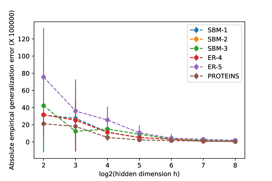
(b) MPGNN.

Figure 2: Absolute empirical generalization error ($\times 10^{5}$) for different widths $h$ of the hidden layer. We employ a mean-readout function and a supervised ratio of $\beta_{\text{sup}}=0.7,$ for GCN and MPGNN. Values are averaged over ten runs. Error bars indicate one standard deviation.

From Fig. 2 (and App. G with detailed mean and standard deviation values), we observe a consistent trend: as the value of $h$ increases, the absolute generalization error decreases. This observation shows that the upper bounds dependent on the width of the layer fail to capture the trend of generalization error in the over-parameterized regime. We provide extended actual absolute generalization errors in this section and the values of our upper bounds are provided in App. G.

7 Conclusions and Future Work

This work develops generalization error upper bounds for one-hidden-layer GCNs and MPGNNs for graph classification in the over-parameterized regime. Our analysis is based on a mean-field approach. Our upper bound on the generalization error of one-hidden-layer GCNs and MPGNNs with the KL-regularized empirical risk minimization is of the order of $O(1/n)$, where $n$ is the number of graph data samples, in the mean-field regime. This order is a significant improvement over previous work, see Table 1.

The main limitation of our work is that it considers only one hidden layer for graph convolutional networks and message-passing graph neural networks. Inspired by Sirignano and Spiliopoulos (2019), we aim to apply our approach to deep graph neural networks and investigate the effect of depth on the generalization performance. Furthermore, we plan to expand the current framework to study the generalization error of hypergraph neural networks, using the framework introduced in Feng et al. (2019).

Broader Impact Statement

This paper presents work whose goal is to advance the field of Machine Learning by providing a theoretical underpinning. There are many indirect potential societal consequences of our work through applications of empirical risk, see for example discussions in Abrahamsson and Johansson (2006) and Tran et al. (2021), and we believe that no direct consequences warrant being highlighted.

Appendix A Notation Summary

Notations in this paper are summarized in Table 2.

Table 2: Summary of notations in the paper

Notation	Definition	Notation	Definition
$\mathcal{W}$	Parameter space of the model	$\mathcal{F}$	Feature matrices space
$\mathcal{A}$	Adjacency matrices space	$\mathbf{F}$	Matrix of feature nodes of a graph sample
$\mathbf{A}$	Adjacency matrix of a graph sample	$\mathbf{X}$	input graph sample where $\mathbf{X}=(\mathbf{A},\mathbf{F})$
$Y$	Label of input graph	$Z_{i}$	$i$-th graph sample $(\mathbf{X},Y)$
$\mathbf{Z}_{n}$	The set of data training samples	$D$	Degree matrix of $A$
$\tilde{L}$	Symmetric normalized graph filter	$n$	Number of graph data samples
$N_{\max}$	Maximum number of nodes of all graph samples	$d_{\max}$	Maximum node degree of all graph samples
$d_{\min}$	Minimum node degree of all graph samples	$G(\mathbf{A})$	Graph filter with input matrix $\mathbf{A}$
$\mu_{n}$	Empirical data measure	$\mu_{n,(1)}$	Replace-one sample empirical data measure
$M_{\phi}$	Bound on unit function	$M_{\ell^{\prime}}$	Bound on $|\partial_{\hat{y}}\ell(\hat{y},y)|$
$L_{\zeta}$	Lipschitz parameter of function $\zeta(\cdot)$	$L_{\rho}$	Lipschitz parameter of function $\rho(\cdot)$
$L_{\kappa}$	Lipschitz parameter of function $\kappa(\cdot)$	$L_{\psi}$	Lipschitz parameter of readout function $\psi(\cdot)$
$L_{\varphi}$	Lipschitz parameter of activation function $\psi(\cdot)$	$B_{f}$	Bound on node features
$\alpha$	Inverse temperature	$h$	Width of hidden layer
$\pi$	Prior measure over parameters	$\mathrm{m}^{\alpha}$	The Gibbs measure for General GNN model
$\mathrm{m}^{\alpha,c}$	The Gibbs measure for GCN model	$\mathrm{m}^{\alpha,p}$	The Gibbs measure for MPGNN model
$m_{\mathrm{true}}$	True distribution over data samples	$G_{\max}$	$\min(\norm{G(\mathcal{A})}_{\infty}^{\max},\norm{G(\mathcal{A})}_{F}^{\max})$
$\Psi(\cdot)$	Readout function	$(W_{1,c},W_{2,c})$	Parameters of Neuron unit
$(W_{1,p},W_{2,p},W_{3,p})$	Parameters of MPU unit	$\overline{\mathrm{gen}}(\mathrm{m}(\mu_{n}),\mu)$	Generalization error under parameter measure $\mathrm{m}(\mu_{n})$
$\beta_{\mathrm{sup}}$	Supervised ratio	$\norm{\mathbf{Y}}_{F}$	$\sqrt{\sum_{j=1}^{k}\sum_{i=1}^{q}\mathbf{Y}^{2}[j,i]}$
$\norm{\mathbf{Y}}_{\infty}$	$\max_{1\leq j\leq k}\sum_{i=1}^{q}|\mathbf{Y}[j,i]|$	$\mathrm{KL}(p\|q)$	$\int_{\mathbb{R}^{d}}p(x)\log(p(x)/q(x))\mathrm{d}x$
$\mathrm{KL}_{\mathrm{sym}}(p\|q)$	$\mathrm{KL}(p\|q)+\mathrm{KL}(q\|p)$	$\phi(\cdot)$	Unit function

Appendix B Theoretical Preliminaries

Let us recapitulate all the assumptions required for our proofs.

Assumption 5.1 (Loss function).

The loss function, $(\hat{y},y)\mapsto\ell(\hat{y},y)$, satisfies the following conditions,

1. The gradient of the loss function $(\hat{y},y)\mapsto\ell(\hat{y},y)$ with respect to $\hat{y}$ is continuous and uniformly bounded for all $\hat{y},y\in\mathcal{Y}$, i.e., there is a constant $M_{\ell^{\prime}}$ such that $|\partial_{\hat{y}}\ell(\hat{y},y)|\leq M_{\ell^{\prime}}.$

2. We assume that the loss function is convex with respect to $\hat{y}$.

Assumption 5.2 (Bounded loss function).

The loss function, $(\hat{y},y)\mapsto\ell(\hat{y},y)$, is bounded for all $\hat{y},y\in\mathcal{Y}$, i.e., $0\leq\ell(\hat{y},y)\leq M_{\ell}$.

Assumption 5.3 (Unit function).

The unit function $(w,G(\mathbf{A})[j,:]\mathbf{f})\mapsto\phi(w,G(\mathbf{A})[j,:]\mathbf{f})$ with graph filter $G(\cdot)$ is uniformly bounded, i.e, there is a constant $M_{\phi}$ such that $\sup_{w\in\mathcal{W},\mathbf{f}\in\mathcal{F},\mathbf{A}\in\mathcal{A}}|\phi(w,G(\mathbf{A})[j,:]\mathbf{f})|\leq M_{\phi}$ for all $j\in[N]$ and $\mathbf{f}\in\mathcal{F}$.

Assumption 5.4 (Readout function).

The function $\psi:\mathbb{R}\mapsto\mathbb{R}$ is $L_{\psi}$-Lipschitz-continuous, i.e., there is a constant $L_{\psi}$ such that $|\psi(x_{1})-\psi(x_{2})|\leq L_{\psi}|x_{1}-x_{2}|$ for all $x_{1},x_{2}\in\mathbb{R}$, and zero-centered, i.e., $\psi(0)=0$.

Assumption 5.5 (Bounded node features).

For every graph, the node features are contained in an $\ell_{2}$-ball of radius $B_{f}$. In particular, $\norm{\mathbf{F}[i;]}_{2}\leq B_{f}$ for all $i\in[N]$.

Assumption 5.16 (Activation functions in neuron unit).

The activation function $\varphi:\mathbb{R}\mapsto\mathbb{R}$ is $L_{\varphi}$-Lipschitz, so that $|\varphi(x_{1})-\varphi(x_{2})|\leq L_{\varphi}|x_{1}-x_{2}|$ for all $x_{1},x_{2}\in\mathbb{R}$, and zero-centered, i.e., $\phi(0)=0$.

Assumption 5.21 (Non-linear functions in the MPGNN unit).

The non-linear functions $\zeta:\mathbb{R}^{N\times k}\mapsto\mathbb{R}^{N\times k}$, $\rho:\mathbb{R}^{k}\mapsto\mathbb{R}^{k}$ and $\kappa:\mathbb{R}\mapsto\mathbb{R}$ are zero-centered, i.e., $\zeta(\boldsymbol{0}^{N\times k})=\boldsymbol{0}^{N\times k}$, $\rho(\boldsymbol{0}^{k})=\boldsymbol{0}^{k}$ and $\kappa(0)=0$, and Lipschitz with parameters $L_{\zeta}$, $L_{\rho}$ and $L_{\kappa}$ under vector 2-norm, respectively.

Total variation distance: The total variation distance between two densities $p(x)$ and $q(x)$, is defined as $\mathbb{TV}(p,q):=\frac{1}{2}\int_{\mathbb{R}^{d}}|p(x)-q(x)|\mathrm{d}x$.

The following lemmas are needed for our proofs.

Lemma B.1 (Donsker’s representation of KL divergence).

Let us consider the variational representation of the KL divergence between two probability distributions $m_{1}$ and $m_{2}$ on a common space $\psi$ given by Polyanskiy and Wu (2022),

$$\mathrm{KL}(m_{1}||m_{2})=\sup_{f}\int_{\psi}fdm_{1}-\log\int_{\psi}e^{f}dm_{2},$$ (14)

where $f\in\mathfrak{F}=\{f:\psi\rightarrow\mathbb{R}\text{ s.t. }\mathbb{E}_{m_{2}}[e^{f}]<\infty\}$.

Lemma B.2 (Kantorovich-Rubenstein duality of total variation distance).

The Kantorovich-Rubenstein duality (variational representation) of the total variation distance is as follows Polyanskiy and Wu (2022):

$$\mathbb{TV}(m_{1},m_{2})=\frac{1}{2L}\sup_{g\in\mathcal{G}_{L}}\left\{\mathbb{E}_{Z\sim m_{1}}[g(Z)]-\mathbb{E}_{Z\sim m_{2}}[g(Z)]\right\},$$ (15)

where $\mathcal{G}_{L}=\{g:\mathcal{Z}\rightarrow\mathbb{R},||g||_{\infty}\leq L\}$.

Lemma B.3 (Bound on infinite norm of the symmetric normalized graph filter).

Consider a graph sample $G$ with adjacency matrix $A$. For the symmetric normalized graph filter, we have $\norm{\tilde{D}^{-1/2}(A+I)\tilde{D}^{-1/2}}_{\infty}\leq\sqrt{\frac{d_{\max}+1}{d_{\min}+1}}$ where $d_{\max}$ is the maximum degree of graph $G$ with adjacency matrix $A$.

Proof.

Recall that $\tilde{A}=A+I$. We have,

$$\begin{split}\norm{\tilde{L}}_{\infty}&=\norm{\tilde{D}^{-1/2}\tilde{A}\tilde{D}^{-1/2}}_{\infty}\\ &=\max_{i\in[N]}\sum_{j=1}^{N}\frac{\tilde{A}_{ij}}{\sqrt{d_{i}+1}\sqrt{d_{j}+1}}\\ &\leq\frac{1}{\sqrt{d_{\min}+1}}\max_{i\in[N]}\sum_{j=1}^{N}\frac{\tilde{A}_{ij}}{\sqrt{d_{i}+1}}\\ &\leq\sqrt{\frac{d_{\max}+1}{d_{\min}+1}}.\end{split}$$ (16)

∎

Lemma B.4 (Meyer and Stewart, 2023).

For a matrix $\mathbf{Y}\in\mathbb{R}^{k\times q}$, we have $\norm{\mathbf{Y}}_{F}\leq\sqrt{R}\norm{\mathbf{Y}}_{2}$, where $r$ is the rank of $\mathbf{Y}$ and $\norm{\mathbf{Y}}_{2}$ is the 2-norm of $\mathbf{Y}$ which is equal to the maximum singular value of $\mathbf{Y}$.

Lemma B.5 (Verma and Zhang, 2019).

For the symmetric normalized graph filter, i.e., $\tilde{L}=\tilde{D}^{-1/2}\tilde{\mathbf{A}}\tilde{D}^{-1/2}$, we have $\norm{\tilde{L}}_{2}=1$. For the random walk graph filter, i.e., $D^{-1}\mathbf{A}+I$, we have $\norm{D^{-1}\mathbf{A}+I}_{2}=2$, where $\norm{A}_{2}$ is the 2-norm of matrix A.

Lemma B.6 (Hoeffding lemma Wainwright (2019)).

For bounded random variable, $a\leq X\leq b$, and all $\lambda\in\mathbb{R}$, we have,

$$\mathbb{E}[\exp(\lambda(X-\mathbb{E}[X]))]\leq\exp(\lambda(b-a)^{2}/8).$$ (17)

Lemma B.7 (Pinsker’s inequality).

The following upper bound holds on the total variation distance between two measures $m_{1}$ and $m_{2}$ Polyanskiy and Wu (2022):

$$\mathbb{TV}(m_{1},m_{2})\leq\sqrt{\frac{\mathrm{KL}(m_{1}\|m_{2})}{2}}.$$ (18)

In the following, we apply some lemmata from Aminian et al. (2023) where we use $\ell\big{(}\Psi(\mathrm{m}(\mu_{n}),\,\widehat{\!{\mathbf{x}}}_{1}),\,\widehat{\!{\mathbf{y}}}_{1}\big{)}$ instead of $\ell\big{(}\mathrm{m}(\mu_{n}),\,\widehat{\!{Z}}_{1}\big{)}$ in Aminian et al. (2023).

Lemma B.8.

(Aminian et al., 2023, Proposition 3.3) Given Assumption 5.1, the following lower bound holds on the generalization error of a Generic GNN,

$$\overline{\mathrm{gen}}(\mathrm{m}^{\alpha}(\mu_{n}),\mu)\geq\mathbb{E}_{\mathbf{Z}_{n},\,\widehat{\!{Z}}_{1}}\Big{[}\int_{\mathcal{W}}\partial_{\hat{y}}\ell\big{(}\Psi(\mathrm{m}(\mu_{n,(1)}),\,\widehat{\!{\mathbf{x}}}_{1}),\,\widehat{\!{\mathbf{y}}}_{1}\big{)}\frac{\delta\Psi}{\delta\mathrm{m}}(\mathrm{m}(\mu_{n,(1)}),\,\widehat{\!{\mathbf{x}}}_{1},w)(\mathrm{m}(\mu_{n})-\mathrm{m}(\mu_{n,(1)}))(\mathrm{d}w)\Big{]}.$$

Remark B.9 (Another representation of Lemma B.8).

Due to the fact that data samples and $\,\widehat{\!{Z}}_{1}$ are i.i.d., Lemma B.8 can be represented as follows,

$$\overline{\mathrm{gen}}(\mathrm{m}^{\alpha}(\mu_{n}),\mu)\geq\mathbb{E}_{\mathbf{Z}_{n},\,\widehat{\!{Z}}_{1}}\Big{[}\int_{\mathcal{W}}\partial_{\hat{y}}\ell\big{(}\Psi(\mathrm{m}(\mu_{n}),\mathbf{x}_{1}),\mathbf{y}_{1}\big{)}\frac{\delta\Psi}{\delta\mathrm{m}}(\mathrm{m}(\mu_{n}),\mathbf{x}_{1},w)(\mathrm{m}(\mu_{n,(1)})-\mathrm{m}(\mu_{n}))(\mathrm{d}w)\Big{]}.$$

Lemma B.10.

(Aminian et al., 2023, Theorem 3.2) Given Assumption 5.1.i, the following representation of the generalization error holds:

$$\overline{\mathrm{gen}}(\mathrm{m}^{\alpha}(\mu_{n}),\mu)=\mathbb{E}_{\mathbf{Z}_{n},\,\widehat{\!{Z}}_{1}}\Big{[}\int_{0}^{1}\int_{\mathcal{W}}\partial_{\hat{y}}\ell\big{(}\Psi(\mathrm{m}_{\lambda}(\mu_{n}),\,\widehat{\!{\mathbf{x}}}_{1}),\,\widehat{\!{\mathbf{y}}}_{1}\big{)}\frac{\delta\Psi}{\delta\mathrm{m}}(\mathrm{m}_{\lambda}(\mu_{n}),\,\widehat{\!{\mathbf{x}}}_{1},w)(\mathrm{m}(\mu_{n})-\mathrm{m}(\mu_{n,(1)}))(\mathrm{d}w)\mathrm{d}\lambda\Big{]}$$

where $\mathrm{m}_{\lambda}(\mu_{n})=\mathrm{m}(\mu_{n,(1)})+\lambda(\mathrm{m}(\mu_{n})-\mathrm{m}(\mu_{n,(1)}))$ for $\lambda\in[0,1]$.

The following preliminaries are needed for our Rademacher complexity analysis.

Rademacher complexity: For a hypothesis set, $\mathcal{H}$ of functions $f_{h}:\mathcal{Z}\mapsto\mathbb{R}$ and set $\boldsymbol{\sigma}=\{\sigma_{i}\}_{i=1}^{r}$, the empirical Rademacher complexity $\hat{\mathfrak{R}}_{\mathrm{Z}}(\mathcal{H})$ with respect to set $\mathbf{Z}_{n}$ is defined as:

$$\hat{\mathfrak{R}}_{\mathbf{Z}_{n}}(\mathcal{H}):=\mathbb{E}_{\boldsymbol{\sigma}}\Big{[}\sup_{f_{h}\in\mathcal{H}}\frac{1}{n}\sum_{i=1}^{r}\sigma_{i}f_{h}(Z_{i})\Big{]}\,,$$ (19)

where $\sigma=\{\sigma_{i}\}_{i=1}^{r}$ are i.i.d random variables and $\sigma_{i}\in\{-1,1\}$ for all $i\in[r]$ with equal probability.

Lemma B.11 (Uniform bound Mohri et al. (2018)).

Let $\mathcal{F}_{u}$ be the set of functions $f:\mathcal{Z}\to[0,M_{\ell}]$ and $\mu$ be a distribution over $\mathcal{Z}$. Let $S=\{z_{i}\}_{i=1}^{r}$ be a set of size $r$ i.i.d. drawn from $\mathcal{Z}$. Then, for any $\delta\in(0,1)$, with probability at least $1-\delta$ over the choice of $S$, we have

$$\sup_{f\in\mathcal{F}_{u}}\left\{\mathbb{E}_{Z\sim\mu}[f(Z)]-\frac{1}{n}\sum_{i=1}^{r}f(z_{i})\right\}\leq 2\hat{\mathfrak{R}}_{S}(\mathcal{F}_{u})+3M_{\ell}\sqrt{\frac{1}{2n}\log\frac{2}{\delta}}.$$

The contraction lemma helps us to estimate the Rademacher complexity.

Lemma B.12 (Talagrand’s contraction lemma (Shalev-Shwartz and Ben-David, 2014)).

Let $\phi_{i}:\mathbb{R}\rightarrow\mathbb{R}$ $(i\in\{1,\ldots,r\})$ be $L$-Lipschitz functions and $\mathcal{F}_{r}$ be a set of functions from $\mathcal{Z}$ to $\mathbb{R}$. Then it follows that for any $\{z_{i}\}_{i=1}^{r}\subset\mathcal{Z}$,

$$\mathbb{E}_{\sigma}\left[\sup_{f\in\mathcal{F}_{r}}\frac{1}{n}\sum_{i=1}^{r}\sigma_{i}\phi_{i}(f(z_{i}))\right]\leq L\mathbb{E}_{\sigma}\left[\sup_{f\in\mathcal{F}_{r}}\frac{1}{n}\sum_{i=1}^{r}\sigma_{i}f(z_{i})\right].$$

Appendix C Other Related Works

Mean-field: Our study employs the mean-field framework utilized in a recent line of research Chizat and Bach (2018); Mei et al. (2018, 2019); Sirignano and Spiliopoulos (2019); Hu et al. (2019). The convergence of gradient descent for training one-hidden layer NNs with infinite width under certain structural assumptions is established by Chizat and Bach (2018). The study of Mei et al. (2018) proved the global convergence of noisy stochastic gradient descent and established approximation bounds between finite and infinite neural networks. Furthermore, Mei et al. (2019) demonstrated that this approximation error can be independent of the input dimension in certain cases, and established that the residual dynamics of noiseless gradient descent are close to the dynamics of NTK-based kernel regression under some conditions.

Graph Representation Learning: Numerous Graph Neural Networks (GNNs) have emerged for graph-based tasks, spanning node, edge, and graph levels. GCNs, introduced in Kipf and Welling (2016), simplify the Cheby-Filter from Defferrard et al. (2016) for one-hop neighbors. MPGNNs, as proposed in Gilmer et al. (2017), outline a general GNN framework, treating graph convolutions as message-passing among nodes and edges. For graph-level tasks, like graph classification, a typical practice involves applying a graph readout (pooling) layer after graph filtering layers, composed of graph filters. The readout (pooling) layer aggregates node representations to create a graph-wide embedding. Common graph readout choices encompass set pooling methods like direct sum application, mean (Hamilton, 2020), or maximum (Mesquita et al., 2020), as well as combinations of LSTMs with attention (Vinyals et al., 2015) and graph coarsening techniques leveraging graph structure (Ying et al., 2018b; Cangea et al., 2018; Gao and Ji, 2019). In this paper, we investigate how mean and sum impact the generalization errors of GCNs and MPGNNs.

Node Classification and Generalization Error: For node classification tasks, Verma and Zhang (2019) discussed the generalization error under node classification for GNNs via algorithm stability analysis. The work by Zhou and Wang (2021) extended the results in Verma and Zhang (2019) and found that increasing the depth of GCN enlarges its generalization error for the node classification task. A Rademacher complexity analysis was applied to GCNs for the node classification task by Lv (2021). Based on transductive Rademacher complexity, a high-probability upper bound on the generalization error of the transductive node classification task was proposed by Esser et al. (2021). The transductive modeling of node classification was studied in Oono and Suzuki (2020) and Tang and Liu (2023). Cong et al. (2021) presented an upper bound on the generalization error of GCNs for node classification via transductive uniform stability, building on the work of El-Yaniv and Pechyony (2006). In contrast, our research focuses on the task of graph classification, which involves (semi-)supervised learning on graph data samples rather than semi-supervised learning for node classification.

Neural Tangent Kernels:The neural tangent kernel (NTK) model, as described by Jacot et al. (2018a), elucidates the learning dynamics inherent in neural networks when subjected to appropriate scaling conditions. This explication relies on the linearization of learning dynamics in proximity to its initialization. Conclusive evidence pertaining to the (quantitative) global convergence of gradient-based techniques for neural networks has been established for both regression problems Suzuki and Nitanda (2021) and classification problems Cao and Gu (2019). The NTK model, founded upon linearization, is constrained in its ability to account for the phenomenon of "feature learning" within neural networks, wherein parameters exhibit the capacity to traverse and adapt to the inherent structure of the learning problem. Fundamental to this analysis is the linearization of training dynamics, necessitating the imposition of appropriate scaling conditions on the model Chizat and Bach (1812). Consequently, this framework proves inadequate for elucidating the feature learning aspect of neural networks Yang and Hu (2020); Fang et al. (2021). Notably, empirical investigations have demonstrated the superior expressive power of deep learning over kernel methods concerning approximation and estimation errors Ghorbani et al. (2021). In certain contexts, it has been observed that neural networks, optimized through gradient-based methodologies, surpass the predictive performance of the NTK model, and more broadly, kernel methods, concerning generalization error or true risk Allen-Zhu and Li (2019).

Appendix D Proofs and details of Section 5

D.1 Generic GNN

Proposition 5.6.

(restated) Let Assumptions 5.1, 5.3, and 5.4 hold. Then, the following bound holds on the generalization error of generic GNN,

$$\begin{split}&\Big{|}\overline{\mathrm{gen}}(\mathrm{m}(\mu_{n}),\mu)\Big{|}\leq\big{(}M_{\ell^{\prime}}L_{\psi}N_{\max}M_{\phi}/\sqrt{2}\big{)}\mathbb{E}_{\mathbf{Z}_{n},\,\widehat{\!{Z}}_{1}}\Big{[}\sqrt{\mathrm{KL}\big{(}\mathrm{m}(\mu_{n})\|\mathrm{m}(\mu_{n,(1)})\big{)}}\Big{]}.\end{split}$$ (20)

In the following, we provide two technical proofs for Proposition 5.6.

Proof of Proposition 5.6 via Lemma B.1 and Lemma B.6.

From Lemma B.1, the following representation of KL divergence holds between two probability distributions $m_{1}$ and $m_{2}$ on a common space $\mathcal{W}$,

$$\mathrm{KL}(m_{1}\|m_{2})=\sup_{f\in\mathfrak{F}}\mathbb{E}_{W\sim m_{1}}[f(W)]-\log{\big{(}\mathbb{E}_{W\sim m_{2}}[\exp{f(W)}]\big{)}},$$ (21)

where $f\in\mathfrak{F}=\{f:\mathcal{W}\rightarrow\mathbb{R}\text{ s.t. }\mathbb{E}_{W\sim m_{2}}[e^{f(W)}]<\infty\}$. Lemma B.10 yields

$$\begin{split}&\overline{\mathrm{gen}}(\mathrm{m}^{\alpha}(\mu_{n}),\mu)\\ &=\mathbb{E}_{\mathbf{Z}_{n},\,\widehat{\!{Z}}_{1}}\Big{[}\int_{0}^{1}\int_{\mathcal{W}}\partial_{\hat{y}}\ell\big{(}\Psi(\mathrm{m}_{\lambda}(\mu_{n}),\,\widehat{\!{\mathbf{x}}}_{1}),\,\widehat{\!{\mathbf{y}}}_{1}\big{)}\frac{\delta\Psi}{\delta\mathrm{m}}(\mathrm{m}_{\lambda}(\mu_{n}),\,\widehat{\!{\mathbf{x}}}_{1},w)(\mathrm{m}(\mu_{n})-\mathrm{m}(\mu_{n,(1)}))(\mathrm{d}w)\mathrm{d}\lambda\Big{]}\\ &=\mathbb{E}_{\mathbf{Z}_{n},\,\widehat{\!{Z}}_{1}}\Big{[}\int_{0}^{1}\partial_{\hat{y}}\ell\big{(}\Psi(\mathrm{m}_{\lambda}(\mu_{n}),\,\widehat{\!{\mathbf{x}}}_{1}),\,\widehat{\!{\mathbf{y}}}_{1}\big{)}\Big{(}\mathbb{E}_{W\sim\mathrm{m}(\mu_{n})}\Big{[}\frac{\delta\Psi}{\delta\mathrm{m}}(\mathrm{m}_{\lambda}(\mu_{n}),\,\widehat{\!{\mathbf{x}}}_{1},W)\Big{]}\\ &\qquad\qquad-\mathbb{E}_{W\sim\mathrm{m}(\mu_{n,(1)})}\Big{[}\frac{\delta\Psi}{\delta\mathrm{m}}(\mathrm{m}_{\lambda}(\mu_{n}),\,\widehat{\!{\mathbf{x}}}_{1},W)\Big{]}\Big{)}\mathrm{d}\lambda\Big{]}.\end{split}$$

For the function $f(w)=\lambda_{1}\partial_{\hat{y}}\ell\big{(}\Psi(\mathrm{m}_{\lambda}(\mu_{n}),\,\widehat{\!{\mathbf{x}}}_{1}),\,\widehat{\!{\mathbf{y}}}_{1}\big{)}\frac{\delta\Psi}{\delta\mathrm{m}}(\mathrm{m}_{\lambda}(\mu_{n}),\,\widehat{\!{\mathbf{x}}}_{1},w)$, due to Assumptions 5.1, 5.3 and 5.4, we have $\Big{|}\partial_{\hat{y}}\ell\big{(}\Psi(\mathrm{m}_{\lambda}(\mu_{n}),\,\widehat{\!{\mathbf{x}}}_{1}),\,\widehat{\!{\mathbf{y}}}_{1}\big{)}\frac{\delta\Psi}{\delta\mathrm{m}}(\mathrm{m}_{\lambda}(\mu_{n}),\,\widehat{\!{\mathbf{x}}}_{1},w)\Big{|}\leq M_{\ell^{\prime}}L_{\psi}N_{\max}M_{\phi}$. Hence $f\in\mathfrak{F}$.

From (21), for $m_{1}=\mathrm{m}(\mu_{n})$ and $m_{2}=\mathrm{m}(\mu_{n,(1)})$, we have for all $\lambda_{1}\in\mathbb{R}$

$$\lambda_{1}\mathbb{E}_{W\sim\mathrm{m}(\mu_{n})}\Big{[}\Big{(}\partial_{\hat{y}}\ell\big{(}\Psi(\mathrm{m}_{\lambda}(\mu_{n}),\,\widehat{\!{\mathbf{x}}}_{1})],\,\widehat{\!{\mathbf{y}}}_{1}\big{)}\frac{\delta\Psi}{\delta\mathrm{m}}(\mathrm{m}_{\lambda}(\mu_{n}),\,\widehat{\!{\mathbf{x}}}_{1},W)\Big{)}\Big{]}$$ (22)

$$\leq\mathrm{KL}(\mathrm{m}(\mu_{n})\|\mathrm{m}(\mu_{n,(1)}))+\log\Big(\mathbb{E}_{W\sim\mathrm{m}^{\alpha}(\mu_{n,(1)})}\Big{[}\exp\{\lambda_{1}\Big{(}\partial_{\hat{y}}\ell\big{(}\Psi(\mathrm{m}_{\lambda}(\mu_{n}),\,\widehat{\!{\mathbf{x}}}_{1}),\,\widehat{\!{\mathbf{y}}}_{1}\big{)}\frac{\delta\Psi}{\delta\mathrm{m}}(\mathrm{m}_{\lambda}(\mu_{n}),\,\widehat{\!{\mathbf{x}}}_{1},W)\Big{)}\Big{\}}\Big{]}\Big{missing}).$$

With Lemma B.6,

$$\begin{split}&\mathbb{E}_{W\sim\mathrm{m}^{\alpha}(\mu_{n,(1)})}\Big{[}\exp\{\lambda_{1}\Big{(}\partial_{\hat{y}}\ell\big{(}\Psi(\mathrm{m}_{\lambda}(\mu_{n}),\,\widehat{\!{\mathbf{x}}}_{1}),\,\widehat{\!{\mathbf{y}}}_{1}\big{)}\Big{(}\frac{\delta\Psi}{\delta\mathrm{m}}(\mathrm{m}_{\lambda}(\mu_{n}),\,\widehat{\!{\mathbf{x}}}_{1},W)-\\ &\qquad\qquad\qquad\mathbb{E}_{W\sim\mathrm{m}^{\alpha}(\mu_{n,(1)})}\Big{[}\frac{\delta\Psi}{\delta\mathrm{m}}(\mathrm{m}_{\lambda}(\mu_{n}),\,\widehat{\!{\mathbf{x}}}_{1},W)\Big{]}\Big{)}\Big{)}\Big{\}}\Big{]}\\ &\quad\leq\exp{\frac{\lambda_{1}^{2}\sigma_{1}^{2}}{2}},\end{split}$$ (23)

where $\sigma_{1}=M_{\ell^{\prime}}L_{\psi}N_{\max}M_{\phi}$. Combining (23) with (22), we can derive the following:

$$\lambda_{1}\Big{(}\partial_{\hat{y}}\ell\big{(}\Psi(\mathrm{m}_{\lambda}(\mu_{n}),\,\widehat{\!{\mathbf{x}}}_{1}),\,\widehat{\!{\mathbf{y}}}_{1}\big{)}\Big{(}\mathbb{E}_{W\sim\mathrm{m}(\mu_{n})}\Big{[}\frac{\delta\Psi}{\delta\mathrm{m}}(\mathrm{m}_{\lambda}(\mu_{n}),\,\widehat{\!{\mathbf{x}}}_{1},W)\Big{]}-\mathbb{E}_{W\sim\mathrm{m}(\mu_{n,(1)})}\Big{[}\frac{\delta\Psi}{\delta\mathrm{m}}(\mathrm{m}_{\lambda}(\mu_{n}),\,\widehat{\!{\mathbf{x}}}_{1},W)\Big{]}\Big{)}\Big{)}$$

$$\leq\mathrm{KL}(\mathrm{m}(\mu_{n})\|\mathrm{m}(\mu_{n,(1)}))+\frac{\lambda_{1}^{2}\sigma_{1}^{2}}{2},$$

This is a nonnegative parabola in $\lambda_{1}$, whose discriminant must be nonpositive. Therefore, we have,

$$\begin{split}&\Big{|}\partial_{\hat{y}}\ell\big{(}\Psi(\mathrm{m}_{\lambda}(\mu_{n}),\,\widehat{\!{\mathbf{x}}}_{1}),\,\widehat{\!{\mathbf{y}}}_{1}\big{)}\Big{(}\mathbb{E}_{W\sim\mathrm{m}(\mu_{n})}\Big{[}\frac{\delta\Psi}{\delta\mathrm{m}}(\mathrm{m}_{\lambda}(\mu_{n}),\,\widehat{\!{\mathbf{x}}}_{1},W)\Big{]}-\mathbb{E}_{W\sim\mathrm{m}(\mu_{n,(1)})}\Big{[}\frac{\delta\Psi}{\delta\mathrm{m}}(\mathrm{m}_{\lambda}(\mu_{n}),\,\widehat{\!{\mathbf{x}}}_{1},W)\Big{]}\Big{)}\Big{|}\\ &\leq\sqrt{2\sigma_{1}^{2}\mathrm{KL}(\mathrm{m}(\mu_{n})\|\mathrm{m}(\mu_{n,(1)}))}.\end{split}$$ (24)

The upper bound in (24) holds for all $\lambda\in[0,1]$. Therefore, combining with Lemma B.10, we have,

$$\begin{split}&\overline{\mathrm{gen}}(\mathrm{m}^{\alpha}(\mu_{n}),\mu)\\ &=\mathbb{E}_{\mathbf{Z}_{n},\,\widehat{\!{Z}}_{1}}\Big{[}\int_{0}^{1}\partial_{\hat{y}}\ell\big{(}\Psi(\mathrm{m}_{\lambda}(\mu_{n}),\,\widehat{\!{\mathbf{x}}}_{1}),\,\widehat{\!{\mathbf{y}}}_{1}\big{)}\Big{(}\mathbb{E}_{W\sim\mathrm{m}(\mu_{n})}\Big{[}\frac{\delta\Psi}{\delta\mathrm{m}}(\mathrm{m}_{\lambda}(\mu_{n}),\,\widehat{\!{\mathbf{x}}}_{1},W)\Big{]}\\ &\qquad\qquad\qquad-\mathbb{E}_{W\sim\mathrm{m}(\mu_{n,(1)})}\Big{[}\frac{\delta\Psi}{\delta\mathrm{m}}(\mathrm{m}_{\lambda}(\mu_{n}),\,\widehat{\!{\mathbf{x}}}_{1},W)\Big{]}\Big{)}\mathrm{d}\lambda\Big{]}\\ \\ &\leq\mathbb{E}_{\mathbf{Z}_{n},\,\widehat{\!{Z}}_{1}}\Bigg{[}\int_{0}^{1}\Big{|}\partial_{\hat{y}}\ell\big{(}\Psi(\mathrm{m}_{\lambda}(\mu_{n}),\,\widehat{\!{\mathbf{x}}}_{1}),\,\widehat{\!{\mathbf{y}}}_{1}\big{)}\Big{(}\mathbb{E}_{W\sim\mathrm{m}(\mu_{n})}\Big{[}\frac{\delta\Psi}{\delta\mathrm{m}}(\mathrm{m}_{\lambda}(\mu_{n}),\,\widehat{\!{\mathbf{x}}}_{1},W)\Big{]}\\ &\qquad\qquad\qquad-\mathbb{E}_{W\sim\mathrm{m}(\mu_{n,(1)})}\Big{[}\frac{\delta\Psi}{\delta\mathrm{m}}(\mathrm{m}_{\lambda}(\mu_{n}),\,\widehat{\!{\mathbf{x}}}_{1},W)\Big{]}\Big{)}\Big{|}\mathrm{d}\lambda\Bigg{]}\\ &\leq\mathbb{E}_{\mathbf{Z}_{n},\,\widehat{\!{Z}}_{1}}\Big{[}\sqrt{2\sigma_{1}^{2}\mathrm{KL}(\mathrm{m}(\mu_{n})\|\mathrm{m}(\mu_{n,(1)}))}\Big{]}.\end{split}$$ (25)

This completes the proof. ∎

Proof of Proposition 5.6 via Lemma B.2 and Lemma B.7.

From Lemma B.10, it yields,

$$\begin{split}&\overline{\mathrm{gen}}(\mathrm{m}^{\alpha}(\mu_{n}),\mu)\\ &=\mathbb{E}_{\mathbf{Z}_{n},\,\widehat{\!{Z}}_{1}}\Big{[}\int_{0}^{1}\int_{\mathcal{W}}\partial_{\hat{y}}\ell\big{(}\Psi(\mathrm{m}_{\lambda}(\mu_{n}),\,\widehat{\!{\mathbf{x}}}_{1}),\,\widehat{\!{\mathbf{y}}}_{1}\big{)}\frac{\delta\Psi}{\delta\mathrm{m}}(\mathrm{m}_{\lambda}(\mu_{n}),\,\widehat{\!{\mathbf{x}}}_{1},w)(\mathrm{m}(\mu_{n})-\mathrm{m}(\mu_{n,(1)}))(\mathrm{d}w)\mathrm{d}\lambda\Big{]}\\ &=\mathbb{E}_{\mathbf{Z}_{n},\,\widehat{\!{Z}}_{1}}\Big{[}\int_{0}^{1}\partial_{\hat{y}}\ell\big{(}\Psi(\mathrm{m}_{\lambda}(\mu_{n}),\,\widehat{\!{\mathbf{x}}}_{1}),\,\widehat{\!{\mathbf{y}}}_{1}\big{)}\Big{(}\mathbb{E}_{W\sim\mathrm{m}(\mu_{n})}\Big{[}\frac{\delta\Psi}{\delta\mathrm{m}}(\mathrm{m}_{\lambda}(\mu_{n}),\,\widehat{\!{\mathbf{x}}}_{1},W)\Big{]}\\ &\qquad\qquad\qquad-\mathbb{E}_{W\sim\mathrm{m}(\mu_{n,(1)})}\Big{[}\frac{\delta\Psi}{\delta\mathrm{m}}(\mathrm{m}_{\lambda}(\mu_{n}),\,\widehat{\!{\mathbf{x}}}_{1},W)\Big{]}\Big{)}\mathrm{d}\lambda\Big{]}.\end{split}$$

For the function $f(w)=\lambda_{1}\partial_{\hat{y}}\ell\big{(}\Psi(\mathrm{m}_{\lambda}(\mu_{n}),\,\widehat{\!{\mathbf{x}}}_{1}),\,\widehat{\!{\mathbf{y}}}_{1}\big{)}\frac{\delta\Psi}{\delta\mathrm{m}}(\mathrm{m}_{\lambda}(\mu_{n}),\,\widehat{\!{\mathbf{x}}}_{1},w)$, due to Assumptions 5.1, 5.3 and 5.4, we have $\Big{|}\partial_{\hat{y}}\ell\big{(}\Psi(\mathrm{m}_{\lambda}(\mu_{n}),\,\widehat{\!{\mathbf{x}}}_{1}),\,\widehat{\!{\mathbf{y}}}_{1}\big{)}\frac{\delta\Psi}{\delta\mathrm{m}}(\mathrm{m}_{\lambda}(\mu_{n}),\,\widehat{\!{\mathbf{x}}}_{1},w)\Big{|}\leq M_{\ell^{\prime}}L_{\psi}N_{\max}M_{\phi}$. Hence, from lemma B.2, it yields,

$$\big{|}\overline{\mathrm{gen}}(\mathrm{m}^{\alpha}(\mu_{n}),\mu)\big{|}\leq M_{\ell^{\prime}}L_{\psi}N_{\max}M_{\phi}\mathbb{E}_{\mathbf{Z}_{n},\,\widehat{\!{Z}}_{1}}\Big{[}\mathbb{TV}(\mathrm{m}(\mu_{n}),\mathrm{m}(\mu_{n,(1)}))\Big{]}.$$ (26)

Using Lemma B.7 completes the proof. ∎

Proposition 5.8.

(restated) Let Assumptions 5.1 hold. Then, the following lower bound holds on the generalization error of the Gibbs measure $m^{\alpha}(\mu_{n})$,

$$\begin{split}&\overline{\mathrm{gen}}(\mathrm{m}^{\alpha}(\mu_{n}),\mu)\geq\frac{n}{2\alpha}\mathbb{E}_{\mathbf{Z}_{n},\,\widehat{\!{Z}}_{1}}\Big{[}\mathrm{KL}_{\mathrm{sym}}\big{(}\mathrm{m}^{\alpha}(\mu_{n})\|\mathrm{m}^{\alpha}(\mu_{n,(1)})\big{)}\Big{]}.\end{split}$$

Proof.

For simplicity of proof, we abbreviate

$$\tilde{\ell}\big{(}m,z\big{)} :=\ell\big{(}\Psi(m,x),y\big{)},$$ (27)

$$\frac{\delta\tilde{\ell}}{\delta m}\big{(}m,z,w\big{)} :=\partial_{\hat{y}}\ell(\Psi(m,x),y)\frac{\delta\Psi}{\delta m}(m,x,w),$$ (28)

where $z=(x,y)$ and (28) follows from chain rule. From Assumption 5.1, where the loss function is convex with respect to $\Psi(m,x)$ and due to the fact that $\Psi(m,x)$ is linear with respect to parameter measure $m$, then we have the convexity of $\tilde{\ell}\big{(}m,z\big{)}$ with respect to parameter measure. Recall that from (11) we have

$$\mathrm{m}^{\alpha}(\mu_{n})=\frac{\pi}{S_{\alpha,\pi}(\mu_{n})}\exp\{-\alpha\Bigg{[}\frac{\delta\mathrm{R}(\mathrm{m}^{\alpha},\mu_{n},w)}{\delta m}\Bigg{]}\Bigg{\}},$$

and

$$\mathrm{m}^{\alpha}(\mu_{n,(1)})=\frac{\pi}{S_{\alpha,\pi}(\mu_{n,(1)})}\exp\{-\alpha\Bigg{[}\frac{\delta\mathrm{R}(\mathrm{m}^{\alpha},\mu_{n,(1)},w)}{\delta m}\Bigg{]}\Bigg{\}}.$$

We need to compute the expectation of $\mathrm{KL}_{\mathrm{sym}}\big{(}\mathrm{m}^{\alpha}(\mu_{n,(1)})\|\mathrm{m}^{\alpha}(\mu_{n})\big{)}$ where $\mathrm{KL}_{\mathrm{sym}}(p\|q)=\mathrm{KL}(p\|q)+\mathrm{KL}(q\|p)$. For that purpose,

$$\mathbb{E}_{\mathbf{Z}_{n},\,\widehat{\!{Z}}_{1}}\Big{[}\mathrm{KL}\big{(}\mathrm{m}^{\alpha}(\mu_{n})\|\mathrm{m}^{\alpha}(\mu_{n,(1)})\big{)}+\mathrm{KL}\big{(}\mathrm{m}^{\alpha}(\mu_{n,(1)})\|\mathrm{m}^{\alpha}(\mu_{n})\big{)}\Big{]}$$

$$=\mathbb{E}_{\mathbf{Z}_{n},\,\widehat{\!{Z}}_{1}}\Big{[}\int_{\mathcal{W}}\log(\mathrm{m}^{\alpha}(\mu_{n})/\mathrm{m}^{\alpha}(\mu_{n,(1)}))(\mathrm{m}^{\alpha}(\mu_{n})-\mathrm{m}^{\alpha}(\mu_{n,(1)}))(\mathrm{d}w)\Big{]}$$

$$=\mathbb{E}_{\mathbf{Z}_{n},\,\widehat{\!{Z}}_{1}}\Big{[}\int_{\mathcal{W}}\log(S_{\alpha,\pi}(\mu_{n,(1)})/S_{\alpha,\pi}(\mu_{n}))(\mathrm{m}^{\alpha}(\mu_{n})-\mathrm{m}^{\alpha}(\mu_{n,(1)}))(\mathrm{d}w)\Big{]}$$

$$\quad+\mathbb{E}_{\mathbf{Z}_{n},\,\widehat{\!{Z}}_{1}}\Big{[}\mathbb{E}_{W\sim\mathrm{m}^{\alpha}(\mu_{n,(1)})}\Big{[}\pi(W)\Big{]}-\mathbb{E}_{W\sim\mathrm{m}^{\alpha}(\mu_{n})}\Big{[}\pi(W)\Big{]}\Big{]}$$

$$\quad+\alpha\Big{(}\mathbb{E}_{\mathbf{Z}_{n},\,\widehat{\!{Z}}_{1}}\Big{[}\mathbb{E}_{W\sim\mathrm{m}^{\alpha}(\mu_{n})}\Big{[}\frac{\delta\mathrm{R}}{\delta m}(\mathrm{m}^{\alpha}(\mu_{n,(1)}),\mu_{n,(1)},W)-\frac{\delta\mathrm{R}}{\delta m}(\mathrm{m}^{\alpha}(\mu_{n}),\mu_{n},W)\Big{]}\Big{]}$$

$$\quad-\mathbb{E}_{\mathbf{Z}_{n},\,\widehat{\!{Z}}_{1}}\Big{[}\mathbb{E}_{W\sim\mathrm{m}^{\alpha}(\mu_{n,(1)})}\Big{[}\frac{\delta\mathrm{R}}{\delta m}(\mathrm{m}^{\alpha}(\mu_{n,(1)}),\mu_{n,(1)},W)-\frac{\delta\mathrm{R}}{\delta m}(\mathrm{m}^{\alpha}(\mu_{n}),\mu_{n},W)\Big{]}\Big{]}\Big{)}.$$

Let us define the following terms,

$$\begin{split}I_{1}&:=\mathbb{E}_{\mathbf{Z}_{n},\,\widehat{\!{Z}}_{1}}\Big{[}\int_{\mathcal{W}}\log(S_{\alpha,\pi}(\mu_{n,(1)})/S_{\alpha,\pi}(\mu_{n}))(\mathrm{m}^{\alpha}(\mu_{n})-\mathrm{m}^{\alpha}(\mu_{n,(1)}))(\mathrm{d}w)\Big{]},\\ I_{2}&:=\mathbb{E}_{\mathbf{Z}_{n},\,\widehat{\!{Z}}_{1}}\Big{[}\mathbb{E}_{W\sim\mathrm{m}^{\alpha}(\mu_{n,(1)})}\Big{[}\pi(W)\Big{]}-\mathbb{E}_{W\sim\mathrm{m}^{\alpha}(\mu_{n})}\Big{[}\pi(W)\Big{]}\Big{]},\\ I_{3}&:=\mathbb{E}_{\mathbf{Z}_{n},\,\widehat{\!{Z}}_{1}}\Big{[}\mathbb{E}_{W\sim\mathrm{m}^{\alpha}(\mu_{n})}\Big{[}\frac{\delta\mathrm{R}}{\delta m}(\mathrm{m}^{\alpha}(\mu_{n,(1)}),\mu_{n,(1)},W)\Big{]}-\mathbb{E}_{W\sim\mathrm{m}^{\alpha}(\mu_{n,(1)})}\Big{[}\frac{\delta\mathrm{R}}{\delta m}(\mathrm{m}^{\alpha}(\mu_{n,(1)}),\mu_{n,(1)},W)\Big{]}\Big{]},\\ I_{4}&:=\mathbb{E}_{\mathbf{Z}_{n},\,\widehat{\!{Z}}_{1}}\Big{[}\mathbb{E}_{W\sim\mathrm{m}^{\alpha}(\mu_{n,(1)})}\Big{[}\frac{\delta\mathrm{R}}{\delta m}(\mathrm{m}^{\alpha}(\mu_{n}),\mu_{n},W)\Big{]}-\mathbb{E}_{W\sim\mathrm{m}^{\alpha}(\mu_{n})}\Big{[}\frac{\delta\mathrm{R}}{\delta m}(\mathrm{m}^{\alpha}(\mu_{n}),\mu_{n},W)\Big{]}\Big{]}.\end{split}$$ (29)

Note that $\log(S_{\alpha,\pi}(\mu_{n,(1)})/S_{\alpha,\pi}(\mu_{n}))$ is not a function of parameters. Therefore, we have,

$$\begin{split}I_{1}&=\mathbb{E}_{\mathbf{Z}_{n},\,\widehat{\!{Z}}_{1}}\Big{[}\int_{\mathcal{W}}\log(S_{\alpha,\pi}(\mu_{n,(1)})/S_{\alpha,\pi}(\mu_{n}))(\mathrm{m}^{\alpha}(\mu_{n})-\mathrm{m}^{\alpha}(\mu_{n,(1)}))(\mathrm{d}w)\Big{]}\\ &=0.\end{split}$$ (30)

Also $\pi(W)$ is not a function of data samples, therefore, we have

$$\begin{split}I_{2}&=\mathbb{E}_{\mathbf{Z}_{n},\,\widehat{\!{Z}}_{1}}\Big{[}\mathbb{E}_{W\sim\mathrm{m}^{\alpha}(\mu_{n,(1)})}\Big{[}\pi(W)\Big{]}-\mathbb{E}_{W\sim\mathrm{m}^{\alpha}(\mu_{n})}\Big{[}\pi(W)\Big{]}\Big{]}\\ &=0.\end{split}$$ (31)

By considering,

$$\begin{split}&\frac{\delta\mathrm{R}}{\delta m}(\mathrm{m}^{\alpha}(\mu_{n}),\mu_{n},w)=\frac{1}{n}\frac{\delta\tilde{\ell}}{\delta m}(\mathrm{m}^{\alpha}(\mu_{n}),Z_{1},w)+\frac{1}{n}\sum_{i=2}^{n}\frac{\delta\tilde{\ell}}{\delta m}(\mathrm{m}^{\alpha}(\mu_{n}),Z_{i},w),\end{split}$$ (32)

$$\begin{split}&\frac{\delta\mathrm{R}}{\delta m}(\mathrm{m}^{\alpha}(\mu_{n,(1)}),\mu_{n,(1)},w)=\frac{1}{n}\frac{\delta\tilde{\ell}}{\delta m}(\mathrm{m}^{\alpha}(\mu_{n,(1)}),\,\widehat{\!{Z}}_{1},w)+\frac{1}{n}\sum_{i=2}^{n}\frac{\delta\tilde{\ell}}{\delta m}(\mathrm{m}^{\alpha}(\mu_{n,(1)}),Z_{i},w),\end{split}$$ (33)

then, we have,

$$\begin{split}I_{3}&=\mathbb{E}_{\mathbf{Z}_{n},\,\widehat{\!{Z}}_{1}}\Big{[}\mathbb{E}_{W\sim\mathrm{m}^{\alpha}(\mu_{n})}\Big{[}\frac{\delta\mathrm{R}}{\delta m}(\mathrm{m}^{\alpha}(\mu_{n,(1)}),\mu_{n,(1)},W)\Big{]}-\mathbb{E}_{W\sim\mathrm{m}^{\alpha}(\mu_{n,(1)})}\Big{[}\frac{\delta\mathrm{R}}{\delta m}(\mathrm{m}^{\alpha}(\mu_{n,(1)}),\mu_{n,(1)},W)\Big{]}\Big{]}\\ &=\frac{1}{n}\mathbb{E}_{\mathbf{Z}_{n},\,\widehat{\!{Z}}_{1}}\Big{[}\mathbb{E}_{W\sim\mathrm{m}^{\alpha}(\mu_{n})}\Big{[}\frac{\delta\tilde{\ell}}{\delta m}(\mathrm{m}^{\alpha}(\mu_{n,(1)}),\,\widehat{\!{Z}}_{1},W)\Big{]}-\mathbb{E}_{W\sim\mathrm{m}^{\alpha}(\mu_{n,(1)})}\Big{[}\frac{\delta\tilde{\ell}}{\delta m}(\mathrm{m}^{\alpha}(\mu_{n,(1)}),\,\widehat{\!{Z}}_{1},W)\Big{]}\Big{]}\\ &\quad+\frac{1}{n}\sum_{i=2}^{n}\mathbb{E}_{\mathbf{Z}_{n},\,\widehat{\!{Z}}_{1}}\Big{[}\mathbb{E}_{W\sim\mathrm{m}^{\alpha}(\mu_{n})}\Big{[}\frac{\delta\tilde{\ell}}{\delta m}(\mathrm{m}^{\alpha}(\mu_{n,(1)}),Z_{i},W)\Big{]}-\mathbb{E}_{W\sim\mathrm{m}^{\alpha}(\mu_{n,(1)})}\Big{[}\frac{\delta\tilde{\ell}}{\delta m}(\mathrm{m}^{\alpha}(\mu_{n,(1)}),Z_{i},W)\Big{]}\Big{]}.\end{split}$$ (34)

$$\begin{split}I_{4}&=\mathbb{E}_{\mathbf{Z}_{n},\,\widehat{\!{Z}}_{1}}\Big{[}\mathbb{E}_{W\sim\mathrm{m}^{\alpha}(\mu_{n,(1)})}\Big{[}\frac{\delta\mathrm{R}}{\delta m}(\mathrm{m}^{\alpha}(\mu_{n}),\mu_{n},W)\Big{]}-\mathbb{E}_{W\sim\mathrm{m}^{\alpha}(\mu_{n})}\Big{[}\frac{\delta\mathrm{R}}{\delta m}(\mathrm{m}^{\alpha}(\mu_{n}),\mu_{n},W)\Big{]}\Big{]}\\ &=\frac{1}{n}\mathbb{E}_{\mathbf{Z}_{n},\,\widehat{\!{Z}}_{1}}\Big{[}\mathbb{E}_{W\sim\mathrm{m}^{\alpha}(\mu_{n,(1)})}\Big{[}\frac{\delta\tilde{\ell}}{\delta m}(\mathrm{m}^{\alpha}(\mu_{n}),Z_{1},W)\Big{]}-\mathbb{E}_{W\sim\mathrm{m}^{\alpha}(\mu_{n,(1)})}\Big{[}\frac{\delta\tilde{\ell}}{\delta m}(\mathrm{m}^{\alpha}(\mu_{n}),Z_{1},W)\Big{]}\Big{]}\\ &\quad+\frac{1}{n}\sum_{i=2}^{n}\mathbb{E}_{\mathbf{Z}_{n},\,\widehat{\!{Z}}_{1}}\Big{[}\mathbb{E}_{W\sim\mathrm{m}^{\alpha}(\mu_{n,(1)})}\Big{[}\frac{\delta\tilde{\ell}}{\delta m}(\mathrm{m}^{\alpha}(\mu_{n}),Z_{i},W)\Big{]}-\mathbb{E}_{W\sim\mathrm{m}^{\alpha}(\mu_{n})}\Big{[}\frac{\delta\tilde{\ell}}{\delta m}(\mathrm{m}^{\alpha}(\mu_{n}),Z_{i},W)\Big{]}\Big{]}.\end{split}$$ (35)

For $2\leq j\leq n$ due to the fact that data samples are i.i.d, we have:

$$\mathbb{E}_{\mathbf{Z}_{n},\,\widehat{\!{Z}}_{1}}[\tilde{\ell}(\mathrm{m}(\mu_{n}),Z_{j})]=\mathbb{E}_{\mathbf{Z}_{n},\,\widehat{\!{Z}}_{1}}[\tilde{\ell}(\mathrm{m}(\mu_{n,(1)}),Z_{j})].$$ (36)

Via the convexity of the loss function, $\tilde{\ell}\big{(}m,z\big{)}$, with respect to the parameter measure, $m$, from Lemma B.8, it holds that,

$$\begin{split}&\mathbb{E}_{\mathbf{Z}_{n},\,\widehat{\!{Z}}_{1}}[\tilde{\ell}(\mathrm{m}(\mu_{n}),Z_{j})-\tilde{\ell}(\mathrm{m}(\mu_{n,(1)}),Z_{j})]\\ &\geq\mathbb{E}_{\mathbf{Z}_{n},\,\widehat{\!{Z}}_{1}}\Big{[}\int\frac{\delta\tilde{\ell}}{\delta m}(\mathrm{m}(\mu_{n,(1)}),Z_{j},w)(\mathrm{m}(\mu_{n})-\mathrm{m}(\mu_{n,(1)}))(\mathrm{d}w)\Big{]}.\end{split}$$ (37)

Therefore, we obtain for $2\leq j\leq n$,

$$\begin{split}0\geq\mathbb{E}_{\mathbf{Z}_{n},\,\widehat{\!{Z}}_{1}}\Big{[}\int\frac{\delta\tilde{\ell}}{\delta m}(\mathrm{m}(\mu_{n,(1)}),Z_{j},w)(\mathrm{m}(\mu_{n})-\mathrm{m}(\mu_{n,(1)}))(\mathrm{d}w)\Big{]}.\end{split}$$ (38)

Similarly, we can show that, for $2\leq j\leq n$,

$$\begin{split}0\geq\mathbb{E}_{\mathbf{Z}_{n},\,\widehat{\!{Z}}_{1}}\Big{[}\int\frac{\delta\tilde{\ell}}{\delta m}(\mathrm{m}(\mu_{n}),Z_{j},w)(\mathrm{m}(\mu_{n,(1)})-\mathrm{m}(\mu_{n}))(\mathrm{d}w)\Big{]}.\end{split}$$ (39)

Combining (38) and (39) with (34) and (35), the following holds:

$$\begin{split}I_{3}\leq\frac{1}{n}\mathbb{E}_{\mathbf{Z}_{n},\,\widehat{\!{Z}}_{1}}\Big{[}\mathbb{E}_{W\sim\mathrm{m}^{\alpha}(\mu_{n})}\Big{[}\frac{\delta\tilde{\ell}}{\delta m}(\mathrm{m}^{\alpha}(\mu_{n,(1)}),\,\widehat{\!{Z}}_{1},W)\Big{]}-\mathbb{E}_{W\sim\mathrm{m}^{\alpha}(\mu_{n,(1)})}\Big{[}\frac{\delta\tilde{\ell}}{\delta m}(\mathrm{m}^{\alpha}(\mu_{n,(1)}),\,\widehat{\!{Z}}_{1},W)\Big{]}\Big{]},\end{split}$$ (40)

and

$$\begin{split}I_{4}\leq\frac{1}{n}\mathbb{E}_{\mathbf{Z}_{n},\,\widehat{\!{Z}}_{1}}\Big{[}\mathbb{E}_{W\sim\mathrm{m}^{\alpha}(\mu_{n,(1)})}\Big{[}\frac{\delta\tilde{\ell}}{\delta m}(\mathrm{m}^{\alpha}(\mu_{n}),Z_{1},W)\Big{]}-\mathbb{E}_{W\sim\mathrm{m}^{\alpha}(\mu_{n})}\Big{[}\frac{\delta\tilde{\ell}}{\delta m}(\mathrm{m}^{\alpha}(\mu_{n}),Z_{1},W)\Big{]}\Big{]}.\end{split}$$ (41)

Therefore, from (30), (31), (40), and (41) we have,

$$\begin{split}&\mathbb{E}_{\mathbf{Z}_{n},\,\widehat{\!{Z}}_{1}}\Big{[}\mathrm{KL}\big{(}\mathrm{m}^{\alpha}(\mu_{n})\|\mathrm{m}^{\alpha}(\mu_{n,(1)})\big{)}+\mathrm{KL}\big{(}\mathrm{m}^{\alpha}(\mu_{n,(1)})\|\mathrm{m}^{\alpha}(\mu_{n})\big{)}\Big{]}\\ &=I_{1}+I_{2}+\alpha(I_{3}+I_{4})\\ &\leq\frac{\alpha}{n}\mathbb{E}_{\mathbf{Z}_{n},\,\widehat{\!{Z}}_{1}}\Big{[}\mathbb{E}_{W\sim\mathrm{m}^{\alpha}(\mu_{n})}\Big{[}\frac{\delta\tilde{\ell}}{\delta m}(\mathrm{m}^{\alpha}(\mu_{n,(1)}),\,\widehat{\!{Z}}_{1},W)\Big{]}-\mathbb{E}_{W\sim\mathrm{m}^{\alpha}(\mu_{n,(1)})}\Big{[}\frac{\delta\tilde{\ell}}{\delta m}(\mathrm{m}^{\alpha}(\mu_{n,(1)}),\,\widehat{\!{Z}}_{1},W)\Big{]}\Big{]}\\ &+\frac{\alpha}{n}\mathbb{E}_{\mathbf{Z}_{n},\,\widehat{\!{Z}}_{1}}\Big{[}\mathbb{E}_{W\sim\mathrm{m}^{\alpha}(\mu_{n,(1)})}\Big{[}\frac{\delta\tilde{\ell}}{\delta m}(\mathrm{m}^{\alpha}(\mu_{n}),Z_{1},W)\Big{]}-\mathbb{E}_{W\sim\mathrm{m}^{\alpha}(\mu_{n})}\Big{[}\frac{\delta\tilde{\ell}}{\delta m}(\mathrm{m}^{\alpha}(\mu_{n}),Z_{1},W)\Big{]}\Big{]}.\end{split}$$ (42)

From Lemma B.8, we have:

$$\begin{split}&\mathbb{E}_{\mathbf{Z}_{n},\,\widehat{\!{Z}}_{1}}\Big{[}\mathbb{E}_{W\sim\mathrm{m}^{\alpha}(\mu_{n})}\Big{[}\frac{\delta\tilde{\ell}}{\delta m}(\mathrm{m}^{\alpha}(\mu_{n,(1)}),\,\widehat{\!{Z}}_{1},W)\Big{]}-\mathbb{E}_{W\sim\mathrm{m}^{\alpha}(\mu_{n,(1)})}\Big{[}\frac{\delta\tilde{\ell}}{\delta m}(\mathrm{m}^{\alpha}(\mu_{n,(1)}),\,\widehat{\!{Z}}_{1},W)\Big{]}\Big{]}\\ &\leq\overline{\mathrm{gen}}(\mathrm{m}^{\alpha}(\mu_{n}),\mu).\end{split}$$ (43)

Similarly from Remark B.9, we have,

$$\begin{split}&\mathbb{E}_{\mathbf{Z}_{n},\,\widehat{\!{Z}}_{1}}\Big{[}\mathbb{E}_{W\sim\mathrm{m}^{\alpha}(\mu_{n,(1)})}\Big{[}\frac{\delta\tilde{\ell}}{\delta m}(\mathrm{m}^{\alpha}(\mu_{n}),Z_{1},W)\Big{]}-\mathbb{E}_{W\sim\mathrm{m}^{\alpha}(\mu_{n})}\Big{[}\frac{\delta\tilde{\ell}}{\delta m}(\mathrm{m}^{\alpha}(\mu_{n}),Z_{1},W)\Big{]}\Big{]}\\ &\leq\overline{\mathrm{gen}}(\mathrm{m}^{\alpha}(\mu_{n}),\mu).\end{split}$$ (44)

The final results holds by combining (43) and (44) with (42). ∎

Theorem 5.9.

(restated) Let Assumptions 5.1, 5.3 and 5.4 hold. Then, the following upper bound holds on the generalization error of the Gibbs measure, i.e., $\mathrm{m}^{\alpha}(\mu_{n})$,

$$\overline{\mathrm{gen}}(\mathrm{m}^{\alpha}(\mu_{n}),\mu)\leq\frac{\alpha C}{n},$$

where $C=(M_{\ell^{\prime}}M_{\phi}L_{\psi}N_{\max})^{2}.$

Proof.

$$\frac{n}{2\alpha}\mathbb{E}_{\mathbf{Z}_{n},\,\widehat{\!{Z}}_{1}}\Big{[}\mathrm{KL}\big{(}\mathrm{m}^{\alpha}(\mu_{n})\|\mathrm{m}^{\alpha}(\mu_{n,(1)})\big{)}\Big{]}$$

$$\leq\frac{n}{2\alpha}\mathbb{E}_{\mathbf{Z}_{n},\,\widehat{\!{Z}}_{1}}\Big{[}\mathrm{KL}_{\mathrm{sym}}\big{(}\mathrm{m}^{\alpha}(\mu_{n})\|\mathrm{m}^{\alpha}(\mu_{n,(1)})\big{)}\Big{]}$$ (45)

$$\leq\overline{\mathrm{gen}}(\mathrm{m}^{\alpha}(\mu_{n}),\mu)$$ (46)

$$\leq\big{(}M_{\ell^{\prime}}L_{\psi}N_{\max}M_{\phi}/\sqrt{2}\big{)}\mathbb{E}_{\mathbf{Z}_{n},\,\widehat{\!{Z}}_{1}}\Big{[}\sqrt{\mathrm{KL}\big{(}\mathrm{m}(\mu_{n})\|\mathrm{m}(\mu_{n,(1)})\big{)}}\Big{]}$$ (47)

$$\leq\big{(}M_{\ell^{\prime}}L_{\psi}N_{\max}M_{\phi}/\sqrt{2}\big{)}\sqrt{\mathbb{E}_{\mathbf{Z}_{n},\,\widehat{\!{Z}}_{1}}\big{[}\mathrm{KL}\big{(}\mathrm{m}(\mu_{n})\|\mathrm{m}(\mu_{n,(1)})\big{)}\big{]}},$$ (48)

where (45), (46), (47), (48), follow from the fact that $\mathrm{KL}(\cdot\|\cdot)\leq\mathrm{KL}_{\mathrm{sym}}(\cdot\|\cdot)$, Proposition 5.8, Proposition 5.6 and Jensen-Inequality, respectively. Therefore, we have,

$$\sqrt{\mathbb{E}_{\mathbf{Z}_{n},\,\widehat{\!{Z}}_{1}}\big{[}\mathrm{KL}\big{(}\mathrm{m}(\mu_{n})\|\mathrm{m}(\mu_{n,(1)})\big{)}\big{]}}\leq\Big{(}\frac{\sqrt{2}\alpha M_{\ell^{\prime}}L_{\psi}N_{\max}M_{\phi}}{n}\Big{)}.$$ (49)

The final result follows from combining (49) with the following inequality,

$$\overline{\mathrm{gen}}(\mathrm{m}^{\alpha}(\mu_{n}),\mu)\leq\big{(}M_{\ell^{\prime}}L_{\psi}N_{\max}M_{\phi}/\sqrt{2}\big{)}\sqrt{\mathbb{E}_{\mathbf{Z}_{n},\,\widehat{\!{Z}}_{1}}\big{[}\mathrm{KL}\big{(}\mathrm{m}(\mu_{n})\|\mathrm{m}(\mu_{n,(1)})\big{)}\big{]}}.$$

∎

D.2 GCN

Lemma 5.17.

(restated) Let Assumptions 5.5 and 5.16 hold. For a graph sample, $(\mathbf{A}_{q},\mathbf{F}_{q})$ with $N$ nodes, and a graph filter $G(\cdot)$, the following upper bound holds on summation of GCN neuron units over all nodes:

$$\begin{split}&\sum_{j=1}^{N}|\phi_{c}(W_{c},G(\mathbf{A}_{q})[j,:]\mathbf{F}_{q})|\leq Nw_{2,c}L_{\varphi}\norm{W_{1,c}}_{2}B_{f}\min(\norm{G(\mathbf{A}_{q})}_{\infty},\norm{G(\mathbf{A}_{q})}_{F}).\end{split}$$

Proof.

Recall that $\norm{G(\mathbf{A}_{q})}_{\infty}=\max_{j}\sum_{i=1}^{N}|G(\mathbf{A}_{q})[j,i]|$, $\norm{G(\mathbf{A}_{q})}_{F}=\sqrt{\sum_{j=1}^{N}\sum_{i=1}^{N}(G(\mathbf{A}_{q})[j,i])^{2}}$ and $\norm{W_{1,c,m}}_{2}=\sup_{W_{1,c}\in\mathcal{S}^{k}}\norm{W_{1,c}}_{2}$. Then, we have,

$$\begin{split}\sum_{j=1}^{N}|\phi_{c}(W_{c},G(\mathbf{A}_{q})[j,:]\mathbf{F}_{q})|)|&\leq\sum_{j=1}^{N}\sup_{W_{2,c}\in\mathcal{S}}|W_{2,c}||\varphi(G(\mathbf{A}_{q})[j,:]\mathbf{F}_{q}).W_{1,c})|\\ &\leq\sum_{j=1}^{N}\sup_{W_{1,c}\in\mathcal{S}^{k}}w_{2,c}|\varphi(G(\mathbf{A}_{q})[j,:]\mathbf{F}_{q}).W_{1,c,m})|\\ &\leq Nw_{2,c}L_{\varphi}\norm{W_{1,c,m}}_{2}\max_{j}\norm{G(\mathbf{A}_{q})[j,:]\mathbf{F}_{q}}_{2}\\ &\leq Nw_{2,c}L_{\varphi}\norm{W_{1,c,m}}_{2}\max_{j}\norm{\sum_{i=1}^{N}G(\mathbf{A}_{q})[j,i]\mathbf{F}_{q}[:,i]}_{2}\\ &\leq Nw_{2,c}L_{\varphi}\norm{W_{1,c,m}}_{2}\max_{j}\Big{(}\sum_{i=1}^{N}|G(\mathbf{A}_{q})[j,i]|\norm{\mathbf{F}_{q}[:,i]}_{2}\Big{)}\\ &\leq Nw_{2,c}L_{\varphi}\norm{W_{1,c,m}}_{2}B_{f}\max_{j}\Big{(}\sum_{i=1}^{N}|G(\mathbf{A}_{q})[j,i]|\Big{)}\\ &\leq Nw_{2,c}L_{\varphi}\norm{W_{1,c,m}}_{2}B_{f}\norm{G(\mathbf{A}_{q})}_{\infty}.\end{split}$$ (50)

We also have,

$$\begin{split}\sum_{j=1}^{N}|\phi_{c}(W_{c},G(\mathbf{A}_{q})[j,:]\mathbf{F}_{q})|)|&\leq\sum_{j=1}^{N}\sup_{W_{2,c}\in\mathcal{S}}|W_{2,c}||\varphi(G(\mathbf{A}_{q})[j,:]\mathbf{F}_{q}).W_{1,c})|\\ &\leq\sum_{j=1}^{N}\sup_{W_{1,c}\in\mathcal{S}^{k}}w_{2,c}|\varphi(G(\mathbf{A}_{q})[j,:]\mathbf{F}_{q}).W_{1,c,m})|\\ &\leq w_{2,c}L_{\varphi}\norm{W_{1,c,m}}_{2}\sum_{j=1}^{N}\norm{G(\mathbf{A}_{q})[j,:]\mathbf{F}_{q}}_{2}\\ &\leq w_{2,c}L_{\varphi}\norm{W_{1,c,m}}_{2}\sum_{j=1}^{N}\norm{\sum_{i=1}^{N}G(\mathbf{A}_{q})[j,i]\mathbf{F}_{q}[:,i]}_{2}\\ &\leq w_{2,c}L_{\varphi}\norm{W_{1,c,m}}_{2}\sum_{j=1}^{N}\sum_{i=1}^{N}|G(\mathbf{A}_{q})[j,i]|\norm{\mathbf{F}_{q}[:,i]}_{2}\\ &\leq w_{2,c}L_{\varphi}\norm{W_{1,c,m}}_{2}B_{f}\sum_{j=1}^{N}\Big{(}\sum_{i=1}^{N}|G(\mathbf{A}_{q})[j,i]|\Big{)}\\ &\leq Nw_{2,c}L_{\varphi}\norm{W_{1,c,m}}_{2}B_{f}\norm{G(\mathbf{A}_{q})}_{F}.\end{split}$$ (51)

This completes the proof. ∎

Proposition 5.18.

(restated) In a GCN with mean-readout function, under the combined assumptions for Theorem 5.9 and Lemma 5.17, the following upper bound holds on the generalization error of the Gibbs measure $\mathrm{m}^{\alpha,c}(\mu_{n})$,

$$\overline{\mathrm{gen}}(\mathrm{m}^{\alpha,c}(\mu_{n}),\mu)\leq\frac{\alpha M_{c}^{2}M_{\ell^{\prime}}^{2}G_{\max}^{2}}{n}\,,$$

where $M_{c}=w_{2,c}L_{\varphi}\norm{W_{1,c}}_{2}B_{f}$, $G_{\max}=\min\big{(}\norm{G(\mathcal{A})}_{\infty}^{\max},\norm{G(\mathcal{A})}_{F}^{\max}\big{)}$,
$\norm{G(\mathcal{A})}_{\infty}^{\max}=\max_{\mathbf{A}_{q}\in\mathcal{A},\mu(f_{q},\mathbf{A}_{q})>0}\norm{G(\mathbf{A}_{q})}_{\infty}$ and $\norm{G(\mathcal{A})}_{F}^{\max}=\max_{\mathbf{A}_{q}\in\mathcal{A},\mu(f_{q},\mathbf{A}_{q})>0}\norm{G(\mathbf{A}_{q})}_{F}$.

Proof.

The result follows directly by combining Lemma 5.17 with Theorem 5.9 and assuming the mean-readout function. ∎

For sum-readout, we can modify the result as follows,

Corollary D.1 (GCN and sum-readout).

In a GCN with the sum-readout function, under the combined assumptions for Theorem 5.9 and Lemma 5.17, the following upper bound holds on the generalization error of the Gibbs measure $\mathrm{m}^{\alpha,c}(\mu_{n})$,

$$\overline{\mathrm{gen}}(\mathrm{m}^{\alpha,c}(\mu_{n}),\mu)\leq\frac{\alpha M_{c}^{2}M_{\ell^{\prime}}^{2}G_{\max}^{2}}{n}\,,$$

where $M_{c}=w_{2,c}N_{\max}L_{\varphi}\norm{W_{1,c}}_{2}B_{f}$, $G_{\max}=\min\big{(}\norm{G(\mathcal{A})}_{\infty}^{\max},\norm{G(\mathcal{A})}_{F}^{\max}\big{)}$,
$\norm{G(\mathcal{A})}_{\infty}^{\max}=\max_{\mathbf{A}_{q}\in\mathcal{A},\mu(f_{q},\mathbf{A}_{q})>0}\norm{G(\mathbf{A}_{q})}_{\infty}$ and $\norm{G(\mathcal{A})}_{F}^{\max}=\max_{\mathbf{A}_{q}\in\mathcal{A},\mu(f_{q},\mathbf{A}_{q})>0}\norm{G(\mathbf{A}_{q})}_{F}$.

We can present a modified version of Proposition 5.18 that accommodates a bounded activation function. It is important to note that our analysis assumes the activation function to be Lipschitz continuous, a condition that holds for the popular Tanh function. However, for scenarios where the activation function is bounded, i.e.,

$$\sup_{\mathbf{A},\mathbf{F}\in\mathcal{A}\times\mathcal{F}}|\varphi(G(\mathbf{A})[j,:]\mathbf{F})|\leq M_{\varphi}.\,$$

we can propose an updated upper bound in Proposition 5.18 as follows,

Corollary D.2.

Let us assume the same assumptions in Proposition 5.18 and a bounded activation function, i.e., $\sup_{\mathbf{A},\mathbf{F}}|\varphi(G(\mathbf{A})[j,:]\mathbf{F})|\leq M_{\varphi}\,$ for $j\in[N]$ in GCN. Then the following upper bound holds on the generalization error of the Gibbs measure, $\mathrm{m}^{\alpha,c}(\mu_{n})$,

$$\overline{\mathrm{gen}}(\mathrm{m}^{\alpha,c}(\mu_{n}),\mu)\leq\frac{\alpha M_{c}^{2}M_{\ell^{\prime}}^{2}}{n}\,,$$

where $M_{c}=w_{2,c}\min\big{(}M_{\varphi},L_{\varphi}\norm{W_{1,c}}_{2}G_{\max}B_{f}$), $G_{\max}=\min\big{(}\norm{G(\mathcal{A})}_{\infty}^{\max},\norm{G(\mathcal{A})}_{F}^{\max}\big{)}$, $\norm{G(\mathcal{A})}_{\infty}^{\max}=\max_{\mathbf{A}_{q}\in\mathcal{A},\mu(f_{q},\mathbf{A}_{q})>0}\norm{G(\mathbf{A}_{q})}_{\infty}$ and $\norm{G(\mathcal{A})}_{F}^{\max}=\max_{\mathbf{A}_{q}\in\mathcal{A},\mu(f_{q},\mathbf{A}_{q})>0}\norm{G(\mathbf{A}_{q})}_{F}$.

D.3 MPGNN

Lemma 5.22.

(restated) Let Assumptions 5.5 and 5.21 hold. For a graph sample $(\mathbf{A}_{q},\mathbf{F}_{q})$ and a graph filter $G(\cdot)$, the following upper bound holds on the summation of MPU units over all nodes:

$$\sum_{j=1}^{N}|\phi_{p}(W_{p},G(\mathbf{A}_{q})[j,:]\mathbf{F}_{q})|\leq w_{2,p}L_{\kappa}B_{f}(\norm{W_{3,p,m}}_{2}+L_{\rho}L_{\zeta}G_{\max}\norm{W_{1,p,m}}_{2}).$$ (52)

Proof.

Recall that $\norm{G(\mathbf{A}_{q})}_{\infty}=\max_{j}\sum_{i=1}^{N}|G(\mathbf{A}_{q})[j,i]|$, $\norm{G(\mathbf{A}_{q})}_{F}=\sqrt{\sum_{j=1}^{N}\sum_{i=1}^{N}(G(\mathbf{A}_{q})[j,i])^{2}}$, $\norm{W_{1,p,m}}_{2}=\sup_{W_{1,c}\in\mathcal{S}^{k}}\norm{W_{1,p}}_{2}$ and $\norm{W_{3,p,m}}_{2}=\sup_{W_{1,c}\in\mathcal{S}^{k}}\norm{W_{3,p}}_{2}$. Then, we have,

$$\sum_{j=1}^{N}|\phi_{p}(W_{p},G(\mathbf{A}_{q})[j,:]\mathbf{F}_{q})| \leq\sup_{W_{2,p}\in\mathcal{S}}|W_{2,p}|L_{\kappa}\Big{(}\norm{F_{q}[j,:]W_{3,p}+\rho(G(\mathbf{A}_{q})[j,:]\zeta(\mathbf{F}_{q}))W_{1,p}}_{2}\Big{)}$$

$$\leq\sum_{j=1}^{N}\sup_{\begin{subarray}{c}W_{3,p},W_{1,p}\in\mathcal{S}^{k}\end{subarray}}w_{2,p}L_{\kappa}\Big{(}\norm{F_{q}[j,:]W_{3,p}}_{2}+\norm{\rho(G(\mathbf{A}_{q})[j,:]\zeta(\mathbf{F}_{q}))W_{1,p}}_{2}\Big{)}$$

$$\leq\sum_{j=1}^{N}w_{2,p}L_{\kappa}\Big{(}\norm{F_{q}[j,:]}_{2}\norm{W_{3,p,m}}_{2}+\norm{\rho(G(\mathbf{A}_{q})[j,:]\zeta(\mathbf{F}_{q}))}_{2}\norm{W_{1,p,m}}_{2}\Big{)}$$

$$\leq\sum_{j=1}^{N}w_{2,p}L_{\kappa}\Big{(}\norm{F_{q}[j,:]}_{2}\norm{W_{3,p,m}}_{2}+L_{\rho}L_{\zeta}\norm{G(\mathbf{A}_{q})[j,:]\mathbf{F}_{q}}_{2}\norm{W_{1,p,m}}_{2}\Big{)}$$

$$\leq Nw_{2,p}L_{\kappa}B_{f}(\norm{W_{3,p,m}}_{2}+L_{\rho}L_{\zeta}\norm{G(\mathbf{A}_{q})}_{\infty}\norm{W_{1,p,m}}_{2}),$$

Similar to Lemma 5.17, we can show that,

$$\sum_{j=1}^{N}|\phi_{p}(W_{p},G(\mathbf{A}_{q})[j,:]\mathbf{F}_{q})| \leq Nw_{2,p}L_{\kappa}B_{f}(\norm{W_{3,p,m}}_{2}+L_{\rho}L_{\zeta}\norm{G(\mathbf{A}_{q})}_{F}\norm{W_{1,p,m}}_{2}).$$

∎

Proposition 5.23.

(restated) In an MPGNN with the mean-readout function, under the combined assumptions for Theorem 5.9 and Lemma 5.22, the following upper bound holds on the generalization error of the Gibbs measure $\mathrm{m}^{\alpha,p}(\mu_{n})$,

$$\overline{\mathrm{gen}}(\mathrm{m}^{\alpha,p}(\mu_{n}),\mu)\leq\frac{\alpha M_{p}^{2}M_{\ell^{\prime}}^{2}}{n}\,,$$

with $M_{p}=w_{2,p}L_{\kappa}B_{f}(\norm{W_{3,p}}_{2}+G_{\max}L_{\rho}L_{\zeta}\norm{W_{1,p}}_{2})$, $G_{\max}=\min\big{(}\norm{G(\mathcal{A})}_{\infty}^{\max},\norm{G(\mathcal{A})}_{F}^{\max}\big{)}$, $\norm{G(\mathcal{A})}_{\infty}^{\max}=\max_{\mathbf{A}_{q}\in\mathcal{A},\mu(f_{q},\mathbf{A}_{q})>0}\norm{G(\mathbf{A}_{q})}_{\infty}$ and $\norm{G(\mathcal{A})}_{F}^{\max}=\max_{\mathbf{A}_{q}\in\mathcal{A},\mu(f_{q},\mathbf{A}_{q})>0}\norm{G(\mathbf{A}_{q})}_{F}$.

Proof.

The result follows directly by combining Lemma 5.22 with Theorem 5.9 and assuming the mean-readout function. ∎

For the sum-readout function, similar to Corollary D.1, we have,

Corollary D.3 (MPGNN and sum-readout).

In an MPGNN with the sum-readout function, under the combined assumptions for Theorem 5.9 and Lemma 5.22, the following upper bound holds on the generalization error of the Gibbs measure $\mathrm{m}^{\alpha,p}(\mu_{n})$,

$$\overline{\mathrm{gen}}(\mathrm{m}^{\alpha,p}(\mu_{n}),\mu)\leq\frac{\alpha M_{p}^{2}M_{\ell^{\prime}}^{2}}{n}\,.$$

with $M_{p}=w_{2,p}N_{\max}L_{\kappa}B_{f}(\norm{W_{3,p}}_{2}+G_{\max}L_{\rho}L_{\zeta}\norm{W_{1,p}}_{2})$, $G_{\max}=\min\big{(}\norm{G(\mathcal{A})}_{\infty}^{\max},\norm{G(\mathcal{A})}_{F}^{\max}\big{)}$, $\norm{G(\mathcal{A})}_{\infty}^{\max}=\max_{\mathbf{A}_{q}\in\mathcal{A},\mu(f_{q},\mathbf{A}_{q})>0}\norm{G(\mathbf{A}_{q})}_{\infty}$ and $\norm{G(\mathcal{A})}_{F}^{\max}=\max_{\mathbf{A}_{q}\in\mathcal{A},\mu(f_{q},\mathbf{A}_{q})>0}\norm{G(\mathbf{A}_{q})}_{F}$.

In a similar approach to the proof in Corollary D.2, we can derive an upper bound on the generalization error of MPGNN based on the upper bound on the $\kappa(.)$ function.

Corollary D.4.

Let us assume the same assumptions in Proposition 5.18 and the bounded $\kappa(.)$ function, i.e., $\sup_{x\in\mathbb{R}}|\kappa(x)|\leq M_{\kappa}\,,$ in MPGNN. Then the following upper bound holds on the generalization error of the Gibbs measure, $\mathrm{m}^{\alpha,p}(\mu_{n})$,

$$\overline{\mathrm{gen}}(\mathrm{m}^{\alpha,p}(\mu_{n}),\mu)\leq\frac{\alpha M_{p}^{2}M_{\ell^{\prime}}^{2}}{n}\,,$$

with $M_{p}=w_{2,p}\min\big{(}M_{\kappa},L_{\kappa}B_{f}(\norm{W_{3,p}}_{2}+G_{\max}L_{\rho}L_{\zeta}\norm{W_{1,p}}_{2})\big{)}$, $G_{\max}=\min\big{(}\norm{G(\mathcal{A})}_{\infty}^{\max},\norm{G(\mathcal{A})}_{F}^{\max}\big{)}$, $\norm{G(\mathcal{A})}_{\infty}^{\max}=\max_{\mathbf{A}_{q}\in\mathcal{A},\mu(f_{q},\mathbf{A}_{q})>0}\norm{G(\mathbf{A}_{q})}_{\infty}$ and $\norm{G(\mathcal{A})}_{F}^{\max}=\max_{\mathbf{A}_{q}\in\mathcal{A},\mu(f_{q},\mathbf{A}_{q})>0}\norm{G(\mathbf{A}_{q})}_{F}$.

D.4 Details of Remark 5.19 and Remark 5.20

Using Lemma B.3, we have $\norm{G(\mathcal{A})}_{\infty}^{\max}\leq\sqrt{(d_{\max}+1)/(d_{\min}+1)}$. Similar to Lemma B.3, for sum-aggregation $G(\mathbf{A})=\mathbf{A}+I$ we have $\norm{G(\mathcal{A})}_{\infty}^{\max}\leq d_{\max}+1$, and for random-walk $G(\mathbf{A})=D^{-1}\mathbf{A}+I$ we have $\norm{G(\mathcal{A})}_{\infty}^{\max}=2$.

Regarding to $\norm{G(\tilde{L})}_{F}^{\max}$, using Lemma B.4, we have $\norm{G(\tilde{L})}_{F}^{\max}\leq\sqrt{R_{\max}(\tilde{L})}\norm{G(\tilde{L})}_{2}^{max}$. Then, via Lemma B.5, we have $\norm{G(\tilde{L})}_{2}=1$. Similarly, for random walk graph filter $G(\mathbf{A})=\tilde{D}^{-1}\mathbf{A}+I$ we have $\norm{G(\mathcal{A})}_{F}^{\max}\leq\norm{G(\tilde{D}^{-1}\mathbf{A}+I)}_{2}^{max}\sqrt{R_{\max}(\tilde{D}^{-1}\mathbf{A}+I)}$ and $\norm{G(\tilde{D}^{-1}\mathbf{A}+I)}_{2}^{max}=2$.

Appendix E Generalization Error Upper Bound via Rademacher Complexities

Inspired by the Rademacher Complexity analysis in Nishikawa et al. (2022) and Nitanda et al. (2022), we provide an upper bound on the generalization error of an over-parameterized one-hidden generic GNN model via Rademacher complexity analysis.

For Rademacher complexity analysis, we define the following hypothesis set for generic GNN functions based on the mean-field regime characterized by KL divergence between $(m,\pi)$,

$$\begin{split}&\mathcal{F}_{\mathrm{KL}}(H)\triangleq\Big{\{}\sum_{j=1}^{N}\mathbb{E}_{W\sim m}\Big{[}\phi\left(W,G(\mathbf{A}_{q})[j,:]\mathbf{F}_{q}\right)\Big{]}:\mathrm{KL}(m\|\pi)\leq H\Big{\}}.\end{split}$$ (53)

To establish an upper bound on the generalization error of the generic GNN, we first use the following lemma to bound the Rademacher complexity of hypothesis set $\mathcal{F}_{\mathrm{KL}}(H)$.

Lemma E.1.

(Chen et al., 2020, Based on Lemma 5.5) Under Assumption 5.3, the following bound holds on the empirical Rademacher complexity of the hypothesis set $\mathcal{F}_{\mathrm{KL}}(H)$,

$$\hat{\mathfrak{R}}_{\mathbf{Z}_{n}}(\mathcal{F}_{\mathrm{KL}}(H))\leq NM_{\phi}\sqrt{\frac{2H}{n}}\,.$$ (54)

Proof.

Without loss of generality, we denote $\phi_{T}(W,\mathbf{X}_{i}):=\sum_{j=1}^{N}\phi\left(W,G(\mathbf{A}_{i})[j,:]\mathbf{F}_{i}\right)$. Then, with (53),

$$\mathcal{F}_{\mathrm{KL}}(H) =\Big{\{}\mathbb{E}_{W\sim m}\Big{[}\phi_{T}(W,\mathbf{X}_{q})\Big{]}:\mathrm{KL}(m\|\pi)\leq H\Big{\}}.$$

From Donsker’s representation of KL for the definition of $\hat{\mathfrak{R}}_{\mathbf{Z}_{n}}(\mathcal{F}_{\mathrm{KL}}(H))$ and considering a constant $\lambda>0$, we have

$$\hat{\mathfrak{R}}_{\mathbf{Z}_{n}}(\mathcal{F}_{\mathrm{KL}}(H)) =\frac{1}{\lambda}\mathbb{E}_{\sigma}\Bigg{[}\sup_{\begin{subarray}{c}m:\mathrm{KL}(m\|\pi)\leq H,\\ m<<\pi\end{subarray}}\frac{\lambda}{n}\sum_{i=1}^{r}\sigma_{i}\mathbb{E}_{W\sim m}\phi_{T}(W,\mathbf{X}_{i})\Bigg{]}$$

$$\leq\frac{1}{\lambda}\mathbb{E}_{\sigma}\Bigg{[}\sup_{\begin{subarray}{c}m:\mathrm{KL}(m\|\pi)\leq H,\\ m<<\pi\end{subarray}}\Bigg{\{}\mathrm{KL}(m\|\pi)+\log(\mathbb{E}_{W\sim\pi}\exp(\frac{\lambda}{n}\sum_{i=1}^{r}\sigma_{i}\phi_{T}(W,\mathbf{X}_{i})))\Bigg{\}}\Bigg{]}$$

$$\leq\frac{1}{\lambda}\mathbb{E}_{\sigma}\Bigg{[}H+\log(\mathbb{E}_{W\sim\pi}\exp(\frac{\lambda}{n}\sum_{i=1}^{r}\sigma_{i}\phi_{T}(W,\mathbf{X}_{i})))\Bigg{]}$$

$$\leq\frac{1}{\lambda}\Bigg{[}H+\log(\mathbb{E}_{W\sim\pi}\mathbb{E}_{\sigma}\exp(\frac{\lambda}{n}\sum_{i=1}^{r}\sigma_{i}\phi_{T}(W,\mathbf{X}_{i})))\Bigg{]}.$$

Here we applied Jensen’s inequality in the last line. Note that, $\{\sigma_{i}\}_{i=1}^{r}$ are i.i.d. Rademacher random variables. Then, from the Hoeffding inequality with respect to Rademacher random variables, we have

$$\mathbb{E}_{\sigma}\exp(\frac{\lambda}{n}\sum_{i=1}^{r}\sigma_{i}\phi_{T}(W,\mathbf{X}_{i}))\leq\exp\{\frac{\lambda^{2}}{2n^{2}}\sum_{i=1}^{r}\phi_{T}^{2}(W,\mathbf{X}_{i})\Bigg{\}}.$$

Note that, we have $\phi_{T}(W,\mathbf{X}_{i})\leq NM_{\phi}$. Therefore, we have,

$$\hat{\mathfrak{R}}_{\mathbf{Z}_{n}}(\mathcal{F}_{\mathrm{KL}}(H)) \leq\frac{1}{\lambda}\Big{(}H+\frac{N^{2}M_{\phi}^{2}\lambda^{2}}{2n}\Big{)}$$

$$=\frac{H}{\lambda}+\frac{N^{2}M_{\phi}^{2}\lambda}{2n},$$

which is minimized at $\lambda=\sqrt{\frac{2nH}{N^{2}M_{\phi}^{2}}}$, yielding

$$\hat{\mathfrak{R}}_{\mathbf{Z}_{n}}(\mathcal{F}_{\mathrm{KL}}(H))\leq NM_{\phi}\sqrt{\frac{2H}{n}}.$$

∎

Remark E.2 (Comparison with Lemma 5.5 in Chen et al. (2020)).

In (Chen et al., 2020, Lemma 5.5), the authors assume a Gaussian prior $\pi$. However, in Lemma E.1, we do not assume a Gaussian prior. Instead, we assume a bounded unit output.

Note that, in Nishikawa et al. (2022) and Nitanda et al. (2022), it is assumed that there exists a “true” distribution $m_{\mathrm{true}}\in\mathcal{P}(\mathcal{W})$ which satisfies $\ell(\Psi(m_{\mathrm{true}},\mathbf{X}_{i}),y_{i})=0$ for all $(\mathbf{X}_{i},y_{i})\in\mathcal{Z}$ where $\mu(\mathbf{X}_{i},y_{i})>0$ and therefore we have $\mathrm{R}(m_{\mathrm{true}},\mu_{n})=0$. In addition, it is assumed that the KL-divergence between the true distribution and the prior distribution is finite, i.e., $\mathrm{KL}(m_{\mathrm{true}}\|\pi)<\infty$. Due to the fact that the Gibbs measure is the minimizer of (10), $\mathcal{V}^{\alpha}(m,\mu_{n})$, we have

$$\frac{1}{\alpha}\mathrm{KL}(\mathrm{m}^{\alpha}(\mu_{n})\|\pi) \leq\mathrm{R}(\mathrm{m}^{\alpha}(\mu_{n}),\mu_{n})+\frac{1}{\alpha}\mathrm{KL}(\mathrm{m}^{\alpha}(\mu_{n})\|\pi)$$ (55)

$$\leq\mathrm{R}(m_{\mathrm{true}},\mu_{n})+\frac{1}{\alpha}\mathrm{KL}(m_{\mathrm{true}}\|\pi)$$ (56)

$$\leq\frac{1}{\alpha}\mathrm{KL}(m_{\mathrm{true}}\|\pi).$$ (57)

Therefore, the value of $H$ is estimated by $\mathrm{KL}(m_{\mathrm{true}}\|\pi)$ in Nishikawa et al. (2022) and Nitanda et al. (2022). However, $m_{\mathrm{true}}$ is unknown and cannot be computed.

Considering the Gibbs measure, we provide the following proposition to estimate the value of $H$ for the hypothesis set $\mathcal{F}_{\mathrm{KL}}(H)$ in terms of known parameters of problem formulation. This is our main theoretical contribution in the area of Rademacher Complexity analysis; it is related to results by Chen et al. (2020); Nishikawa et al. (2022); Nitanda et al. (2022).

Proposition 5.12 (Upper bound on the symmetrized KL divergence).

Under Assumptions 5.1, 5.3, and 5.4, the following upper bound holds on the symmetrized KL divergence between the Gibbs measure $m^{\alpha}(\mu_{n})$ and the prior measure $\pi$,

$$\mathrm{KL}_{\mathrm{sym}}(\mathrm{m}^{\alpha}(\mu_{n})\|\pi)\leq 2NM_{\phi}M_{\ell^{\prime}}L_{\psi}\alpha.$$

Proof.

The functional derivative of the empirical risk of a generic GNN concerning a measure $m$ is

$$\frac{\delta\mathrm{R}(\mathrm{m}^{\alpha}(\mu_{n}),\mu_{n},w)}{\delta m}=\frac{1}{n}\sum_{i=1}^{r}\partial_{\hat{y}}\ell\big{(}\mathbb{E}_{W\sim\mathrm{m}^{\alpha}(\mu_{n})}[\Phi(W,\mathbf{x}_{i})],y_{i}\big{)}\Phi(w,\mathbf{x}_{i}).$$

Note that $\frac{\delta\mathrm{R}(\mathrm{m}^{\alpha}(\mu_{n}),\mu_{n},w)}{\delta m}$ is $NM_{\phi}M_{\ell^{\prime}}L_{\psi}$-Lipschitz with respect to $w$ under the metric $d(w,w^{\prime})=\mathds{1}_{w\neq w^{\prime}}$. Recall that

$$\mathrm{m}^{\alpha}(\mu_{n})=\frac{\pi}{S_{\alpha,\pi}(\mu_{n})}\exp\{-\alpha\frac{\delta\mathrm{R}(\mathrm{m}^{\alpha}(\mu_{n}),\mu_{n},w)}{\delta m}\Big{\}}.$$

We can compute the symmetrized KL divergence as follows:

$$\mathrm{KL}_{\mathrm{sym}}(\mathrm{m}^{\alpha}(\mu_{n})\|\pi) =\mathrm{KL}(\mathrm{m}^{\alpha}(\mu_{n})\|\pi)+\mathrm{KL}(\pi\|\mathrm{m}^{\alpha}(\mu_{n}))$$

$$=\mathbb{E}_{\mathrm{m}^{\alpha}(\mu_{n})}\Big{[}\log(\frac{\mathrm{m}^{\alpha}(\mu_{n})}{\pi})\Big{]}+\mathbb{E}_{\pi}\Big{[}\log(\frac{\pi}{\mathrm{m}^{\alpha}(\mu_{n})})\Big{]}$$

$$=\mathbb{E}_{\pi}[\log(S_{\alpha,\pi})]-\mathbb{E}_{\mathrm{m}^{\alpha}(\mu_{n})}[\log(S_{\alpha,\pi})]$$

$$\quad+\alpha\mathbb{E}_{\mathrm{m}^{\alpha}(\mu_{n})}\Bigg{[}\frac{\delta\mathrm{R}(\mathrm{m}^{\alpha}(\mu_{n}),\mu_{n},w)}{\delta m}\Bigg{]}-\alpha\mathbb{E}_{\pi}\Bigg{[}\frac{\delta\mathrm{R}(\mathrm{m}^{\alpha}(\mu_{n}),\mu_{n},w)}{\delta m}\Bigg{]}$$

$$\leq\alpha\Bigg{|}\mathbb{E}_{\mathrm{m}^{\alpha}(\mu_{n})}\Bigg{[}\frac{\delta\mathrm{R}(\mathrm{m}^{\alpha}(\mu_{n}),\mu_{n},w)}{\delta m}\Bigg{]}-\mathbb{E}_{\pi}\Bigg{[}\frac{\delta\mathrm{R}(\mathrm{m}^{\alpha}(\mu_{n}),\mu_{n},w)}{\delta m}\Bigg{]}\Bigg{|}$$

$$\leq 2\alpha L_{R}\mathbb{TV}(\mathrm{m}^{\alpha}(\mu_{n}),\pi),$$

where $L_{R}=NM_{\phi}M_{\ell^{\prime}}L_{\psi}$. The last and second to the last inequalities follow from the total variation distance representation, (15), and the fact that

$$\mathbb{E}_{\pi}[\log(S_{\alpha,\pi})]-\mathbb{E}_{\mathrm{m}^{\alpha}(\mu_{n})}[\log(S_{\alpha,\pi})]=0\,.$$

Using that $\mathbb{TV}(\mathrm{m}^{\alpha}(\mu_{n}),\pi)\leq 1$ completes the proof. ∎

Combining Lemma E.1, Proposition 5.12, Lemma B.12 (the Uniform bound), and Lemma B.12 (Talagrand’s contraction), we now derive the following upper bound on the generalization error for a generic GNN in the mean-field regime.

Theorem 5.13 (Generalization error upper bound via Rademacher complexity).

Let Assumptions 5.1, 5.3, 5.4, and 5.2 hold. Then, for any $\delta\in(0,1)$, with probability at least $1-\delta$, the following upper bound holds on the generalization error of the Gibbs measure, i.e., $\mathrm{m}^{\alpha}(\mu_{n})$, under the distribution of $P_{\mathbf{Z}_{n}}$,

$$\begin{split}\mathrm{gen}(\mathrm{m}^{\alpha}(\mu_{n}),\mu)&\leq 4N_{\max}M_{\phi}M_{\ell^{\prime}}L_{\psi}\sqrt{\frac{N_{\max}M_{\phi}M_{\ell^{\prime}}L_{\psi}\alpha}{n}}+3M_{\ell}\sqrt{\frac{\log(2/\delta)}{2n}}\,.\end{split}$$

Proof.

From the uniform bound (Lemma B.11) and Talagrand’s contraction lemma (Lemma B.12), we have for any $\delta\in(0,1)$

$$\mathrm{gen}(\mathrm{m}^{\alpha}(\mu_{n}),\mu) \leq 2M_{\ell^{\prime}}L_{\psi}\hat{\mathfrak{R}}_{\mathbf{Z}_{n}}(\mathcal{F}_{\mathrm{KL}}(H))+3M_{\ell}\sqrt{\frac{1}{2n}\log(\frac{2}{\delta})}.$$ (58)

Combining Lemma E.1 with (58) results in

$$\mathrm{gen}(\mathrm{m}^{\alpha}(\mu_{n}),\mu)\leq 2N_{\max}M_{\phi}M_{\ell^{\prime}}L_{\psi}\sqrt{\frac{2H}{n}}+3M_{\ell}\sqrt{\frac{1}{2n}\log(\frac{2}{\delta})}.$$ (59)

Next, we find a suitable value of $H$ to be used in the definition (53) of $\mathcal{F}_{\mathrm{KL}}(H)$. For that purpose, note that

$$\begin{split}\mathrm{KL}(\mathrm{m}^{\alpha}(\mu_{n})\|\pi)&\leq\mathrm{KL}(\mathrm{m}^{\alpha}(\mu_{n})\|\pi)+\mathrm{KL}(\mathrm{m}^{\alpha}(\mu_{n})\|\pi)\\ &\leq 2N_{\max}M_{\phi}M_{\ell^{\prime}}L_{\psi}\alpha\mathbb{TV}(\mathrm{m}^{\alpha}(\mu_{n}),\pi)\\ &\leq 2N_{\max}M_{\phi}M_{\ell^{\prime}}L_{\psi}\alpha,\end{split}$$ (60)

where the last inequality follows from $\mathbb{TV}(\mathrm{m}^{\alpha}(\mu_{n}),\pi)\leq 1$. Therefore, we choose $H=2N_{\max}M_{\phi}M_{\ell^{\prime}}L_{\psi}\alpha$ in (59). This choice completes the proof. ∎

Note that the upper bound in Theorem 5.13 can be combined with Lemma 5.17 and Lemma 5.22 to provide upper bounds on the generalization error of a GCN and an MPGNN in the mean-field regime, respectively. In addition to the assumptions in Theorem 5.9, however, in Theorem 5.13 we need an extra assumption (Assumption 5.2).

Appendix F More Discussion for Table 1

We also examine the dependency of our bound for the maximum/minimum node degree of graph data set $(d_{\max},d_{\min})$ in Table 1. In Ju et al. (2023), the upper bound is dependent on the spectral norm ($L_{2}$ norm of the graph filter) which is independent of $(d_{\max},d_{\min})$. The upper bound proposed by Maskey et al. (2022), is dependent on $D_{\mathcal{X}}$ and the dimension of the space of graphon instead of the maximum and minimum degree. Note that, our bounds also depend on the maximum rank of the adjacency matrix in the graph data set.

Appendix G Experiments

G.1 Implementation Details

Hardware and setup.

Experiments were conducted on two compute nodes, each with 8 Nvidia Tesla T4 GPUs, 96 Intel Xeon Platinum 8259CL CPUs @ 2.50GHz and $378$GB RAM. With this setup, all experiments were completed within one day. Note that we have six data sets, each with seven values of the width of the hidden layer, $h,$ for two different supervised ratio values, $\beta_{\text{sup}},$ on three model types (GCN, GCN_RW, and MPGNN) with two different readout functions (mean and sum), for ten different random seeds. Therefore, there are a total of $6\times 7\times 2\times 3\times 2\times 10=5,040$ single runs in our empirical analysis.

Code.

Anonymized code is provided at https://anonymous.4open.science/r/GNN_MF_GE. We thank the authors of Liao et al. (2020) for kindly sharing their code with us.

Training.

We train 200 epochs for synthetic data sets and 50 epochs for PROTEINS. The batch size is 128 for all data sets.

Regularization.

Inspired by Chen et al. (2020), we propose the following regularized empirical risk minimization for GCN.

$$\mathrm{R}(m_{h}^{c}(\mu_{n}),\mu_{n})=\frac{1}{n}\sum_{i=1}^{n}\ell\big{(}\Psi_{c}(m_{h}^{c}(\mu_{n}),\mathbf{x}_{i}),y_{i}\big{)}+\frac{1}{h\alpha}\sum_{i=1}^{h}\frac{\norm{W_{c}[i,:]}_{2}^{2}}{2},$$ (61)

where $W_{c}[i,:]$ denotes the parameters of the $i-$th neuron unit. For MPGNN, we consider the following regularized empirical risk minimization:

$$\mathrm{R}(m_{h}^{p}(\mu_{n}),\mu_{n})=\frac{1}{n}\sum_{i=1}^{n}\ell\big{(}\Psi_{p}(m_{h}^{p}(\mu_{n}),\mathbf{x}_{i}),y_{i}\big{)}+\frac{1}{h\alpha}\sum_{i=1}^{h}\frac{\norm{W_{p}[i,:]}_{2}^{2}}{2},$$ (62)

where $W_{p}[i,:]$ is the parameters of $i-$th MPU unit.

Optimizer.

Taking the regularization term into account, we use Stochastic Gradient Descend (SGD) from PyTorch as the optimizer and $\ell_{2}$ regularization with weight decay $\frac{1}{h\alpha}$ to avoid overfitting, where $h$ is the width of the hidden layer, and $\alpha$ is a tuning parameter which we set to be 100. We use a learning rate of 0.005 and a momentum of 0.9 throughout.

Tanh function.

For ease of bound computation, we use Tanh for GCN as the activation function and for MPGNN as the non-linear function $\kappa(.)$.

G.2 Data Sets

We generate five synthetic data sets from two random graph models using NetworkX (Hagberg et al., 2008). The first three synthetic data sets correspond to Stochastic Block Models (SBMs) and the remaining two correspond to Erdős-Rényi (ER) models. The synthetic models have the following settings:

1. Stochastic-Block-Models-1 (SBM-1), where each graph has 100 nodes, two blocks with size $40$ and $60$, respectively. The edge probability matrix is

   $$\begin{bmatrix}0.25&0.13\\ 0.13&0.37\end{bmatrix}.$$

2. Stochastic-Block-Models-2 (SBM-2), where each graph has 100 nodes, and three blocks with sizes $25,25,$ and $50$, respectively. The edge probability matrix is

   $$\begin{bmatrix}0.25&0.05&0.02\\ 0.05&0.35&0.07\\ 0.02&0.07&0.40\end{bmatrix}.$$

3. Stochastic-Block-Models-3 (SBM-3), where each graph has 50 nodes, and three blocks with sizes $15,15,$ and $20$, respectively. The edge probability matrix is

   $$\begin{bmatrix}0.5&0.1&0.2\\ 0.1&0.4&0.1\\ 0.2&0.1&0.4\end{bmatrix}.$$

4. Erdős-Rényi-Models-4 (ER-4), where each graph has 100 nodes, with edge probability 0.7.

5. Erdős-Rényi-Models-5 (ER-5), where each graph has 20 nodes, with edge probability 0.5.

Each synthetic data set has 200 graphs, the number of classes is 2, and the random train-test split ratio is $\beta_{\text{sup}}:(1-\beta_{\text{sup}})$, where in our experiments we vary $\beta_{\text{sup}}$ in $\{0.7,0.9\}$. For each random graph of an individual synthetic data set, we generate the 16-dimension random Gaussian node feature (normalized to have unit $\ell_{2}$ norm) and a binary class label following a uniform distribution. In addition to the synthetic data sets, we have one real-world bioinformatics data set called PROTEINS (Borgwardt et al., 2005). In PROTEINS, nodes are secondary structure elements, and two nodes are connected by an edge if they are neighbors in the amino-acid sequence or in 3D space. Table 3 summarizes the statistics for the data sets in our experiments.

Table 3: Summary statistics for the data sets.

Statistics/Data Set	SBM-1	SBM-2	SBM-3	ER-4	ER-5	PROTEINS
Maximum number of nodes ($N_{\max})$	100	100	50	100	20	620
Number of graphs	200	200	200	200	200	1113
Feature dimension	16	16	16	16	16	3
Maximum node degree	14	35	22	87	16	25
Minimum node degree	6	1	1	52	2	0

G.3 Bound Computation

As our upper bounds in Corollaries D.2 and D.4 are applicable for the over-parameterized regime in a continuous space of parameters, we estimate the upper bounds for a large number of hidden units, $h$. For this purpose, we need to compute the following parameters from the model and the data set:

• $B_{f}$: We compute the $l_{2}$ norm of the node features before GNN aggregation and find the max $\norm{F[j,:]}_{2}$ for all training and test data. This would be the $B_{f}$ term in Corollaries D.2 and D.4.

• $d_{\text{max}}$: Maximum degree of a node in all graph samples.

• $L_{\varphi}$: Lipschitzness of the activation function. For Tanh, we have $L_{\varphi}=1$.

• $w_{2,c}$: For GCN, we can choose the maximum value of $|W_{2,c}|$ as $w_{2,c}$. For MPGNN, we consider the maximum value of $|W_{2,p}|$ among all MPU units as $w_{2,c}$.

• $M_{\ell}$ and $M_{\ell^{\prime}}$: As we consider the Tanh function as our activation function in GCN and as the $\kappa(.)$ function in MPGNN, we have $M_{\ell}=\log(1+\exp(-w_{2,c}*B))$ and we also have $M_{\ell^{\prime}}=1$. Note that the maximum value of the derivative of the logistic loss function $\ell(\Psi(W,\mathbf{x}),y)=\log(1+\exp(-\Psi(W,\mathbf{x})y))$ is $1$.

• $\norm{W_{1,c,m}}_{2}$: We consider the maximum value of $\norm{W_{1,c}}_{2}$ among all neuron units.

• $\norm{W_{1,p,m}}_{2}$ and $\norm{W_{3,p,m}}_{2}$: We consider the maximum values of $\norm{W_{1,p}}_{2}$ and $\norm{W_{3,p}}_{2}$ among all MPU units as $\norm{W_{1,p,m}}_{2}$ and $\norm{W_{3,p,m}}_{2}$, respectively.

G.4 Extended Experimental Results

We compute the actual absolute empirical generalization errors (the difference between the test loss value and the training loss value) as well as empirical generalization error bounds for GCN, GCN_RW, and MPGNN with either the mean-readout function or the sum-readout function. Here GCN_RW denotes a variant of GCN where the symmetric normalization of the adjacency matrix is replaced by the random walk normalization. Specifically, Table 4 reports the effect of the width $h$ of the hidden layer on the actual absolute empirical generalization errors for GCN when we employ a mean-readout function, over various data sets and supervised ratio values $\beta_{\text{sup}}$, where Table 5 and Table 6 reports those for GCN_RW and MPGNN when we employ a mean-readout function, respectively. Tables 7, 8, and 9 report the actual absolute empirical generalization errors for GCN, GCN_RW, and MPGNN with the sum-readout function, respectively. Table 10 reports the empirical generalization error bound values for all three model types for both mean and sum readout functions with hidden size $h=256$.

Table 4: Absolute empirical generalization error ($\times 10^{5}$) for different widths $h$ of the hidden layer for GCN, for which we employ a mean-readout function and various supervised ratios of $\beta_{\text{sup}}$. We report the mean plus/minus one standard deviation over ten runs.

Data Set	$\beta_{\text{sup}}$	$h=4$	$h=8$	$h=16$	$h=32$	$h=64$	$h=128$	$h=256$
SBM-1	$0.7$	$66.37\pm 44.09$	$18.66\pm 15.44$	$13.91\pm 9.46$	$3.42\pm 2.96$	$2.04\pm 1.68$	$1.23\pm 0.99$	$0.29\pm 0.27$
SBM-1	$0.9$	$101.34\pm 73.25$	$36.35\pm 37.01$	$12.76\pm 14.21$	$12.00\pm 4.81$	$3.56\pm 2.69$	$0.86\pm 0.60$	$0.60\pm 0.39$
SBM-2	$0.7$	$67.27\pm 44.95$	$19.57\pm 16.12$	$13.54\pm 9.79$	$3.79\pm 3.16$	$2.36\pm 1.71$	$1.25\pm 0.93$	$0.31\pm 0.22$
SBM-2	$0.9$	$103.32\pm 77.20$	$36.67\pm 40.96$	$15.38\pm 15.17$	$11.85\pm 4.41$	$3.51\pm 2.41$	$0.96\pm 0.56$	$0.60\pm 0.38$
SBM-3	$0.7$	$85.51\pm 54.72$	$42.42\pm 23.06$	$25.18\pm 10.59$	$6.72\pm 4.32$	$4.36\pm 3.63$	$1.13\pm 0.62$	$0.33\pm 0.23$
SBM-3	$0.9$	$108.83\pm 139.12$	$61.35\pm 45.92$	$24.04\pm 22.08$	$13.07\pm 13.03$	$4.19\pm 3.06$	$1.81\pm 1.50$	$0.73\pm 0.61$
ER-4	$0.7$	$69.63\pm 45.13$	$18.39\pm 15.77$	$14.04\pm 10.49$	$3.86\pm 3.36$	$2.17\pm 1.67$	$1.24\pm 1.02$	$0.33\pm 0.25$
ER-4	$0.9$	$102.21\pm 79.73$	$38.18\pm 37.76$	$13.49\pm 13.99$	$12.32\pm 4.67$	$3.52\pm 2.61$	$0.88\pm 0.56$	$0.59\pm 0.36$
ER-5	$0.7$	$123.16\pm 113.58$	$60.06\pm 29.55$	$39.63\pm 23.92$	$16.21\pm 7.46$	$3.34\pm 2.76$	$1.63\pm 1.02$	$0.59\pm 0.62$
ER-5	$0.9$	$203.04\pm 97.39$	$100.28\pm 95.76$	$48.95\pm 33.67$	$21.76\pm 17.30$	$6.91\pm 6.40$	$1.98\pm 1.92$	$1.00\pm 0.62$
PROTEINS	$0.7$	$256.91\pm 132.64$	$157.51\pm 145.88$	$50.78\pm 63.32$	$22.77\pm 19.97$	$8.37\pm 7.71$	$1.85\pm 1.28$	$1.72\pm 1.38$
PROTEINS	$0.9$	$95.66\pm 85.97$	$67.25\pm 52.78$	$26.35\pm 15.27$	$12.36\pm 7.95$	$2.18\pm 1.85$	$1.11\pm 1.16$	$0.33\pm 0.28$

Table 5: Empirical absolute generalization error ($\times 10^{5}$) for different widths $h$ of the hidden layer for GCN_RW, for which we employ a mean-readout function and various supervised ratios of $\beta_{\text{sup}}$. We report the mean plus/minus one standard deviation over ten runs.

Data Set	$\beta_{\text{sup}}$	$h=4$	$h=8$	$h=16$	$h=32$	$h=64$	$h=128$	$h=256$
SBM-1	$0.7$	$66.71\pm 43.86$	$18.49\pm 15.25$	$13.85\pm 9.33$	$3.41\pm 3.08$	$2.05\pm 1.69$	$1.23\pm 0.99$	$0.29\pm 0.26$
SBM-1	$0.9$	$101.61\pm 72.92$	$35.81\pm 36.26$	$12.65\pm 13.99$	$12.01\pm 4.85$	$3.60\pm 2.71$	$0.85\pm 0.59$	$0.59\pm 0.39$
SBM-2	$0.7$	$66.87\pm 46.15$	$19.40\pm 16.29$	$13.70\pm 9.86$	$3.87\pm 3.37$	$2.35\pm 1.73$	$1.24\pm 0.94$	$0.32\pm 0.22$
SBM-2	$0.9$	$102.64\pm 77.20$	$37.06\pm 40.15$	$15.15\pm 15.06$	$11.90\pm 4.43$	$3.54\pm 2.42$	$0.95\pm 0.54$	$0.59\pm 0.38$
SBM-3	$0.7$	$84.58\pm 53.86$	$42.57\pm 22.71$	$25.41\pm 10.69$	$6.67\pm 4.39$	$4.37\pm 3.60$	$1.13\pm 0.60$	$0.33\pm 0.22$
SBM-3	$0.9$	$107.79\pm 138.73$	$61.28\pm 46.17$	$24.22\pm 22.75$	$13.08\pm 12.93$	$4.19\pm 3.09$	$1.81\pm 1.50$	$0.74\pm 0.63$
ER-4	$0.7$	$69.60\pm 45.04$	$18.40\pm 15.75$	$14.04\pm 10.50$	$3.85\pm 3.36$	$2.17\pm 1.67$	$1.24\pm 1.02$	$0.35\pm 0.26$
ER-4	$0.9$	$102.20\pm 79.69$	$38.14\pm 37.83$	$13.49\pm 13.99$	$12.32\pm 4.67$	$3.52\pm 2.61$	$0.88\pm 0.56$	$0.59\pm 0.37$
ER-5	$0.7$	$121.54\pm 111.05$	$59.94\pm 29.04$	$39.85\pm 23.30$	$16.13\pm 7.67$	$3.38\pm 2.81$	$1.62\pm 1.02$	$0.61\pm 0.62$
ER-5	$0.9$	$200.88\pm 97.85$	$99.61\pm 94.82$	$49.04\pm 34.17$	$21.71\pm 17.31$	$6.93\pm 6.44$	$1.98\pm 1.92$	$1.02\pm 0.62$
PROTEINS	$0.7$	$257.77\pm 133.07$	$157.76\pm 146.31$	$50.83\pm 63.41$	$22.79\pm 19.97$	$8.37\pm 7.72$	$1.85\pm 1.28$	$1.72\pm 1.38$
PROTEINS	$0.9$	$95.82\pm 85.65$	$67.42\pm 52.74$	$26.37\pm 15.19$	$12.38\pm 7.96$	$2.18\pm 1.84$	$1.11\pm 1.16$	$0.32\pm 0.28$

Table 6: Empirical absolute generalization error ($\times 10^{5}$) for different widths $h$ of the hidden layer for MPGNN, for which we employ a mean-readout function and various supervised ratios of $\beta_{\text{sup}}$. We report the mean plus/minus one standard deviation over ten runs.

Data Set	$\beta_{\text{sup}}$	$h=4$	$h=8$	$h=16$	$h=32$	$h=64$	$h=128$	$h=256$
SBM-1	$0.7$	$31.39\pm 27.27$	$27.39\pm 37.85$	$11.50\pm 9.70$	$5.13\pm 5.20$	$3.10\pm 2.19$	$0.56\pm 0.42$	$0.77\pm 0.52$
SBM-1	$0.9$	$54.32\pm 35.73$	$24.44\pm 17.76$	$13.64\pm 8.20$	$7.76\pm 3.12$	$2.68\pm 1.35$	$1.80\pm 1.00$	$0.87\pm 0.57$
SBM-2	$0.7$	$31.59\pm 27.47$	$25.64\pm 36.66$	$11.10\pm 9.45$	$5.03\pm 5.17$	$3.28\pm 2.19$	$0.80\pm 0.56$	$0.77\pm 0.56$
SBM-2	$0.9$	$58.06\pm 36.49$	$26.80\pm 19.50$	$14.48\pm 8.15$	$7.38\pm 3.80$	$2.71\pm 1.58$	$1.86\pm 0.96$	$0.88\pm 0.63$
SBM-3	$0.7$	$42.21\pm 54.18$	$12.36\pm 9.99$	$15.00\pm 12.97$	$8.99\pm 5.73$	$3.18\pm 2.86$	$1.86\pm 1.40$	$1.10\pm 0.72$
SBM-3	$0.9$	$72.91\pm 35.61$	$26.80\pm 27.89$	$11.07\pm 6.90$	$9.62\pm 7.27$	$3.78\pm 2.42$	$2.55\pm 2.27$	$0.86\pm 0.79$
ER-4	$0.7$	$31.61\pm 26.04$	$25.19\pm 36.25$	$11.17\pm 9.81$	$5.01\pm 4.88$	$3.10\pm 2.14$	$0.64\pm 0.49$	$0.74\pm 0.56$
ER-4	$0.9$	$58.24\pm 34.28$	$25.84\pm 18.96$	$13.27\pm 7.39$	$7.47\pm 3.25$	$2.71\pm 1.43$	$1.79\pm 1.01$	$0.89\pm 0.56$
ER-5	$0.7$	$75.54\pm 57.19$	$35.99\pm 36.89$	$25.52\pm 15.42$	$10.60\pm 8.65$	$4.38\pm 4.97$	$3.01\pm 1.79$	$1.93\pm 1.02$
ER-5	$0.9$	$112.86\pm 40.24$	$54.54\pm 62.52$	$32.05\pm 20.23$	$13.84\pm 10.95$	$6.55\pm 4.59$	$1.96\pm 2.12$	$1.45\pm 0.75$
PROTEINS	$0.7$	$21.09\pm 13.77$	$18.05\pm 29.26$	$5.17\pm 3.57$	$2.33\pm 2.56$	$1.42\pm 1.23$	$1.17\pm 1.18$	$0.22\pm 0.23$
PROTEINS	$0.9$	$109.26\pm 71.68$	$57.88\pm 42.90$	$25.44\pm 22.23$	$13.80\pm 10.87$	$6.96\pm 4.22$	$4.37\pm 2.09$	$2.17\pm 1.58$

Table 7: Empirical absolute generalization error ($\times 10^{5}$) for different widths $h$ of the hidden layer for GCN, for which we employ a sum-readout function and various supervised ratios of $\beta_{\text{sup}}$. We report the mean plus/minus one standard deviation over ten runs.

Data Set	$\beta_{\text{sup}}$	$h=4$	$h=8$	$h=16$	$h=32$	$h=64$	$h=128$	$h=256$
SBM-1	$0.7$	$32043.32\pm 16566.13$	$23188.17\pm 11633.58$	$12027.73\pm 5808.93$	$3292.38\pm 1512.93$	$954.86\pm 485.91$	$309.84\pm 195.80$	$69.97\pm 53.92$
SBM-1	$0.9$	$11014.75\pm 9029.01$	$8587.25\pm 5798.39$	$4112.02\pm 2643.86$	$1061.97\pm 842.66$	$483.87\pm 310.76$	$158.10\pm 111.88$	$59.79\pm 38.18$
SBM-2	$0.7$	$29492.62\pm 15154.35$	$21897.35\pm 10576.63$	$11528.95\pm 5424.90$	$3180.05\pm 1592.76$	$893.67\pm 510.50$	$302.50\pm 177.62$	$65.90\pm 47.15$
SBM-2	$0.9$	$10939.57\pm 9443.50$	$8767.78\pm 6205.08$	$4198.28\pm 2726.61$	$1029.97\pm 840.74$	$452.85\pm 299.91$	$162.18\pm 111.69$	$59.96\pm 35.63$
SBM-3	$0.7$	$24106.77\pm 12571.98$	$14354.73\pm 5584.92$	$5151.51\pm 3047.06$	$1978.71\pm 1092.38$	$300.63\pm 198.73$	$124.01\pm 81.82$	$28.69\pm 19.98$
SBM-3	$0.9$	$11512.44\pm 7587.11$	$6449.65\pm 4699.86$	$2671.03\pm 2532.28$	$1033.62\pm 1133.25$	$274.73\pm 169.96$	$110.43\pm 83.63$	$35.22\pm 25.80$
ER-4	$0.7$	$31101.54\pm 15568.03$	$22961.55\pm 10676.48$	$12133.39\pm 5563.73$	$3385.93\pm 1638.43$	$960.17\pm 499.79$	$311.68\pm 194.79$	$71.25\pm 53.81$
ER-4	$0.9$	$11349.50\pm 9665.34$	$8915.33\pm 6303.86$	$4305.80\pm 2789.51$	$1092.02\pm 868.09$	$487.43\pm 312.86$	$159.23\pm 109.41$	$59.54\pm 36.57$
ER-5	$0.7$	$12857.92\pm 6902.99$	$6270.49\pm 2471.73$	$2971.75\pm 1483.12$	$594.54\pm 481.81$	$222.13\pm 105.15$	$54.96\pm 21.80$	$20.09\pm 17.30$
ER-5	$0.9$	$3459.34\pm 2468.52$	$2126.09\pm 1573.64$	$937.35\pm 715.44$	$410.62\pm 305.72$	$161.93\pm 130.67$	$43.76\pm 37.61$	$20.60\pm 13.61$
PROTEINS	$0.7$	$2901.59\pm 1921.36$	$2763.40\pm 1750.78$	$2686.88\pm 1763.09$	$2639.22\pm 1548.08$	$2262.60\pm 1594.35$	$1395.51\pm 1028.10$	$552.28\pm 408.37$
PROTEINS	$0.9$	$5496.67\pm 121.21$	$5461.98\pm 30.99$	$5418.24\pm 53.89$	$5683.96\pm 131.28$	$6172.92\pm 113.16$	$4711.74\pm 182.59$	$2162.89\pm 181.60$

Table 8: Empirical absolute generalization error ($\times 10^{5}$) for different widths $h$ of the hidden layer for GCN_RW, for which we employ a sum-readout function and various supervised ratios of $\beta_{\text{sup}}$. We report the mean plus/minus one standard deviation over ten runs.

Data Set	$\beta_{\text{sup}}$	$h=4$	$h=8$	$h=16$	$h=32$	$h=64$	$h=128$	$h=256$
SBM-1	$0.7$	$32202.69\pm 16672.76$	$23276.51\pm 11663.99$	$12093.87\pm 5792.22$	$3319.33\pm 1528.94$	$959.65\pm 484.71$	$310.31\pm 195.87$	$70.17\pm 53.66$
SBM-1	$0.9$	$11047.91\pm 9063.60$	$8605.98\pm 5812.74$	$4117.02\pm 2640.91$	$1051.64\pm 836.74$	$492.20\pm 312.51$	$157.20\pm 110.82$	$59.17\pm 37.52$
SBM-2	$0.7$	$29464.80\pm 15051.55$	$21963.74\pm 10570.57$	$11625.39\pm 5466.76$	$3205.53\pm 1653.48$	$900.03\pm 512.29$	$302.58\pm 179.68$	$66.34\pm 48.32$
SBM-2	$0.9$	$10969.08\pm 9674.08$	$8786.41\pm 6312.44$	$4219.59\pm 2785.49$	$1024.60\pm 849.98$	$458.05\pm 305.83$	$161.38\pm 110.93$	$59.30\pm 35.73$
SBM-3	$0.7$	$24204.66\pm 12196.40$	$14446.60\pm 5486.24$	$5198.20\pm 3006.84$	$1986.90\pm 1079.75$	$304.06\pm 200.22$	$124.71\pm 82.10$	$28.79\pm 19.92$
SBM-3	$0.9$	$11521.04\pm 7603.94$	$6424.98\pm 4711.22$	$2711.02\pm 2530.53$	$1038.27\pm 1121.70$	$272.09\pm 168.42$	$111.38\pm 83.39$	$35.89\pm 26.55$
ER-4	$0.7$	$31094.88\pm 15550.76$	$22956.86\pm 10665.25$	$12131.93\pm 5561.57$	$3385.06\pm 1636.21$	$960.45\pm 499.69$	$311.72\pm 194.88$	$71.27\pm 53.77$
ER-4	$0.9$	$11345.07\pm 9661.97$	$8913.06\pm 6303.20$	$4303.07\pm 2791.26$	$1091.45\pm 867.72$	$487.14\pm 312.64$	$159.09\pm 109.52$	$59.55\pm 36.57$
ER-5	$0.7$	$12866.49\pm 6889.85$	$6276.96\pm 2479.75$	$2982.31\pm 1475.88$	$590.39\pm 481.24$	$222.85\pm 104.62$	$54.99\pm 21.79$	$20.23\pm 17.47$
ER-5	$0.9$	$3435.09\pm 2462.73$	$2118.73\pm 1592.37$	$938.36\pm 717.11$	$408.90\pm 303.14$	$161.82\pm 132.05$	$43.84\pm 37.65$	$20.88\pm 13.62$
PROTEINS	$0.7$	$2900.35\pm 1919.12$	$2763.56\pm 1749.91$	$2687.83\pm 1762.29$	$2640.40\pm 1547.35$	$2262.67\pm 1594.47$	$1395.50\pm 1028.99$	$552.57\pm 408.40$
PROTEINS	$0.9$	$5501.96\pm 117.09$	$5470.32\pm 27.49$	$5425.94\pm 53.69$	$5690.28\pm 131.20$	$6181.97\pm 113.28$	$4720.11\pm 182.87$	$2166.19\pm 181.78$

Table 9: Empirical absolute generalization error ($\times 10^{5}$) for different widths $h$ of the hidden layer for MPGNN, for which we employ a sum-readout function and various supervised ratios of $\beta_{\text{sup}}$. We report the mean plus/minus one standard deviation over ten runs.

Data Set	$\beta_{\text{sup}}$	$h=4$	$h=8$	$h=16$	$h=32$	$h=64$	$h=128$	$h=256$
SBM-1	$0.7$	$6585.43\pm 4142.24$	$5259.12\pm 5278.60$	$2267.42\pm 999.08$	$1870.21\pm 1126.94$	$863.73\pm 615.32$	$382.73\pm 199.14$	$221.63\pm 108.73$
SBM-1	$0.9$	$4891.93\pm 4654.50$	$3103.23\pm 3360.01$	$1857.44\pm 1867.96$	$911.86\pm 949.42$	$444.46\pm 290.26$	$311.74\pm 232.01$	$153.68\pm 150.55$
SBM-2	$0.7$	$6501.10\pm 4180.16$	$5044.84\pm 5075.24$	$2273.68\pm 998.62$	$1910.63\pm 1122.18$	$851.73\pm 613.75$	$390.12\pm 198.82$	$228.47\pm 108.99$
SBM-2	$0.9$	$5001.03\pm 4333.61$	$3282.25\pm 3330.88$	$1853.53\pm 1942.58$	$866.83\pm 949.21$	$474.32\pm 316.04$	$318.67\pm 232.69$	$160.81\pm 156.28$
SBM-3	$0.7$	$6344.20\pm 5047.26$	$2025.66\pm 1769.09$	$1928.82\pm 1554.69$	$1118.35\pm 712.80$	$555.00\pm 350.92$	$277.29\pm 221.90$	$145.94\pm 124.73$
SBM-3	$0.9$	$3740.18\pm 2378.95$	$1523.19\pm 1165.79$	$935.91\pm 700.15$	$579.09\pm 388.71$	$247.42\pm 228.09$	$180.99\pm 110.70$	$76.95\pm 49.52$
ER-4	$0.7$	$6407.19\pm 4182.56$	$5045.12\pm 5052.70$	$2261.19\pm 1028.58$	$1882.95\pm 1098.92$	$848.09\pm 617.37$	$383.24\pm 188.61$	$219.20\pm 108.37$
ER-4	$0.9$	$4492.42\pm 4098.88$	$3340.34\pm 3534.57$	$1754.96\pm 1911.25$	$841.93\pm 963.63$	$450.14\pm 282.38$	$307.74\pm 232.70$	$155.84\pm 149.04$
ER-5	$0.7$	$1175.50\pm 960.26$	$1004.51\pm 913.75$	$838.87\pm 482.98$	$362.88\pm 261.34$	$135.72\pm 67.97$	$112.66\pm 71.25$	$46.78\pm 37.25$
ER-5	$0.9$	$1843.43\pm 1152.07$	$1115.01\pm 1019.58$	$748.95\pm 399.20$	$270.69\pm 242.98$	$156.37\pm 94.23$	$77.84\pm 50.28$	$40.04\pm 18.55$
PROTEINS	$0.7$	$1084.56\pm 780.16$	$1007.44\pm 975.67$	$1306.72\pm 887.61$	$1084.37\pm 588.17$	$1085.74\pm 537.60$	$843.62\pm 527.95$	$762.83\pm 537.17$
PROTEINS	$0.9$	$558.80\pm 88.90$	$839.32\pm 97.22$	$1277.49\pm 147.09$	$1848.46\pm 100.86$	$2281.52\pm 64.97$	$2573.71\pm 48.59$	$2510.18\pm 29.38$

Table 10: Empirical generalization error bounds for width $h=256$ of the hidden layer for different model types and readout functions, for various supervised ratios of $\beta_{\text{sup}}$. We report the mean plus/minus one standard deviation over ten runs.

Data Set	$\beta_{\text{sup}}$	mean readout			sum readout
		GCN	GCN_RW	MPGNN	GCN	GCN_RW	MPGNN
SBM-1	$0.7$	$0.014\pm 0.001$	$0.015\pm 0.001$	$0.244\pm 0.013$	$2520476.175\pm 156887.505$	$2669876.975\pm 164650.807$	$4005.391\pm 220.699$
SBM-1	$0.9$	$0.011\pm 0.001$	$0.012\pm 0.001$	$0.190\pm 0.010$	$1885484.212\pm 142336.573$	$1996144.750\pm 150151.799$	$3118.617\pm 164.941$
SBM-2	$0.7$	$0.023\pm 0.001$	$0.025\pm 0.001$	$0.341\pm 0.019$	$4089494.725\pm 260354.119$	$4438159.850\pm 275790.885$	$5603.943\pm 323.262$
SBM-2	$0.9$	$0.018\pm 0.001$	$0.020\pm 0.001$	$0.266\pm 0.015$	$3049281.675\pm 228393.096$	$3310971.200\pm 245013.883$	$4364.249\pm 244.524$
SBM-3	$0.7$	$0.015\pm 0.001$	$0.016\pm 0.001$	$0.249\pm 0.013$	$624203.919\pm 38222.136$	$657592.244\pm 40341.332$	$4091.722\pm 236.617$
SBM-3	$0.9$	$0.011\pm 0.001$	$0.012\pm 0.001$	$0.193\pm 0.010$	$476286.562\pm 25613.135$	$501607.622\pm 26855.429$	$3182.215\pm 179.787$
ER-4	$0.7$	$0.005\pm 0.000$	$0.005\pm 0.000$	$0.122\pm 0.005$	$811877.012\pm 49965.822$	$815294.519\pm 50332.475$	$1993.695\pm 90.394$
ER-4	$0.9$	$0.004\pm 0.000$	$0.004\pm 0.000$	$0.095\pm 0.004$	$607448.919\pm 45159.041$	$609996.025\pm 45468.797$	$1552.299\pm 68.335$
ER-5	$0.7$	$0.008\pm 0.000$	$0.009\pm 0.001$	$0.168\pm 0.008$	$53656.979\pm 2753.653$	$58993.716\pm 3014.306$	$2752.105\pm 142.909$
ER-5	$0.9$	$0.006\pm 0.000$	$0.007\pm 0.000$	$0.131\pm 0.006$	$41149.381\pm 2515.410$	$45243.126\pm 2763.916$	$2137.883\pm 111.558$
PROTEINS	$0.7$	$0.005\pm 0.000$	$0.005\pm 0.000$	$0.045\pm 0.003$	$363676.153\pm 93112.546$	$363892.670\pm 93165.563$	$2122.023\pm 27.214$
PROTEINS	$0.9$	$0.004\pm 0.000$	$0.004\pm 0.000$	$0.035\pm 0.002$	$402014.978\pm 50920.169$	$402314.366\pm 50931.723$	$1657.479\pm 21.872$

G.5 Discussion

In all our experimental findings, increasing the width of the hidden layer leads to a reduction in generalization errors. Regarding the comparison of mean-readout and sum-readout, based on our results in Corollary D.1 and Proposition 5.18 for GCN and Corollary D.3 and Proposition 5.23 for MPGNN, the upper bound on the generalization error of GCN and MPGNN with mean-readout is less than the upper bound on the generalization error with sum-readout function in GCN and MPGNN, respectively. This pattern is similarly evident in the empirical generalization error results presented in Tables 4 and 7 for GCN and Tables 6 and 9 for MPGNN. As shown in Table 10, the upper bounds on the generalization error of GCN under $\tilde{L}$ and random walk as graph filters are similar. The empirical generalization error of GCN under $\tilde{L}$ and random walk in Tables 4 and 5 are also similar.

References

• Abrahamsson and Johansson (2006) Marcus Abrahamsson and Henrik Johansson. Risk preferences regarding multiple fatalities and some implications for societal risk decision making—an empirical study. Journal of risk research, 9(7):703–715, 2006.
• Allen-Zhu and Li (2019) Zeyuan Allen-Zhu and Yuanzhi Li. What can resnet learn efficiently, going beyond kernels? Advances in Neural Information Processing Systems, 32, 2019.
• Aminian et al. (2023) Gholamali Aminian, Samuel N Cohen, and Łukasz Szpruch. Mean-field analysis of generalization errors. arXiv preprint arXiv:2306.11623, 2023.
• Bartlett and Mendelson (2002) Peter L Bartlett and Shahar Mendelson. Rademacher and Gaussian complexities: Risk bounds and structural results. Journal of Machine Learning Research, 3(Nov):463–482, 2002.
• Bartlett et al. (2006) Peter L Bartlett, Michael I Jordan, and Jon D McAuliffe. Convexity, classification, and risk bounds. Journal of the American Statistical Association, 101(473):138–156, 2006.
• Bartlett et al. (2021) Peter L Bartlett, Andrea Montanari, and Alexander Rakhlin. Deep learning: a statistical viewpoint. Acta numerica, 30:87–201, 2021.
• Battaglia et al. (2018) Peter W Battaglia, Jessica B Hamrick, Victor Bapst, Alvaro Sanchez-Gonzalez, Vinicius Zambaldi, Mateusz Malinowski, Andrea Tacchetti, David Raposo, Adam Santoro, Ryan Faulkner, et al. Relational inductive biases, deep learning, and graph networks. arXiv preprint arXiv:1806.01261, 2018.
• Belkin et al. (2019) Mikhail Belkin, Daniel Hsu, Siyuan Ma, and Soumik Mandal. Reconciling modern machine-learning practice and the classical bias–variance trade-off. Proceedings of the National Academy of Sciences, 116(32):15849–15854, 2019.
• Borgwardt et al. (2005) Karsten M Borgwardt, Cheng Soon Ong, Stefan Schönauer, SVN Vishwanathan, Alex J Smola, and Hans-Peter Kriegel. Protein function prediction via graph kernels. Bioinformatics, 21(suppl_1):i47–i56, 2005.
• Bronstein et al. (2017) Michael M Bronstein, Joan Bruna, Yann LeCun, Arthur Szlam, and Pierre Vandergheynst. Geometric deep learning: going beyond euclidean data. IEEE Signal Processing Magazine, 34(4):18–42, 2017.
• Cangea et al. (2018) Cătălina Cangea, Petar Veličković, Nikola Jovanović, Thomas Kipf, and Pietro Liò. Towards sparse hierarchical graph classifiers. arXiv preprint arXiv:1811.01287, 2018.
• Cao and Gu (2019) Yuan Cao and Quanquan Gu. Generalization bounds of stochastic gradient descent for wide and deep neural networks. Advances in neural information processing systems, 32, 2019.