A product-limit estimator of the conditional survival function when cure status is partially known

Abstract

[Abstract]We introduce a nonparametric estimator of the conditional survival function in the mixture cure model for right censored data when cure status is partially known. The estimator is developed for the setting of a single continuous covariate but it can be extended to multiple covariates. It extends the estimator of ², which ignores cure status information. We obtain an almost sure representation, from which the strong consistency and asymptotic normality of the estimator are derived. Asymptotic expressions of the bias and variance demonstrate a reduction in the variance with respect to Beran’s estimator. A simulation study shows that, if the bandwidth parameter is suitably chosen, our estimator performs better than others for an ample range of covariate values. A bootstrap bandwidth selector is proposed. Finally, the proposed estimator is applied to a real dataset studying survival of sarcoma patients.

, , (2020), A product-limit estimator of the conditional survival function when cure status is partially known, Biometrical Journal.

1 Introduction

The standard survival model assumes that, if there is no censoring, at some point all individuals will experience the event of interest. However, cure models have been developed because there are many situations where this assumption is not appropriate. In clinical settings, for example, it is very unlikely to have any recurrence of some tumors later than a certain period after radiation treatment. Such examples can be found in many other disciplines: some people will never get married, one-child mothers will never have a second child, some workers will never get a career shift, etc. In most literature, subjects in which an event will never take place are referred to as cured subjects.

The mixture cure model, originally proposed by ⁶, has received much attention in recent years. It assumes that the population is a mixture of cured and susceptible individuals. Note that here a “cured” individual is defined as being free of experiencing the event of interest, not necessarily cured in medical terms. The goal is to model the probability of cure and the survival function of the uncured subjects, also called latency. There has been substantial work on the mixture cure model, mostly with a (semi)parametric approach see ²⁶, ²⁹, ¹ and references therein. These models are constructed under different (semi)parametric frameworks for the proportion of long-term survivors and/or the latency. However, when the underlying functions cannot be well approximated by the assumed (semi)parametric structures, applying those models will lead to biased estimates. Therefore, it is important to have completely nonparametric methods to model survival data with a cure fraction. ²⁵ proposed a consistent nonparametric estimator of the cure rate but their method cannot handle covariates. Based on the estimator of the conditional survival function in ², ³³ and López-Cheda et al., 2017a , , 2020 developed nonparametric methods for the mixture cure model in the presence of covariates.

Absence of individual’s cure status (i.e., cured, uncured) is an important challenge for cure models. A subject that experiences the event is known to be uncured. However, censoring prevents from observing whether a censored subject would experience the event or not eventually. This hinders the classification of the censored observations in cured or uncured. In this situation, it is customary to assume no additional information on the cure status of the censored individuals, thus, to model the cure status as a latent variable. Nonetheless, there are situations where some of the censored individuals can be identified to be immune to the event of interest, that is, to be cured. For example, based on the result of a diagnosis procedure, some patients could be assumed to be cured from a given disease. Also, for some types of cancer it is extremely unlikely to have any recurrence later than a given fixed time after treatment, known as a cure threshold. Another example of situation with individuals known to be cured is the analysis of hospital bed and intensive care unit (ICU) occupancy. In this, it is important to estimate the distribution of time a patient will be in the hospital ward or ICU. Specifically, modeling the time a patient stays in the hospital ward until admitted to the ICU. In the language of cure models, all patients who have died or have been discharged from the hospital bed without entering the ICU are censored and are known to be cured from the ICU admission. This is of great interest to hospital management, particularly in outbreaks of epidemic diseases such as the novel coronavirus disease (COVID-19).

Few authors have explored cure models when the cure status is known for some censored observations. ¹⁶ and ⁴ discussed nonparametric cure rate estimation with cure status available, but neither of them considered the presence of covariates. ²⁸ proposed a Bayesian semiparametric approach for estimating a survival function with a cure fraction in the presence of covariates. A semiparametric approach based on a Cox proportional hazards cure model when cure information is partially known was studied by ³². ³ proposed a flexible cure rate model with potentially known cure threshold and showed that ignoring a known cure threshold may lead to biased estimates. Recently, ⁹ developed a nonparametric approach to modeling the covariate effects under the framework of promotion time. They considered a fixed cure threshold, so that observations censored at times larger than it are assumed to correspond to cured subjects. Contrary to the methods mentioned, in this paper we develop a completely nonparametric mixture cure model with covariates that can be applied in general situations, where the identification of the cured individuals does not depend on a fixed cured threshold. Examples of situations where a fixed cure threshold cannot be assumed were mentioned above: a study where a diagnostic procedure is used to discriminate between cured and uncured subjects, or a study of time to ICU admission of hospital inpatients, where discharge or death can occur before ICU admission. Therefore, we propose a generalized product-limit estimator of the survival function that extends Beran’s estimator when cure status information is available. From the proposed survival function estimator, further methods for the estimation of the cure rate and latency functions can be derived, in the spirit of ³³ and López-Cheda et al., 2017a , , 2020.

This paper is organized as follows. In Section 2, after specifying the model notations, new estimators of the conditional cumulative hazard and survival functions are proposed, and some asymptotic results for them are given. For the choice of the bandwidth we propose a bootstrap procedure in Section 3. In Section 4, we study the efficiency of the estimator of the survival function with a simulation study where our estimator is compared to Beran’s estimator, which ignores the available cure status information, as well as to the semiparametric estimator proposed by ³. In Section 5, the estimator is applied to estimate the distribution of the time to death from sarcoma cancer of $233$ patients from the University Hospital of Santiago de Compostela, Spain. Section 6 contains a discussion and thoughts for future work.

2 Mixture cure model when cure status is partially known

2.1 Model notation

Let $Y$ be the survival time, $C$ the random censoring time and $\mathbf{X}$ a vector of covariates. Assume that the survival time $Y$ is subject to random right censoring, so that instead of observing $Y$, only $T=\min\left(Y,C\right)$ and $\delta=\textbf{1}(Y\leq C)$ can be observed. The random variables $Y$ and $C$ are assumed to be conditionally independent given $\textbf{X}=\mathbf{x}$. Let $F(t|\mathbf{x})=P(Y\leq t|\mathbf{X}=\mathbf{x})$ denote the conditional distribution function of $Y$ and $G(t|\mathbf{x})=P(C\leq t|\mathbf{X}=\mathbf{x})$ denote the conditional distribution function of $C$. It is assumed that $X$, $Y$ and $C$ are absolutely continuous. We set $Y=\infty$ if the subject is cured. Let $\nu=\textbf{1}(Y=\infty)$ be an indicator of being cured. Note that $\nu$ is partially observed because $\delta=1$ implies $\nu=0$. In addition, when the cure status is partially known, $\nu=1$ is also observed for some censored individuals. Suppose that $\xi$ indicates whether the cure status is known ($\xi=1$) or not ($\xi=0$). Hence, the observations $\{(\mathbf{X}_{i},T_{i},\delta_{i},\xi_{i},\xi_{i}\nu_{i}):i=1,\ldots,n\}$ can be classified into three groups: (a) the individual is observed to have experienced the event and therefore known to be uncured $\left(\mathbf{X}_{i},T_{i}=Y_{i},\delta_{i}=1,\xi_{i}=1,\xi_{i}\nu_{i}=0\right)$; (b) the lifetime is censored and the cure status is unknown $\left(\mathbf{X}_{i},T_{i}=C_{i},\delta_{i}=0,\xi_{i}=0,\xi_{i}\nu_{i}=0\right)$; and (c) the lifetime is censored and the individual is known to be cured $\left(\mathbf{X}_{i},T_{i}=C_{i},\delta_{i}=0,\xi_{i}=1,\xi_{i}\nu_{i}=1\right)$. The probability of cure is $1-p(\mathbf{x})=P(Y=\infty|\mathbf{X}=\mathbf{x})$, and the conditional survival function of the uncured individuals, also known as latency, is $S_{0}(t|\mathbf{x})=P(Y>t\mid Y<\infty,\mathbf{X}=\mathbf{x})$. The mixture cure model writes the survival function $S\left(t|\mathbf{x}\right)=1-F(t|\mathbf{x})=P(Y>t|\mathbf{X}=\mathbf{x})$ as

$$S\left(t\mid\mathbf{x}\right)=1-p(\mathbf{x})+p(\mathbf{x})S_{0}\left(t\mid\mathbf{x}\right).$$ (1)

Assuming model (1), the cure rate and the latency can be written in terms of the survival function $S(t|\mathbf{x})$ as follows:

$$1-p(\mathbf{x}) =\lim\limits_{t\rightarrow\infty}S(t\mid\mathbf{x})>0,\text{\ \ }S_{0}(t\mid\mathbf{x})=\frac{S(t\mid\mathbf{x})-\{1-p(\mathbf{x})\}}{p(\mathbf{x})}.$$

Therefore, the availability of a suitable estimator of $S(t|\mathbf{x})$ would yield appropriate estimators of the cure probability and the latency directly.

One key issue in cure models is identifiability. This arises because of the lack of cure status information at the end of the follow-up period, hence resulting in difficulties in distinguishing models with high incidence of susceptibles and long tails of the latency distribution from low incidence of susceptibles and short tails of the latency distribution ¹⁷. Following the argumentation of ¹³, who discussed in detail the identifiability of the mixture cure model, model (1) is identifiable if the latency function is proper. Thus, we assume that $\lim_{t\rightarrow\infty}S_{0}(t|\mathbf{x})=0$ for all x. This condition is similar to the zero-tail constraint in ³⁰, ²¹ and other papers.

2.2 Proposed estimators

Without loss of generality, for simplicity we only consider a single continuous covariate $X$ with density function $m(x)$. As shown in the Appendix, an estimator of the conditional cumulative hazard function of $Y$, $\Lambda(t|x)$, when the cure status is partially known is

$$\widehat{\Lambda}_{h}^{c}\left(t\mid x\right)=\sum_{i=1}^{n}\frac{\delta_{[i]}B_{h\left[i\right]}\left(x\right)\textbf{1}\left(T_{\left(i\right)}\leq t\right)}{\sum_{j=i}^{n}B_{h\left[j\right]}\left(x\right)+\sum_{j=1}^{i-1}B_{h[j]}\left(x\right)\textbf{1}\left(\xi_{[j]}\nu_{[j]}=1\right)},$$ (2)

where $X_{\left[i\right]}$, $\delta_{\left[i\right]}$, $\xi_{\left[i\right]}$ and $\nu_{\left[i\right]}$ are the concomitants of the ordered observed times $T_{\left(1\right)}\leq\cdot\cdot\cdot\leq T_{\left(n\right)}$, $B_{h[i]}\left(x\right)$ are the Nadaraya-Watson weights,

$$B_{h[i]}\left(x\right)=\frac{K_{h}\left(x-X_{[i]}\right)}{\sum_{j=1}^{n}K_{h}\left(x-X_{j}\right)},$$

and $K_{h}(\cdot)=K(\cdot/h)/h$ is a kernel function $K(\cdot)$ rescaled with bandwidth $h$. We work with Nadaraya-Watson kernel estimates since it is the natural choice for random design regression.

The corresponding product-limit estimator of the conditional survival function $S\left(t|x\right)$ when the cure status is partially known, is

$$\widehat{S}_{h}^{c}\left(t\mid x\right)=\prod_{i=1}^{n}\left\{1-\frac{\delta_{[i]}B_{h\left[i\right]}\left(x\right)\textbf{1}\left(T_{\left(i\right)}\leq t\right)}{\sum_{j=i}^{n}B_{h\left[j\right]}\left(x\right)+\sum_{j=1}^{i-1}B_{h[j]}\left(x\right)\textbf{1}\left(\xi_{[j]}\nu_{[j]}=1\right)}\right\}.$$ (3)

An important feature of these estimators is that subjects who are known to be cured below time $T_{(i)}$ remain in the risk set, i.e., they are counted in the denominator. In the following, we also refer to this estimator as $1-\widehat{F}_{h}^{c}(t|x)$. A motivation for the estimators (2) and (3) is given in the Appendix.

Proposition 2.1.

The proposed estimator $\widehat{S}_{h}^{c}\left(t|x\right)$ has the following general properties.

1. When there are no censored observations known to be cured, i.e., $\xi_{i}\nu_{i}=0$ for $i=1,\ldots,n$, $\widehat{S}_{h}^{c}\left(t|x\right)$ reduces to Beran’s estimator:

   $$\widehat{S}_{h}\left(t\mid x\right)=\prod_{i=1}^{n}\left\{1-\frac{\delta_{[i]}B_{h\left[i\right]}\left(x\right)\textbf{1}\left(T_{\left(i\right)}\leq t\right)}{\sum_{j=i}^{n}B_{h\left[j\right]}\left(x\right)}\right\}.$$ (4)

2. In the specific case when some individuals are observed as cured when their survival time exceeds a known fixed cure threshold, $\widehat{S}_{h}^{c}\left(t|x\right)$ also reduces to Beran’s estimator in (4).

3. When there is no censoring, $\widehat{S}_{h}^{c}\left(t|x\right)$ reduces to the kernel type estimator of the conditional survival function ²⁷:

   $$\widetilde{S}_{h}\left(t\mid x\right)=\sum_{i=1}^{n}B_{h\left[i\right]}\left(x\right)\textbf{1}\left(T_{\left(i\right)}>t\right).$$

4. In an unconditional setting, the proposed estimator is

   $$\widehat{S}_{n}^{c}\left(t\right)=\prod_{i=1}^{n}\left\{1-\frac{\delta_{[i]}\textbf{1}\left(T_{\left(i\right)}\leq t\right)}{n-i+1+\sum_{j=1}^{i-1}\textbf{1}\left(\xi_{[j]}\nu_{[j]}=1\right)}\right\}.$$

   In the particular case where an individual is known to be cured only if the observed time is greater than a known fixed time, say $d$, $\widehat{S}_{n}^{c}\left(t\right)$ reduces to the generalized maximum likelihood estimator in ¹⁶.

The proof of these properties is outlined in the Appendix.

Proposition 2.2.

The $1-\widehat{F}_{h}^{c}\left(t|x\right)$ estimator in (3) is the nonparametric local maximum likelihood estimator of $1-F(t|x)$.

The proof of Proposition 2.2 is given in the Appendix.

2.3 Asymptotic results

In this section, we investigate the asymptotic properties of $\widehat{\Lambda}_{h}^{c}(t|x)$ and $\widehat{S}_{h}^{c}\left(t|x\right)$. In order to prove our asymptotic results, we consider the following (sub)distribution functions:

$$H\left(t\mid x\right) =P\left(T\leq t\mid X=x\right),$$

$$H^{1}(t\mid x) =P\left(T\leq t,\delta=1\mid X=x\right),$$

$$H^{11}(t\mid x) =P\left(T\leq t,\xi=1,\nu=1\mid X=x\right),$$

$$J(t\mid x) =1-H\left(t\mid x\right)+H^{11}\left(t\mid x\right),$$

and Assumptions SUPPORTING INFORMATION–SUPPORTING INFORMATION stated in the Appendix. Assumptions like these have been commonly used in literature; see, e.g., ¹⁴.

Theorems 2.3 and 2.4 below give the asymptotic representations of $\widehat{\Lambda}_{h}^{c}\left(t|x\right)$ and $1-\widehat{F}_{h}^{c}\left(t|x\right)$, respectively. Based on these results, in Corollary 2.5 we show that $\widehat{\Lambda}_{h}^{c}\left(t|x\right)$ and $1-\widehat{F}_{h}^{c}\left(t|x\right)$ are strongly consistent estimators of $\Lambda\left(t|x\right)$ and $1-F\left(t|x\right)$, respectively. The asymptotic normality of $1-\widehat{F}_{h}^{c}\left(t|x\right)$ is proved in Theorem 2.7.

Theorem 2.3.

Suppose that Assumptions SUPPORTING INFORMATION–SUPPORTING INFORMATION hold, and the bandwidth $h=(h_{n})$ satisfies $h\rightarrow 0,\log n/nh\rightarrow 0$ and $nh^{5}/\log n=O(1)$ as $n\rightarrow\infty$. Then, for $x\in I,t\in[a,b]$ we have

$$\widehat{\Lambda}_{h}^{c}\left(t\mid x\right)-\Lambda\left(t\mid x\right)=\sum_{i=1}^{n}\widetilde{B}_{hi}\left(x\right)\zeta\left(T_{i},\delta_{i},\xi_{i},\nu_{i},t,x\right)+R_{n1}\left(t,x\right),$$

with

$$\zeta\left(T_{i},\delta_{i},\xi_{i},\nu_{i},t,x\right) =\frac{\mathbf{1}\left(T_{i}\leq t,\delta_{i}=1\right)}{J(T_{i}^{-}\mid x)}-\int_{0}^{t}\left\{\mathbf{1}\left(T_{i}\geq v\right)+\mathbf{1}\left(T_{i}<v,\xi_{i}\nu_{i}=1\right)\right\}\frac{dH^{1}\left(v\mid x\right)}{J^{2}\left(v^{-}\mid x\right)},$$ (5)

$$\widetilde{B}_{hi}\left(x\right) =\frac{1}{m\left(x\right)}\frac{1}{nh}K\left(\frac{x-X_{i}}{h}\right),$$ (6)

where $R_{n1}\left(t,x\right)$ satisfies

$$\sup_{a\leq t\leq b,x\in I}\mid R_{n1}\left(t,x\right)\mid=O\left\{\left(nh\right)^{-3/4}\left(\log n\right)^{3/4}\right\}{\text{ \ almost surely.\ }}$$

Theorem 2.4.

Suppose that Assumptions SUPPORTING INFORMATION–SUPPORTING INFORMATION hold, and the bandwidth $h=(h_{n})$ satisfies $h\rightarrow 0,\log n/nh\rightarrow 0$ and $nh^{5}/\log n=O(1)$ as $n\rightarrow\infty$. Then, for $x\in I,t\in[a,b]$ we have

$$\widehat{F}_{h}^{c}\left(t\mid x\right)-F\left(t\mid x\right)=\left\{1-F\left(t\mid x\right)\right\}\sum\limits_{i=1}^{n}\widetilde{B}_{hi}\left(x\right)\zeta\left(T_{i},\delta_{i},\xi_{i},\nu_{i},t,x\right)+R_{n2}\left(t,x\right)$$

where $\zeta\left(T_{i},\delta_{i},\xi_{i},\nu_{i},t,x\right)$ is defined in (5), $\widetilde{B}_{hi}(x)$ in (6) and $R_{n2}\left(t,x\right)$ satisfies

$$\sup_{a\leq t\leq b,x\in I}\mid R_{n2}\left(t,x\right)\mid=O\left\{\left(nh\right)^{-3/4}\left(\log n\right)^{3/4}\right\}{\text{ almost surely.}}$$ (7)

The sketch of the proofs of Theorems 2.3 and 2.4 is outlined in the Supplementary Material. The detailed proofs follow that of Theorem 2 of ¹⁴ for Beran’s estimator. As an immediate consequence of these theorems, the following corollary on the strong consistency of the estimators $\widehat{\Lambda}_{h}^{c}(t|x)$ and $1-\widehat{F}_{h}^{c}(t|x)$ is obtained.

Corollary 2.5.

Suppose that Assumptions SUPPORTING INFORMATION–SUPPORTING INFORMATION hold, and the bandwidth $h=(h_{n})$ satisfies $h\rightarrow 0,\log n/nh\rightarrow 0$ and $nh^{5}/\log n=O(1)$ as $n\rightarrow\infty$. Then, for $x\in I,t\in[a,b]$, we have

$$\sup_{a\leq t\leq b,x\in I}\mid\widehat{\Lambda}_{h}^{c}\left(t\mid x\right)-\Lambda\left(t\mid x\right)\mid=O\left\{(nh)^{-1/2}\left(\log n\right)^{1/2}\right\}\text{\ \ almost surely,}$$

and

$$\sup_{a\leq t\leq b,x\in I}\mid\widehat{F}_{h}^{c}\left(t\mid x\right)-F\left(t\mid x\right)\mid=O\left\{(nh)^{-1/2}\left(\log n\right)^{1/2}\right\}{\text{ \ \ almost surely.}}$$

The proof of Corollary 2.5 is outlined in the Appendix.

Proposition 2.6.

Suppose that Assumptions SUPPORTING INFORMATION–SUPPORTING INFORMATION hold, and the bandwidth $h=(h_{n})$ satisfies $h\rightarrow 0,\log n/nh\rightarrow 0$ and $nh^{5}/\log n=O(1)$ as $n\rightarrow\infty$. Then, the bias and variance of $1-\widehat{F}_{h}^{c}\left(t|x\right)$ are, respectively

$$\mu_{h,c}(t,x)=h^{2}B_{c}(t,x)+O\left(h^{4}\right),\text{\ \ }\sigma^{2}_{h,c}(t,x)=(nh)^{-1}s_{c}^{2}(t,x)+O(n^{-1}h),$$ (8)

with

$$B_{c}(t,x) =\frac{\{1-F\left(t\mid x\right)\}\{2\Phi_{c}^{\prime}\left(x,t,x\right)m^{\prime}\left(x\right)+\Phi_{c}^{\prime\prime}\left(x,t,x\right)m\left(x\right)\}d_{K}}{2m\left(x\right)},$$ (9)

$$s_{c}^{2}(t,x) =\frac{\{1-F\left(t\mid x\right)\}^{2}\Phi_{1}^{c}\left(x,t,x\right)c_{K}}{m\left(x\right)},$$ (10)

where $d_{K}=\int v^{2}K(v)dv,c_{K}=\int K^{2}(v)dv$,

$$\Phi_{c}\left(y,t,x\right)=\text{E}\left\{\zeta\left(T,\delta,\xi,\nu,t,x\right)\mid X=y\right\},\text{\ \ }\Phi_{1}^{c}\left(y,t,x\right)=\text{E}\left\{\zeta^{2}\left(T,\delta,\xi,\nu,t,x\right)\mid X=y\right\},$$

with $\zeta\left(T,\delta,\xi,\nu,t,x\right)$ given in (5). Besides, $\Phi_{c}^{\prime}\left(y,t,x\right)$ and $\Phi_{c}^{\prime\prime}\left(y,t,x\right)$ are the first and second derivatives of $\Phi_{c}\left(y,t,x\right)$ with respect to $y$.

The proof of Proposition 2.6 is outlined in the Appendix. The following theorem, whose proof is in the Appendix, establishes the asymptotic normality of $1-\widehat{F}_{h}^{c}\left(t\mid x\right)$.

Theorem 2.7.

Suppose that Assumptions SUPPORTING INFORMATION–SUPPORTING INFORMATION hold are satisfied, then, for $x\in I$ and $t\in[a,b]$ it follows that:

• If $nh^{5}\rightarrow 0$ and $(\log n)^{3}/nh\rightarrow 0,$ then

  $$(nh)^{1/2}\left\{\widehat{F}_{h}^{c}(t\mid x)-F(t\mid x)\right\}\rightarrow N(0,s_{c}^{2}(t,x))\text{\ \ in distribution.}$$

• If $nh^{5}\rightarrow C^{5}>0$, then

  $$(nh)^{1/2}\left\{\widehat{F}_{h}^{c}(t\mid x)-F(t\mid x)\right\}\rightarrow N(C^{5/2}B_{c}(t,x),s_{c}^{2}(t,x))\text{\ \ in distribution,}$$

with $B_{c}(t,x)$ given in (9), $s_{c}^{2}(t,x)$ in (10) and $C$ is constant.

2.4 Effect of ignoring the cure status

In this section we make a theoretical comparison between the proposed estimator $1-\widehat{F}_{h}^{c}\left(t|x\right)$ and Beran’s estimator. The asymptotic properties of Beran’s estimator were obtained by ¹⁴ and ³¹, among others. More precisely, in order to understand the effect of ignoring the cure status, the dominant terms of the bias and variance of Beran’s estimator are compared with those of the proposed estimator. The asymptotic bias and variance of Beran’s estimator are, respectively,

$$\mu_{h}(t,x)=h^{2}B(t,x)+O\left(h^{4}\right)\text{\ and \ }\sigma_{h}^{2}(t,x)=(nh)^{-1}s^{2}(t,x)+O(n^{-1}h),$$ (11)

with

$$B(t,x) =\frac{\left\{1-F\left(t\mid x\right)\right\}\{2\Phi^{\prime}\left(x,t,x\right)m^{\prime}\left(x\right)+\Phi^{\prime\prime}\left(x,t,x\right)m\left(x\right)\}d_{K}}{2m\left(x\right)},$$ (12)

and

$$s^{2}(t,x) =\frac{\left\{1-F\left(t\mid x\right)\right\}^{2}\Phi_{1}\left(x,t,x\right)c_{K}}{m\left(x\right)},$$ (13)

where, see Lemmas 4 and 5 in ²²,

$$\Phi\left(y,t,x\right) =\int_{0}^{t}\frac{dH^{1}\left(v\mid y\right)}{1-H\left(v^{-}\mid x\right)}-\int_{0}^{t}\frac{1-H\left(v^{-}\mid y\right)}{\left\{1-H\left(v^{-}\mid x\right)\right\}^{2}}dH^{1}\left(v\mid x\right),$$ (14)

$$\Phi_{1}\left(x,t,x\right) =\int_{0}^{t}\frac{dH^{1}\left(v\mid x\right)}{\left\{1-H\left(v^{-}\mid x\right)\right\}^{2}},$$

and $\Phi^{\prime}(y,t,x)$ and $\Phi^{\prime\prime}(y,t,x)$ are the first and the second derivatives of $\Phi\left(y,t,x\right)$ with respect to $y$. The expressions (11) – (13) for Beran’s estimator are equivalent to the bias and variance terms (8)–(10) for $\widehat{S}_{h}^{c}(t\mid x)$, replacing $\Phi_{c}(x,t,x)$ and $\Phi_{1}^{c}(x,t,x)$ with $\Phi(x,t,x)$ and $\Phi_{1}(x,t,x)$, respectively. From Lemmas 2 and 5 in the Supplementary Material, we have

$$\Phi_{c}(y,t,x)= \int_{0}^{t}\frac{dH^{1}\left(v\mid y\right)}{1-H\left(v^{-}\mid x\right)+H^{11}\left(v^{-}\mid x\right)}-\int_{0}^{t}\frac{1-H\left(v^{-}\mid y\right)+H^{11}\left(v^{-}\mid y\right)}{\left\{1-H\left(v^{-}\mid x\right)+H^{11}\left(v^{-}\mid x\right)\right\}^{2}}dH^{1}\left(v\mid x\right),$$

$$\Phi_{1}^{c}\left(x,t,x\right)= \int_{0}^{t}\frac{dH^{1}\left(v\mid x\right)}{\left\{1-H\left(v^{-}\mid x\right)+H^{11}(v^{-}\mid x)\right\}^{2}}.$$

As for the variance, when the cure status information is ignored then $H^{11}(t|x)=0$ for all $t$ and $x$. Therefore, $\Phi_{1}^{c}(x,t,x)\leq\Phi_{1}(x,t,x)$. Notice that when the same bandwidth is used for both estimators, ignoring the cure status increases asymptotically the variance of the estimator.

Returning to the bias, by applying Lemma 3 in the Supplementary Material, we have

$$\Phi_{c}^{\prime}\left(x,t,x\right)=\Phi^{\prime}\left(x,t,x\right) =-\frac{S^{\prime}\left(t^{-}\mid x\right)}{S\left(t^{-}\mid x\right)},$$

where $S^{\prime}\left(t|x\right)$ is the derivative of $S\left(t|x\right)$ with respect to $x$, meaning that the effect of knowing the cure status on the bias is given by $\Phi_{c}^{\prime\prime}(x,t,x)$. From Lemma 4 in the Supplementary Material,

$$\Phi_{c}^{\prime\prime}\left(x,t,x\right) =2\int_{0}^{t}\frac{G_{c}^{\prime}\left(v^{-}\mid x\right)}{1-G_{c}\left(v^{-}\mid x\right)}\frac{d}{ds}\left\{\frac{S^{\prime}\left(s\mid x\right)}{S\left(s\mid x\right)}\right\}\Biggr{|}_{s=v^{-}}dv-\frac{S^{\prime\prime}\left(t^{-}\mid x\right)}{S\left(t^{-}\mid x\right)},$$ (15)

with

$$1-G_{c}(t\mid x)=1-G(t\mid x)+\pi_{1}(t,x)\{1-p(x)\}G_{1}(t\mid x),$$

where

$$\pi_{1}\left(t,x\right)=P\left(\xi=1\mid\nu=1,C\leq t,X=x\right),\text{\ \ }G_{1}\left(t\mid x\right)=P\left(C\leq t\mid\nu=1,X=x\right)$$ (16)

and $S^{\prime}(t|x)$, $S^{\prime\prime}(t|x)$ and $G^{\prime}(t\mid x)$ refer to the derivatives with respect to $x$. If the cure status is ignored, i.e., $\pi_{1}(x,t)=0$ for all $t$ and $x$, then (15) reduces to

$$\Phi^{\prime\prime}\left(x,t,x\right)=2\int_{0}^{t}\frac{G^{\prime}\left(v^{-}\mid x\right)}{1-G\left(v^{-}\mid x\right)}\frac{d}{ds}\left\{\frac{S^{\prime}\left(s\mid x\right)}{S\left(s\mid x\right)}\right\}\bigg{|}_{s=v^{-}}dv-\frac{S^{\prime\prime}\left(t^{-}\mid x\right)}{S\left(t^{-}\mid x\right)}.$$

In terms of bias, the advantage of knowing the cure status is not straightforward as it depends on the derivative with respect to $x$ of the cure probability $1-p(x)$ and the functions $\pi_{1}(t,x)$ and $G_{1}(t,x)$ in (16). This implies that there is no guarantee that there will be a gain in terms of bias for the proposed estimator with respect to Beran’s estimator.

3 Bandwidth selection

Bootstrap procedures have been successfully used to address the issue of bandwidth selection in the context of the mixture cure model (López-Cheda et al., 2017a, , ). Next, we propose a bootstrap bandwidth selector to choose the smoothing parameter $h$ of the proposed estimator $\widehat{S}_{h}^{c}(t|x)$. The bootstrap bandwidth, $h_{x}^{*}$, is the bandwidth minimizing the bootstrap version of the mean integrated squared error (MISE). This bootstrap MISE can be approximated using Monte Carlo by:

$$\text{MISE}_{x}^{\ast}(h)\simeq\dfrac{1}{B}\sum_{b=1}^{B}\int\left\{\widehat{S}_{h}^{c,\ast b}(v\mid x)-\widehat{S}_{g_{x}}^{c}(v\mid x)\right\}^{2}\omega(v,x)dv,$$ (17)

where $\widehat{S}_{h}^{c,\ast b}(t|x)$ is the proposed estimator computed with the $b$th bootstrap resample and a bandwidth $h$, and $\widehat{S}_{g_{x}}^{c}(t|x)$ is the same estimator computed with the original sample and with a pilot bandwidth $g_{x}$. Note that $\omega(v,x)$ is a nonnegative weight function, intended to give lower weight in the right tail of the distribution. The algorithm to compute the bootstrap bandwidth for a fixed covariate value $x$, is as follows:

Step 3.1.

With the original sample and the pilot bandwidth $g_{x}$, compute $\widehat{S}_{g_{x}}^{c}(t|x)$.

Step 3.2.

Choose a dense enough grid of $L$ bandwidths $\{h_{1},\ldots,h_{L}\}$.

Step 3.3.

Generate $B$ bootstrap resamples $\{(X_{i}^{(b)},T_{i}^{*(b)},\delta_{i}^{*(b)},\xi_{i}^{*(b)},\xi_{i}^{*(b)}\nu_{i}^{*(b)}):i=1,\ldots,n\}$, for $b=1,\dots,B$.

Step 3.4.

For the $b$th bootstrap resample and the bandwidths $h_{l}$, for $l=1,\ldots,L$, compute $\widehat{S}_{h_{l}}^{c,\ast b}(t|x)$.

Step 3.5.

For $h_{l},l=1,\dots,L$, compute the Monte Carlo approximation of MISE${}_{x}^{*}(h_{l})$ given by (17).

Step 3.6.

The bootstrap bandwidth, $h_{x}^{*}$, is the bandwidth of the grid $\{h_{1},\ldots,h_{L}\}$ that minimizes the approximation of $\text{MISE}_{x}^{\ast}(h)$ in (17).

The bootstrap resamples in step 3.3 are generated as follows: fix $x$, for $i=1,\ldots,n,$ set $X^{*}_{i}=X_{i}$ and generate a 4-tuple $(T_{i}^{*},\delta_{i}^{*},\xi_{i}^{*},\xi_{i}^{*}\nu_{i}^{*})$ from the weighted empirical conditional distribution of $\{(T_{1},\delta_{1},\xi_{1},\xi_{1}\nu_{1}),\ldots,(T_{n},\delta_{n},\xi_{n},\xi_{n}\nu_{n})\}$:

$$\widehat{F}_{g_{x}}(t,d,w,z\mid x)=\sum_{i=1}^{n}B_{g_{x}i}(x)\bm{1}\left(T_{i}\leq t,\delta_{i}\leq d,\xi_{i}\leq w,\xi_{i}\nu_{i}\leq z\right)$$

where $B_{g_{x}i}(x)$ are the Nadaraya-Watson weights with bandwidth $g_{x}$.

The pilot bandwidth $g_{x}$ should tend to $0$ at a slower rate than $h_{x}^{*}$. This oversmoothing pilot bandwidth is required for the bootstrap integrated squared bias and variance to be asymptotically efficient estimators of the integrated squared bias and variance terms. For practical applications we recommend to use $g_{x}=c_{x}n^{-1/9}$, as suggested by ¹⁸, which coincides with the optimal order obtained by ⁷ for the uncensored case. Simulation results in the Supplementary Material (see also López-Cheda et al., 2017a, , ) show that the choice of the pilot bandwidth has a small effect on the selected bootstrap bandwidth. We propose to use the same local pilot bandwidth as in López-Cheda et al., 2017a , :

$$g_{x}=\frac{d_{k}^{+}(x)+d_{k}^{-}(x)}{2}100^{1/9}n^{-1/9},$$

where $d_{k}^{+}(x)$ and $d_{k}^{-}(x)$ are the distances from $x$ to the $k$th nearest neighbor on the right and left, and $k$ is a suitably chosen integer depending on the sample size. If there are not at least $k$ neighbors on the right (or left), we use $d_{k}^{+}(x)=d_{k}^{-}(x)$ (or $d_{k}^{-}(x)=d_{k}^{+}(x)$). Following López-Cheda et al., 2017a , , we suggest setting $k=[n/4]$.

4 Simulation study

We studied the practical performance of $\widehat{S}_{h}^{c}(t|x)$ through a simulation study. We considered the conditional survival function $S(t|x)=1-p(x)+p(x)S_{0}(t|x)$ where

$$S_{0}\left(t\mid x\right)=\left\{\begin{array}[]{ll}\dfrac{\exp\left(-\alpha\left(x\right)t\right)-\exp\left(-\alpha\left(x\right)4.605\right)}{1-\exp\left(-\alpha\left(x\right)4.605\right)}&0\leq t\leq 4.605\\ 0&t>4.605\end{array}\right.,\ \ \text{ \ \ }\alpha\left(x\right)=\exp\left(\frac{x+20}{40}\right).$$

We simulated two scenarios given by the cure rates:

$$1-p_{1}(x)=1-\frac{\exp\left(0.476+0.358x\right)}{1+\exp\left(0.476+0.358x\right)},\ \ \text{ \ \ }1-p_{2}(x)=0.5-\frac{1}{16000}x^{3}.$$

The censoring variable $C$ was generated from an exponential distribution with mean $10/3$. The covariate $X$ was uniformly distributed on the interval $[-20,20]$. The percentage of censoring was $54\%$ and the average cure probability $0.467$ in Scenario 1, whereas in Scenario 2, $61\%$ of the observations were censored and the average cure probability was $0.5$. In both scenarios, the proportion of the identified cured individuals was $\pi=0.2,0.8$ and $1$. Data were generated so that the censoring times $C$ and the lifetimes $Y$ were independent conditionally on $X$. We generated $1000$ datasets of sample sizes $n=50,100$ and $200$. This section contains the results for $\pi=0.8$ and $n=100$; the rest of the results can be found in the Supplementary Material.

Our first goal was to evaluate the performance of $\widehat{S}_{h}^{c}(t|x)$ in terms of the MISE. It was approximated over a grid of $100$ bandwidths equispaced in a logarithmic scale, from $h_{1}=3$ to $h_{100}=20$ in Scenario 1, and from $h_{1}=4$ to $h_{100}=100$ in Scenario 2. For the weight function we chose $\omega(t,x)=\bm{1}(a_{x}\leq t\leq b_{x})$ where $a_{x}=0$ and $b_{x}=\tau_{x}$, the $90$th percentile of $S_{0}(t|x)$. We compared $\widehat{S}_{h}^{c}(t|x)$ computed in a grid of bandwidths with Beran’s estimator, $\widehat{S}_{h}(t|x)$, computed with the optimal bandwidth. The semiparametric estimator by ³, which fits a logistic regression for the cure probability and seminonparametric accelerated failure time model for the latency function, was also considered for comparison. The semiparametric estimator is expected to perform well in Scenario 1. We chose the Epanechnikov kernel to compute $\widehat{S}_{h}^{c}(t|x)$ and $\widehat{S}_{h}(t|x)$.

Figure 1 shows the MISE curves of the three estimators. In Scenario 1, as expected, the semiparametric estimator behaves well. Nevertheless, both $\widehat{S}_{h}^{c}(t|x)$ and $\widehat{S}_{h}(t|x)$ are quite competitive for suitable values of the bandwidth, even beating the semiparametric estimator for some values of $X$ close to $0$ and $20$. In Scenario 2, both nonparametric estimators outperform the semiparametric estimator. Taking into account the known cure status gives either similar or better results than ignoring it for most values of $X$, especially in Scenario 2 (see Figure 1). In Table 1, the performance of the estimators is compared in terms of the integrated squared bias, integrated variance and MISE for the covariate values $x=-10,0$ and $10$. In both scenarios, at $x=-10$, the proposed estimator has smaller integrated squared bias and variance than Beran’s estimator. On the contrary, for $x=10$, the integrated squared bias and variance of Beran’s estimator is smaller compared to $\widehat{S}_{h}^{c}(t|x)$ estimator. As expected, the integrated squared bias and variance estimates for the semiparametric estimator are larger in Scenario 2.

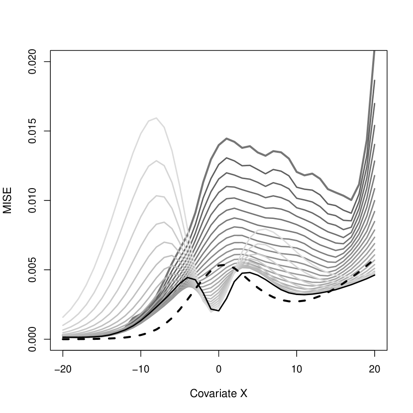
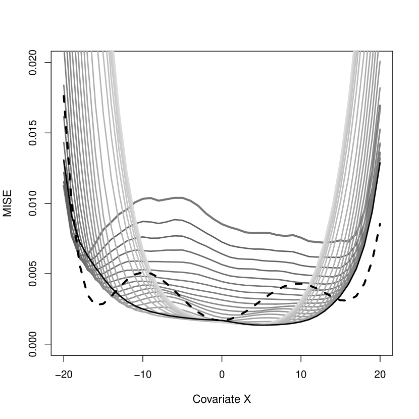
Figure 1: MISE of the proposed estimator $\widehat{S}_{h}^{c}(t|x)$ for a selection of $25$ bandwidths from the lowest (darkest grey line) to the highest (lightest grey line) in Scenario 1 (left) and Scenario 2 (right). Also shown are the MISE of $\widehat{S}_{h}(t|x)$ computed with the optimal bandwidth (solid black line), and of the estimator by ³ (dashed black line).

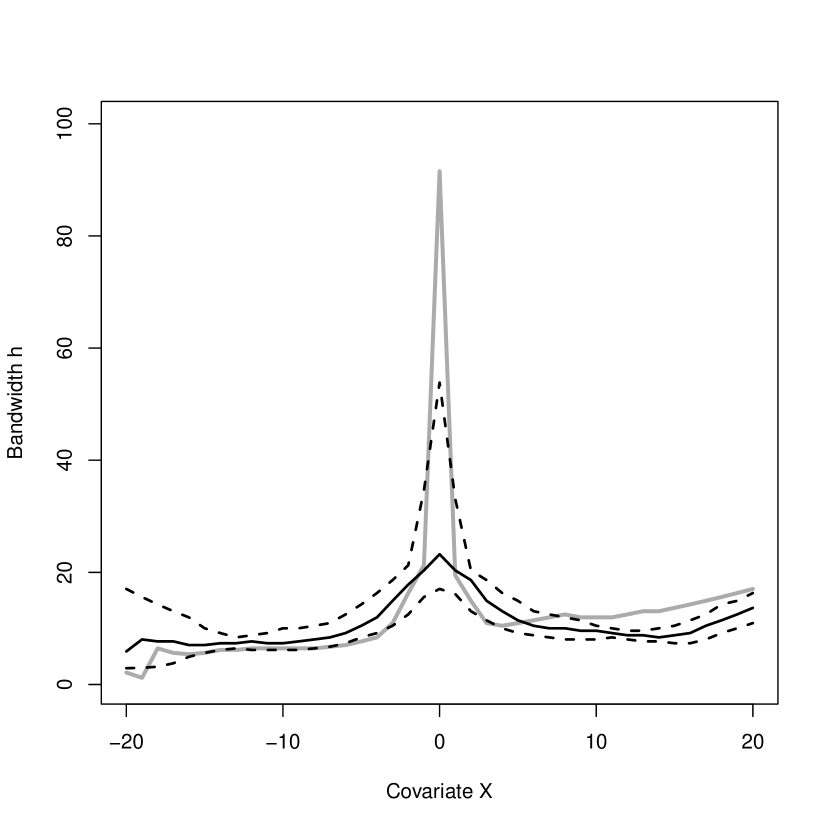
Figure 2: Median (solid black line) and first and third quartiles (dashed lines) of the bootstrap bandwidths for $\widehat{S}_{h}^{c}(t|x)$ in Scenario 1 (left) and Scenario 2 (right). The optimal bandwidth (solid grey line) is displayed as reference.

Table 1: Integrated squared bias ($\text{Ibias}{{}^{2}}$), integrated variance (Ivar) and MISE of the proposed estimator, $\widehat{S}_{h}^{c}(t|x)$, Beran’s estimator, $\widehat{S}_{h}(t|x)$, (both computed with the optimal bandwidth) and the semiparametric estimator by ³.

		Proposed					Beran					Semiparametric
Scenario	$x$	$h$	$\text{Ibias}{{}^{2}}$	Ivar	MISE		$h$	$\text{Ibias}{{}^{2}}$	Ivar	MISE		$\text{Ibias}{{}^{2}}$	Ivar	MISE
			$\times 10^{3}$	$\times 10^{3}$	$\times 10^{3}$			$\times 10^{3}$	$\times 10^{3}$	$\times 10^{3}$		$\times 10^{3}$	$\times 10^{3}$	$\times 10^{3}$
$1$	$-10$	$6.582$	$0.119$	$1.022$	$1.141$		$6.334$	$0.163$	$1.177$	$1.340$		$0.002$	$0.299$	$0.301$
	$0$	$20.000$	$0.371$	$1.834$	$2.205$		$20.000$	$0.119$	$1.927$	$2.046$		$0.035$	$5.280$	$5.315$
	$10$	$12.152$	$0.375$	$2.902$	$3.277$		$12.387$	$0.355$	$2.885$	$3.240$		$0.365$	$2.340$	$2.705$
$2$	$-10$	$25.874$	$0.076$	$2.206$	$2.282$		$23.492$	$0.065$	$2.501$	$2.566$		$3.962$	$1.122$	$5.084$
	$0$	$36.867$	$0.058$	$1.517$	$1.575$		$30.392$	$0.151$	$1.632$	$1.783$		$0.034$	$1.641$	$1.675$
	$10$	$26.721$	$0.103$	$1.474$	$1.577$		$28.497$	$0.058$	$1.492$	$1.550$		$1.026$	$3.282$	$4.308$

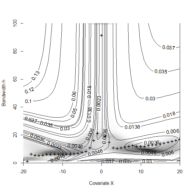
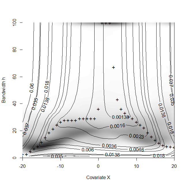
Figure 3: Contour plots of the MISE of $\widehat{S}_{h}^{c}(t|x)$ as a function of the bandwidth $h$ and the covariate value $x$ in Scenario 1 (left) and Scenario 2 (right). For each value of covariate, the optimal bandwidth is marked with a cross. The density of the bootstrap bandwidths is shown in grey scale.

Figure 4: MISE of $\widehat{S}_{h}^{c}(t|x)$ as a function of the bandwidth $h$ for four different values of the covariate $x=-10$ (solid line), $x=0$ (dotted), $x=5$ (dot-dashed) and $x=10$ (long dash) in Scenario 1 (left) and Scenario 2 (right). For each value of covariate, the optimal bandwidth where the minimum MISE is reached is marked with a cross.

The performance of the bootstrap bandwidth selector was assessed using $B=1000$ resamples. Figure 2 displays the quartiles of the selected bootstrap bandwidths together with the optimal bandwidth. Corresponding contour plots in Figure 3 show the density of the bootstrap bandwidths and the MISE of $\widehat{S}_{h}^{c}(t|x)$ as a function of the bandwidth $h$ and the covariate value $x$. Figure 4 shows the MISE of $\widehat{S}_{h}^{c}(t|x)$ as a function of the bandwidth $h$, for four values of the covariate. Figure 2 and Figure 3 illustrate that the bootstrap bandwidth approximates quite well the optimal bandwidth. Note that in Figure 3 vertical contour lines indicate that, given $x$, the MISE of $\widehat{S}_{h}^{c}(t|x)$ tends to be constant as a function of $h$. Therefore, different bandwidths would yield approximately the same MISE. In those cases, the bootstrap bandwidth being far from the optimal bandwidth does not imply a loss of efficiency. Similar results are observed in Figure 4. For example, let us consider $x=0$ in Scenario 2, we see that the MISE initially decreases as the bandwidth increases, although afterwards it becomes constant.

5 Application to real data

To illustrate the practical performance of $\widehat{S}_{h}^{c}(t|x)$ we considered a dataset of $233$ patients of sarcoma cancer aged $20-90$ years old from the University Hospital of Santiago de Compostela, Spain (CHUS). Sarcoma is a rare type of cancer that represents $1\%$ of all adult solid malignancies. If a tumor can be surgically removed to render the patient with sarcoma free of detectable disease, $5$ years is the survival time at which sarcoma oncologists assume long-term remissions ¹⁰. Overall, $59$ patients died from sarcoma, and the remaining $174$ patients were censored. Among censored patients, $18$ patients were tumor free for more than five years. Hence, they were assumed to be long-term survivors. The aim was to estimate the survival time of the patients until death from sarcoma as a function of covariates such as the age at diagnosis, sex, tumor site, cancer spread (metastasis) and the margin status. The variables selected for estimating the survival probabilities were previously reported to be related to long-term sarcoma survival ⁸, ¹² among others.

Table 2 shows the descriptive demographic and clinical characteristics of sarcoma patients by age, sex and relevant clinical factors. Of the $233$ patients, $100~{}(42.9\%)$ were males. Tumor site was categorized as retroperitoneal, extremities, or other. Most tumors were found in the retroperitoneum $(37\%)$ and in the extremities $(30\%)$, with other areas of the body accounting for about $33\%$. Fifty-five $(32.9\%)$ patients were diagnosed of metastatic sarcoma.

Figure 5 compares the results obtained by using the proposed estimator $\widehat{S}_{h}^{c}(t|x)$, which takes into account the 18 long-term survivors, with Beran’s estimator $\widehat{S}_{h}(t|x)$, which ignores individuals known to be cured and treats them as simply censored observations. Both estimators were computed with the corresponding bootstrap bandwidth. The semiparametric estimator of ³ was also considered as reference. All estimators show that the survival curve decreases when age increases from $40$ to $90$ years. We find the largest differences between the proposed estimator and Beran’s estimator at the right tail of the distribution, where the survival curve for $\widehat{S}^{c}_{h}(t|x)$ is slightly higher. Since the cure probability can be obtained as the limit of $S(t|x)$ when $t\rightarrow\infty$ using the proposed estimator of the survival curve will yield in higher estimates of the probability of cure.

On the other hand, the survival curve estimated by the semiparametric estimator of ³ tends to decrease much slower than those obtained with the nonparametric estimators $\widehat{S}^{c}_{h}(t|x)$ and $\widehat{S}_{h}(t|x)$, suggesting that further testing is required to provide evidence that assumptions in the semiparametric model are fulfilled.

Figure 5 on the right shows the survival curves of sarcoma patients stratified by the margin status. In this case, the proposed estimator in an unconditional setting $\widehat{S}_{n}^{c}(t)$ is applied and the ¹⁵ estimator is considered as reference. The survival curves tend to decrease with time in both subgroups. The positive margin survival curve decreases slightly faster than the negative survival curve. In addition, the distinction between $\widehat{S}_{n}^{c}(t)$ and the Kaplan-Meier estimator is found at the right tail of the distribution with the survival curves estimated by $\widehat{S}^{c}_{n}(t)$ being slightly higher than the Kaplan-Meir curves. For example, the survival probability, at the tail of the distribution, for patients with negative margins is around $0.51$ when estimated by $\widehat{S}_{n}^{c}(t)$, while it is around $0.47$ when estimated by the Kaplan-Meier estimator. Again, the estimated probability of cure is slightly higher when the survival curve is fitted taking into account the known cured subjects.

Table 2: Descriptive demographic and clinical characteristics of sarcoma patients stratified by age, sex, location of the sarcoma, metastatic and the margin status. In addition, the total number of patients for each subgroup ($n$), the number of patients died of sarcoma (death), those who were known to be cured (cured) and those with unknown cure status (unknown) are given.

Characteristics	$n$ ($\%$)		Death		Censored
					Cured	Unknown
Age†
$<60$	$105~{}(45.3\%)$		$25$		$9$	$71$
$\geq 60$	$127~{}(54.7\%)$		$33$		$9$	$85$
Sex
Male	$100~{}(42.9\%)$		$25$		$7$	$68$
Female	$133~{}(57.1\%)$		$34$		$11$	$88$
Tumor site†
Retroperitoneal	$86~{}(37.2\%)$		$28$		$4$	$54$
Extremities	$70~{}(30.3\%)$		$14$		$5$	$51$
Other sites	$75~{}(32.5\%)$		$16$		$9$	$50$
Metastatic†
No	$112~{}(67.1\%)$		$11$		$9$	$92$
Yes	$55~{}(32.9\%)$		$32$		$3$	$20$
Margin status†
Negative	$133~{}(65.8\%)$		$25$		$12$	$95$
Positive	$69~{}(34.2\%)$		$17$		$3$	$49$
† Contains a few missing data.

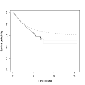
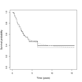
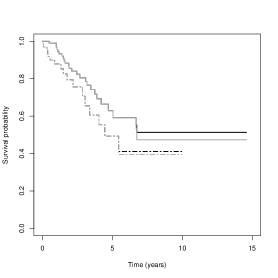
Figure 5: Survival estimates for sarcoma patients aged 40 (left) and 90 (center) years are obtained with the proposed estimator $\widehat{S}^{c}_{h}(t|x)$ (solid black line) and Beran’s estimator $\widehat{S}_{h}(t|x)$ (solid grey line), both computed with the corresponding bootstrap bandwidth, and the semiparametric estimator of ³ (dashed grey line). The right figure shows survival estimates stratified by the margin status, negative margin (solid lines) versus positive margin (dashed lines). These estimates are computed using the proposed estimator $\widehat{S}_{n}^{c}(t)$ (black lines) and the Kaplan-Meier estimator (grey lines).

6 Discussion

The proposed nonparametric estimator of the survival function takes advantage of the additional cure status information that Beran’s estimator ignores. As a further step, it could be used to derive nonparametric estimators for the cure probability and the latency function.

Thus far, the estimation procedure was discussed involving a single continuous covariate. It would be of interest to extend our estimator to the case of multiple covariates, with $\mathbf{X}$ a vector of mixed discrete, categorical and/or continuous variables. One possibility is to consider product kernels (Li and Racine,, 2008). Another possibility is to use dimension reduction techniques like a single-index model. Specifically, the idea is to apply the proposed estimator of the survival function with a new covariate given by an estimator of the index $\widetilde{\mathbf{X}}=\mathbf{\beta}^{T}\mathbf{X}$, with $\mathbf{\beta}$ a parameter vector of the same dimension of $\mathbf{X}$. Semiparametric index estimation of the conditional distribution in the presence of right censoring was considered recently by ²⁰.

Although the proposed estimator utilizes the cure status information and shows good results both theoretically and practically, it is not without limitations. It is competitive over Beran’s estimator in terms of the MISE, showing a general better behavior. But for some values of the covariate it does not result in an improvement but a slightly worse MISE performance. The clear gain in terms of the integrated variance could be cancelled out by the integrated squared bias, which depends on the cure probability, the conditional censoring distribution and the conditional probability of observed cured individuals. For the semiparametric estimator by ³, our numerical experience indicates that if the sample size is small (less than 100), it is challenging to obtain stable values for the model parameters.

The R package npcure by ²⁴ provides the nonparametric estimation and testing procedures in mixture cure models proposed by López-Cheda et al., 2017a , , 2020, including the Beran’s estimator. The situation when cure status is partially known is not currently supported by the package but will be considered in future versions. Further, the estimator of the conditional survival function introduced in this paper and subsequent estimators of the cure rate and latency functions will be incorporated in the upgraded package.

Conflict of interest

The authors have declared no conflicts of interest.

ORCID

Wende Clarence Safari * | https://orcid.org/0000-0003-4639-7552
Ignacio López-de-Ullibarri * | https://orcid.org/0000-0002-3438-6621
M. Amalia Jácome * | https://orcid.org/0000-0001-7000-9623

SUPPORTING INFORMATION

Supplementary Material includes the proofs of Theorem 2.3–2.4 and Lemmas 1–5 which are needed for deducing the asymptotic bias and variance of $\widehat{S}_{h}^{c}(t|x)$. It also includes: the simulation results for sample sizes $n=50$, $100$, $200$, and proportions of observed cured data $\pi=0.2,0.8$, $1$; and additional simulations to study the effect of the pilot bandwidth on the estimates. Additional supporting information including source code to reproduce the results can be found online in the Supporting Information section at the end of the article. The following assumptions are made.

• Let $I=\left[x_{1},x_{2}\right]$ be an interval contained in the support of the density function of $X$, $m(x)$, such that

  $$0<\gamma=\inf_{x\in I_{\varepsilon}}m(x)<\sup_{x\in I_{\varepsilon}}m(x)=\Gamma<\infty$$

  for some $I_{\varepsilon}=[x_{1}-\varepsilon,x_{2}+\varepsilon]$ with $\varepsilon>0$ and $0<\varepsilon\Gamma<1$. And for all $x\in I$, $Y$, $C$ are conditionally independent at $X=x$.

• There exist $a,b\in\mathbb{R}$, with $a<b$ satisfying $J\left(t|x\right)\geq\theta>0\text{ \ for \ }(t,x)\in[a,b]\times I_{\varepsilon}.$

The first derivative with respect to $x$ of function $m(x)$ exists and is continuous in $x\in I_{\varepsilon}$, and the first derivatives with respect to $x$ of functions $H(t|x)$, $H^{1}(t|x)$ and $H^{11}(t|x)$ exist and are continuous and bounded in $(t,x)\in[0,\infty)\times I_{\varepsilon}$. The second derivative with respect to $x$ of function $m(x)$ exists and is continuous in $x\in I_{\varepsilon}$, and the second derivatives with respect to $x$ of functions $H(t|x)$, $H^{1}(t|x)$ and $H^{11}(t|x)$ exist and are continuous and bounded in $(t,x)\in[0,\infty)\times I_{\varepsilon}$. The first derivatives with respect to $t$ of $H(t|x)$, $H^{1}(t|x)$ and $H^{11}(t|x)$ exist and are continuous in $\left(t,x\right)\in[a,b]\times I_{\varepsilon}$. The second derivatives with respect to $t$ of $H(t|x)$, $H^{1}(t|x)$ and $H^{11}(t|x)$ exist and are continuous in $\left(t,x\right)\in[a,b]\times I_{\varepsilon}$. The first derivative with respect to $x$ and the second derivative with respect to $t$ of $H(t|x)$, $H^{1}(t|x)$ and $H^{11}(t|x)$ exist and are continuous in $(t,x)\in[a,b]\times I_{\varepsilon}$. The (sub)densities corresponding to the (sub)distribution functions $H(t|x)$, $H^{1}(t|x)$ and $H^{11}(t|x)$ are bounded away from $0$ in $[a,b]\times I_{\varepsilon}$. The kernel function $K(v)$ is a symmetrical density with zero mean, vanishing outside $(-1,1)$, and the total variation is less than $\lambda<\infty$. Motivation of the proposed estimators. The cumulative hazard function $\Lambda(t|x)$ can be written as follows:

$$\Lambda(t\mid x)= \int_{0}^{t}\dfrac{dF\left(v\mid x\right)}{1-F\left(v^{-}\mid x\right)}=\int_{0}^{t}\dfrac{\left\{1-G(v^{-}\mid x)+G^{11}(v^{-}\mid x)\right\}dF(v\mid x)}{\left\{1-G(v^{-}\mid x)+G^{11}(v^{-}\mid x)\right\}\{1-F(v^{-}\mid x)\}},$$ (A1)

where $G^{11}(t|x)=P\left(C\leq t,\xi=1,\nu=1|X=x\right)$ is the conditional censoring subdistribution of the individuals observed to be cured. The numerator in (A1) is $dH^{1}(t\mid x)$:

$$\int_{0}^{t}\left\{1-G(v^{-}\mid x)+G^{11}(v^{-}\mid x)\right\}dF(v\mid x)$$

$$=\int_{0}^{t}P(C\geq v\mid X=x)dF(v\mid x)+\int_{0}^{t}P(C<v,\xi=1,\nu=1\mid X=x)dF(v\mid x)$$

$$=P(Y\leq t,C\geq Y\mid X=x)+P(Y\leq t,C<Y,\xi=1,Y=\infty\mid X=x)$$

$$=P(T\leq t,\delta=1\mid X=x)=H^{1}(t\mid x).$$ (A2)

Similarly, the denominator in (A1) is $J(t^{-}|x)$:

$$\left\{1-G(t^{-}\mid x)+G^{11}(t^{-}\mid x)\right\}\{1-F(t^{-}\mid x)\}$$

$$=\{P(C\geq t\mid X=x)+P(C<t,\xi=1,\nu=1\mid X=x)\}P(Y\geq t\mid X=x)$$

$$=P(Y\geq t,C\geq t\mid X=x)+P(Y\geq t,C<t,\xi=1,\nu=1\mid X=x)$$

$$=P(T\geq t\mid X=x)+P(T<t,\xi=1,\nu=1\mid X=x)$$

$$=1-H\left(t^{-}\mid x\right)+H^{11}\left(t^{-}\mid x\right)=J(t^{-}\mid x).$$ (A3)

Taking (A2) and (A3) into account, (A1) can be written as

$$\Lambda(t\mid x)=\int_{0}^{t}\dfrac{dH^{1}(v\mid x)}{J(v^{-}\mid x)}.$$ (A4)

Consider the Nadaraya-Watson kernel estimates of $H^{1}(t|x)$ and $J(t^{-}|x)$:

$$\widehat{H}_{h}^{1}(t\mid x) =\sum_{i=1}^{n}B_{hi}(x)\textbf{1}\left(T_{i}\leq t,\delta_{i}=1\right),$$ (A5)

$$\widehat{J}_{h}(t^{-}\mid x) =\sum_{i=1}^{n}B_{hi}(x)\textbf{1}\left(T_{i}\geq t\right)+\sum_{i=1}^{n}B_{hi}(x)\textbf{1}\left(T_{i}<t,\xi_{i}\nu_{i}=1\right).$$ (A6)

The estimator of $\Lambda(t|x)$ when the cure status is partially known, $\widehat{\Lambda}^{c}_{h}(t|x)$, is obtained by plugging in (A4) the estimates (A5) and (A6). As for the estimator of the survival function, it can be shown that $S(t|x)=\exp\left\{-\Lambda(t|x)\right\}$. By considering a Taylor’s expansion of the exponential function around 0 and evaluating it at each increment of $\widehat{\Lambda}_{h}^{c}(t|x)$, the estimator $\widehat{S}^{c}_{h}(t|x)$ in (3) is obtained.

Proof of Proposition 2.1. The estimator $\widehat{S}_{h}^{c}(t|x)$ has the following properties

1. If there is no known cure status, $\widehat{S}_{h}^{c}(t|x)$ reduces to $\widehat{S}_{h}(t|x)$.

   Proof .1.

   It is straightforward since $\xi_{i}\nu_{i}=0$, $i=1,\ldots,n$.

2. In the specific case when some individuals are observed as cured when their survival time exceeds a known fixed cure threshold, $\widehat{S}_{h}^{c}(t|x)$ reduces to $\widehat{S}_{h}(t|x)$.

   Proof .2.

   Assume there exists a common specific known cure threshold $d_{i}=d$ for $i=1,\ldots,n$. This implies that in the ordered sample, $\left\{\left(X_{\left[i\right]},T_{\left(i\right)},\delta_{\left[i\right]},\xi_{\left[i\right]},\xi_{\left[i\right]}\nu_{\left[i\right]}\right):i=1,\ldots,n\right\}$, the $n_{1}$ first observations correspond to individuals with $T_{\left(i\right)}<d$ either not cured or with unknown cure status ($\xi_{[i]}\nu_{[i]}=0$), and the remaining $m$ observations are cured individuals with $T_{\left(i\right)}\geq d$ and $\xi_{[i]}\nu_{[i]}=1$. Therefore,

   $$\widehat{S}_{h}^{c}\left(t\mid x\right)=\prod_{i=1}^{n}\left\{1-\frac{\delta_{\left[i\right]}B_{h\left[i\right]}\left(x\right)\textbf{ 1}\left(T_{(i)}\leq t\right)}{\sum_{j=i}^{n_{1}}B_{h\left[j\right]}\left(x\right)+\sum_{j=n_{1}+1}^{n}B_{h\left[j\right]}\left(x\right)}\right\}=\prod_{i=1}^{n}\left\{1-\frac{\delta_{\left[i\right]}B_{h\left[i\right]}\left(x\right)\textbf{1}\left(T_{(i)}\leq t\right)}{\sum_{j=i}^{n}B_{h\left[j\right]}\left(x\right)}\right\}=\widehat{S}_{h}(t\mid x)$$

   This completes the proof.

3. When there is no censoring, the estimator $\widehat{S}_{h}^{c}(t|x)$ reduces to the kernel type estimator of the conditional survival function.

   Proof .3.

   Without censoring, $T_{i}=Y_{i},\delta_{i}=1$ and the cure status is always observed $\xi_{i}=1$. In this situation, the $n=n_{1}+m$ observations can be ordered and split into the $n_{1}$ uncured individuals with finite lifetimes $Y_{i}$, and the $m$ cured individuals with lifetime $Y_{i}=\infty$. Thus,

   $$\widehat{S}_{h}^{c}(t\mid x)= \prod_{i=1}^{n}\left\{1-\frac{B_{h[i]}\left(x\right)\textbf{1}\left(Y_{\left(i\right)}\leq t\right)}{\sum_{j=i}^{n}B_{h[j]}\left(x\right)+\sum_{j=1}^{i-1}B_{h[j]}\left(x\right)\textbf{1}\left(\nu_{[j]}=1\right)}\right\}$$

   $$= \prod_{i=1}^{n}\left\{1-\frac{B_{h[i]}\left(x\right)\textbf{1}\left(Y_{\left(i\right)}\leq t\right)}{\sum_{j=i}^{n_{1}}B_{h[j]}\left(x\right)+\sum_{j=n_{1}+1}^{n}B_{h[j]}\left(x\right)}\right\}=\prod_{i:Y_{\left(i\right)}\leq t}\left\{\frac{\sum_{j=i+1}^{n}B_{h[j]}\left(x\right)}{\sum_{j=i}^{n}B_{h[j]}\left(x\right)}\right\}.$$

   Note that the kernel estimator of the survival function $\widetilde{S}_{h}(t|x)=\sum_{i=1}^{n}B_{h[i]}\left(x\right)\textbf{1}(Y_{(i)}>t)$ is a step function with jumps $B_{hi}\left(x\right)$ at the observations, $Y_{i}$. By defining $k=\max\{i:Y_{\left(i\right)}\leq t\}$ i.e., $Y_{\left(k\right)}\leq t$ and $Y_{\left(k+1\right)}>t$, one can write

   $$\prod_{i:Y_{\left(i\right)}\leq t}\left\{\frac{\sum_{j=i+1}^{n}B_{h[j]}\left(x\right)}{\sum_{j=i}^{n}B_{h[j]}\left(x\right)}\right\} =\prod_{i:Y_{\left(i\right)}\leq t}\left\{\frac{\widetilde{S}_{h}(Y_{(i)}\mid x)}{\widetilde{S}_{h}(Y_{(i-1)}\mid x)}\right\}=\frac{\widetilde{S}_{h}(Y_{\left(1\right)}\mid x)}{1}\ \frac{\widetilde{S}_{h}(Y_{\left(2\right)}|x)}{\widetilde{S}_{h}(Y_{\left(1\right)}\mid x)}\ \ldots\ \frac{\widetilde{S}_{h}(Y_{\left(k\right)}\mid x)}{\widetilde{S}_{h}(Y_{\left(k-1\right)}\mid x)}$$

   $$=\widetilde{S}_{h}(Y_{\left(k\right)}\mid x)=\sum_{i=1}^{n}B_{h[i]}\left(x\right)\textbf{1}(Y_{(i)}>t).$$

   This completes the proof.

4. In an unconditional setting the proposed estimator is

   $$\widehat{S}_{n}^{c}\left(t\right)=\prod_{i=1}^{n}\left\{1-\frac{\delta_{[i]}\textbf{1}\left(T_{\left(i\right)}\leq t\right)}{n-i+1+\sum_{j=1}^{i-1}\textbf{1}\left(\xi_{[j]}\nu_{[j]}=1\right)}\right\}.$$

   Proof .4.

   In unconditional setting the weights are $1/n$ for $i=1,\ldots,n$. Thus, the proposed estimator becomes

   $$\widehat{S}_{n}^{c}\left(t\right)=\prod_{i=1}^{n}\left\{1-\frac{\delta_{[i]}\frac{1}{n}\textbf{1}\left(T_{\left(i\right)}\leq t\right)}{\frac{1}{n}(n-i+1)+\frac{1}{n}\sum_{j=1}^{i-1}\textbf{1}\left(\xi_{[j]}\nu_{[j]}=1\right)}\right\}.$$

   In the particular case where an individual is known to be cured only if the observed time is greater than a known fixed time, say $d$, with $n=n_{1}+m$ observations, when $m$ are identified as cured, the ordered observed lifetimes are $T_{(1)}\leq\ldots\leq T_{(n_{1})}$ strictly lower than $d$, and the $m$ cured individuals with $T_{(i)}\geq d$. Thus, $\widehat{S}_{h}^{c}(t|x)$ reduces to the generalized maximum likelihood estimator in ¹⁶:

   $$\widehat{S}_{n}^{c}(t) =\prod_{i=1}^{n}\left\{1-\frac{\delta_{[i]}\frac{1}{n}\textbf{1}\left(T_{\left(i\right)}\leq t\right)}{\frac{1}{n}(n_{1}-i+1)+\frac{1}{n}m}\right\}=\prod_{i=1}^{n}\left\{1-\frac{\delta_{[i]}\textbf{1}(T_{(i)}\leq t)}{n-i+1}\right\}.$$

   This completes the proof.

Proof of Proposition 2.2. The proof follows the argument in Theorem 2 in ²¹ and Theorem 1 in ¹⁶. To derive the expression of the local likelihood of the mixture cure model, we consider the three potential cases for the $i$th observation:

Case 1: $\delta_{i}=1$.

The event is observed and the individual is not cured. We observe $Y_{i}=t_{i},\nu_{i}=0$, with probability:

$$P\left(Y_{i}=t_{i},C_{i}>t_{i},\nu_{i}=0\mid X=x\right)= P\left(C_{i}>t_{i}\mid Y_{i}=t_{i},\nu_{i}=0,X=x\right)$$

$$\times P\left(Y_{i}=t_{i}\mid\nu_{i}=0,X=x\right)P\left(\nu_{i}=0\mid X=x\right)$$

$$= S_{C\mid Y,X,\nu=0}\left(t_{i}\mid x\right)\left\{S_{0}(t_{i}^{-}\mid x)-S_{0}(t_{i}\mid x)\right\}p\left(x\right),$$

where $S_{C\mid Y,X,\nu=0}(t\mid x)$ is the conditional survival function for the censoring variable $C$ for uncured individuals.

Case 2: $(\delta_{i}=0,\xi_{i}\nu_{i}=0)$.

The individual is censored and the cure status is unknown. We observe $C_{i}=t_{i}$, and $\nu_{i}$ is unknown, with probability:

$$P\left(Y_{i}>t_{i},C_{i}=t_{i}\mid X=x\right)= P\left(Y_{i}>t_{i},C_{i}=t_{i},\nu_{i}=1\mid X=x\right)P(\nu_{i}=1\mid X=x)$$

$$+P\left(Y_{i}>t_{i},C_{i}=t_{i},\nu_{i}=0\mid X=x\right)P(\nu_{i}=0\mid X=x)$$

$$= f_{C\mid Y,X,\nu=1}\left(t_{i}\mid x\right)\left\{1-p\left(x\right)\right\}+f_{C\mid Y,X,\nu=0}\left(t_{i}\mid x\right)\times S_{0}\left(t_{i}\mid x\right)p\left(x\right),$$

where $f_{C\mid Y,X,\nu=1}(t\mid x)$ and $f_{C\mid Y,X,\nu=0}(t\mid x)$ are the conditional density functions for the censoring variable $C$ of the cured and uncured individuals, respectively.

Case 3: $\left(\delta_{i}=0,\xi_{i}\nu_{i}=1\right)$.

The individual is censored and known to be cured. We observe $C_{i}=t_{i},\nu_{i}=1$, with probability

$$P\left(Y_{i}>t_{i},C_{i}=t_{i},\nu_{i}=1\mid X=x\right)= P\left(C_{i}=t_{i}\mid Y_{i}>t_{i},\nu_{i}=1,X=x\right)$$

$$\times P\left(Y_{i}>t_{i}\mid\nu_{i}=1,X=x\right)P\left(\nu_{i}=1\mid X=x\right)$$

$$= f_{C\mid Y,X,\nu=1}\left(t_{i}\mid x\right)\left\{1-p\left(x\right)\right\}.$$

In the absence of specification of the distribution of $X$, the terms in the log-likelihood are weighted with the kernel weights $B_{h[i]}(x)$. Then, the local likelihood of the data is

$$L\left(X,T,\delta,\xi,\nu\right)= \prod\limits_{i=1}^{n}\left[S_{C\mid Y,X,\nu=0}\left(T_{\left(i\right)}\mid x\right)\left\{S_{0}(T_{\left(i\right)}^{-}\mid x)-S_{0}(T_{\left(i\right)}\mid x)\right\}p\left(x\right)\right]^{B_{h\left[i\right]}\left(x\right)\bm{1}\left(\delta_{\left[i\right]}=1\right)}$$

$$\times\left[f_{C\mid Y,X,\nu=1}\left(T_{\left(i\right)}\mid x\right)\left\{1-p\left(x\right)\right\}+f_{C\mid Y,X,\nu=0}\left(T_{\left(i\right)}\mid x\right)S_{0}\left(T_{\left(i\right)}\mid x\right)p\left(x\right)\right]^{B_{h\left[i\right]}\left(x\right)\bm{1}\left(\delta_{\left[i\right]}=0,\xi_{\left[i\right]}\nu_{\left[i\right]}=0\right)}$$

$$\times\left[f_{C\mid Y,X,\nu=1}\left(T_{\left(i\right)}\mid x\right)\left\{1-p\left(x\right)\right\}\right]^{B_{h\left[i\right]}\left(x\right)\bm{1}\left(\delta_{\left[i\right]}=0,\xi_{[i]}\nu_{[i]}=1\right)}.$$

If the distribution of the censoring variable $C$ is conditionally independent of $Y$ and the cure status $\nu$ given the covariate $X$, then

$$L\left(X,T,\delta,\xi,\nu\right)= \prod\limits_{i=1}^{n}\left[q_{i}(x)p\left(x\right)\right]^{B_{h\left[i\right]}\left(x\right)\textbf{1}\left(\delta_{\left[i\right]}=1\right)}\times\left\{1-p\left(x\right)+S_{0}\left(T_{\left(i\right)}\mid x\right)p\left(x\right)\right\}^{B_{h\left[i\right]}\left(x\right)\textbf{1}\left(\delta_{\left[i\right]}=0,\xi_{\left[i\right]}\nu_{\left[i\right]}=0\right)}$$

$$\times\left\{1-p\left(x\right)\right\}^{B_{h\left[i\right]}\left(x\right)\textbf{1}\left(\delta_{\left[i\right]}=0,\xi_{[i]}\nu_{[i]}=1\right)}\times\left(1-\sum_{j=1}^{i-1}g_{j}\left(x\right)\right)^{B_{h\left[i\right]}\left(x\right)\textbf{1}\left(\delta_{\left[i\right]}=1\right)}g_{i}\left(x\right)^{B_{h\left[i\right]}\left(x\right)\textbf{1}\left(\delta_{\left[i\right]}=0\right)},$$ (A7)

where, for $i=1,\ldots,n$, $q_{i}\left(x\right)=S_{0}(T_{(i)}^{-}|x)-S_{0}(T_{(i)}|x)$ are the increments of $S_{0}\left(t|x\right)$, and $g_{i}\left(x\right)=G(T_{(i)}|x)-G(T_{(i)}^{-}|x)$ the increments of $G\left(t|x\right)$. Let $P_{i}\left(x\right)=p\left(x\right)q_{i}\left(x\right)$ be the increments of $S\left(t|x\right)$, then $\sum_{i=1}^{n}P_{i}\left(x\right)=p\left(x\right)$. Maximizing (A7) is equivalent to maximizing the likelihood

$$L\left(X,T,\delta,\xi,\nu\right)= \prod\limits_{i=1}^{n}P_{i}\left(x\right)^{B_{h\left[i\right]}\left(x\right)\textbf{1}\left(\delta_{\left[i\right]}=1\right)}\left(1-\sum_{j=1}^{i-1}P_{j}\left(x\right)\right)^{B_{h\left[i\right]}\left(x\right)\textbf{1}\left(\delta_{[i]}=0,\xi_{[i]}\nu_{[i]}=0\right)}\times\left(1-\sum_{j=1}^{n}P_{j}\left(x\right)\right)^{B_{h\left[i\right]}\left(x\right)\textbf{1}\left(\delta_{\left[i\right]}=0,\xi_{[i]}\nu_{[i]}=1\right)}.$$ (A8)

Further, consider the functions $\lambda_{i}\left(x\right)=P_{i}\left(x\right)/\left\{1-\sum_{j=1}^{i-1}P_{j}\left(x\right)\right\}$ satisfying

$$1-\sum_{j=1}^{k}P_{j}\left(x\right)=\prod_{j=1}^{k}\{1-\lambda_{j}\left(x\right)\}.$$ (A9)

Then, the increments $P_{i}\left(x\right)$ can be written in terms of $\lambda_{i}\left(x\right)$:

$$P_{i}\left(x\right)=\lambda_{i}\left(x\right)\left\{1-\sum_{j=1}^{i-1}P_{j}\left(x\right)\right\}=\lambda_{i}\left(x\right)\prod_{j=1}^{i-1}\left\{1-\lambda_{j}\left(x\right)\right\}.$$ (A10)

By substituting (A9) and (A10) in (A8), the likelihood (A8) is

$$L\left(X,T,\delta,\xi,\nu;p,S_{0}\right)= \prod\limits_{i=1}^{n}\lambda_{i}\left(x\right)^{B_{h\left[i\right]}\left(x\right)\bm{1}\left(\delta_{\left[i\right]}=1\right)}\prod_{i=1}^{n}\left[\prod_{j=1}^{i-1}\left\{1-\lambda_{j}\left(x\right)\right\}\right]^{B_{h\left[i\right]}\left(x\right)\bm{1}\left(\delta_{\left[i\right]}=1\right)}$$

$$\times\prod_{i=1}^{n}\left[\prod_{j=1}^{i-1}\left\{1-\lambda_{j}\left(x\right)\right\}\right]^{B_{h\left[i\right]}\left(x\right)\bm{1}\left(\delta_{\left[i\right]}=0,\xi_{\left[i\right]}\nu_{\left[i\right]}=0\right)}\times\prod\limits_{i=1}^{n}\left[\prod_{j=1}^{n}\left\{1-\lambda_{j}\left(x\right)\right\}\right]^{B_{h\left[i\right]}\left(x\right)\bm{1}\left(\delta_{\left[i\right]}=0,\xi_{[i]}\nu_{[i]}=1\right)}.$$

Taking into account that $\prod_{i=1}^{n}\left[\prod_{j=1}^{i-1}a_{j}\right]^{b_{i}}=\prod_{i=1}^{n}a_{i}^{\sum_{j=i+1}^{n}b_{j}}$, where $a_{i}$ and $b_{i}$, $i=1,\ldots,n$, are arbitrary sequences of nonnegative numbers, the likelihood becomes

$$L\left(X,T,\delta,\xi,\nu;p,S_{0}\right)= \prod_{i=1}^{n}\lambda_{i}\left(x\right)^{B_{h\left[i\right]}\left(x\right)\bm{1}\left(\delta_{\left[i\right]}=1\right)}\times\prod_{i=1}^{n}\left\{1-\lambda_{i}\left(x\right)\right\}^{\sum_{j=i+1}^{n}B_{h\left[j\right]}\left(x\right)\bm{1}\left(\xi_{\left[j\right]}\nu_{\left[j\right]}=0\right)+\sum_{j=1}^{n}B_{h\left[j\right]}\left(x\right)\bm{1}\left(\delta_{[j]}=0,\xi_{[j]}\nu_{[j]}=1\right)}.$$

Maximizing the likelihood $L\left(X,T,\delta,\xi,\nu;p,S_{0}\right)$ is equivalent to maximizing the local log-likelihood:

$$\Psi\{\lambda_{1}\left(x\right),\dots,\lambda_{n}\left(x\right)\}= \sum_{i=1}^{n}\left[B_{h\left[i\right]}\left(x\right)\bm{1}\left(\delta_{\left[i\right]}=1\right)\log\lambda_{i}\left(x\right)\right.$$

$$\left.+\left\{\sum_{j=i+1}^{n}B_{h\left[j\right]}\left(x\right)\bm{1}\left(\xi_{\left[j\right]}\nu_{\left[j\right]}=0\right)+\sum_{j=1}^{n}B_{h\left[j\right]}\left(x\right)\bm{1}\left(\delta_{[j]}=0,\xi_{[j]}\nu_{[j]}=1\right)\right\}\log\left(1-\lambda_{i}\right)\right]$$

subject to $\prod_{i=1}^{n}\{1-\lambda_{i}\left(x\right)\}=1-p\left(x\right)$. The maximizer $\lambda_{i}\left(x\right)$ of the log-likelihood is

$$\widehat{\lambda}_{i}\left(x\right)= \frac{B_{h\left[i\right]}\left(x\right)\bm{1}\left(\delta_{\left[i\right]}=1\right)}{\sum_{j=i}^{n}B_{h\left[j\right]}\left(x\right)+\sum_{j=1}^{i-1}B_{h\left[j\right]}\left(x\right)\bm{1}\left(\xi_{[j]}\nu_{[j]}=1\right)}.$$

In virtue of (A10), the estimator $\widehat{S}_{h}^{c}(t|x)$ computed by forming the product of $\widehat{\lambda}_{i}$’s such that $T_{(i)}\leq t$ is the nonparametric maximum likelihood estimator of $S(t|x)$. This completes the proof of Proposition 2.2.

Proof of Corollary 2.5. The dominant part of $\widehat{\Lambda}_{h}^{c}(t|x)-\Lambda(t|x)$ in Theorem 2.3 verifies

$$\sum_{i=1}^{n}B_{hi}(x)\zeta\left(T_{i},\delta_{i},\xi_{i},\nu_{i},t,x\right)= \int_{0}^{t}\frac{d\widehat{H}_{h}^{1}\left(v\mid x\right)}{J\left(v^{-}\mid x\right)}-\int_{0}^{t}\frac{\widehat{J}_{h}\left(v^{-}\mid x\right)}{J^{2}\left(v^{-}\mid x\right)}dH^{1}\left(v\mid x\right)$$

$$= \int_{0}^{t}\frac{d\widehat{H}_{h}^{1}\left(v\mid x\right)-dH^{1}(v\mid x)}{J\left(v^{-}\mid x\right)}-\int_{0}^{t}\frac{\widehat{J}_{h}\left(v^{-}\mid x\right)-J(v^{-}\mid x)}{J^{2}\left(v^{-}\mid x\right)}dH^{1}\left(v\mid x\right)$$

$$= \left[\frac{\widehat{H}_{h}^{1}\left(v\mid x\right)-H^{1}\left(v\mid x\right)}{J\left(v^{-}\mid x\right)}\right]_{0}^{t}+\int_{0}^{t}\frac{\widehat{H}_{h}^{1}\left(v\mid x\right)-H^{1}\left(v\mid x\right)}{J^{2}\left(v^{-}\mid x\right)}dJ(v\mid x)$$

$$-\int_{0}^{t}\frac{\widehat{J}_{h}\left(v^{-}\mid x\right)-J(v^{-}\mid x)}{J^{2}\left(v^{-}\mid x\right)}dH^{1}\left(v\mid x\right)$$

$$\leq \frac{1}{\theta}\sup_{a\leq t\leq b,x\in I}\mid\widehat{H}_{h}^{1}\left(t\mid x\right)-H^{1}\left(t\mid x\right)\mid+\frac{1}{\theta}\sup_{a\leq t\leq b,x\in I}\mid\widehat{H}_{h}^{1}\left(t\mid x\right)-H^{1}\left(t\mid x\right)\mid$$

$$-\frac{1}{\theta^{2}}\sup_{a\leq t\leq b,x\in I}\mid\widehat{J}_{h}\left(t\mid x\right)-J\left(t\mid x\right)\mid.$$

The last three terms in the inequality are bounded by applying Lemma 5 in ¹⁴, which holds not only for conditional survival functions like $1-H(t|x)$, but also for conditional subdistribution functions as $H^{1}(t|x)$ and $H^{11}(t|x)$ (see Remark 2 in ¹⁴ and the proof of Theorem 2.1 in ¹¹). As a consequence, the dominant term of $\widehat{\Lambda}_{h}^{c}(t|x)-\Lambda(t|x)$ is bounded by

$$\sup_{a\leq t\leq b,x\in I}\mid\sum\limits_{i=1}^{n}B_{hi}(x)\zeta\left(T_{i},\delta_{i},\xi_{i},\nu_{i},t,x\right)\mid=O\left\{\left(nh\right)^{-1/2}\left(\log n\right)^{1/2}\right\}.$$

Using the results of Theorem 2.4 it is straightforward to prove the second part of this corollary.

Proof of Proposition 2.6. From Theorem 2.4, the bias of the nonparametric estimator $1-\widehat{F}^{c}_{h}\left(t|x\right)$ is asymptotically equal to the expected value

$$\frac{(nh)^{-1}\left\{1-F\left(t\mid x\right)\right\}}{m\left(x\right)}\sum\limits_{i=1}^{n}K\left(\frac{x-X_{i}}{h}\right)\zeta\left(T_{i},\delta_{i},\xi_{i},\nu_{i},t,x\right)=I+II$$ (A11)

where

$$I= \frac{(nh)^{-1}\left\{1-F\left(t\mid x\right)\right\}}{m\left(x\right)}\Bigg{[}\sum\limits_{i=1}^{n}K\left(\frac{x-X_{i}}{h}\right)\zeta\left(T_{i},\delta_{i},\xi_{i},\nu_{i},t,x\right)-\text{E}\left\{\sum_{i=1}^{n}K\left(\frac{x-X_{i}}{h}\right)\zeta\left(T_{i},\delta_{i},\xi_{i},\nu_{i},t,x\right)\right\}\Bigg{]},$$ (A12)

$$II= \frac{(nh)^{-1}\{1-F\left(t\mid x\right)\}}{m\left(x\right)}\text{E}\left\{\sum\limits_{i=1}^{n}K\left(\frac{x-X_{i}}{h}\right)\zeta\left(T_{i},\delta_{i},\xi_{i},\nu_{i},t,x\right)\right\}.$$ (A13)

Since $E(I)=0$, the asymptotic bias of the estimator $1-\widehat{F}_{h}^{c}\left(t\mid x\right)$ is $II$. Using Lemmas 1 and 2 in the Supplementary Material,

$$II =\frac{h^{2}\left\{1-F\left(t\mid x\right)\right\}(\Phi_{c}^{\prime\prime}\left(x,t,x\right)m\left(x\right)+2\Phi_{c}^{\prime}\left(x,t,x\right)m^{\prime}\left(x\right))d_{K}}{2m\left(x\right)}+O\left(h^{4}\right),$$

with $\Phi_{c}^{\prime}(y,t,x)$ and $\Phi_{c}^{\prime\prime}(y,t,x)$ the first and second derivatives of $\Phi_{c}\left(y,t,x\right)$ with respect to $y$. Recalling (A11), the asymptotic variance of $1-\widehat{F}_{h}^{c}(t|x)$ is

$$\mathrm{Var}\left(I\right)=\frac{\left\{1-F\left(t\mid x\right)\right\}^{2}}{m^{2}(x)}(V_{1}-V_{2}),$$ (A14)

where

$$V_{1}=\frac{1}{nh^{2}}\text{E}\left\{K^{2}\left(\frac{x-X}{h}\right)\zeta^{2}\left(T,\delta,\xi,\nu,t,x\right)\right\},\text{\ \ }V_{2}=\frac{1}{nh^{2}}\left[\text{E}\left\{K\left(\frac{x-X}{h}\right)\zeta\left(T,\delta,\xi,\nu,t,x\right)\right\}\right]^{2}.$$

From Lemmas 1 and 2 in the Supplementary Material, $V_{2}$ reduces to

$$V_{2} =\frac{1}{4}\frac{h^{2}}{n}d_{K}^{2}\left\{\frac{\Phi_{c}^{\prime\prime}\left(x,t,x\right)m\left(x\right)+2\Phi_{c}^{\prime}\left(x,t,x\right)m^{\prime}\left(x\right)}{m\left(x\right)}\right\}^{2}+O\left(\frac{h^{4}}{n}\right).$$ (A15)

As for $V_{1}$, let us define $\Phi_{1}^{c}\left(y,t,x\right)=E\left(\zeta^{2}\left(T,\delta,\xi,\nu,t,x\right)|X=y\right).$ Then, after a change of variable and a Taylor’s expansion (as in the proof of Lemma 1 in the Supplementary Material) we obtain

$$V_{1} =\frac{1}{nh}\Phi^{c}_{1}\left(x,t,x\right)m\left(x\right)c_{K}+\frac{1}{2}\frac{h}{n}e_{K}\frac{d^{2}}{dy^{2}}\left\{\Phi^{c}_{1}\left(y,t,x\right)m\left(y\right)\right\}|_{y=x}+O\left(n^{-1}h^{3}\right)$$ (A16)

where $e_{K}=\int v^{2}K^{2}(v)dv$. The proof concludes by substituting (A15) and (A16) into (A14).

Proof of Theorem 2.7. From Theorem 2.4, we consider

$$(nh)^{1/2}\left\{\widehat{F}_{h}^{c}\left(t\mid x\right)-F\left(t\mid x\right)\right\}=(nh)^{1/2}\left\{1-F\left(t\mid x\right)\right\}\sum_{i=1}^{n}\widetilde{B}_{hi}\left(x\right)\zeta\left(T_{i},\delta_{i},\xi_{i},\nu_{i},t,x\right)+R_{n2}\left(t,x\right)$$

with $\zeta(T,\delta,\xi,\nu,t,x)$ and $R_{n2}(t,x)$ given in (5) and (7), respectively. The condition $(\log n)^{3}/nh\rightarrow 0$ implies that
$(nh)^{1/2}(\log n/nh)^{3/4}\rightarrow 0$, so the remainder term $(nh)^{1/2}R_{n2}(t,x)$ is negligible. Consequently, the asymptotic distribution of $(nh)^{1/2}(\widehat{F}_{h}^{c}\left(t\mid x\right)-F\left(t\mid x\right))$ is that of

$$(nh)^{1/2}\dfrac{1-F\left(t\mid x\right)}{m\left(x\right)}\sum\limits_{i=1}^{n}\frac{1}{nh}K\left(\frac{x-X_{i}}{h}\right)\zeta\left(T_{i},\delta_{i},\xi_{i},\nu_{i},t,x\right)=(nh)^{1/2}(I+II),$$ (A17)

where $I$ and $II$ are given in (A12) and (A13). Under the assumption $nh^{5}\rightarrow 0$, we have $(nh)^{1/2}II=o(1)$. Therefore, the asymptotic distribution of (A17) is that of $(nh)^{1/2}I$. Let us define $(nh)^{1/2}I=\sum_{i=1}^{n}\eta_{i,h}(t,x)$, where

$$\eta_{i,h}(t,x)= \dfrac{(nh)^{-1/2}\left\{1-F\left(t\mid x\right)\right\}}{m\left(x\right)}\Bigg{[}K\left(\frac{x-X_{i}}{h}\right)\zeta\left(T_{i},\delta_{i},\xi_{i},\nu_{i},t,x\right)-\text{E}\left\{K\left(\frac{x-X_{i}}{h}\right)\zeta\left(T_{i},\delta_{i},\xi_{i},\nu_{i},t,x\right)\right\}\Bigg{]},$$

is a sequence of $n$ independent random variables with mean $0$. Note that

$$\mathrm{Var}(\eta_{i,h}(t,x))=h\mathrm{Var}(I)=\frac{1}{n}\frac{\left\{1-F(t\mid x)\right\}^{2}}{m(x)}\Phi_{1}^{c}(x,t,x)c_{K}+O\left(\frac{h^{2}}{n}\right)=\frac{1}{n}s^{2}_{c}(t,x)+O\left(\frac{h^{2}}{n}\right)$$

with $\mathrm{Var}(I)$ in (A14) and $s_{c}^{2}(t,x)$ in (13). Since $\mathrm{Var}(\eta_{i,h}(t,x))<\infty$ for $i=1,\ldots,n$ and $\mathrm{Var}(\eta_{h}(t,x))=\sum_{i=1}^{n}\mathrm{Var}(\eta_{i,h}(t,x))$ is positive, then we can apply Lindeberg’s theorem ⁵ to obtain

$$\frac{\sum_{i=i}^{n}\eta_{i,h}\left(t,x\right)}{s_{c}^{2}(t,x)}\rightarrow N\left(0,1\right)\text{\ \ in distribution}.$$

Therefore, $(nh)^{1/2}\left\{\widehat{F}_{h}^{c}(t|x)-F(t|x)\right\}\rightarrow N(0,s_{c}^{2}(t,x))$ in distribution. This proves (i). In parallel to the proof (i) we can prove (ii) as follows, note that if $nh^{5}=C^{5}$ then the bias term is $(nh)^{1/2}II=(nh)^{1/2}\{h^{2}B_{c}(t,x)+O(h^{4})\}=(nh^{5})^{1/2}B_{c}(t,x)+O\{(nh^{9})^{1/2}\}$ with $B_{c}(t,x)$ in (9). Thus, $(nh)^{1/2}\left\{\widehat{F}_{h}^{c}(t|x)-F(t|x)\right\}\rightarrow N(C^{5/2}B_{c}(t,x),s_{c}^{2}(t,x))$ in distribution. This completes the proof.

References

• Amico and Van Keilegom, 2018 Amico, M. and Van Keilegom, I. (2018). Cure models in survival analysis. Annual Review of Statistics and Its Application, 5:311–342.
• Beran, 1981 Beran, R. (1981). Nonparametric regression with randomly censored survival data. Technical report, University of California, Berkeley.
• Bernhardt, 2016 Bernhardt, P. W. (2016). A flexible cure rate model with dependent censoring and a known cure threshold. Statistics in Medicine, 35(25):4607–4623.
• Betensky and Schoenfeld, 2001 Betensky, R. A. and Schoenfeld, D. A. (2001). Nonparametric estimation in a cure model with random cure times. Biometrics, 57(1):282–286.
• Billingsley, 1968 Billingsley, P. (1968). Convergence of Probability Measures. Wiley, New York.
• Boag, 1949 Boag, J. W. (1949). Maximum likelihood estimates of the proportion of patients cured by cancer therapy. Journal of the Royal Statistical Society. Series B, 11(1):15–53.
• Cao and González-Manteiga, 1993 Cao, R. and González-Manteiga, W. (1993). Bootstrap methods in regression smoothing. Journal of Nonparametric Statistics, 2:379–388.
• Carbonnaux et al., 2019 Carbonnaux, M., Brahmi, M., Schiffler, C., Meeus, P., Sunyach, M.-P., Bouhamama, A., Karanian, M., Tirode, F., Pissaloux, D., Vaz, G., et al. (2019). Very long-term survivors among patients with metastatic soft tissue sarcoma. Cancer Medicine, 8(4):1368–1378.
• Chen and Du, 2018 Chen, T. and Du, P. (2018). Promotion time cure rate model with nonparametric form of covariate effects. Statistics in Medicine, 37(10):1625–1635.
• Choy, 2014 Choy, E. (2014). Sarcoma after 5 years of progression-free survival: Lessons from the French sarcoma group. Cancer, 120(19):2942–2943.
• Dabrowska, 1989 Dabrowska, D. M. (1989). Uniform consistency of the kernel conditional Kaplan-Meier estimate. The Annals of Statistics, 17:1157–1167.
• Daigeler et al., 2014 Daigeler, A., Zmarsly, I., Hirsch, T., Goertz, O., Steinau, H., Lehnhardt, M., and Harati, K. (2014). Long-term outcome after local recurrence of soft tissue sarcoma: a retrospective analysis of factors predictive of survival in 135 patients with locally recurrent soft tissue sarcoma. British Journal of Cancer, 110(6):1456–1464.
• Hanin and Huang, 2014 Hanin, L. and Huang, L.-S. (2014). Identifiability of cure models revisited. Journal of Multivariate Analysis, 130:261–274.
• Iglesias-Pérez and González-Manteiga, 1999 Iglesias-Pérez, M. C. and González-Manteiga, W. (1999). Strong representation of a generalized product-limit estimator for truncated and censored data with some applications. Journal of Nonparametric Statistics, 10(3):213–244.
• Kaplan and Meier, 1958 Kaplan, E. L. and Meier, P. (1958). Nonparametric estimation from incomplete observations. Journal of the American Statistical Association, 53(282):457–481.
• Laska and Meisner, 1992 Laska, E. M. and Meisner, M. J. (1992). Nonparametric estimation and testing in a cure model. Biometrics, 48(4):1223–1234.
• Li et al., 2001 Li, C.-S., Taylor, J. M., and Sy, J. P. (2001). Identifiability of cure models. Statistics & Probability Letters, 54(4):389–395.
• Li and Datta, 2001 Li, G. and Datta, S. (2001). A bootstrap approach to nonparametric regression for right censored data. Annals of the Institute of Statistical Mathematics, 53:708–729.
• Li and Racine, 2008 Li, Q. and Racine, J. S. (2008). Nonparametric estimation of conditional cdf and quantile functions with mixed categorical and continuous data. Journal of Business Economics & Statistics, 26(4):423–434.
• Li and Patilea, 2018 Li, W. and Patilea, V. (2018). A dimension reduction approach for conditional Kaplan–Meier estimators. TEST, 27(2):295–315.
• 21 López-Cheda, A., Cao, R., Jácome, A., and Van Keilegom, I. (2017a). Nonparametric incidence estimation and bootstrap bandwidth selection in mixture cure models. Computational Statistics & Data Analysis, 105:144–165.
• 22 López-Cheda, A., Jácome, A., and Cao, R. (2017b). Nonparametric latency estimation for mixture cure models. TEST, 26(2):353–376.
• López-Cheda et al., 2020 López-Cheda, A., Jácome, M. A., Van Keilegom, I., and Cao, R. (2020). Nonparametric covariate hypothesis tests for the cure rate in mixture cure models. Statistics in Medicine, 39(17):2291–2307.
• López-de-Ullibarri et al., 2020 López-de-Ullibarri, I., López-Cheda, A., and Jácome, M. A. (2020). npcure: Nonparametric Estimation in Mixture Cure Models. R package version 0.1-5.
• Maller and Zhou, 1992 Maller, R. A. and Zhou, S. (1992). Estimating the proportion of immunes in a censored sample. Biometrika, 79(4):731–739.
• Maller and Zhou, 1996 Maller, R. A. and Zhou, S. (1996). Survival Analysis with Long-Term Survivors. Chichester, U. K.: Wiley.
• Nadaraya, 1964 Nadaraya, E. A. (1964). Some new estimates for distribution functions. Theory of Probability & Its Applications, 9(3):497–500.
• Nieto-Baraja and Yin, 2008 Nieto-Baraja, L. E. and Yin, G. (2008). Bayesian semiparametric cure rate model with an unknown threshold. Scandinavian Journal of Statistics, 35(3):540–556.
• Patilea and Van Keilegom, 2020 Patilea, V. and Van Keilegom, I. (2020). A general approach for cure models in survival analysis. Annals of Statistics, 48(4):2323–2346.
• Taylor, 1995 Taylor, J. M. (1995). Semi-parametric estimation in failure time mixture models. Biometrics, 51(3):899–907.
• Van Keilegom and Veraverbeke, 1997 Van Keilegom, I. and Veraverbeke, N. (1997). Estimation and bootstrap with censored data in fixed design nonparametric regression. Annals of the Institute of Statistical Mathematics, 49(3):467–491.
• Wu et al., 2014 Wu, Y., Lin, Y., Lu, S.-E., Li, C.-S., and Shih, W. J. (2014). Extension of a Cox proportional hazards cure model when cure information is partially known. Biostatistics, 15(3):540–554.
• Xu and Peng, 2014 Xu, J. and Peng, Y. (2014). Nonparametric cure rate estimation with covariates. Canadian Journal of Statistics, 42(1):1–17.