Abstract

In this paper, we propose an adaptive finite element method for computing the first eigenpair of the $p$-Laplacian problem. We prove that starting from a fine initial mesh our proposed adaptive algorithm produces a sequence of discrete first eigenvalues that converges to the first eigenvalue of the continuous problem and the distance between discrete eigenfunctions and the normalized eigenfunction set with respect to the first eigenvalue in $W^{1,p}$-norm also tends to zero. Extensive numerical examples are provided to show the effectiveness and efficiency.

Keywords: $p$-Laplacian, first eigenvalue, a posteriori error estimator, adaptive finite element method, convergence

MSC (2020): 65N12, 65N25, 65N30, 65N50, 35P30

1 Introduction

In this paper, we consider the eigenvalue problem of the $p$-Laplacian operator with homogeneous Dirichlet boundary condition:

$$\left\{\begin{array}[]{ll}-\bm{\nabla}\cdot(|\bm{\nabla}u|^{p-2}\bm{\nabla}u)=\lambda|u|^{p-2}u&\mbox{in}~{}\Omega,\\ u=0&\mbox{on}~{}\partial\Omega,\end{array}\right.$$ (1.1)

where $\Omega$ is an open bounded Lipschitz polygonal/polyhedral domain in $\mathbb{R}^{d}$ ($d=2,3$) and $1<p<\infty$. From the perspective of applications, the $p$-Laplacian operator arises from non-Newtonian fluids [37] and power-law materials [6]. As usual, integration by parts yields the weak formulation of (1.1): Find $(\lambda,u)\in\mathbb{R}\times V$ such that

$$\int_{\Omega}|\bm{\nabla}u|^{p-2}\bm{\nabla}u\cdot\bm{\nabla}v\mathrm{dx}=\lambda\int_{\Omega}|u|^{p-2}uv\mathrm{dx}\quad\forall~{}v\in V.$$ (1.2)

Here we denote $V:=W_{0}^{1,p}(\Omega)$.

The existing theory developed in [35, 45, 46] asserts that Problem (1.2) has a nondecreasing sequence of positive eigenvalues $\{\lambda_{n}\}_{n\geq 1}$ diverging to $+\infty$. It should be noted that the first eigenvalue $\lambda_{1}$ is simple and isolated [45, 46], and is equivalent to the minimum of the Rayleigh quotient

$$\lambda_{1}=\inf_{v\in V\setminus\{0\}}\mathcal{J}(v):=\frac{\int_{\Omega}|\bm{\nabla}v|^{p}\mathrm{dx}}{\int_{\Omega}|v|^{p}\mathrm{dx}}.$$ (1.3)

The existence of a minimizer to Problem (1.3) can be established by the standard minimization approach (cf. [8, 46]). Moreover, the reciprocal of $\lambda_{1}$ is the best constant in Poincaré inequality, which implies that $\lambda_{1}>0$. A normalized eigenfunction set with respect to $\lambda_{1}$ is defined as

$$E_{\lambda_{1}}:=\bigg{\{}u\in V~{}\big{|}~{}\int_{\Omega}|\bm{\nabla}u|^{p-2}\bm{\nabla}u\cdot\bm{\nabla}v\mathrm{dx}=\lambda_{1}\int_{\Omega}|u|^{p-2}uv\mathrm{dx},~{}\forall~{}v\in V,~{}\|u\|_{L^{p}(\Omega)}=1\bigg{\}}.$$

Some attempts have been made in numerically computing eigenpairs of Problem (1.1) [10, 11, 13, 39, 44, 59]. But due to the degenerate structure of the operator and the existence of possible reentrant corners in the computational domain $\Omega$, the solution to Problem (1.1) features local singularities. As a remedy, adaptive techniques are preferred in numerical simulation for accuracy and efficiency. Generally speaking, a standard adaptive finite element method (AFEM) comprises the following four modules in every loop:

$$\textrm{SOLVE}\rightarrow\textrm{ESTIMATE}\rightarrow\textrm{MARK}\rightarrow\textrm{REFINE}.$$ (1.4)

The most prominent advantage of AFEM is to make efficient use of computer resources to attain the given error tolerance with minimum degrees of freedom, so it has become an effective tool in practice of scientific computing and engineering. Since the seminal work [7] by Babuška and Rheinboldt in 1978, there has been much and rapid progress in the mathematical theory of this field. In particular, the understanding of a posteriori estimation, the main ingredient in the module ESTIMATE, is now on a mature level; see e.g. [2, 57]. Moreover, great efforts have been put into the study of AFEM itself in terms of convergence and complexity over the past three decades. For linear elliptic problems one may refer to two survey papers [16, 51] and the references therein for an overview. In the case of linear or nonlinear eigenvalue problems, where nonlinearity consists in low order terms, we are aware that existing works are only limited to the linear Laplacian/diffusion/bi-Laplacian operator; see [12, 14, 17, 18, 19, 22, 23, 24, 25, 27, 28, 30, 31, 32, 33, 34]. For the nonlinear Laplacian equation, we mention [9, 21, 29, 47, 48, 56] for results on a posteriori error estimation and adaptive computations.

The aim of this paper is to develop adaptive finite element approximations of the first eigenvalue $\lambda_{1}$ to Problem (1.1). To be specific, we propose Algorithm 1 of standard form (1.4), which facilitates implementation in practical applications, for the first eigenpair of Problem (1.2) in Section 3 and establish the convergence of its resulting first discrete eigenpairs $\{(\mu_{k},u_{k})\}_{k\geq 0}$ in Section 4. It is demonstrated in Theorem 4.3 that the whole sequence $\{\mu_{k}\}_{k\geq 0}$ converges to $\lambda_{1}$ and the $W^{1,p}(\Omega)$-norm between $L^{p}(\Omega)$-normalized sequence $\{u_{k}\}_{k\geq 0}$ and $E_{\lambda_{1}}$ tends to zero.

In addition to standard arguments for linear problems [33, 34], minimization techniques for nonlinear elliptic problems [3, 8] are utilized to deal with the nonlinear structure of Problem (1.1) in the convergence analysis. By introducing an auxiliary minimization problem (4.1) over the limiting space given by the adaptive process (1.4), we first prove in Theorem 4.1 and Theorem 4.2 that the sequence of discrete eigenpairs $\{(\mu_{k},u_{k})\}_{k\geq 0}$ converges (up to a subsequence) to $(\mu_{\infty},u_{\infty})$, where $\mu_{\infty}$ denotes the minimum to Problem (4.1), and $u_{\infty}$ the $L^{p}(\Omega)$-normalized minimizer. Then we further prove $(\mu_{\infty},u_{\infty})$ satisfies the variational formulation (1.2) (see Section 4.2 and Step 1 in the proof of Theorem 4.3), which indicates that $u_{\infty}$ is a critical point of $\mathcal{J}$ over $V$. Finally, the convergence of the whole sequence $\{(\mu_{k},u_{k})\}_{k\geq 0}$ to $\lambda_{1}$ and $E_{\lambda_{1}}$ is proved under the assumption that the initial mesh is sufficiently fine (see Step 2 and Step 3 in the proof of Theorem 4.3). The unquantifiable fineness requirement on the initial mesh is precisely undesirable in adaptive computations, but it seems inevitable even in the analysis of AFEM for linear eigenvalue problems. It should also be pointed out that some computable quantities adopted in the module ESTIMATE are derived (see the proof of Lemma 4.2), although they do not provide an upper bound of the error, in our convergence analysis, where a practical assumption (see (3.2) in Algorithm 1) imposed in the module MARK as for linear cases [34, 33] is utilized.

The remaining of this paper is organized as follows. A numerical scheme built on the finite element method for Problem (1.3) is presented in Section 2. In Section 3, we introduce a standard adaptive finite element method with a general yet reasonable requirement on the marking strategy, the convergence of which is investigated in Section 4. Section 5 deals with the implementation of our proposed algorithm and contains some numerical results illustrating the efficiency. The paper is ended with some concluding remarks in Section 6. Throughout the paper, we use standard notation for $L^{p}(\Omega)$ or $L^{\infty}(\Omega)$ space, the Sobolev space $W_{0}^{1,p}(\Omega)$ ($W^{2,\infty}(\Omega)$) and its dual space $W^{-1,q}(\Omega)$ with $q=p/(p-1)\in(1,\infty)$ as well as their related (semi-)norms. Moreover, the upper-case letter $C$, with or without subscript, denotes a generic constant independent of the mesh size and it may take a different value at each occurrence.

2 Discrete Problem

In this section, we introduce a discrete problem to approximate the minimization problem (1.3). For this purpose, let $\mathcal{T}$ be a shape-regular conforming triangulation of $\overline{\Omega}$ into a set of closed triangles or tetrahedra with the diameter $h_{T}:=|T|^{1/d}$ for each $T\in\mathcal{T}$. Let $V_{\mathcal{T}}$ be the associate conforming piecewise linear space vanishing on boundary $\partial\Omega$ given by

$$V_{\mathcal{T}}:=\{v\in C(\overline{\Omega})~{}|~{}v|_{\partial\Omega}=0,v|_{T}\in P_{1}(T),~{}\forall~{}T\in V_{\mathcal{T}}\}.$$

Then the finite element approximation of (1.3) is seeking $u_{\mathcal{T}}\in V_{\mathcal{T}}\setminus\{0\}$, satisfying

$$\mu_{\mathcal{T}}:=\mathcal{J}(u_{\mathcal{T}})=\inf_{v\in V_{\mathcal{T}}\setminus\{0\}}\mathcal{J}(v).$$ (2.1)

Note that the property $V_{\mathcal{T}}\subset V$ implies that

$$0<\lambda_{1}\leq\mu_{\mathcal{T}}.$$ (2.2)

Theorem 2.1.

Let $\mu_{\mathcal{T}}$ be the solution to Problem (2.1), then $\mu_{\mathcal{T}}$ is positive and attained by some nonnegative function $u_{\mathcal{T}}\in V_{\mathcal{T}}\setminus\{0\}$.

Proof.

Our proof follows from the argument in [8], which is concerned with the continuous problem (1.3). The Poincaré inequality reads

$$\frac{\int_{\Omega}|\bm{\nabla}u_{\mathcal{T}}|^{p}\mathrm{dx}}{\int_{\Omega}|u_{\mathcal{T}}|^{p}\mathrm{dx}}\geq C>0\quad\forall~{}v\in V_{\mathcal{T}}\setminus\{0\},$$

which provides a positive lower bound. Hence, $\mu_{\mathcal{T}}$ is positive.

Let $\{v_{m}\}_{m\geq 0}\subset V_{\mathcal{T}}\setminus\{0\}$ be a minimizing sequence to Problem (2.1). Since $\{|v_{m}|\}_{m\geq 0}$ is also a minimizing sequence, then we can assume that $v_{m}\geq 0$ a.e. in $\Omega$ for all $m$. Moreover, the homogeneity of the objective functional $\mathcal{J}$ allows for the normalization $\int_{\Omega}|v_{m}|^{p}\mathrm{dx}=1$. Consequently, the minimizing sequence $\{|v_{m}|\}_{m\geq 0}$ is bounded in the finite dimensional space $V_{\mathcal{T}}$. This guarantees the existence of a subsequence, still denoted by $\{v_{m}\}_{m\geq 0}$, and some $u_{\mathcal{T}}\in V_{\mathcal{T}}$, satisfying

$$v_{m}\rightarrow u_{\mathcal{T}}~{}\mbox{{strongly} in}~{}W_{0}^{1,p}(\Omega),\quad v_{m}\rightarrow u_{\mathcal{T}}~{}\mbox{a.e. in}~{}\Omega.$$

By this, we derive that $u_{\mathcal{T}}\geq 0$ a.e. in $\Omega$, $\int_{\Omega}|u_{\mathcal{T}}|^{p}\mathrm{dx}=1$ and $\mathcal{J}(u_{\mathcal{T}})=\lim_{m\rightarrow\infty}\mathcal{J}(v_{m})=\mu_{\mathcal{T}}$. The proof is complete. ∎

Theorem 2.1 implies that the discrete minimizer $u_{\mathcal{T}}$ can be normalized as $\|u_{\mathcal{T}}\|_{L^{p}(\Omega)}=1$ in our adaptive algorithm below and the subsequent analysis. By the differential calculus for $\mathcal{J}$ [8], it is easy to see that $(\mu_{\mathcal{T}},u_{\mathcal{T}})$ to Problem (2.1) satisfies the discrete formulation of Problem (1.2),

$$\int_{\Omega}|\bm{\nabla}u_{\mathcal{T}}|^{p-2}\bm{\nabla}u_{\mathcal{T}}\cdot\bm{\nabla}v\mathrm{dx}=\mu_{\mathcal{T}}\int_{\Omega}|u_{\mathcal{T}}|^{p-2}u_{\mathcal{T}}v\mathrm{dx}\quad\forall~{}v\in V_{\mathcal{T}}.$$ (2.3)

3 Adaptive Finite Element Method

Let $\mathbb{T}$ be the set of all possible conforming triangulations of $\overline{\Omega}$ obtained from some shape regular initial mesh $\mathcal{T}_{0}$ by successive use of bisection [43, 51, 54]. This refinement process ensures that the set $\mathbb{T}$ is uniformly shape regular, i.e. the shape regularity of any $\mathcal{T}\in\mathbb{T}$ is uniformly bounded by a constant depending on the initial mesh $\mathcal{T}_{0}$ [51, 55]. $\mathcal{T}^{\prime}\in\mathbb{T}$ is referred to as a refinement of $\mathcal{T}\in\mathbb{T}$ if $\mathcal{T}^{\prime}$ is produced from $\mathcal{T}$ by a finite number of bisections. The collection of all interior faces in $\mathcal{T}\in\mathbb{T}$ is denoted by $\mathcal{F}_{\mathcal{T}}(\Omega)$ and the scalar $h_{F}:=|F|^{1/(d-1)}$ stands for the diameter of $F\in\mathcal{F}_{\mathcal{T}}(\Omega)$, which is associated with a fixed normal unit vector $\bm{n}_{F}$. The union of elements neighbouring some $T\in\mathcal{T}$ is denoted by $D_{T}$, i.e.

$$D_{T}=\bigcup_{T^{\prime}\in\mathcal{T}:\partial T\cap\partial T^{\prime}\neq\emptyset}T^{\prime}.$$

First, let $(\mu_{\mathcal{T}},u_{\mathcal{T}})\in{\mathbb{R}}\times V_{\mathcal{T}}$ be the solution to Problem (2.1) with $\|u_{\mathcal{T}}\|_{L^{p}(\Omega)}=1$ for $\mathcal{T}\in\mathbb{T}$. We define an element residual and a jump residual with respect to an element $T\in\mathcal{T}$ and a face $F\in\mathcal{F}_{\mathcal{T}}(\Omega)$ by

$$R_{T}(\mu_{\mathcal{T}},u_{\mathcal{T}}):=\mu_{\mathcal{T}}|u_{\mathcal{T}}|^{p-2}u_{\mathcal{T}},\quad J_{F}(u_{\mathcal{T}}):=[|\bm{\nabla}u_{\mathcal{T}}|^{p-2}\bm{\nabla}u_{\mathcal{T}}]\cdot\bm{n}_{F}$$

with $[\cdot]$ denoting jumps across all interior faces. Then the local error indicator on each element $T\in\mathcal{T}$ is defined by

$$\eta_{\mathcal{T}}^{q}(\mu_{\mathcal{T}},u_{\mathcal{T}};T):=h_{T}^{q}\|R_{T}(\mu_{\mathcal{T}},u_{\mathcal{T}})\|_{L^{q}(T)}^{q}+\sum_{F\in\partial T\cap\Omega}h_{F}\|J_{F}(u_{\mathcal{T}})\|^{q}_{L^{q}(F)}\quad\text{with }q=p/(p-1).$$ (3.1)

Over some element patch $\mathcal{M}\subseteq\mathcal{T}$, the error estimator is defined by

$$\eta_{\mathcal{T}}(\mu_{\mathcal{T}},u_{\mathcal{T}};\mathcal{M}):=\bigg{(}\sum_{T\in\mathcal{M}}\eta^{q}_{\mathcal{T}}(\mu_{\mathcal{T}},u_{\mathcal{T}};T)\bigg{)}^{1/q}.$$

When $\mathcal{M}=\mathcal{T}$, we abbreviate $\eta_{\mathcal{T}}(\mu_{\mathcal{T}},u_{\mathcal{T}};\mathcal{T})$ to $\eta_{\mathcal{T}}(\mu_{\mathcal{T}},u_{\mathcal{T}})$.

Next, we propose an AFEM for Problem (1.3). In what follows, all dependence on a triangulation $\mathcal{T}_{k}$ is replaced by the mesh refinement level $k$ in the subscript, e.g. $V_{k}:=V_{\mathcal{T}_{k}}$.

1:(INITIALIZE) Specify an initial conforming mesh $\mathcal{T}_{0}$ and set counter $k:=0$.

2:(SOLVE) Solve Problem (2.1) on $\mathcal{T}_{k}$ for $(\mu_{k},u_{k})\in\mathbb{R}\times V_{k}$ s.t., $\|u_{k}\|_{L^{p}(\Omega)}=1$.

3:(ESTIMATE) Compute the error estimator $\eta_{k}(\mu_{k},u_{k};T)$ by (3.1) for each $T\in\mathcal{T}_{k}$.

4:(MARK) Mark a subset $\mathcal{M}_{k}\subseteq\mathcal{T}_{k}$ such that $\mathcal{M}_{k}$ contains at least one element $T_{k}$ with the largest error indicator over $\mathcal{T}_{k}$, i.e.

$$\eta_{k}(\mu_{k},u_{k};T_{k}):=\max_{T\in\mathcal{T}_{k}}\eta_{k}(\mu_{k},u_{k};T).$$ (3.2)

5:(REFINE) Refine each $T\in\mathcal{M}_{k}$ by bisection to get $\mathcal{T}_{k+1}$.

6:Set $k:=k+1$ and go to Step 1.

Algorithm 1 AFEM for the 1st eigenvalue of $p$-Laplacian

We note that a general yet reasonable assumption is included in the module MARK of Algorithm 1. This requirement in marking elements for a further refinement helps to improve the computing efficiency in practical applications and is fulfilled by several popular marking strategies [51], e.g. the maximum strategy, the equi-distribution strategy, the modified equi-distribution strategy and the practical Dörfler’s strategy. In the numerical implementation of Algorithm 1, a tolerance for the estimator or a bound for the number of DOFs is usually prescribed as a stopping criterion. Without it, an infinite sequence $\{\lambda_{k}\}_{k\geq 0}$ is generated by Algorithm 1 and one natural question is whether it converges to the first eigenvalue of (1.1), which will be examined at extensive length in the next section. For this purpose, we end this section with a stability estimate for the local error indicator.

Lemma 3.1.

Let $\{(\mu_{k},u_{k})\}_{k\geq 0}$ be the sequence of discrete solutions generated by Algorithm 1. For any $T\in\mathcal{T}_{k}$, there holds

$$\eta_{k}^{q}(u_{k},\mu_{k};T) \leq C\left(h_{T}^{q}\|u_{k}\|_{L^{p}(T)}^{p}+\|\bm{\nabla}u_{k}\|_{L^{p}(D_{T})}^{p}\right),$$ (3.3)

$$\eta_{k}(u_{k},\mu_{k}) \leq\widetilde{C},$$

where the constants $C$ and $\widetilde{C}$ depend on $\mu_{0}$.

Proof.

On the one hand, since $\|u_{k}\|_{L^{p}(\Omega)}=1$ and since the sequence $\{V_{k}\}_{k\geq 0}$ is nested, then the discrete eigenvalues $\{\mu_{k}\}_{k\geq 0}$ is a monotonously decreasing positive sequence satisfying

$$|u_{k}|^{p}_{W^{1,p}(\Omega)}=\mu_{k}\leq\mu_{0}\quad\forall~{}k\geq 0.$$ (3.4)

Note that $q=p/(p-1)>1$, then a straghtforward calculation leads to

$$h_{T}^{q}\mu_{k}^{q}\int_{T}|u_{k}|^{p}\mathrm{dx}\leq h_{T}^{q}\mu_{0}^{q}\|u_{k}\|_{L^{p}(T)}^{p}.$$ (3.5)

On the other hand, on each $F\in\mathcal{F}_{k}(\Omega)$ shared by two adjacent elements $T$, $T^{\prime}\in\mathcal{T}_{k}$, an application of the scaled trace theorem and the inverse estimate reveals

$$h_{F}\|[|\bm{\nabla}u_{k}|^{p-2}\bm{\nabla}u_{k}]\cdot\bm{n}_{F}\|^{q}_{L^{q}(F)} \leq Ch_{F}\left(\int_{F}|(|\bm{\nabla}u_{k}|^{p-2}\bm{\nabla}u_{k})_{T}|^{\frac{p}{p-1}}\mathrm{ds}+\int_{F}|(|\bm{\nabla}u_{k}|^{p-2}\bm{\nabla}u_{k})_{T^{\prime}}|^{\frac{p}{p-1}}\mathrm{ds}\right)$$

$$\leq Ch_{F}\left(\|(\bm{\nabla}u_{k})_{T}\|_{L^{p}(F)}^{p}+\|(\bm{\nabla}u_{k})_{T^{\prime}}\|_{L^{p}(F)}^{p}\right)\leq C\|\bm{\nabla}u_{k}\|^{p}_{L^{p}(T\cup T^{\prime})}.$$

Then we get

$$\sum_{F\subset\partial T\cap\Omega}h_{F}\int_{F}|[|\bm{\nabla}u_{k}|^{p-2}\bm{\nabla}u_{k}]\cdot\bm{n}_{F}|^{\frac{p}{p-1}}\mathrm{ds}\leq C\int_{D_{T}}|\bm{\nabla}u_{k}|^{p}\mathrm{dx}.$$

This, together with (3.5), leads to the first assertion.

Summing up the first inequality in (3.3) over $\mathcal{T}_{k}$, in combination with $\displaystyle h_{T}\leq\max_{T\in\mathcal{T}_{0}}{h}_{T}$, (3.4) and $\|u_{k}\|_{L^{p}(\Omega)}=1$, yields the second assertion. This completes the proof. ∎

4 Convergence

In this section, we are concerned with the convergence of Algorithm 1 in the sense that the sequence of discrete eigenvalues $\{\mu_{k}\}_{k\geq 0}$ converges to the first eigenvalue $\lambda_{1}$ of Problem (1.2) and the distance in $W^{1,p}(\Omega)$-norm between $E_{\lambda_{1}}$ and the sequence of discrete eigenfunctions $\{u_{k}\}_{k\geq 0}$ tends to zero. As in [34, 33] for eigenvalue problems associated with the linear diffusion operator, our analysis starts with an artificial minimization problem in Section 4.1, with its solution being proved to be the limit of the sequence of discrete eigenfunctions generated by Algorithm 1. Then we invoke some auxiliary results on the error estimator $\eta_{k}(\mu_{k},u_{k})$ in Section 4.2, and finally prove the desired convergence in Section 4.3. It is interesting to note that $\eta_{k}(u_{k},\mu_{k})$ given by (3.1), even though it is not a reliable estimator, and the marking assumption (3.2) will play an important role in the subsequent analysis.

4.1 Limiting Behaviour

With the sequence of $\{V_{k}\}_{k\geq 0}$ generated by Algorithm 1, we define a limiting space $V_{\infty}:=\overline{\bigcup_{k\geq 0}V_{k}}\quad\mbox{in}~{}W^{1,p}(\Omega)\mbox{-norm}$. It is not difficult to know that $V_{\infty}$ is a closed subspace of $V$. We now consider a limiting minimization problem: find $u_{\infty}\in V_{\infty}$ such that

$$\mathcal{J}(u_{\infty})=\inf_{v\in V_{\infty}\setminus\{0\}}\mathcal{J}(v).$$ (4.1)

Theorem 4.1.

Problem (4.1) has a nonnegative solution $u_{\infty}$ in $V_{\infty}\setminus\{0\}$.

Proof.

Let $\{(\mu_{k},u_{k})\}_{k\geq 0}$ be the sequence of discrete solutions given by Algorithm 1. Since $\{V_{k}\}_{k\geq 0}$ is nested, then by (2.2) $\{\mu_{k}\}_{k\geq 0}$ is a decreasing sequence bounded from below by $\lambda_{1}$. Consequently, there is $\mu_{\infty}>0$ such that $\mu_{k}\rightarrow\mu_{\infty}$. The identity $\|u_{k}\|_{L^{p}(\Omega)}=1$, together with $|u_{k}|_{W^{1,p}(\Omega)}^{p}=\mu_{k}$ in (3.4), leads to the assertion that $\{\|u_{k}\|_{W^{1,p}(\Omega)}\}_{k\geq 0}$ is bounded.

On one hand, note that $V_{\infty}$ is a closed subspace of $W_{0}^{1,p}(\Omega)$, then the reflexivity and Sobolev compact embedding theorem [1] imply the existence of a subsequence $\{u_{k_{j}}\}_{j\geq 0}$ and some $u_{\infty}\in V_{\infty}$, satisfying

$$u_{k_{j}}\rightarrow u_{\infty}~{}\mbox{weakly in}~{}W_{0}^{1,p}(\Omega),$$ (4.2)

$$u_{k_{j}}\rightarrow u_{\infty}~{}\mbox{strongly in}~{}L^{p}(\Omega),$$

$$u_{k_{j}}\rightarrow u_{\infty}~{}\mbox{a.e. in}~{}\Omega.$$

By $\|u_{k_{j}}\|_{L^{p}(\Omega)}=1$ and the second strong convergence in (4.2), we have

$$\|u_{\infty}\|_{L^{p}(\Omega)}=1.$$ (4.3)

On the other hand, thanks to the definition of $V_{\infty}$, any $v\in V_{\infty}\setminus\{0\}$ admits a sequence $\{v_{k}\}_{k\geq 0}\subset\bigcup_{k\geq 0}V_{k}$ with each $v_{k}\in V_{k}$ such that

$$v_{k}\rightarrow v\quad\mbox{strongly in}~{}W^{1,p}_{0}(\Omega).$$ (4.4)

As each $u_{k}$ is a minimizer of $\mathcal{J}$ over $V_{k}\setminus\{0\}$, then

$$\mathcal{J}(u_{k})\leq\mathcal{J}(v_{k}).$$ (4.5)

Now using the first weak convergence in (4.2) and collecting (4.3)-(4.5), we arrive at

$$\mathcal{J}(u_{\infty})=|u_{\infty}|^{p}_{W^{1,p}(\Omega)} \leq\liminf_{j\rightarrow\infty}|u_{k_{j}}|^{p}_{W^{1,p}(\Omega)}$$ (4.6)

$$=\liminf_{j\rightarrow\infty}\mathcal{J}(u_{k_{j}})$$

$$\leq\limsup_{j\rightarrow\infty}\mathcal{J}(u_{k_{j}})$$

$$\leq\limsup_{k\rightarrow\infty}\mathcal{J}(u_{k})\leq\limsup_{k\rightarrow\infty}\mathcal{J}(v_{k})=\mathcal{J}(v)\quad\forall~{}v\in V_{\infty}\setminus\{0\}.$$

This implies that $u_{\infty}$ is a minimizer over $V_{\infty}\setminus\{0\}$. As each $u_{k}$ is nonnegative, the third pointwise convergence in (4.2) implies that $u_{\infty}\geq 0$ a.e. in $\Omega$. This completes the proof. ∎

Theorem 4.2.

Let $\{(\mu_{k},u_{k})\}_{k\geq 0}$ be the sequence of discrete solutions generated by Algorithm 1, then there holds

$$\mu_{k}\rightarrow\mu_{\infty}=\mathcal{J}(u_{\infty}).$$ (4.7)

Moreover, there exists a subsequence $\{u_{k_{j}}\}_{j\geq 0}$ such that

$$\|u_{k_{j}}-u_{\infty}\|_{W^{1,p}(\Omega)}\rightarrow 0.$$ (4.8)

Proof.

Taking $v=u_{\infty}$ in the last equality of (4.6), we may further get

$$\mu_{k_{j}}=|u_{k_{j}}|^{p}_{W^{1,p}(\Omega)}\rightarrow|u_{\infty}|^{p}_{W^{1,p}(\Omega)}.$$ (4.9)

The first convergence follows from $\mu_{k}\rightarrow\mu_{\infty}$, (4.9) and the uniqueness of the limit. For the second assertion, thanks to the uniform convexity of $W_{0}^{1,p}(\Omega)$ [1] and the weak convergence in (4.2), it suffices to prove the norm convergence $\|u_{k_{j}}\|_{W^{1,p}(\Omega)}\rightarrow\|u_{\infty}\|_{W^{1,p}(\Omega)}$, which is an immediate consequence of the $L^{p}(\Omega)$ strong convergence in (4.2) and (4.9) again. ∎

Remark 4.1.

In fact, using the arguments in the proof of Theorems 4.1 and 4.2, from any subsequence $\{u_{k_{j}}\}_{j\geq 0}$ of $\{u_{k}\}_{k\geq 0}$ we can extract another subsequence $\{u_{k_{j_{m}}}\}_{m\geq 0}$ converging in $W_{0}^{1,p}(\Omega)$ to some $\widetilde{u}_{\infty}\in V_{\infty}$ satisfying $\mu_{\infty}=\mathcal{J}(\widetilde{u}_{\infty})$.

4.2 Auxiliary Result

Let $\{\mathcal{T}_{k}\}_{k\geq 0}$ be the triangulation sequence generated by Algorithm 1. First, we introduce the following notation,

$$\mathcal{T}_{k}^{+}:=\bigcap_{\ell\geq k}\mathcal{T}_{\ell},\quad\mathcal{T}_{k}^{0}:=\mathcal{T}_{k}\setminus\mathcal{T}_{k}^{+},\quad\Omega_{k}^{+}:=\bigcup_{T\in\mathcal{T}^{+}_{k}}D_{T},\quad\Omega_{k}^{0}:=\bigcup_{T\in\mathcal{T}^{0}_{k}}D_{T}.$$

By definition, $\mathcal{T}_{k}^{+}$ consists of all elements not refined after the $k$-th iteration and any element in $\mathcal{T}_{k}^{0}$ are refined at least once after the $k$-th iteration. Note that $\mathcal{T}_{\ell}^{+}\subset\mathcal{T}_{k}^{+}\subset\mathcal{T}_{k}$ for $\ell<k$.

Next, we define a mesh-size function $h_{k}:\Omega\rightarrow\mathbb{R}^{+}$ almost everywhere by $h_{k}(x)=h_{T}$ for $x$ in the interior of an element $T\in\mathcal{T}_{k}$ and $h_{k}(x)=h_{F}$ for $x$ in the relative interior of face $F\in\mathcal{F}_{k}(\Omega)$. This mesh-size function has the following property [51],

$$\lim_{k\rightarrow\infty}\|h_{k}\chi^{0}_{k}\|_{L^{\infty}(\Omega)}=0,$$ (4.10)

where $\chi^{0}_{k}$ is the characteristic function of $\Omega_{k}^{0}$. Note that the uniform refinement strategy corresponds to $\|h_{k}\|_{L^{\infty}(\Omega)}\rightarrow 0$ as $k\rightarrow\infty$, and the resulting sequences of nested spaces satisfies $W_{0}^{1,p}(\Omega)=\overline{\bigcup_{k\geq 0}V_{k}}$.

Lemma 4.1.

Let $\{(\mu_{k_{j}},u_{k_{j}})\}_{j\geq 0}$ be the convergent subsequence defined in Theorem 4.2 and let $\{\mathcal{M}_{k_{j}}\}_{j\geq 0}$ be the associate sequence of marked element patches, then there holds

$$\lim_{j\rightarrow\infty}\max_{T\in\mathcal{M}_{k_{j}}}\eta_{k_{j}}(\mu_{k_{j}},u_{k_{j}};T)=0.$$ (4.11)

Proof.

Let $T_{j}\in\mathcal{M}_{k_{j}}$ be the element with the largest error indicator over $\mathcal{M}_{k_{j}}$ for each $k_{j}$. As $\mathcal{M}_{k_{j}}\subset\mathcal{T}_{k_{j}}^{0}$, it is not difficult to know from (4.10) that

$$h_{T_{j}} \leq\|h_{k_{j}}\chi^{0}_{k_{j}}\|_{L^{\infty}(\Omega)}\rightarrow 0 \quad\mbox{as}~{}j\rightarrow\infty,$$ (4.12)

$$|T_{j}|\leq|D_{T_{j}}| \leq C\|h_{k_{j}}\chi^{0}_{k_{j}}\|_{L^{\infty}(\Omega)}^{d}\rightarrow 0 \quad\mbox{as}~{}j\rightarrow\infty.$$

By virtue of (3.3) in Lemma 3.1, we have

$$\eta^{q}_{k_{j}}(\mu_{k_{j}},u_{k_{j}};T_{j}) \leq C(h^{q}_{T_{j}}\|u_{k_{j}}\|_{L^{p}(T_{j})}^{p}+\|\bm{\nabla}u_{k_{j}}\|_{L^{p}(D_{T_{j}})}^{p})$$

$$\leq C\Big{(}\|u_{k_{j}}-u_{\infty}\|_{L^{p}(\Omega)}^{p}+\|u_{\infty}\|_{L^{p}(T_{j})}^{p}+\|\bm{\nabla}(u_{k_{j}}-u_{\infty})\|_{L^{p}(\Omega)}^{p}+\|\bm{\nabla}u_{\infty}\|_{L^{p}(D_{T_{j}})}^{p}\Big{)}.$$

Therefore, the desired vanishing limit comes from (4.12), (4.8) in Theorem 4.2 and the absolute continuity of $\|\cdot\|_{L^{p}(\Omega)}$ with respect to the Lebesgue measure. ∎

Next, we introduce the residual with respect to the eigenpair $(\mu_{k},u_{k})$,

$$\langle\mathcal{R}(\mu_{k},u_{k}),v\rangle:=\int_{\Omega}|\bm{\nabla}u_{k}|^{p-2}\bm{\nabla}u_{k}\cdot\bm{\nabla}v\mathrm{dx}-\mu_{k}\int_{\Omega}|u_{k}|^{p-2}u_{k}v\mathrm{dx}\quad\forall~{}v\in W_{0}^{1,p}(\Omega).$$

To establish the convergence of this residual, we need to first recall the nodal interpolation operator $I_{j}:W^{2,\infty}(\Omega)\cap W_{0}^{1,p}(\Omega)\rightarrow V_{j}$ and the Scott-Zhang quasi-interpolation $\widetilde{I}_{j}:W^{1,p}_{0}(\Omega)\rightarrow V_{j}$, which have the following approximation properties [26, 53],

$$\|\nabla(v-I_{j}v)\|_{L^{p}(T)} \leq Ch_{T}^{1+d/p}|v|_{W^{2,\infty}(T)} \forall~{}T\in\mathcal{T}_{j},$$ (4.13)

$$\|v-\widetilde{I}_{j}v\|_{L^{p}(T)}+\sum_{F\in\partial T\cap\Omega}h_{F}^{1/p}\|v-\widetilde{I}_{j}v\|_{L^{p}(F)} \leq Ch_{T}\|\nabla v\|_{L^{p}(D_{T})} \forall~{}T\in\mathcal{T}_{j}.$$ (4.14)

Lemma 4.2.

Let $\{(\mu_{k_{j}},u_{k_{j}})\}_{j\geq 0}$ be the convergent subsequence defined in Theorem 4.2, there holds

$$\lim_{j\rightarrow\infty}\langle\mathcal{R}(\mu_{k_{j}},u_{k_{j}}),v\rangle=0\quad\forall~{}v\in C_{0}^{\infty}(\Omega).$$ (4.15)

Proof.

For the sake of brevity, $k_{j}$ is abbreviated to $j$. For any $v\in C_{0}^{\infty}(\Omega)$, invoking the nodal interpolation operator $I_{j}$ and the Scott-Zhang quasi-interpolation $\widetilde{I}_{j}$ associated with $V_{j}$, and noting the eigenpair $(\mu_{j},u_{j})$ satisfies (2.3) over $\mathcal{T}_{j}$, we derive

$$\left|\langle\mathcal{R}(\mu_{j},u_{j}),v\rangle\right| =\left|\langle\mathcal{R}(\mu_{j},u_{j}),v-I_{j}v\rangle\right|=\left|\langle\mathcal{R}(\mu_{j},u_{j}),w-\widetilde{I}_{j}w\rangle\right|.$$

Here, we denote $w:=v-I_{j}v$. Combined with the elementwise integration by parts and Hölder inequality, this leads to

$$\left|\langle\mathcal{R}(\mu_{j},u_{j}),v\rangle\right| =\left|-\sum_{T\in\mathcal{T}_{j}}\int_{T}R_{T}(\mu_{j},u_{j})(w-\widetilde{I}_{j}w)\mathrm{dx}-\sum_{F\in\mathcal{F}_{j}(\Omega)}\int_{F}J_{F}(w-\widetilde{I}_{j}w)\mathrm{ds}\right|$$

$$\leq\sum_{T\in\mathcal{T}_{j}}\|R_{T}(\mu_{j},u_{j})\|_{L^{q}(T)}\|w-\widetilde{I}_{j}w\|_{L^{p}(T)}+\sum_{F\in\mathcal{F}_{j}(\Omega)}\|J_{F}\|_{L^{q}(F)}\|w-\widetilde{I}_{j}w\|_{L^{p}(F)}.$$

We further proceed by the error estimate (4.14), $\frac{1}{p}+\frac{1}{q}=1$ and a split of $\mathcal{T}_{j}$ into $\mathcal{T}_{\ell}^{+}$ and $\mathcal{T}_{j}\setminus\mathcal{T}_{\ell}^{+}$ for some $\ell<j$ to find

$$\left|\langle\mathcal{R}(\mu_{j},u_{j}),v\rangle\right| \leq C\sum_{T\in\mathcal{T}_{j}}\left(h_{T}\|R_{T}(\mu_{j},u_{j})\|_{L^{q}(T)}\|\bm{\nabla}w\|_{L^{p}(D_{T})}+\sum_{F\in\partial T\cap\Omega}h_{F}^{1/q}\|J_{F}\|_{L^{q}(F)}\|\bm{\nabla}w\|_{L^{p}(D_{T})}\right)$$

$$\leq C\sum_{T\in\mathcal{T}_{j}}\eta_{j}(\mu_{j},u_{j};T)\|\bm{\nabla}(v-I_{j}v)\|_{L^{p}(D_{T})}$$

$$\leq C\left(\eta_{j}(\mu_{j},u_{j};\mathcal{T}_{j}\setminus\mathcal{T}_{\ell}^{+})\|\nabla(v-I_{j}v)\|_{L^{p}(\Omega_{\ell}^{0})}+\eta_{j}(\mu_{j},u_{j};\mathcal{T}_{\ell}^{+})\|\nabla(v-I_{j}v)\|_{L^{p}(\Omega_{\ell}^{+})}\right).$$

With $\mathcal{T}_{j}(\Omega_{\ell}^{0})$ denoting the restriction of $\mathcal{T}_{j}$ over $\Omega_{\ell}^{0}$, the error estimate for $I_{j}$ (4.13) and the fact $|T|=h_{T}^{d}$ for any $T\in\mathcal{T}_{j}$ imply that for any $v\in C_{0}^{\infty}(\Omega)$,

$$\|\bm{\nabla}(v-I_{j}v)\|_{L^{p}(\Omega_{\ell}^{0})}^{p} \leq C\sum_{T\in\mathcal{T}_{j}(\Omega_{\ell}^{0})}h_{T}^{p+d}|v|_{W^{2,\infty}(T)}^{p}\leq C|\Omega|\|h_{j}\|^{p}_{L^{\infty}(\Omega_{\ell}^{0})}\|v\|^{p}_{W^{2,\infty}(\Omega)},$$

$$\|\bm{\nabla}(v-I_{j}v)\|_{L^{p}(\Omega_{\ell}^{+})}^{p} \leq C\sum_{T\in\mathcal{T}_{j}}h_{T}^{p+d}|v|_{W^{2,\infty}(T)}^{p}\leq C\|v\|^{p}_{W^{2,\infty}(\Omega)}.$$

Therefore, by the stability estimate (3.3) we arrive at

$$\left|\langle\mathcal{R}(\mu_{j},u_{j}),v\rangle\right|\leq C_{1}\|h_{j}\|_{L^{\infty}(\Omega_{\ell}^{0})}\|v\|_{W^{2,\infty}(\Omega)}+C_{2}\eta_{j}(\mu_{j},u_{j};\mathcal{T}_{\ell}^{+})\|v\|_{W^{2,\infty}(\Omega)}\quad\forall~{}v\in C_{0}^{\infty}(\Omega).$$ (4.16)

Let $\ell\rightarrow\infty$, then the first term on the right hand side of (4.16) goes to zero due to the monotonicity $h_{j}\leq h_{\ell}$ and (4.10).

To estimate the second term, the marking assumption (3.2) in Algorithm 1, combined with the fact $\mathcal{T}_{\ell}^{+}\subset\mathcal{T}_{j}^{+}\subset\mathcal{T}_{j}$ for $j>\ell$, leads to

$$\eta_{j}(\mu_{j},u_{j};\mathcal{T}_{\ell}^{+}) \leq|\mathcal{T}_{\ell}^{+}|^{1/q}\max_{T\in\mathcal{T}_{\ell}^{+}}\eta_{j}(\mu_{j},u_{j};T)$$

$$\leq|\mathcal{T}_{\ell}^{+}|^{1/q}\max_{T\in\mathcal{T}_{j}^{+}}\eta_{j}(\mu_{j},u_{j};T)$$

$$\leq|\mathcal{T}_{\ell}^{+}|^{1/q}\max_{T\in\mathcal{M}_{j}}\eta_{j}(\mu_{j},u_{j};T).$$

Then Lemma 4.1 implies the second term tends to zero when $j\rightarrow\infty$. This proves the assertion. ∎

Lemma 4.3.

Let $\{(\mu_{k_{j}},u_{k_{j}})\}_{j\geq 0}$ be the convergent subsequence given by Theorem 4.2, there holds

$$\lim_{j\rightarrow\infty}\langle\mathcal{R}(\mu_{k_{j}},u_{k_{j}}),v\rangle=\int_{\Omega}|\bm{\nabla}u_{\infty}|^{p-2}\bm{\nabla}u_{\infty}\cdot\bm{\nabla}v\mathrm{dx}-\mu_{\infty}\int_{\Omega}|u_{\infty}|^{p-2}u_{\infty}v\mathrm{dx}\quad\forall~{}v\in W_{0}^{1,p}(\Omega).$$ (4.17)

Proof.

We introduce two functionals $\mathcal{F}(v):=\int_{\Omega}|\bm{\nabla}v|^{p}\mathrm{dx}/p$ and $\mathcal{G}(v):=\int_{\Omega}|v|^{p}\mathrm{dx}/p$ on $W_{0}^{1,p}(\Omega)$. As $\mathcal{F}$ and $\mathcal{G}$ are both $C^{1}$ functionals (cf. e.g. [8]) with

$$\mathcal{F}^{\prime}(w)v=\int_{\Omega}|\bm{\nabla}w|^{p-2}\bm{\nabla}w\cdot\bm{\nabla}v\mathrm{dx},$$ (4.18)

$$\mathcal{G}^{\prime}(w)v=\int_{\Omega}|w|^{p-2}wv\mathrm{dx}\quad\forall~{}w,v\in W_{0}^{1,p}(\Omega).$$

Theorem 4.2 leads to the desired assertion. ∎

4.3 Main Result

Now we are in a position to state the main result of this paper.

Theorem 4.3.

Assume that the initial mesh $\mathcal{T}_{0}$ is sufficiently fine, i.e., $\|h_{0}\|_{L^{\infty}(\Omega)}\ll 1$. Let $\{(\mu_{k},u_{k})\}_{k\geq 0}$ be the sequence of discrete eigenpairs produced by Algorithm 1, there holds

$$\lim_{k\rightarrow\infty}\mu_{k}=\lambda_{1},$$ (4.19)

$$\lim_{k\rightarrow\infty}\inf_{v\in E_{\lambda_{1}}}\|u_{k}-v\|_{W^{1,p}(\Omega)}=0.$$

Proof.

The proof is divided into three steps.

Step 1. By Theorem 4.2, $\mu_{k}\rightarrow\mu_{\infty}$ and there exists a subsequence $\{u_{k_{j}}\}$ such that $\|u_{k_{j}}-u_{\infty}\|_{W^{1,p}(\Omega)}\rightarrow 0$. First we prove $(\mu_{\infty},u_{\infty})$ is an eigenpair of Problem (1.2). By the Hölder inequality and the stability estimate (3.4),

$$\left|\langle\mathcal{R}(\mu_{k},u_{k}),v\rangle\right| =\left|\int_{\Omega}|\bm{\nabla}u_{k}|^{p-2}\bm{\nabla}u_{k}\cdot\bm{\nabla}v\mathrm{dx}-\mu_{k}\int_{\Omega}|u_{k}|^{p-2}u_{k}v\mathrm{dx}\right|$$

$$\leq|u_{k}|^{p-1}_{W^{1,p}(\Omega)}|v|_{W^{1,p}(\Omega)}+\mu_{k}\|u_{k}\|^{p-1}_{L^{p}(\Omega)}\|v\|_{L^{p}(\Omega)}$$ (4.20)

$$\leq C(\mu_{0})\|v\|_{W^{1,p}(\Omega)}\quad\forall~{}v\in W_{0}^{1,p}(\Omega).$$

Hence, the sequence $\left\{\|\mathcal{R}(\mu_{k},u_{k})\|_{W^{-1,q}(\Omega)}\right\}_{k\geq 0}$ is uniformly bounded. This, together with Lemma 4.2 and the density of $C_{0}^{\infty}(\Omega)$ in $W_{0}^{1,p}(\Omega)$, implies that the convergent subsequence $\{(u_{k_{j}},\mu_{k_{j}})\}_{j\geq 0}$ satisfies

$$\lim_{j\rightarrow\infty}\langle\mathcal{R}(\mu_{k_{j}},u_{k_{j}}),v\rangle=0\quad\forall~{}v\in W_{0}^{1,p}(\Omega).$$

In combination with Lemma 4.3, we derive

$$\int_{\Omega}|\bm{\nabla}u_{\infty}|^{p-2}\bm{\nabla}u_{\infty}\cdot\bm{\nabla}v\mathrm{dx}=\mu_{\infty}\int_{\Omega}|u_{\infty}|^{p-2}u_{\infty}v\mathrm{dx}\quad\forall~{}v\in W_{0}^{1,p}(\Omega).$$ (4.21)

This means that $(\mu_{\infty},u_{\infty})$ is an eigenpair of Problem (1.2).

Step 2. In view of (4.21) and Theorem 4.2, the first result in (4.19) is true once $\mu_{\infty}=\lambda_{1}$ is proved. To this end we define $E:=\{v\in W_{0}^{1,p}(\Omega)|~{}v~{}\mbox{satisfies \eqref{vp_eigen} for some }\lambda\in\mathbb{R}\}$, i.e., $E$ consists of all eigenfunctions of Problem (1.2). Obviously, there holds $E_{\lambda_{1}}\subsetneq E$. Since any $u\in E_{\lambda_{1}}$ is a minimizer of $\mathcal{J}$ over $W_{0}^{1,p}(\Omega)$, then we derive $\lambda_{1}=\mathcal{J}(u)\leq\inf_{v\in E\setminus E_{\lambda_{1}}}\mathcal{J}(v)$. We claim that $"="$ does not happen. Let $\{w_{n}\}_{n\geq 0}\subset E\setminus E_{\lambda_{1}}$ be a minimizing sequence such that

$$\mathcal{J}(w_{n})\rightarrow\inf_{v\in E\setminus E_{\lambda_{1}}}\mathcal{J}(v)\geq\lambda_{1}.$$

If $"="$ holds, then $\mathcal{J}(w_{n})$ is a sequence of eigenvalues with $\lambda_{1}$ as its limit, contradicting the fact that $\lambda_{1}$ is isolated [46]. Thus, $\lambda_{1}=\mathcal{J}(u)<\inf_{v\in E\setminus E_{\lambda_{1}}}\mathcal{J}(v)$ for any $u\in E_{\lambda_{1}}$.

Next, we justify the fineness condition on the initial mesh $\mathcal{T}_{0}$ in Algorithm 1. Assuming $\{\mathcal{T}_{k}\}_{k\geq 0}$ is a sequence of uniformly refined meshes, at this point $\|h_{k}\|_{L^{\infty}(\Omega)}\rightarrow 0$ and $W_{0}^{1,p}(\Omega)=\overline{\bigcup_{k\geq 0}V_{k}}$ as mentioned in section 4.2. Therefore, for any $u\in E_{\lambda_{1}}$ there exists a sequence $\{v_{\ell}\}_{\ell\geq 0}$ with each $v_{\ell}\in V_{\ell}$ such that $v_{\ell}\rightarrow u$ strongly in $W_{0}^{1,p}(\Omega)$. Noting $\mathcal{J}$ is continuous over $W_{0}^{1,p}(\Omega)$ and $\mathcal{J}(u)=\lambda_{1}<\inf_{v\in E\setminus E_{\lambda_{1}}}\mathcal{J}(v)$, we have $\mathcal{J}(v_{\ell})<\inf_{v\in E\setminus E_{\lambda_{1}}}\mathcal{J}(v)$ for sufficiently large $\ell$ or sufficiently small mesh-size $\|h_{\ell}\|_{L^{\infty}(\Omega)}$. This observation and Theorem 4.2 imply that for the sequence of adaptively generated meshes $\{\mathcal{T}_{k}\}_{k\geq 0}$ by Algorithm 1, we may choose a fine enough initial mesh $\mathcal{T}_{0}$, over which there holds

$$\mathcal{J}(u_{\infty})\leq\mathcal{J}(u_{0})<\inf_{v\in E\setminus E_{\lambda_{1}}}\mathcal{J}(v).$$ (4.22)

On the other hand, by (4.21) in Step 1, $u_{\infty}\in E$. So it follows from (4.22) that $u_{\infty}\in E_{\lambda_{1}}$ and $\mu_{\infty}=\lambda_{1}$, otherwise we would have an obvious contradiction $\mathcal{J}(u_{\infty})\geq\inf_{v\in E\setminus E_{\lambda_{1}}}\mathcal{J}(v)$.

Step 3. To prove the second result in (4.19), we also proceed with mathematical contradiction. If the result is false, there exist a number $\varepsilon>0$ and a subsequence $\{u_{k_{j}}\}_{j\geq 0}$ of $u_{k}$ such that

$$\inf_{v\in E_{\lambda_{1}}}\|u_{k_{j}}-v\|_{W^{1,p}(\Omega)}\geq\varepsilon\ {\rm for\ any}\ k_{j}.$$

As discussed in Remark 4.1, we may extract another subsequence of $\{u_{k_{j_{m}}}\}_{m\geq 0}$ converging to some $\widetilde{u}\in V_{\infty}$. Using the argument in Step 1 and the first result in (4.19), we further know $\widetilde{u}$ satisfies (4.21) with $\mu_{\infty}=\lambda_{1}$, i.e. $\widetilde{u}\in E_{\lambda_{1}}$. This is a contradiction. ∎

5 Numerical Examples

To demonstrate the performance of Algorithm 1, we consider three 2-d numerical tests with the unit disk, the unit square and the L-shaped domain as the computational domains in this section.

We utilize a normalized inverse iteration of sublinear supersolutions (IISS) [10, Algorithm 2] to solve Problem (2.1) over each mesh level, which is repeated in Algorithm 2 for the sake of completeness.

1:Solve (torsion funcion)

$$\left\{\begin{aligned} -\Delta_{p}u_{0}:=-\bm{\nabla}\cdot(|\bm{\nabla}u_{0}|^{p-2}\bm{\nabla}u_{0})&=1&&\text{ in }\Omega\\ u_{0}&=0&&\text{ on }\partial\Omega.\end{aligned}\right.$$

2:$m\leftarrow 0$.

3:$\lambda_{m}=1/\|u_{m}\|_{L^{\infty}(\Omega)}^{p-1}$.

4:do

5:     $m\leftarrow m+1$.

6:     Solve (inverse iteration)

$$\left\{\begin{aligned} -\Delta_{p}u_{m}&=({u_{m-1}}/{\|u_{m-1}\|_{L^{\infty}(\Omega)}})^{p-1}\ &&{\rm in}\ \Omega,\\ u_{m}&=0\ &&{\rm on}\ \partial\Omega.\end{aligned}\right.$$

7:     $\lambda_{m}=1/\|u_{m}\|_{L^{\infty}(\Omega)}^{p-1}$.

8:while $|\lambda_{m}-\lambda_{m-1}|/|\lambda_{m-1}|\geqslant\epsilon_{M}$

9:Return $\lambda_{m}$ and $u_{m}/{\|u_{m}\|_{L^{\infty}(\Omega)}}$. (first eigenvalue and first eigenfunction)

Algorithm 2 Normalized IISS [10, Algorithm 2]

Note that Algorithm 2 involves solving a $p$-Laplacian problem for the torsion function in Step 1 and the inverse iteration sequence in Step 6. To do so, we call a decomposition coordination algorithm [4] as presented in Algorithm 3 with $f$ being the right hand side of the $p$-Laplacian problem in Steps 1 and 6 of Algorithm 2 and $g=0$ in the current situation.

1:Define two vector fields $\bm{\xi}_{1}$, $\bm{\nu}_{0}$: $\Omega\rightarrow\mathbb{R}^{2}$; $n\leftarrow 0$.

2:do

3:     $n\leftarrow n+1$.

4:     Compute $u_{n}$ by solving a linear problem

$$\left\{\begin{aligned} &-\Delta u_{n}=\nabla\cdot\left(\bm{\xi}_{n}-\bm{\nu}_{n-1}\right)+f~{}&&\text{in}~{}\Omega,\\ &u_{n}=g~{}&&\text{on}~{}\partial\Omega.\end{aligned}\right.$$

5:     Compute $\bm{\nu}_{n}$ by solving the algebraic nonlinear equation $\left|\bm{\nu}_{n}\right|^{p-2}\bm{\nu}_{n}+\bm{\nu}_{n}=\bm{\xi}_{n}+\nabla u_{n}$.

6:     Compute $\bm{\xi}_{n+1}$ as $\bm{\xi}_{n+1}=\bm{\xi}_{n}+\nabla u_{n}-\bm{\nu}_{n}$.

7:while $n=1$ or $\frac{\|u_{n}-u_{n-1}\|_{L^{2}(\Omega)}}{\|u_{n-1}\|_{L^{2}(\Omega)}}>\epsilon_{N}$

8:Return ${u_{n}}$.

Algorithm 3 Decomposition Coordination [4]

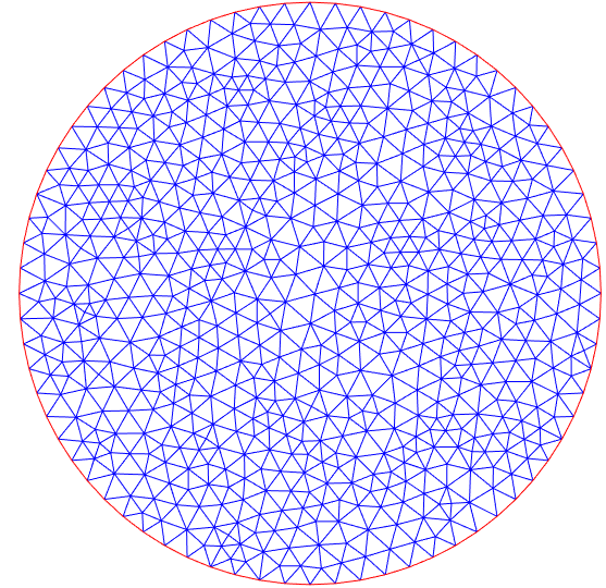
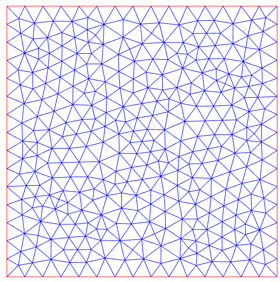
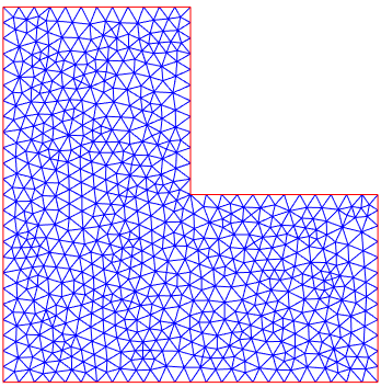
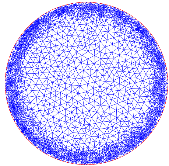
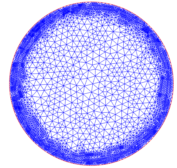
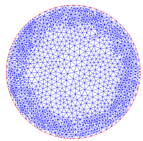
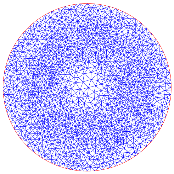
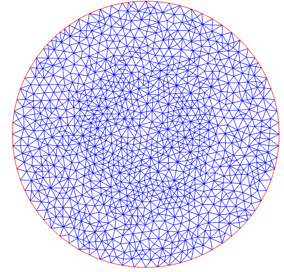
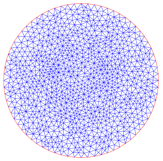
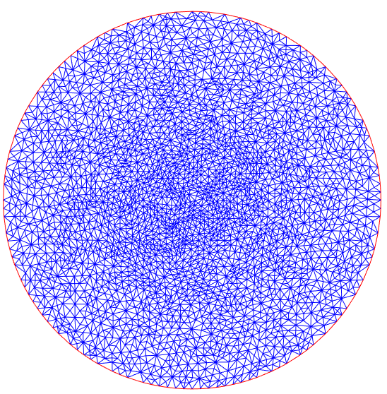
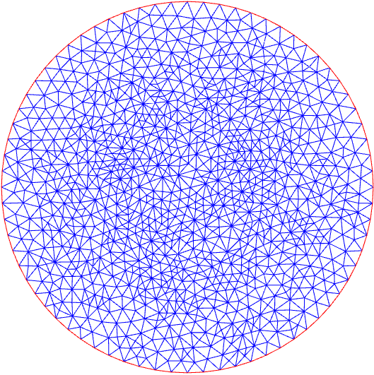
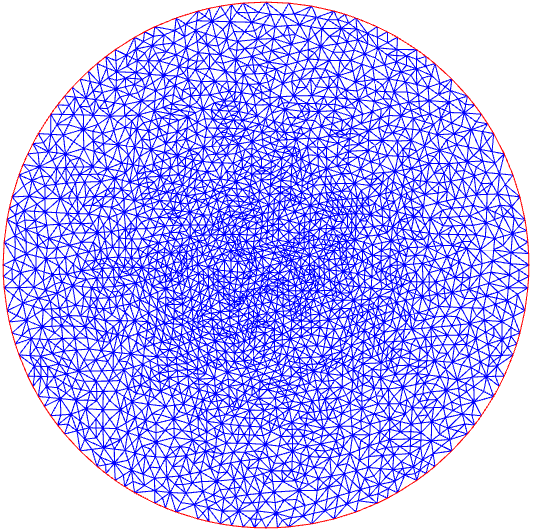
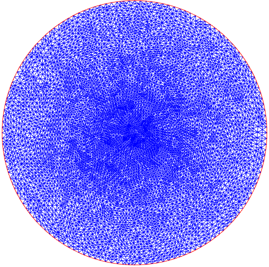
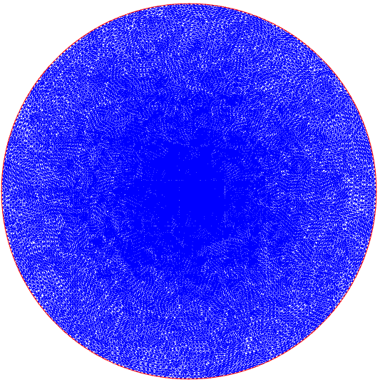
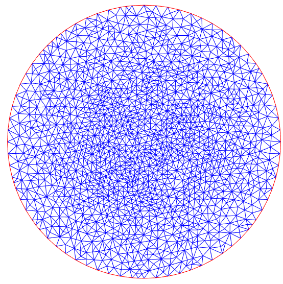
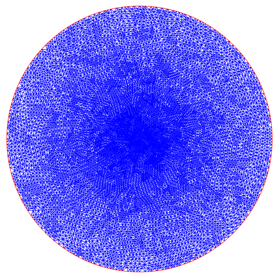
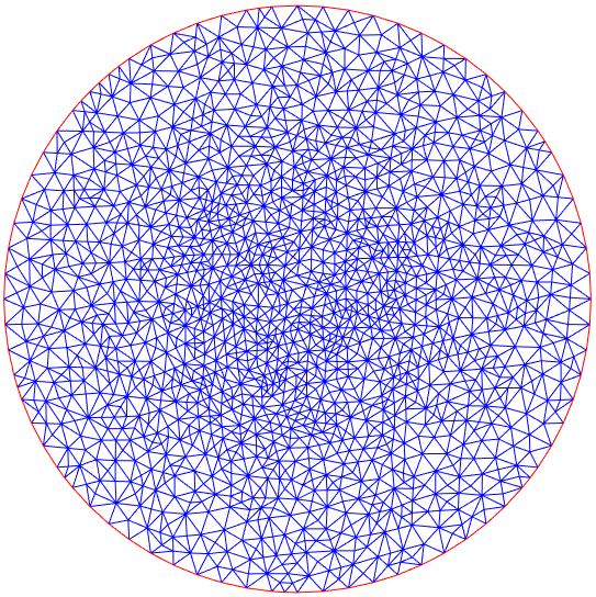
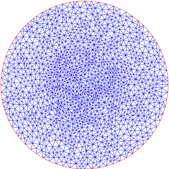
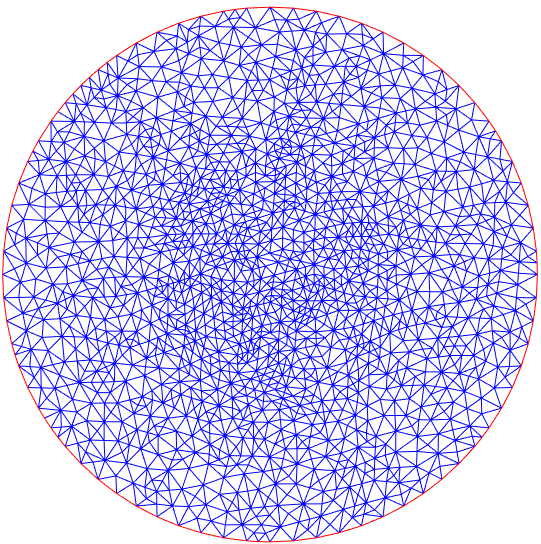
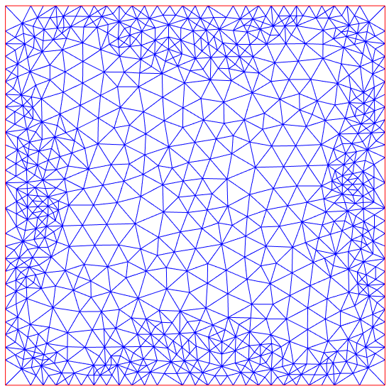
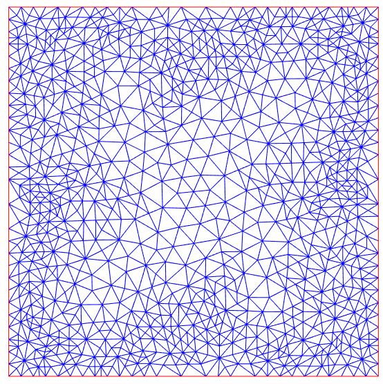
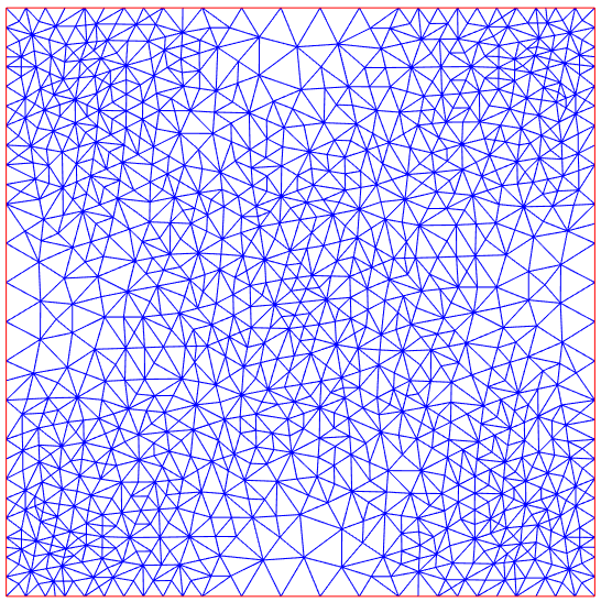
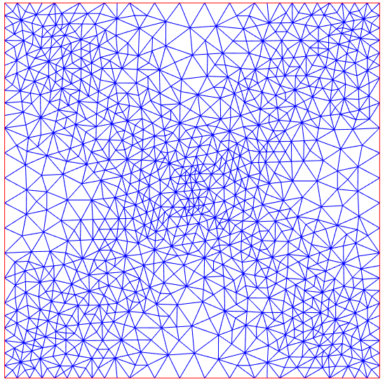
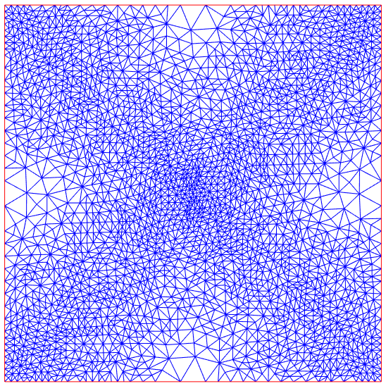
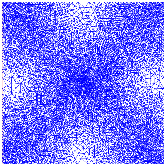
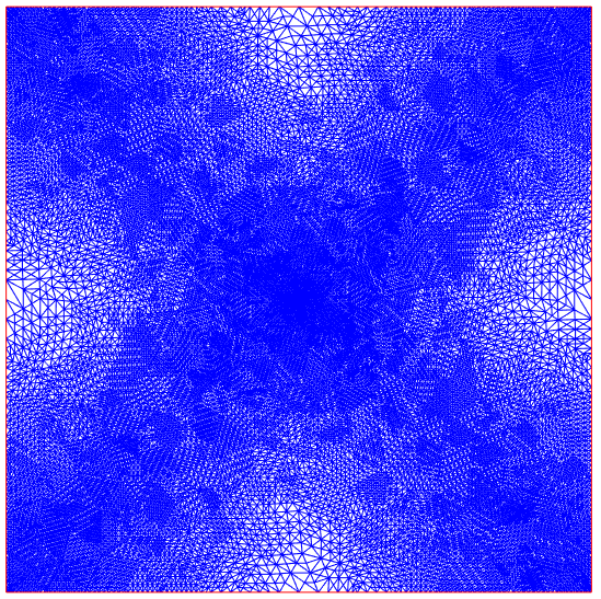
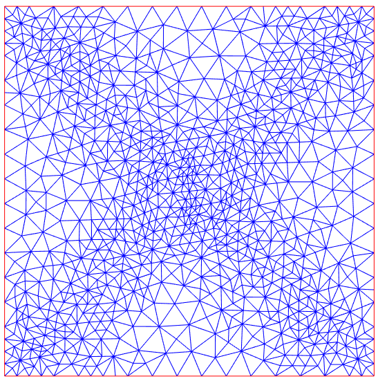
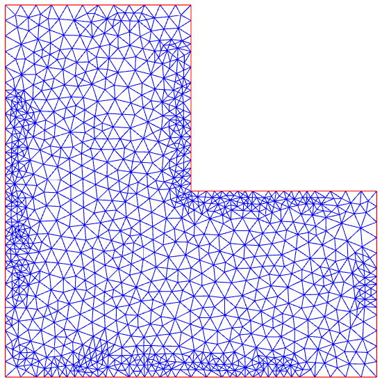
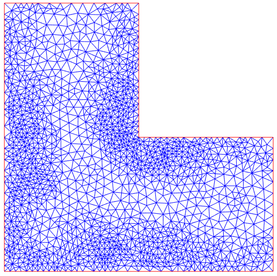
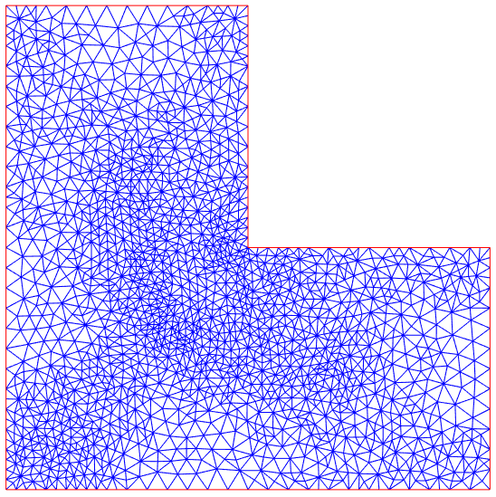
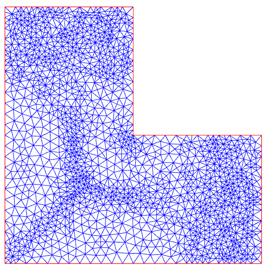
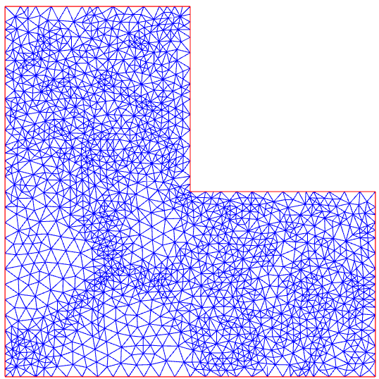
In all experiments, the module MARK of Algorithm 1 utilizing Dörfler’s strategy with $\theta=0.6$ yields a subset $\mathcal{M}_{k}$ such that $\eta_{k}(\mu_{k},u_{k},\mathcal{M}_{k})\geq 0.6\eta_{k}(\mu_{k},u_{k})$. Algorithm 1 proceeds until the relative error for two consecutive approximate eigenvalues is below a prescribed tolerance $\epsilon_{K}$, i.e., $|\mu_{k-1}-\mu_{k}|/\mu_{k-1}<\epsilon_{K}$. For large $p$, an upper bound $K$ is specified for the counter $k$ of adaptive refinement steps. In Algorithm 3, we set tolerance $\epsilon_{N}=10^{-5}$, and each component of $\bm{\xi}_{1}$ and $\bm{\nu}_{0}$ is an independent sample following the uniform distribution $U(0,0.5)$. Figure 1 displays three initial meshes used in Examples 5.1-5.3.

(a) $\mathcal{T}_{0}$ (682) in Example 5.1

(b) $\mathcal{T}_{0}$ (365) in Example 5.2

(c) $\mathcal{T}_{0}$ (741) in Example 5.3

Figure 1: Initial meshes ($k=0$) with the number of vertices in Examples 5.1-5.3.

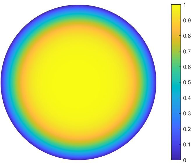
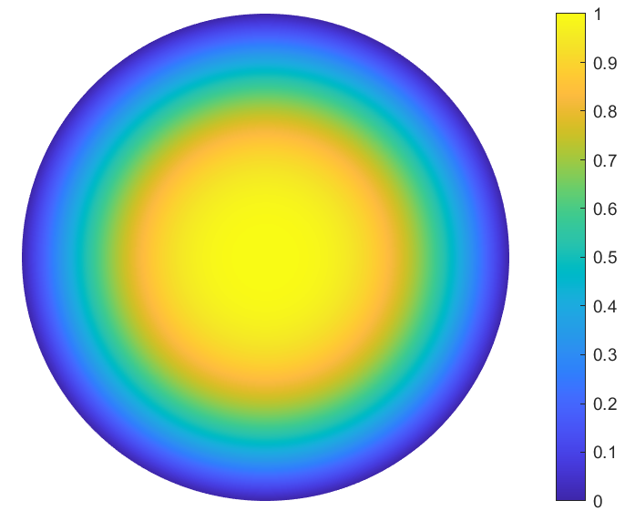
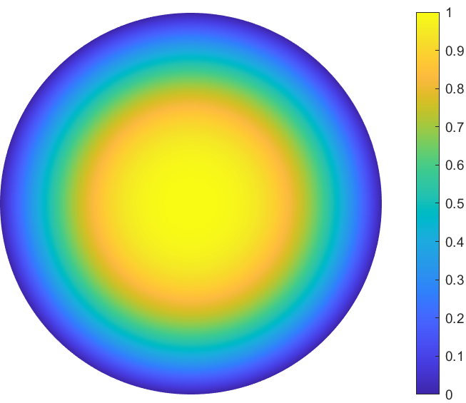
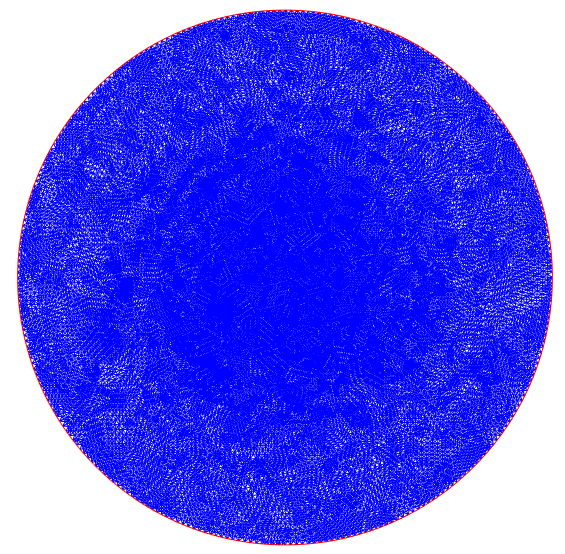
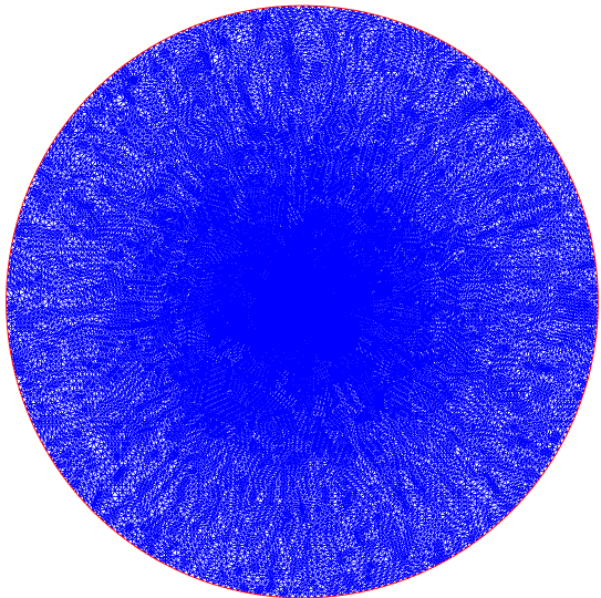
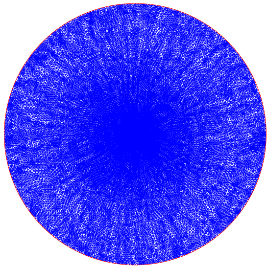
Example 5.1 (Unit Disk).

In the first example, the computational domain is a unit disk centered at the origin. Numerical experiments are implemented for 10 different values of

$$p\in\{1.1,1.2,1.5,2,2.5,3,4,10,20,30\}.$$

Tolerance $\epsilon_{K}$ in Algorithm 1 is set to be $5\times 10^{-4}$ for $p=1.1$ and $10^{-4}$ for the remaining cases, among which the adaptive algorithm terminates if the counter $k\geq K=9$ for $p=10,20,30$, while tolerance $\epsilon_{M}$ in Algorithm 2 is $10^{-5}$ for $p=1.5,2,2.5$ and $5\times 10^{-5}$ for the rest.

For each $p$, approximate values, over meshes generated by the adaptive strategy, of the 1st eigenvalue of (1.1) are provided in Table 1 ($p=1.1,1.2,1.5,2,2.5$) and Table 2 ($p=3,4,10,20,30$), where $k$ stands for the iteration number in Algorithm 1 while $\mu_{k}$ represents the approximate first eigenvalue over the $k$-th adaptive mesh. The results computed on a finest mesh by the uniform refinement strategy are listed in the last row as reference solutions. We observe that the sequence of computed eigenvalues $\{\mu_{k}\}_{k\geq 0}$ is decreasing and approaches the reference solution for each $p$ as the adaptive mesh refinement level $k$ increases. This numerical observation confirms the convergence of Algorithm 1 as proved in Theorem 4.3. One sees from Table 1 that the approximate eigenvalue $\mu_{8}=7.7111$ for $p=2.5$ is smaller than the reference solution produced by the uniform refinement, which implies more accuracy with fewer degrees of freedom of Algorithm 1. We observe similar behavior for $p=20,30$ in Table 2.

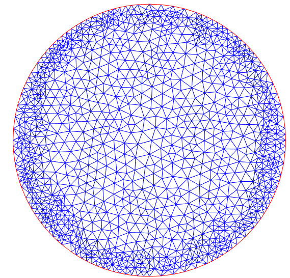
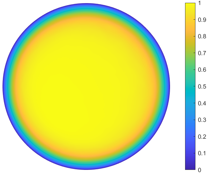
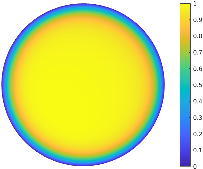
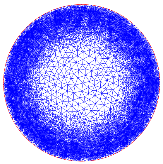
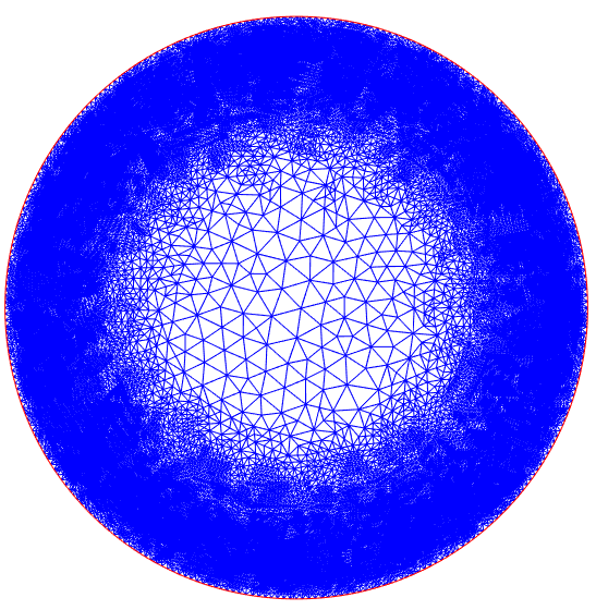
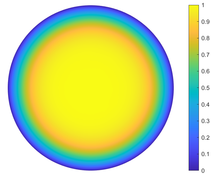
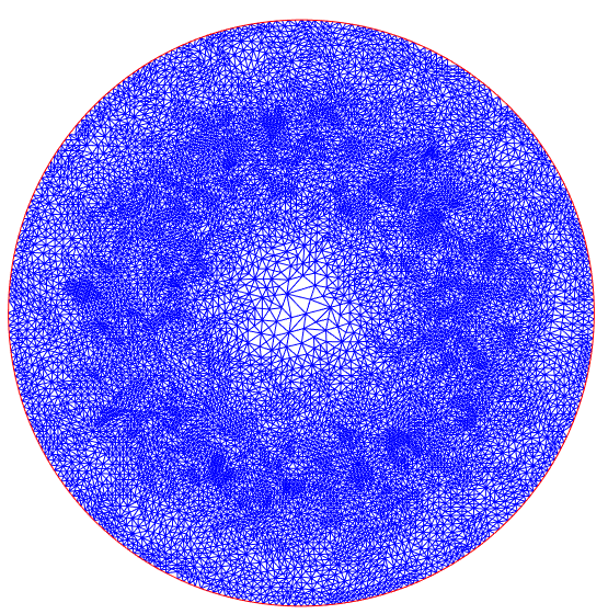
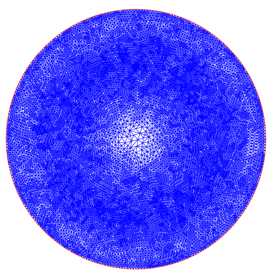
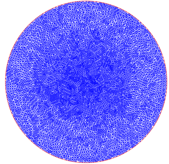
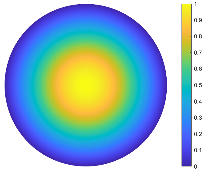
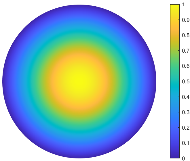
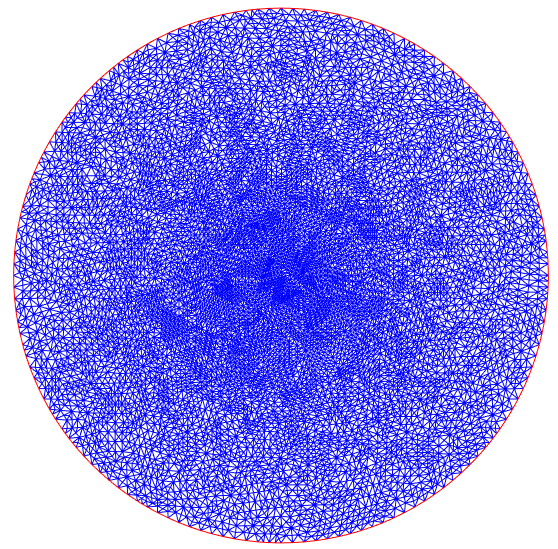
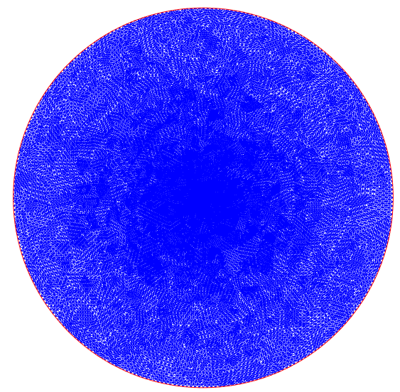
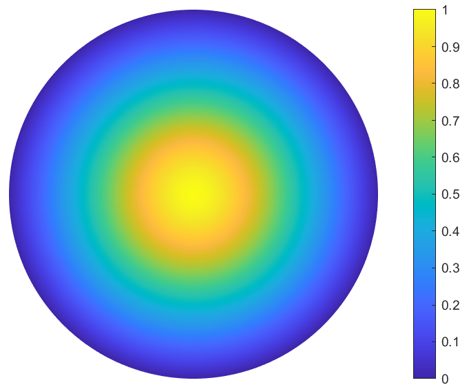
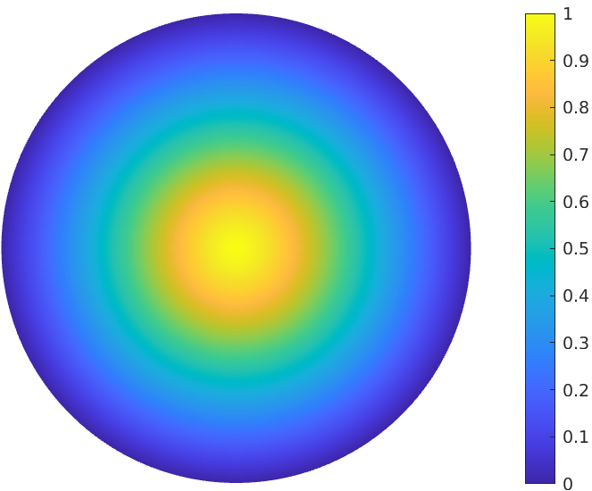
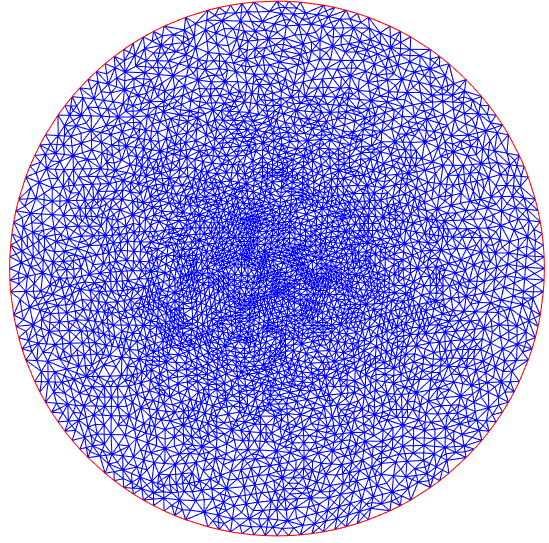
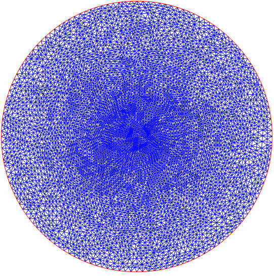
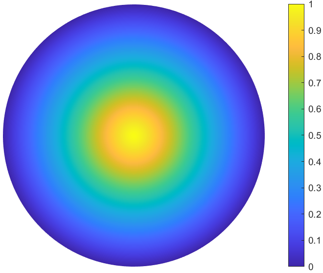
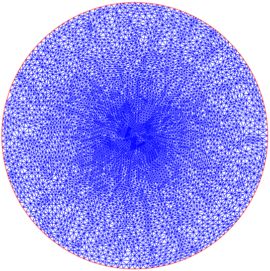
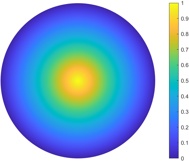
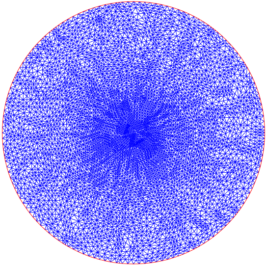
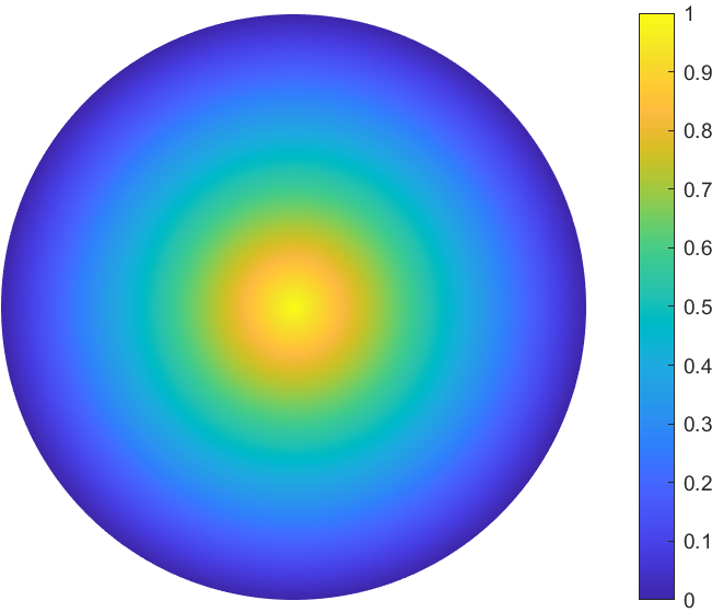
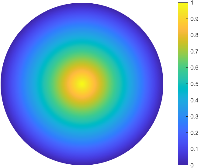
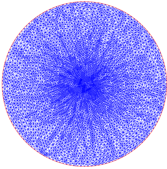
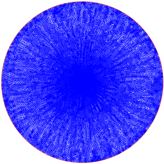
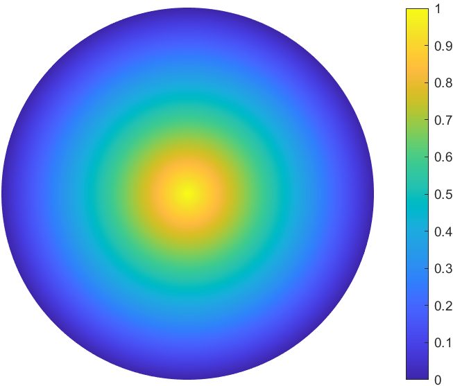
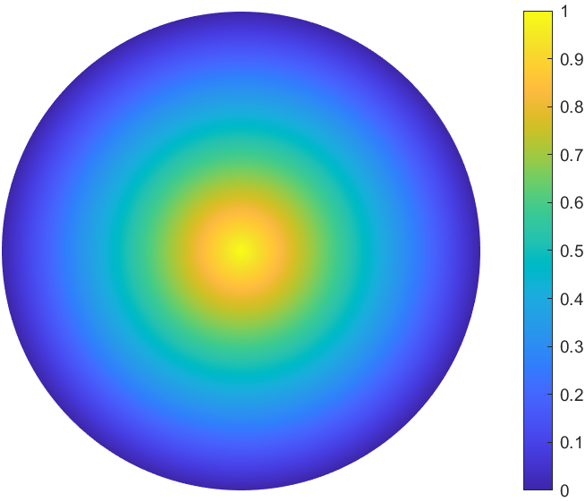
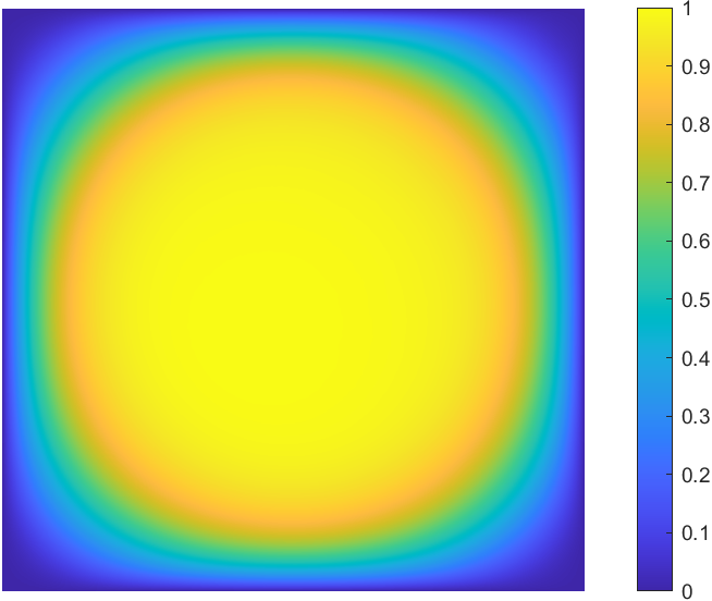
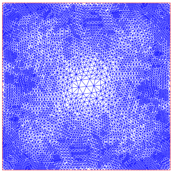
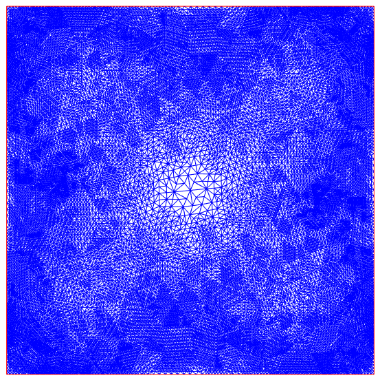
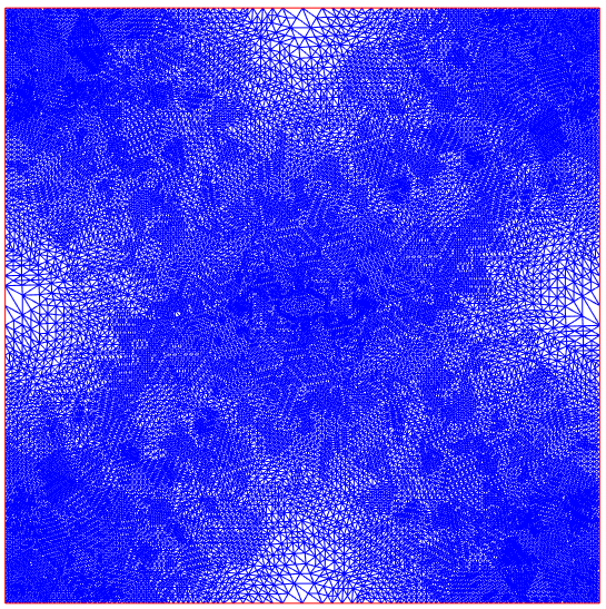
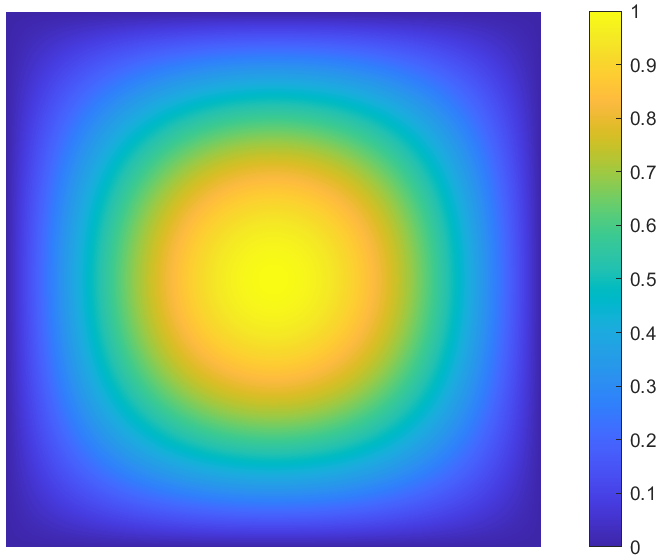
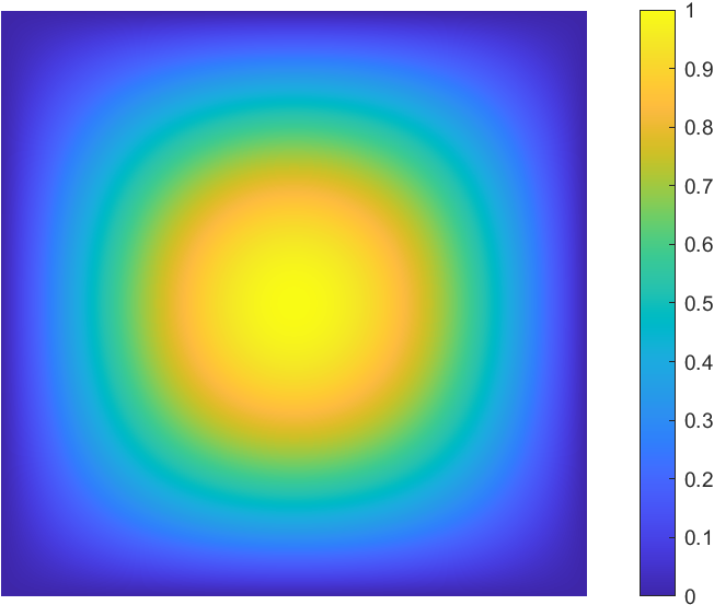
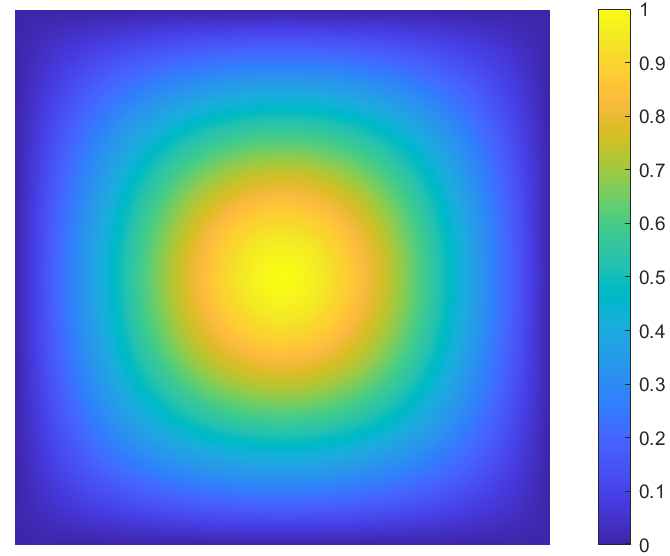
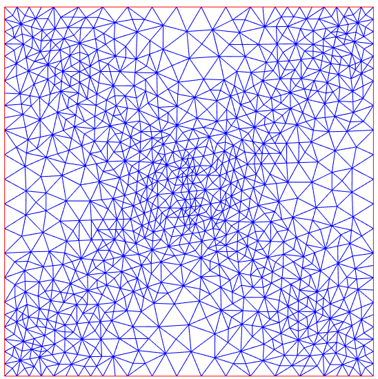
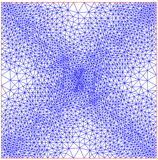
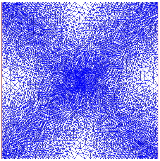
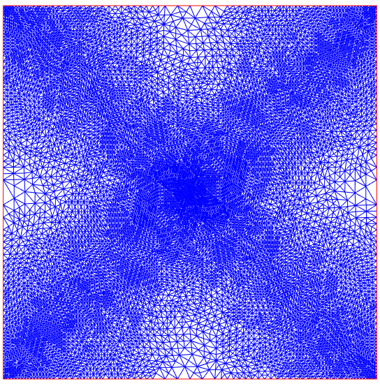
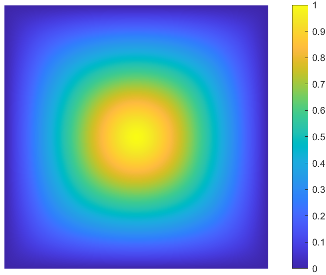
Figures 2-4 depict a selection of adaptive meshes generated by Algorithm 1 and computed first eigenfunctions over the finest adaptive meshes. For comparison, computed first eigenfunctions over uniformly refined meshes are displayed in the last column of Figures 2 and 4. We observe that local mesh refinements mainly occur in the region adjacent to the boundary for small $p$ and as $p$ becomes larger, more refinements are performed in the vicinity of the origin. Moreover, as can be seen from the penultimate column of Figure 2 (Figures 2(d)-2(s)), the last column of Figure 3 (Figures 3(e)-3(o)) and the penultimate column of Figure 4 (Figures 4(d)-4(n)), the asymptotic behaviour of adaptively computed first eigenfunctions confirms two assertions in [42] and [41] that the first $L^{\infty}(\Omega)$-normalized eigenfunction of (1.1) converges to 1, the characteristic function of the unit ball, as $p\rightarrow 1^{+}$ and to the distance function to the boundary, $1-\sqrt{x_{1}^{2}+x_{2}^{2}}$, as $p\rightarrow\infty$ respectively. This also explains the transition of additional mesh refinements from the boundary to the center.

Table 1: Quantitative result for $p\in\{1.1,1.2,1.5,2,2.5\}$ in Example 5.1: the number of adaptive loops, the number of vertices and the computed first eigenvalue.

$k$	$p=1.1$		$p=1.2$		$p=1.5$		$p=2$		$p=2.5$
	vertices	$\mu_{k}$	vertices	$\mu_{k}$	vertices	$\mu_{k}$	vertices	$\mu_{k}$	vertices	$\mu_{k}$
0	682	2.5773	682	2.9737	682	4.0294	682	5.8063	682	7.7529
1	909	2.5746	1044	2.9714	1225	4.0271	1196	5.8015	1154	7.7450
2	1305	2.5717	1693	2.9695	2268	4.0240	2091	5.7960	2002	7.7339
3	1965	2.5700	2909	2.9681	4064	4.0209	3721	5.7901	3480	7.7250
4	3136	2.5687	4965	2.9667	7278	4.0195	6532	5.7872	6157	7.7176
5	5088	2.5681	8806	2.9664	13150	4.0188	11639	5.7854	10838	7.7157
6			15564	2.9657	23147	4.0185	20538	5.7844	19258	7.7127
7			27492	2.9652			35714	5.7840	33969	7.7115
8			48994	2.9650					60310	7.7111
uniform	24505	2.5664	65130	2.9650	65130	4.0179	65130	5.7834	65130	7.7112

Table 2: Quantitative result for $p\in\{3,4,10,20,30\}$ Example 5.1: the number of adaptive loops, the number of vertices and the computed first eigenvalue.

$k$	$p=3$		$p=4$		$p=10$		$p=20$		$p=30$
	vertices	$\mu_{k}$	vertices	$\mu_{k}$	vertices	$\mu_{k}$	vertices	$\mu_{k}$	vertices	$\mu_{k}$
0	682	9.9049	682	14.8676	682	65.5544	682	270.4698	682	791.5021
1	1122	9.8894	1080	14.8207	1043	64.0777	1042	246.2074	1054	646.1338
2	1919	9.8724	1805	14.7780	1692	62.5367	1685	225.0614	1699	537.4712
3	3264	9.8542	3017	14.7333	2748	62.0430	2731	216.0264	2743	491.8927
4	5729	9.8418	5254	14.7100	4619	61.4137	4534	209.0268	4533	458.2254
5	10038	9.8382	9084	14.6939	7935	61.1213	7675	205.4670	7578	441.7788
6	17827	9.8357	16008	14.6939	13382	60.9851	12581	203.3949	12321	432.0333
7	31322	9.8355			22927	60.6762	21097	202.188	20458	427.0961
8					38617	60.8209	34565	201.4937	33063	424.5050
9					64689	60.7514	55859	201.4116	52812	422.9218
uniform	65130	9.8348	65130	14.6927	76492	60.6684	76492	201.6913	76492	423.1678

(a) $\mathcal{T}_{2}$ (1305)

(b) $\mathcal{T}_{4}$ (3136)

(c) $\mathcal{T}_{5}$ (5088)

(d) $u_{5}$

(e) uniform

(f) $\mathcal{T}_{2}$ (1693)

(g) $\mathcal{T}_{6}$ (15564)

(h) $\mathcal{T}_{8}$ (48994)

(i) $u_{8}$

(j) uniform

(k) $\mathcal{T}_{2}$ (2268)

(l) $\mathcal{T}_{5}$ (13150)

(m) $\mathcal{T}_{6}$ (23147)

(n) $u_{6}$

(o) uniform

(p) $\mathcal{T}_{1}$ (1196)

(q) $\mathcal{T}_{5}$ (11639)

(r) $\mathcal{T}_{7}$ (35714)

(s) $u_{7}$

(t) uniform

Figure 2: Adaptive mesh refinement level with the number of vertices over each mesh as well as final computed first eigenfunctions by adaptive and uniform refinements for $p=1.1,1.2,1.5,2$ in Example 5.1. $p=1.1$: 1st row, $p=1.2$: 2nd row, $p=1.5$: 3rd row and $p=2$: 4th row.

(a) $\mathcal{T}_{1}$ (1154)

(b) $\mathcal{T}_{3}$ (3480)

(c) $\mathcal{T}_{5}$ (10838)

(d) $\mathcal{T}_{7}$ (33969)

(e) $u_{8}$

(f) $\mathcal{T}_{1}$ (1122)

(g) $\mathcal{T}_{3}$ (3264)

(h) $\mathcal{T}_{5}$ (10038)

(i) $\mathcal{T}_{7}$ (31322)

(j) $u_{7}$

(k) $\mathcal{T}_{2}$ (1805)

(l) $\mathcal{T}_{4}$ (5254)

(m) $\mathcal{T}_{5}$ (9084)

(n) $\mathcal{T}_{6}$ (16008)

(o) $u_{6}$

Figure 3: Adaptive mesh refinement level with the number of vertices over each mesh as well as final computed first eigenfunctions by adaptive refinements for $p=2.5,3,4$ in Example 5.1. $p=2.5$: 1st row, $p=3$: 2nd row and $p=4$: 3rd row.

(a) $\mathcal{T}_{2}$ (1692)

(b) $\mathcal{T}_{5}$ (7935)

(c) $\mathcal{T}_{8}$ (38617)

(d) $u_{9}$

(e) uniform

(f) $\mathcal{T}_{2}$ (1685)

(g) $\mathcal{T}_{5}$ (7675)

(h) $\mathcal{T}_{8}$ (34565)

(i) $u_{9}$

(j) uniform

(k) $\mathcal{T}_{2}$ (1699)

(l) $\mathcal{T}_{5}$ (4533)

(m) $\mathcal{T}_{8}$ (33063)

(n) $u_{9}$

(o) uniform

Figure 4: Adaptive mesh refinement level with the number of vertices over each mesh as well as final computed first eigenfunctions by adaptive and uniform refinements for $p=10,20,30$ in Example 5.1. $p=10$: 1st row, $p=20$: 2nd row and $p=30$: 3rd row.

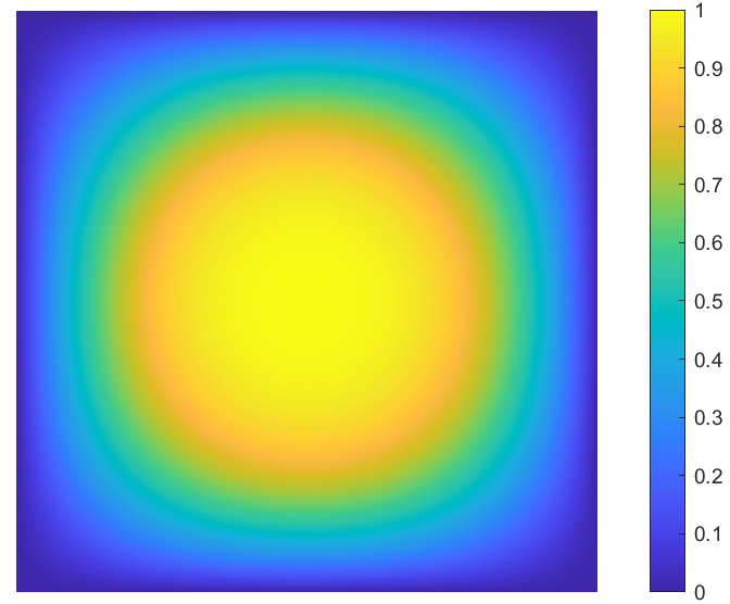
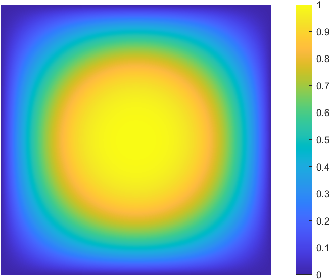
Example 5.2 (Unit Square).

We next consider the first eigenpair of (1.1) in a unit square $(0,1)^{2}$ with $p=1.2,1.5,2,2.5,3,4,10,20,30$. Tolerance $\epsilon_{K}$ in Algorithm 1 is chosen as $10^{-4}$ for all $p$ with maximum adaptive refinement number $K=11$ imposed for $p=10,20,30$ while $\epsilon_{M}=10^{-5}$ in Algorithm 2 except for $p=1.2$ and $p=4$, in both of which $\epsilon_{M}=5\times 10^{-5}$.

Table 3 and Table 4 contain all computed first eigenvalues over adaptively generated meshes and uniformly refined meshes. As in the previous example, the sequence of adaptive eigenvalues for each $p$ strictly decreases to the reference solution. Noting that the exact first eigenvalue of Laplacian ($p=2$) in the unit square is $2\pi^{2}=19.7392$, we see that our result $\mu_{9}=19.7410$ has an relative error less than $10^{-4}$.

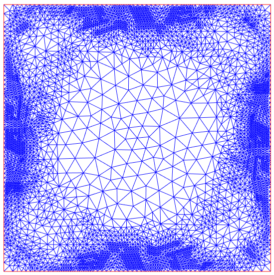
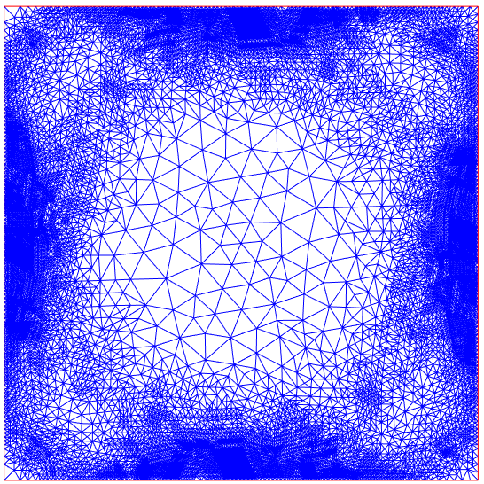
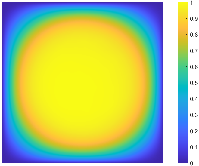
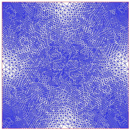
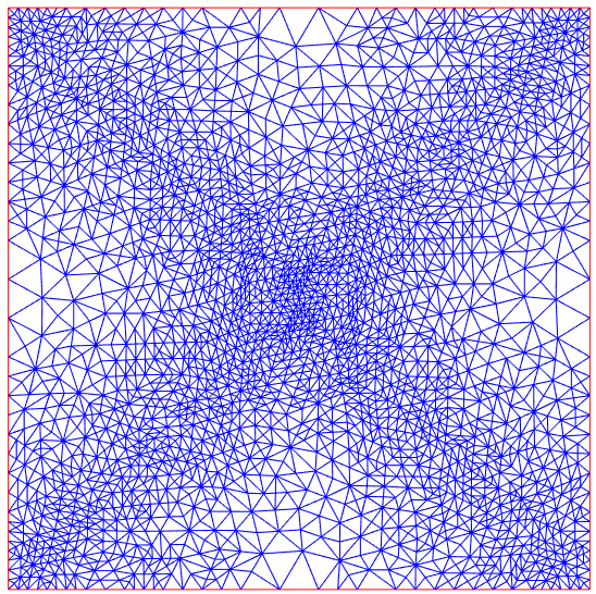
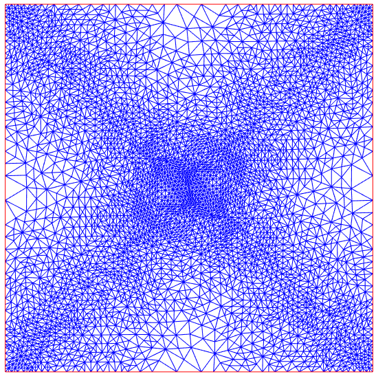
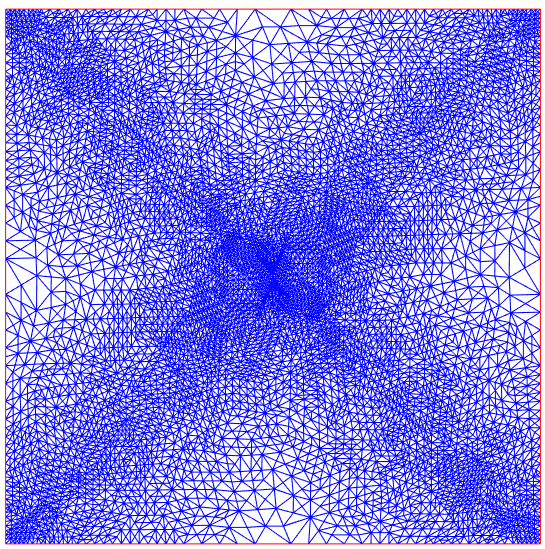
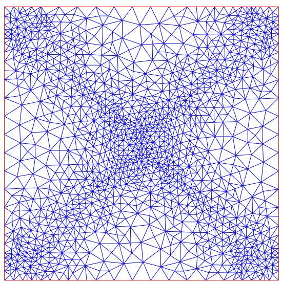
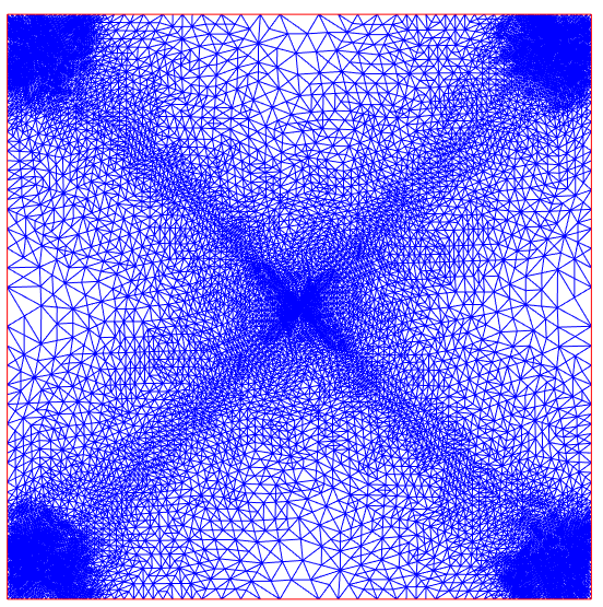
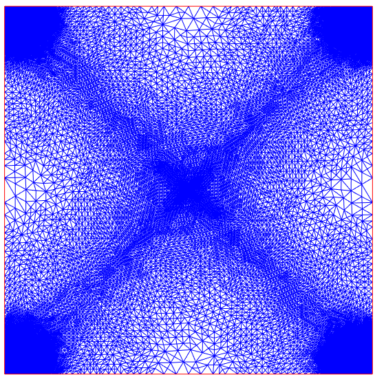
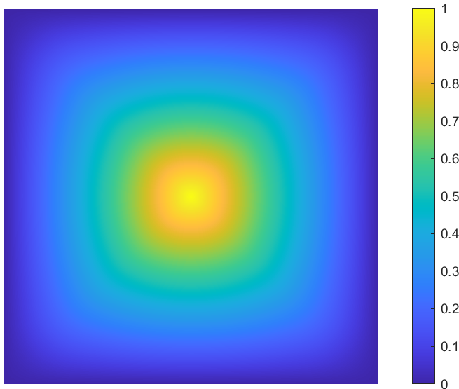
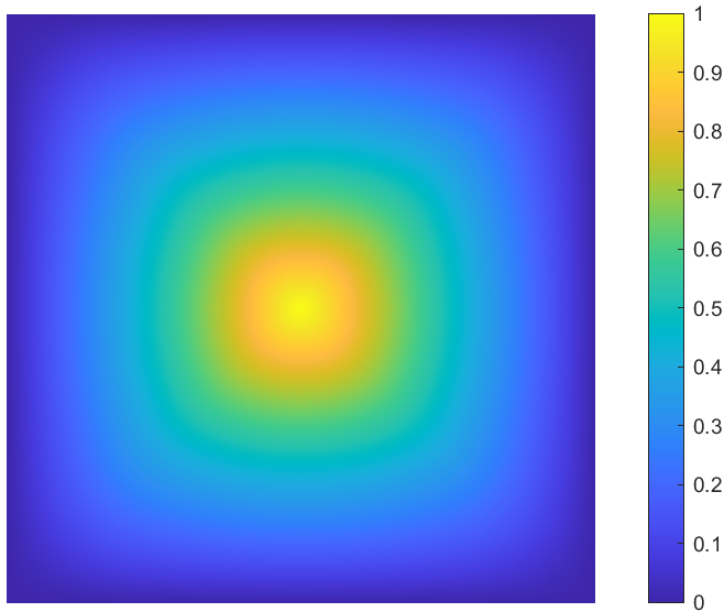
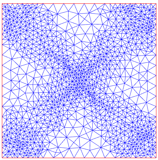
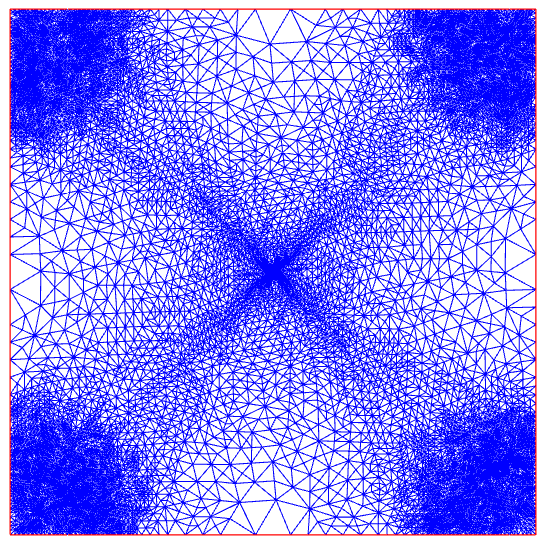
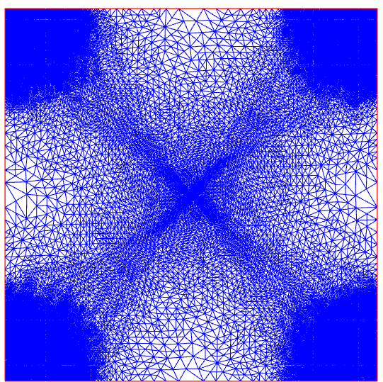
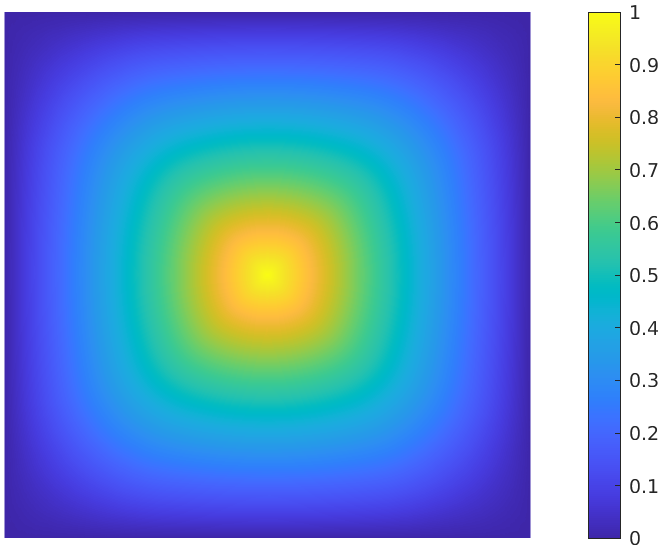
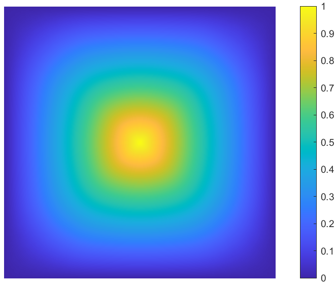
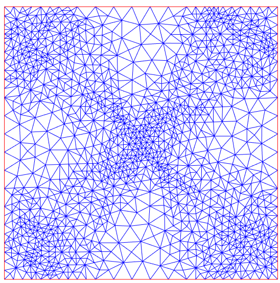
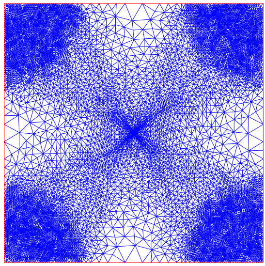
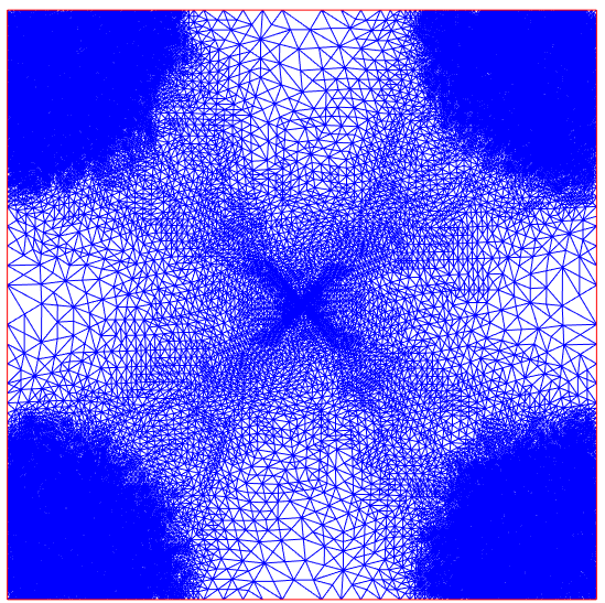
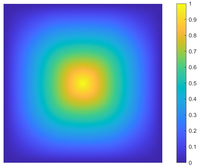
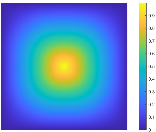
Sequences of adaptive meshes and computed first eigenfunctions over the finest adaptive meshes and uniformly refined meshes are displayed in Figures 5-7. The mesh is essentially refined near the boundary as before for small $p$ and then near two crossing diagonals for large $p$. As stated in [42], the first eigenvalue of $p$-Laplacian converges to the Cheeger constant of $\Omega$ as $p\rightarrow 1^{+}$ and the characteristic function of the Cheeger domain is the associated eigenfunction of $1$-Laplacian. In the current case that $\Omega=(0,1)^{2}$, the Cheeger domain is the unit square with each of its four corners rounded off by circular arcs of radius $1/(2+\sqrt{\pi})$ (after scaling) [42]. The computed first eigenfunction in Figure 5(d) is obviously an approximation of the characteristic function of the relevant Cheeger domain and more refinements naturally appear near the boundary (Figures 5(a)-5(c)) due to the large gradient of the analytic solution. On the other hand, further inspection of Figures 7(k)-7(m) for $p=30$ reveals that refinements are largely performed towards singularities in the vicinity of the center and around four corner points. The former observation indirectly confirms the assertion in a recent paper [15] that the $\infty$-ground state, as the limit of the first eigenfunction of $p$-Laplacian when $p\rightarrow\infty$, is $\infty$-harmonic in the viscosity sense and further continuously differentiable [52] in the unit square except on two diagonal segments lying in a symmetric neighbourhood around the center. As for the latter restriction of more refinements around four corner points, it is partially due to the boundary differentiability of a continuous $\infty$-harmonic function in [38] with $\partial\Omega$ and the boundary data being both continuously differentiable.

Table 3: Quantitative result for $p\in\{1.2,1.5,2,2.5,3\}$ in Example 5.2: the number of adaptive loops, the number of vertices and the computed first eigenvalue.

$k$	$p=1.2$		$p=1.5$		$p=2$		$p=2.5$		$p=3$
	vertices	$\mu_{k}$	vertices	$\mu_{k}$	vertices	$\mu_{k}$	vertices	$\mu_{k}$	vertices	$\mu_{k}$
0	365	6.2553	365	10.1425	365	19.8951	365	36.3173	365	63.6013
1	513	6.2349	595	10.1180	637	19.8497	610	36.2222	601	63.3666
2	841	6.2194	1049	10.1004	1083	19.8148	1071	36.1222	1048	63.1374
3	1290	6.2115	1799	10.0886	1885	19.7843	1861	36.0559	1799	62.9947
4	2237	6.2071	3226	10.0822	3257	19.7670	3224	36.0115	3142	62.9057
5	3543	6.2026	5681	10.0776	5640	19.7552	5702	35.9826	5477	62.8658
6	6213	6.2007	10013	10.0760	9908	19.7484	10107	35.9716	9526	62.7789
7	10424	6.1983	17476	10.0742	17197	19.7445	17543	35.9605	16513	62.7748
8	18114	6.1982	30561	10.0730	29834	19.7424	30645	35.9553
9			53957	10.0727	51244	19.7410	52987	35.9538
uniform	23972	6.1961	61431	10.0723	61431	19.7400	61431	35.9473	61431	62.7522

Table 4: Quantitative result for $p\in\{4,10,20,30\}$ in Example 5.2: the number of adaptive loops, the number of vertices and the computed first eigenvalue.

$k$	$p=4$		$p=10$		$p=20$		$p=30$
	vertices	$\mu_{k}$	vertices	$\mu_{k}$	vertices	$\mu_{k}$	vertices	$\mu_{k}$
0	365	180.4792	365	40150.9484	365	131552859.5567	365	316369444501.9748
1	591	179.2409	559	38480.8875	550	114754494.0675	573	247920190725.1581
2	998	178.2333	917	37311.8993	886	105284458.9813	904	214084636207.6707
3	1693	177.6302	1485	36821.6704	1407	101478437.2928	1458	200738781837.1732
4	2928	177.2105	2459	36423.1410	2283	98280542.2665	2317	189365323510.2901
5	5044	176.9028	4017	36218.4984	3592	96469391.6877	3720	181254359971.9188
6	8673	176.8865	6366	36080.0603	5647	95344022.9545	5863	177296955151.1784
7			9896	36006.8163	8944	94532337.2298	9301	174106568619.4988
8			14942	35959.9800	13968	93821101.8889	14736	171834680280.8138
9			22442	35923.8812	21966	93383333.7755	23223	170184024746.6412
10			34016	35913.7856	34745	93034451.0330	36868	168828158945.8095
11			52132	35885.7953	54919	92733351.0224	58498	167506820586.1468
uniform	61431	176.7496	69177	35858.9478	69177	92553599.6382	69177	167212825530.8619

(a) $\mathcal{T}_{2}$ (841)

(b) $\mathcal{T}_{6}$ (6213)

(c) $\mathcal{T}_{8}$ (18114)

(d) $u_{8}$

(e) uniform

(f) $\mathcal{T}_{2}$ (1049)

(g) $\mathcal{T}_{6}$ (10013)

(h) $\mathcal{T}_{8}$ (30561)

(i) $u_{9}$

(j) uniform

(k) $\mathcal{T}_{2}$ (1083)

(l) $\mathcal{T}_{6}$ (9908)

(m) $\mathcal{T}_{8}$ (29834)

(n) $u_{9}$

(o) uniform

Figure 5: Adaptive mesh refinement level with the number of vertices over each mesh as well as final computed first eigenfunctions by adaptive and uniform refinements for $p=1.2,1.5,2$ in Example 5.2. $p=1.2$: 1st row, $p=1.5$: 2nd row, $p=2$: 3rd row.

(a) $\mathcal{T}_{2}$ (1071)

(b) $\mathcal{T}_{4}$ (3224)

(c) $\mathcal{T}_{6}$ (10107)

(d) $\mathcal{T}_{8}$ (30645)

(e) $u_{9}$

(f) $\mathcal{T}_{2}$ (1048)

(g) $\mathcal{T}_{4}$ (3142)

(h) $\mathcal{T}_{6}$ (9526)

(i) $\mathcal{T}_{7}$ (16513)

(j) $u_{7}$

(k) $\mathcal{T}_{2}$ (998)

(l) $\mathcal{T}_{4}$ (2928)

(m) $\mathcal{T}_{5}$ (5044)

(n) $\mathcal{T}_{6}$ (8673)

(o) $u_{6}$

Figure 6: Adaptive mesh refinement level with the number of vertices over each mesh as well as final computed first eigenfunctions by adaptive refinements for $p=2.5,3,4$ in Example 5.2. $p=2.5$: 1st row, $p=3$: 2nd row, $p=4$: 3rd row.

(a) $\mathcal{T}_{3}$ (1485)

(b) $\mathcal{T}_{8}$ (14942)

(c) $\mathcal{T}_{11}$ (52132)

(d) $u_{11}$

(e) uniform

(f) $\mathcal{T}_{3}$ (1407)

(g) $\mathcal{T}_{8}$ (13968)

(h) $\mathcal{T}_{11}$ (54919)

(i) $u_{11}$

(j) uniform

(k) $\mathcal{T}_{3}$ (1458)

(l) $\mathcal{T}_{8}$ (14736)

(m) $\mathcal{T}_{11}$ (58498)

(n) $u_{11}$

(o) uniform

Figure 7: Adaptive mesh refinement level with the number of vertices over each mesh as well as final computed first eigenfunctions by adaptive and uniform refinements for $p=10,20,30$ in Example 5.2. $p=10$: 1st row, $p=20$: 2nd row, $p=30$: 3rd row.

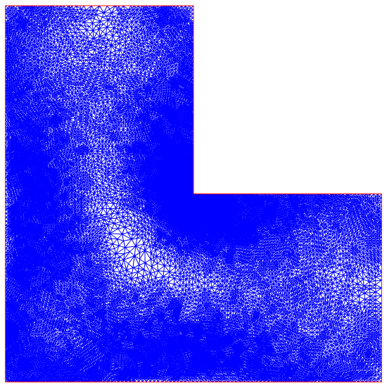
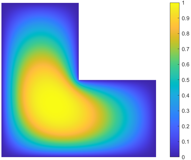
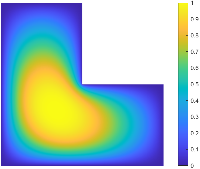
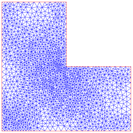
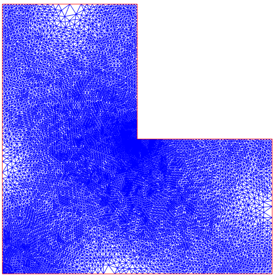
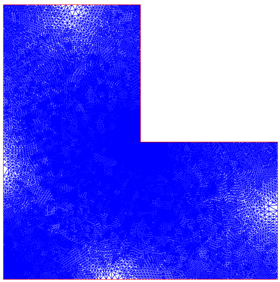
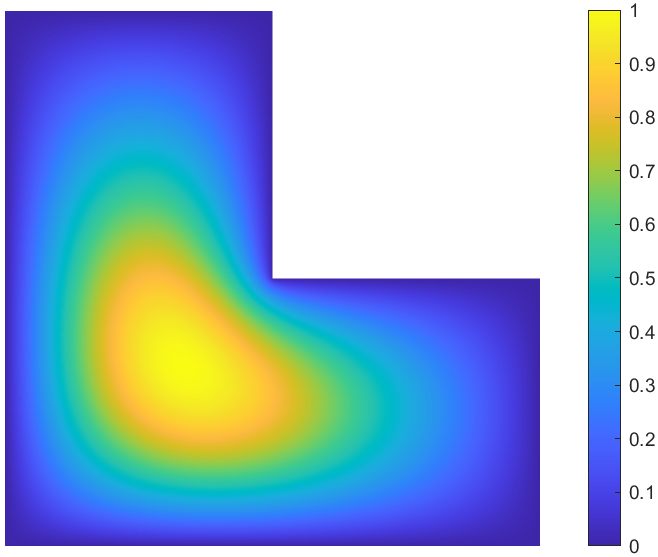
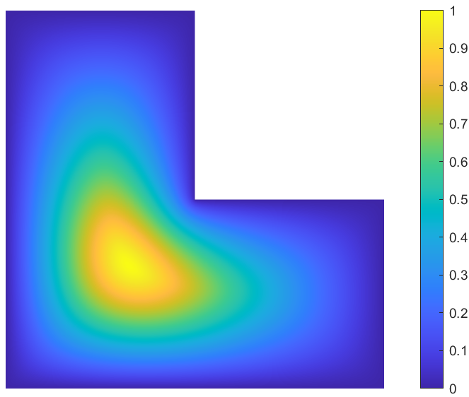
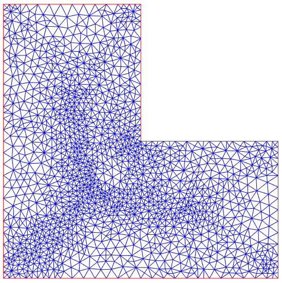
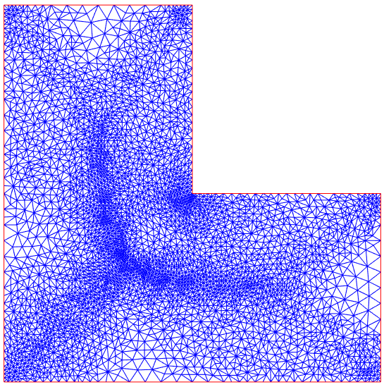
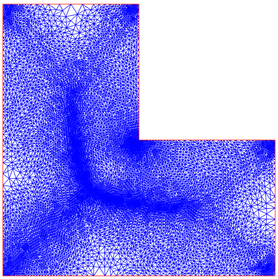
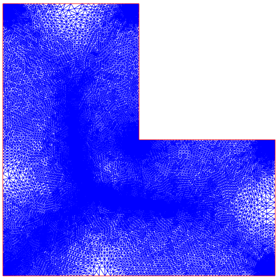
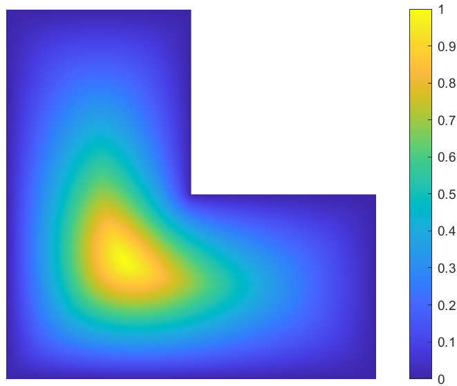
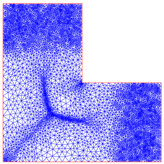
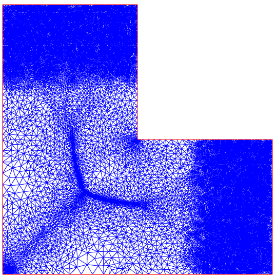
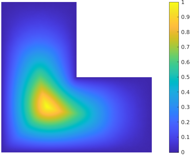
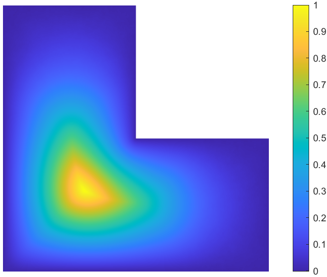
Example 5.3 (L-shaped domain).

The third example is posed in an L-shaped domain $(0,2)^{2}\setminus[1,2)^{2}$ with the same values of $p$ as in Example 5.1. Tolerances $\epsilon_{K}$ and $\epsilon_{M}$ are given by $10^{-4}$ and $10^{-5}$ for $p\in\{1.5,2,2.5,3\}$ and $5\times 10^{-4}$ and $5\times 10^{-5}$ for $p\in\{1.1,1.2,4,10,20,30\}$ respectively. A maximum iteration number $K=8$ is specified for $p=1.1,10,20,30$.

The convergence history of Algorithm 1 is presented in Tables 5 and 6, which show similar convergence behaviour of computed first eigenvalues for each $p$. Compared with the reference solution over the mesh by uniform refinements, fewer degrees of freedom by Algorithm 1 is required for more accuracy when $p$ is small. In particular, we observe from Table 6 with $p=4$ that the computed eigenvalues $\mu_{8}=54.6447$ and $\mu_{9}=54.6389$ by Algorithm 1, albeit with only $41\%$ and $67\%$ of degrees of freedom respectively, are both smaller than the reference solution by uniform refinements.

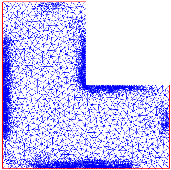
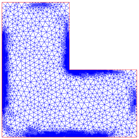
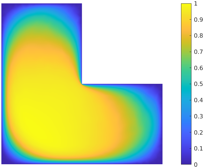
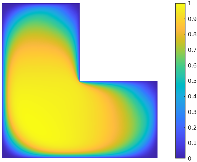
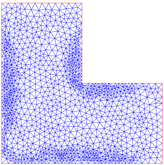
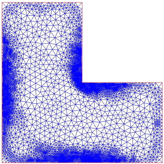
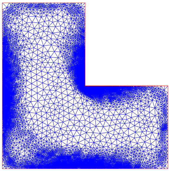
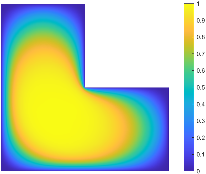
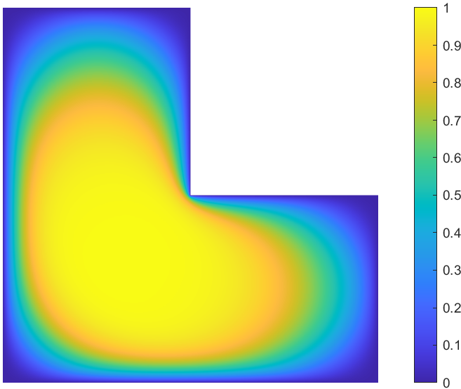
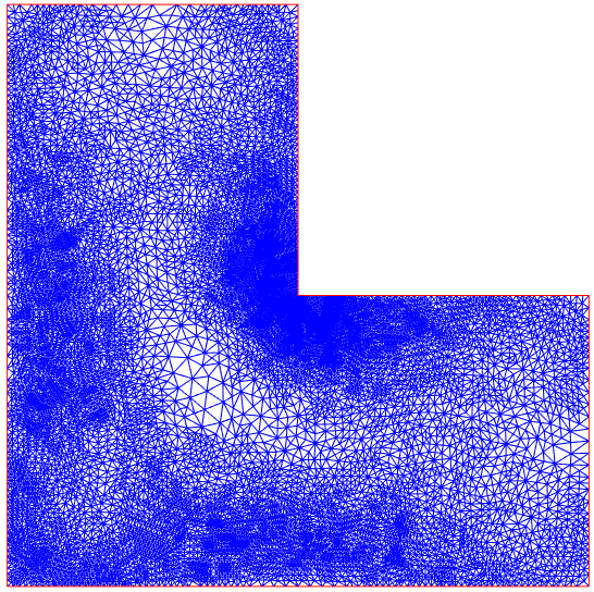
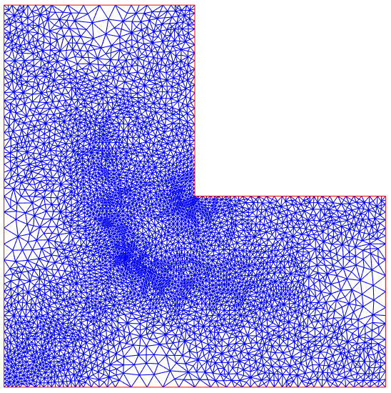
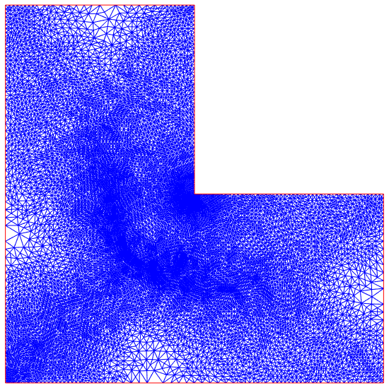
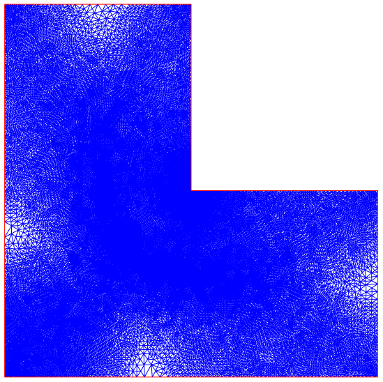
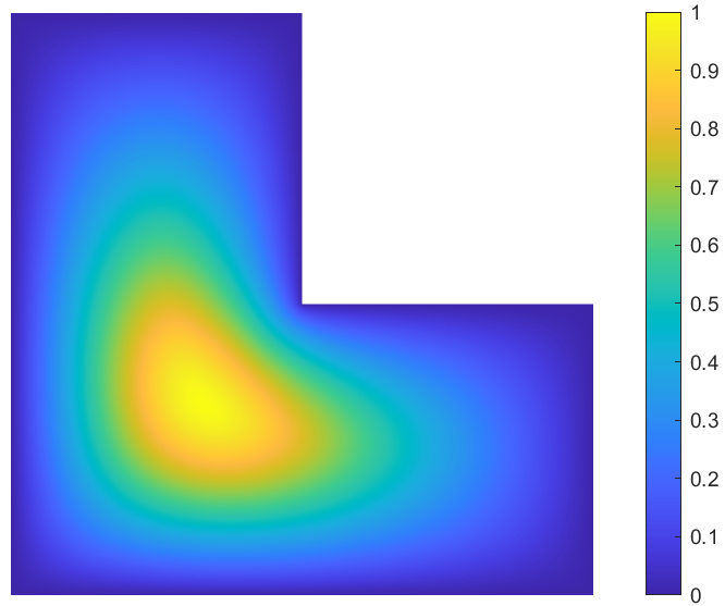
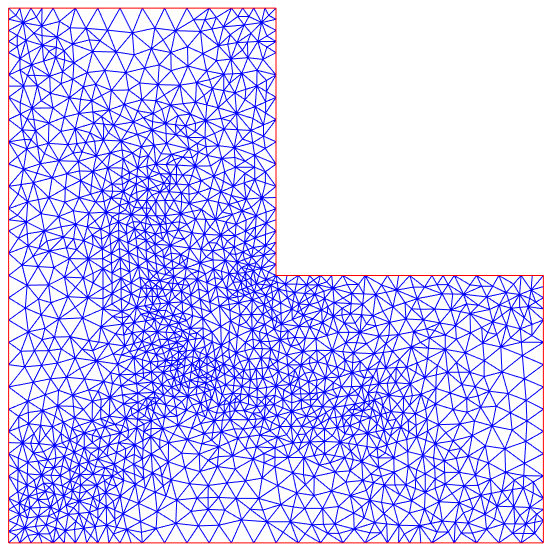
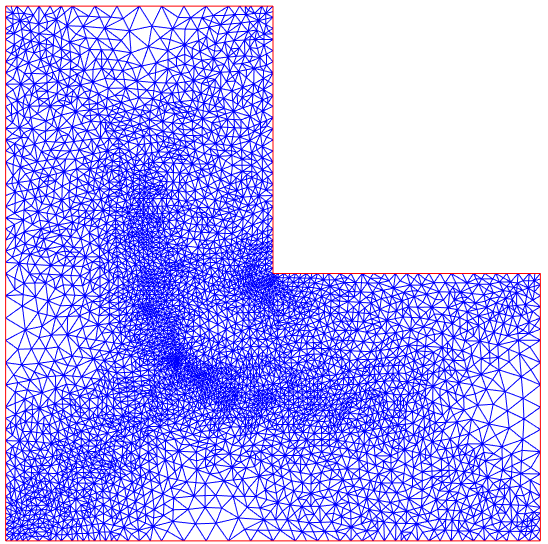
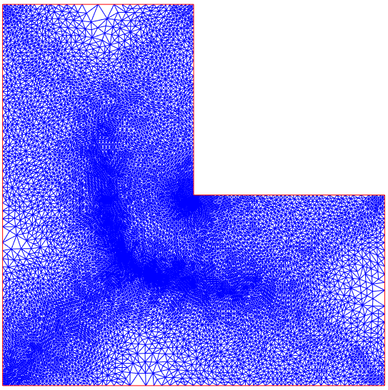
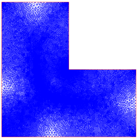
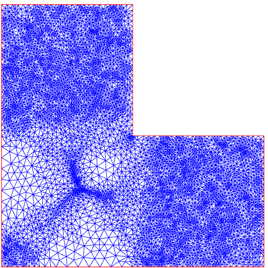
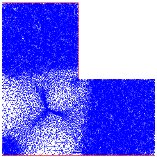
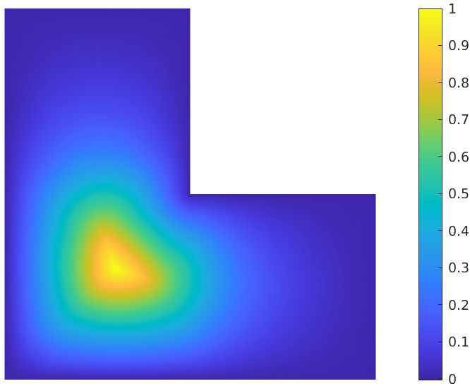
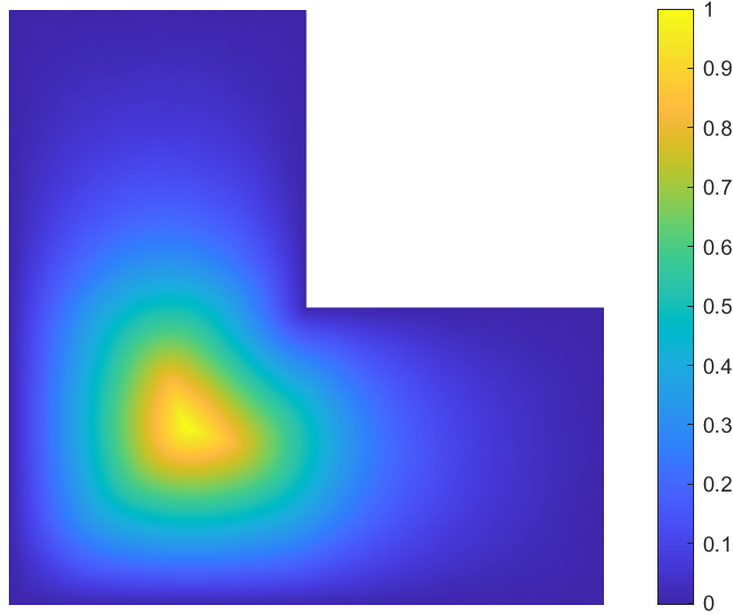
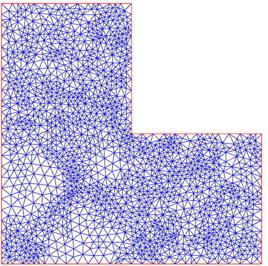
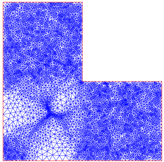
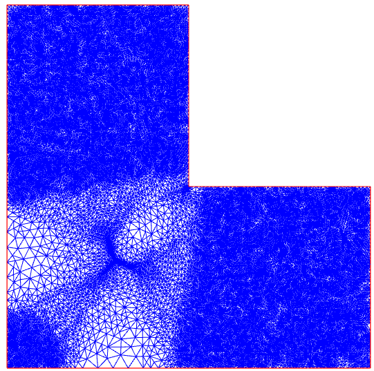
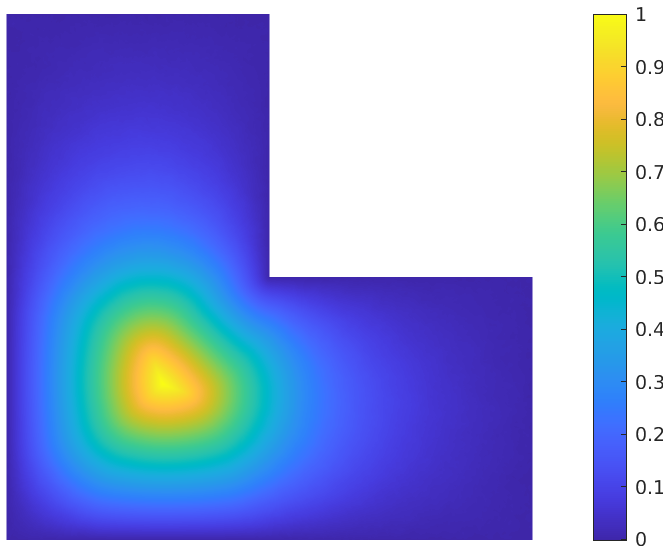
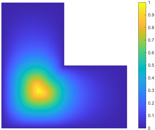
Figures 8-10 show that the marked regions from Algorithm 1 transfer from the region adjacent to the boundary to the vicinity of the origin as $p$ increases, and meanwhile the corner singularities are clearly detected for each $p$. From the penultimate column of Figure 8 (Figures 8(d)-8(s)), we may deduce as in Example 5.2 that the computed first eigenfunctions are approximations of the characteristic function associated with some Cheeger domain [42] as the first eigenfunction of 1-Laplacian in $\Omega$. What is intriguing in Figure 10 is that meshes are largely refined in the second quadrant and the fourth quadrant for large $p$, where the computed eigenfunctions are zero. To the best of our knowledge, no reasonable explanation of this observation is available in the PDE theory. This might provide a clue about the regularity of the $\infty$-eigenvalue problem in a non-convex domain.

Table 5: Quantitative result for $p\in\{1.1,1.2,1.5,2,2.5\}$ in Example 5.3: the number of adaptive loops, the number of vertices and the computed first eigenvalue.

$k$	$p=1.1$		$p=1.2$		$p=1.5$		$p=2$		$p=2.5$
	vertices	$\mu_{k}$	vertices	$\mu_{k}$	vertices	$\mu_{k}$	vertices	$\mu_{k}$	vertices	$\mu_{k}$
0	741	3.2931	741	3.9109	741	5.7422	741	9.7511	741	15.6655
1	923	3.2705	982	3.8894	1143	5.7170	1188	9.7100	1169	15.5842
2	1208	3.2594	1358	3.8797	1855	5.7053	1990	9.6861	1917	15.5368
3	1540	3.2542	1919	3.8730	3078	5.6969	3385	9.6684	3213	15.5009
4	2151	3.2502	2934	3.8698	5168	5.6922	5748	9.6575	5514	15.4794
5	2950	3.2492	4501	3.8656	8608	5.6887	9842	9.6506	9361	15.4665
6	4370	3.2463	7254	3.8641	14510	5.6860	16767	9.6465	16093	15.4565
7	6391	3.2439	11430	3.8621	23999	5.6849	28561	9.6439	27669	15.4512
8	10006	3.2432	18888	3.8614	40570	5.6838	48554	9.6422	47246	15.4479
9					68486	5.6836	82874	9.6413	81070	15.4464
10							140675	9.6407
uniform	20390	3.2402	23347	3.8617	81528	5.6840	209247	9.6410	92622	15.4480

Table 6: Quantitative result for $p\in\{3,4,10,20,30\}$ in Example 5.3: the number of adaptive loops, the number of vertices and the computed first eigenvalue.

$k$	$p=3$		$p=4$		$p=10$		$p=20$		$p=30$
	vertices	$\mu_{k}$	vertices	$\mu_{k}$	vertices	$\mu_{k}$	vertices	$\mu_{k}$	vertices	$\mu_{k}$
0	741	24.4193	741	56.1209	741	4317.3478	741	2708987.0461	741	1303851067.7577
1	1147	24.2634	1120	55.5759	1162	4131.3028	1199	2512492.6457	1236	1120643502.0261
2	1865	24.1657	1792	55.2164	1819	4017.6591	1915	2218019.0149	2022	905737323.1926
3	3096	24.0980	2935	54.9928	2898	3946.9782	3062	2134283.6656	3294	865477916.6093
4	5217	24.0562	4903	54.8456	4593	3910.2560	4895	2060551.9890	5252	787815753.7906
5	8811	24.0302	8198	54.7636	7309	3886.0046	7772	2029084.8475	8468	766028318.9108
6	15080	24.0104	13787	54.7045	11685	3864.2231	12427	1989540.7277	13570	737686838.7466
7	25795	23.9998	23016	54.6751	18698	3849.7642	19789	1969350.1740	21568	727425378.3108
8	44192	23.9954	38027	54.6447	29957	3837.6159	31633	1951449.9252	34516	713175988.2458
9	76011	23.9910	61810	54.6389
10	129671	23.9884
11	221634	23.9872
uniform	256870	23.9903	92622	54.6546	44439	3813.4477	44439	1924156.5406	44439	703152959.0755

(a) $\mathcal{T}_{2}$ (1208)

(b) $\mathcal{T}_{6}$ (4370)

(c) $\mathcal{T}_{8}$ (10006)

(d) $u_{8}$

(e) uniform

(f) $\mathcal{T}_{2}$ (1358)

(g) $\mathcal{T}_{6}$ (7254)

(h) $\mathcal{T}_{8}$ (18888)

(i) $u_{8}$

(j) uniform

(k) $\mathcal{T}_{2}$ (1855)

(l) $\mathcal{T}_{6}$ (14510)

(m) $\mathcal{T}_{8}$ (40570)

(n) $u_{9}$

(o) uniform

(p) $\mathcal{T}_{2}$ (1990)

(q) $\mathcal{T}_{6}$ (16767)

(r) $\mathcal{T}_{8}$ (48554)

(s) $u_{10}$

(t) uniform

Figure 8: Adaptive mesh refinement level with the number of vertices over each mesh as well as final computed first eigenfunctions by adaptive and uniform refinements for $p=1.1,1.2,1.5,2$ in Example 5.3. $p=1.1$: 1st row, $p=1.2$: 2nd row, $p=1.5$: 3rd row and $p=2$: 4th row.

(a) $\mathcal{T}_{2}$ (1917)

(b) $\mathcal{T}_{4}$ (5514)

(c) $\mathcal{T}_{6}$ (16093)

(d) $\mathcal{T}_{8}$ (47246)

(e) $u_{9}$

(f) $\mathcal{T}_{2}$ (1865)

(g) $\mathcal{T}_{4}$ (5217)

(h) $\mathcal{T}_{6}$ (15080)

(i) $\mathcal{T}_{8}$ (44192)

(j) $u_{11}$

(k) $\mathcal{T}_{2}$ (1792)

(l) $\mathcal{T}_{4}$ (4903)

(m) $\mathcal{T}_{6}$ (13787)

(n) $\mathcal{T}_{8}$ (38027)

(o) $u_{9}$

Figure 9: Adaptive mesh refinement level with the number of vertices over each mesh as well as final computed first eigenfunctions by adaptive refinements for $p=2.5,3,4$ in Example 5.2. $p=2.5$: 1st row, $p=3$: 2nd row, $p=4$: 3rd row.

(a) $\mathcal{T}_{2}$ (1819)

(b) $\mathcal{T}_{5}$ (7309)

(c) $\mathcal{T}_{8}$ (29957)

(d) $u_{8}$

(e) uniform

(f) $\mathcal{T}_{2}$ (1915)

(g) $\mathcal{T}_{5}$ (7772)

(h) $\mathcal{T}_{8}$ (31633)

(i) $u_{8}$

(j) uniform

(k) $\mathcal{T}_{2}$ (2022)

(l) $\mathcal{T}_{5}$ (8468)

(m) $\mathcal{T}_{8}$ (34516)

(n) $u_{8}$

(o) uniform

Figure 10: Adaptive mesh refinement level with the number of vertices over each mesh as well as final computed first eigenfunctions by adaptive and uniform refinements for $p=10,20,30$ in Example 5.3. $p=10$: 1st row, $p=20$: 2nd row, $p=30$: 3rd row.

6 Conclusions

An adaptive finite element method has been designed to approximate the first eigenvalue of the $p$-Laplacian operator. We have proved that the sequence of discrete eigenvalues and discrete eigenfunctions converges to the exact one and the related eigenset respectively with the help of minimization techniques in derivation of existence result for nonlinear elliptic equations. In the process, a residual-type error estimator is available and serves in the module ESTIMATE of the adaptive algorithm. The asymptotic behavior of computed 1st eigenfunctions shows that our adaptive algorithm can capture the singularities as described in the PDE theory. Since the conforming finite element method only provides an upper bound for the first eigenvalue, one natural question is how to yield a lower bound. One possible choice is the nonconforming finite element method, which works for $2$-Laplacian [5, 20, 40, 49, 50, 58]. In view of this, our future research topic is the study of an adaptive nonconforming method for the first eigenpair of $p$-Laplacian.

Funding

The research of Guanglian Li was partially supported by Hong Kong RGC through General Research Fund (project number: 17317122) and Early Career Scheme (project number: 27301921). The research of Yifeng Xu was partially supported by the National Natural Science Foundation of China (Projects 12250013, 12261160361 and 12271367), the Science and Technology Commission of Shanghai Municipality (Projects 20JC1413800 and 22ZR1445400) and a General Research Fund (KF202318) from Shanghai Normal University. The work of Shengfeng Zhu was partially supported by the National Key Basic Research Program under grant 2022YFA1004402 and the Science and Technology Commission of Shanghai Municipality (Projects 22ZR1421900 and 22DZ2229014).

References

- [1] R. Adams and J. Fournier, Sobolev Spaces, 2nd ed., Elsevier Science/Academic Press, Amsterdam, 2003.
- [2] M. Ainsworth and J. T. Oden, A Posteriori Error Estimation in Finite Element Analysis, Pure and Applied Mathematics, Wiley-Interscience, New York, 2000.
- [3] A. Ambrosetti and A. Malchiodi, Nonlinear Analysis and Semilinear Elliptic Problems, Cambridge University Press, Cambridge, 2007.
- [4] A. Aragón, J. Fernández Bonder and D. Rubio, Effective numerical computation of -Laplace equations in 2D, Int. J. Comput. Math., 100 (2023), 2111-2123.
- [5] M. G. Armentano and R. G. Durán, Asymptotic lower bounds for eigenvalues by nonconforming finite element methods, Electron. Trans. Numer. Anal., 17 (2004), 93-101.
- [6] C. Atkinson and C. R. Champion, Some boundary-value problems for the equation , Quart. J. Mech. Appl. Math., 37 (1984), 401-419.
- [7] I. Babuška and W. Rheinboldt, Error estimates for adaptive finite element computations, SIAM J. Numer. Anal., 15 (1978), 736-754.
- [8] M. Badiale and E. Serra, Semilinear Elliptic Equations for Beginners, Springer-Verlag, London, 2011.
- [9] L. Belenki, L. Diening and C. Kreuzer, Optimality of an adaptive finite element method for the -Laplacian equation, IMA J. Numer. Anal., 32 (2012), 484-510.
- [10] R. J. Biezuner, J. Brown, G. Ercole and E. M. Martins, Computing the first eigenpair of the -Laplacian via inverse iteration of sublinear supersolutions, J. Sci. Comput., 52 (2012), 180-201.
- [11] R. J. Biezuner, G. Ercole and E. M. Martins, Computing the first eigenvalue of the -Laplacian via the inverse power method, J. Funct. Anal., 257 (2009), 243-270.
- [12] D. Boffi, D. Gallistil, F. Gardini and L. Gastaldi, Optimal convergence of adaptive FEM for eigenvalue clusters in mixed form, Math. Comp., 86 (2017), 2213-2237.
- [13] G. Bognár and T. Szabó, Solving nonlinear eigenvalue problems by using -version of FEM, Comput. Math. Appl., 43 (2003), 57-68.
- [14] A. Bonito and A. Demlow, Convergence and optimality of higher-order adaptive finite element methods for eigenvalue clusters, SIAM J. Numer. Anal., 54 (2016), 2379-2388.
- [15] K. K. Brustad, E. Lindgren and P. Lindqvist, The infinity-Laplacian in smooth convex domains and in a square, Mathematics in Engineering, 5 (2023), 1-16.
- [16] C. Carstensen, M. Feischl, M. Page and D. Praetorius, Axioms of adaptivity, Comp. Math. Appl., 67 (2014), 1195-1253.
- [17] C. Carstensen, D. Gallistl and M. Schedensack, Adaptive nonconforming Crouzeix-Raviart FEM for eigenvalue problems, Math. Comp., 84 (2015), 1061-1087.
- [18] C. Carstensen and J. Gedicke, An oscillation-free adaptive FEM for symmetric eigenvalue problems, Numer. Math., 118 (2011), 401-427.
- [19] C. Carstensen and J. Gedicke, An adaptive finite element eigenvalue solver of asymptotic quasi-optimal computational complexity, SIAM J. Numer. Anal., 50 (2012), 1029-1057.
- [20] C. Carstensen and J. Gedicke, Guaranteed lower bounds for eigenvalues, Math. Comp., 83 (2014), 2605-2629.
- [21] C. Carstensen, W. Liu and N. Yan, A posteriori FE error control for -Laplacian by gradient recovery in quasi-norm, Math. Comp., 75 (2006), 1599-1616.
- [22] C. Carstensen and S. Puttkammer, Adaptive guaranteed lower eigenvalue bounds with optimal convergence rates, preprint, arXiv:2203.01028, 2022.
- [23] H. Chen, X. Dai, X. Gong, L. He and A. Zhou, daptive finite element approximations for Kohn-Sham models, Multiscale Model. Simul., 12 (2014), 1828–1869.
- [24] H. Chen, X. Gong, L. He and A. Zhou, Adaptive finite element approximations for a class of nonlinear eigenvalue problems in quantum physics, Adv. Appl. Math. Mech., 3 (2011), 493-518.
- [25] H. Chen, L. He and A. Zhou, Finite element approximations of nonlinear eigenvalue problems in quantum physics, Comput. Methods Appl. Mech. Engrg., 200 (2011), 1846-1865.
- [26] P. G. Ciarlet, Finite element methods for elliptic problems, North-Holland, Amsterdam, 1978.
- [27] X. Dai, L. He and A. Zhou, Convergence and quasi-optimal complexity of adaptive finite element computations for multiple eigenvalues, IMA J. Numer. Anal., 35 (2015), 1934-1977.
- [28] X. Dai, J. Xu and A. Zhou, Convergence and optimal complexity of adaptive finite element eigenvalue computations, Numer. Math., 110 (2008), 313-355.
- [29] L. Diening and C. Kreuzer, Linear convergence of an adaptive finite element method for the -Laplacian equation, SIAM J. Numer. Anal., 46 (2008), 614-638.
- [30] D. Gallistl, Adaptive nonconforming finite element approximation of eigenvalue clusters. Comput. Methods Appl. Math., 14 (2014), 509-535.
- [31] D. Gallistl, An optimal adaptive FEM for eigenvalue clusters, Numer. Math., 130 (2015), 467-496.
- [32] D. Gallistl, Morley finite element method for the eigenvalues of the biharmonic operator, IMA J. Numer. Anal., 35 (2015), 1779-1811.
- [33] E. M. Garau and P. Morin, Convergence and quasi-optimality of adaptive FEM for Steklov eigenvalue problems, IMA J. Numer. Anal., 31 (2011), 914-946.
- [34] E. M. Garau, P. Morin and C. Zuppa, Convergence of adaptive finite element methods for eigenvalue problems, Math. Models Methods Appl. Sci., 19 (2009), 721-747.
- [35] J. P. García Azorero and I. Peral Alonso, Existence and nonuniqueness for the -Laplacian: nonlinear eigenvalues, Comm. Partial Differential Equations, 12 (1987), 1389-1430.
- [36] S. Giani and I. G. Graham, A convergent adaptive method for elliptic eigenvalue problems, SIAM J. Numer. Anal., 47 (2009), 1067-1091.
- [37] R. Glowinski and J. Rappaz, Approximation of a nonlinear elliptic problem arising in a non-Newtonian fluid model in glaciology, ESAIM: Math. Model. Numer. Anal., 37 (2003), 175-186.
- [38] G. Hong, Boundary differentiability of infinity harmonic functions, Nonlinear Anal. TMA, 93 (2013), 15-20.
- [39] J. Horak, Numerical investigation of the smallest eigenvalues of the -Laplacian operator on planar domains, Electr. J. Diff. Eqns, 132 (2011), 1-30.
- [40] J. Hu, Y. Huang and Q. Lin, Lower bounds for eigenvalues of elliptic operators: By nonconforming finite element methods, J. Sci. Comput., 61 (2014), 196-221.
- [41] J. Juutine, P. Lindqvist and J. Manfredi, The -eigenvalue problem, Arch. Ration. Mech. Anal., 148 (1999), 89-105.
- [42] B. Kawohl and V. Fridman, Isoperimetric estimates for the first eigenvalue of the -Laplace operator and the Cheeger constant, Comment. Math. Univ. Carol., 44 (2003), 659-667.
- [43] I. Kossaczky, A recursive approach to local mesh refinement in two and three dimensions, J. Comp. Appl. Math., 55 (1995), 275-288.
- [44] L. Lefton and D. Wei, Numerical approximation of the first eigenpair of the -Laplacian using finite elements and the penalty method, Numer. Funct. Anal. Optim., 18 (1997), 389-399.
- [45] A. Lê, Eigenvalue problems for the -Laplacian, Nonlinear Anal., 64 (2006), 1057-1099.
- [46] P. Lindqvist, On the equation , Proceedings of the Amer. Math. Soc., 109 (1990), 157-164.
- [47] D. Liu and Z. Chen, The adaptive finite element method for the -Laplace problem, Appl. Numer. Math., 152 (2020), 323-337.
- [48] W. Liu and N. Yan, On quasi-norm interpolation error estimation and a posteriori error estimates for -Laplacian, SIAM J. Numer. Anal., 40 (2002), 1870-1895.
- [49] X. Liu, A framework of verified eigenvalue bounds for self-adjoint differential operators, Appl. Math. Comput., 267 (2015), 341-355.
- [50] F. Luo, Q. Lin and H. Xie, Computing the lower and upper bounds of Laplace eigenvalue problem: by combining conforming and nonconforming finite element methods, Sci. China Math., 55 (2012), 1069-1082.
- [51] R. H. Nochetto, K. G. Siebert and A. Veeser, Theory of adaptive finite element methods: an introduction, Multiscale, Nonlinear and Adaptive Approximation (R. A. DeVore and A. Kunoth, Eds), Springer, New York, 2009, 409-542.
- [52] O. Savin, -regularity for infinity harmonic functions in two dimensions, Arch. Ration. Mech. Anal., 176 (2005), 351-361.
- [53] L. R. Scott and S. Zhang, Finite element interpolation of nonsmooth functions satisfying boundary conditions, Math. Comp., 54 (1990), 483-493.
- [54] R. Stevenson, The completion of locally refined simplicial partitions created by bisection, Math. Comp., 77 (2008), 227-241.
- [55] C. Traxler, An algorithm for adaptive mesh refinement in dimensions, Computing, 59 (1997), 115-137.
- [56] A. Veeser, Convergent adaptive finite elements for the nonlinear Laplacian, Numer. Math., 92 (2002), 743-770.
- [57] R. Verfürth, A Posteriori Error Estimation Techniques for Finite Element Methods, Oxford University Press, Oxford, 2013.
- [58] Y. Yang, Z. Zhang and F. Lin, Eigenvalue approximation from below using non-conforming finite elements, Sci. China Math., 53 (2010), 137-150.
- [59] X. Yao and J. Zhou, Numerical methods for computing nonlinear eigenpairs. I. Isohomogeneous cases, SIAM J. Sci. Comput., 29 (2007), 1355-1374.