A single-snapshot inverse solver for two-species graph model of tau pathology spreading in human Alzheimer’s disease

Abstract

We propose a method that uses a two-species ordinary differential equation (ODE) biophysical model to characterize misfolded tau (or simply tau) protein spreading in Alzheimer’s disease (AD) and calibrates it from clinical data. The unknown model parameters are the initial condition (IC) for tau and three scalar parameters representing the migration, proliferation, and clearance of tau proteins. Driven by imaging data, these parameters are estimated by formulating a constrained optimization problem with a sparsity regularization for the IC. This optimization problem is solved with a projection-based quasi-Newton algorithm. We investigate the sensitivity of our method to different algorithm parameters. We evaluate the performance of our method on both synthetic and clinical data. The latter comprises cases from the AD Neuroimaging Initiative (ADNI) and Harvard Aging Brain Study (HABS) datasets: 455 cognitively normal (CN), 212 mild cognitive impairment (MCI), and 45 AD subjects. We compare the performance of our approach to the commonly used Fisher-Kolmogorov (FK) model with a fixed IC at the entorhinal cortex (EC). Our method demonstrates an average improvement of 25.7% relative error compared to the FK model on the AD dataset. HFK also achieves an R-squared score of 0.664 for fitting AD data compared with 0.55 from FK model results. Furthermore, for cases that have longitudinal data, we estimate a subject-specific AD onset time.

Alzheimer’s disease, inverse problem, tau protein, personalized models

1 Introduction

Misfolded tau is a neurotoxic protein that correlates with the progression of Alzheimer’s disease (AD). It disrupts normal nervous system function and leads to brain atrophy [1, 2, 3, 4]. Emerging evidence suggests that abnormal tau propagates along neuronal pathways [5, 6, 7, 8].

Understanding the mechanism of tau propagation and its impact on human cognitive function remains a challenge. Longitudinal Positron Emission Tomography (PET) scans using the F-AV-1451 tracer (tauvid) visualize of tau protein spread [9]. Researchers [10, 11, 12] have developed methods to process tau-PET images and establish temporal dynamic models that describe tau spreading in human brains. However, several challenges need to be addressed. Firstly, tau-PET images are often contaminated by off-target signals. Secondly, the time gap between consecutive PET scans is relatively short compared to the entire progression timeline of AD. Thirdly, existing longitudinal data do not provide a conclusion about the initial seeding location of tau.

A popular model, known as the FK model, has been widely employed to describe tau dynamics, assuming that the initial seeding location is the entorhinal cortex (EC) [13, 14, 10, 11]. However, this model exhibits discrepancies with PET data, as it predicts high abnormal activity in the IC during the FK forward evolution. This contradicts observed PET scans, where the EC does not consistently exhibit significant activity. (For specific examples, refer to Section 3 and [15, 16, 17]).

1.1 Summary of the method

Our research focuses on modeling of tau spatio-temporal propagation with a graph constructed from brain parcellation. By applying this model to longitudinal PET data, we can gain a better understanding of the progression of AD over time. To quantify the tau abnormality within each region of interest (ROI), we utilize Maximum Mean Discrepancy (MMD). Subsequently, we use the resulting MMD values as observations of tau. We introduce a two-species model, which demonstrates good alignment with the MMD data. To infer the model’s parameters, particularly the sparse IC of the temporal model, we present a robust inversion scheme tailored to fitting the model to MMD data. This designed framework empowers us to analyze longitudinal scans, facilitating patient stratification based on tau progression patterns.

1.2 Contributions

Our contributions can be summarized as follows:

1. We propose a scheme for extracting tau abnormality statistics from tau-PET scan. We utilize the MMD metric [18] to quantify dissimilarities between Standard Uptake Value Ratio (SUVR) distributions in each brain region and cerebellum. We demonstrate that our method performs better than regional mean SUVR and tau positive probability from [10].

2. For modeling tau spatio-temporal dynamics, we employ a two-species Heterodimer Fisher-Kolmogorov (HFK) model, which uses both normal and abnormal tau [11, 19]. We propose an iterative inversion algorithm [20] to estimate the sparse ICs and coefficients.

3. Using synthetic data, we demonstrate the importance of inverting for a sparse initial condition instead of relying solely on longitudinal data. When analyzing clinical data from the ADNI database, we specifically focus on challenging AD patient scans. We analyze algorithm sensitivity to parcellation, brain templates, and tractography methods. We assess performance by estimating disease onset times and evaluating inverted parameter stability using longitudinal clinical scans.

1.3 Related Work

We separate the studies into two parts: methods for quantifying abnormalities in tau-PET scans and calibration of biophysical models on tau-PET.

Tau-abnormality from tau-PET: The first step is to determine the tau abnormality for each ROI. Previous research in [21, 10] uses standard uptake value ratio (SUVR) by normalizing voxel tau PET images using the median tau level in a reference region, often the cerebellum. Subsequently, the mean SUVR signal is calculated for each region to represent the degree of tau abnormality within that region. However, it’s important to recognize that tau PET images comprise not only abnormal tau signals but also off-target signals. To address this concern, Vogel et al. [10] propose a novel approach utilizing a two-component Gaussian Mixture Model (GMM) to filter out the off-target signal. This involves collecting tau voxel data from each ROI across all subjects in the dataset and fitting both one and two-component GMMs. If the two-component GMM provides a superior fit, the second component is leveraged to determine tau abnormality or tau probability through the Gaussian cumulative distribution function. While this method quantifies abnormalities based on the distribution across the entire population, it is important to note its sensitivity to dataset demographics and biological variations.

Calibration studies: There are several studies on biophysical models for abnormal tau [22]. Here we focus on models that have been calibrated on tau-PET data. The single-species FK model is the most popular [10, 12, 23, 24, 25, 11, 26], which models only abnormal tau propagation. The algorithms coarsen the graph from a pre-determined parcellation, and construct connectivity matrix from the Diffusion Weighed Images (DWI). The model requires two coefficients and the initial tau seeding locations to determine tau dynamics; As we discussed in [27], the FK model preserves the location of the tau maximum among highly abnormal regions in FK forward solution. Vogel [10] uses the Epidemic Spreading Model, which is a FK variant with an additional clearance term. Regarding inversion of model parameters, Schafer [28] takes bayesian and longitudinal tau-PET scan data to infer the parameter distribution. Vogal [10] calibrates the model parameters by grid-search optimization with the EC region as the seeding region. Despite the development of a two-species model in [11] and more complex models developed in [29, 30], an inversion algorithm accounting both sparse initial condition and model operating parameters is needed.

Papers [17, 31] tried different epicenters takes exhaustive search with a pre-determined number of seeds or takes the epicenter as the regions with significant abnormal tau. The authors [17] tried all left-right pairs cortical ROIs to be the epicenter and finally chose the best performed IC. The algorithm only chooses two regions as candidates of IC and is not scalable when more unknown regions are considered to be the IC.

In this study, we adapt the model developed in [11]. We focus on model calibration algorithms and use IC inversion algorithms adapted from [32, 33, 34, 20].

2 Methodology

Following[28, 10, 35], we use a graph-based approach that coarsens the brain domain using standard parcellations and tractography-based connectivity. Let $\mathcal{G}$ be an interacted graph whose vertices correspond to brain parcels/regions, defined in a standard atlas. We define $\mathbb{c}_{a}(t)\in\mathbb{R}^{N}$ as a degree of tau abnormality on the graph nodes at time $t$, with $c_{a}^{i}(t)\in\left[0,1\right]$ at vertex $i$ in $\mathcal{G}$. Similarly $\mathbb{c}_{n}(t)\in\mathbb{R}^{N}$ defines the degree of normal tau. To describe the spreading of abnormal tau in the graph, we approximate the graph laplacian by solving the anisotropic diffusion partial differential equation (PDE). Diffusion Tensor Image (DTI) [36] governs the laplacian term in the PDE. We then describe the FK and HFK model. We also introduce the inversion algorithm of models to estimate unknown parameters.

2.1 Mathematical Models

2.1.1 Graph Laplacian

Let $\mathcal{B}\subset\mathbb{R}^{3}$ be the brain domain. Let $\mathbf{x}\in\mathcal{B}$ denote a point. We denote $\mathbf{c}(\mathbf{x},t)\in\left[0,1\right]$ as a pseudo-concentration at time $t$. We denote the diffusion source gray matter ROI that distributes concentration by $\mathcal{S}\subset\mathbb{R}^{3}$ and a target gray matter ROI that receive concentration as $\mathcal{T}\subset\mathbb{R}^{3}$. We use the concentration diffusion from $\mathcal{S}$ to $\mathcal{T}$ as a measure of the connectivity between $S$ and $T$. The diffusion process is modeled by the following PDE:

$$\partial_{t}\mathbf{c} =\nabla\cdot(\mathbf{K}(\mathbf{x})\nabla\mathbf{c})\text{,},\quad t\in(0,T],$$ (1a)

$$\mathbf{c}(\mathbf{x},0) =\begin{cases}1&\text{if }\mathbf{x}\in\mathcal{S}\\ 0&\text{if }\mathbf{x}\in\mathcal{T}\text{,}\end{cases}$$ (1b)

$$\frac{\partial\mathbf{c}}{\partial n} =0\text{ on }\partial\mathcal{B}\text{,}$$ (1c)

where $\mathbf{K}(\mathbf{x})$ is defined as

$$\mathbf{K}(\mathbf{x})=\mathbf{D}(\mathbf{x})(\mathbf{m}_{\text{wm}}+\tilde{\alpha}\mathbf{m}_{\text{gm}}).$$ (2)

$\mathbf{D}(\mathbf{x})$ is the DTI, $\mathbf{m}_{\text{wm}}$ and $\mathbf{m}_{\text{gm}}$ are the segmentation mask of white matter and grey matter, and $\tilde{\alpha}\in\mathbb{R}_{+}$ is the ratio between the diffusivity in the white matter over the gray matter. From the literature, we set $\tilde{\alpha}=10^{-2}$ [37]. We solve the above PDE in the time period $t\in\left[0,T\right]$, where $T$ is the time horizon. Please note that we have non-dimensionalized the brain domain to $\mathcal{B}=\left[0,1\right]^{3}$, and for population studies, all subjects need to be mapped to a template.

The construction of the graph laplacian involves the following steps: 1. For each source ROI, we calculate the solution to the previously proposed PDE 1. This procedure is iteratively performed for all brain regions. 2. The integral concentration within each target ROI is computed as

$$W_{u,ij}=\int_{0}^{T}\int_{\mathcal{T}_{j}}\mathbf{c}(\mathbf{x},t)\mathbf{1}_{\left\{\mathbf{c}>\mathbf{c}_{\infty}\right\}}d\mathbf{x}dt.$$ (3)

Here, $\mathcal{T}_{j}$ represents the volume region of the $j^{\text{th}}$ ROI. $W_{u,ij}$ is the connectivity strength between the $i^{\text{th}}$ source $\mathcal{S}$ ROI and $j^{\text{th}}$ target ROI, and $\mathbf{c}_{\infty}=\frac{1}{\left|\mathcal{B}\right|}\int_{\mathcal{S}}\mathbf{c}(\mathbf{x},0)d\mathbf{x}$ is the steady state ($T=\infty$) solution of PDE for each voxel value. $W_{u,ij}$ contributes to the off-diagonal weight in the adjacency matrix. We set the diagonal weight $W_{u,ii}=\sum_{j\neq i}W_{u,ij}$. 3. We normalize $\mathbf{W}$ row-wise by dividing each row by its diagonal entry. Therefore, the graph adjacency matrix is $\mathbf{W}=(\mathbf{W}_{u}+\mathbf{W}_{u}^{\intercal})/2$. 4. The graph Laplacian is then calculated as $\mathbb{L}=\text{diag}\left(\sum_{j=1}^{N}W_{ij}\right)-\mathbb{W}$, following the approach described in [38].

2.1.2 Single-species FK Model

The Fisher-Kolmogorov model [13, 14], also known as epidemic spreading model [10], is a popular temporal model to describe prion propagation. In this setup, the FK model is given by

$$\frac{\partial\mathbb{c}_{a}}{\partial t} =-\kappa\mathbb{L}\mathbb{c}_{a}+\rho\mathbb{c}_{a}\odot(1-\mathbb{c}_{a})-\gamma\mathbb{c}_{a}$$ (4a)

$$\mathbb{c}_{a}(0) =\mathbb{p}_{0}.$$ (4b)

FK model involves three terms: diffusion, reaction and clearance. A diffusion term is defined by $-\kappa\mathbb{L}\mathbb{c}_{a}$, and $\kappa\in\mathbb{R}^{+}$ describes the migration rate of the model. A reaction term is defined by $\rho\mathbb{c}_{a}\odot(1-\mathbb{c}_{a})$ where $\odot$ stands for point-wise multiplication, and $\rho\in\mathbb{R}^{+}$ is the proliferation coefficient. We define a clearance term as $-\gamma\mathbb{c}_{a}$ and $\gamma\in\mathbb{R}^{+}$ is a clearance coefficient. $\mathbb{p}_{0}$ is the parametrization of $\mathbb{c}_{a}(0)$ described as tau initial condition (IC). The FK model is widely used in describing tau propagation. However, FK model retains the highly active regions at the location of initial seed, and therefore the model can’t capture the dynamics of AD data when high concentrations are not present at the initial seeding location [33, 27]. We shortly introduce a two-species model to overcome the aforementioned challenge.

2.1.3 Two-species HFK Model

In the two-species model, we denote the normal tau and abnormal tau protein as $\mathbb{c}_{n}(t)$ and $\mathbb{c}_{a}(t)$, respectively, as following:

$$\frac{\partial\mathbb{c}_{a}}{\partial t} =-\kappa\mathbb{L}\mathbb{c}_{a}+\rho\mathbb{c}_{a}\odot\mathbb{c}_{n}-\gamma\mathbb{c}_{a}$$ (5a)

$$\frac{\partial\mathbb{c}_{n}}{\partial t} =-\rho\mathbb{c}_{a}\odot\mathbb{c}_{n}$$ (5b)

$$\mathbb{c}_{a}(0) =\mathbb{p}_{0},\ \mathbb{c}_{n}(0)=\mathbb{1}-\mathbb{p}_{0}.$$ (5c)

Here $\kappa,\rho,\gamma\in\mathbb{R}^{+}$ and $\mathbb{p}_{0}$ are unknown model parameters. We assume there is no diffusion and clearance for normal tau. Notice that since $\frac{\partial{c}_{n}^{i}}{\partial t}<0$ at all times until $c_{n}^{i}=0$, the maximum location of initial $\mathbb{c}_{a}$ will gradually lose the reaction term and then can only spread and never grow again. This minimal change allows the location of maximum tau to temporally change, without introducing any new model parameters. Furthermore, instead of fixing the initial condition to be EC, which has been demonstrated the limited performance [17, 27], we introduce an inversion algorithm to solve simultaneously for model parameters $\kappa,\ \rho,\ \gamma$ and $\mathbb{p}_{0}$.

2.2 Inverse Problem

To define a patient-specific HFK model, four model parameters need to be determined: the initial condition $\mathbf{p}_{0}$, the diffusion coefficient $\kappa$, the reaction coefficient $\rho$, and the clearance coefficient $\gamma$. To achieve this, we are tasked with solving an inverse problem that focuses on a single tau PET scan as our observation. This inversion process will yield a collection of estimated parameters corresponding to the input observation of tau. In our previous works [33, 34, 20], we dealt with similar problems and demonstrated the need to add sparsity constraints to the inverse problem for three main reasons:

1. Without sparsity constraints, the estimated initial condition would be simply a scaling of the signal, as shown in our previous work on tumors [33].

2. We aim to investigate the source of Alzheimer’s disease and verify the initial condition hypothesis, as in [10, 17].

3. The linearized diffusion-reaction system indicates the potential ill-posedness of our model [33], requiring extra constraints for the system.

Adapting a similar procedure, we impose $\ell_{0}$ sparsity constraints on the problem. For the HFK model, the inversion can be performed by defining the following optimization problem:

$$\min_{\mathbb{p}_{0},\kappa,\rho,\gamma} \ J\coloneqq\frac{1}{2}\left\|\mathbb{c}_{a}(T)-\mathbb{d}\right\|_{2}^{2}+\beta_{1}\sum_{i\in S}\log(1-[\mathbb{p}_{0}]_{i})$$ (6a)

$$s.t. \begin{cases}\ \frac{\partial\mathbb{c}_{a}}{\partial t}=-\kappa\mathbb{L}\mathbb{c}_{a}+\rho\mathbb{c}_{a}\odot\mathbb{c}_{n}-\gamma\mathbb{c}_{a}\\ \ \frac{\partial\mathbb{c}_{n}}{\partial t}=-\rho\mathbb{c}_{a}\odot\mathbb{c}_{n}\\ \ \mathbb{c}_{a}(0)=\mathbb{p}_{0}\\ \ \mathbb{c}_{n}(0)=\mathbb{1}-\mathbb{p}_{0}\\ \ \kappa,\ \rho,\ \gamma\geq 0\\ \ \left\|\mathbb{p}_{0}\right\|_{0}\leq s^{\text{max}}\end{cases}$$ (6b)

Here, $s^{\text{max}}\in\mathbb{N}_{+}$ is the maximum number of regions allowed to be activated (nonzero) in IC. We minimize the residual between the simulated abnormal tau $\mathbb{c}_{a}$ and observation data $\mathbb{d}$ in the $\ell_{2}$ norm. The regularization using the hyper-parameter $\beta_{1}$ considers the non-zero entries of $\mathbb{p}_{0}$, where set $S$ defines indices of entries. This regularization proves essential for ensuring inversion stability, particularly in the face of the highly heterogeneous AD data. The optimization is subject to the ordinary differential equations that describe the propagation of normal/abnormal tau and the boundary conditions for the parameters.

We provide gradients of the parameters and introduce a sampling method to enforce the sparsity constraint. To solve the constrained optimization problem, we construct the Lagrangian denoted as $\mathcal{L}$. We define $\bm{\alpha}_{a},\ \bm{\alpha}_{n}\in\mathbb{R}^{N}$ as adjoint variables of $\mathbb{c}_{a}$ and $\mathbb{c}_{n}$ separately. Satisfying the first-order optimality with respect to the Lagrangian multipliers results in the forward model as shown in equation (5), and optimality with respect to $\mathbb{c}_{a}$ and $\mathbb{c}_{n}$ leads to the adjoint equations as follows:

$$\frac{\partial\bm{\alpha}_{a}}{\partial t} =\kappa\mathbb{L}^{\intercal}\bm{\alpha}_{a}+\rho\mathbb{c}_{n}\odot(\bm{\alpha}_{n}-\bm{\alpha}_{a})+\gamma\bm{\alpha}_{a}$$ (7a)

$$\frac{\partial\bm{\alpha}_{n}}{\partial t} =\rho\mathbb{c}_{a}\odot(\bm{\alpha}_{n}-\bm{\alpha}_{a})$$ (7b)

$$\bm{\alpha}_{a}(T) =\mathbb{d}-\mathbb{c}_{a}(T)$$ (7c)

$$\bm{\alpha}_{n}(T) =\mathbb{0}$$ (7d)

In addition, gradients are calculated to update parameters $\mathbb{p}_{0}$, $\kappa$, $\rho$ and $\gamma$

$$\frac{\partial\mathcal{L}}{\partial\mathbb{p}_{0}} =-\bm{\alpha}_{a}(0)+\bm{\alpha}_{n}(0)+\beta_{1}{\mathbf{1}}_{\left\{j:p_{0}^{j}\neq 0\right\}}\oslash(\mathbb{p}_{0}-\mathbb{1})$$ (8a)

$$\frac{\partial\mathcal{L}}{\partial\kappa} =\int_{0}^{T}\bm{\alpha}_{a}^{\intercal}(\mathbb{L}\mathbb{c}_{a})dt$$ (8b)

$$\frac{\partial\mathcal{L}}{\partial\rho} =\int_{0}^{T}(\bm{\alpha}_{n}-\bm{\alpha}_{a})^{\intercal}\mathbb{c}_{a}\odot\mathbb{c}_{n}dt$$ (8c)

$$\frac{\partial\mathcal{L}}{\partial\gamma} =\int_{0}^{T}\bm{\alpha}_{a}^{\intercal}\mathbb{c}_{a}dt$$ (8d)

where $\oslash$ is element-wise division, and vector ${\mathbf{1}}_{\left\{j:p_{0}^{j}\neq 0\right\}}$ equals one for the $j^{\text{th}}$ entry if $j\in\left\{j:p_{0}^{j}\neq 0\right\}$. In order to evaluate the gradients, we first solve the forward problem (5), next we solve the adjoint equations (7) and finally we evaluate the gradients w.r.t. the parameters. To update the parameters, for each inversion, we use a quasi-newton L-BFGS method given gradients in equation (8) [39]. In the following, we discuss how to enforce the sparsity constraint for IC.

2.2.1 IC Inversion algorithm

We impose an $\ell_{0}$ sparsity constraint on $\mathbb{p}_{0}$ for both well-posedness and clinical significance. Unlike optimization problems where $\ell_{0}$ constraints are relaxed to $\ell_{1}$ constraints as summarized in [40], we aim to identify specific regions that are activated (non-zero) in the IC and ensure other regions are zero. Since $\ell_{0}$ is not differentiable and our problem is nonlinear and non-convex [33], we enforce this sparsity through compressive sampling. In general, we take advantage of the sparsity-unconstrained dense inversion solution and gradient of IC to identify the important ROIs, and threshold the IC to satisfy our sparsity assumption. We consider a binary mask that is applied on the gradient of IC during optimization, which we define as $\text{supp}(\mathbb{p}_{0})\in\mathbb{R}^{N}$.

The inversion algorithm involves three folds. The first fold narrows down the IC candidates to be $2s^{\text{max}}$. The second fold finalizes the IC with $s^{\text{max}}$ regions. Finally, we invert the parameters $\kappa,\ \rho,\ \gamma$ while fixing IC. We start introducing the first fold by initializing $(\mathbb{p}_{0},\ \kappa,\ \rho,\ \gamma)$ and then iterate the following three steps of our first fold:

1. Set $\text{supp}(\mathbb{p}_{0})=\mathbf{1}$, and update $(\mathbb{p}_{0},\ \kappa,\ \rho,\ \gamma)$ with boundary constrained, quasi-newton method L-BFGS [39]. In this step, we don’t constrain sparsity of $\mathbb{p}_{0}$.

2. Update $\text{supp}(\mathbb{p}_{0})={\mathbf{1}}_{\left\{j:p_{0}^{j}>\zeta\right\}}$ where $\zeta$ is a threshold for the largest $m$ components in the $\mathbb{p}_{0}$ from the step (i). Update $m=\max(\beta_{2}m,2s^{\text{max}}),\ 0<\beta_{2}<1$.

3. Update $(\mathbb{p}_{0}\odot\text{supp}(\mathbb{p}_{0}),\ \kappa,\ \rho,\ \gamma)$ with L-BFGS. Notice that the update of $\mathbb{p}_{0}$ in this step only happens in $\text{supp}(\mathbb{p}_{0})$ defined in the step (ii).

We initialize $m=N$ as the number of all gray matter ROIs. We repeat this procedure until $m=2s^{\text{max}}$. The second fold iterates the following three steps:

1. Compute gradient of $\mathbb{p}_{0}$.

2. Update $\text{supp}(\mathbb{p}_{0})=\text{supp}(\mathbb{p}_{0})\cup\text{supp}(\mathbb{g}_{p}\mid^{s^{\text{max}}})$, where $\text{supp}(\mathbb{g}_{p}\mid^{s^{\text{max}}})$ is the mask of the largest $s^{\text{max}}$ components of IC gradient.

3. Update $(\mathbb{p}_{0}\odot\text{supp}(\mathbb{p}_{0}),\ \kappa,\ \rho,\ \gamma)$ with L-BFGS. We then threshold $\mathbb{p}_{0}$ to satisfy the sparsity constraint of the IC by only remaining the largest $s^{\text{max}}$ components in the resulting $\mathbb{p}_{0}$ and update $\text{supp}(\mathbb{p}_{0})$.

The second fold is concluded when the difference in objective function values between consecutive iterations falls below a predefined tolerance $\eta$. In the preceding two folds, it is worth noting that $\beta_{1}$ is scheduled to decrease after each IC update. On the other hand, $\beta_{2}$ remains constant. The introduced sampling method performs well for the stability of the estimated parameters. We show the effectiveness of this algorithm both in synthetic data and clinical scans.

2.3 Workflow

2.3.1 Preprocessing

We utilized preprocessed MRI and PET images obtained from the ADNI database, which includes 455 CN, 212 MCI, and 45 AD subjects. Among these, 365 participants are female and 347 are male, with an average (standard deviation) age of 73.85 (8.08) years. The data acquisition spanned from September 30, 2015, to July 28, 2022. Our primary focus is on reporting results for heterogeneous AD data, while also providing insights into CN and MCI outcomes for a comprehensive understanding. We refer the preprocessing pipeline described in [10]. For each subject, the T1 MRI scan was affine registered to a healthy brain template using FSL software [41]. In the case of PET scans, we computed the mean and standard deviation of PET data over the 5-minute image frames. The Tau-PET images were parcellated using the MUSE template[42], which is mapped from normal brain template space to patient space using ANTs software [43].

To extract the information regarding tau abnormality from the PET scans, we compared the regional tau distribution with the tau in the reference cerebellum. We employed Maximum Mean Discrepancy (MMD) [18] to quantify the distribution dissimilarity between these two distributions. The MMD score, denoted as $\mu_{i}=\text{MMD}(p_{i},q)\in[0,\infty]$, measures the dissimilarity between samples of distributions $p_{i}$ from the $i^{\text{th}}$ brain parcel and $q$ from cerebellum. A high MMD score indicates a high tau abnormality in each parcel. Additionally, we normalize the MMD score by defining $c_{a}^{i}=1-e^{-\mu_{i}\sigma}$, where $\sigma$ is a hyper-parameter; we select $\sigma=0.3$ that give the best fit in the inversion.

Due to the limited availability of DTI data for ADNI patients, we utilized 20 DTI scans from the Harvard Aging Brain Study (HABS) [44] to generate a set of 20 connectivity matrices $\mathbb{W}$. For the entirety of our experiments, we consistently use a single connectivity matrix.

2.3.2 Tools and system

For the ODE forward evolution, we set time horizon $T=1$ to non-dimensionalize the analysis [33]. We use the LSODA ODE solver [45] and store the computed solution with time step size $110-4$. We setup the boundary condition for the parameters $\kappa,\ \rho,\ \gamma\in\left[0,20\right]$ to avoid oversolving. We set the initial guess $\kappa=0,\ \rho=0,\ \gamma=0,\ \mathbf{p}_{0}=\mathbf{0}$ and we observe no sensitivity to the initial guess. The hyperparameters $\beta_{1}$ and $\beta_{2}$ are chosen to ensure a balance between achieving a low relative error and maintaining low sensitivity of inversion when observations are perturbed. Specifically, we initialize $\beta_{1}$ at 100 and reduce it by a factor of 0.1 every time the sparse initial condition $\mathbb{p}_{0}$ is updated. The value of $\beta_{2}$ is set to 0.5. For the objective value tolerance, we use $\eta=$110-8$$. We use Frontera and Lonestar6 system at the Texas Advanced Computing Center (TACC) in the University of Texas at Austin for all the experiments. The system is supported by Intel’s Cascade Lake processor. The solver is written by Python 3.9 and we use Bound constrained quasi-newton L-BFGS as the optimizer. The quit condition of L-BFGS uses gradient tolerance as $110-3$.

3 Results

Table 1: Synthetic verification for IC choice in inversion. We setup different sets of ground truth $(\kappa^{*},\ \rho^{*},\ \gamma^{*})$ to generate synthetic observation data, and try to reconstruct the observation by fixing the IC at different time of ODE forward evolution. We report the relative errors $e_{\mathbb{d}}$, $e_{\kappa}$, $e_{\rho}$ and $e_{\gamma}$. We also provide the $r^{2}$. We bold the numbers that performs best in each synthetic case. We did 100 repeat tests and show the mean and standard deviation. It turns out $t_{0}=0$ performs the best across all cases.

Parameter ($\kappa^{*},\rho^{*},\gamma^{*}$) $\text{IC timepoint }t_{0}$ $e_{\mathbb{d}}$ $r^{2}$ $e_{\kappa}$ $e_{\rho}$ $e_{\gamma}$ $(4,5,1)$ $0$ $0.95$ $0.99$ $$1.0110-1$\pm$2.6510-3$$ $$2.5110-1$\pm$1.8810-2$$ $$4.0210-1$\pm$1.7110-2$$ $$9.2210-1$\pm$4.5510-3$$ $$5.2510-1$\pm$7.0710-2$$ $$-2.0810-1$\pm$1.1710-2$$ $$8.8310-2$\pm$3.5710-2$$ $$4.00$\pm$0$$ $$4.00$\pm$0$$ $$1.0510-1$\pm$3.5410-2$$ $$1.90$\pm$1.18$$ $$1.19$\pm$8.2510-1$$ $$3.3910-1$\pm$1.2210-1$$ $$7.28$\pm$4.09$$ $$1.88101$\pm$6.5010-1$$ $(4,4,1)$ $0$ $0.95$ $0.99$ $$1.0010-1$\pm$2.1010-3$$ $$3.6910-1$\pm$3.7610-2$$ $$6.0510-1$\pm$2.4610-2$$ $$9.4610-1$\pm$1.2010-3$$ $$2.6410-1$\pm$1.5810-1$$ $$-9.5510-1$\pm$1.7710-1$$ $$6.3310-2$\pm$1.4910-2$$ $$4.00$\pm$0$$ $$4.00$\pm$0$$ $$8.6610-2$\pm$1.8810-2$$ $$1.86$\pm$1.62$$ $$1.00$\pm$0$$ $$2.8510-1$\pm$8.8010-2$$ $$1.02101$\pm$5.61$$ $$1.90101$\pm$0$$ $(6,5,1)$ $0$ $0.95$ $0.99$ $$1.0810-1$\pm$3.8110-2$$ $$2.1810-1$\pm$1.7810-2$$ $$3.8410-1$\pm$1.5810-2$$ $$7.9310-1$\pm$2.4510-1$$ $$2.4110-1$\pm$1.3410-1$$ $$-1.34$\pm$2.4310-1$$ $$5.6910-2$\pm$6.6110-2$$ $$2.33$\pm$4.4410-16$$ $$2.33$\pm$4.4410-16$$ $$6.8410-2$\pm$6.3110-1$$ $$2.40$\pm$9.3410-1$$ $$1.43$\pm$8.9810-1$$ $$2.5510-1$\pm$2.2510-1$$ $$9.20$\pm$3.40$$ $$1.88101$\pm$6.2210-1$$ $(4,5,1.5)$ $0$ $0.95$ $0.99$ $$1.0310-1$\pm$4.8310-3$$ $$3.2510-1$\pm$2.8510-2$$ $$5.3210-1$\pm$2.3810-2$$ $$9.2610-1$\pm$6.8310-3$$ $$2.8510-1$\pm$1.1810-1$$ $$-9.0210-1$\pm$1.8810-1$$ $$1.6410-1$\pm$6.6110-2$$ $$4.00$\pm$0$$ $$4.00$\pm$0$$ $$2.0610-1$\pm$3.3710-2$$ $$1.84$\pm$1.19$$ $$9.9810-1$\pm$1.2710-2$$ $$4.9010-1$\pm$8.3310-2$$ $$6.66$\pm$3.26$$ $$1.23101$\pm$3.5510-15$$

Table 2: Quantitative analysis of synthetic cases involving unknown initial conditions (IC) and model coefficients. We show here four parameter combinations, and for each case, we introduce Gaussian noise levels of $0\%,5\%$, and $10\%$ to the data. We report the relative errors $e_{\mathbb{d}}$ and $e_{\mathbb{p}_{0}}$ respectively. The ground truth values for each model coefficient $\iota$ are represented as $\iota^{*}$, with their respective relative errors reported as $e_{\iota}$. To ensure robustness, each test is repeated 100 times, and we report the mean and standard deviation of errors across all metrics. The inversion can be fully successful without noise, and performs stable to different level of noise.

Parameter ($\kappa^{*},\rho^{*},\gamma^{*}$) Noise level $e_{\mathbb{d}}$ $r^{2}$ $e_{\kappa}$ $e_{\rho}$ $e_{\gamma}$ $e_{\mathbb{p}_{0}}$ $(4,5,1)$ $0$ $5\%$ $10\%$ $2.2610-6$ $$6.3110-2$\pm$7.3810-3$$ $$9.7110-2$\pm$9.8610-4$$ $1.00$ $$9.8310-1$\pm$2.0410-2$$ $$9.2610-1$\pm$2.9810-3$$ $1.2110-5$ $$1.7210-2$\pm$2.0410-3$$ $$5.6510-2$\pm$3.2910-3$$ $1.1010-5$ $$1.6510-2$\pm$1.0810-3$$ $$8.2110-2$\pm$7.3610-3$$ $3.6210-5$ $$1.0410-1$\pm$2.2810-2$$ $$2.4310-1$\pm$1.7910-2$$ $2.7710-11$ $$9.9010-2$\pm$1.1910-3$$ $$1.3010-1$\pm$1.6410-2$$ $(3,5,1)$ $0$ $5\%$ $10\%$ $2.7310-5$ $$4.8910-2$\pm$3.0510-4$$ $$9.8110-2$\pm$9.4510-4$$ $1.00$ $$9.8810-1$\pm$3.4210-4$$ $$9.5510-1$\pm$2.8010-3$$ $1.3510-5$ $$2.2610-2$\pm$1.3610-3$$ $$3.6310-2$\pm$3.6010-3$$ $9.7610-5$ $$3.0610-2$\pm$2.5410-3$$ $$5.6010-2$\pm$3.2610-3$$ $2.9010-4$ $$8.0910-2$\pm$7.0210-3$$ $$1.5910-1$\pm$9.8010-2$$ $1.0710-4$ $$5.8510-2$\pm$5.9110-3$$ $$7.1310-2$\pm$8.0710-3$$ $(4,4,1)$ $0$ $5\%$ $10\%$ $8.4410-5$ $$5.5810-2$\pm$2.1310-3$$ $$9.7510-2$\pm$1.7510-3$$ $1.00$ $$9.8010-1$\pm$1.9710-2$$ $$9.4010-1$\pm$1.0510-3$$ $1.3710-4$ $$2.1310-2$\pm$3.4510-3$$ $$2.7210-2$\pm$2.6810-3$$ $1.2810-3$ $$4.7710-2$\pm$2.6110-3$$ $$6.9710-2$\pm$3.9110-3$$ $1.8610-3$ $$1.2710-1$\pm$9.6710-2$$ $$1.6710-1$\pm$1.0110-2$$ $3.9110-3$ $$1.5510-2$\pm$2.7810-3$$ $$6.7510-2$\pm$8.8710-3$$ $(4,5,0.5)$ $0$ $5\%$ $10\%$ $6.1010-4$ $$5.6010-2$\pm$7.3710-3$$ $$1.1310-1$\pm$4.1210-2$$ $1.00$ $$9.8110-1$\pm$5.5610-3$$ $$8.9110-1$\pm$1.4310-2$$ $7.5710-4$ $$3.9310-2$\pm$3.5610-3$$ $$8.6510-2$\pm$1.4510-2$$ $7.2510-3$ $$1.2510-1$\pm$1.7710-2$$ $$1.2810-1$\pm$2.2910-2$$ $2.0610-2$ $$6.0510-1$\pm$6.1610-2$$ $$6.3910-1$\pm$1.2310-1$$ $3.1910-2$ $$2.1410-1$\pm$4.5410-2$$ $$2.4510-1$\pm$4.4610-2$$

Table 3: Classification results for SUVR and MMD features. The table shows the classification accuracy for both training and test case using SUVR, tau probability or MMD as features. As we can observe, the MMD exhibits significantly higher accuracy compared to the other two methods.

Feature Train Test CN AD All CN AD All SUVR $9.7610-1$ $8.1410-1$ $9.1310-1$ $9.3110-1$ $8.3310-1$ $8.9410-1$ Tau Probability[10] $9.5210-1$ $8.5110-1$ $9.1410-1$ $9.3210-1$ $8.8910-1$ $9.1510-1$ MMD $1.00$ $9.2610-1$ $9.7110-1$ $9.6610-1$ $1.00$ $9.7910-1$

3.1 Synthetic Data Analysis

We analyze our model and inversion algorithm starting from synthetic tests by answering two questions.

1. Why is it necessary to invert for the sparse IC given the longitudinal clinical data?

2. What is the performance of inversion algorithm when IC ($\mathbf{p}_{0}$) and model coefficients ($\kappa,\rho,\gamma$) are unknown?

(SQ1)Effect of time horizon: The synthetic data is generated using the HFK model, where we fix the IC $\mathbb{p}_{0}$ be one at EC while zero in other regions. We run the forward model with four different parameter combinations as shown in Table 1. For each parameter combination, we set the IC by system solution at $t=0,\ 0.95$, and $0.99$ as three scenarios for comparison, and invert for the model parameters by fitting the model to the system solution at $t=1.0$. We introduce $10\%$ Gaussian noise to contaminate both the initial conditions and observation data, and then invert the model coefficients. We summarize the quantitative measures in Table 1 for the four synthetic cases.

For each parameter set, we repeat the experiment 100 times and evaluate the results quantitatively using mean and standard deviation across various metrics. The metric $e_{\mathbb{d}}$ represents the relative error between the fitting result and the observation under the $\ell_{2}$ norm, while the $r^{2}\in\left[-\infty,1\right]$ score indicates how much of the spatial pattern that the observation can be explained by the fitting result. In the case when model fails to fit the data, $r^{2}$ can be negative. For each model coefficient $\iota\in(\kappa,\rho,\gamma)$, we denote the corresponding ground truth parameter as $\iota^{*}$, and we report the relative error using $e_{\iota}$.

Choosing the IC at $t=0$ results in the most accurate relative errors, highest $r^{2}$ scores, and best relative error for the estimated parameters. However, as the time of IC selected by the system gets too close to the observation time, the quality of the fitting deteriorates. The experiment emphasizes the scenario wherein using multi-snapshot cases for inversion may lead to mathematical ill-posedness during the inversion process.

(SQ2) Synthetic inversion performance: In this test, we use the HFK model to generate data at $t=1.0$ for specific combinations of parameters shown in Table 2. We subsequently perform an inversion process using our proposed algorithm to estimate both IC and model coefficients. To introduce variability, we investigate three cases: no noise, 5% Gaussian noise, and 10% Gaussian noise, which are added to the data. The numerical outcomes are summarized in Table 2.

Additionally, we report the $\ell_{2}$ relative errors for IC, represented as $e_{\mathbf{p}_{0}}$. Notably, our inversion algorithm consistently demonstrates its effectiveness in reconstructing the observed data and accurately estimating the parameters, including the IC location.

3.2 Clinical Data Analysis

We first present the performance of our algorithm for HFK model compared to FK model using clinical dataset. Then we demonstrate the model’s sensitivity to templates, parcellations, and connectivity matrices. Finally, we analyze the model capability on longitudinal clinical data. Therefore, we address the following questions:

1. Why is MMD a better abnormality indicator than regional SUVR or tau positive probability in [10]?

2. What is the quantitative and qualitative improvement of the proposed algorithm compared to FK model?

3. What is the performance of the models for the cohort ADNI dataset?

4. How sensitive is the inversion algorithm to templates, parcellations, and connectivity matrices?

5. What is the model performance on longitudinal data and what we can conclude?

Table 4: Inversion of four clinical patients under different models. We compare the HFK and FK models in two different scenarios: IC(SP=5) and IC=EC. We report the relative errors $e_{\mathbb{d}}$, and $r^{2}$ score. We highlight the best performance in bold.

SubjectId HFK (IC SP=5) FK (IC SP=5) HFK (IC=EC) FK (IC=EC) $r^{2}$ $e_{\mathbb{d}}$ $r^{2}$ $e_{\mathbb{d}}$ $r^{2}$ $e_{\mathbb{d}}$ $r^{2}$ $e_{\mathbb{d}}$ 032_S_6602 $$6.2010-1$\pm$4.8210-2$$ $$3.2310-1$\pm$1.6710-2$$ $$5.6210-1$\pm$3.1910-2$$ $$3.9610-1$\pm$2.4610-2$$ $$4.8310-1$\pm$7.3410-2$$ $$4.0210-1$\pm$1.2310-2$$ $$-4.8010-1$\pm$1.3210-3$$ $$6.3610-1$\pm$1.1110-3$$ 168_S_6828 $$4.7610-1$\pm$5.1510-2$$ $$4.0410-1$\pm$2.5410-2$$ $$3.1210-1$\pm$2.1410-2$$ $$5.5810-1$\pm$2.7010-2$$ $$3.7810-1$\pm$3.3810-2$$ $$5.0210-1$\pm$7.9410-2$$ $$2.1610-1$\pm$2.3410-2$$ $$6.0210-1$\pm$4.2310-2$$ 116_S_6100 $$4.1410-1$\pm$1.0110-2$$ $$4.4910-1$\pm$4.2710-2$$ $$3.7810-1$\pm$1.0910-2$$ $$5.4310-1$\pm$2.5710-2$$ $$-3.1010-2$\pm$1.9110-2$$ $$6.1110-1$\pm$9.6810-3$$ $$-2.6510-1$\pm$1.8410-2$$ $$6.3110-1$\pm$2.6410-3$$ 006_S_6689 $$8.2710-1$\pm$1.2310-2$$ $$3.6210-1$\pm$8.8010-3$$ $$8.1210-1$\pm$1.3710-2$$ $$3.7410-1$\pm$2.3810-2$$ $$3.5910-1$\pm$3.2810-2$$ $$6.3510-1$\pm$1.0110-2$$ $$4.2410-1$\pm$3.1110-2$$ $$5.9210-1$\pm$9.3410-3$$

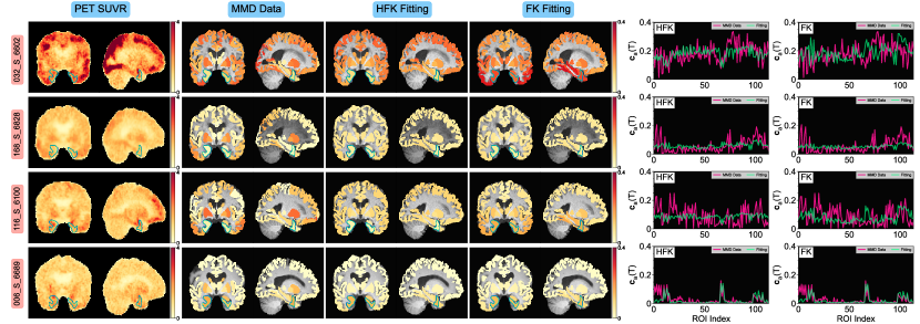
Figure 1: Reconstructions of four clinical patients with fixed IC. We assume the EC is the IC for all subjects here, and only try to estimate the scalar parameters. Each row stands for one clinical subject. From left to right in each panel, the figure shows SUVR image, processed regional tau abnormal MMD values (which is observation during the inversion), fitting from HFK model, fitting from FK model, 1D curve of fitting result from HFK model and FK model. The EC region is highlighted by solid contour line.

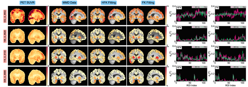
Figure 2: Reconstructions of four clinical patients. Instead of assuming EC as initial condition, we try to estimate the sparse IC from observation and assume the sparsity level of IC $s^{\text{max}}=5$. Each row stands for one clinical subject. From left to right in each panel, the figure shows PET image, processed regional tau abnormal MMD values (which is observation during the inversion), fitting from HFK model, fitting from FK model, 1D curve of fitting result from HFK model and FK model.

(CQ1) MMD advantage: We demonstrate that regional MMD features are a better indicator of tau abnormality than regional SUVR or tau positive probability in [10]. To accomplish this, we take 76 cognitively normal (CN) patients with age below 65 from the ADNI dataset and 45 patients with Alzheimer’s disease (AD). As for demographic, AD population has ages $74.96\pm 8.87$ and 19 are females, and 26 are males. CN patients are younger with ages $61.76\pm 3.71$ with 59 females and 17 males. For each patient, we extract regional SUVR, tau probability [10] and MMD scores. We explore three scenarios: we perform binary classification using a support vector machine (SVM) with a polynomial kernel, utilizing SUVR features. We repeat this classification using tau probability and MMD scores. The dataset is split into 60% training and 40% testing for reliable evaluation.

To select the most relevant features for classification, we rank the features based on their Pearson correlation score with the patient labels. We then classify the patients using a subset of the most highly correlated features. During the feature selection process, we incrementally add one additional feature each time and employ five-fold cross-validation to compute the mean and standard deviation of the classification accuracy on the training dataset. The optimal number of features is determined by selecting the subset with the highest mean-to-standard deviation ratio.

We use only four features from MMD, seven features from mean SUVR and twenty features from tau probability. We conduct the classification task and report the best-performing model for all three features in Table 3. The MMD approach achieved 97.9% accuracy on the test dataset compared to 89.4% accuracy using SUVR values and 91.5% using tau probability, highlighting its potential as a key feature for tau-PET data representation. Later we also show the superiority of MMD in inversion performance.

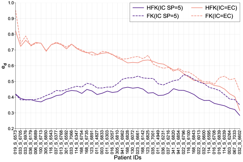
Figure 3: Inversion for 45 AD patients from ADNI dataset under HFK and FK models in two scenarios: IC=EC and IC(SP=5). The FK method with IC=EC is a popular model that people use to reconstruct the tau-PET data. We compare the methods regarding $e_{\mathbb{d}}$. The lines are moving average of relative errors across adjacent two patients. The patients are sorted by their summation of MMD concentration. The our inversion algorithm (IC (SP=5)) method with HFK model overall performs the best.

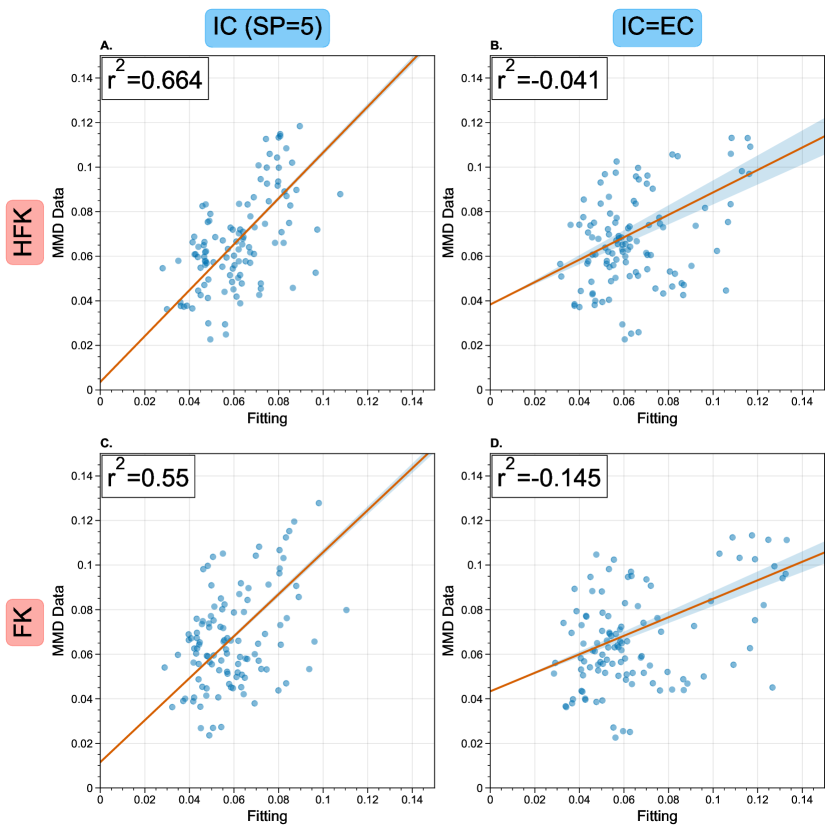
Figure 4: $r^{2}$ score for AD population using HFK and FK models with IC(SP=5) and IC=EC inversion methods. We compute the $r^{2}$ between averaged observation regional MMD and averaged fitting result for AD patients. Each dot represents average value at one parcel among all the population. We fit the dots by affine function and the blue shadow represents the three times standard deviation of fitted curve.

(CQ2) Models comparison: We conduct two experiments: firstly, we run inversion with HFK and FK models given that IC is located at EC (IC=EC) and only estimate the parameters $\kappa$, $\rho$, and $\gamma$. Second, we use our inversion algorithm for HFK and FK to estimate the parameters $\kappa$, $\rho$, $\gamma$ and $\mathbb{p}_{0}$. In the second experiment, as part of our inversion algorithm 2.2, we incorporate a sparsity hyper-parameter $s^{\text{max}}$. We select $s^{\text{max}}=5$ based on our tests, as the model’s performance does not significantly changes as we further increase this hyper-parameter. For the rest of the paper, we refer to the algorithm with IC inversion as IC(SP=5), while the inversion with a fixed IC at EC is denoted as IC=EC.

In Fig. 1 and Fig. 2, we plot the first and second scenarios, respectively, for four patients. We visualize the SUVR values for tau-PET scans, the parcellated tau MMD score (referred to as ”MMD data”), and the inversion results (Fitting) obtained using the FK and HFK models. We summarize the fitting performance for each patient in Table 4, where we report the $\ell_{2}$ relative error ($e_{\mathbf{d}}$) and $r^{2}$ values for both experiments. We report both mean and standard deviation as for the sensitivity evaluation of inversion regarding samples for each subject. For the case with IC=EC, in comparison to the FK model, the HFK model achieves upto 15.4% improvement in the $\ell_{2}$ norm relative error. In the case with IC(SP=5), HFK achieves a 27.3% relative error improvement (measured in $\ell_{2}$ norm) over the HFK model with IC=EC. Both FK and HFK models inverting IC outperform the cases with IC=EC, as they provide a greater degree of freedom in IC selection. The HFK model with IC(SP=5) exhibits the best overall performance.

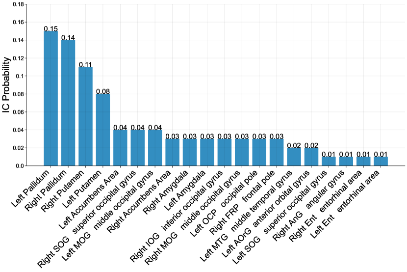
Figure 5: Probability of regions to be IC of AD. We pick the 20 mostly selected IC through our inversion for clinical AD patients. Under the presence of high variability in AD tau-PET data, EC is less likely to be chosen as the IC of disease propagation with probability 1%. The most common choice is Pallidum with probability as high as 15%.

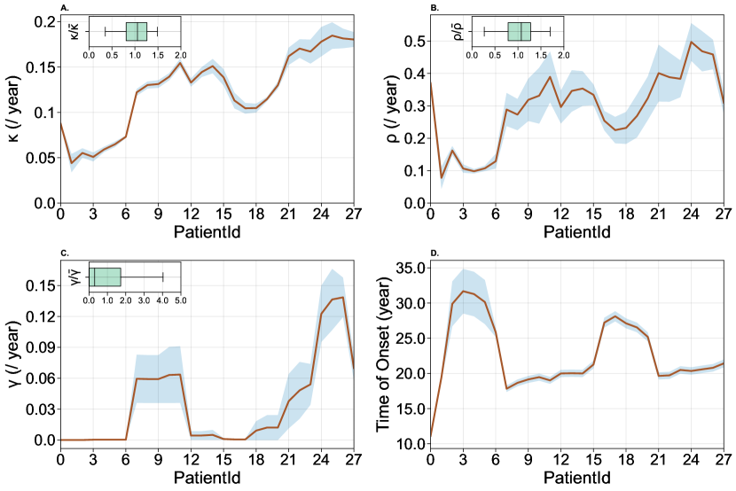
Figure 6: Longitudinal study of clinical patients. The line plot is the mean of the normalized values for each patient. The blue shadow represents the variability of normalized estimated parameters for each clinical patient. The results indicate the consistency of the inversion system. Box plot shown in the window of the subplots summarize the range of each parameter. Moreover, we plot the time of onset (in unit of ”year”). Most of these patients are estimated to have disease starting from 10–35 years ago before scans.

(CQ3) Performance on ADNI dataset: In this section, we evaluate the performance of the HFK and FK models on a cohort of 455 CN, 212 MCI and 45 AD patients from ADNI dataset. Here we mainly present results of AD patients for their heterogeneous tau distribution. We assess each model using the IC=EC and IC(SP=5) inversion algorithms.

In Fig. 3, we present the relative error $e_{\mathbf{d}}$ for each patient. The patients are ordered increasingly based on the level of tau abnormality ($\|\mathbf{d}\|_{1}$), and in nearly all AD patients, the HFK model with IC(SP=5) demonstrates superior performance. The HFK model achieves relative fitting errors as low as 28%. Notably, for patient 019_S_6573, IC(SP=5) achieves $\sim 40\%$ improvement w.r.t IC=EC for HFK model. Fig. 4 demonstrates the $r^{2}$ for two models and two inversion schemes. HFK model with IC inversion can explain 66.4% of the observation data, while the popular FK (EC) fails in the AD data fitting (with $r^{2}=-0.145$). We further test our scheme in 455 CN patients and achieves $r^{2}=0.8$, and 212 MCI patients with $r^{2}=0.729$, which validates the effectiveness of our method in different cognitive group. Furthermore, we tested tau positive probability [10] in our scheme. Tau probability achieves $r^{2}=0.5$ for AD patients under $s^{\text{max}}=10$ which shows the superior potential of MMD over tau probability.

We compute the frequency of IC locations chosen by our inversion scheme in Fig. 5. It indicates a preference for the Pallidum ($\sim 15\%$) and Putamen ($\sim 10\%$), while the Entorhinal Cortex (EC) are chosen only around 1%.

(CQ4) Clinical sensitivity analysis: To assess the sensitivity of the inversion scheme, we conduct experiments using different templates, parcellations, and connectivity matrices. For each patient, their T1 image is registered with five different template T1 images, resulting in variations in parcel size and location. Additionally, the T1 images reveal differences in grey matter and ventricle sizes across the brain. These variations directly impact the MMD score, as it depends on samples drawn from different regions. The inversion sensitivity regarding the five brain templates on AD patients is within 5% regarding $e_{\mathbb{d}}$.

To analyze the effects of parcellation on the model, we divide large regions into finer-grained regions via K-means to achieve a more uniform distribution of parcel volumes. There are around 450 parcels in the new parcellation (varies between templates). Under new parcellations, we calculate new MMD scores for all the templates we have. We run the inversion algorithm for the new parcellations. HFK model achieves an $r^{2}$ score of $0.584$ under the finer parcellation.

Our connectivity matrix is compared to the one derived from the widely used MRtrix3 software [46]. The inversion results are all done using HFK model with IC(SP=5) inversion method. Our connectivity matrix achieves better fitting relative error (40.97%) than MRtrix3 (45.18%). The inversion algorithm performs stable with different tractography methods.

(CQ5) Longitudinal Analysis: In cases where patients have undergone multiple tau-PET scans at distinct time points denoted as $t_{1}$ and $t_{2}$, we perform the inversion algorithm for each individual scan. Initially, we invert the model parameters ($\mathbf{p}_{0},\ \kappa,\rho,\gamma$) using either the direct inversion for $t_{1}$ or $t_{2}$. Subsequently, utilizing the estimated initial condition and parameters, we apply the HFK model to project the data forward or backward in time based on the temporal order of the scans (extrapolation or interpolation). The resulting projected model is then compared to the data from the second scan, and the projection time $\tau$ with the minimum error between the model prediction and the scan is determined.

By considering the time horizon $T$, $\tau$, and the real-life time gap between two scans, we are able to estimate the disease onset time. To facilitate a normalized comparison, we scale $\kappa,\ \rho,\ \gamma$ by dividing them with the estimated time of onset (expressed in years). In Fig. 6, we present the estimated parameters and time of onset. The line plot illustrates the mean parameter values, while the blue shadow shows standard deviation. Patients are ordered in increasing order based on their abnormality information ($\left\|\mathbf{d}\right\|_{1}$). The estimated parameters indicate that the majority of patients experience disease onset between 10 and 35 years after the initial symptoms.

We employed box plots to show the estimated normalized parameters as subplots in Fig. 6. The consistency of the estimated parameters and the plausible time of onset provides evidence that the model is capable of effective patient stratification. Considering the long term period of the disease progression, the results provide a promising application to do the early diagnosis.

4 Conclusion

We propose a novel inversion algorithm for a two-species HFK model exhibits improved qualitative consistency with tau-PET data compared to the existing FK model. Our model utilizes sparse initial conditions and three scalar parameters to represent migration, proliferation, and clearance. To estimate these parameters, we employ an inversion strategy that utilizes quasi-newton and compressive sampling method.

We validate our algorithm under synthetic scenario, and evaluate on ADNI dataset focusing on 45 AD patients. Based on several criteria, such as relative error and $r^{2}$, the HFK model with inverted initial conditions outperforms other methods overall using only a small number of parameters. To verify the stability and effectiveness of the model, we conduct sensitivity experiments with templates, parcellations, and connectivity matrices. Additionally, we analyze longitudinal data using our inversion algorithm. By incorporating patient-specific model parameters, we estimate the time of onset for AD. Our model suggests the existence of additional seeding locations apart from the entorhinal cortex (EC).

However, our current work has some limitations. We focus solely on tau lesion modeling and do not consider the influence of $A\beta$, which is recognized as an important factor in AD. Future research endeavors will integrate the effect of $A\beta$ into the tau modeling. From the perspective of the inversion, it will be interesting to add sparsity constraints to the connectivity matrix and make the connectivity as an additional optimization parameter.

References and Footnotes

References

- [1] L. Frontzkowski, M. Ewers, M. Brendel, D. Biel, R. Ossenkoppele, P. Hager, A. Steward, A. Dewenter, S. Römer, A. Rubinski et al., “Earlier alzheimer’s disease onset is associated with tau pathology in brain hub regions and facilitated tau spreading,” Nature Communications, vol. 13, no. 1, p. 4899, 2022.
- [2] Y. Blinkouskaya and J. Weickenmeier, “Brain shape changes associated with cerebral atrophy in healthy aging and alzheimer’s disease,” Frontiers in Mechanical Engineering, vol. 7, p. 705653, 2021.
- [3] N. Franzmeier, J. Neitzel, A. Rubinski, R. Smith, O. Strandberg, R. Ossenkoppele, O. Hansson, and M. Ewers, “Functional brain architecture is associated with the rate of tau accumulation in alzheimer’s disease,” Nature communications, vol. 11, no. 1, p. 347, 2020.
- [4] M. Yu, O. Sporns, and A. J. Saykin, “The human connectome in alzheimer disease—relationship to biomarkers and genetics,” Nature Reviews Neurology, vol. 17, no. 9, pp. 545–563, 2021.
- [5] T. E. Cope, T. Rittman, R. J. Borchert, P. S. Jones, D. Vatansever, K. Allinson, L. Passamonti, P. Vazquez Rodriguez, W. R. Bevan-Jones, J. T. O’Brien et al., “Tau burden and the functional connectome in alzheimer’s disease and progressive supranuclear palsy,” Brain, vol. 141, no. 2, pp. 550–567, 2018.
- [6] H. I. Jacobs, T. Hedden, A. P. Schultz, J. Sepulcre, R. D. Perea, R. E. Amariglio, K. V. Papp, D. M. Rentz, R. A. Sperling, and K. A. Johnson, “Structural tract alterations predict downstream tau accumulation in amyloid-positive older individuals,” Nature neuroscience, vol. 21, no. 3, pp. 424–431, 2018.
- [7] N. Franzmeier, A. Rubinski, J. Neitzel, Y. Kim, A. Damm, D. L. Na, H. J. Kim, C. H. Lyoo, H. Cho, S. Finsterwalder et al., “Functional connectivity associated with tau levels in ageing, alzheimer’s, and small vessel disease,” Brain, vol. 142, no. 4, pp. 1093–1107, 2019.
- [8] D. Biel, M. Brendel, A. Rubinski, K. Buerger, D. Janowitz, M. Dichgans, and N. Franzmeier, “Tau-pet and in vivo braak-staging as prognostic markers of future cognitive decline in cognitively normal to demented individuals,” Alzheimer’s research & therapy, vol. 13, no. 1, pp. 1–13, 2021.
- [9] K. A. Johnson, A. Schultz, R. A. Betensky, J. A. Becker, J. Sepulcre, D. Rentz, E. Mormino, J. Chhatwal, R. Amariglio, K. Papp et al., “Tau positron emission tomographic imaging in aging and early a lzheimer disease,” Annals of neurology, vol. 79, no. 1, pp. 110–119, 2016.
- [10] J. W. Vogel, Y. Iturria-Medina, O. T. Strandberg, R. Smith, E. Levitis, A. C. Evans, and O. Hansson, “Spread of pathological tau proteins through communicating neurons in human alzheimer’s disease,” Nature communications, vol. 11, no. 1, p. 2612, 2020.
- [11] S. Fornari, A. Schäfer, M. Jucker, A. Goriely, and E. Kuhl, “Prion-like spreading of alzheimer’s disease within the brain’s connectome,” Journal of the Royal Society Interface, vol. 16, no. 159, p. 20190356, 2019.
- [12] K. Scheufele, S. Subramanian, and G. Biros, “Calibration of biophysical models for tau-protein spreading in alzheimer’s disease from pet-mri,” arXiv preprint arXiv:2007.01236, 2020.
- [13] R. A. Fisher, “The wave of advance of advantageous genes,” Annals of eugenics, vol. 7, no. 4, pp. 355–369, 1937.
- [14] A. N. Kolmogorov, “A study of the equation of diffusion with increase in the quantity of matter, and its application to a biological problem,” Moscow University Bulletin of Mathematics, vol. 1, pp. 1–25, 1937.
- [15] S. L. DeVos, B. T. Corjuc, D. H. Oakley, C. K. Nobuhara, R. N. Bannon, A. Chase, C. Commins, J. A. Gonzalez, P. M. Dooley, M. P. Frosch et al., “Synaptic tau seeding precedes tau pathology in human alzheimer’s disease brain,” Frontiers in neuroscience, vol. 12, p. 267, 2018.
- [16] M. C. Hoenig, G. N. Bischof, J. Seemiller, J. Hammes, J. Kukolja, Ö. A. Onur, F. Jessen, K. Fliessbach, B. Neumaier, G. R. Fink et al., “Networks of tau distribution in alzheimer’s disease,” Brain, vol. 141, no. 2, pp. 568–581, 2018.
- [17] J. W. Vogel, A. L. Young, N. P. Oxtoby, R. Smith, R. Ossenkoppele, O. T. Strandberg, R. La Joie, L. M. Aksman, M. J. Grothe, Y. Iturria-Medina et al., “Four distinct trajectories of tau deposition identified in alzheimer’s disease,” Nature medicine, vol. 27, no. 5, pp. 871–881, 2021.
- [18] A. Gretton, K. M. Borgwardt, M. J. Rasch, B. Schölkopf, and A. Smola, “A kernel two-sample test,” The Journal of Machine Learning Research, vol. 13, no. 1, pp. 723–773, 2012.
- [19] A. Schäfer, J. Weickenmeier, and E. Kuhl, “The interplay of biochemical and biomechanical degeneration in alzheimer’s disease,” Computer methods in applied mechanics and engineering, vol. 352, pp. 369–388, 2019.
- [20] S. Subramanian, A. Ghafouri, K. M. Scheufele, N. Himthani, C. Davatzikos, and G. Biros, “Ensemble inversion for brain tumor growth models with mass effect,” IEEE Transactions on Medical Imaging, vol. 42, no. 4, pp. 982–995, 2022.
- [21] P. Vemuri, V. J. Lowe, D. S. Knopman, M. L. Senjem, B. J. Kemp, C. G. Schwarz, S. A. Przybelski, M. M. Machulda, R. C. Petersen, and C. R. Jack Jr, “Tau-pet uptake: regional variation in average suvr and impact of amyloid deposition,” Alzheimer’s & Dementia: Diagnosis, Assessment & Disease Monitoring, vol. 6, pp. 21–30, 2017.
- [22] A. Raj, “Graph models of pathology spread in alzheimer’s disease: an alternative to conventional graph theoretic analysis,” Brain connectivity, vol. 11, no. 10, pp. 799–814, 2021.
- [23] F. E. Cohen, K.-M. Pan, Z. Huang, M. Baldwin, R. J. Fletterick, and S. B. Prusiner, “Structural clues to prion replication,” Science, vol. 264, no. 5158, pp. 530–531, 1994.
- [24] J. T. Jarrett and P. T. Lansbury Jr, “Seeding “one-dimensional crystallization” of amyloid: a pathogenic mechanism in alzheimer’s disease and scrapie?” Cell, vol. 73, no. 6, pp. 1055–1058, 1993.
- [25] M. Bertsch, B. Franchi, N. Marcello, M. C. Tesi, and A. Tosin, “Alzheimer’s disease: a mathematical model for onset and progression,” Mathematical medicine and biology: a journal of the IMA, vol. 34, no. 2, pp. 193–214, 2017.
- [26] J. Weickenmeier, M. Jucker, A. Goriely, and E. Kuhl, “A physics-based model explains the prion-like features of neurodegeneration in alzheimer’s disease, parkinson’s disease, and amyotrophic lateral sclerosis,” Journal of the Mechanics and Physics of Solids, vol. 124, pp. 264–281, 2019.
- [27] Z. Wen, A. Ghafouri, and G. Biros, “A two-species model for abnormal tau dynamics in alzheimer’s disease,” in International Conference on Medical Image Computing and Computer-Assisted Intervention. Springer, 2023, pp. 69–79.
- [28] A. Schäfer, M. Peirlinck, K. Linka, E. Kuhl, and A. D. N. I. (ADNI), “Bayesian physics-based modeling of tau propagation in alzheimer’s disease,” Frontiers in physiology, vol. 12, p. 702975, 2021.
- [29] T. B. Thompson, P. Chaggar, E. Kuhl, A. Goriely, and A. D. N. Initiative, “Protein-protein interactions in neurodegenerative diseases: A conspiracy theory,” PLoS computational biology, vol. 16, no. 10, p. e1008267, 2020.
- [30] S. Pal and R. Melnik, “Nonlocal models in the analysis of brain neurodegenerative protein dynamics with application to alzheimer’s disease,” Scientific Reports, vol. 12, no. 1, p. 7328, 2022.
- [31] Y. Iturria-Medina, R. C. Sotero, P. J. Toussaint, A. C. Evans, and A. D. N. Initiative, “Epidemic spreading model to characterize misfolded proteins propagation in aging and associated neurodegenerative disorders,” PLoS computational biology, vol. 10, no. 11, p. e1003956, 2014.
- [32] D. Needell and J. A. Tropp, “Cosamp: Iterative signal recovery from incomplete and inaccurate samples,” Applied and computational harmonic analysis, vol. 26, no. 3, pp. 301–321, 2009.
- [33] S. Subramanian, K. Scheufele, M. Mehl, and G. Biros, “Where did the tumor start? an inverse solver with sparse localization for tumor growth models,” Inverse problems, vol. 36, no. 4, p. 045006, 2020.
- [34] K. Scheufele, S. Subramanian, and G. Biros, “Fully automatic calibration of tumor-growth models using a single mpmri scan,” IEEE transactions on medical imaging, vol. 40, no. 1, pp. 193–204, 2020.
- [35] H.-R. Kim, P. Lee, S. W. Seo, J. H. Roh, M. Oh, J. S. Oh, S. J. Oh, J. S. Kim, and Y. Jeong, “Comparison of amyloid and tau spread models in alzheimer’s disease,” Cerebral Cortex, vol. 29, no. 10, pp. 4291–4302, 2019.
- [36] D. Le Bihan, J.-F. Mangin, C. Poupon, C. A. Clark, S. Pappata, N. Molko, and H. Chabriat, “Diffusion tensor imaging: concepts and applications,” Journal of Magnetic Resonance Imaging: An Official Journal of the International Society for Magnetic Resonance in Medicine, vol. 13, no. 4, pp. 534–546, 2001.
- [37] A. Giese, L. Kluwe, B. Laube, H. Meissner, M. E. Berens, and M. Westphal, “Migration of human glioma cells on myelin,” Neurosurgery, vol. 38, no. 4, pp. 755–764, 1996.
- [38] F. R. Chung, Spectral graph theory. American Mathematical Soc., 1997, vol. 92.
- [39] C. Zhu, R. H. Byrd, P. Lu, and J. Nocedal, “Algorithm 778: L-bfgs-b: Fortran subroutines for large-scale bound-constrained optimization,” ACM Transactions on mathematical software (TOMS), vol. 23, no. 4, pp. 550–560, 1997.
- [40] J. A. Tropp and S. J. Wright, “Computational methods for sparse solution of linear inverse problems,” Proceedings of the IEEE, vol. 98, no. 6, pp. 948–958, 2010.
- [41] S. M. Smith, M. Jenkinson, M. W. Woolrich, C. F. Beckmann, T. E. Behrens, H. Johansen-Berg, P. R. Bannister, M. De Luca, I. Drobnjak, D. E. Flitney et al., “Advances in functional and structural mr image analysis and implementation as fsl,” Neuroimage, vol. 23, pp. S208–S219, 2004.
- [42] J. Doshi, G. Erus, Y. Ou, S. M. Resnick, R. C. Gur, R. E. Gur, T. D. Satterthwaite, S. Furth, C. Davatzikos, A. N. Initiative et al., “Muse: Multi-atlas region segmentation utilizing ensembles of registration algorithms and parameters, and locally optimal atlas selection,” Neuroimage, vol. 127, pp. 186–195, 2016.
- [43] B. B. Avants, N. Tustison, and G. Song, “Advanced normalization tools (ants),” Insight j, vol. 2, no. 365, pp. 1–35, 2009.
- [44] A. Dagley, M. LaPoint, W. Huijbers, T. Hedden, D. G. McLaren, J. P. Chatwal, K. V. Papp, R. E. Amariglio, D. Blacker, D. M. Rentz et al., “Harvard aging brain study: dataset and accessibility,” Neuroimage, vol. 144, pp. 255–258, 2017.
- [45] L. Petzold, “Automatic selection of methods for solving stiff and nonstiff systems of ordinary differential equations,” SIAM journal on scientific and statistical computing, vol. 4, no. 1, pp. 136–148, 1983.
- [46] J.-D. Tournier, R. Smith, D. Raffelt, R. Tabbara, T. Dhollander, M. Pietsch, D. Christiaens, B. Jeurissen, C.-H. Yeh, and A. Connelly, “Mrtrix3: A fast, flexible and open software framework for medical image processing and visualisation,” Neuroimage, vol. 202, p. 116137, 2019.