For Better or For Worse?
Learning Minimum Variance Features With Label Augmentation
Abstract
Data augmentation has been pivotal in successfully training deep learning models on classification tasks over the past decade. An important subclass of data augmentation techniques - which includes both label smoothing and Mixup - involves modifying not only the input data but also the input label during model training. In this work, we analyze the role played by the label augmentation aspect of such methods. We prove that linear models on linearly separable data trained with label augmentation learn only the minimum variance features in the data, while standard training (which includes weight decay) can learn higher variance features. An important consequence of our results is negative: label smoothing and Mixup can be less robust to adversarial perturbations of the training data when compared to standard training. We verify that our theory reflects practice via a range of experiments on synthetic data and image classification benchmarks.
1 Introduction
The training and fine-tuning procedures for current state-of-the-art (SOTA) computer vision models rely on a number of different data augmentation schemes applied in tandem (Yu et al., 2022; Wortsman et al., 2022; Dehghani et al., 2023). While some of these methods involve only transformations to the input training data - such as random crops and rotations (Cubuk et al., 2019) - a non-trivial subset of them also apply transformations to the input training label.
Perhaps the two most widely applied data augmentation methods in this subcategory are label smoothing (Szegedy et al., 2015) and Mixup (Zhang et al., 2018). Label smoothing replaces the one-hot encoded labels in the training data with smoothed out labels that assign non-zero probability to every possible class (see Section 2 for a formal definition). Mixup similarly smooths out the training labels, but does so via introducing random convex combinations of data points and their labels. As a result, Mixup modifies not only the training labels but also the training inputs. The general principles of label smoothing and Mixup have been extended to create several variants, such as Structural Label Smoothing (Li et al., 2020), Adaptive Label Smoothing (Wang et al., 2021), Manifold Mixup (Verma et al., 2019), CutMix (Yun et al., 2019), PuzzleMix (Kim et al., 2020), SaliencyMix (Uddin et al., 2020), AutoMix (Liu et al., 2021), and Noisy Feature Mixup (Lim et al., 2022).
Due to the success of label smoothing and Mixup-based approaches, an important question on the theoretical side has been understanding when and why these data augmentations improve model performance. Towards that end, several recent works have studied this problem from the perspectives of regularization (Guo et al., 2019; Carratino et al., 2020; Lukasik et al., 2020; Chidambaram et al., 2021), adversarial robustness (Zhang et al., 2020), calibration (Zhang et al., 2021; Chidambaram & Ge, 2023), feature learning (Chidambaram et al., 2023; Zou et al., 2023), and sample complexity (Oh & Yun, 2023).
Although the connection between the label smoothing and Mixup losses has been noted in both theory and practice (Carratino et al., 2020), there has not been (to the best of our knowledge) a unifying theoretical perspective on why the models trained using these losses exhibit similar behavior. In this paper, we aim to provide such a perspective by extending the ideas from previous feature learning analyses to the aspect shared in common between both Mixup and label smoothing: label augmentation. Our analysis allows us to identify a clear failure mode shared by both Mixup and label smoothing - that they can ignore higher variance features - which we also verify empirically.
1.1 Outline of Main Contributions
Our main contribution can be summarized as,
For linearly separable data distributions that can be learned using any one of multiple features, models trained with Mixup or label smoothing learn only the minimum variance feature.
In order to work up to this claim, we provide the necessary background on Mixup and label smoothing and formalize the notion of data distributions with multiple separating features in Section 2. Our definition draws heavily from the idea of multi-view data introduced by Allen-Zhu & Li (2021), but is considerably simpler as it does not involve patches or feature noise.
We then prove our main results in Section 3, where we show that linear models trained with Mixup or label smoothing on the aforementioned type of binary class data distribution are correlated only with the minimum variance feature in the data. On the other hand, we also show that linear models trained using just empirical risk minimization (ERM) and weight decay (so as to ensure a unique solution) have non-trivial correlation with the high variance feature in the data.
A key aspect of our analysis is that we can show a clear separation in terms of feature learning between Mixup/label smoothing and ERM in the setting of just linear models and linearly separable data distributions, whereas previous feature learning analyses of Mixup/similar (Chidambaram et al., 2023; Zou et al., 2023) have relied on data distributions that are explicitly constructed to not be learnable by linear models and have an asymptotically large number of classes. As a result, our analysis is both simpler than existing analyses and shows that nonlinear training dynamics are not necessary to separate Mixup/label smoothing and ERM with respect to feature learning.
We also verify that our theoretical results extend to practice across several experimental settings. In Section 4.1, we show that for synthetic data following our theoretical assumptions, logistic regression trained with Mixup or label smoothing learns a weight vector that is effectively uncorrelated with the high variance feature in the data. We also show that this behavior extends beyond synthetic data in Section 4.2, where we train logistic regression models on binary classification versions of CIFAR-10 and CIFAR-100 modified to have adversarial pixels in the training data that completely identify each class. In this case, the Mixup and label smoothing logistic regression models do not generalize at all due to having learned only the adversarial pixels in the training data.
Finally, we show in Section 4.3 that these observations still apply even when we consider ResNets trained on the full versions of CIFAR-10 and CIFAR-100; for these experiments we follow the experimental setup introduced by Chidambaram et al. (2023) in which the training data is modified to have extra low variance features via additional channels. Our results provide a contrasting perspective to that of Chidambaram et al. (2023) - Mixup (and label smoothing) can end up learning only the low variance features in the training data, whereas ERM can avoid this problem.
1.2 Related Work
Label Smoothing. Since being introduced by Szegedy et al. (2015), label smoothing continues to be used to train SOTA vision (Wortsman et al., 2022; Liu et al., 2022), translation (Vaswani et al., 2017; Team et al., 2022), and multi-modal models (Yu et al., 2022). Attempts to understand when and why label smoothing is effective can be traced back to the influential empirical analyses of Pereyra et al. (2017) and Müller et al. (2020), which respectively relate label smoothing to entropy regularization and show that it can lead to more closely clustered learned representations, with the latter work further showing that these clustered representations can be responsible for decreased distillation performance.
On the theoretical side, Lukasik et al. (2020) study the relationship between label smoothing and loss correction techniques used to handle label noise, and show that label smoothing can be effective for mitigating label noise. Liu (2021) extends this line of work by analyzing how label smoothing can outperform loss correction in the context of memorization of noisy labels. Wei et al. (2022) further show that negative label smoothing can outperform traditional label smoothing in the presence of label noise. Xu et al. (2020) provide an alternative theoretical perspective, showing that label smoothing can improve convergence of stochastic gradient descent. However, to the best of our knowledge, there are no preexisting theoretical works attempting to understand how label smoothing affects feature learning.
Mixup. Similar to label smoothing, Mixup (Zhang et al., 2018) and its aforementioned variants have also played an important role in the training of SOTA vision (Wortsman et al., 2022; Liu et al., 2022), text classification (Sun et al., 2020), translation (Li et al., 2021), and multi-modal models (Hao et al., 2023), often being applied alongside label smoothing. Initial work on understanding Mixup studied it from the perspective of introducing a data-dependent regularization term to the empirical risk (Carratino et al., 2020; Zhang et al., 2020; Park et al., 2022), with Zhang et al. (2020) and Park et al. (2022) showing that this regularization effect can lead to improved Rademacher complexity.
On the other hand, Guo et al. (2019) and Chidambaram et al. (2021) show that the regularization terms introduced by the Mixup loss can also have a negative impact due to the fact that Mixup-augmented points may coincide with existing training data points, leading to models that fail to minimize the original risk. Mixup has also been studied from the perspective of calibration (Thulasidasan et al., 2019), with theoretical results (Zhang et al., 2021; Chidambaram & Ge, 2023) showing that Mixup training can prevent miscalibration issues arising from ERM (even when post-training calibration methods are used with ERM).
Very recently, Oh & Yun (2023) studied Mixup in a similar context to our work (binary classification with linear models), and showed that Mixup can significantly improve the sample complexity required to learn the optimal classifier when compared to ERM. Also recently, and most closely related with our results in this paper, Mixup has been studied from a feature learning perspective, with Chidambaram et al. (2023) and Zou et al. (2023) both showing that Mixup training can learn multiple features in a generative, multi-view (Allen-Zhu & Li, 2021) data model despite ERM failing to do so. We provide a more detailed comparison to these works when we discuss our main results in Section 3.
General Data Augmentation. General data augmentation techniques have been a mainstay in image classification since the rise of deep learning models for such tasks (Krizhevsky et al., 2012). As a result, there is an ever-growing body of theory (Bishop, 1995; Dao et al., 2019; Wu et al., 2020; Hanin & Sun, 2021; Rajput et al., 2019; Yang et al., 2022; Wang et al., 2022; Chen et al., 2020; Mei et al., 2021) aimed at addressing broad classes of augmentations such as those resulting from group actions (i.e. rotations and reflections). Recently, Shen et al. (2022) also studied a class of linear data augmentations from a feature learning perspective, once again using a data model based on the multi-view data of Allen-Zhu & Li (2021). This work is in the same vein as that of Zou et al. (2023) and Chidambaram & Ge (2023), although the augmentation considered is not comparable to Mixup.
2 Preliminaries
Notation. Given , we use to denote the set . For a vector and a subset , we use to denote the restriction of to only those indices in , and also use to denote the coordinate of . The same notation also applies to matrices; i.e. for a matrix we use to denote the restriction of the rows of to only those dimensions in . Additionally, we use to denote the partial order over positive definite matrices and to denote the identity matrix. We use to indicate the Euclidean norm on . For two sets of points we use to denote the distance between and . For a function we use to denote the coordinate function of . For a probability distribution we use to denote its support. Additionally, if corresponds to the joint distribution of two random variables and (i.e. data and label), we use and to denote the respective marginals, and and to denote the conditional distributions.
Our theory will focus on binary classification problems in in which a subset of the input dimensions correspond to a low variance feature, and the complementary dimensions correspond to a higher variance but more separable feature. This setup is intended to mimic standard explorations of robustness of image classification models. For example, if each class in the data has a small set of constant, identifying pixels in every training point (either introduced adversarially or as an artifact of the domain being considered), does a model trained on this data learn to predict using only the identifying pixels or the whole image?
The goal in such cases is typically to also learn the features present in the non-identifying pixels (i.e. the higher variance features). We will show, however, that doing any kind of label augmentation (label smoothing or Mixup) in this low variance/high variance feature setup will lead to learning a model that has only learned the low variance feature, while standard training will lead to having non-trivial correlation with the high variance feature.
It is also natural to ask whether this phenomenon is purely a result of the fact that augmented labels (i.e. not 0 or 1) prevent the learned model weights from going to infinity, which has been pointed out to be crucial in previous existing analyses of Mixup (Chidambaram et al., 2023). We answer this question in the negative by also showing that training using ERM with weight decay still learns the high variance feature in the data, so the variance minimization effect is more than just a weight norm constraint.
2.1 Data Model
We begin with the generative model of the data that we will work with. For simplicity, we consider the low variance feature to have zero variance conditional on the label - it is not difficult to extend our results to the case where the variance of this feature is simply much less than that of the high variance feature, but considering zero conditional variance yields cleaner proofs. We also consider balanced classes to further simplify the proofs, but our results will hold so long as each class appears with some non-zero probability.
Definition 2.1.
[Data Distribution] Let and be the sets denoting the low variance feature and high variance feature in the data respectively. We define to be any distribution on with and for both , along with the following properties:
-
1.
(Zero Conditional Variance in ) For -a.e. , we have that there exists a such that with .
-
2.
(Non-zero Conditional Variance in ) Let and , then (the restriction of to ) is positive definite.
-
3.
(More Separable High Variance Feature) Let . Then are compact, convex, and disjoint and satisfy .
Since Definition 2.1 corresponds to a linearly separable data distribution, we can restrict our attention to linear models of the form , where is the sigmoid function. We can then define the binary cross-entropy with weight decay as:
| (2.1) |
With thereby indicating the regular binary cross-entropy without weight decay. In what follows, we will work with the population form of the loss as defined in Equation (2.1), since for we have that is strictly convex and therefore we may simply analyze its unique minimizer as opposed to worrying about training dynamics.
Although will not have a unique minimizer, our results will still apply to the common case where is minimized by scaling the max-margin solution, which we define below.
Definition 2.2.
[Max-Margin Solution] The max-margin solution with respect to is defined to be:
| (2.2) |
2.2 Label Smoothing
Label smoothing as introduced by Szegedy et al. (2015) is intended to work with multi-class classification problems in which the data distribution is typically defined on . In this case, we work with models (the probability simplex in ), and the cross-entropy loss is simply .
The label-smoothed cross-entropy is then obtained by replacing the one-hot encoded label with a mixture of the original label and the uniform distribution over . Namely, the label-smoothed loss with mixing hyperparameter is defined to be:
| (2.3) |
For the purposes of our theory, however, we will be working with models of the form and labels , so we will consider the binary label-smoothed loss defined as:
| (2.4) |
Note that similar to Equation (2.1) the latter is defined as a function of the weight vector instead of the full model .
2.3 Mixup
Similar to label smoothing, Mixup (Zhang et al., 2018) was also introduced in the context of multi-class classification. In addition to augmenting the one-hot encoded labels , Mixup also augments the input data by combining both with another data point via a random convex combination. Both of these transformations are done according to a mixing distribution (which is a hyperparameter) whose support is contained in . To simplify notation, we will use and to denote multiple data points and their corresponding labels . Additionally, in the multi-class setting with , we also define:
| (2.5) | ||||
| (2.6) |
We may then define the Mixup cross-entropy:
| (2.7) |
Where is shorthand for . As before, since our theory focuses on binary classification and linear models , we may identically define the binary version of Equation (2.7) except for redefining to be:
| (2.8) |
Again, observe that we have redefined to directly be a function of instead of .
3 Main Theoretical Results
Having established the necessary background, we now state our main results. Full proofs of all results can be found in Appendix A. We first show that the unique minimizer of the standard risk with weight decay (as defined in Equation (2.1)) has non-trivial correlation with the high variance dimensions of the input .
Theorem 3.1.
Let be the unique minimizer of for . Then . In other words, the optimal solution under weight decay has significant weight in the high variance dimensions .
Proof Sketch. We can orthogonally decompose the optimal solution in terms of the unit normal max-margin directions and separating and respectively. Then, using the fact that for all (from assumption three in Definition 2.1), we can claim that must have greater weight associated with than , as otherwise we can decrease by moving some weight from to .
We cannot immediately extend the result of Theorem 3.1 to the binary cross-entropy without weight decay, since there is no unique minimizer of . However, for linear models trained with gradient descent (as is often done in practice), it is well-known that the learned model converges in direction to the max-margin solution (Soudry et al., 2018; Ji & Telgarsky, 2020). For this case, the proof technique of Theorem 3.1 readily extends and we obtain the following corollary.
Corollary 3.2.
If is the max-margin solution to , then the result of Theorem 3.1 still holds.
On the other hand, as alluded to earlier, this phenomenon does not occur when considering the label smoothing and Mixup losses and . Indeed, we can show:
Theorem 3.3.
Every minimizer of for satisfies , so the optimal solutions under label smoothing have no weight in the high variance dimensions.
Proof Sketch. The optimal prediction at a label-smoothed point is either or (depending on whether the label is or respectively). We can thus construct a predictor that is optimal at every point by choosing to have the appropriate correlation with and having no correlation with . That there are no equally good predictors that have correlation with can be shown by appealing to convexity.
Analogously, we have the following result for Mixup:
Theorem 3.4.
Every minimizer of satisfies for any distribution with that is not a point mass on either 0 or 1.
Proof Sketch. The proof setup is similar to that of Theorem 3.3, i.e. we try to find a stationary point of that is zero in the high variance dimensions. The difficulty in the Mixup analysis is that it is not possible to directly construct a point-wise optimal predictor like in the proof of Theorem 3.3 due to the different possibilities for mixed points (and mixed labels), and consequently there is no obvious construction for a stationary point. However, we can analyze the limiting behavior of the Mixup gradient with respect to the weight correlation with the low variance dimensions and still show that such a stationary point must exist.
Comparisons to existing results. We are not aware of any existing results on feature learning for label smoothing; prior theoretical work largely focuses on the relationship between label smoothing and learning under label noise, which is orthogonal to the perspective we take in this paper. Although feature learning results exist for Mixup (Chidambaram et al., 2023; Zou et al., 2023), the pre-existing results are constrained to the case of mixing using point mass distributions and only prove a separation between Mixup and unregularized ERM, whereas our results work for arbitrary mixing distributions (that don’t coincide with ERM) and also separate Mixup from ERM with weight decay. This greater generality comes at the cost of considering only linear models and linearly separable data, however, as both Chidambaram et al. (2023) and Zou et al. (2023) consider non-linearly separable data and the training dynamics of 2-layer neural networks.
Additionally, our results can be viewed as generalizing the observations made by Chidambaram et al. (2023), which were that Mixup can learn multiple features in the data when doing so decreases the variance of the learned predictor. In our case, we directly show that Mixup will learn the low variance feature in the data as opposed to the high variance feature. Our results also do not contradict the observations of Zou et al. (2023), which were that Mixup can learn both a “common” feature and a “rare” feature in the data; in their setup the common/rare features are fixed (zero variance) per class and concatenated with high variance noise.
4 Experiments

We now verify the predictions of our theoretical results in Section 3 across a variety of experimental setups. All experiments in this section were conducted on a single P100 GPU using PyTorch (Paszke et al., 2019) for model implementation. All reported results correspond to means over 5 training runs, and shaded regions in the figures correspond to 1 standard deviation bounds.
4.1 Synthetic Data
We first consider the case of training logistic regression models on a synthetic data distribution that exactly follows the assumptions of Definition 2.1.
Definition 4.1 (Synthetic Data).
We define a distribution parameterized by (where ) on with and satisfying:
-
1.
First dimensions are constant but small. We have for .
-
2.
Last dimensions are high variance. We have for .
In other words, we consider data where (conditional on the label) the first half of the dimensions are fixed (corresponding to ) and the second half are i.i.d. high variance uniform (corresponding to ). We sample data points according to Definition 4.1 with and and train logistic regression models across a range of settings for weight decay, label smoothing, and Mixup.111The choice of here and throughout the rest of this section is relatively arbitrary; we verified that our experimental phenomena are unchanged for other scales such as .
Namely, we consider 20 uniformly spaced values in for the weight decay parameter and in for the label smoothing parameter, where the upper bound for the label smoothing parameter space is obtained from the experiments of Müller et al. (2020). For Mixup, we fix the mixing distribution to be the canonical choice of introduced by Zhang et al. (2018) and consider 20 uniformly spaced values in (with corresponding to ERM), which effectively covers the range of Mixup hyperparameter values used in practice.
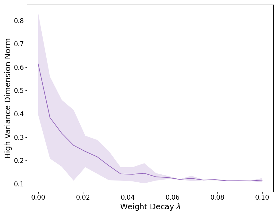
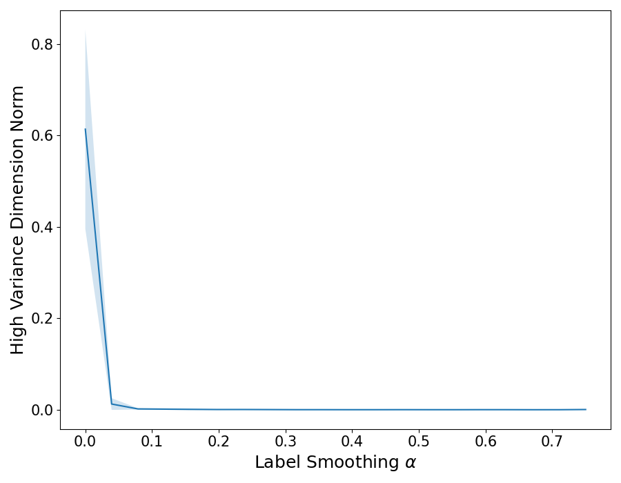
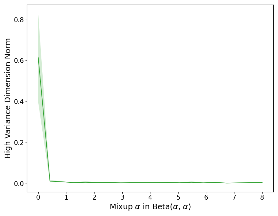
We train all models for 100 epochs using Adam with the standard hyperparameters of , a learning rate of , and a batch size of 500. At the end of training, we compute (i.e. the norm of the weight vector in the last 5 dimensions) for each trained model. For each model setting, we report the mean and standard deviation of over 5 training runs in Figure 1.
As can be seen from the results, the weight decay models always have non-trivial values for (even for large values of ), whereas the label smoothing and Mixup models very quickly converge to a of effectively zero as their respective hyperparameters move away from the ERM regime ( in both cases). This matches the behavior predicted by Theorems 3.1 to 3.4.
It is natural to ask to what extent these results depend on the fact that the low variance features in Definition 4.1 (the first half of the dimensions) actually have zero variance conditional on the label. As we mentioned in our theoretical results, it is sufficient to assume that the variance of the dimensions in is simply much less than that of , and the fact that we consider zero variance is merely for simplifying purposes. We verify that this is true in practice by re-running the above experiments but modifying the dimensions in to have non-zero variance by adding uniformly distributed noise on the scale of . The results remain unchanged; the corresponding plots can be found in Section B of the Appendix.
4.2 Binary Image Classification
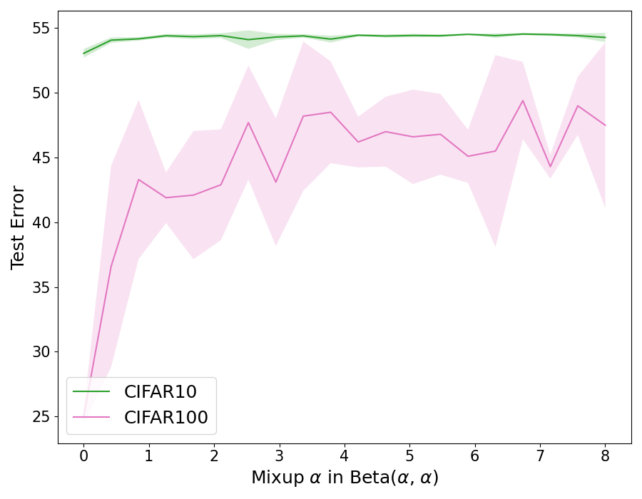
Although the experiments of Section 4.1 constitute a direct verification of our theory, in practice the low and high variance features are typically not as obviously partitioned as in Definition 4.1 and the metric we care about is usually generalization error as opposed to the strength of correlation with some part of the data. As such, we now relax our strict adherence to the assumptions of Definition 2.1 and consider binary classification on image data.
To do so, we reduce the standard benchmarks of CIFAR-10 and CIFAR-100 (Krizhevsky, 2009) to binary classification tasks by maintaining only the first two classes (“airplane” and “automobile” for CIFAR-10, “apple” and “aquarium fish” for CIFAR-100) and assigning them the labels of -1 and 1 respectively. This leads to 10000 training examples and 2000 test examples in the case of CIFAR-10, and 1000 training examples and 200 test examples in the case of CIFAR-100.
We preprocess the training data to have mean zero and variance one along every image channel (and apply the same transform to the test data), and then modify the training data such that the top left value (corresponding to the “R” channel of the top left pixel in the original image) in the tensor representation of the training input is replaced by , where as in Section 4.1. This ensures that the training data is separable in the first dimension of the data, although unlike in the case of Definition 4.1 we make no modifications to the other dimensions of the data to ensure separability outside the first dimension. We leave the test data unchanged - our goal is to determine whether models trained on the modified training data can learn more than just the single identifying dimension.
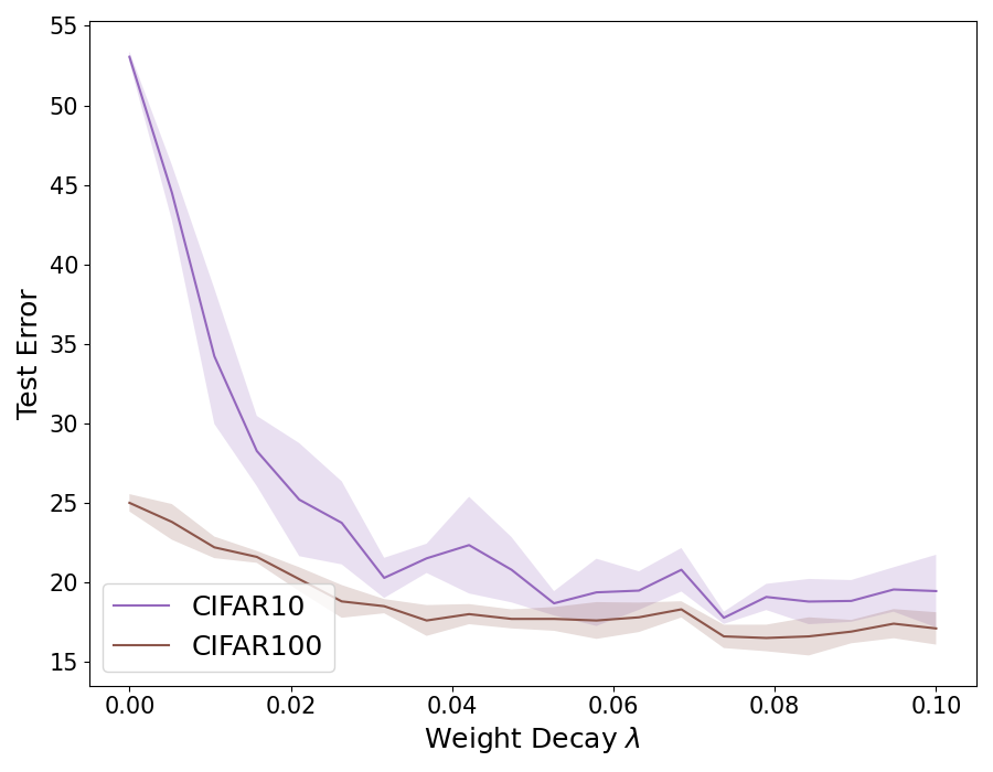
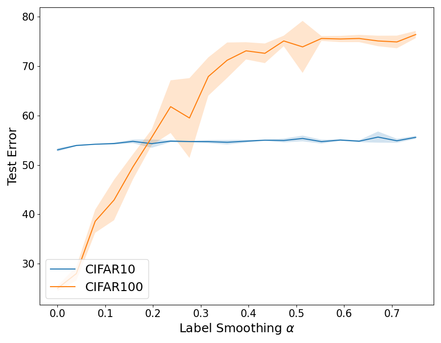
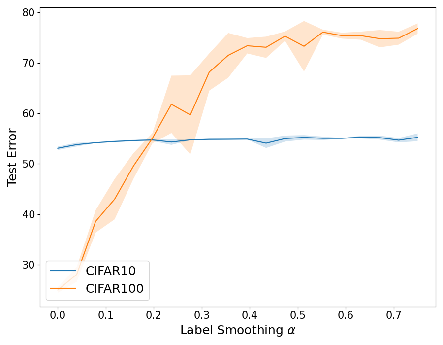
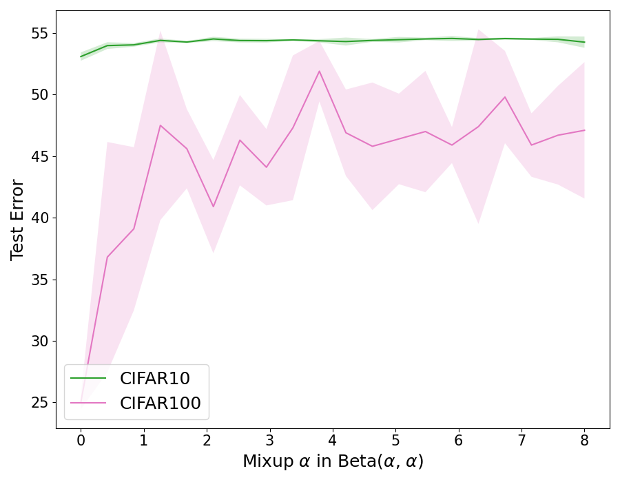
We follow the exact same logistic regression training setup as in Section 4.1, and sweep over the same hyperparameter values for weight decay, label smoothing, and Mixup. We report the mean test error along with one standard deviation error bounds over five training runs for each model setting in Figure 2.
The results mirror our observations in Section 4.1: both the label smoothing and Mixup models have high test error for all settings (in this case, ERM performs poorly as well) while weight decay achieves a significantly lower test error for all . The higher variance in the reported CIFAR-100 test errors can almost certainly be attributed to the fact that our binary version of CIFAR-100 consists of only 1000 training points and 200 points.
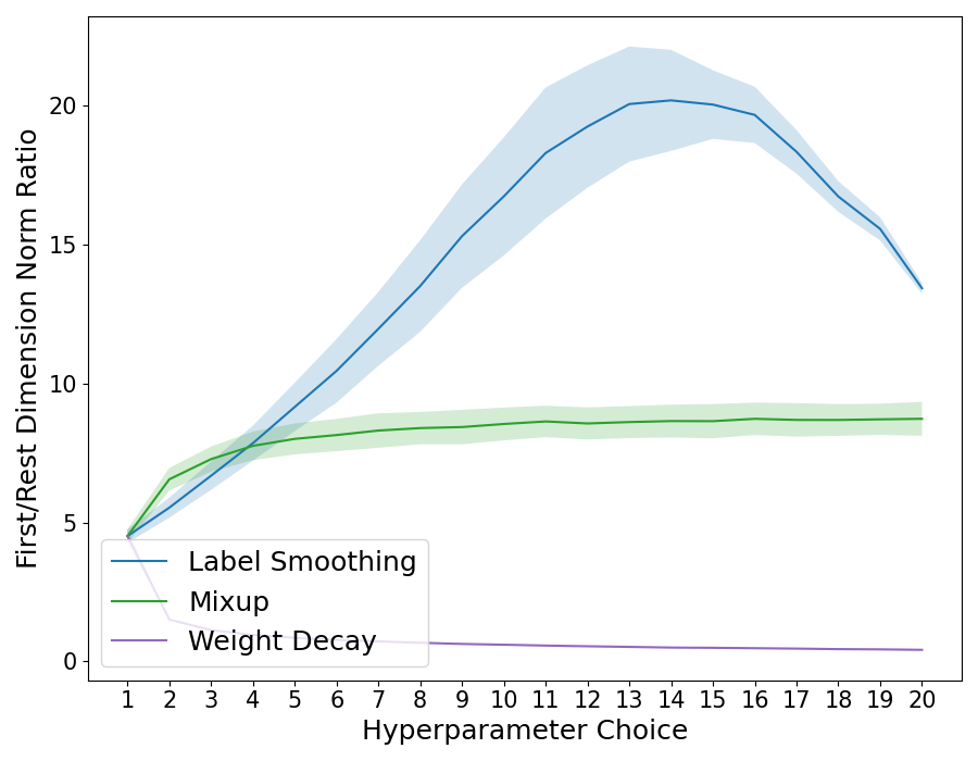
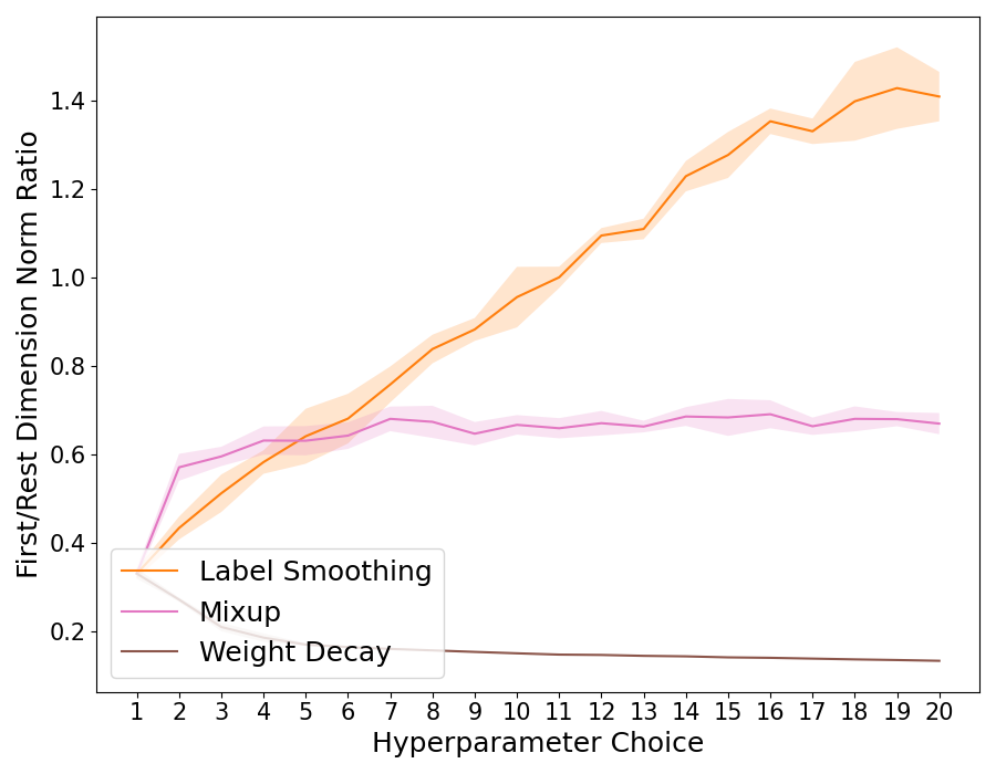
Our results correspond once again to label smoothing and Mixup learning to use only the zero variance, identifying dimension of the input, as we expect from our theory. Indeed, we verify this in Figure 3 where we plot the ratio (i.e. the ratio between the norm of the trained model weight vector in the first dimension and the remaining dimensions). We observe that for both CIFAR-10 and CIFAR-100, across all the non-ERM hyperparameter settings (refer to Section 4.1 for the range of hyperparameters) that both label smoothing and Mixup place much greater weight in the first dimension than weight decay.
As with the experiments of Section 4.1, we again check that the results here do not rely on the fact that the identifying dimension introduced into the training data has zero variance conditional on the label. As before, introducing uniformly distributed noise on the scale of to the identifying dimension does not change our results, and the corresponding plots can again be found in Section B of the Appendix.
4.3 Multi-Class Image Classification
Thus far we have considered training logistic regression models to stay within the confines of our theory, but we now investigate whether our observations extend to the more practical setting of training nonlinear models (i.e. deep neural networks) on multi-class image classification data.
As in Section 4.2, we consider CIFAR-10 and CIFAR-100, but this time maintain all of the original classes in both datasets. We once again preprocess the training data to have mean zero and variance one, and apply this transform to the test data as well. Unfortunately, unlike in Section 4.2, introducing a zero variance, identifying feature into each class in the training data would now require modifying a more significant portion of each image (for example, a patch for CIFAR-100 to identify each class).
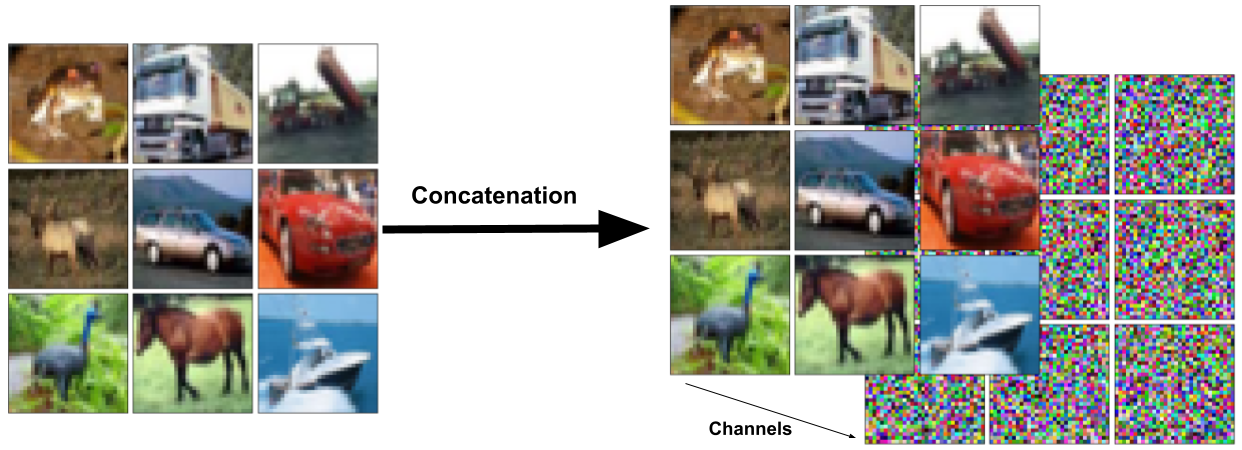
So as to preserve most of the original image content, as well as to have a more direct comparison to prior work, we choose to adopt a similar experimental setup to that of Chidambaram et al. (2023). Namely, we assign a random vector sampled from (where is the dimension of the data) to each class and concatenate this class vector along the channels dimension to every training data point for that class. A visualization of this transformation is shown in Figure 5. For the test data points, we concatenate an all-zero vector of the same size so as to preserve the dimensionality across train and test, as was done by Chidambaram et al. (2023). We take , so as to account for the dimensionality of the concatenated feature.
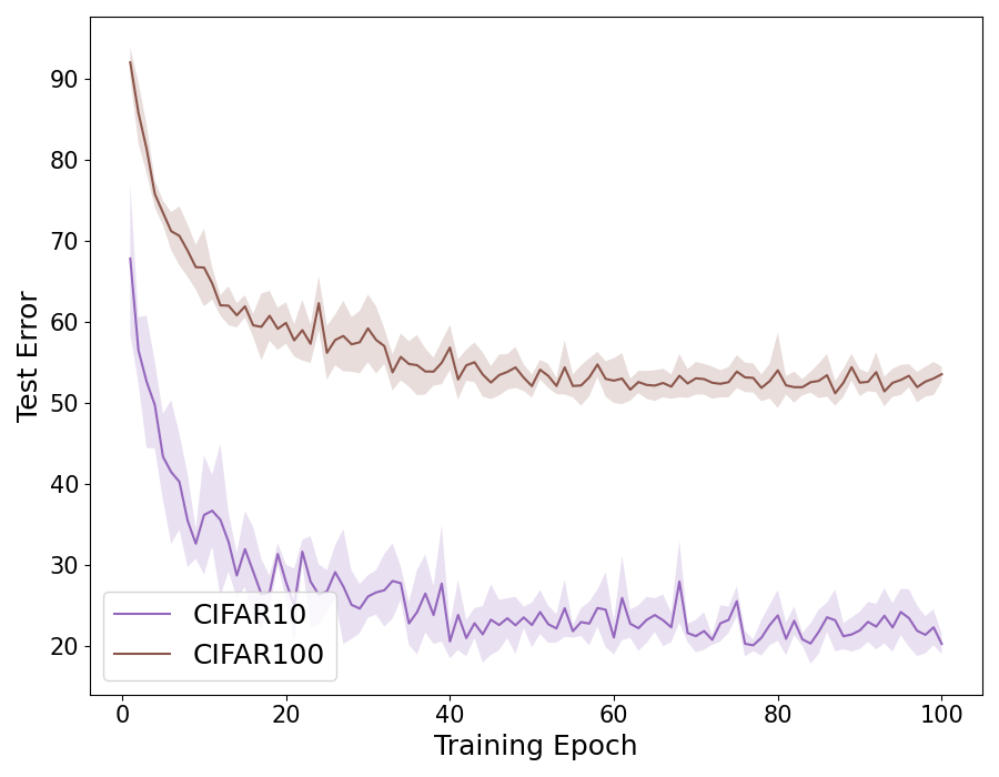
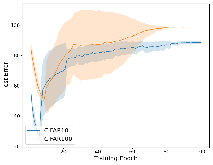
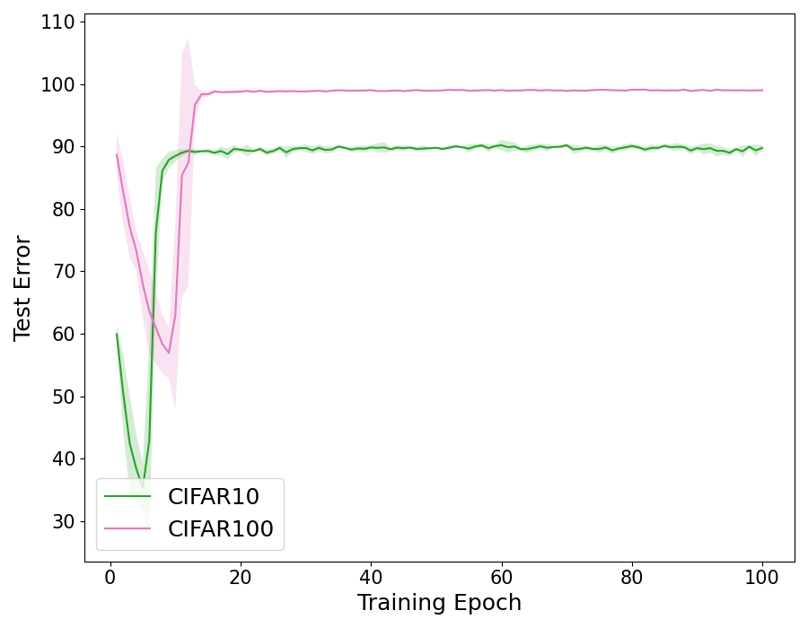
For both datasets, we train ResNet-18 models (He et al., 2015) for 100 epochs using Adam with the standard hyperparameters of , a learning rate of , and a batch size of 500. Due to the higher compute cost of training these models compared to the logistic regression models of Sections 4.1 and 4.2, we do not perform a full hyperparameter sweep but instead use known well-performing settings for weight decay, label smoothing, and Mixup. Namely, we use for weight decay, for label smoothing (Müller et al., 2020), and in for Mixup (Zhang et al., 2018). Since we are now dealing with nonconvex training dynamics, we report the mean test error over five runs at the end of each epoch with one standard deviation error bounds for each model setting in Figure 4.
As can be seen from the plots, both label smoothing and Mixup initially decrease the test error in the initial stages of training, but then overfit to the concatenated zero variance features. On the other hand, the test error for weight decay decreases over the course of training until effectively converging. This once again does not contradict what was observed by Chidambaram et al. (2023), as in their case their concatenated features were weighted alongside with the original image data so that variance could be decreased by learning both.
We also considered the case of low variance concatenated features as opposed to zero variance concatenated features in the training data. Similar to the results of Sections 4.1 and 4.2, the label smoothing and Mixup overfitting phenomenons persist even when we introduce variance to the concatenated features. However, we found that unless the introduced variance is much smaller (i.e. multiple orders of magnitude) than the concatenated feature scale , weight decay also overfits to the concatenated features. This brittleness is possibly an artifact of the chosen experimental setup and/or hyperparameters, but due to compute constraints we did not exhaustively explore this behavior and instead leave it as an open direction for follow-up work extending our results to non-linear/non-convex settings.
5 Conclusion
In summary, we have shown that for linearly separable data distributions in which there exist high variance features and much lower variance features, linear models trained with the data augmentation schemes of label smoothing and Mixup fail to learn the low variance features in both practice and theory, while standard training with weight decay succeeds. The main practical takeaway from this is that label smoothing and Mixup do not necessarily always improve the robustness of models, and their failure to do so may be indicative of certain identifying features in the training data (i.e. adversarially introduced patches). A natural follow-up to the results we have presented is an extension to the case of non-linear models and non-linearly-separable data, which the results of Section 4.3 indicate should be possible.
Acknowledgements
Rong Ge and Muthu Chidambaram are supported by NSF Award DMS-2031849 and CCF-1845171 (CAREER). Muthu would like to thank Annie Tang for thoughtful feedback during the early stages of this project.
References
- Allen-Zhu & Li (2021) Allen-Zhu, Z. and Li, Y. Towards understanding ensemble, knowledge distillation and self-distillation in deep learning, 2021.
- Bishop (1995) Bishop, C. M. Training with noise is equivalent to tikhonov regularization. Neural computation, 7(1):108–116, 1995.
- Carratino et al. (2020) Carratino, L., Cissé, M., Jenatton, R., and Vert, J.-P. On mixup regularization, 2020.
- Chen et al. (2020) Chen, S., Dobriban, E., and Lee, J. A group-theoretic framework for data augmentation. Advances in Neural Information Processing Systems, 33:21321–21333, 2020.
- Chidambaram & Ge (2023) Chidambaram, M. and Ge, R. On the limitations of temperature scaling for distributions with overlaps, 2023.
- Chidambaram et al. (2021) Chidambaram, M., Wang, X., Hu, Y., Wu, C., and Ge, R. Towards understanding the data dependency of mixup-style training. CoRR, abs/2110.07647, 2021. URL https://arxiv.org/abs/2110.07647.
- Chidambaram et al. (2023) Chidambaram, M., Wang, X., Wu, C., and Ge, R. Provably learning diverse features in multi-view data with midpoint mixup. In Krause, A., Brunskill, E., Cho, K., Engelhardt, B., Sabato, S., and Scarlett, J. (eds.), International Conference on Machine Learning, ICML 2023, 23-29 July 2023, Honolulu, Hawaii, USA, volume 202 of Proceedings of Machine Learning Research, pp. 5563–5599. PMLR, 2023. URL https://proceedings.mlr.press/v202/chidambaram23a.html.
- Cubuk et al. (2019) Cubuk, E. D., Zoph, B., Shlens, J., and Le, Q. V. Randaugment: Practical automated data augmentation with a reduced search space, 2019.
- Dao et al. (2019) Dao, T., Gu, A., Ratner, A., Smith, V., De Sa, C., and Ré, C. A kernel theory of modern data augmentation. In International Conference on Machine Learning, pp. 1528–1537. PMLR, 2019.
- Dehghani et al. (2023) Dehghani, M., Djolonga, J., Mustafa, B., Padlewski, P., Heek, J., Gilmer, J., Steiner, A., Caron, M., Geirhos, R., Alabdulmohsin, I., Jenatton, R., Beyer, L., Tschannen, M., Arnab, A., Wang, X., Riquelme, C., Minderer, M., Puigcerver, J., Evci, U., Kumar, M., van Steenkiste, S., Elsayed, G. F., Mahendran, A., Yu, F., Oliver, A., Huot, F., Bastings, J., Collier, M. P., Gritsenko, A., Birodkar, V., Vasconcelos, C., Tay, Y., Mensink, T., Kolesnikov, A., Pavetić, F., Tran, D., Kipf, T., Lučić, M., Zhai, X., Keysers, D., Harmsen, J., and Houlsby, N. Scaling vision transformers to 22 billion parameters, 2023.
- Guo et al. (2019) Guo, H., Mao, Y., and Zhang, R. Mixup as locally linear out-of-manifold regularization. In Proceedings of the AAAI Conference on Artificial Intelligence, volume 33, pp. 3714–3722, 2019.
- Hanin & Sun (2021) Hanin, B. and Sun, Y. How data augmentation affects optimization for linear regression. Advances in Neural Information Processing Systems, 34, 2021.
- Hao et al. (2023) Hao, X., Zhu, Y., Appalaraju, S., Zhang, A., Zhang, W., Li, B., and Li, M. Mixgen: A new multi-modal data augmentation, 2023.
- He et al. (2015) He, K., Zhang, X., Ren, S., and Sun, J. Deep residual learning for image recognition. CoRR, abs/1512.03385, 2015. URL http://arxiv.org/abs/1512.03385.
- Ji & Telgarsky (2020) Ji, Z. and Telgarsky, M. Characterizing the implicit bias via a primal-dual analysis, 2020.
- Kim et al. (2020) Kim, J.-H., Choo, W., and Song, H. O. Puzzle mix: Exploiting saliency and local statistics for optimal mixup. In International Conference on Machine Learning, pp. 5275–5285. PMLR, 2020.
- Krizhevsky (2009) Krizhevsky, A. Learning multiple layers of features from tiny images. 2009. URL https://api.semanticscholar.org/CorpusID:18268744.
- Krizhevsky et al. (2012) Krizhevsky, A., Sutskever, I., and Hinton, G. E. Imagenet classification with deep convolutional neural networks. In Pereira, F., Burges, C., Bottou, L., and Weinberger, K. (eds.), Advances in Neural Information Processing Systems, volume 25. Curran Associates, Inc., 2012. URL https://proceedings.neurips.cc/paper_files/paper/2012/file/c399862d3b9d6b76c8436e924a68c45b-Paper.pdf.
- Li et al. (2021) Li, J., Gao, P., Wu, X., Feng, Y., He, Z., Wu, H., and Wang, H. Mixup decoding for diverse machine translation. In Moens, M.-F., Huang, X., Specia, L., and Yih, S. W.-t. (eds.), Findings of the Association for Computational Linguistics: EMNLP 2021, pp. 312–320, Punta Cana, Dominican Republic, November 2021. Association for Computational Linguistics. doi: 10.18653/v1/2021.findings-emnlp.29. URL https://aclanthology.org/2021.findings-emnlp.29.
- Li et al. (2020) Li, W., Dasarathy, G., and Berisha, V. Regularization via structural label smoothing, 2020.
- Lim et al. (2022) Lim, S. H., Erichson, N. B., Utrera, F., Xu, W., and Mahoney, M. W. Noisy feature mixup. In The Tenth International Conference on Learning Representations, ICLR 2022, Virtual Event, April 25-29, 2022. OpenReview.net, 2022. URL https://openreview.net/forum?id=vJb4I2ANmy.
- Liu (2021) Liu, Y. Understanding instance-level label noise: Disparate impacts and treatments, 2021.
- Liu et al. (2021) Liu, Z., Li, S., Wu, D., Chen, Z., Wu, L., Guo, J., and Li, S. Z. Automix: Unveiling the power of mixup. CoRR, abs/2103.13027, 2021. URL https://arxiv.org/abs/2103.13027.
- Liu et al. (2022) Liu, Z., Mao, H., Wu, C.-Y., Feichtenhofer, C., Darrell, T., and Xie, S. A convnet for the 2020s, 2022.
- Lukasik et al. (2020) Lukasik, M., Bhojanapalli, S., Menon, A. K., and Kumar, S. Does label smoothing mitigate label noise? In Proceedings of the 37th International Conference on Machine Learning, ICML’20. JMLR.org, 2020.
- Mei et al. (2021) Mei, S., Misiakiewicz, T., and Montanari, A. Learning with invariances in random features and kernel models. In Conference on Learning Theory, pp. 3351–3418. PMLR, 2021.
- Müller et al. (2020) Müller, R., Kornblith, S., and Hinton, G. When does label smoothing help?, 2020.
- Oh & Yun (2023) Oh, J. and Yun, C. Provable benefit of mixup for finding optimal decision boundaries. In Krause, A., Brunskill, E., Cho, K., Engelhardt, B., Sabato, S., and Scarlett, J. (eds.), Proceedings of the 40th International Conference on Machine Learning, volume 202 of Proceedings of Machine Learning Research, pp. 26403–26450. PMLR, 23–29 Jul 2023. URL https://proceedings.mlr.press/v202/oh23a.html.
- Park et al. (2022) Park, C., Yun, S., and Chun, S. A unified analysis of mixed sample data augmentation: A loss function perspective, 2022.
- Paszke et al. (2019) Paszke, A., Gross, S., Massa, F., Lerer, A., Bradbury, J., Chanan, G., Killeen, T., Lin, Z., Gimelshein, N., Antiga, L., Desmaison, A., Köpf, A., Yang, E. Z., DeVito, Z., Raison, M., Tejani, A., Chilamkurthy, S., Steiner, B., Fang, L., Bai, J., and Chintala, S. Pytorch: An imperative style, high-performance deep learning library. CoRR, abs/1912.01703, 2019. URL http://arxiv.org/abs/1912.01703.
- Pereyra et al. (2017) Pereyra, G., Tucker, G., Chorowski, J., Łukasz Kaiser, and Hinton, G. Regularizing neural networks by penalizing confident output distributions, 2017.
- Rajput et al. (2019) Rajput, S., Feng, Z., Charles, Z., Loh, P.-L., and Papailiopoulos, D. Does data augmentation lead to positive margin? In International Conference on Machine Learning, pp. 5321–5330. PMLR, 2019.
- Shen et al. (2022) Shen, R., Bubeck, S., and Gunasekar, S. Data augmentation as feature manipulation: a story of desert cows and grass cows, 2022. URL https://arxiv.org/abs/2203.01572.
- Soudry et al. (2018) Soudry, D., Hoffer, E., Nacson, M. S., Gunasekar, S., and Srebro, N. The implicit bias of gradient descent on separable data. Journal of Machine Learning Research, 19(70):1–57, 2018. URL http://jmlr.org/papers/v19/18-188.html.
- Sun et al. (2020) Sun, L., Xia, C., Yin, W., Liang, T., Yu, P., and He, L. Mixup-transformer: Dynamic data augmentation for NLP tasks. In Scott, D., Bel, N., and Zong, C. (eds.), Proceedings of the 28th International Conference on Computational Linguistics, pp. 3436–3440, Barcelona, Spain (Online), December 2020. International Committee on Computational Linguistics. doi: 10.18653/v1/2020.coling-main.305. URL https://aclanthology.org/2020.coling-main.305.
- Szegedy et al. (2015) Szegedy, C., Vanhoucke, V., Ioffe, S., Shlens, J., and Wojna, Z. Rethinking the inception architecture for computer vision, 2015.
- Team et al. (2022) Team, N., Costa-jussà, M. R., Cross, J., Çelebi, O., Elbayad, M., Heafield, K., Heffernan, K., Kalbassi, E., Lam, J., Licht, D., Maillard, J., Sun, A., Wang, S., Wenzek, G., Youngblood, A., Akula, B., Barrault, L., Gonzalez, G. M., Hansanti, P., Hoffman, J., Jarrett, S., Sadagopan, K. R., Rowe, D., Spruit, S., Tran, C., Andrews, P., Ayan, N. F., Bhosale, S., Edunov, S., Fan, A., Gao, C., Goswami, V., Guzmán, F., Koehn, P., Mourachko, A., Ropers, C., Saleem, S., Schwenk, H., and Wang, J. No language left behind: Scaling human-centered machine translation, 2022.
- Thulasidasan et al. (2019) Thulasidasan, S., Chennupati, G., Bilmes, J. A., Bhattacharya, T., and Michalak, S. On mixup training: Improved calibration and predictive uncertainty for deep neural networks. Advances in Neural Information Processing Systems, 32:13888–13899, 2019.
- Uddin et al. (2020) Uddin, A. F. M. S., Monira, M. S., Shin, W., Chung, T., and Bae, S. Saliencymix: A saliency guided data augmentation strategy for better regularization. CoRR, abs/2006.01791, 2020. URL https://arxiv.org/abs/2006.01791.
- Vaswani et al. (2017) Vaswani, A., Shazeer, N., Parmar, N., Uszkoreit, J., Jones, L., Gomez, A. N., Kaiser, L. u., and Polosukhin, I. Attention is all you need. In Guyon, I., Luxburg, U. V., Bengio, S., Wallach, H., Fergus, R., Vishwanathan, S., and Garnett, R. (eds.), Advances in Neural Information Processing Systems, volume 30. Curran Associates, Inc., 2017. URL https://proceedings.neurips.cc/paper_files/paper/2017/file/3f5ee243547dee91fbd053c1c4a845aa-Paper.pdf.
- Verma et al. (2019) Verma, V., Lamb, A., Beckham, C., Najafi, A., Mitliagkas, I., Lopez-Paz, D., and Bengio, Y. Manifold mixup: Better representations by interpolating hidden states. In Chaudhuri, K. and Salakhutdinov, R. (eds.), Proceedings of the 36th International Conference on Machine Learning, ICML 2019, 9-15 June 2019, Long Beach, California, USA, volume 97 of Proceedings of Machine Learning Research, pp. 6438–6447. PMLR, 2019. URL http://proceedings.mlr.press/v97/verma19a.html.
- Wang et al. (2022) Wang, R., Walters, R., and Yu, R. Data augmentation vs. equivariant networks: A theory of generalization on dynamics forecasting. arXiv preprint arXiv:2206.09450, 2022.
- Wang et al. (2021) Wang, Y., Zheng, Y., Jiang, Y., and Huang, M. Diversifying dialog generation via adaptive label smoothing. In Zong, C., Xia, F., Li, W., and Navigli, R. (eds.), Proceedings of the 59th Annual Meeting of the Association for Computational Linguistics and the 11th International Joint Conference on Natural Language Processing (Volume 1: Long Papers), pp. 3507–3520, Online, August 2021. Association for Computational Linguistics. doi: 10.18653/v1/2021.acl-long.272. URL https://aclanthology.org/2021.acl-long.272.
- Wei et al. (2022) Wei, J., Liu, H., Liu, T., Niu, G., Sugiyama, M., and Liu, Y. To smooth or not? When label smoothing meets noisy labels. In Chaudhuri, K., Jegelka, S., Song, L., Szepesvari, C., Niu, G., and Sabato, S. (eds.), Proceedings of the 39th International Conference on Machine Learning, volume 162 of Proceedings of Machine Learning Research, pp. 23589–23614. PMLR, 17–23 Jul 2022. URL https://proceedings.mlr.press/v162/wei22b.html.
- Wortsman et al. (2022) Wortsman, M., Ilharco, G., Gadre, S. Y., Roelofs, R., Gontijo-Lopes, R., Morcos, A. S., Namkoong, H., Farhadi, A., Carmon, Y., Kornblith, S., and Schmidt, L. Model soups: averaging weights of multiple fine-tuned models improves accuracy without increasing inference time, 2022.
- Wu et al. (2020) Wu, S., Zhang, H., Valiant, G., and Ré, C. On the generalization effects of linear transformations in data augmentation. In International Conference on Machine Learning, pp. 10410–10420. PMLR, 2020.
- Xu et al. (2020) Xu, Y., Xu, Y., Qian, Q., Li, H., and Jin, R. Towards understanding label smoothing, 2020.
- Yang et al. (2022) Yang, S., Dong, Y., Ward, R., Dhillon, I. S., Sanghavi, S., and Lei, Q. Sample efficiency of data augmentation consistency regularization. arXiv preprint arXiv:2202.12230, 2022.
- Yu et al. (2022) Yu, J., Wang, Z., Vasudevan, V., Yeung, L., Seyedhosseini, M., and Wu, Y. Coca: Contrastive captioners are image-text foundation models, 2022.
- Yun et al. (2019) Yun, S., Han, D., Oh, S. J., Chun, S., Choe, J., and Yoo, Y. Cutmix: Regularization strategy to train strong classifiers with localizable features. In Proceedings of the IEEE/CVF International Conference on Computer Vision, pp. 6023–6032, 2019.
- Zhang et al. (2018) Zhang, H., Cisse, M., Dauphin, Y. N., and Lopez-Paz, D. mixup: Beyond empirical risk minimization, 2018.
- Zhang et al. (2020) Zhang, L., Deng, Z., Kawaguchi, K., Ghorbani, A., and Zou, J. How does mixup help with robustness and generalization?, 2020.
- Zhang et al. (2021) Zhang, L., Deng, Z., Kawaguchi, K., and Zou, J. When and how mixup improves calibration, 2021.
- Zou et al. (2023) Zou, D., Cao, Y., Li, Y., and Gu, Q. The benefits of mixup for feature learning, 2023.
Appendix A Full Proofs of Main Results
Here we provide full proofs of all of the results contained in Section 3 of the main paper.
A.1 Proof of Theorem 3.1 and Corollary 3.2
See 3.1
Proof.
First, we claim that is in the direction of , which is the normal vector to the max-margin hyperplane separating and (since due to the fact that the data distribution has mean zero and ). Indeed, for any other choice of and any , we have:
| (A.1) |
As a result, if is not in the direction of , we can remove the component orthogonal to (thereby decreasing the norm of the solution) while keeping the inner product with the same. Now let and similarly denote the unit normal vector to the max-margin hyperplane separating and . Recall that by assumption three in Definition 2.1.
Let us identify and with the corresponding vectors in whose non- and non- components are zero respectively, so that and are orthonormal in . Then we can decompose the unique minimizer of the loss as , where is a vector orthonormal to and .
Now suppose that . Then we claim that replacing and with yields a solution with lower loss than .
To see this, first observe that , so that the norm of the modified solution is the same as . This implies that the weight decay penalty term in is unchanged.
Furthermore, we have that , and that . This follows from the fact that by construction. This, combined with the fact that , then implies for all that:
| (A.2) |
Which contradicts the minimality of . Therefore, we must have , which gives the desired result. ∎
See 3.2
A.2 Proof of Theorem 3.3
See 3.3
Proof.
The strategy of the proof will be to construct a stationary point for the label smoothed loss that is correlated only with the dimensions in , and then argue using Jensen’s inequality that any solution that is correlated with the dimensions in will have non-zero variance and thereby worse loss than our constructed stationary point. We first compute the gradient and Hessian :
| (A.3) | ||||
| (A.4) |
Equations (A.3) and (A.4) follow from interchanging the gradient operator with the expectations, which is justified in this case via the dominated convergence theorem because is continuously differentiable (with bounded derivative) in each component of , and has bounded support. Clearly the Hessian is positive semidefinite, so is convex.
It is also straightforward to construct a stationary point of by choosing for appropriate and , since this allows for and (here since has mean zero). Now we claim that any with has strictly greater loss than .
To show this, we first observe that is also convex as a function of (this is easily check from Equations (A.3) and (A.4)). Additionally, we can restrict our attention to satisfying for some , since as for . Therefore, we can consider to be integrable and apply the conditional form of Jensen’s inequality to :
| (A.5) |
The RHS of Equation (A.5) is minimized by our choice of , and in fact we have equality between and the RHS. Furthermore, since we are dealing with a non-affine function of , we can only achieve equality if is almost surely constant conditioned on . However, by assumption two in Definition 2.1, the conditional variance of is non-zero, and therefore . ∎
A.3 Proof of Theorem 3.4
See 3.4
Proof.
We largely follow the same structure as the proof of Theorem 3.3. As before, we compute and (once again by applying dominated convergence):
| (A.6) | ||||
| (A.7) |
It follows from Equation (A.7) that the Hessian is positive semidefinite (since ), so is also convex.
Now it also follows from the above calculations that, after conditioning on , the function from Equation (2.8) (redefined below to indicate that are also fixed) is convex in :
| (A.8) |
For convenience, we will use to indicate the conditional distribution of given as in Equation (A.8). For the moment we suppose that is integrable. Then by Fubini’s theorem, conditioning, and Jensen’s inequality we obtain:
| (A.9) |
Equality is only obtained in Equation (A.9) if and only if is almost surely constant, which only occurs if as before. It remains to show in this case that we can obtain a stationary point with , as then that will imply that any choice of with will have strictly worse loss.
To do so, let us consider with and . Let denote the probability measure associated with . We then define the following two functions, which will correspond to the terms in that result from mixing and .
| (A.10) | ||||
| (A.11) |
Now, recalling that and that since and , we get:
| (A.12) |
Where in the penultimate step we used the fact that the terms that result from conditioning with are the same after substituting , and likewise for the mixed term. Now we consider the limiting behavior of Equation (A.12) as . We first focus on the integral term in Equation (A.12), which we can analyze via dominated convergence:
| (A.13) |
And similarly, the limit as is bounded above by 0. Thus, from Equation (A.12) we get that:
| (A.14) | ||||
| (A.15) |
Since Equation (A.12) is continuous in , it then follows that there exists such that , which implies that we can make our choice of a stationary point. However, there is one subtlety here - the fact that any other with has worse loss hinges on the use of Jensen’s inequality above, which requires that we constrain ourselves to the case where is integrable.
Unlike in the case of label smoothing, it is actually possible for our Mixup stationary point to have infinite norm, in which case the Jensen’s inequality argument does not apply. This occurs when we have equality in Equation (A.13), as then we will need to take . It is straightforward to check that equality with 0 holds if and only if is a point mass on . We have already discluded the cases of 0 and 1 (since these correspond to ERM), so it remains to take care of the case where with probability 1.
For this case, if , then as , since we incur infinite loss on the mixed terms . As a result, we can conclude that every minimizer of (for satisfying the conditions of the theorem) has zero norm in the high variance dimensions, including those minimizers that occur as the norm of the weights tend to infinity. ∎
Appendix B Low Variance Experiments


Figures 6 and 7 correspond to non-zero variance versions of the experiments of Sections 4.1 and 4.2. In Figure 6, we consider synthetic data as per Definition 4.1 except for that where for (i.e. the dimensions now have non-zero variance). Similarly, Figure 7 considers the same setting as Section 4.2 but with the first dimension of the input replaced with instead of . As can be seen from the results, the introduction of a small amount of variance to these settings leaves model behavior effectively unchanged.
We also considered a similar low variance setup under the setting of Section 4.3. To do so, we modify the zero variance concatenated features with added mean-zero Gaussian noise in the training data. However, as we noted in the main paper, we found that unless the scaling of the added Gaussian noise was significantly less than (i.e. ), the label smoothing and Mixup overfitting phenomenon was also exhibited by weight decay. This is possibly just a consequence of our experimental setup and/or the selected hyperparameters (i.e. perhaps this sensitivity is avoidable with some optimal choice of the weight decay hyperparameter), but we do not exhaustively explore this and instead leave a more comprehensive understanding of this phenomenon to follow-up work.