2024-02-10 \shortinstitute
15A24, 49M15, 65F45, 65H10, 93A15
Using factorizations in Newton’s method for solving general large-scale algebraic Riccati equations
Abstract
Continuous-time algebraic Riccati equations can be found in many disciplines in different forms. In the case of small-scale dense coefficient matrices, stabilizing solutions can be computed to all possible formulations of the Riccati equation. This is not the case when it comes to large-scale sparse coefficient matrices. In this paper, we provide a reformulation of the Newton-Kleinman iteration scheme for continuous-time algebraic Riccati equations using indefinite symmetric low-rank factorizations. This allows the application of the method to the case of general large-scale sparse coefficient matrices. We provide convergence results for several prominent realizations of the equation and show in numerical examples the effectiveness of the approach.
keywords:
Riccati equation, Newton’s method, large-scale sparse matrices, low-rank factorization, indefinite termsIn this work, we use indefinite symmetric low-rank factorizations to extend the Newton-Kleinman iteration to general Riccati equations with large-scale sparse coefficient matrices. We provide a convergence theory for several prominent realizations of the equation and investigate different scenarios numerically.
1 Introduction
The solutions to continuous-time algebraic Riccati equations (CAREs) play essential roles for many concepts in systems and control theory. They occur, for example, in the design of optimal and robust regulators for dynamical processes [2, 47, 40, 61], model order reduction methods for dynamical systems [36, 31, 52, 26], network analysis [3] or applications with differential games [7, 30]. In general, CAREs are quadratic matrix equations of the form
| (1) |
with , , , and invertible. For simplicity of illustration, we present the proposed algorithm and results for the case that is invertible; however, we outline modifications for the case of non-invertible matrices in Section 3.5. Among all the solutions to eq. 1, the one of particular interest in most cases is the stabilizing solution, here denoted as , for which it holds that the eigenvalues of the generalized matrix pencil
lie in the open left complex half-plane.
In the case of dense coefficient matrices of small dimension , a variety of different approaches has been established for the numerical solution of eq. 1. Direct methods can be used to construct the solution via an eigenvalue decomposition of the underlying Hamiltonian or even matrix pencils [1, 5, 43]. On the other hand, iterative approaches such as the matrix sign function iteration and structure-preserving doubling avoid the eigendecomposition and aim directly for the computation of the eigenspaces of interest [53, 14, 37, 29]. Other iterative approaches construct sequences of matrices that converge to the stabilizing solution [38, 59, 42].
With the problem dimension increasing, the task of solving eq. 1 becomes more complicated. Even if in those cases and typically become sparse, the stabilizing solution of eq. 1 must be expected to be densely populated. Thus, the demands on computational resources such as time and memory become infeasible when computing via classical approaches for and larger. Under the assumption that the dimensions of the factored coefficients in eq. 1 are significantly smaller than the solution dimension, i.e., , new iterative approaches for the solution of eq. 1 have been developed for some particular realizations. The key ingredient in all instances is the use of low-rank factorized approximations of the solution , typically given as , where and . This is justified by a fast singular value decay of the solutions [10, 62].
For the special case that , is symmetric positive semi-definite and is symmetric positive definite, a variety of new approaches has been developed in recent years. Methods like the Newton and Newton-Kleinman iterations have been extended [21, 17] employing yet another low-rank solver such as the low-rank alternating direction implicit (LR-ADI) method [19, 21, 45, 20] for the Lyapunov equations occurring in every Newton step. Projection-based methods construct approximating subspaces to project the coefficients of eq. 1 onto smaller dimension and then solve small-scale Riccati equations with classical dense approaches [35, 60]. The Riccati alternating direction implicit (RADI) method [11, 28] and the incremental low-rank subspace iteration (ILRSI) [46] are among the most successful low-rank solvers for this variant of the Riccati equation. We refer the reader to [12, 23, 39] for general overviews and numerical comparisons of these methods.
In other instances of eq. 1, the amount of established methods decreases significantly. In the case of symmetric positive semi-definite and symmetric negative definite, only extensions of the Newton and Newton-Kleinman iteration have been proposed for large-scale sparse systems [25]. Recently, a new low-rank method has been developed in [16] that allows to compute the solution to eq. 1 with indefinite and symmetric positive semi-definite matrices. Under the assumption that the stabilizing solution is symmetric positive semi-definite, this new low-rank method iteratively approximates via accumulating solutions to classical Riccati equations with positive definite terms.
In this work, we are lifting all restrictions and investigate the numerical approximation of the stabilizing solution to the general CARE eq. 1. Therefore, we focus on the Newton-Kleinman method [38] and extend this approach to the case of large-scale sparse coefficient matrices by utilizing an indefinite symmetric low-rank factorization of the stabilizing solution. We show that this new approach generalizes existing methods and provide a theoretical background for several of the practically occurring scenarios. The theoretical analysis is supported by multiple numerical experiments.
Throughout this paper, denotes the transposed of the matrix . Also, we denote symmetric positive (semi-)definite matrices by () and we write () if is symmetric positive (semi-)definite. Similarly, we use () to denote symmetric negative (semi-)definite matrices and write () if is symmetric negative (semi-)definite. Moreover, denotes the Frobenius inner product, i.e., for real matrices and of compatible dimensions. By we denote the -dimensional identity matrix.
The remainder of this paper is organized as follows: In Section 2, we provide an overview about different realizations of the continuous-time algebraic Riccati equation from the literature with their motivational background and how they fit into the presented general formulation eq. 1. In Section 3, we derive the Newton-Kleinman formulation for eq. 1 based on which we extend the approach to the large-scale sparse setting. Afterwards, we provide a theoretical analysis of the convergence behavior, formulas for an exact line search procedure in the Newton iteration and an extension of the method to non-invertible matrices. Numerical experiments to support the theoretical discussions of this paper are conducted in Section 4. The paper is concluded in Section 5.
2 Example equations from the literature
Several realizations of CAREs are displayed throughout the literature. The form eq. 1 we consider in this work appears to be the most general formulation of the CARE with factorized terms that allow for low-rank approximations in the large-scale sparse setting. Some of the most prominent realizations are outlined in the following. These will also serve as examples in the numerical experiments in Section 4.
2.1 Linear-quadratic regulator problems
First, we may consider the CARE formulation given in eq. 1. With the additional assumptions that and , this realization can be found in optimal control for the construction of optimal state-feedback regulators [2, 47, 61]. The corresponding optimization problem is given by
| (2a) | ||||
| subject to | ||||
| (2b) | ||||
The task is to find a controller that solves the optimization problem eq. 2a while stabilizing the corresponding dynamical system eq. 2b. Assume that a stabilizing solution to eq. 1 exists, then the solution to eq. 2 is given by , where the feedback matrix is given by . If the matrix pencil is stabilizable with respect to and observable with respect to , then a sufficient condition for the existence of the stabilizing solution is that
holds; see [40]. Note that under the assumptions above, the stabilizing solution is known to be positive semi-definite.
2.2 Linear-quadratic-Gaussian control and unstable model order reduction
A different realization of eq. 1 relates to the construction of optimal controllers and model order reduction of unstable dynamical systems. Consider the modified optimal regulator problem
| subject to | ||
with the feed-through matrix , and . The corresponding CARE that provides the optimal stabilizing control is given by
| (3) |
The equation eq. 3 can be rewritten as eq. 1 by setting
The very same equation eq. 3 can also be found in the design of optimal linear-quadratic-Gaussian (LQG) controllers and in the LQG balanced truncation method that is used for the computation of reduced-order dynamical systems with unstable dynamics [26, 36].
2.3 control and robust model order reduction
Another realization related to controller design and model order reduction comes in the form of the -Riccati equation
| (4) |
see [50, 15, 16]. This equation is typically associated with dynamical systems of the form
where models the influence of external disturbances on the control problem and are the actual control inputs. The matrices and are weighting matrices from the associated optimal control problem similar to eq. 2a, and is the robustness margin that is achieved by the constructed regulator/controller. Equations of the form eq. 4 can be rewritten into eq. 1 via
In this case, the quadratic weighting term in eq. 1 is indefinite.
2.4 Passivity, contractivity and spectral factorizations
As last examples, we would like to mention two equations that are related to dynamical system properties such as contractivity and passivity as well as spectral factorizations of rational functions [31, 52, 48, 26]. The so-called bounded-real Riccati equation is given as
| (5) |
with and , where denotes the Hardy norm and is a rational function in the complex variable . On the other hand, the positive-real Riccati equation reads
| (6) |
where the dimensions satisfy . Equation eq. 5 can be rewritten as eq. 1 by choosing
and equation eq. 6 can be reformulated using
With the assumptions above, the matrix is symmetric negative definite in both cases, while is either symmetric positive definite or .
3 Low-rank inexact Newton-Kleinman iteration with line search
In this section, we derive the low-rank Newton-Kleinman iteration and provide the formulas for inexact steps, a line search approach and projected Riccati equations.
3.1 Derivation of the low-rank Newton-Kleinman scheme
Solving the CARE eq. 1 is a root-finding problem with a nonlinear matrix-valued equation and solution. Therefore, Newton’s method is a valid approach to compute a solution to the problem [59], and it has been shown in many cases that the computed solution is the desired stabilizing one. The basic method can be derived by considering the Fréchet derivative of the Riccati operator
| (7) |
with respect to the unknown . The first Fréchet derivative of eq. 7 with respect to and evaluated in is given by
and the second Fréchet derivative with respect to evaluated in and is independent of and can be written as
As outlined in [17], the classical Newton approach is usually undesired in the case of large-scale sparse systems when compared to the reformulation given by the Newton-Kleinman scheme [38]. Either method is based on the solution of a Lyapunov equation in every iteration step. However, while the classical Newton method computes an update to the current iterate of the form , where is given as the solution to a Lyapunov equation, the Newton-Kleinman method computes directly as the solution of the Lyapunov equation that is given by
see [17]. Following this idea, the authors of [4, 5] developed a Newton-Kleinman approach for eq. 1 solving the following Lyapunov equation
| (8) |
in every iteration step, with and , and starting with some initial stabilizing feedback . This is chosen such that all eigenvalues of lie in the open left half-plane.
To extend the scheme eq. 8 to the large-scale sparse setting, we must first observe that the part of the equation that does not contain the current unknown , in other words its right-hand side, is an indefinite symmetric matrix. To utilize this form of the right-hand side, similar to the argumentation in [41], we propose to approximate the solution matrix to eq. 1 by a symmetric indefinite low-rank factorization of the form
| (9) |
where and is symmetric. By the low-rank structure of the right-hand side coefficient matrices of eq. 1, as well as its quadratic terms (since ), we expect the solution to have numerically a low rank such that holds [10, 62]. Rewriting the right-hand side of eq. 8 into the same shape as eq. 9 yields
| (10) |
where the center matrix has the dimension . It is possible to avoid the switching term (the two negative identities) in the lower right corner of the center matrix in eq. 10 by making the following reformulations:
| (11) |
The reformulation in eq. 11 also has as inner dimension of the factors and features a block diagonal center matrix, which we believe to be advantageous in the implementation. Plugging eq. 11 into eq. 8 yields the final -factorized Lyapunov equation that we employ in our new Newton-Kleinman iteration. The resulting method is summarized in Algorithm 1. Lyapunov equations such as in Algorithm 1 of Algorithm 1 can be efficiently solved, for example, via the -factorized low-rank ADI method in [41].
3.2 An equivalent reformulation via low-rank updates
The efficient handling of the sparse plus low-rank operator in the Lyapunov equation in Algorithm 1 of Algorithm 1 is essential for computing its solution in the large-scale sparse case. Typically, linear systems of equations with need to be solved, which can be effectively implemented using the Sherman-Morrison-Woodbury matrix inversion formula or the augmented matrix approach; see, for example, [34]. Since the handling of such operators is already implemented in most software for the solution of matrix equations such as the M-M.E.S.S. library [18], we may use a reformulation of eq. 1 to hide the inside the other matrices. First, we observe that by multiplying out the terms in eq. 1, we obtain the equivalent CARE
| (12) |
After some renaming of the terms in eq. 12, we obtain
| (13) |
where
Running Algorithm 1 for the renamed matrices , , , , , and will yield exactly the same iterates computed in every step, while hiding the original term in and . Note here that all the corresponding stabilizing feedbacks are changed such that is stabilized rather than . In particular, the initial stabilizing feedback must be chosen correctly. On the other hand, the final stabilizing feedback , corresponding to the final iterate , can easily be modified to stabilize the true associated matrix pencil via
While the two formulations eqs. 1 and 13 are equivalent, employing the Newton-Kleinman method for eq. 13 rather than eq. 1 is expected to be mildly more expensive in the general case because the dimension of the right-hand side stays unchanged while the dimension of the low-rank updates in are increased by columns. On the other hand, considering the example equations from Section 2, we can also see a reduction in computational costs using eq. 13. In equations eqs. 3, 5 and 6,the term is a multiplication of the constant term with some appropriately sized matrix . This fact allows us some additional dimension reduction of the constant term in eq. 13. As example, consider the case of the LQG CARE in eq. 3: The constant term in eq. 13 can be written as
|
|
In such cases, the size of the constant term in eq. 13 can be reduced from to , which improves the performance of large-scale sparse solvers that build the solution using the constant right-hand side. We have implemented this version of Algorithm 1 for the reformulated CARE eq. 13 in the M-M.E.S.S. library [18] for our numerical experiments due to the easy integration into the existing framework of CAREs of the form eq. 13.
3.3 Convergence results
In the following theorem, we collect the convergence results for two distinct cases of eq. 1, depending on the definiteness of the quadratic term. The results are formulated for the exact iterates of the Newton-Kleinman iteration in Algorithm 1 rather than the low-rank approximations since the introduced disturbances may render the results wrong. However, for accurate enough approximations, the results remain true in practice.
Theorem 1.
Assume eq. 1 has a unique stabilizing solution , let be a feedback matrix such that the eigenvalues of lie in the open left complex half-plane and let either or be true. Then, for the exact iterates in Algorithm 1, it holds that
-
(i)
the closed-loop pencils with are stable for all ,
-
(ii)
and ,
-
(iii)
the iterates converge globally and quadratic to ,
-
(iv)
if , then
and if , then
Proof.
The results have been proven for the case in [4]. In the case of , we may use the convergence results from [25, Thm. 3.2], which are based on earlier results from [9, 65]. Therefore, we consider the equivalent reformulation of the CARE into classical form eq. 13. Since , it holds that and therefore, we may write eq. 13 as
where . With , the matrix pencil is stable and since , we have that . Thus, the assumptions of [25, Thm. 3.2] are satisfied, which proofs the results of this theorem. ∎
Theorem 1 shows that the general convergence behavior of Algorithm 1 is only determined by the definiteness of the quadratic term. The other terms , and only affect the definiteness of the stabilizing solution , to which the method converges. Beyond the convergence theory, the reformulations made in Section 3.1 and in the proof of Theorem 1 show that in exact arithmetic, the proposed Algorithm 1 provides the exact same iterates as the Newton-Kleinman methods developed in [4, 25].
The techniques used to show all the convergence results in the proofs in [4, 25] are based on the main observation that the difference of two consecutive steps in the Newton-Kleinman scheme is given as the unique solution of the Lyapunov equation
The definiteness of the difference depends thereby on the definiteness of the matrix resulting in the monotonic convergence behavior described in Theorem 1. In the case of indefinite , this monotonic behavior is likely to be lost as we will demonstrate later in Section 4. However, we were not able to construct a case for which a stabilizing solution exists while the Newton-Kleinman method (Algorithm 1) diverges or converges to the wrong solution. In fact, Algorithm 1 only diverged in experiments in which there was no stabilizing . This indicates that Algorithm 1 may always converge to the correct solution; however, most of the convergence results in Theorem 1 will not be true anymore for the case of indefinite .
A different approach that provides a convergence theory for the case of indefinite is the Riccati iteration [42, 16]. This method iterates on Riccati equations with positive semi-definite quadratic terms for which the convergence theory in Theorem 1 holds. Under the additional assumption that and hold, the Riccati iteration constructs iterates that monotonically converge towards as
Since each of these iterates is computed via a CARE solver for , this overall iteration scheme can be interpreted as splitting the two opposing convergence behaviors in Theorem 1 into an inner and an outer iteration. Similar to the Newton methods, the Riccati iteration provides global quadratic convergence. The main difference to the results in Theorem 1 is that the closed-loop matrix pencils constructed in the outer loop of the iteration are not guaranteed to be stable such that additional stabilization might be needed to employ an inner CARE solver in the large-scale sparse case.
3.4 Inexact Newton with exact line search
Newton’s method with exact line search has first been discussed for dense generalized algebraic Riccati equations in [13]. Based on this work, Weichelt et al. [17, 66] formulated an inexact low-rank Newton-ADI method with exact line search, focusing on the representation of solutions in the form . Since, in this work, we are pointing out advantages of the representation, we provide the required formulas in this context and show that they can also be evaluated at low cost.
To this end, we may call the -th and -st classic Newton-Kleinman iterates and and note that they are connected via the step matrix , since . Further, we denote the -st iterate after line search with the resulting step size as . In [66, Chap. 6], using earlier results from [8, 13] for the dense case, the author shows that the dependence on the step size of the squared Riccati residual norm, in the -th Newton step, forms a quartic polynomial
| (14) | ||||
The coefficients are expressed in terms of the norms of the Riccati residual and its derivatives evaluated in the above quantities, and expressed in low-rank form. In the context of the equations investigated here, these terms become
This is employing the Fréchet derivatives from Section 3.1, and we use that . Consequently, holds. Further, we have defined and
to express the Riccati residual in the -th Newton step as , extending [66, Eqn. (6.33b)] to non-trivial center matrices. Here, denotes the final Lyapunov residual of the -th Newton step equations. Observe how the cyclic permutation property of the trace allows turning all arguments into the final small dense matrices.
Sorting terms by the powers of in eq. 14 leads to five coefficients of the fourth order polynomial in standard form. The minimizing argument is computed from the zeros of . Then, the actual step size is
for the generalized eigenvalue problem for the matrix pencil
where and the with components
These last steps are exactly identical to the presentation in [17, 66]. Note that additional care is necessary when multiple consecutive iteration steps use line search since the Riccati residual factors grow with the number of consecutive line searches and also appends a new block of columns, equal to its own size, with each additional line search iteration. See the discussion in [17] after Equation (5.4) for details. In our context, the corresponding center matrix then block diagonally accumulates the corresponding center matrices rather than simple signed identities. Note further, that alternatively an Armijo line search can be used, but then the step size is limited to the interval .
While the line search can help reduce the total number of Newton steps required, the cost of the single steps can be reduced by an inexact Newton approach. The above considerations are ensuring the sufficient decrease condition
for a certain positive safety parameter . The inexact Newton acceleration, on the other hand, is controlled by
for an appropriate forcing sequence . In [66], the author suggests to achieve super-linear convergence and to preserve quadratic convergence; see [66, Table 6.1]. In general any for would guarantee super-linear convergence, while ensures quadratic convergence. However, note that while the general low-rank inexact Newton framework builds on the theory in [32], certain definiteness conditions required in their central theorem can not be guaranteed in general in the low-rank case such that the low-rank inexact Newton-Kleinman method may break down. Implementations need to check this and potentially restart the method without inexactness.
3.5 Non-invertible matrices and projected Riccati equations
The examples for CAREs we have considered in Section 2 are all based on or associated with linear dynamical systems. A regularly occurring situation is that these dynamical systems are described by differential-algebraic rather than ordinary differential equations, in which case the matrix in eq. 1 becomes non-invertible. Assume that the matrix pencil is regular, i.e., there exists a such that . Then, one typically considers the solution of eq. 1 over the subspace of finite eigenvalues of via the projected Riccati equation
| (15) | ||||
where and are the right and left projectors onto the subspace of finite eigenvalues of . In general, these are given as spectral projectors via the Weierstrass canonical form of ; see, for example, [25]. While the necessary computations to obtain these spectral projectors are typically undesired in the large-scale sparse case, for several practically occurring matrix structures, the projectors have been formulated explicitly in terms of parts the coefficient matrices [63, 25].
In practice, a more efficient approach than explicitly forming and is the implicit application of equivalent structural projectors. In this case, the stabilizing solution of eq. 15 is directly computed on the correct lower dimensional subspace. Similar to the use of the spectral projectors, the implicit projection can, in practice, only be realized for certain matrix structures, for which the projectors onto the correct subspaces and truncation of the coefficient matrices are known by construction; see, for example, [6, 33, 57]. In all cases, it needs to be noted that the steps in Algorithm 1 do not change for eq. 15. The case of non-invertible matrices can typically be implemented by simply modifying the matrix-matrix and matrix-vector operations needed in Algorithm 1 to work on the correct subspaces.
4 Numerical experiments
The experiments reported here have been executed on a machine with an AMD Ryzen Threadripper PRO 5975WX 32-Cores processor running at 4.02 GHz and equipped with 252 GB total main memory. The computer is running on Ubuntu 22.04.3 LTS and uses MATLAB 23.2.0.2365128 (R2023b). The proposed low-rank Newton-Kleinman method in Algorithm 1 has been implemented for dense equations using MORLAB version 6.0 [27, 24] and for large-scale sparse equations using M-M.E.S.S. version 3.0 [18, 56]. The resulting modified versions of these two toolboxes as well as the source code, data and results of the numerical experiments can be found at [58]. The implementations of Algorithm 1 will be incorporated into the upcoming releases of M-M.E.S.S. and MORLAB.
4.1 Experimental setup
An overview about the used example data with the computed equation setups and corresponding dimensions is shown in Table 1. The used example data are:
- aircraft
-
is the AC10 data set from [44] modeling the linearized vertical-plane dynamics of an aircraft,
- msd
-
is a mass-spring-damper system with a holonomic constraint as described in [49],
-
is the triplechain oscillator benchmark introduced in [64] with two different sets of parameters and numbers of masses.
The data set msd has a non-invertible matrix and is handled via structured implicit projections as outlined in Section 3.5, following the theory in [57]. To test different scenarios of matrix pencil properties paired with different weighting terms, we have set up the different formulations of CAREs as motivated in Section 2. Further on, we denote examples for equation eq. 3 as LQG, equation eq. 4 as HINF, equation eq. 5 as BR and equation eq. 6 as PR. The modifications of the example data from the literature to fit into the described equation types can be found in the accompanying code package [58].
To compare the solutions of different computational approaches, we evaluate three types of scaled residual norms that have been used for similar purposes in the literature:
where is the Riccati operator from eq. 7,
In the case that multiple algorithms have been used to compute the stabilizing solution to eq. 1, we also compare the relative differences between these solutions via
| example | LQG | HINF | BR | PR | stability | |||||
|---|---|---|---|---|---|---|---|---|---|---|
| aircraft | ✓ | ✓ | — | — | unstable | |||||
| ✓ | ✓ | ✓ | ✓ | stable | ||||||
| — | — | — | — | ✓ | ✓ | stable | ||||
| msd | — | — | — | — | ✓ | — | stable | |||
| — | — | — | — | ✓ | ✓ | stable | ||||
| ✓ | ✓ | ✓ | ✓ | stable |
For compactness of presentation, we introduce the following notation for the different methods used in the numerical experiments:
- NEWTON
-
denotes the Newton-Kleinman method from Algorithm 1,
- ICARE
- SIGN
-
denotes the sign function iteration method for Riccati equations as described in [14],
- RI
Independent of the employed algorithm and the resulting format of the computed results, e.g., factorized or unfactorized, we denote the final approximation to the stabilizing solution by any of the algorithms as .
4.2 Convergence behavior for indefinite terms
Before we test the proposed method on higher dimensional data sets against other approaches, we want to investigate the convergence behavior of Algorithm 1 for the case of indefinite quadratic and constant terms. In particular the former case is not covered by any convergence theory for NEWTON. First, consider the CARE eq. 1 with the following matrices
| (16) | ||||||||||
In this example, we have an unstable matrix pencil with one eigenvalue in the right open and one eigenvalue in the left open half-plane. The quadratic weighting term is indefinite but the constant weighting term is symmetric positive definite. For the stabilizing solution it holds that such that besides NEWTON, RI can be used in this example. Due to the instability, a stabilizing initial feedback is constructed for NEWTON; see [58] for details. The convergence behavior of NEWTON for eq. 16 is shown in Table 2. We observe that despite the indefinite quadratic term, the iteration provides quadratic convergence and the intermediate closed-loop matrices are all stable. However, the monotonic convergence behavior that is theoretically shown for definite matrices is clearly not present in this example, since the eigenvalues of have different signs for two of the iteration steps. Also, the definiteness of fully changes from step to .
| iter. step | |||
|---|---|---|---|
| — | |||
As additional verification that Algorithm 1 computes the correct, stabilizing solution, we compare it to solutions obtained via ICARE and RI. The corresponding residuals are given in the first block of Table 3 and the relative differences are
This clearly shows that all methods approximate the same stabilizing solution.
| example | method | |||
|---|---|---|---|---|
| NEWTON | ||||
| example eq. 16 | ICARE | |||
| RI | ||||
| NEWTON | ||||
| example eq. 17 | ICARE | |||
| RI | ||||
| example eq. 18 | NEWTON | |||
| ICARE |
Now, we modify the example data by increasing the positive definite part of the matrix in eq. 16 such that we have now
| (17) | ||||||||||
Similar to eq. 16, we consider the case of an indefinite weighing matrix in the quadratic term of eq. 1; however, the change in the data results in the stabilizing solution being indefinite. The convergence behavior of NEWTON for this case is shown in Table 4. As in the previous example, the convergence is quadratic towards the stabilizing solution and the iterates do not show any monotonicity. Additionally, we do not have the stability of all closed-loop matrices during the iteration as the one computed in the first step is clearly unstable. We do not expect RI to work for this case due to being indefinite and, in fact, we see in the second block row of Table 3 that RI does not converge to a solution of eq. 1. However, NEWTON clearly converges to the correct solution with a relative difference to the solution computed by ICARE of
| iter. step | |||
|---|---|---|---|
| — | |||
As final preliminary example, we want to investigate the effect of an indefinite constant term. Therefore, we modify the previous example as follows
| (18) | ||||||||||
Since we have already seen the effects of an indefinite quadratic term, we consider here for simplicity. The stabilizing solution in this example is indefinite again. Table 5 shows the convergence behavior of NEWTON for this example case. We see exactly what was expected from Theorem 1: the closed-loop matrices are stable in all steps, the convergence is quadratic and monotonic. Since RI has not been extended to the case of indefinite constant terms and the solution is not positive semi-definite, we omit the comparing computations with this method here and only provide the results of ICARE instead. The residual norms can be found in the third block row of Table 3 and the relative difference between the solutions computed by NEWTON and ICARE is
Both methods appear to approximate the same stabilizing solution.
| iter. step | |||
|---|---|---|---|
| — | |||
4.3 Numerical comparisons
In this section, we compare the proposed algorithm with established solvers in different benchmark data sets from the literature and equation scenarios. While we concentrate on examples with small-scale dense coefficient matrices in the first part to establish trust into the proposed NEWTON method, we present results for large-scale sparse matrices afterwards.
4.3.1 Examples with dense coefficient matrices
| example | method | |||
|---|---|---|---|---|
| NEWTON | ||||
| aircraft (LQG) | SIGN | |||
| ICARE | ||||
| NEWTON | ||||
| aircraft (HINF) | SIGN | |||
| ICARE | ||||
| NEWTON | ||||
| (LQG) | SIGN | |||
| ICARE | ||||
| NEWTON | ||||
| (HINF) | SIGN | |||
| ICARE | ||||
| NEWTON | ||||
| (BR) | SIGN | |||
| ICARE | ||||
| NEWTON | ||||
| (PR) | SIGN | |||
| ICARE | ||||
| NEWTON | ||||
| (BR) | SIGN | |||
| ICARE | ||||
| NEWTON | ||||
| (PR) | SIGN | |||
| ICARE |
| example | ||
|---|---|---|
| aircraft (LQG) | ||
| aircraft (HINF) | ||
| (LQG) | ||
| (HINF) | ||
| (BR) | ||
| (PR) | ||
| (BR) | ||
| (PR) |
An overview about the experiments presented in this section is given in the first block row of Table 1. We decided to start by experimenting with small-scale dense coefficient matrices since for this case, there are well established solvers that can handle the general case eq. 1, which we consider in this paper. Such a variety of methods is not given for large-scale sparse matrices; therefore, here, we numerically establish trust into the solutions obtained by NEWTON and show that they provide reasonable accuracy in comparison to other approaches. For the comparison, we have selected SIGN and ICARE as two well-established approaches for general CAREs with dense coefficient matrices. The results of the experiments are shown in Table 6 in form of the residual norms for the different methods and in Table 7, which shows the relative differences between the solutions computed by the different approaches. For further experimental metrics such as the amount of iteration steps taken by NEWTON and SIGN, computation times, and more, we refer the reader to the log files of the experiments in the accompanying code package [58].
Overall, we can evaluate that NEWTON performs comparably well or even best among all those methods. Note that we used as convergence tolerance for the normalized residual norm internally computed by NEWTON such that we do not expect much smaller values for in Table 6. Despite that, NEWTON shows in various examples up to one order of magnitude better residuals than ICARE and often several orders of magnitude better residuals than SIGN. The relative differences in Table 7 show numerically that all three methods approximate the same stabilizing solution to the example equations and provide similar solutions with many significant digits of accuracy in common. With these results at hand, we believe that applying NEWTON in the large-scale sparse setting will provide correct as well as sufficiently accurate solutions.
4.3.2 Examples with large-scale sparse coefficient matrices
| example | method | |||
|---|---|---|---|---|
| msd (BR) | NEWTON | |||
| RI | ||||
| (BR) | NEWTON | |||
| RI | ||||
| (PR) | NEWTON | |||
| RI | ||||
| (LQG) | NEWTON | |||
| (HINF) | NEWTON | |||
| RI | ||||
| (BR) | NEWTON | |||
| RI | ||||
| (PR) | NEWTON | |||
| RI |
| example | |
|---|---|
| msd (BR) | |
| (BR) | |
| (PR) | |
| (HINF) | |
| (BR) | |
| (PR) |
Now we consider the case of CARE examples with large-scale sparse coefficient matrices. An overview about these experiments is given in the second block row of Table 1. Whenever possible, we used RI as comparison method where we chose RADI as solver for the Riccati equations with positive semi-definite quadratic terms occurring in each step of the iteration. The residual norms of the computed results are shown in Table 8 and the relative differences for examples in which NEWTON and RI could be applied in Table 9.
The residual norms in Table 8 show NEWTON to provide accurate solutions to all example equations. It stands out that, in all examples, NEWTON provides residual norms that are at least three orders of magnitude better than those of the solutions provided by RI. One possible explanation for these results is that in RI, the overall solution is accumulated via column concatenation and truncation. This easily leads to the loss of numerical accuracy especially in the cases when the stabilizing solution is badly conditioned. For (LQG), we could not use RI for the comparison, since the constant term in this example is indefinite by construction. The stabilizing solution however is numerically positive semi-definite.
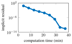
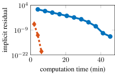
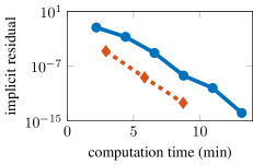
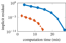

The convergence behavior of NEWTON and RI for the example equations on the data set is illustrated in Figure 1. These and similar plots for the other sparse examples can be found in the accompanying code package [58]. The plots show that for the cases that RI was applicable, it strongly outperformed NEWTON in terms of computation time. This is a result of the choice for the internal CARE solver in RI, which in our experiments was the RADI method [11]. The residuals shown are those that the methods implicitly compute during the iterations to determine convergence. Comparing these plots with Table 8 reveals that the residuals internally computed by RI strongly diverge from the actual normalized residual norm , which is several orders of magnitude larger. On the other hand, for NEWTON the results seem to coincide very well.
5 Conclusions
In this work, we presented a new formulation of the Newton-Kleinman iteration for solving general continuous-time algebraic Riccati equations with large-scale sparse coefficient matrices using low-rank indefinite symmetric factorizations of the solution. For relevant scenarios from the literature, we could show the theoretical convergence of the algorithm. We provided the updated formulas for an exact line search procedure and inexact inner solves, and we outlined how to handle the case of projected algebraic Riccati equations occurring for matrix pencils with infinite eigenvalues. The numerical experiments show that our proposed algorithm provides reliable and accurate solutions to the considered problem and that even in the cases for which we could not provide a convergence theory, the algorithm appears to work perfectly fine.
While we were able to provide convergence results for many of the practically occurring cases, the convergence behavior for the case of indefinite quadratic terms remains unsolved. The numerical results suggest that even in this situation, the proposed Newton-Kleinman method converges to the correct solution, however, the lack of monotonicity in the constructed iterates prevents the use of established strategies for proving convergence. Also, we have observed in our experiments that, while the new Newton-Kleinman iteration outperformed all comparing methods (if there were any at all) in terms of accuracy, it could not compete in the large-scale sparse case with the computational speed of the Riccati iteration that employed the RADI method as inner solver. Therefore, it is in our interest to investigate possible extensions of other, potentially faster performing methods to the case of general algebraic Riccati equations.
References
- [1] G. S. Ammar, P. Benner, and V. Mehrmann. A multishift algorithm for the numerical solution of algebraic Riccati equations. Electron. Trans. Numer. Anal., 1:33–48, 1993. URL: https://etna.math.kent.edu/volumes/1993-2000/vol1/abstract.php?vol=1&pages=33-48.
- [2] B. D. O. Anderson and J. B. Moore. Optimal Control: Linear Quadratic Methods. Prentice-Hall, Englewood Cliffs, NJ, 1990.
- [3] B. D. O. Anderson and B. Vongpanitlerd. Network Analysis and Synthesis: A Modern Systems Approach. Networks Series. Prentice-Hall, Englewood Cliffs, NJ, 1972.
- [4] W. F. Arnold. Numerical solution of algebraic matrix Riccati equations. Tech.-Report ADA139929, Naval Weapons Center, China Lake, CA, 1984. Public reprint of Ph.D. dissertation. URL: https://apps.dtic.mil/sti/citations/ADA139929.
- [5] W. F. Arnold and A. J. Laub. Generalized eigenproblem algorithms and software for algebraic Riccati equations. Proc. IEEE, 72(12):1746–1754, 1984. doi:10.1109/PROC.1984.13083.
- [6] E. Bänsch, P. Benner, J. Saak, and H. K. Weichelt. Riccati-based boundary feedback stabilization of incompressible Navier-Stokes flows. SIAM J. Sci. Comput., 37(2):A832–A858, 2015. doi:10.1137/140980016.
- [7] T. Başar and J. Moon. Riccati equations in Nash and Stackelberg differential and dynamic games. IFAC-Pap., 50(1):9547–9554, 2017. 20th IFAC World Congress. doi:10.1016/j.ifacol.2017.08.1625.
- [8] P. Benner. Contributions to the Numerical Solution of Algebraic Riccati Equations and Related Eigenvalue Problems. PhD thesis, Logos-Verlag, Berlin, 1997.
- [9] P. Benner. Numerical solution of special algebraic Riccati equations via an exact line search method. In 1997 European Control Conference (ECC), pages 3136–3141, 1997. doi:10.23919/ECC.1997.7082591.
- [10] P. Benner and Z. Bujanović. On the solution of large-scale algebraic Riccati equations by using low-dimensional invariant subspaces. Linear Algebra Appl., 488:430–459, 2016. doi:10.1016/j.laa.2015.09.027.
- [11] P. Benner, Z. Bujanović, P. Kürschner, and J. Saak. RADI: a low-rank ADI-type algorithm for large scale algebraic Riccati equations. Numer. Math., 138(2):301–330, 2018. doi:10.1007/s00211-017-0907-5.
- [12] P. Benner, Z. Bujanović, P. Kürschner, and J. Saak. A numerical comparison of different solvers for large-scale, continuous-time algebraic Riccati equations and LQR problems. SIAM J. Sci. Comput., 42(2):A957–A996, 2020. doi:10.1137/18M1220960.
- [13] P. Benner and R. Byers. An exact line search method for solving generalized continuous-time algebraic Riccati equations. IEEE Trans. Autom. Control, 43(1):101–107, 1998. doi:10.1109/9.654908.
- [14] P. Benner, P. Ezzatti, E. S. Quintana-Ortí, and A. Remón. A factored variant of the Newton iteration for the solution of algebraic Riccati equations via the matrix sign function. Numer. Algorithms, 66(2):363–377, 2014. doi:10.1007/s11075-013-9739-2.
- [15] P. Benner, J. Heiland, and S. W. R. Werner. Robust output-feedback stabilization for incompressible flows using low-dimensional -controllers. Comput. Optim. Appl., 82(1):225–249, 2022. doi:10.1007/s10589-022-00359-x.
- [16] P. Benner, J. Heiland, and S. W. R. Werner. A low-rank solution method for Riccati equations with indefinite quadratic terms. Numer. Algorithms, 92(2):1083–1103, 2023. doi:10.1007/s11075-022-01331-w.
- [17] P. Benner, M. Heinkenschloss, J. Saak, and H. K. Weichelt. An inexact low-rank Newton-ADI method for large-scale algebraic Riccati equations. Appl. Numer. Math., 108:125–142, 2016. doi:10.1016/j.apnum.2016.05.006.
- [18] P. Benner, M. Köhler, and J. Saak. Matrix equations, sparse solvers: M-M.E.S.S.-2.0.1—Philosophy, features and application for (parametric) model order reduction. In P. Benner, T. Breiten, H. Faßbender, M. Hinze, T. Stykel, and R. Zimmermann, editors, Model Reduction of Complex Dynamical Systems, volume 171 of International Series of Numerical Mathematics, pages 369–392. Birkhäuser, Cham, 2021. doi:10.1007/978-3-030-72983-7_18.
- [19] P. Benner, P. Kürschner, and J. Saak. Efficient handling of complex shift parameters in the low-rank Cholesky factor ADI method. Numer. Algorithms, 62(2):225–251, 2013. doi:10.1007/s11075-012-9569-7.
- [20] P. Benner, P. Kürschner, and J. Saak. Self-generating and efficient shift parameters in ADI methods for large Lyapunov and Sylvester equations. Electron. Trans. Numer. Anal., 43:142–162, 2014. URL: https://etna.mcs.kent.edu/volumes/2011-2020/vol43/abstract.php?vol=43&pages=142-162.
- [21] P. Benner, J.-R. Li, and T. Penzl. Numerical solution of large-scale Lyapunov equations, Riccati equations, and linear-quadratic optimal control problems. Numer. Lin. Alg. Appl., 15(9):755–777, 2008. doi:10.1002/nla.622.
- [22] P. Benner and J. Saak. Linear-quadratic regulator design for optimal cooling of steel profiles. Technical Report SFB393/05-05, Sonderforschungsbereich 393 Parallele Numerische Simulation für Physik und Kontinuumsmechanik, TU Chemnitz, Chemnitz, Germany, 2005. URL: http://nbn-resolving.de/urn:nbn:de:swb:ch1-200601597.
- [23] P. Benner and J. Saak. Numerical solution of large and sparse continuous time algebraic matrix Riccati and Lyapunov equations: a state of the art survey. GAMM-Mitt., 36(1):32–52, 2013. doi:10.1002/gamm.201310003.
- [24] P. Benner, J. Saak, and S. W. R. Werner. MORLAB – Model Order Reduction LABoratory (version 6.0), September 2023. See also: https://www.mpi-magdeburg.mpg.de/projects/morlab. doi:10.5281/zenodo.7072831.
- [25] P. Benner and T. Stykel. Numerical solution of projected algebraic Riccati equations. SIAM J. Numer. Anal., 52(2):581–600, 2014. doi:10.1137/130923993.
- [26] P. Benner and T. Stykel. Model order reduction for differential-algebraic equations: A survey. In A. Ilchmann and T. Reis, editors, Surveys in Differential-Algebraic Equations IV, Differential-Algebraic Equations Forum, pages 107–160. Springer, Cham, 2017. doi:10.1007/978-3-319-46618-7_3.
- [27] P. Benner and S. W. R. Werner. MORLAB—The Model Order Reduction LABoratory. In P. Benner, T. Breiten, H. Faßbender, M. Hinze, T. Stykel, and R. Zimmermann, editors, Model Reduction of Complex Dynamical Systems, volume 171 of International Series of Numerical Mathematics, pages 393–415. Birkhäuser, Cham, 2021. doi:10.1007/978-3-030-72983-7_19.
- [28] C. Bertram and H. Faßbender. On a family of low-rank algorithms for large-scale algebraic Riccati equations. e-print 2304.01624, arXiv, 2023. Numerical Analysis (math.NA). doi:10.48550/arXiv.2304.01624.
- [29] E. K.-W. Chu, H.-Y. Fan, and W.-W. Lin. A structure-preserving doubling algorithm for continuous-time algebraic Riccati equations. Linear Algebra Appl., 396:55–80, 2005. doi:10.1016/j.laa.2004.10.010.
- [30] M. C. Delfour. Linear quadratic differential games: Saddle point and Riccati differential equation. SIAM J. Control Optim., 46(2):750–774, 2007. doi:10.1137/050639089.
- [31] U. B. Desai and D. Pal. A realization approach to stochastic model reduction and balanced stochastic realizations. In 21st IEEE Conference on Decision and Control, pages 1105–1112, 1982. doi:10.1109/CDC.1982.268322.
- [32] F. Feitzinger, T. Hylla, and E. W. Sachs. Inexact Kleinman-Newton method for Riccati equations. SIAM J. Matrix Anal. Appl., 31(2):272–288, 2009. doi:10.1137/070700978.
- [33] F. Freitas, J. Rommes, and N. Martins. Gramian-based reduction method applied to large sparse power system descriptor models. IEEE Trans. Power Syst., 23(3):1258–1270, 2008. doi:10.1109/TPWRS.2008.926693.
- [34] G. H. Golub and C. F. Van Loan. Matrix Computations. Johns Hopkins Studies in the Mathematical Sciences. Johns Hopkins University Press, Baltimore, fourth edition, 2013.
- [35] M. Heyouni and K. Jbilou. An extended block Arnoldi algorithm for large-scale solutions of the continuous-time algebraic Riccati equation. Electron. Trans. Numer. Anal., 33:53–62, 2009. URL: https://etna.math.kent.edu/volumes/2001-2010/vol33/abstract.php?vol=33&pages=53-62.
- [36] E. A. Jonckheere and L. M. Silverman. A new set of invariants for linear systems–application to reduced order compensator design. IEEE Trans. Autom. Control, 28(10):953–964, 1983. doi:10.1109/TAC.1983.1103159.
- [37] M. Kimura. Doubling algorithm for continuous-time algebraic Riccati equation. Int. J. Syst. Sci., 20(2):191–202, 1989. doi:10.1080/00207728908910119.
- [38] D. L. Kleinman. On an iterative technique for Riccati equation computations. IEEE Trans. Autom. Control, 13(1):114–115, 1968. doi:10.1109/TAC.1968.1098829.
- [39] P. Kürschner. Efficient Low-Rank Solution of Large-Scale Matrix Equations. Dissertation, Otto-von-Guericke-Universität, Magdeburg, Germany, 2016. URL: http://hdl.handle.net/11858/00-001M-0000-0029-CE18-2.
- [40] P. Lancaster and L. Rodman. Algebraic Riccati Equations. Oxford Science Publications. The Clarendon Press, Oxford University Press, New York, 1995.
- [41] N. Lang, H. Mena, and J. Saak. An factorization based ADI algorithm for solving large-scale differential matrix equations. Proc. Appl. Math. Mech., 14(1):827–828, 2014. doi:10.1002/pamm.201410394.
- [42] A. Lanzon, Y. Feng, B. D. .O. Anderson, and M. Rotkowitz. Computing the positive stabilizing solution to algebraic Riccati equations with an indefinite quadratic term via a recursive method. IEEE Trans. Autom. Control, 53(10):2280–2291, 2008. doi:10.1109/TAC.2008.2006108.
- [43] A. J. Laub. A Schur method for solving algebraic Riccati equations. IEEE Trans. Autom. Control, 24(6):913–921, 1979. doi:10.1109/TAC.1979.1102178.
- [44] F. Leibfritz. : COnstrained Matrix-optimization Problem library – a collection of test examples for nonlinear semidefinite programs, control system design and related problems. Tech.-report, University of Trier, 2004. URL: http://www.friedemann-leibfritz.de/COMPlib_Data/COMPlib_Main_Paper.pdf.
- [45] J.-R. Li and J. White. Low rank solution of Lyapunov equations. SIAM J. Matrix Anal. Appl., 24(1):260–280, 2002. doi:10.1137/S0895479801384937.
- [46] Y. Lin and V. Simoncini. A new subspace iteration method for the algebraic Riccati equation. Numer. Linear Algebra Appl., 22(1):26–47, 2015. doi:10.1002/nla.1936.
- [47] A. Locatelli. Optimal Control: An Introduction. Birkhäuser, Basel, 2001.
- [48] Green M. A relative error bound for balanced stochastic truncation. IEEE Trans. Autom. Control, 33(10):961–965, 1988. doi:10.1109/9.7255.
- [49] V. Mehrmann and T. Stykel. Balanced truncation model reduction for large-scale systems in descriptor form. In P. Benner, V. Mehrmann, and D. C. Sorensen, editors, Dimension Reduction of Large-Scale Systems, volume 45 of Lect. Notes Comput. Sci. Eng., pages 83–115. Springer, Berlin, Heidelberg, 2005. doi:10.1007/3-540-27909-1_3.
- [50] D. Mustafa and K. Glover. Controller reduction by -balanced truncation. IEEE Trans. Autom. Control, 36(6):668–682, 1991. doi:10.1109/9.86941.
- [51] Oberwolfach Benchmark Collection. Steel profile. hosted at MORwiki – Model Order Reduction Wiki, 2005. URL: https://morwiki.mpi-magdeburg.mpg.de/morwiki/index.php/Steel_Profile.
- [52] P. C. Opdenacker and E. A. Jonckheere. A contraction mapping preserving balanced reduction scheme and its infinity norm error bounds. IEEE Trans. Circuits Syst., 35(2):184–189, 1988. doi:10.1109/31.1720.
- [53] J. D. Roberts. Linear model reduction and solution of the algebraic Riccati equation by use of the sign function. Internat. J. Control, 32(4):677–687, 1980. Reprint of Technical Report No. TR-13, CUED/B-Control, Cambridge University, Engineering Department, 1971. doi:10.1080/00207178008922881.
- [54] J. Saak and M. Behr. Reimplementation of optimal cooling process for a steel profile of a rail, 2020. URL: https://gitlab.mpi-magdeburg.mpg.de/models/fenicsrail.
- [55] J. Saak and M. Behr. The Oberwolfach steel-profile benchmark revisited, July 2021. doi:10.5281/zenodo.5113560.
- [56] J. Saak, M. Köhler, and P. Benner. M-M.E.S.S. – The Matrix Equations Sparse Solvers library (version 3.0), August 2023. See also: https://www.mpi-magdeburg.mpg.de/projects/mess. doi:10.5281/zenodo.7701424.
- [57] J. Saak and M. Voigt. Model reduction of constrained mechanical systems in M-M.E.S.S. IFAC-Pap., 51(2):661–666, 2018. 9th Vienna International Conference on Mathematical Modelling MATHMOD 2018. doi:10.1016/j.ifacol.2018.03.112.
- [58] J. Saak and S. W. R. Werner. Code, data and results for numerical experiments in “Using factorizations in Newton’s method for solving general large-scale algebraic Riccati equations” (version 1.0), February 2024. doi:10.5281/zenodo.10619037.
- [59] N. Sandell. On Newton’s method for Riccati equation solution. IEEE Trans. Autom. Control, 19(3):254–255, 1974. doi:10.1109/TAC.1974.1100536.
- [60] V. Simoncini. Analysis of the rational Krylov subspace projection method for large-scale algebraic Riccati equations. SIAM J. Matrix Anal. Appl., 37(4):1655–1674, 2016. doi:10.1137/16M1059382.
- [61] E. D. Sontag. Mathematical Control Theory, volume 6 of Texts in Applied Mathematics. Springer, New York, second edition, 1998. doi:10.1007/978-1-4612-0577-7.
- [62] T. Stillfjord. Singular value decay of operator-valued differential Lyapunov and Riccati equations. SIAM J. Control Optim., 56(5):3598–3618, 2018. doi:10.1137/18M1178815.
- [63] T. Stykel. Low-rank iterative methods for projected generalized Lyapunov equations. Electron. Trans. Numer. Anal., 30:187–202, 2008. URL: https://etna.math.kent.edu/volumes/2001-2010/vol30/abstract.php?vol=30&pages=187-202.
- [64] N. Truhar and K. Veselić. An efficient method for estimating the optimal dampers’ viscosity for linear vibrating systems using Lyapunov equation. SIAM J. Matrix Anal. Appl., 31(1):18–39, 2009. doi:10.1137/070683052.
- [65] A. Varga. On computing high accuracy solutions of a class of Riccati equations. Control–Theory and Advanced Technology, 10(4):2005–2016, 1995.
- [66] H. K. Weichelt. Numerical Aspects of Flow Stabilization by Riccati Feedback. Dissertation, Otto-von-Guericke-Universität, Magdeburg, Germany, 2016. doi:10.25673/4493.