RAMP: Boosting Adversarial Robustness Against Multiple $l_{p}$ Perturbations

There is considerable work on improving robustness against adversarial attacks bounded by a single $l_{p}$ norm using adversarial training (AT). However, the multiple-norm robustness (union accuracy) of AT models is still low. We observe that simultaneously obtaining good union and clean accuracy is hard since there are tradeoffs between robustness against multiple $l_{p}$ perturbations, and accuracy/robustness/efficiency. By analyzing the tradeoffs from the lens of distribution shifts, we identify the key tradeoff pair among $l_{p}$ attacks to boost efficiency and design a logit pairing loss to improve the union accuracy. Next, we connect natural training with AT via gradient projection, to find and incorporate useful information from natural training into AT, which moderates the accuracy/robustness tradeoff. Combining our contributions, we propose a framework called RAMP, to boost the robustness against multiple $l_{p}$ perturbations. We show RAMP can be easily adapted for both robust fine-tuning and full AT. For robust fine-tuning, RAMP obtains a union accuracy up to $53.5\%$ on CIFAR-10, and $29.7\%$ on ImageNet. For training from scratch, RAMP achieves SOTA union accuracy of $44.6\%$ and relatively good clean accuracy of $81.2\%$ on ResNet-18 against AutoAttack on CIFAR-10.

Keywords Adversarial Robustness  $\cdot$ Pre-training and Fine-tuning  $\cdot$ Distribution Shifts

1 Introduction

Though Deep Neural Networks (DNNs) demonstrate superior performance in various vision applications, they are vulnerable against adversarial examples (Goodfellow et al., 2014; Kurakin et al., 2018). The most popular defense at present is adversarial training (AT) Tramèr et al. (2017); Madry et al. (2017); adversarial examples are generated and injected into the training process for better robustness. Most AT methods only consider a certain type of perturbation at a time (Wang et al., 2020; Wu et al., 2020; Carmon et al., 2019; Gowal et al., 2020; Raghunathan et al., 2020; Zhang et al., 2021; Debenedetti and Troncoso—EPFL, 2022; Peng et al., 2023; Wang et al., 2023). For example, an $l_{\infty}$ robust model has low robustness against $l_{p}(p\neq\infty)$ attacks (Figure 1(a)). It remains unclear how one can train a model to become more robust against multiple $l_{p}$ perturbations, instead of one (Croce et al., 2020).

There are three main challenges in training models robust against multiple-norm perturbations with good accuracy: (i) tradeoff between robustness against different perturbation models (Tramer and Boneh, 2019), (ii) tradeoff between accuracy and robustness (Zhang et al., 2019; Raghunathan et al., 2020) and (iii) finding the worst-case examples is more expensive than standard AT. Adversarial examples cause a shift from the original distribution, leading to a drop in clean accuracy when performing AT, as mentioned in Xie et al. (2020); Benz et al. (2021). We further observe that the distinct distributions created by $l_{1},l_{2},l_{\infty}$ adversarial examples make the problem even more challenging. Through a finer analysis of the distribution shifts caused by these adversaries, we propose the RAMP framework to efficiently boost the Robustness Against Multiple Perturbations. RAMP can be used for both fine-tuning and training from scratch. It identifies the key tradeoff pair, utilizes a novel logit pairing (Engstrom et al., 2018) loss, and leverages the gradient projection (Jiang et al., 2023) method to improve union accuracy while maintaining good clean accuracy and efficiency.

Identifying the key tradeoff pair. In the multiple-norm setting, one usually triples the computational cost for finding the worst-case examples (Tramer and Boneh, 2019) compared with standard AT, to achieve a good union accuracy. To cut down on the training cost, we analyze $l_{1},l_{2},l_{\infty}$ AT pre-trained models and identify the key $l_{q}-l_{r}$ tradeoff pair for union accuracy, as in Figure 1(a). We first compare the $l_{p}$ robustness of the $l_{p}$-AT model. We select two perturbations where the $l_{p}$-AT model achieves the lowest $l_{p}$ robustness as the key tradeoff pair. For example in Figure 1(a), for the common choices of epsilons on CIFAR-10, we identify $l_{\infty}-l_{1}$ as the key tradeoff pair using this heuristic.

Logit pairing loss. We visualize the changing of $l_{1},l_{2},l_{\infty}$ robustness when fine-tuning a $l_{\infty}$-AT pre-trained model in Figure 1(b). Already after only $1$ epoch of fine-tuning, the DNN loses substantial robustness against $l_{\infty}$ attack: $l_{1}$ fine-tuning (row 2) and E-AT (Croce and Hein, 2022) (row 3) both lose significant $l_{\infty}$ robustness (many points originally colored in cyan turn magenta). Inspired by this observation, we devise a new logit pairing loss for a $l_{q}-l_{r}$ key tradeoff pair, which enforces the logit distributions of $l_{q}$ and $l_{r}$ adversarial examples to be close, specifically on the correctly classified $l_{q}$ subsets. In row 4 of Figure 1(b), we show our method preserves more $l_{\infty}$ robustness than others after $1$ epoch. Further, this technique works on larger models and datasets (Section 5.2).

Gradient projection. To obtain a better accuracy/robustness tradeoff, we explore the connections between natural training (NT) and AT. We find that NT can help with adversarial robustness: there exists useful information in natural distribution, which can be extracted and leveraged to achieve better robustness. To connect NT with AT more effectively, we compare the similarities of model updates of NT and AT layer-wise for each epoch, where we find and incorporate useful NT components into AT via gradient projection, as outlined in Algorithm 2. In Figure 2 and Section 5.2, we empirically show this technique strikes a better balance between accuracy and robustness, for both single and multiple $l_{p}$ perturbations. We provide theoretical insights into why GP works in Theorem 1.

Main contributions:

• We analyze tradeoffs between robustness against different $l_{p}$ perturbations and accuracy/robustness from the lens of distribution shifts, along with attaining good efficiency at the same time.

• We identify the key $l_{q}-l_{r}$ tradeoff pair to improve the efficiency, design a new logit pairing loss to mitigate the $l_{q}-l_{r}$ tradeoff for better union accuracy, and use gradient projection to balance the accuracy/robustness tradeoff for multiple $l_{p}$ perturbations.

• We show our RAMP framework achieves SOTA union accuracy for both robust fine-tuning and training from scratch. RAMP fine-tunes DNNs achieving union accuracy up to $53.5\%$ on CIFAR-10, and $29.7\%$ on ImageNet. For training from scratch, RAMP achieves SOTA union accuracy of $44.6\%$ and relatively good clean accuracy of $81.2\%$ on ResNet-18 against AutoAttack on CIFAR-10.

Our code is available at  https://github.com/uiuc-focal-lab/RAMP.

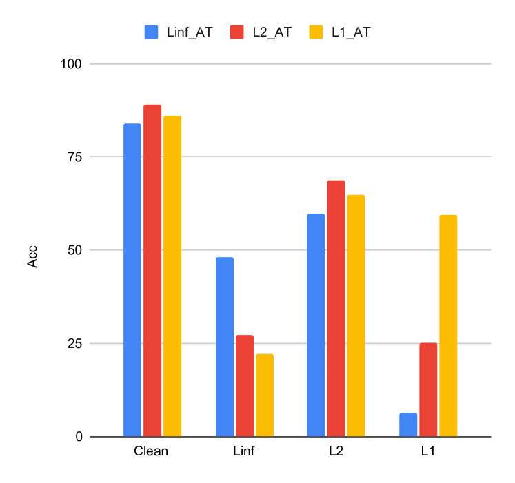
(a) Multiple-norm tradeoff with $l_{1},l_{2},l_{\infty}$ AT pre-trained models (colored in blue, red, and orange respectively), with respect to their clean accuracy (y-axis), and robust accuracy (y-axis) against $l_{\infty},l_{2},l_{1}$ attacks on the x-axis. Here we use $\epsilon_{1}=12,\epsilon_{2}=0.5,\epsilon_{\infty}=\frac{8}{255}$.

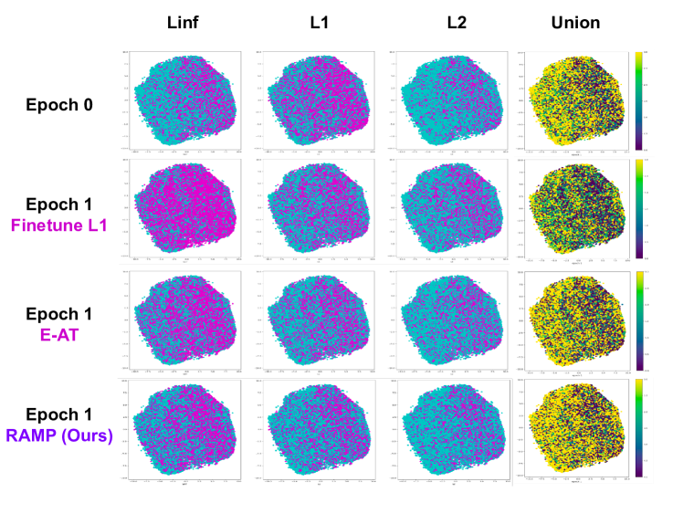
(b) Multiple-norm tradeoff with robust fine-tuning: For a single $l_{p}$ attack, correct predictions are colored with cyan and incorrect with magenta. For the union accuracy, the yellow color refers to the robustness against three perturbations. The rows show the multiple-norm robustness of (1) $l_{\infty}$-AT model (epoch 0), (2) after $1$ epoch of fine-tuning on $l_{1}$ examples, (3) after $1$ epoch of E-AT fine-tuning, (4) after $1$ epoch of RAMP fine-tuning.

Figure 1: A finer analysis on $l_{1},l_{2},l_{\infty}$ tradeoff. (a) We identify the $l_{1}-l_{\infty}$ as the key tradeoff pair. (b) We observe that fine-tuning on $l_{\infty}$-AT model using $l_{1}$ examples drastically reduces $l_{\infty}$ robustness. RAMP can preserve more $l_{\infty}$ robustness after robust fine-tuning.

2 Related Work

Adversarial training (AT). AT finds adversarial examples via gradient descent and includes them in training to improve adversarial robustness (Tramèr et al., 2017; Madry et al., 2017). There are a large number of works on boosting robustness, based on exploring robustness/accuracy trade-off (Zhang et al., 2019; Wang et al., 2020), instance reweighting (Zhang et al., 2021), loss landscapes (Wu et al., 2020), wider/larger architectures (Gowal et al., 2020; Debenedetti and Troncoso—EPFL, 2022), data augmentation (Carmon et al., 2019; Raghunathan et al., 2020), and using synthetic data (Peng et al., 2023; Wang et al., 2023). However, most DNNs they obtain are robust against a single perturbation type and are vulnerable to other types.

Robustness against multiple perturbations. Tramer and Boneh (2019); Kang et al. (2019) discovered the tradeoff between different perturbation types: robustness against $l_{p}$ attack does not transfer well to another $l_{q}(q\neq p)$ attack. Since there are prior works (Tramer and Boneh, 2019; Maini et al., 2020; Madaan et al., 2021; Croce and Hein, 2022) modifying the AT training scheme to improve robustness against multiple $l_{p}$ attacks, via average-case (Tramer and Boneh, 2019), worst-case (Tramer and Boneh, 2019; Maini et al., 2020), and random-sampled (Madaan et al., 2021; Croce and Hein, 2022) defenses. Furthermore, Croce and Hein (2022) devise Extreme norm Adversarial Training (E-AT) and fine-tune a $l_{p}$ robust model on another $l_{q}$ perturbation to quickly make a DNN robust against multiple $l_{p}$ attacks. However, E-AT (Croce and Hein, 2022) does not adapt to varying epsilon values. Also, we show that the tradeoff between robustness against different $l_{p}$ attacks achieved by prior works is suboptimal and can be improved by our proposed framework.

Logit pairing in adversarial training. Adversarial logit pairing methods (Kannan et al., 2018; Engstrom et al., 2018) were proposed to devise a stronger form of adversarial training. Prior works apply this technique to both clean and adversarial counterparts. In our work, we apply logit pairing to train a DNN originally robust against $l_{p}$ attack to become robust against another $l_{q}(q\neq p)$ attack on the correctly predicted $l_{p}$ subsets, which helps gain better union accuracy.

Adversarial versus distributional robustness.  Sinha et al. (2018) theoretically studies the AT problem from the perspective of distributional robust optimization. There also exists a line of works investigating the connection between natural distribution shifts and adversarial distribution shifts (Moayeri et al., 2022; Alhamoud et al., 2023). They measure and explore the transferability and generalizability of adversarial robustness among different datasets with natural distribution shifts. However, to the best of our knowledge, there is little work exploring distribution shifts created by adversarial examples and how this connects with the tradeoff between robustness and accuracy Zhang et al. (2019); Yang et al. (2020); Rade and Moosavi-Dezfooli (2021) - training on adversarial examples degrades the original clean accuracy. In our work, inspired by the recent work on domain adaptation to better combine source and target gradients (Jiang, 2023; Jiang et al., 2023), we show how to leverage the model updates of natural training (source domain) to help adversarial robustness (target domain).

3 AT against Multiple Perturbations

We consider a standard classification task with samples $\{(x_{i},y_{i})\}_{i=0}^{N}$ from a data distribution $\mathcal{D}$; we have input images $x\in\mathbb{R}^{d}$ and corresponding labels $y\in\mathbb{R}^{k}$. Standard training aims to obtain a classifier $f$ parameterized by $\theta$ to minimize a loss function $\mathcal{L}:\mathbb{R}^{k}\times\mathbb{R}^{k}\rightarrow\mathbb{R}$ on $\mathcal{D}$. Adversarial training (AT) (Madry et al., 2017; Tramèr et al., 2017) aims to find a DNN robust against adversarial examples. It is framed as a min-max problem where a DNN is optimized using the worst-case examples within an adversarial region around each $x_{i}$. Different types of adversarial regions $B_{p}(x,\epsilon_{p})=\{x^{\prime}\in\mathbb{R}^{d}:\|x^{\prime}-x\|_{p}\leq\epsilon_{p}\}$ can be defined around a given image $x$ using various $l_{p}$-based perturbations. Formally, we can write the optimization problem of AT against a certain $l_{p}$ attack as follows:

$$\min_{\theta}\mathbb{E}_{(x,y)\sim\mathcal{D}}\left[\max_{x^{\prime}\in B_{p}(x,\epsilon_{p})}\mathcal{L}(f(x^{\prime}),y)\right]$$

The above optimization is only for specific $p$ values and is usually vulnerable to other perturbation types. To this end, prior works have proposed several approaches to train the network robust against multiple perturbations ($l_{1},l_{2},l_{\infty}$) at the same time. Thus, we focus on the union threat model $\Delta=B_{1}(x,\epsilon_{1})\cup B_{2}(x,\epsilon_{2})\cup B_{\infty}(x,\epsilon_{\infty})$ which requires the DNN to be robust within the $l_{1},l_{2},l_{\infty}$ adversarial regions simultaneously (Croce and Hein, 2022). Union accuracy is then defined as the robustness against $\Delta_{i}$ for each $x_{i}$ sampled from $\mathcal{D}$. In this paper, similar to the prior works, we use union accuracy as the main metric to evaluate the multiple-norm robustness. There are three main categories of defenses: 1. Worst-case, 2. Average-case, and 3. Random-sampled defenses.

Worst-case defense. The DNN is optimized using the worst-case example from the $l_{1},l_{2},l_{\infty}$ adversarial regions:

$$\min_{\theta}\mathbb{E}_{(x,y)\sim\mathcal{D}}\left[\max_{p\in\{1,2,\infty\}}\max_{x^{\prime}\in B_{p}(x,\epsilon_{p})}\mathcal{L}(f(x^{\prime}),y)\right]$$

MAX (Tramer and Boneh, 2019) and MSD (Maini et al., 2020) fall into this category, where MSD is more fine-grained as it finds the worst-case examples with the highest loss during each step of inner maximization. Finding worst-case examples yields a good union accuracy but usually results in a loss of clean accuracy as the generated examples can be different from the original distribution.

Average-case defense. The DNN is optimized using the average of the $l_{1},l_{2},l_{\infty}$ worst-case examples:

$$\min_{\theta}\mathbb{E}_{(x,y)\sim\mathcal{D}}\left[\mathbb{E}_{p\in\{1,2,\infty\}}\max_{x^{\prime}\in B_{p}(x,\epsilon_{p})}\mathcal{L}(f(x^{\prime}),y)\right]$$

AVG (Tramer and Boneh, 2019) is of this type. It is not suited for union accuracy as it less penalizes worst-case behavior within the $l_{1},l_{2},l_{\infty}$ regions. However, this defense usually has relatively good clean accuracy.

Random-sampled defense. The defenses mentioned above lead to a high training cost as they compute multiple attacks for each sample. SAT (Madaan et al., 2021) and E-AT (Croce and Hein, 2022) randomly sample one attack out of three or two types at a time, contributing to a similar computational cost as standard AT on a single perturbation. They achieve a slightly better union accuracy compared with AVG and relatively good clean accuracy. However, they are not better than worst-case defenses for multiple-norm robustness, since they still lack consideration for the strongest attack within the union region.

4 RAMP

There are three main tradeoffs in achieving better union accuracy while maintaining good accuracy and efficiency: 1. Among perturbations: there is a tradeoff between three attacks, e.g., a $l_{\infty}$ pre-trained AT DNN is not robust against $l_{1},l_{2}$ perturbations and vice versa (Figure 1(a)), which makes the union accuracy harder to attain. 2. Accuracy and robustness: all defenses lead to degraded clean accuracy. 3. Performance and efficiency: finding the worst-case examples triples the computational cost compared with standard AT. To address these tradeoffs, we study the problem from the lens of distribution shifts.

Interpreting tradeoffs from the lens of distribution shifts. The adversarial examples with respect to a data distribution $\mathcal{D}$, adversarial region $B_{p}(x,\epsilon_{p})$, and DNN $f_{\theta}$ generate a new adversarial distribution $\mathcal{D}^{\prime}$ with samples $\{(x^{\prime}_{i},y_{i})\}_{i=0}^{N}$, that are correlated but different from the original $\mathcal{D}$. Because of the inherent shifts between $\mathcal{D}$ and $\mathcal{D}^{\prime}$, it decreases performance on $\mathcal{D}$ when we move away from it and towards $\mathcal{D^{\prime}}$. Also, the distinct distributions created by multiple perturbations, $\mathcal{D^{\prime}}_{l_{1}}$, $\mathcal{D^{\prime}}_{l_{2}}$, $\mathcal{D^{\prime}}_{l_{\infty}}$, contribute to the tradeoff among $l_{1},l_{2},l_{\infty}$ attacks. To address the tradeoff among perturbations while maintaining good efficiency, we focus on the distributional interconnections between $\mathcal{D}$ and its adversarial counterparts $\mathcal{D^{\prime}}_{l_{1}}$, $\mathcal{D^{\prime}}_{l_{2}}$, $\mathcal{D^{\prime}}_{l_{\infty}}$.

From the insights we get from the above analysis, we propose our framework RAMP, which includes (i) identifying the key tradeoff pair to improve efficiency, (ii) logit pairing to improve tradeoffs among multiple perturbations, and (iii) identifying and combining the useful DNN components by comparing the model updates from natural training and AT, to obtain a better robustness/accuracy tradeoff. RAMP can achieve a better union accuracy for both robust fine-tuning and AT from random initialization (Section 5.2) with relatively good efficiency. In Section 4.1 and Section 4.2, we study the distribution shifts among the adversarial regions from multiple perturbations. In Section 4.3, we study the distribution shifts between $\mathcal{D}$ and $\mathcal{D}^{\prime}$ to mitigate the accuracy/robustness tradeoff.

4.1 Identify the Key Tradeoff Pair for Better Efficiency

As an example, we study the common case of the multiple-norm tradeoff when $\epsilon_{1}=12,\epsilon_{2}=0.5,\epsilon_{\infty}=\frac{8}{255}$ on CIFAR-10 (Tramer and Boneh, 2019). In Figure 1(a), we compare the pre-trained versions of AT models on $l_{1},l_{2},l_{\infty}$ attacks (colored in blue, red, and orange respectively) with respect to their clean accuracy (y-axis) on the original $\mathcal{D}$, and robust accuracy (y-axis) against $l_{\infty},l_{2},l_{1}$ attacks on the x-axis. We see the robust accuracy against $l_{2}$ attack is the highest compared with $l_{1}$ and $l_{\infty}$ on the three pre-trained models.  Croce and Hein (2022) shows this phenomenon does not depend on the DNN architecture. This means $\mathcal{D}^{\prime}_{l_{2}}$ has a smaller distribution shift from $\mathcal{D}^{\prime}_{l_{1}}$ and $\mathcal{D}^{\prime}_{l_{\infty}}$. Thus the robustness against $l_{2}$ attack is not the bottleneck for achieving better union accuracy and this type of robustness usually can be gained when we train on other $l_{1},l_{\infty}$ adversarial examples. Also, we observe that $l_{\infty}$ pre-trained AT model has a low $l_{1}$ robust accuracy and vice versa. The $l_{1}$ and $l_{\infty}$ robust accuracy gaps are $37.4\%$ for $l_{1}$-AT model and $41.8\%$ for $l_{\infty}$-AT model, which means $\mathcal{D}^{\prime}_{l_{1}}$ and $\mathcal{D}^{\prime}_{l_{\infty}}$ are distinctly different. Intuitively speaking, one may lose significant robustness on $l_{\infty}$ when training with $l_{1}$ examples, because of the large distribution shifts between the two. Therefore, in this common case, we identify $l_{\infty}-l_{1}$ as the key tradeoff pair for the multiple-norm robustness.

A more general heuristic. The key tradeoff pair will change when we choose varying epsilon values for multiple perturbations, as shown in Figure 2. To provide a more general heuristic to identify the key tradeoff pair, we first compare the $l_{p}$ robustness of the $l_{p}$-AT model for $l_{1},l_{2},l_{\infty}$ attacks. In other words, we compare the robustness of pre-trained AT models against its own attack. We select two perturbations where the $l_{p}$-AT model achieves the lowest $l_{p}$ robustness as the key tradeoff pair. We identify the trade-off pair with the perturbations having lower robust accuracy (box colored in purple and green) causing larger distribution shifts.

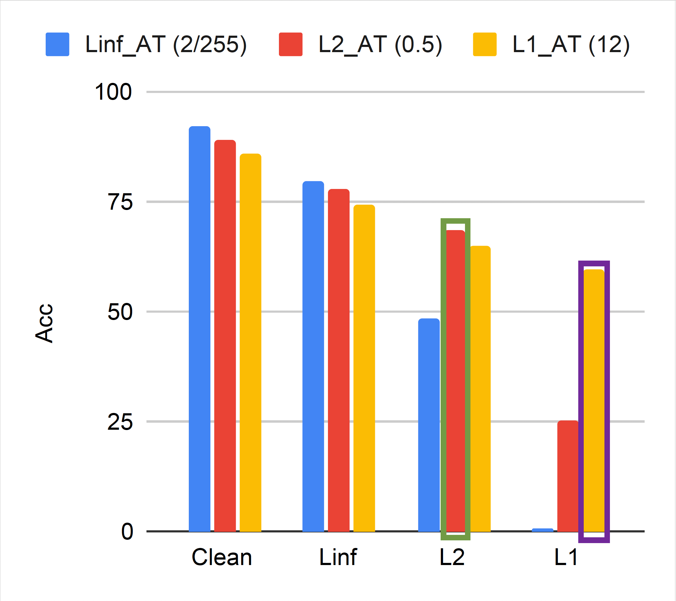
(a) $l_{1}$ - $l_{2}$ trade-off: $l_{1}$-AT model has the lowest $l_{1}$ robustness (box colored in purple), which is included in the tradeoff pair and serves as the starting point of robust fine-tuning. $l_{2}$-AT model has the second lowest $l_{2}$ robustness (box colored in green) and is the other perturbation in the tradeoff pair.

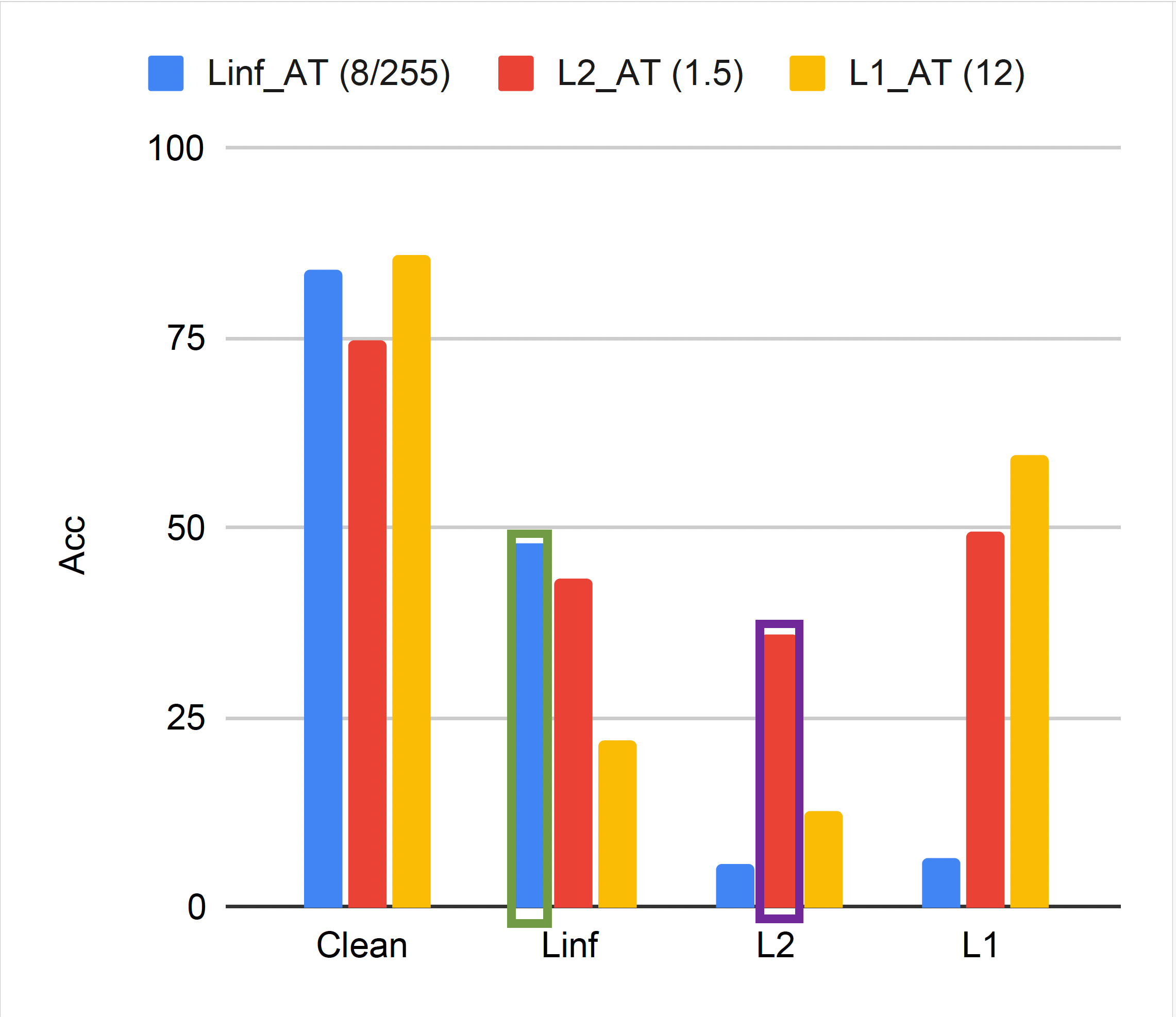
(b) $l_{2}$ - $l_{\infty}$ trade-off: $l_{2}$-AT model has the lowest $l_{2}$ robustness (box colored in purple), which is included in the tradeoff pair and serves as the starting point of robust fine-tuning. $l_{\infty}$-AT model has the second lowest $l_{\infty}$ robustness (box colored in green) and is the other perturbation in the tradeoff pair.

Figure 2: Two special cases when the key trade-off pair changes compared with standard values used in literature.

4.2 Logit Pairing for Multiple Perturbations

Figure 1(b): Finetuning a $l_{q}$-AT model on $l_{r}$ examples reduces $l_{q}$ robustness. To get a finer analysis of the $l_{\infty}-l_{1}$ tradeoff mentioned above, we visualize the changing of $l_{1},l_{2},l_{\infty}$ robustness when we fine-tune a $l_{\infty}$ pre-trained model with $l_{1}$ examples for $3$ epochs, as shown in the second row of Figure 1(b). Here we project each image into a 2D plane using the t-SNE plot and color them with correct or incorrect predictions. For an individual attack, correct ones are colored in cyan, incorrect ones are colored in magenta; for union accuracy, correct ones are colored in yellow. Surprisingly, we find that only after the $1$ epoch of robust fine-tuning, the new DNN loses the $l_{\infty}$ robustness fairly quickly with more points colored in magenta against $l_{\infty}$ attack. The above observations indicate the necessity of preserving more $l_{q}$ robustness as we adversarially fine-tune with $l_{r}$ adversarial examples on a pre-trained AT model, with $l_{q}-l_{r}$ as the key tradeoff pair. This insight inspires us to design our loss design with logit pairing. We want to enforce the union predictions between $l_{q}$ and $l_{r}(q\neq r)$ attacks: bringing the predictions of $l_{q}$ and $l_{r}(q\neq r)$ close to each other, specifically on the correctly predicted $l_{q}$ subsets.

Based on our observations from the analysis, we design a new logit pairing loss to enforce a DNN robust against one $l_{q}$ attack to be robust against another $l_{r}(q\neq r)$ attack.

4.2.1 Enforcing the Union Prediction via Logit Pairing

The $l_{q}-l_{r}(q\neq r)$ tradeoff leads us to the following principle to improve union accuracy: for a given set of images, when we have a DNN robust against some $l_{q}$ examples, we want it to be robust against $l_{r}$ examples as well. This serves as the main insight for our loss design: we want to enforce the logits predicted by $l_{q}$ and $l_{r}$ adversarial examples to be close, specifically on the correctly predicted $l_{q}$ subsets. To accomplish this, we design a KL-divergence (KL) loss between the predictions from $l_{q}$ and $l_{r}$ perturbations. For each batch of data $(x,y)\sim\mathcal{D}$, we generate $l_{q}$ and $l_{r}$ adversarial examples $x^{\prime}_{q},x^{\prime}_{r}$ and their predictions $p_{q},p_{r}$ using APGD Croce and Hein (2020). Then, we select indices $\gamma$ for which $p_{q}$ correctly predicts the ground truth $y$. We denote the size of the indices as $n_{c}$, and the batch size as $N$. We compute a KL-divergence loss over this set of samples using $KL(p_{q}[\gamma]\|p_{r}[\gamma])$ (Eq. 1). For the subset indexed by $\gamma$, we want to push its $l_{r}$ logit distribution towards its $l_{q}$ logit distribution, such that we prevent losing more $l_{q}$ robustness when training with $l_{r}$ adversarial examples.

$$\mathcal{L}_{KL}=\frac{1}{n_{c}}\cdot\sum^{n_{c}}_{i=0}p_{q}[\gamma[i]]\cdot\log\left(\frac{p_{q}[\gamma[i]]}{p_{r}[\gamma[i]]}\right)$$ (1)

To further boost the union accuracy, apart from the KL loss, we add another loss term using a MAX-style approach in Eq. 2: we find the worst-case example between $l_{q}$ and $l_{r}$ adversarial regions by selecting the example with the higher loss. $\mathcal{L}_{max}$ is a cross-entropy loss over the approximated worst-case adversarial examples. Here, we use $\mathcal{L}_{ce}$ to represent the cross-entropy loss.

$$\mathcal{L}_{max}=\frac{1}{N}\sum^{N}_{i=0}\left[\max_{p\in\{q,r\}}\max_{x_{i}^{\prime}\in B_{p}(x,\epsilon_{p})}\mathcal{L}_{ce}(f(x_{i}^{\prime}),y_{i})\right]$$ (2)

Our final loss $\mathcal{L}$ combines $\mathcal{L}_{KL}$ and $\mathcal{L}_{max}$, via a hyper-parameter $\lambda$, as shown in Eq. 3.

$$\mathcal{L}=\mathcal{L}_{max}+\lambda\cdot\mathcal{L}_{KL}$$ (3)

Algorithm 1 Robust Fine-tuning with Logit Pairing

1:  Input: model $f$, input samples $(x,y)$ from distribution $\mathcal{D}$, fine-tuning rounds $R$, hyper-parameter $\lambda$, adversarial regions $B_{q},B_{r}$ with size $\epsilon_{q}$ and $\epsilon_{r}$, APGD attack.

2:  for $r=1,2,...,R$ do

3:     for $(x,y)\sim\text{ training set }\mathcal{D}$ do

4:        $x^{\prime}_{q},p_{q}\leftarrow\textbf{APGD}(B_{q}(x,\epsilon_{q}),y)$

5:        $x^{\prime}_{r},p_{r}\leftarrow\textbf{APGD}(B_{r}(x,\epsilon_{r}),y)$

6:        $\gamma\leftarrow where(p_{q}.max=y)$

7:        $n_{c}\leftarrow\gamma.size()$

8:        calculate $\mathcal{L}$ using Eq. 3 and update $f$

9:     end for

10:  end for

11:  Output: model $f$.

Algorithm 1 shows the pseudocode of robust fine-tuning with RAMP that leverages logit pairing.

4.3 Connecting Natural Training with AT

To improve the robustness and accuracy tradeoff against multiple perturbations, we explore the connections between AT and natural training (NT), where we discover there exists some useful information in NT that helps improve robustness. To extract the useful components from NT and incorporate them into the AT procedure, we leverage gradient projection (Jiang et al., 2023) to compare and combine the natural and adversarial model updates, where we manage to obtain a better robustness and accuracy tradeoff.

4.3.1 NT can help adversarial robustness

Let us consider two models $f_{1}$ and $f_{2}$, where $f_{1}$ is randomly initialized and $f_{2}$ is trained with natural training on $\mathcal{D}$ for $k$ epochs. $f_{2}$ has a better decision boundary than $f_{1}$, leading to higher clean accuracy. When we perform AT on $f_{1}$ and $f_{2}$ afterward, intuitively speaking, $f_{2}$ will become more robust than $f_{1}$ - it misclassifies less adversarial examples because of the better decision boundary. We empirically show this effect in Figure 3. For AT (blue), we perform the standard AT against $l_{\infty}$ attack (Madry et al., 2017) and for AT-pre (red), we perform $50$ epochs of pre-training before the standard AT procedure. From the figure, we see AT-pre has better clean and robust accuracy than AT on CIFAR-10 against $l_{\infty}$ PGD-20 attack with $\epsilon_{\infty}=0.031$. From the distributional perspective, though $\mathcal{D}$ and $\mathcal{D^{\prime}}$ are different, based on our observation in Figure 3, there exists useful information in the original distribution $\mathcal{D}$, which can be potentially leveraged to improve the performance on $\mathcal{D^{\prime}}$.

4.3.2 AT with Gradient Projection

To connect NT with AT more effectively, we take a closer look at the training procedure on $\mathcal{D}$ and $\mathcal{D^{\prime}}$. We consider the model updates over all samples from $\mathcal{D}$ and $\mathcal{D^{\prime}}$, where we define the initial model $f^{(r)}$ at epoch $r$, and the models $f_{n}^{(r)}$, and $f_{a}^{(r)}$ after $1$ epoch of natural training and adversarial training from the same starting point $f^{(r)}$, respectively. Here, we compare the natural updates $g_{n}=f_{n}^{(r)}-f^{(r)}$ and adversarial updates $g_{a}=f_{a}^{(r)}-f^{(r)}$: they are different because of the distribution shift, and there exists an angle between them. We want to find the useful components from $g_{n}$ and combine them into $g_{a}$, so we can gain more robustness in $\mathcal{D}^{\prime}$ as well as preserve accuracy in $\mathcal{D}$.

Inspired by Jiang et al. (2023), we compare the model updates layer-wise by computing the cosine similarity between $g_{n}$ and $g_{a}$. For a certain layer $l$ of $g_{n}^{l}$ and $g_{a}^{l}$, we preserve a certain portion of $g_{n}^{l}$ using their cosine similarity score (Eq. 4). If the score is negative, it means $g_{n}^{l}$ is not helpful for robustness in $\mathcal{D^{\prime}}$, thus we filter out the useless components that have a similarity score $\leq 0$. If the score is high, we want to preserve a larger portion of it. We define GP (Gradient Projection) operation in Eq. 5 by projecting $g_{a}^{l}$ towards $g_{n}^{l}$.

$$\cos(g_{n}^{l},g_{a}^{l})={g_{n}^{l}\cdot g_{a}^{l}\over\|g_{n}^{l}\|\|g_{a}^{l}\|}$$ (4)

$$\mathbf{GP}(g_{n}^{l},g_{a}^{l})=\begin{cases}\cos(g_{n}^{l},g_{a}^{l})\cdot g_{n}^{l},&\cos(g_{n}^{l},g_{a}^{l})>0\\ 0,&\cos(g_{n}^{l},g_{a}^{l})\leq 0\end{cases}$$ (5)

To sum up, the total projected (useful) model updates $g_{GP}$ coming from $g_{n}$ could be computed as Eq. 6. We use $\mathcal{M}$ to denote all layers of the current model update. Note that $\bigcup_{l\in\mathcal{M}}$ concatenates the useful natural model update components of all layers.

$$g_{GP}=\bigcup_{l\in\mathcal{M}}\left(\mathbf{GP}(g_{n}^{l},g_{a}^{l})\right)$$ (6)

$$f^{(r+1)}=f^{(r)}+(1-\beta)\cdot g_{GP}+\beta\cdot g_{a}$$ (7)

A hyper-parameter $\beta$ is used to balance the contributions of $g_{GP}$ and $g_{a}$, as shown in Eq. 7. By finding a proper $\beta$ (usually 0.5 as in Figure 4(c)), we can obtain better robustness on $\mathcal{D^{\prime}}$, as shown in Figure 3 and Table 1. In Figure 3, with $\beta=0.5$, AT-GP (orange) refers to AT with GP; for AT-GP-pre (green), we perform $50$ epochs of NT before doing AT-GP. We see AT-GP obtains a better accuracy/robustness tradeoff than AT. We observe a similar trend for AT-GP-pre vs. AT-pre. Further, in Table 1, RN-18 $l_{\infty}$-GP achieves good clean accuracy and better robustness than RN-18 $l_{\infty}$ against $l_{\infty}$ AutoAttack with $\epsilon=\frac{8}{255}$. Also, we achieve a good clean accuracy by preserving model updates in $\mathcal{D}$.

Theoretical insights of Gradient Projection (GP). We denote ${\mathcal{D}}_{a}$ as the distribution created by adversarial examples generated on a perfect classifier, trained on an infinite number of examples. $\widehat{\mathcal{D}}_{a}$ is the distribution created by adversarial examples generated by the adversarially trained (AT) classifier using limited clean images. $\widehat{\mathcal{D}}_{n}$ is the distribution of original clean images. We define the model updates per epoch on these distributions as $g_{a},\widehat{g_{a}},\widehat{g}_{n}$, respectively; $g_{GP}$ is the model update using GP for one epoch. Delta errors $\Delta^{2}_{{AT}}$ and $\Delta^{2}_{{GP}}$ measure the closesness of $g_{GP},\widehat{g_{a}}$ from $g_{a}$ in $\widehat{\mathcal{D}}_{a}$ ($\Delta^{2}_{{Aggr}}:=\mathbb{E}_{\widehat{\mathcal{D}}_{a}}\|g_{a}-g_{{Aggr}}\|^{2}_{\pi}$, where $g_{{Aggr}}=g_{GP}$ or $g_{{Aggr}}=\widehat{g_{a}}$) each iteration. Further, we define $\bar{\tau}^{2}=\mathbb{E}_{\pi}[\tau^{2}]\in[0,1]$, where $\tau$ is the $\sin(\cdot)$ value of the angle between $\widehat{g}_{n}$ and $g_{a}-\widehat{g}_{n}$. Theorem 1 shows $\Delta^{2}_{{GP}}$ is usually smaller than $\Delta^{2}_{{AT}}$ for a large model dimension, since $(1-\beta^{2}\bar{\tau}^{2})\geq(1-\beta^{2})$ and we have an additional positive term $2\beta\|g_{a}-\widehat{g}_{n}\|^{2}_{\pi}$. Thus, GP can usually achieve better robust accuracy than AT by achieving a smaller error rate each epoch; GP also obtains good clean accuracy by combining parts of the model updates from the clean distribution ${\mathcal{D}}_{n}$. The full proof are in Appendix A.

Theorem 1 (Error Analysis of GP).

When the model dimension is large, we have

$$\Delta^{2}_{{AT}}-\Delta^{2}_{{GP}}\approx\left((1-\beta^{2}\bar{\tau}^{2})\mathbb{E}_{\widehat{\mathcal{D}}_{a}}\|g_{a}-\widehat{g}_{a}\|^{2}_{\pi}-(1-\beta^{2})\|g_{a}-\widehat{g}_{n}\|^{2}_{\pi}\right)+2\beta\|g_{a}-\widehat{g}_{n}\|^{2}_{\pi}$$

where $\|\cdot\|_{\pi}$ is the $\pi$-norm over the model parameter space.

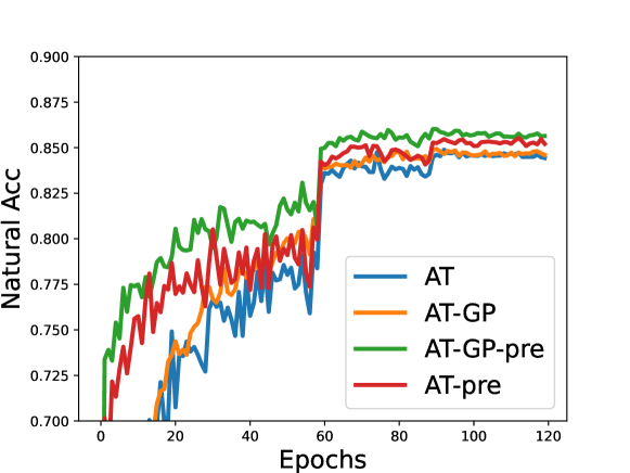
(a) Clean Accuracy

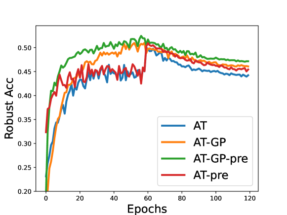
(b) Robust Accuracy: PGD-20

Figure 3: $l_{\infty}$ AT-GP with PGD (Madry et al., 2017) of $\epsilon=0.031$ on CIFAR-10 improves both accuracy and robustness. With pre-training on $\mathcal{D}$ for $50$ epochs, we can further boost the performance.

	Clean	$l_{\infty}$
RN-18 $l_{\infty}$	$84.2$	$47.4$
RN-18 $l_{\infty}$-GP	$84.5$	$\bf 48.3$
RN-18 $l_{\infty}$-GP-pre	$\bf 84.9$	$\bf 48.3$

Table 1: $l_{\infty}$ AT-GP with APGD (Croce and Hein, 2020) improves robustness against $l_{\infty}$ AutoAttack with $\epsilon=\frac{8}{255}$. RN-18 $l_{\infty}$-GP uses AT-GP; RN-18 $l_{\infty}$-GP-pre pre-trains $40$ epochs on $\mathcal{D}$ before AT-GP is applied.

We outline the AT-GP method in Algorithm 2 and it can be extended to the multiple-norm scenario, which we discuss in Section 4.4. The overhead of this algorithm comes from natural training and GP operation. Their costs are small, and we discuss this more in Section 5.4.

Algorithm 2 Adversarial Training with Gradient Projection

1:  Input: model $f$, input images with distribution $\mathcal{D}$, training rounds $R$, adversarial region $B_{p}$ and its size $\epsilon_{p}$, $\beta$, natural training NT and adversarial training AT.

2:  for $r=1,2,...,R$ do

3:     $f_{n}\leftarrow\textbf{NT}(f^{(r)},\mathcal{D})$

4:     $f_{a}\leftarrow\textbf{AT}(f^{(r)},B_{p},\epsilon_{p},\mathcal{D})$

5:     compute $g_{n}\leftarrow f_{n}-f^{(r)}$, $g_{a}\leftarrow f_{a}-f^{(r)}$

6:     compute $g_{GP}$ using Eq. 6

7:     update $f^{(r+1)}$ using Eq. 7 with $\beta$ and $g_{a}$

8:  end for

9:  Output: model $f$.

4.4 RAMP Algorithm

Combining logit pairing and gradient projection methods, we provide a framework for boosting the Robustness Against Multiple Perturbations (RAMP), which is similar to Algorithm 2. The only difference is that we replace the standard AT procedure of getting $f_{adv}$ (line 4 of Algorithm 2) as Algorithm 1. We show that DNNs trained or fine-tuned using RAMP achieve state-of-the-art union accuracy (Section 5.2).

5 Experiment

Methods	Clean	$l_{\infty}$	$l_{2}$	$l_{1}$	Union
RN-18- $l_{\infty}$-AT	$83.7$	$48.1$	$59.8$	$7.7$	$38.5$
+ SAT	$83.5\pm 0.2$	$43.5\pm 0.2$	$68.0\pm 0.4$	$47.4\pm 0.5$	$41.0\pm 0.3$
+ AVG	$84.2\pm 0.4$	$43.3\pm 0.4$	$68.4\pm 0.6$	$46.9\pm 0.6$	$40.6\pm 0.4$
+ MAX	$82.2\pm 0.3$	$45.2\pm 0.4$	$67.0\pm 0.7$	$46.1\pm 0.4$	$42.2\pm 0.6$
+ MSD	$82.2\pm 0.4$	$44.9\pm 0.3$	$67.1\pm 0.6$	$47.2\pm 0.6$	$42.6\pm 0.2$
+ E-AT	$82.7\pm 0.4$	$44.3\pm 0.6$	$68.1\pm 0.5$	$48.7\pm 0.5$	$42.2\pm 0.8$
+ RAMP	$81.1\pm 0.2$	$45.4\pm 0.3$	$66.1\pm 0.2$	$47.2\pm 0.1$	$\mathbf{43.1\pm 0.2}$

Table 2: RN-18 $l_{\infty}$-AT model fine-tuned with different methods for 3 epochs (repeated for 5 seeds). RAMP has the highest union accuracy. Baseline results are from Croce and Hein (2022).

	Models	Methods	Clean	$l_{\infty}$	$l_{2}$	$l_{1}$	Union
	WRN-70-16-$l_{\infty}$(*) (Gowal et al., 2020)	E-AT	91.6	54.3	78.2	58.3	51.2
		RAMP	91.2	54.9	75.3	58.8	53.5
	WRN-34-20-$l_{\infty}$ (Gowal et al., 2020)	E-AT	88.3	49.3	71.8	51.2	46.2
		RAMP	87.9	49.3	70.5	51.2	47.5
	WRN-28-10-$l_{\infty}$(*) (Carmon et al., 2019)	E-AT	90.3	52.6	74.7	54.0	48.7
CIFAR-10		RAMP	90.3	51.7	73.9	52.2	49.1
	WRN-28-10-$l_{\infty}$(*) (Gowal et al., 2020)	E-AT	91.2	53.9	76.0	56.9	50.1
		RAMP	89.6	55.7	74.9	55.1	52.5
	RN-50-$l_{\infty}$ (Engstrom et al., 2019)	E-AT	86.2	46.0	70.1	49.2	43.4
		RAMP	84.3	47.9	68.2	47.5	44.7
	XCiT-S-$l_{\infty}$ (Debenedetti and Troncoso—EPFL, 2022)	E-AT	68.0	36.4	51.3	28.4	26.7
ImageNet		RAMP	64.9	35.0	49.0	30.6	29.7
	RN-50-$l_{\infty}$ (Engstrom et al., 2019)	E-AT	58.0	27.3	41.1	24.0	21.7
		RAMP	54.8	25.5	38.2	23.3	21.9

Table 3: Robust fine-tuning on larger models and datasets (* uses extra data for pre-training). We fine-tune for 3 epochs on CIFAR-10 and 1 epoch on ImageNet. We evaluate on $1000$ CIFAR-10 test points. RAMP generally achieves better union accuracy with significant margins.

We present experimental results for training CIFAR-10 Krizhevsky et al. (2009) and ImageNet (Deng et al., 2009) classifiers with RAMP in Section 5.2. We provide ablation studies and computational analysis of our approach in Section 5.3 and 5.4. More training details, model training results, and ablation studies can be found in Appendix B.

5.1 Experimental Setup

Datasets. CIFAR-10 includes $60$K images with $50$K and $10$K images for training and testing respectively. ImageNet has $\approx 14.2$M images and $1$K classes, containing $\approx 1.3$M training, $50$K validation, and $100$K test images (Russakovsky et al., 2015).

Baselines and Models. We compare RAMP with SOTA methods for training to achieve high union accuracy: 1. SAT (Madaan et al., 2021): randomly sample one of the $l_{1}$, $l_{2}$, $l_{\infty}$ attacks. 2. AVG (Tramer and Boneh, 2019): take the average of $l_{1},l_{2},l_{\infty}$ examples. 3. MAX (Tramer and Boneh, 2019): take the worst of $l_{1},l_{2},l_{\infty}$ attacks. 4. MSD (Maini et al., 2020): find the worst-case examples over $l_{1},l_{2},l_{\infty}$ steepest descent directions during each step of inner maximization. 5. E-AT (Croce and Hein, 2022): randomly sample between $l_{1}$, $l_{\infty}$ attacks. 6. $\{l_{1},l_{2},l_{\infty}\}$-AT: adversarially pre-trained model against $\{l_{1},l_{2},l_{\infty}\}$ attacks, respectively. For models, we use PreAct-ResNet-18, ResNet-50, WideResNet-34-20, and WideResNet-70-16 for CIFAR-10, as well as ResNet-50 and XCiT-S transformer for ImageNet.

Implementations. For AT with full training for CIFAR-10, we train PreAct ResNet-18 (He et al., 2016) with a $0.05$ learning rate for $70$ epochs and $0.005$ for $10$ more epochs. We use an SGD optimizer with $0.9$ momentum and $5e^{-4}$ weight decay. We set $\lambda=5$ and $\beta=0.5$. For all methods, we use $10$ steps for the inner maximization in AT. For robust fine-tuning, we perform $3$ epochs on CIFAR-10. We set the learning rate as $0.05$ for PreAct-ResNet-18 and $0.01$ for other models. We set $\lambda=1.5$ in this case. Also, we reduce the learning rate by a factor of $10$ after completing each epoch. For ImageNet, we perform $1$ epoch of fine-tuning and use learning rates of $0.01$ for ResNet-50 and $2.5e^{-4}$ for XCiT-S models. We reduce the rate by a factor of $10$ every $\frac{1}{3}$ of the training epoch and set the weight decay to $1e^{-4}$. We use APGD with $5$ steps for $l_{\infty}$ and $l_{2}$, $15$ steps for $l_{1}$. All these settings are the same as  Croce and Hein (2022). For the perturbation sizes, we use the standard values of $\epsilon_{1}=12,\epsilon_{2}=0.5,\epsilon_{\infty}=\frac{8}{255}$ for CIFAR-10 and $\epsilon_{1}=255,\epsilon_{2}=2,\epsilon_{\infty}=\frac{4}{255}$ for ImageNet. In this work, we mainly consider $l_{\infty}$-AT models for fine-tuning, as Croce and Hein (2022) show that $l_{\infty}$-AT models can be fine-tuned to obtain higher union accuracy for the common $\epsilon$’s used in our evaluation. We also show in Table 6 - when we do logit pairing on $l_{1}$-AT ResNet-18 and $l_{2}$-AT ResNet-18 models, they have a lower union accuracy than $l_{\infty}$-AT model with robust fine-tuning.

Evaluation Metrics. We report the clean accuracy, individual robust accuracy against $\{l_{1},l_{2},l_{\infty}\}$ attacks, union accuracy, and the runtime for RAMP. The robust accuracy is evaluated using Autoattack (Croce and Hein, 2020) with the same hyperparameters as in E-AT (Croce and Hein, 2022).

5.2 Main Results

Robust fine-tuning. Table 2 shows the robust fine-tuning results using PreAct ResNet-18 model on the CIFAR-10 dataset with different methods. The results for all baselines are directly from the E-AT paper (Croce and Hein, 2022) where the authors reimplemented other baselines (e.g., MSD, MAX) to achieve better union accuracy than presented in the original works. RAMP surpasses all other methods on union accuracy. In Table 3, we apply RAMP to a wider range of larger models and datasets (ImageNet). However, the implementation of other baselines is not publicly available and Croce and Hein (2022) do not report the results of baselines except E-AT on larger models and datasets, so we only compare against E-AT in Table 3, which shows RAMP consistently obtains better union accuracy than E-AT. We observe that RAMP improves the performance more as the model becomes larger. We obtain the SOTA union accuracy of $53.5\%$ on CIFAR-10 and $29.7\%$ on ImageNet.

Adversarial training from random initialization. Table 5 presents the results of AT from random initialization on CIFAR-10 with PreAct ResNet-18. RAMP has the highest union accuracy with good clean accuracy, which indicates that RAMP can mitigate the tradeoffs among perturbations and robustness/accuracy in this setting. As for robust tuning, the results for all baselines are from Croce and Hein (2022).

RAMP with varying $\epsilon_{1},\epsilon_{2},\epsilon_{\infty}$ values. We provide results with 1. $(\epsilon_{1}=12,\epsilon_{2}=0.5,\epsilon_{\infty}=\frac{2}{255})$ where $\epsilon_{\infty}$ size is small and 2. $(\epsilon_{1}=12,\epsilon_{2}=1.5,\epsilon_{\infty}=\frac{8}{255})$ where $\epsilon_{2}$ size is large, using PreAct ResNet-18 model for CIFAR-10 dataset: these cases do not have the same trade-off pair as in Figure 1. In Figure 2, we show similar diagrams as Figure 1(a). The key trade-off pairs of the above cases are $l_{1}$ - $l_{2}$ and $l_{2}$ - $l_{\infty}$ using our heuristics. In Table 4, we observe that RAMP consistently outperforms E-AT with significant margins in terms of union accuracy, when training from scratch with the identified trade-off pair. Additionally, we see that identifying the trade-off pair is important for higher union accuracy, e.g., as shown in Table 4 when $l_{2}$ is the bottleneck, E-AT gets the lowest union accuracy as it does not leverage $l_{2}$ examples. We have similar observations for a range of other values of epsilons, where RAMP outperforms other baselines, as illustrated in Appendix B.2.

	$(12,0.5,\frac{2}{255})$					$(12,1.5,\frac{8}{255})$
	Clean	$l_{\infty}$	$l_{2}$	$l_{1}$	Union	Clean	$l_{\infty}$	$l_{2}$	$l_{1}$	Union
E-AT	87.2	73.3	64.1	55.4	55.4	83.5	41.0	25.5	52.9	25.5
RAMP	86.4	73.6	65.4	59.8	59.7	73.7	43.7	37.3	51.6	37.3

Table 4: Training from scratch with different epsilon values: RAMP consistently outperforms other baselines.

Methods	Clean	$l_{\infty}$	$l_{2}$	$l_{1}$	Union
$l_{\infty}$ -AT	84.0	48.1	59.7	6.3	6.3
$l_{2}$ -AT	88.9	27.3	68.7	25.3	20.9
$l_{1}$ -AT	85.9	22.1	64.9	59.5	22.1
SAT	83.9$\pm$0.8	40.7$\pm$0.7	68.0$\pm$0.4	54.0$\pm$1.2	40.4$\pm$0.7
AVG	84.6$\pm$0.3	40.8$\pm$0.7	68.4$\pm$0.7	52.1$\pm$0.4	40.1$\pm$0.8
MAX	80.4$\pm$0.5	45.7$\pm$0.9	66.0$\pm$0.4	48.6$\pm$0.8	44.0$\pm$0.7
MSD	81.1$\pm$1.1	44.9$\pm$0.6	65.9$\pm$0.6	49.5$\pm$1.2	43.9$\pm$0.8
E-AT	82.2$\pm$1.8	42.7$\pm$0.7	67.5$\pm$0.5	53.6$\pm$0.1	42.4$\pm$0.6
RAMP	81.2$\pm$0.3	46.0$\pm$0.5	65.8$\pm$0.2	48.3$\pm$0.6	44.6$\pm$0.6

Table 5: RN-18 model trained from random initialization on CIFAR-10 over 5 trials: RAMP achieves the best union robustness and relatively good clean accuracy compared with other baselines. Baseline results are from Croce and Hein (2022).

5.3 Ablation Study

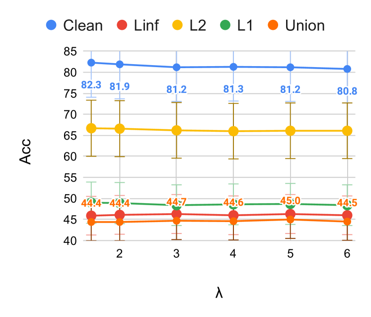
(a) $\lambda$: Robust fine-tuning.

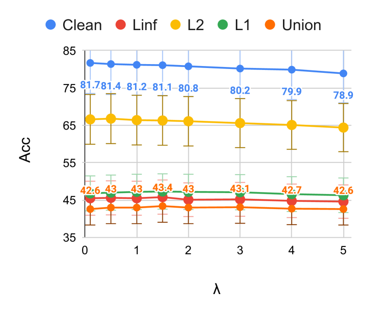
(b) $\lambda$: Training from scratch.

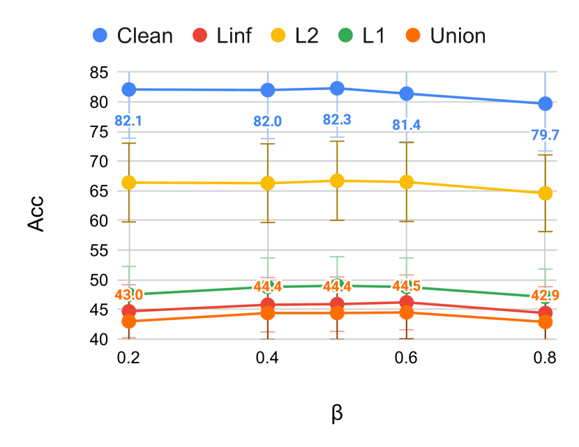
(c) $\beta$: Training from scratch.

Figure 4: Alabtion studies on $\lambda$ and $\beta$ hyper-parameters.

Sensitivities of $\lambda$. We perform experiments with different $\lambda$ values in $[0.1,0.5,1.0,1.5,2,3,4,5]$ for robust fine-tuning and $[1.5,2,3,4,5,6]$ for AT from random initialization using PreAct-ResNet-18 model for CIFAR-10 dataset. In Figure 4, we observe a decreased clean accuracy when $\lambda$ becomes larger. We pick $\lambda=1.5$ for robust fine-tuning (Figure 4(b)) and $\lambda=5.0$ for training from scratch (Figure 4(a)) in our main experiments, as these values of $\lambda$ yield both good clean and union accuracy.

Choices of $\beta$. Figure 4(c) displays the performance of RAMP with varying $\beta$ values on CIFAR-10 ResNet-18 experiments. We pick $\beta=0.5$ as a good middle point for combining natural training and AT via Gradient Projection, which achieves comparatively good robustness and clean accuracy. For bigger $\beta$ values, we incorporate more adversarial training components, which leads to a lower clean accuracy.

Fine-tune $l_{p}$ AT models with RAMP. Table 6 shows the robust fine-tuning results using RAMP with $l_{\infty}$-AT ($q=\infty,r=1$), $l_{1}$-AT ($q=1,r=\infty$), $l_{2}$-AT ($q=\infty,r=1$) RN-18 models for CIRAR-10 dataset. For $l_{\infty}-l_{1}$ tradeoffs, performing RAMP on $l_{\infty}$-AT pre-trained model achieves better union accuracy than $l_{1}$-AT or $l_{2}$-AT pre-trained model.

	Clean	$l_{\infty}$	$l_{2}$	$l_{1}$	Union
RN-18 $l_{\infty}$-AT	80.9	45.5	66.2	47.3	43.1
RN-18 $l_{1}$-AT	78.0	41.5	63.4	46.0	40.4
RN-18 $l_{2}$-AT	83.5	41.9	68.4	45.5	39.7

Table 6: RAMP with $l_{\infty},l_{1},l_{2}$-RN-18-AT models on CIFAR-10.

Fine-tuning with more epochs. In Table 7, we apply robust fine-tuning on the PreAct ResNet-18 model for CIFAR-10 dataset with $5,7,10,15$ epochs, and compared with E-AT. RAMP consistently outperforms the baseline on union accuracy, with a larger improvement when we increase the number of epochs.

	5 epochs		7 epochs		10 epochs		15 epochs
	Clean	Union	Clean	Union	Clean	Union	Clean	Union
E-AT	83.0	43.1	83.1	42.6	84.0	42.8	84.6	43.2
RAMP	81.7	43.6	82.1	43.8	82.5	44.6	83.0	44.9

Table 7: Fine-tuning with more epochs: RAMP consistently outperforms E-AT on union accuracy. E-AT results are from Croce and Hein (2022).

Also, we provide more ablation results applying the trades loss to RAMP in Appendix B.4 using WideResNet-28-10 for CIFAR-10 dataset, where RAMP still outperforms E-AT.

5.4 Discussion

Computational analysis. For AT-GP, the extra natural training costs are small compared with the more expensive AT, e.g. for each epoch on ResNet-18, NT takes $6$ seconds and the standard AT takes $78$ seconds using a single NVIDIA A100 GPU, and the GP operation only takes $0.04$ seconds. Additionally, RAMP has around $2$ times the runtime cost of E-AT and $\frac{2}{3}$ cost of MAX: RAMP, E-AT, and MAX take $157$, $78$, and $219$ seconds per epoch on CIFAR-10 with ResNet-18, respectively.

Limitations. We observe that the clean accuracy sometimes drops when fine-tuning with RAMP. In some cases, union accuracy increases slightly at the cost of decreasing both clean accuracy and single $l_{p}$ robustness. Also, RAMP has a higher time cost than defenses employing random sampling.

6 Conclusion

We present RAMP, a framework that boosts multiple-norm robustness, via alleviating the tradeoffs in robustness among multiple $l_{p}$ perturbations and accuracy/robustness. By analyzing the tradeoffs from the lens of distribution shifts, we identify the key tradeoff pair, apply logit pairing, and leverage gradient projection methods to boost union accuracy with good accuracy/robustness/efficiency tradeoffs. Our results show that RAMP outperforms SOTA methods with better union accuracy, on a wide range of model architectures on CIFAR-10 and ImageNet.

Appendix A Proof of Theorem 1

To prove Theorem 1, we first use the following lemmas from Enyi Jiang [2024], to get the delta errors of Gradient Projection (GP) and standard adversarial training (AT):

Lemma 2 (Delta Error of GP).

Given distributions $\widehat{\mathcal{D}}_{a}$, ${\mathcal{D}}_{a}$ and $\widehat{\mathcal{D}}_{n}$, as well as the model updates $\widehat{g_{a}},g_{a},\widehat{g}_{n}$ on these distributions per epoch, we have $\Delta^{2}_{{GP}}$ as follows

$$\Delta^{2}_{{GP}}\approx\left((1-\beta)^{2}+\frac{2\beta-\beta^{2}}{m}\right)\|g_{a}-\widehat{g}_{n}\|^{2}_{\pi}+\beta^{2}\bar{\tau}^{2}\mathbb{E}_{\widehat{\mathcal{D}}_{a}}\|g_{a}-\widehat{g}_{a}\|^{2}_{\pi},$$ (8)

In the above equation, $m$ is the model dimension and $\bar{\tau}^{2}=\mathbb{E}_{\pi}[\tau^{2}]\in[0,1]$ where $\tau$ is the $\sin(\cdot)$ value of the angle between $\widehat{g}_{n}$ and $g_{a}-\widehat{g}_{n}$. $\|\cdot\|_{\pi}$ is the $\pi$-norm over the model parameter space.

Lemma 3 (Delta Error of AT).

Given distributions $\widehat{\mathcal{D}}_{a}$, ${\mathcal{D}}_{a}$ and $\widehat{\mathcal{D}}_{n}$, as well as the model updates $\widehat{g_{a}},g_{a},\widehat{g}_{n}$ on these distributions per epoch, we have $\Delta^{2}_{AT}$ as follows

$$\Delta^{2}_{AT}=\mathbb{E}_{\widehat{\mathcal{D}}_{a}}\|g_{a}-\widehat{g}_{a}\|^{2}_{\pi},$$ (9)

where $\|\cdot\|_{\pi}$ is the $\pi$-norm over the model parameter space.

Then, we prove Theorem 1.

Theorem 4 (Error Analysis of GP).

When the model dimension is large ($m\rightarrow\infty$), we have

$$\Delta^{2}_{AT}-\Delta^{2}_{GP}\approx\left((1-\beta^{2}\bar{\tau}^{2})\mathbb{E}_{\widehat{\mathcal{D}}_{a}}\|g_{a}-\widehat{g}_{a}\|^{2}_{\pi}-(1-\beta^{2})\|g_{a}-\widehat{g}_{n}\|^{2}_{\pi}\right)+2\beta\|g_{a}-\widehat{g}_{n}\|^{2}_{\pi}$$

$\bar{\tau}^{2}=\mathbb{E}_{\pi}[\tau^{2}]\in[0,1]$ where $\tau$ is the $\sin(\cdot)$ value of the angle between $\widehat{g}_{n}$ and $g_{a}-\widehat{g}_{n}$, $\|\cdot\|_{\pi}$ is the $\pi$-norm over the model parameter space.

Proof.

$$\Delta^{2}_{\texttt{AT}}-\Delta^{2}_{\texttt{GP}}\approx\mathbb{E}_{\widehat{\mathcal{D}}_{a}}\|g_{a}-\widehat{g_{a}}\|^{2}_{\pi}-\left((1-\beta)^{2}+\frac{2\beta-\beta^{2}}{m}\right)\|g_{a}-\widehat{g}_{n}\|^{2}_{\pi}-\beta^{2}\bar{\tau}^{2}\mathbb{E}_{\widehat{\mathcal{D}}_{a}}\|g_{a}-\widehat{g}_{a}\|^{2}_{\pi}$$

$$=(1-\beta^{2}\bar{\tau}^{2})\mathbb{E}_{\widehat{\mathcal{D}}_{a}}\|g_{a}-\widehat{g}_{a}\|^{2}_{\pi}-\left((1-\beta)^{2}+\frac{2\beta-\beta^{2}}{m}\right)\|g_{a}-\widehat{g}_{n}\|^{2}_{\pi}$$

$$=(1-\beta^{2}\bar{\tau}^{2})\mathbb{E}_{\widehat{\mathcal{D}}_{a}}\|g_{a}-\widehat{g}_{a}\|^{2}_{\pi}-(1-\beta)^{2}\|g_{a}-\widehat{g}_{n}\|^{2}_{\pi}-\frac{2\beta-\beta^{2}}{m}\|g_{a}-\widehat{g}_{n}\|^{2}_{\pi}$$

$$=\left((1-\beta^{2}\bar{\tau}^{2})\mathbb{E}_{\widehat{\mathcal{D}}_{a}}\|g_{a}-\widehat{g}_{a}\|^{2}_{\pi}-(1-\beta^{2})\|g_{a}-\widehat{g}_{n}\|^{2}_{\pi}\right)+2\beta\|g_{a}-\widehat{g}_{n}\|^{2}_{\pi}-\frac{2\beta-\beta^{2}}{m}\|g_{a}-\widehat{g}_{n}\|^{2}_{\pi}$$

When $m\rightarrow\infty$, we have a simplified version of the error difference as follows

$$\Delta^{2}_{AT}-\Delta^{2}_{GP}\approx\left((1-\beta^{2}\bar{\tau}^{2})\mathbb{E}_{\widehat{\mathcal{D}}_{a}}\|g_{a}-\widehat{g}_{a}\|^{2}_{\pi}-(1-\beta^{2})\|g_{a}-\widehat{g}_{n}\|^{2}_{\pi}\right)+2\beta\|g_{a}-\widehat{g}_{n}\|^{2}_{\pi}$$

∎

Interpretation. Since $\bar{\tau}^{2}\in[0,1]$, we have $(1-\beta^{2}\bar{\tau}^{2})\geq(1-\beta^{2})$. Thus, when $\mathbb{E}_{\widehat{\mathcal{D}}_{a}}\|g_{a}-\widehat{g}_{a}\|^{2}_{\pi}$ is not so different from $\|g_{a}-\widehat{g}_{n}\|^{2}_{\pi}$, we can always show $\Delta^{2}_{AT}>\Delta^{2}_{GP}$, because of the positive term $2\beta\|g_{a}-\widehat{g}_{n}\|^{2}_{\pi}$ and $(1-\beta^{2}\bar{\tau}^{2})\geq(1-\beta^{2})$.

Appendix B Additional Experiment Information

In this section, we provide more training details, additional ablation studies on different logit pairing losses, and AT from random initialization results on CIFAR-10 using WideResNet-28-10.

B.1 More Training Details

We set the batch size to $128$ for the experiments on ResNet-18 and WideResNet-28-10 architectures. For other experiments on CIFAR-10 and ImageNet, we use a batch size of $64$ to fit into the GPU memory for larger models. For all training procedures, we select the last checkpoint for the comparison. When the pre-trained model was originally trained with extra data beyond the CIFAR-10 dataset, similar to Croce and Hein [2022], we use the extra $500$k images introduced by Carmon et al. [2019] for fine-tuning, and each batch contains the same amount of standard and extra images. An epoch is completed when the whole standard training set has been used.

B.2 Additional Experiments with Different Epsilon Values

In this section, we provide additional results with different $\epsilon_{1},\epsilon_{2},\epsilon_{\infty}$ values. We select $\epsilon_{\infty}=[\frac{2}{255},\frac{4}{255},\frac{12}{255},\frac{16}{255}]$, $\epsilon_{1}=[6,9,12,15]$, and $\epsilon_{2}=[0.25,0.75,1.0,1.5]$. In Section B.2.1, we provide visualizations and analysis of key-off pair changing trends similar to Figure 1. In addition, we provide additional RAMP results compared with related baselines with training from scratch and performing robust fine-tuning in Section B.2.2 and Section B.2.3, respectively. We observe that RAMP can surpass E-AT with significant margins for both training from scratch and robust fine-tuning.

B.2.1 Additional Key Trade-off Pair Visualizations and Trend Analysis

Addition key trade-off pair visualizations and identifications. Figure 5, Figure 6, and Figure 7 display key trade-off pairs with $l_{1},l_{2},l_{\infty}$ AT pre-trained models, using varying $\epsilon_{\infty},\epsilon_{1},\epsilon_{2}$ values respectively. The heuristic we use to identify the key trade-off pair is similar to what we present in the main paper, where we first identify the $l_{p}$ robustness of the $l_{p}$-AT model. After that, we select the perturbation with the lowest robustness becomes the starting point of robust fine-tuning. Also, the key trade-off pair includes two perturbations with lower $l_{p}$ robustness. The insight is that the $l_{p}$ robustness of the $l_{p}$-AT model reveals the strength of the perturbation: the stronger attacks are more inclusive to the weaker ones. We show this heuristic works in most cases with both full training and robust fine-tuning in Section B.2.2 and Section B.2.3.

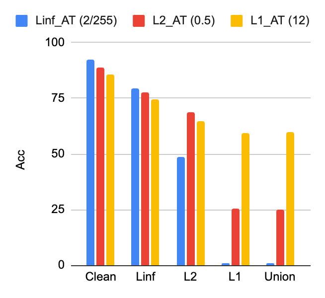
(a) $l_{1}$ - $l_{2}$.

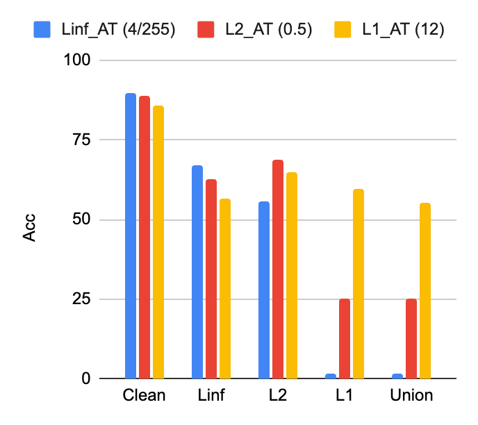
(b) $l_{1}$ - $l_{\infty}$.

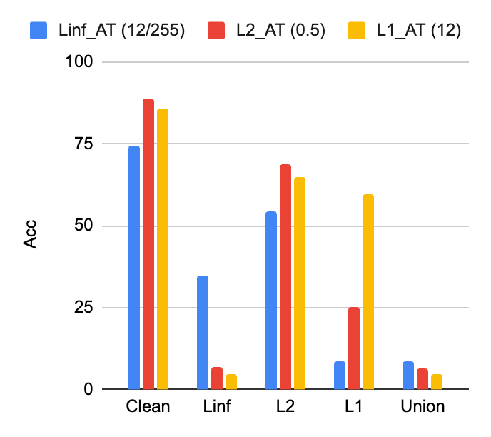
(c) $l_{\infty}$ - $l_{1}$.

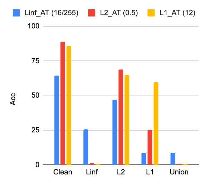
(d) $l_{\infty}$ - $l_{1}$.

Figure 5: Key trade-off pair identifications with $\epsilon_{\infty}=[\frac{2}{255},\frac{4}{255},\frac{12}{255},\frac{16}{255}]$.

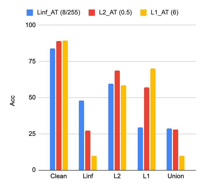
(a) $l_{\infty}$ - $l_{1}$.

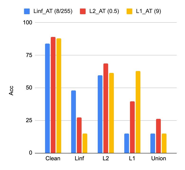
(b) $l_{\infty}$ - $l_{1}$.

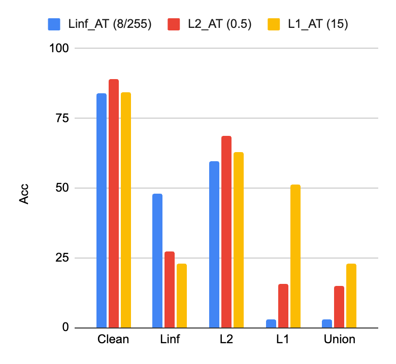
(c) $l_{\infty}$ - $l_{1}$.

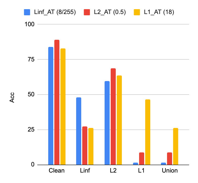
(d) $l_{1}$ - $l_{\infty}$.

Figure 6: Key trade-off pair identifications with $\epsilon_{1}=[6,9,12,15]$.

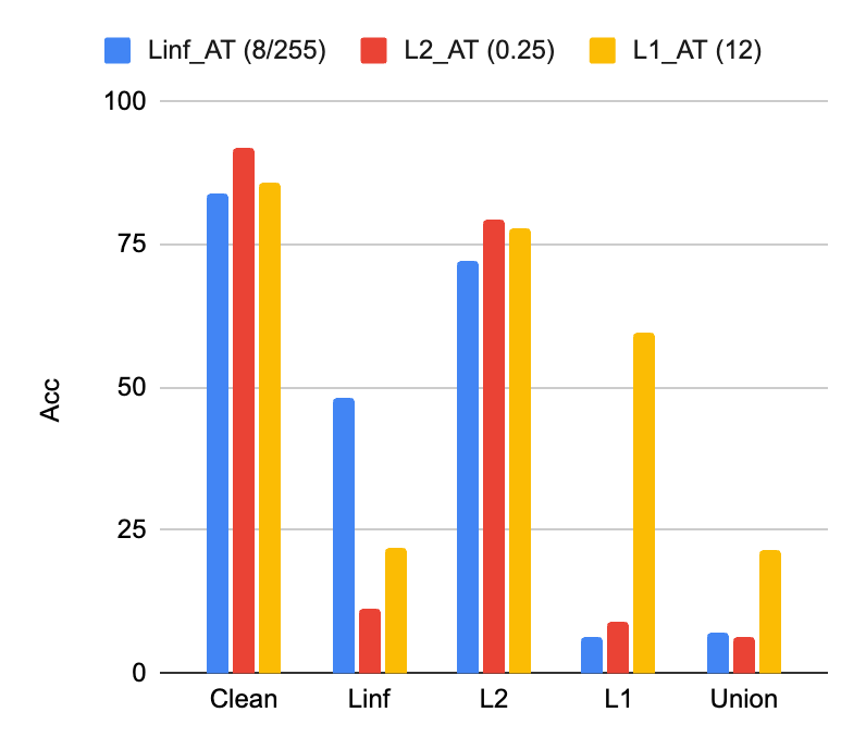
(a) $l_{\infty}$ - $l_{1}$.

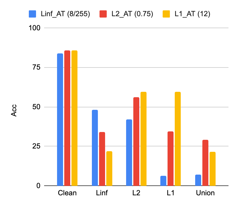
(b) $l_{\infty}$ - $l_{1}$.

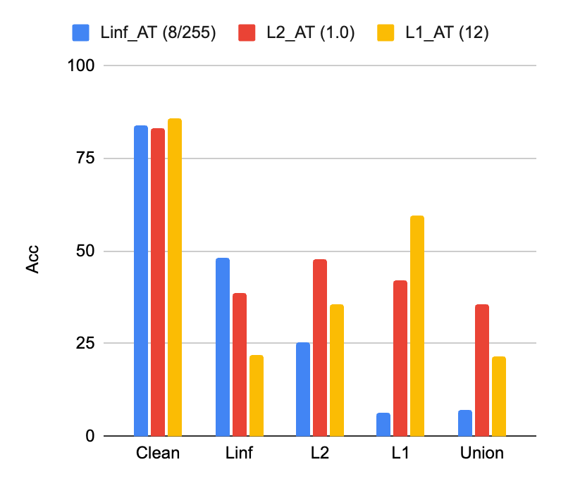
(c) $l_{\infty}$ - $l_{1}$.

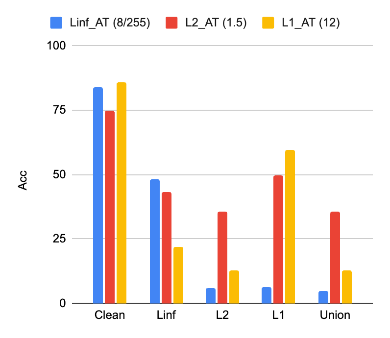
(d) $l_{2}$ - $l_{\infty}$.

Figure 7: Key trade-off pair identifications with $\epsilon_{2}=[0.25,0.75,1.0,1.5]$.

Key tradeoff pair trend analysis. In most cases, $l_{\infty}$ - $l_{1}$ serves as the key tradeoff pair, yet we also observe some special cases when the key tradeoff pair changes, as discussed in the main paper. Here, we provide the trend analysis of varying values of each perturbation type.

• $\mathbf{l_{\infty}}$: $l_{1}$ - $l_{2}$ to $l_{\infty}$ - $l_{1}$. For varying $\epsilon_{\infty}$ values, when $\epsilon_{\infty}$ is small (e.g. $\frac{2}{255}$), $l_{\infty}$ perturbation is removed from the key tradeoff pair because of the high robustness against the $l_{\infty}$-AT model. When increasing $\epsilon_{\infty}$, $l_{\infty}$ robustness of the $l_{\infty}$-AT model decreases but $l_{2}$ robustness of the $l_{2}$-AT model remains relatively high, so $l_{2}$ is removed from the key trade-off pair after some cutoff values.

• $\mathbf{l_{1}}$: $l_{\infty}$ - $l_{1}$ to $l_{1}$ - $l_{\infty}$. Changing $\epsilon_{1}$ values has little effect on $l_{2}$ robustness of all pre-trained models, which makes $l_{2}$ removed in the key trade-off pair all the time. After some cutoff values, the key trade-off pair becomes $l_{1}$ - $l_{\infty}$ since $l_{1}$ robustness of the $l_{1}$-AT model is decreasing and at some point, it becomes lower than $l_{\infty}$ robustness of the $l_{\infty}$-AT model.

• $\mathbf{l_{2}}$: $l_{\infty}$ - $l_{1}$ to $l_{2}$ - $l_{\infty}$. For varying $\epsilon_{2}$ values, when $\epsilon_{2}$ is small (e.g. $0.25,0.75$), $l_{2}$ perturbation is removed from the key tradeoff pair because of the high robustness against the $l_{2}$-AT model. When increasing $\epsilon_{2}$, $l_{2}$ robustness of the $l_{2}$-AT model decreases but $l_{1}$ robustness of the $l_{1}$-AT model remains relatively high, so $l_{1}$ is removed from the key trade-off pair after some cutoff values.

B.2.2 Additional Results with Training from Scratch

Changing $l_{\infty}$ perturbations with $\epsilon_{\infty}=[\frac{2}{255},\frac{4}{255},\frac{12}{255},\frac{16}{255}]$. Table 8 and Table 9 show that RAMP consistently outperforms E-AT [Croce and Hein, 2022] on union accuracy when training from scratch.

Table 8: $(\epsilon_{\infty}=\mathbf{\frac{2}{255}},\epsilon_{1}=12,\epsilon_{2}=0.5)$ and $(\epsilon_{\infty}=\mathbf{\frac{4}{255}},\epsilon_{1}=12,\epsilon_{2}=0.5)$ with random initializations.

	Clean	$l_{\infty}$	$l_{2}$	$l_{1}$	Union
E-AT	87.2	73.3	64.1	55.4	55.4
RAMP	86.4	73.6	65.4	59.8	59.7

	Clean	$l_{\infty}$	$l_{2}$	$l_{1}$	Union
E-AT	86.8	58.9	66.4	54.6	53.7
RAMP	85.7	60.1	67.1	59.1	58.1

Table 9: $(\epsilon_{\infty}=\mathbf{\frac{12}{255}},\epsilon_{1}=12,\epsilon_{2}=0.5)$ and $(\epsilon_{\infty}=\mathbf{\frac{16}{255}},\epsilon_{1}=12,\epsilon_{2}=0.5)$ with random initializations.

	Clean	$l_{\infty}$	$l_{2}$	$l_{1}$	Union
E-AT	77.5	28.8	64.0	50.1	28.7
RAMP	72.2	34.7	57.3	38.9	33.6

	Clean	$l_{\infty}$	$l_{2}$	$l_{1}$	Union
E-AT	69.4	18.8	58.7	47.7	18.7
RAMP	62.8	26.1	48.4	31.7	25.4

Changing $l_{1}$ perturbations with $\epsilon_{1}=[6,9,12,15]$. Table 10 and Table 11 show that RAMP consistently outperforms E-AT [Croce and Hein, 2022] on union accuracy when training from scratch.

Table 10: $(\epsilon_{\infty}=\frac{2}{255},\mathbf{\epsilon_{1}=6},\epsilon_{2}=0.5)$ and $(\epsilon_{\infty}=\frac{4}{255},\mathbf{\epsilon_{1}=9},\epsilon_{2}=0.5)$ with random initializations.

	Clean	$l_{\infty}$	$l_{2}$	$l_{1}$	Union
E-AT	85.5	43.1	67.9	63.9	42.8
RAMP	82.4	48.7	62.0	48.5	45.4

	Clean	$l_{\infty}$	$l_{2}$	$l_{1}$	Union
E-AT	84.6	41.8	67.7	57.6	41.4
RAMP	82.3	47.4	65.0	49.5	45.6

Table 11: $(\epsilon_{\infty}=\frac{12}{255},\mathbf{\epsilon_{1}=15},\epsilon_{2}=0.5)$ and $(\epsilon_{\infty}=\frac{16}{255},\mathbf{\epsilon_{1}=18},\epsilon_{2}=0.5)$ with random initializations.

	Clean	$l_{\infty}$	$l_{2}$	$l_{1}$	Union
E-AT	81.9	40.2	66.9	48.7	39.2
RAMP	79.9	45.3	65.8	47.0	44.0

	Clean	$l_{\infty}$	$l_{2}$	$l_{1}$	Union
E-AT	81.0	39.8	65.8	44.3	38.0
RAMP	79.0	43.8	65.6	44.8	42.1

Changing $l_{2}$ perturbations with $\epsilon_{2}=[0.25,0.75,1.0,1.5]$. Table 12 and Table 13 show that RAMP consistently outperforms E-AT [Croce and Hein, 2022] on union accuracy when training from scratch.

Table 12: $(\epsilon_{\infty}=\frac{2}{255},\epsilon_{1}=12,\mathbf{\epsilon_{2}=0.25})$ and $(\epsilon_{\infty}=\frac{4}{255},\epsilon_{1}=12,\mathbf{\epsilon_{2}=0.75})$ with random initializations.

	Clean	$l_{\infty}$	$l_{2}$	$l_{1}$	Union
E-AT	82.8	41.3	75.6	52.9	40.5
RAMP	81.1	46.5	73.8	48.6	45.1

	Clean	$l_{\infty}$	$l_{2}$	$l_{1}$	Union
E-AT	83.0	41.2	57.6	53.0	40.5
RAMP	81.2	46.3	56.5	48.7	44.9

Table 13: $(\epsilon_{\infty}=\frac{12}{255},\epsilon_{1}=12,\mathbf{\epsilon_{2}=1.0})$ and $(\epsilon_{\infty}=\frac{16}{255},\epsilon_{1}=12,\mathbf{\epsilon_{2}=1.5})$ with random initializations.

	Clean	$l_{\infty}$	$l_{2}$	$l_{1}$	Union
E-AT	83.4	41.0	47.3	52.8	40.3
RAMP	81.5	46.0	46.5	48.1	44.1

	Clean	$l_{\infty}$	$l_{2}$	$l_{1}$	Union
E-AT	83.5	41.0	25.5	52.9	25.5
RAMP	73.7	43.7	37.3	51.6	37.3

B.2.3 Additional Results with Robust Fine-tuning

Changing $l_{\infty}$ perturbations with $\epsilon_{\infty}=[\frac{2}{255},\frac{4}{255},\frac{12}{255},\frac{16}{255}]$. Table 14 and Table 15 show that RAMP consistently outperforms E-AT [Croce and Hein, 2022] on union accuracy when performing robust fine-tuning.

Table 14: $(\epsilon_{\infty}=\mathbf{\frac{2}{255}},\epsilon_{1}=12,\epsilon_{2}=0.5)$ and $(\epsilon_{\infty}=\mathbf{\frac{4}{255}},\epsilon_{1}=12,\epsilon_{2}=0.5)$ with robust fine-tuning.

	Clean	$l_{\infty}$	$l_{2}$	$l_{1}$	Union
E-AT	86.5	74.8	66.7	57.9	57.9
RAMP	85.8	73.5	65.8	60.4	60.3

	Clean	$l_{\infty}$	$l_{2}$	$l_{1}$	Union
E-AT	85.9	61.4	67.9	57.6	56.8
RAMP	85.6	60.9	67.5	59.5	58.4

Table 15: $(\epsilon_{\infty}=\mathbf{\frac{12}{255}},\epsilon_{1}=12,\epsilon_{2}=0.5)$ and $(\epsilon_{\infty}=\mathbf{\frac{16}{255}},\epsilon_{1}=12,\epsilon_{2}=0.5)$ with robust fine-tuning..

	Clean	$l_{\infty}$	$l_{2}$	$l_{1}$	Union
E-AT	75.5	30.8	62.4	44.6	30.0
RAMP	73.6	33.9	59.4	38.0	32.2

	Clean	$l_{\infty}$	$l_{2}$	$l_{1}$	Union
E-AT	68.7	20.7	56.1	42.1	20.5
RAMP	65.3	25.0	50.8	30.8	23.8

Changing $l_{1}$ perturbations with $\epsilon_{1}=[6,9,12,15]$. Table 10 and Table 11 show that RAMP consistently outperforms E-AT [Croce and Hein, 2022] on union accuracy when performing robust fine-tuning.

Table 16: $(\epsilon_{\infty}=\frac{2}{255},\mathbf{\epsilon_{1}=6},\epsilon_{2}=0.5)$ and $(\epsilon_{\infty}=\frac{4}{255},\mathbf{\epsilon_{1}=9},\epsilon_{2}=0.5)$ with robust fine-tuning.

	Clean	$l_{\infty}$	$l_{2}$	$l_{1}$	Union
E-AT	84.2	45.8	66.8	59.0	45.0
RAMP	83.0	48.7	63.5	51.7	46.4

	Clean	$l_{\infty}$	$l_{2}$	$l_{1}$	Union
E-AT	83.1	44.9	67.2	52.6	43.2
RAMP	82.1	47.3	65.7	49.7	44.9

Table 17: $(\epsilon_{\infty}=\frac{12}{255},\mathbf{\epsilon_{1}=15},\epsilon_{2}=0.5)$ and $(\epsilon_{\infty}=\frac{16}{255},\mathbf{\epsilon_{1}=18},\epsilon_{2}=0.5)$ with robust fine-tuning.

	Clean	$l_{\infty}$	$l_{2}$	$l_{1}$	Union
E-AT	81.3	43.5	66.6	42.8	39.0
RAMP	79.7	43.9	66.0	44.7	41.4

	Clean	$l_{\infty}$	$l_{2}$	$l_{1}$	Union
E-AT	81.3	38.9	66.6	45.0	37.5
RAMP	80.0	40.9	66.0	44.0	39.4

Changing $l_{2}$ perturbations with $\epsilon_{2}=[0.25,0.75,1.0,1.5]$. Table 12 and Table 13 show that RAMP consistently outperforms E-AT [Croce and Hein, 2022] on union accuracy when performing robust fine-tuning.

Table 18: $(\epsilon_{\infty}=\frac{2}{255},\epsilon_{1}=12,\mathbf{\epsilon_{2}=0.25})$ and $(\epsilon_{\infty}=\frac{4}{255},\epsilon_{1}=12,\mathbf{\epsilon_{2}=0.75})$ with robust fine-tuning.

	Clean	$l_{\infty}$	$l_{2}$	$l_{1}$	Union
E-AT	82.3	44.2	75.3	47.2	41.4
RAMP	81.2	45.5	73.9	47.1	43.1

	Clean	$l_{\infty}$	$l_{2}$	$l_{1}$	Union
E-AT	83.0	43.5	58.1	46.5	40.4
RAMP	81.0	45.5	57.3	47.3	43.2

Table 19: $(\epsilon_{\infty}=\frac{12}{255},\epsilon_{1}=12,\mathbf{\epsilon_{2}=1.0})$ and $(\epsilon_{\infty}=\frac{16}{255},\epsilon_{1}=12,\mathbf{\epsilon_{2}=1.5})$ with robust fine-tuning.

	Clean	$l_{\infty}$	$l_{2}$	$l_{1}$	Union
E-AT	82.3	41.0	49.0	51.6	40.2
RAMP	81.0	45.5	47.7	47.2	43.1

	Clean	$l_{\infty}$	$l_{2}$	$l_{1}$	Union
E-AT	80.2	42.8	31.5	52.4	31.5
RAMP	74.6	43.5	37.1	50.8	37.0

B.3 Different Logit Pairing Methods

In this section, we test RAMP with robust fine-tuning using two more different logit pairing losses: (1) Mean Squared Error Loss ($\mathcal{L}_{mse}$) (Eq. 10), (2) Cosine-Similarity Loss ($\mathcal{L}_{cos}$) (Eq. 11). We replace the KL loss we used in the paper using the following losses. We use the same lambda value $\lambda=1.5$ for both cases.

$$\mathcal{L}_{mse}=\frac{1}{n_{c}}\cdot\sum^{n_{c}}_{i=0}\frac{1}{2}\left(p_{q}[\gamma[i]]-p_{r}[\gamma[i]]\right)^{2}$$ (10)

$$\mathcal{L}_{cos}=\frac{1}{n_{c}}\cdot\sum^{n_{c}}_{i=0}\left(1-\cos(p_{q}[\gamma[i]],p_{r}[\gamma[i]])\right)$$ (11)

Table 20 displays RAMP robust fine-tuning results of different logit pairing losses using PreAct-ResNet-18 on CIFAR-10. We see those losses generally improve union accuracy compared with baselines in Table 2. $\mathcal{L}_{cos}$ has a better clean accuracy yet slightly worsened union accuracy. $\mathcal{L}_{mse}$ has the best union accuracy and the worst clean accuracy. $\mathcal{L}_{KL}$ is in the middle of the two others. However, we acknowledge the possibility that each logit pairing loss may have its own best-tuned $\lambda$ value.

Losses	Clean	$l_{\infty}$	$l_{2}$	$l_{1}$	Union
KL	80.9	45.5	66.2	47.3	43.1
MSE	80.4	45.6	65.8	47.6	43.5
Cosine	81.6	45.4	66.7	47.0	42.9

Table 20: RAMP fine-tuning results of different logit pairing losses using PreAct-ResNet-18 on CIFAR-10.

B.4 AT from Scratch Using WideResNet-28-10

Implementations. We use a cyclic learning rate with a maximum rate of $0.1$ for $30$ epochs and adopt the outer minimization trades loss from Zhang et al. [2019] with the default hyperparameters, same as Croce and Hein [2022]. Additionally, we use the WideResNet-28-10 architecture same as Zagoruyko and Komodakis [2016] for our reimplementations on CIFAR-10.

Results. Since the implementation of experiments on WideResNet-28-10 in Croce and Hein [2022] paper is not public at present, we report our implementation results on E-AT, where our results show that RAMP outperforms E-AT in union accuracy with a significant margin, as shown in Table 21. Also, we experiment with using the trade loss (RAMP w trades) for the outer minimization, we observe that RAMP w trades achieves a better union accuracy at the loss of some clean accuracy.

Methods	Clean	$l_{\infty}$	$l_{2}$	$l_{1}$	Union
E-AT w trades (reported in [Croce and Hein, 2022])	79.9	46.6	66.2	56.0	46.4
E-AT w trades (ours)	79.2	44.2	64.9	54.9	44.0
RAMP w/o trades (ours)	81.8	46.5	65.5	47.5	44.6
RAMP w trades (ours)	78.0	46.3	63.1	48.6	45.2

Table 21: WideResNet-28-10 trained from random initialization on CIFAR-10. RAMP outperforms E-AT on union accuracy with our implementation.

Appendix C Additional Visualization Results

In this section, we provide additional t-SNE visualizations of the multiple-norm tradeoff and robust fine-tuning procedures using different methods.

C.1 Pre-trained $l_{1},l_{2},l_{\infty}$ AT models

Figure 8 shows the robust accuracy of $l_{1},l_{2},l_{\infty}$ AT models against their respect $l_{1},l_{2},l_{\infty}$ perturbations, on CIFAR-10 using PreAct-ResNet-18 architecture. Similar to Figure 1(b), $l_{\infty}$-AT model has a low $l_{1}$ robustness and vice versa. In this common choice of epsilons, we further confirm that $l_{\infty}-l_{1}$ is the key trade-off pair.

C.2 Robust Fine-tuning for all Epochs

We provide the complete visualizations of robust fine-tuning for 3 epochs on CIFAR-10 using $l_{1}$ examples, E-AT, and RAMP. Rows in $l_{1}$ fine-tuning (Figure 9), E-AT fine-tuning (Figure 10), and RAMP fine-tuning (Figure 11) show the robust accuracy against $l_{\infty},l_{1},l_{2}$ attacks individually, of epoch $0,1,2,3$, respectively. We observe that throughout the procedure, RAMP manages to maintain more $l_{\infty}$ robustness during the fine-tuning with more points colored in cyan, in comparison with two other methods. This visualization confirms that after we identify a $l_{p}-l_{r}(p\neq r)$ key tradeoff pair, RAMP successfully preserves more $l_{p}$ robustness when training with some $l_{r}$ examples via enforcing union predictions with the logit pairing loss.

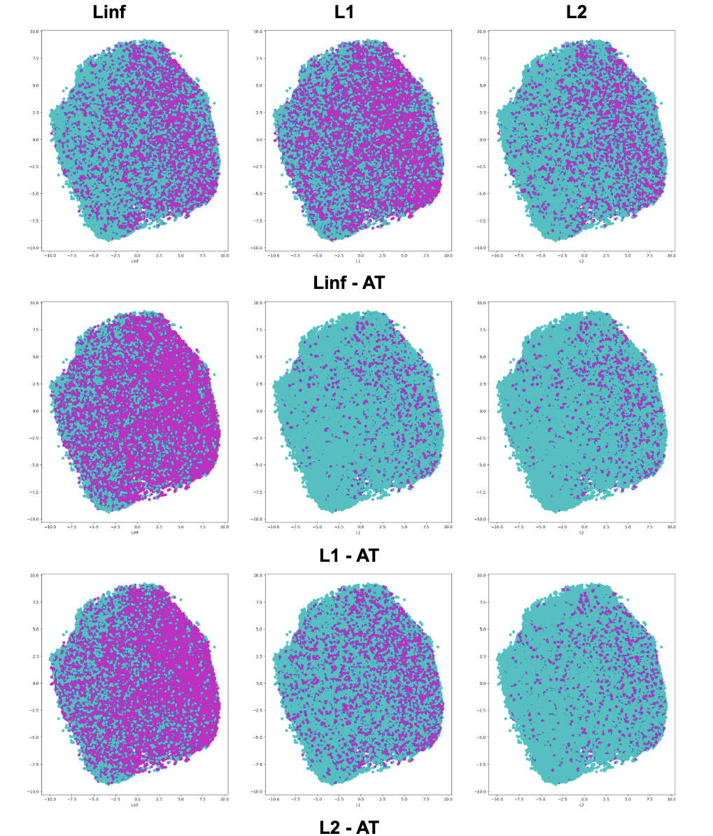
Figure 8: $l_{1},l_{2},l_{\infty}$ pre-trained RN18 $l_{\infty}$-AT models with correct/incorrect predictions against $l_{1},l_{2},l_{\infty}$ attacks. Correct predictions are colored with cyan and incorrect with magenta. Each row represents $l_{\infty},l_{1},l_{2}$ AT models, respectively. Each column shows the accuracy concerning a certain $l_{p}$ attack.

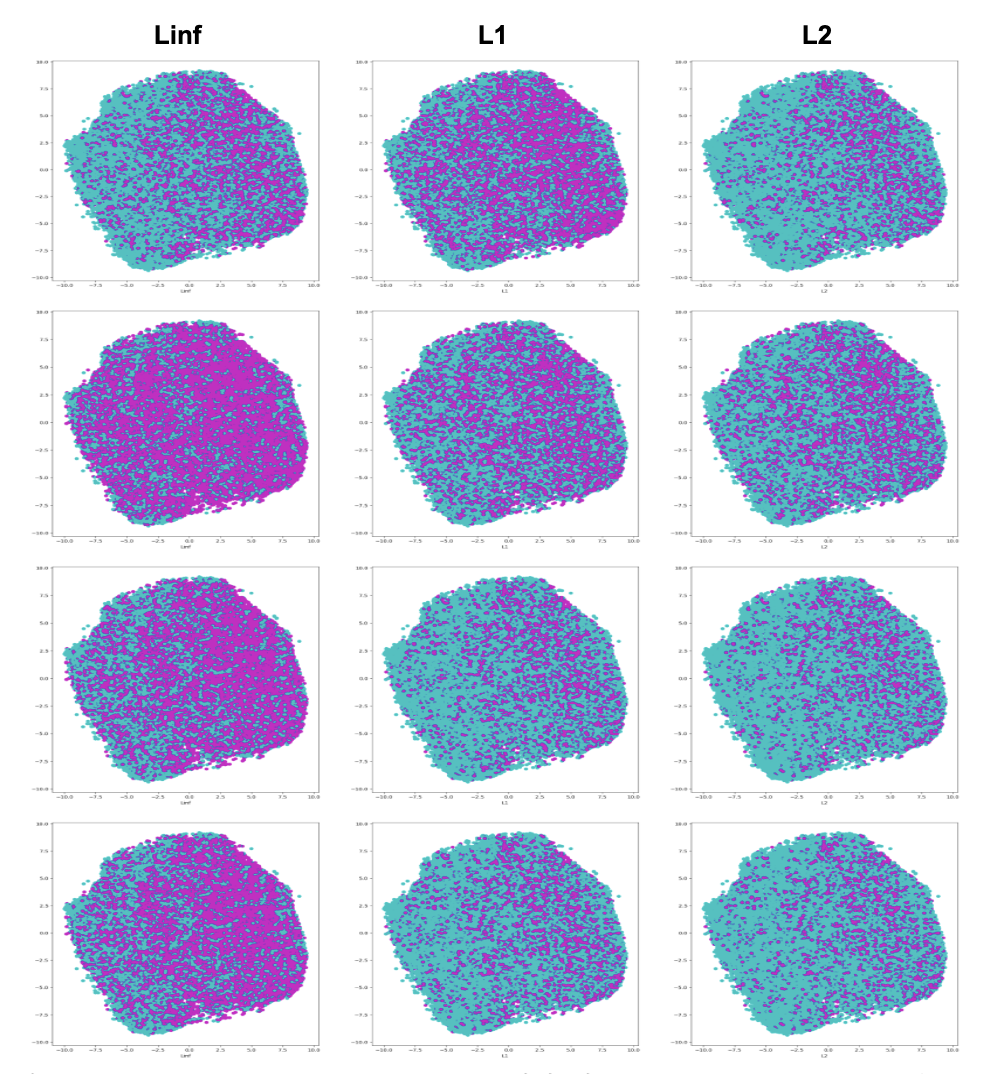
Figure 9: Finetune RN18 $l_{\infty}$-AT model on $l_{1}$ examples for 3 epochs. Each row represents the prediction results of epoch $0,1,2,3$ respectively.

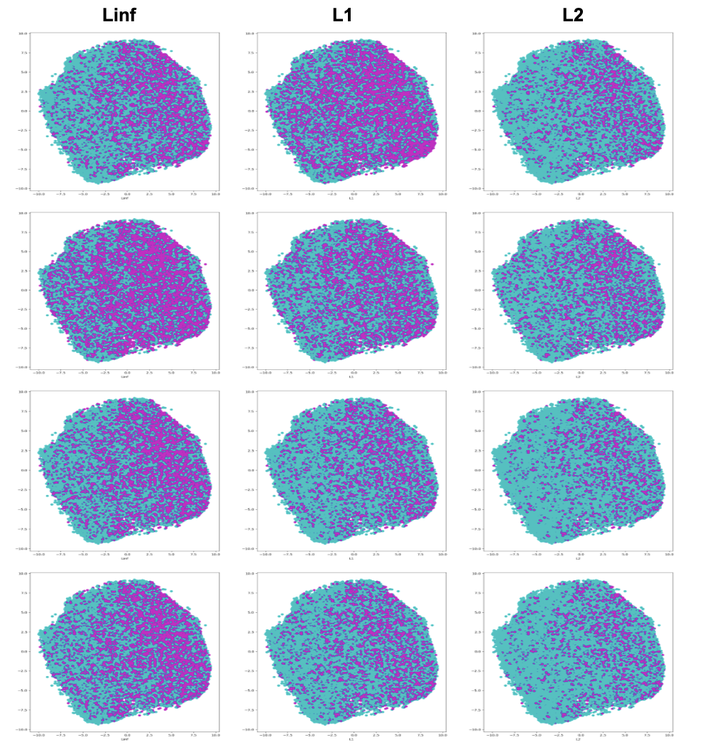
Figure 10: Finetune RN18 $l_{\infty}$-AT model with E-AT for 3 epochs. Each row represents the prediction results of epoch $0,1,2,3$ respectively.

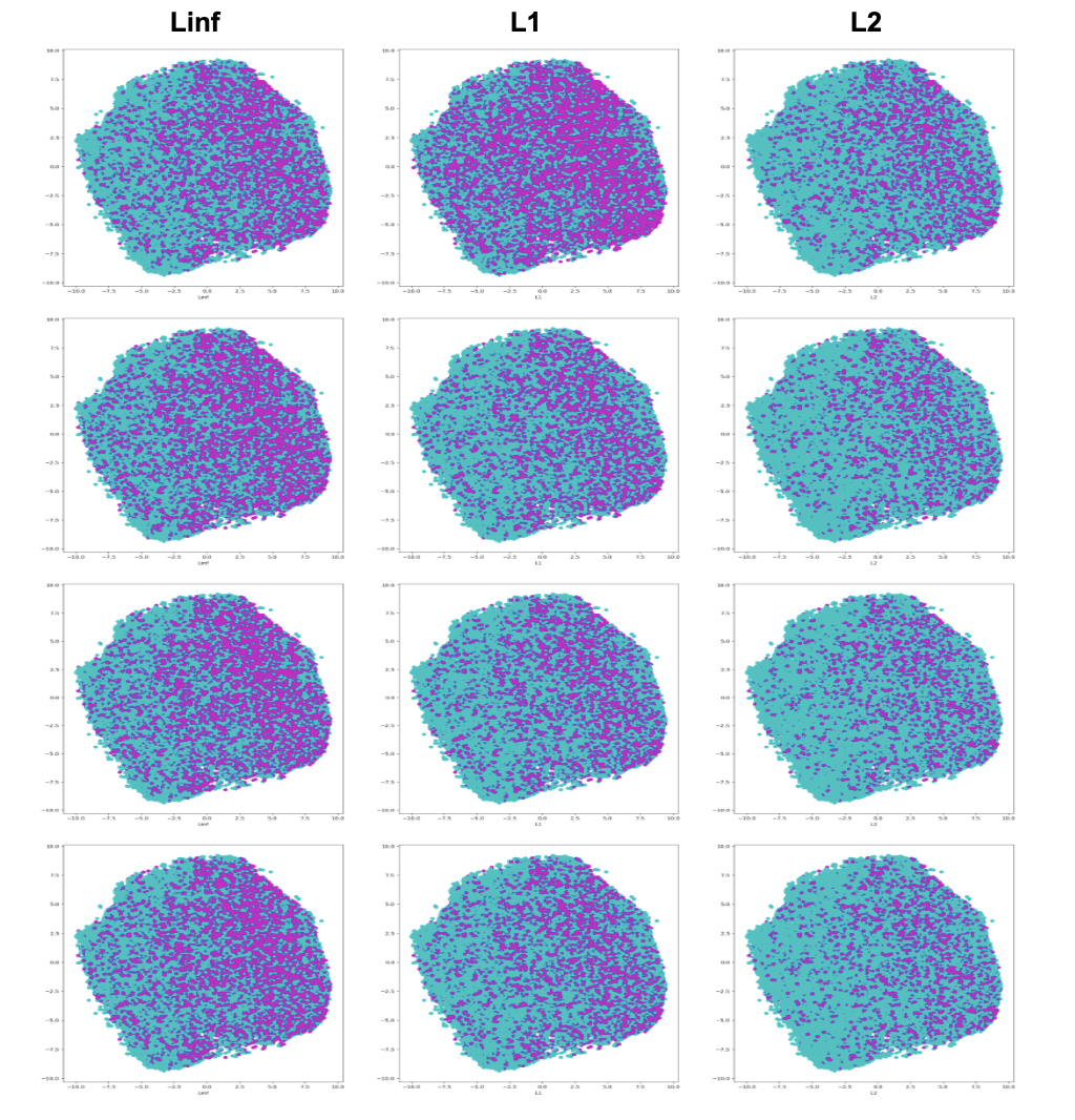
Figure 11: Finetune RN18 $l_{\infty}$-AT model with RAMP for 3 epochs. Each row represents the prediction results of epoch $0,1,2,3$ respectively.

References

- Goodfellow et al. [2014] Ian J Goodfellow, Jonathon Shlens, and Christian Szegedy. Explaining and harnessing adversarial examples. arXiv preprint arXiv:1412.6572, 2014.
- Kurakin et al. [2018] Alexey Kurakin, Ian J Goodfellow, and Samy Bengio. Adversarial examples in the physical world. In Artificial intelligence safety and security, pages 99–112. Chapman and Hall/CRC, 2018.
- Tramèr et al. [2017] Florian Tramèr, Alexey Kurakin, Nicolas Papernot, Ian Goodfellow, Dan Boneh, and Patrick McDaniel. Ensemble adversarial training: Attacks and defenses. arXiv preprint arXiv:1705.07204, 2017.
- Madry et al. [2017] Aleksander Madry, Aleksandar Makelov, Ludwig Schmidt, Dimitris Tsipras, and Adrian Vladu. Towards deep learning models resistant to adversarial attacks. arXiv preprint arXiv:1706.06083, 2017.
- Wang et al. [2020] Yisen Wang, Difan Zou, Jinfeng Yi, James Bailey, Xingjun Ma, and Quanquan Gu. Improving adversarial robustness requires revisiting misclassified examples. In ICLR, 2020.
- Wu et al. [2020] Dongxian Wu, Shu-Tao Xia, and Yisen Wang. Adversarial weight perturbation helps robust generalization. Advances in Neural Information Processing Systems, 33:2958–2969, 2020.
- Carmon et al. [2019] Yair Carmon, Aditi Raghunathan, Ludwig Schmidt, John C Duchi, and Percy S Liang. Unlabeled data improves adversarial robustness. Advances in neural information processing systems, 32, 2019.
- Gowal et al. [2020] Sven Gowal, Chongli Qin, Jonathan Uesato, Timothy Mann, and Pushmeet Kohli. Uncovering the limits of adversarial training against norm-bounded adversarial examples. arXiv preprint arXiv:2010.03593, 2020.
- Raghunathan et al. [2020] Aditi Raghunathan, Sang Michael Xie, Fanny Yang, John Duchi, and Percy Liang. Understanding and mitigating the tradeoff between robustness and accuracy. arXiv preprint arXiv:2002.10716, 2020.
- Zhang et al. [2021] Jingfeng Zhang, Jianing Zhu, Gang Niu, Bo Han, Masashi Sugiyama, and Mohan Kankanhalli. Geometry-aware instance-reweighted adversarial training. In International Conference on Learning Representations, 2021. URL https://openreview.net/forum?id=iAX0l6Cz8ub.
- Debenedetti and Troncoso—EPFL [2022] Edoardo Debenedetti and Carmela Troncoso—EPFL. Adversarially robust vision transformers, 2022.
- Peng et al. [2023] ShengYun Peng, Weilin Xu, Cory Cornelius, Matthew Hull, Kevin Li, Rahul Duggal, Mansi Phute, Jason Martin, and Duen Horng Chau. Robust principles: Architectural design principles for adversarially robust cnns. arXiv preprint arXiv:2308.16258, 2023.
- Wang et al. [2023] Zekai Wang, Tianyu Pang, Chao Du, Min Lin, Weiwei Liu, and Shuicheng Yan. Better diffusion models further improve adversarial training. In Andreas Krause, Emma Brunskill, Kyunghyun Cho, Barbara Engelhardt, Sivan Sabato, and Jonathan Scarlett, editors, Proceedings of the 40th International Conference on Machine Learning, volume 202 of Proceedings of Machine Learning Research, pages 36246–36263. PMLR, 23–29 Jul 2023. URL https://proceedings.mlr.press/v202/wang23ad.html.
- Croce et al. [2020] Francesco Croce, Maksym Andriushchenko, Vikash Sehwag, Edoardo Debenedetti, Nicolas Flammarion, Mung Chiang, Prateek Mittal, and Matthias Hein. Robustbench: a standardized adversarial robustness benchmark. arXiv preprint arXiv:2010.09670, 2020.
- Tramer and Boneh [2019] Florian Tramer and Dan Boneh. Adversarial training and robustness for multiple perturbations. Advances in neural information processing systems, 32, 2019.
- Zhang et al. [2019] Hongyang Zhang, Yaodong Yu, Jiantao Jiao, Eric Xing, Laurent El Ghaoui, and Michael Jordan. Theoretically principled trade-off between robustness and accuracy. In International conference on machine learning, pages 7472–7482. PMLR, 2019.
- Xie et al. [2020] Cihang Xie, Mingxing Tan, Boqing Gong, Jiang Wang, Alan L Yuille, and Quoc V Le. Adversarial examples improve image recognition. In Proceedings of the IEEE/CVF conference on computer vision and pattern recognition, pages 819–828, 2020.
- Benz et al. [2021] Philipp Benz, Chaoning Zhang, and In So Kweon. Batch normalization increases adversarial vulnerability and decreases adversarial transferability: A non-robust feature perspective. In Proceedings of the IEEE/CVF International Conference on Computer Vision, pages 7818–7827, 2021.
- Engstrom et al. [2018] Logan Engstrom, Andrew Ilyas, and Anish Athalye. Evaluating and understanding the robustness of adversarial logit pairing. arXiv preprint arXiv:1807.10272, 2018.
- Jiang et al. [2023] Enyi Jiang, Yibo Jacky Zhang, and Oluwasanmi Koyejo. Federated domain adaptation via gradient projection. arXiv preprint arXiv:2302.05049, 2023.
- Croce and Hein [2022] Francesco Croce and Matthias Hein. Adversarial robustness against multiple and single -threat models via quick fine-tuning of robust classifiers. In International Conference on Machine Learning, pages 4436–4454. PMLR, 2022.
- Kang et al. [2019] Daniel Kang, Yi Sun, Tom Brown, Dan Hendrycks, and Jacob Steinhardt. Transfer of adversarial robustness between perturbation types. arXiv preprint arXiv:1905.01034, 2019.
- Maini et al. [2020] Pratyush Maini, Eric Wong, and Zico Kolter. Adversarial robustness against the union of multiple perturbation models. In International Conference on Machine Learning, pages 6640–6650. PMLR, 2020.
- Madaan et al. [2021] Divyam Madaan, Jinwoo Shin, and Sung Ju Hwang. Learning to generate noise for multi-attack robustness. In International Conference on Machine Learning, pages 7279–7289. PMLR, 2021.
- Kannan et al. [2018] Harini Kannan, Alexey Kurakin, and Ian Goodfellow. Adversarial logit pairing. arXiv preprint arXiv:1803.06373, 2018.
- Sinha et al. [2018] Aman Sinha, Hongseok Namkoong, and John Duchi. Certifiable distributional robustness with principled adversarial training. In International Conference on Learning Representations, 2018. URL https://openreview.net/forum?id=Hk6kPgZA-.
- Moayeri et al. [2022] Mazda Moayeri, Kiarash Banihashem, and Soheil Feizi. Explicit tradeoffs between adversarial and natural distributional robustness. Advances in Neural Information Processing Systems, 35:38761–38774, 2022.
- Alhamoud et al. [2023] Kumail Alhamoud, Hasan Abed Al Kader Hammoud, Motasem Alfarra, and Bernard Ghanem. Generalizability of adversarial robustness under distribution shifts. Transactions on Machine Learning Research, 2023. ISSN 2835-8856. URL https://openreview.net/forum?id=XNFo3dQiCJ. Featured Certification.
- Yang et al. [2020] Yao-Yuan Yang, Cyrus Rashtchian, Hongyang Zhang, Russ R Salakhutdinov, and Kamalika Chaudhuri. A closer look at accuracy vs. robustness. Advances in neural information processing systems, 33:8588–8601, 2020.
- Rade and Moosavi-Dezfooli [2021] Rahul Rade and Seyed-Mohsen Moosavi-Dezfooli. Reducing excessive margin to achieve a better accuracy vs. robustness trade-off. In International Conference on Learning Representations, 2021.
- Jiang [2023] Enyi Jiang. Federated domain adaptation for healthcare, 2023.
- Croce and Hein [2020] Francesco Croce and Matthias Hein. Reliable evaluation of adversarial robustness with an ensemble of diverse parameter-free attacks. In International conference on machine learning, pages 2206–2216. PMLR, 2020.
- Engstrom et al. [2019] Logan Engstrom, Andrew Ilyas, Hadi Salman, Shibani Santurkar, and Dimitris Tsipras. Robustness (python library), 2019. URL https://github.com/MadryLab/robustness.
- Krizhevsky et al. [2009] Alex Krizhevsky, Geoffrey Hinton, et al. Learning multiple layers of features from tiny images. 2009.
- Deng et al. [2009] Jia Deng, Wei Dong, Richard Socher, Li-Jia Li, Kai Li, and Li Fei-Fei. Imagenet: A large-scale hierarchical image database. In 2009 IEEE conference on computer vision and pattern recognition, pages 248–255. Ieee, 2009.
- Russakovsky et al. [2015] Olga Russakovsky, Jia Deng, Hao Su, Jonathan Krause, Sanjeev Satheesh, Sean Ma, Zhiheng Huang, Andrej Karpathy, Aditya Khosla, Michael Bernstein, et al. Imagenet large scale visual recognition challenge. International journal of computer vision, 115:211–252, 2015.
- He et al. [2016] Kaiming He, Xiangyu Zhang, Shaoqing Ren, and Jian Sun. Deep residual learning for image recognition. In Proceedings of the IEEE conference on computer vision and pattern recognition, pages 770–778, 2016.
- Enyi Jiang [2024] Sanmi Koyejo Enyi Jiang, Yibo Jacky Zhang. Principled federated domain adaptation: Gradient projection and auto-weighting. In The Twelfth International Conference on Learning Representations, 2024. URL https://openreview.net/forum?id=6J3ehSUrMU.
- Zagoruyko and Komodakis [2016] Sergey Zagoruyko and Nikos Komodakis. Wide residual networks. In Procedings of the British Machine Vision Conference 2016. British Machine Vision Association, 2016.