Linear response theory for light dark matter-electron scattering in materials

Abstract

We combine the non-relativistic effective theory of dark matter (DM) - electron interactions with linear response theory to obtain a formalism that fully accounts for screening and collective excitations in DM-induced electronic transition rate calculations for general DM-electron interactions. In the same way that the response of a dielectric material to an external electric field in electrodynamics is described by the dielectric function, so in our formalism the response of a detector material to a DM perturbation is described by a set of generalised susceptibilities which can be directly related to densities and currents arising from the non-relativistic expansion of the Dirac Hamiltonian. We apply our formalism to assess the sensitivity of non-spin-polarised detectors, and find that in-medium effects significantly affect the experimental sensitivity if DM couples to the detector’s electron density, while being decoupled from other densities and currents. Our formalism can be straightforwardly extended to the case of spin-polarised materials.

I Introduction

The particles forming our Milky Way dark matter (DM) halo have so far stubbornly escaped detection. A simple hypothesis that could explain this lack of detection is that the DM particle is lighter than the nucleons bound to atomic nuclei, and therefore too light to be directly detected with conventional methods based on the observation of rare nuclear recoils Essig et al. (2012). Indeed, an observable elastic nuclear recoil would require the incoming DM particle to carry a kinetic energy of a few keV or so, and thus to have a mass that lies above the 1 GeV threshold Schumann (2019). This hypothesis motivates the search for DM in electronic transitions induced by the scattering of Milky Way DM particles in detector materials, as these can be triggered by smaller energy depositions than nuclear recoils Mitridate et al. (2023).

Recent experimental proposals for the detection of DM particles with mass in the MeV to GeV range include the search for atomic ionisations in noble gas xenon and argon detectors Essig et al. (2012, 2017); Agnes et al. (2018); Catena et al. (2020); Aprile et al. (2019, 2020) and for electronic transitions in semiconductor crystals Graham et al. (2012); Essig et al. (2016); Derenzo et al. (2017); Agnese et al. (2018); Kurinsky et al. (2019); Aguilar-Arevalo et al. (2019); Arnaud et al. (2020); Barak et al. (2020); Griffin et al. (2021a); Catena et al. (2021); Griffin et al. (2021b); Knapen et al. (2021); Hochberg et al. (2021a); Lasenby and Prabhu (2022); Chen et al. (2022) as well as in superconductors Hochberg et al. (2016, 2021b) and 3D Dirac materials Hochberg et al. (2018); Geilhufe et al. (2019); Coskuner et al. (2021). They also include the search for electron ejections from graphene layers Hochberg et al. (2017); Catena et al. (2023a) and carbon nanotubes Cavoto et al. (2020); Catena et al. (2023b), as well as for excitations of collective phenomena such as phonons Knapen et al. (2018); Trickle et al. (2020a) and magnons Trickle et al. (2020b). Further examples can be found in e.g. Kahn and Lin (2022); Mitridate et al. (2023).

The standard theoretical framework for assessing the potential of these proposals is the dark photon model, where the DM candidate, typically a spin 0 or 1/2 particle, couples to the electrically charged fermions of the Standard Model through the exchange of a “heavy” or “light” spin-1 mediator particle (i.e. the dark photon) Fayet (1980); Holdom (1986); Boehm and Fayet (2004); Fayet (2004); Battaglieri et al. (2017). In this context, a mediator is heavy (light) if the typical momentum transfer in a non-relativistic DM-electron scattering event is much smaller (larger) than its mass. Within this framework, a critical theoretical input to the predicted rate of electronic transitions induced by the scattering of DM particles by the electrons bound to a given material is the overlap integral between the initial and final electron wave functions. In the standard treatment of DM-induced atomic ionisations, the modulus squared of this integral is called the atomic or ionisation form factor, and has been computed using non-relativistic single-particle atomic wave functions Kopp et al. (2009), as well as accounting for many-body Pandey et al. (2018) and relativistic corrections Roberts et al. (2016). In the case of DM-induced electronic transitions from the valence to the conduction band in crystals, the modulus squared of this overlap integral is called the crystal form factor, and has been computed in density functional theory (DFT) by expanding the Bloch states describing electrons in a crystal lattice in plane waves Essig et al. (2016), in an atom-centered gaussian basis Dreyer et al. (2023), or by combining plane waves with atomic orbitals to capture higher momentum contributions Griffin et al. (2021c).

An important observation that has been made recently is that, within the dark photon model, the rate of DM-induced electronic transitions in dielectric materials can be expressed in terms of the underlying dielectric function Hochberg et al. (2021a); Knapen et al. (2021), i.e. the linear response of a dielectric to an external electric field. While the atomic/crystal form factor and dielectric function formalisms are in principle equivalent, the latter allows one to directly account for screening and collective excitation effects which would otherwise be missed by the former when electrons are described using a basis of single-particle states, and in-medium electron-electron interactions are neglected. Notice that screening occurs when the electron density in the target material rearranges itself to partially cancel out the DM-electron interaction. On the other hand, collective excitations occur when the momentum transferred from the DM particle to the medium is smaller than the inverse spacing between separate nuclei, or separate electrons, and the DM particle interacts with multiple particles in the target.

Going beyond the dark photon model, a variety of products of electron wave function overlap integrals can in principle contribute to the rate of DM-induced electronic transitions in materials. We have proven this statement in a recent series of works Catena et al. (2023a, b, c, 2021, 2020), where we have used effective field theory (EFT) methods to describe the interaction between DM and electrons in materials. EFT is a powerful method to address multi-scale physics problems involving a finite set of relevant degrees of freedom and known symmetries. In the case of DM-electron scattering, there is a first separation of scales between the small momentum transfer in the scattering and the electron mass, and a second one between the non-relativistic DM speed in the Milky Way and the speed of light. The relevant degrees of freedom are the DM particle and the electron, while their interactions are constrained by Galilean invariance, and momentum and energy conservation. Combining these building blocks, EFT methods allowed us to write the amplitude for DM-electron scattering as a power series in the small momentum transfer to electron mass ratio, and DM speed to speed of light ratio. This amplitude can describe virtually any model for sub-GeV DM in terms of a finite set of $S-$matrix elements.

Exploiting our EFT approach to DM-electron interactions, we have found that up to seven products of overlap integrals can appear in electron transition rate calculations. These reduce to five in the case of crystals and within a simplified treatment of the local DM velocity distribution Catena et al. (2021). They further reduce to four in the case of isolated atoms Catena et al. (2020), and to one when the final state electron is described by a plane wave Catena et al. (2023a, b). While the framework we have developed in Catena et al. (2023a, b, c, 2021, 2020) allows a rigorous description of previously intractable DM models, such as models where DM has an anapole or a magnetic dipole moment, it does not account for the aforementioned screening and collective excitation effects, as it does not include the many-body response of the remaining electrons to an electronic transition between two bound states.  This makes it impossible to assess whether “in-medium effects” are important in the case of general DM-electron interactions. Furthermore, it prevents us from properly modelling them in cases where they are actually significant.

The main purpose of this work is to extend the dielectric function formalism to the case of general DM-electron interactions in materials. This will enable us to account for in-medium effects in theories beyond the dark photon model. We achieve this goal through the following steps:

1. We start by identifying the electron densities and currents that a spin-1/2 DM particle can couple to in a material. In the dark photon model, DM couples to the electron number density only. In the case of general DM-electron interactions, we find that DM can couple to the electron number density, the paramagnetic current, the spin current, the scalar product of spin and paramagnetic current, and the Rashba spin-orbit current. We then write down the time-dependent potential, $V_{\rm eff}^{ss^{\prime}}(t)$ in Eq. (42), which describes the scattering of DM particles by the bound electrons in any solid-state system in terms of these five densities and currents.

2. We apply linear response theory to calculate the response of a given material to the external, time dependent DM perturbation described by the potential $V_{\rm eff}^{ss^{\prime}}(t)$. As in electrodynamics the response of a dielectric material to an external electric field is described by the dielectric function, so in our formalism the response of a detector material to a DM perturbation is described by a set of generalised susceptibilities. These susceptibilities are associated with the above densities and currents.

3. Using Fermi’s golden rule, we express the rate of DM-induced electronic transitions in detector materials in terms of our set of generalised susceptibilities.

4. We derive and solve a time-evolution equation for the generalised susceptibilities describing the response of a generic solid-state system to an external DM perturbation. Focusing on non-spin-polarised and nearly isotropic materials, we evaluate the solution to this equation, and interpret it diagrammatically.

5. Combing the results from point 3) and point 4) above, we apply our formalism to reassess the sensitivity of hypothetical silicon and germanium detectors.

The linear response theory for light DM direct detection we develop in this work enables us to study the impact of in-medium effects on electronic transition rate calculations in the presence of general DM-electron interactions. Furthermore, it provides us with a framework where we can disentangle in a neat manner the solid state physics contribution, encoded in a set of generalised susceptibilities, from the astro- and particle physics inputs to the rate of DM-induced electronic excitations in materials. While in this work we focus on materials used in existing detectors, our framework can straightforwardly be extended to the case of anisotropic materials, as well as to the case of spin-polarised detectors.

This work is organised as follows. In Sec. II, we identify the densities and currents that DM can couple to in a material. In Sec. III we apply linear response theory to obtain the set of generalised susceptibilities describing the response of a solid-state system to a DM perturbation that couples to the aforementioned densities and currents. We also provide an explicit expression for the rate of DM-induced electronic transitions in materials as a function of our generalised susceptibilities. In Sec. IV we derive and solve a time-evolution equation for the generalised susceptibilities identified in Sec. III. This equation enables us to perform explicit electronic transition rate calculations in the presence of general DM-electron interactions. We apply our formalism to a sample of DM direct detection experiments in Sec. VI and conclude in Sec. VII.

II Dark matter-electron scattering in materials

II.1 Free scattering amplitude in effective theories

In the non-relativistic effective theory of DM-electron interactions Catena et al. (2020), the amplitude for DM scattering by a free electron, $\mathcal{M}$, can be expressed in terms of the DM particle and electron spin operators, $\mathbf{S}_{\chi}$ and $\mathbf{S}_{e}$, respectively, the momentum transfer $\mathbf{q}$ and the transverse relative velocity $\mathbf{v}_{\rm el}^{\perp}$, i.e. the component of the relative DM-electron velocity that is perpendicular to $\mathbf{q}$ when the scattering is elastic

$$\mathbf{v}_{\rm el}^{\perp}\equiv\mathbf{v}^{\perp}_{\chi}+\mathbf{v}^{\perp}_{e}\equiv\left(\frac{\mathbf{p}+\mathbf{p}^{\prime}}{2m_{\chi}}\right)-\left(\frac{\mathbf{k}+\mathbf{k}^{\prime}}{2m_{e}}\right)\,.$$ (1)

Here $\mathbf{k}$ ($\mathbf{k}^{\prime}$) is the initial (final) electron momentum, while $\mathbf{p}$ ($\mathbf{p}^{\prime}$) is the momentum of the incoming (outgoing) DM particle. The electron mass and DM particle mass are denoted by $m_{e}$ and $m_{\chi}$, respectively. In the case of spin-1/2 DM, $\mathbf{S}_{\chi}=\boldsymbol{\sigma}_{\chi}/2$ and $\mathbf{S}_{e}=\boldsymbol{\sigma}_{e}/2$, where the components of the three-dimensional vectors $\boldsymbol{\sigma}_{\chi}$ and $\boldsymbol{\sigma}_{e}$ consist of the three Pauli matrices, and the indexes $\chi$ and $e$ identify the DM particle or electron spin, respectively. For this choice of DM particle spin, and to first order in $\mathbf{v}_{\rm el}^{\perp}$, the amplitude for non-relativistic DM-electron scattering is Catena et al. (2020)

$$\mathcal{M}=\sum_{i}\left(c_{i}^{s}+c^{\ell}_{i}\frac{q_{\rm ref}^{2}}{|\mathbf{q}|^{2}}\right)\,\langle\mathcal{O}_{i}\rangle\,,$$ (2)

where the interaction operators $\mathcal{O}_{i}$ are defined in Tab. 1, and $q_{\rm ref}\equiv\alpha m_{e}$ is a reference momentum, with $\alpha$ the fine structure constant. We denote the coupling constants of the $i$-th operator in Tab. 1 by $c_{i}^{s}$ and $c_{i}^{\ell}$, where $c^{s}_{i}\neq 0$ and $c^{\ell}_{i}=0$ corresponds to the case of interactions mediated by a heavy particle, while $c^{s}_{i}=0$ and $c^{\ell}_{i}\neq 0$ refers to the case of a light mediator. Angle brackets in the amplitude $\mathcal{M}$ denote matrix elements between the two-component spinors $\xi^{s}$ and $\xi^{s^{\prime}}$ for the DM particle, and $\xi^{r}$ and $\xi^{r^{\prime}}$ for the electron. For example, in the case of $\mathcal{O}_{4}$,

$$\langle\mathcal{O}_{4}\rangle\equiv\xi^{s^{\prime}\dagger}\frac{\boldsymbol{\sigma}_{\chi}}{2}\xi^{s}\xi^{r^{\prime}\dagger}\frac{\boldsymbol{\sigma}_{e}}{2}\xi^{r}\,.$$ (3)

By promoting the coupling constants $c^{s}_{i}$ and $c^{\ell}_{i}$ to functions of the momentum transfer, virtually any model for DM-electron interactions can be matched onto the free scattering amplitude in Eq. (2) in the non-relativistic limit.

$\mathcal{O}_{1}=\mathds{1}_{\chi}\mathds{1}_{e}$	$\mathcal{O}_{9}=i\mathbf{S}_{\chi}\cdot\left(\mathbf{S}_{e}\times\frac{\mathbf{q}}{m_{e}}\right)$
$\mathcal{O}_{3}=i\mathbf{S}_{e}\cdot\left(\frac{\mathbf{q}}{m_{e}}\times\mathbf{v}^{\perp}_{\rm el}\right)\mathds{1}_{\chi}$	$\mathcal{O}_{10}=i\mathbf{S}_{e}\cdot\frac{\mathbf{q}}{m_{e}}\mathds{1}_{\chi}$
$\mathcal{O}_{4}=\mathbf{S}_{\chi}\cdot\mathbf{S}_{e}$	$\mathcal{O}_{11}=i\mathbf{S}_{\chi}\cdot\frac{\mathbf{q}}{m_{e}}\mathds{1}_{e}$
$\mathcal{O}_{5}=i\mathbf{S}_{\chi}\cdot\left(\frac{\mathbf{q}}{m_{e}}\times\mathbf{v}^{\perp}_{\rm el}\right)\mathds{1}_{e}$	$\mathcal{O}_{12}=\mathbf{S}_{\chi}\cdot\left(\mathbf{S}_{e}\times\mathbf{v}^{\perp}_{\rm el}\right)$
$\mathcal{O}_{6}=\left(\mathbf{S}_{\chi}\cdot\frac{\mathbf{q}}{m_{e}}\right)\left(\mathbf{S}_{e}\cdot\frac{\hat{{\bf{q}}}}{m_{e}}\right)$	$\mathcal{O}_{13}=i\left(\mathbf{S}_{\chi}\cdot\mathbf{v}^{\perp}_{\rm el}\right)\left(\mathbf{S}_{e}\cdot\frac{\mathbf{q}}{m_{e}}\right)$
$\mathcal{O}_{7}=\mathbf{S}_{e}\cdot\mathbf{v}^{\perp}_{\rm el}\mathds{1}_{\chi}$	$\mathcal{O}_{14}=i\left(\mathbf{S}_{\chi}\cdot\frac{\mathbf{q}}{m_{e}}\right)\left(\mathbf{S}_{e}\cdot\mathbf{v}^{\perp}_{\rm el}\right)$
$\mathcal{O}_{8}=\mathbf{S}_{\chi}\cdot\mathbf{v}^{\perp}_{\rm el}\mathds{1}_{e}$	$\mathcal{O}_{15}=i\mathcal{O}_{11}\left[\left(\mathbf{S}_{e}\times\mathbf{v}^{\perp}_{\rm el}\right)\cdot\frac{\mathbf{q}}{m_{e}}\right]$

Table 1: Operators defining the non-relativistic effective theory of spin 1/2 DM-electron interactions Catena et al. (2020) (see Fan et al. (2010); Anand et al. (2014) for the case of nucleons). $\mathbf{S}_{e}$ ($\mathbf{S}_{\chi}$) is the electron (DM) spin, $\mathds{1}_{e}$ ($\mathds{1}_{\chi}$) the identity in the electron (DM) spin space, $\mathbf{q}$ the momentum transfer, and $\mathbf{v}_{\rm el}^{\perp}$ the relative DM-electron velocity component that is perpendicular to $\mathbf{q}$ when the scattering is elastic.

Inspection of Tab. 1 shows that, after “factorising out the electronic contribution”, Eq. (2) can be rewritten as follows

$$\mathcal{M}= F_{0}^{ss^{\prime}}\xi^{r^{\prime}\dagger}\mathds{1}_{e}\xi^{r}$$

$$+F_{A}^{ss^{\prime}}\left(\frac{\mathbf{k}+\mathbf{k}^{\prime}}{2m_{e}}\right)\cdot\xi^{r^{\prime}\dagger}\boldsymbol{\sigma}_{e}\xi^{r}$$

$$+\mathbf{F}_{5}^{ss^{\prime}}\cdot\xi^{r^{\prime}\dagger}\boldsymbol{\sigma}_{e}\xi^{r}$$

$$+\mathbf{F}_{M}^{ss^{\prime}}\cdot\left(\frac{\mathbf{k}+\mathbf{k}^{\prime}}{2m_{e}}\right)\xi^{r^{\prime}\dagger}\mathds{1}_{e}\xi^{r}$$

$$+\mathbf{F}_{E}^{ss^{\prime}}\cdot\left(-i\,\frac{\mathbf{k}+\mathbf{k}^{\prime}}{2m_{e}}\times\xi^{r^{\prime}\dagger}\boldsymbol{\sigma}_{e}\xi^{r}\right)\,,$$ (4)

where $\mathds{1}_{e}$ is the $2\times 2$ identity matrix in the electron spin space. We provide explicit expressions for the “partial amplitudes” $F_{0}^{ss^{\prime}}$, $F_{A}^{ss^{\prime}}$, $\mathbf{F}_{5}^{ss^{\prime}}$, $\mathbf{F}_{M}^{ss^{\prime}}$, $\mathbf{F}_{E}^{ss^{\prime}}$ in App. A. They depend on $c_{i}^{s}$ and $c_{i}^{\ell}$, the momentum transfer, the initial DM velocity, and the initial (final) DM spin configuration $s$ ($s^{\prime}$). Notice that the operator $\mathcal{O}_{13}$ in Tab. 1 constitutes an exception to the factorisation in Eq. (4). This follows from

$$\mathcal{O}_{13}= ~{}i\left(\mathbf{S}_{\chi}\cdot\mathbf{v}^{\perp}_{\chi}\right)\left(\mathbf{S}_{e}\cdot\frac{\mathbf{q}}{m_{e}}\right)+i\left(\mathbf{v}^{\perp}_{e}\times\mathbf{S}_{e}\right)\left(\mathbf{S}_{\chi}\times\frac{\mathbf{q}}{m_{e}}\right)$$

$$+i\left(\mathbf{S}_{e}\cdot\mathbf{S}_{\chi}\right)\left(\mathbf{v}^{\perp}_{e}\cdot\frac{\mathbf{q}}{m_{e}}\right)\,.$$ (5)

While the first (second) term in Eq. (5) would contribute to the third (last) line in Eq. (4), the term in the last line of Eq. (5) would generate a new tensor in Eq. (4), namely $(\mathbf{S}_{el})_{l}(\mathbf{v}^{\perp}_{\rm el})_{m}$, $l,m=1,2,3$ because $\mathbf{v}^{\perp}_{e}\cdot\mathbf{q}$ is in general not zero in the inelastic DM-electron scattering. However, since the operator $\mathcal{O}_{13}$ only arises at next-to-leading order in the non-relativistic reduction of simplified models Catena et al. (2023c), we prefer not to introduce an additional tensor specific to the operator $\mathcal{O}_{13}$ and set simply $c_{13}^{s}=c_{13}^{\ell}=0$ in Eq. (2).

II.2 Effective potential: free electrons

In this section, we derive an explicit relation between the non-relativistic scattering amplitude in Eq. (4), $\mathcal{M}$, and the associated potential, $\widehat{V}$. To this end, we start by noticing that the matrix element of $\widehat{V}$ between two DM-electron states $|\phi\rangle$ and $|\psi\rangle$, $\langle\phi|\widehat{V}|\psi\rangle$, can be written as

$$\langle\phi|\widehat{V}|\psi\rangle =\int{\rm d}\mathbf{r}_{1}\int{\rm d}\mathbf{r}^{\prime}_{1}\int{\rm d}\mathbf{r}_{2}\int{\rm d}\mathbf{r}^{\prime}_{2}\,\langle\phi|\mathbf{r}^{\prime}_{1},\mathbf{r}^{\prime}_{2}\rangle\,\widehat{V}_{\mathcal{X}}$$

$$\times\langle\mathbf{r}_{1},\mathbf{r}_{2}|\psi\rangle\,,$$ (6)

where

$$\widehat{V}_{\mathcal{X}}\equiv\langle\mathbf{r}^{\prime}_{1},\mathbf{r}^{\prime}_{2}|\widehat{V}|\mathbf{r}_{1},\mathbf{r}_{2}\rangle$$ (7)

while the one-particle states $|\mathbf{r}_{1}\rangle$ and $|\mathbf{r}^{\prime}_{1}\rangle$, and $|\mathbf{r}_{2}\rangle$ and $|\mathbf{r}^{\prime}_{2}\rangle$, are eigenstates of the electron and DM particle position operators, respectively. Furthermore, we notice that

$$\widehat{V}_{\mathcal{X}}=\sum_{\mathbf{k},\mathbf{k}^{\prime}}\sum_{\mathbf{p},\mathbf{p}^{\prime}}\sum_{ss^{\prime}}\sum_{rr^{\prime}} \langle\mathbf{r}^{\prime}_{1},\mathbf{r}^{\prime}_{2}|\mathbf{k}^{\prime},r^{\prime};\mathbf{p}^{\prime},s^{\prime}\rangle$$

$$\times\langle\mathbf{k}^{\prime},r^{\prime};\mathbf{p}^{\prime},s^{\prime}|\widehat{V}|\mathbf{k},r;\mathbf{p},s\rangle$$

$$\times\langle\mathbf{k},r;\mathbf{p},s|\mathbf{r}_{1},\mathbf{r}_{2}\rangle\,,$$ (8)

where we introduced a complete set of one-particle states labelled by the initial (final) electron and DM particle momenta, $\mathbf{k}$ ($\mathbf{k}^{\prime}$) and $\mathbf{p}$ ($\mathbf{p}^{\prime}$), as well as by the initial and final electron and DM particle spins, $s$ ($s^{\prime}$) and $r$ ($r^{\prime}$), respectively. Taking the continuum limit in Eq. (8), that is

$$\frac{1}{V}\sum_{\mathbf{k}}\longrightarrow\frac{1}{(2\pi)^{3}}\int{\rm d}\mathbf{k}\,,$$ (9)

and evaluating $\langle\mathbf{k}^{\prime},r^{\prime};\mathbf{p}^{\prime},s^{\prime}|\widehat{V}|\mathbf{k},r;\mathbf{p},s\rangle$ in the Born approximation,

$$\langle\mathbf{k}^{\prime},r^{\prime};\mathbf{p}^{\prime},s^{\prime}|\widehat{V}|\mathbf{k},r;\mathbf{p},s\rangle= -\frac{\mathcal{M}}{4m_{e}m_{\chi}V^{2}}$$

$$\times(2\pi)^{3}\delta^{(3)}(\mathbf{k}^{\prime}+\mathbf{p}^{\prime}-\mathbf{k}-\mathbf{p})\,,$$ (10)

we finally obtain,

$$\widehat{V}_{\mathcal{X}}=- \int\frac{{\rm d}\mathbf{k}}{(2\pi)^{3}}\int\frac{{\rm d}\mathbf{k}^{\prime}}{(2\pi)^{3}}\int\frac{{\rm d}\mathbf{p}}{(2\pi)^{3}}\int\frac{{\rm d}\mathbf{p}^{\prime}}{(2\pi)^{3}}\,e^{i\mathbf{k}^{\prime}\cdot\mathbf{r}^{\prime}_{1}}e^{i\mathbf{p}^{\prime}\cdot\mathbf{r}^{\prime}_{2}}$$

$$\times\widetilde{\mathcal{M}}\,e^{-i\mathbf{k}\cdot\mathbf{r}_{1}}e^{-i\mathbf{p}\cdot\mathbf{r}_{2}}$$

$$\times(2\pi)^{3}\delta^{(3)}(\mathbf{k}^{\prime}+\mathbf{p}^{\prime}-\mathbf{k}-\mathbf{p})\,.$$ (11)

where

$$\widetilde{\mathcal{M}}\equiv\sum_{ss^{\prime}}\sum_{rr^{\prime}}\xi^{r^{\prime}}\xi^{s^{\prime}}\frac{\mathcal{M}}{4m_{e}m_{\chi}}\xi^{s\dagger}\xi^{r\dagger}$$ (12)

and we made use of the position representation wave functions

$$\langle\mathbf{r}^{\prime}_{1}|\mathbf{k}^{\prime},r^{\prime}\rangle =\frac{1}{\sqrt{V}}\,e^{i\mathbf{k}^{\prime}\cdot\mathbf{r}^{\prime}_{1}}\xi^{r^{\prime}}$$

$$\langle\mathbf{r}^{\prime}_{2}|\mathbf{p}^{\prime},s^{\prime}\rangle =\frac{1}{\sqrt{V}}\,e^{i\mathbf{p}^{\prime}\cdot\mathbf{r}^{\prime}_{2}}\xi^{s^{\prime}}$$

$$\langle\mathbf{k},r|\mathbf{r}_{1}\rangle =\frac{1}{\sqrt{V}}\,e^{-i\mathbf{k}\cdot\mathbf{r}_{1}}\xi^{r\dagger}$$

$$\langle\mathbf{p},s|\mathbf{r}_{2}\rangle =\frac{1}{\sqrt{V}}\,e^{-i\mathbf{p}\cdot\mathbf{r}_{2}}\xi^{s\dagger}\,,$$ (13)

where $V=(2\pi)^{2}\delta^{(3)}(0)$ is the spatial volume and $\xi^{s}$, $\xi^{s^{\prime}\dagger}$ and $\xi^{r}$, $\xi^{r^{\prime}\dagger}$ are two-component spinors for the electron and DM particle, respectively. For local interactions, one has

$$\widehat{V}_{\mathcal{X}}=\widehat{V}_{\mathcal{X}}(\mathbf{r}_{1},\mathbf{r}_{2})\delta^{(3)}(\mathbf{r}_{1}-\mathbf{r}^{\prime}_{1})\delta^{(3)}(\mathbf{r}_{2}-\mathbf{r}^{\prime}_{2})$$ (14)

where

$$\widehat{V}_{\mathcal{X}}(\mathbf{r}_{1},\mathbf{r}_{2})\equiv\frac{1}{\mathcal{N}^{2}}\langle\mathbf{r}_{1},\mathbf{r}_{2}|\widehat{V}|\mathbf{r}_{1},\mathbf{r}_{2}\rangle$$ (15)

and $\mathcal{N}=\delta^{3}(0)$. In this particular case, Eq. (11) reduces to

$$\widehat{V}_{\mathcal{X}}(\mathbf{r}_{1},\mathbf{r}_{2})= -\frac{1}{\mathcal{N}^{2}}\int\frac{{\rm d}\mathbf{k}}{(2\pi)^{3}}\int\frac{{\rm d}\mathbf{k}^{\prime}}{(2\pi)^{3}}\int\frac{{\rm d}\mathbf{p}}{(2\pi)^{3}}\int\frac{{\rm d}\mathbf{p}^{\prime}}{(2\pi)^{3}}$$

$$\times e^{i\mathbf{k}^{\prime}\cdot\mathbf{r}_{1}}e^{i\mathbf{p}^{\prime}\cdot\mathbf{r}_{2}}\,\widetilde{\mathcal{M}}\,e^{-i\mathbf{k}\cdot\mathbf{r}_{1}}e^{-i\mathbf{p}\cdot\mathbf{r}_{2}}$$

$$\times(2\pi)^{3}\delta^{(3)}(\mathbf{k}^{\prime}+\mathbf{p}^{\prime}-\mathbf{k}-\mathbf{p})\,.$$ (16)

As one can see from Eq. (14), the only local interactions in Tab. 1 are $\mathcal{O}_{1}$ and $\mathcal{O}_{4}$, as all other interaction operators involve combinations of particle velocities. The potential associated with a non-local interaction is in general a function of $\mathbf{r}_{1}$, $\mathbf{r}^{\prime}_{1}$, $\mathbf{r}_{2}$ and $\mathbf{r}^{\prime}_{2}$, as shown in Eq. (7). As a first application of Eqs. (11) and (16), we now focus on the case of the local interaction $\mathcal{O}_{1}$. In this example, the amplitude for DM-electron scattering can be written as follows

$$\mathcal{M}=c_{1}\,\delta^{ss^{\prime}}\delta^{rr^{\prime}}\,,$$ (17)

and Eq. (16) yields

$$\widehat{V}_{\mathcal{X}}(\mathbf{r}_{1},\mathbf{r}_{2})=-\frac{c_{1}}{4m_{e}m_{\chi}}\,\delta^{(3)}(\mathbf{r}_{1}-\mathbf{r}_{2})\,\mathds{1}_{\chi}\mathds{1}_{e}\,.$$ (18)

Let us next turn our attention to the non-local interaction operator $\mathcal{O}_{7}$. The amplitude for DM-electron scattering is now

$$\mathcal{M}=c_{7}\,\left[\frac{(\mathbf{p}+\mathbf{p}^{\prime})}{2m_{\chi}}-\frac{(\mathbf{k}+\mathbf{k}^{\prime})}{2m_{e}}\right]\cdot\xi^{r^{\prime}\dagger}\boldsymbol{\sigma}_{e}\xi^{r}\,\delta^{ss^{\prime}}\,,$$ (19)

By applying Eq. (11) to this amplitude, for the operator $\widehat{V}_{\mathcal{X}}$ we find

$$\widehat{V}_{\mathcal{X}}=\frac{c_{7}}{4m_{e}m_{\chi}}\,\Bigg{\{}\frac{1}{2m_{\chi}}\Bigg{[} i\nabla_{\mathbf{r}^{\prime}_{2}}\delta^{(3)}(\mathbf{r}^{\prime}_{2}-\mathbf{r}^{\prime}_{1})\delta^{(3)}(\mathbf{r}^{\prime}_{1}-\mathbf{r}_{2})$$

$$- i\nabla_{\mathbf{r}_{2}}\delta^{(3)}(\mathbf{r}^{\prime}_{1}-\mathbf{r}_{2})\delta^{(3)}(\mathbf{r}^{\prime}_{2}-\mathbf{r}^{\prime}_{1})\Bigg{]}$$

$$\times \delta^{(3)}(\mathbf{r}^{\prime}_{1}-\mathbf{r}_{1})$$

$$-\frac{1}{2m_{e}}\Bigg{[} i\nabla_{\mathbf{r}^{\prime}_{1}}\delta^{(3)}(\mathbf{r}^{\prime}_{1}-\mathbf{r}^{\prime}_{2})\delta^{(3)}(\mathbf{r}^{\prime}_{2}-\mathbf{r}_{1})$$

$$- i\nabla_{\mathbf{r}_{1}}\delta^{(3)}(\mathbf{r}^{\prime}_{2}-\mathbf{r}_{1})\delta^{(3)}(\mathbf{r}^{\prime}_{1}-\mathbf{r}^{\prime}_{2})\Bigg{]}$$

$$\times \delta^{(3)}(\mathbf{r}^{\prime}_{2}-\mathbf{r}_{2})\Bigg{\}}\cdot\boldsymbol{\sigma}_{e}\mathds{1}_{\chi}$$ (20)

While the interaction in Eq. (20) is formally non-local, in the evaluation of matrix elements it is equivalent to a potential of the type $\widehat{V}_{\mathcal{X}}=\widehat{V}_{\mathcal{X}}(\mathbf{r}_{1},\mathbf{r}_{2})\delta^{(3)}(\mathbf{r}_{1}-\mathbf{r}^{\prime}_{1})\delta^{(3)}(\mathbf{r}_{2}-\mathbf{r}^{\prime}_{2})$ with

$$\widehat{V}_{\mathcal{X}}(\mathbf{r}_{1},\mathbf{r}_{2})=\frac{c_{7}\mathds{1}_{\chi}}{4m_{e}m_{\chi}}\Bigg{\{}\frac{-i}{2m_{\chi}} \Bigg{[}\overleftarrow{\nabla}_{\mathbf{r}_{2}}\cdot\boldsymbol{\sigma}_{e}\,\delta^{(3)}(\mathbf{r}_{1}-\mathbf{r}_{2})$$

$$-\delta^{(3)}(\mathbf{r}_{1}-\mathbf{r}_{2})\,\boldsymbol{\sigma}_{e}\cdot\overrightarrow{\nabla}_{\mathbf{r}_{2}}\Bigg{]}$$

$$+\frac{i}{2m_{e}} \Bigg{[}\overleftarrow{\nabla}_{\mathbf{r}_{1}}\cdot\boldsymbol{\sigma}_{e}\,\delta^{(3)}(\mathbf{r}_{1}-\mathbf{r}_{2})$$

$$-\delta^{(3)}(\mathbf{r}_{1}-\mathbf{r}_{2})\,\boldsymbol{\sigma}_{e}\cdot\overrightarrow{\nabla}_{\mathbf{r}_{1}}\Bigg{]}\Bigg{\}}$$ (21)

if we impose that $\overrightarrow{\nabla}_{\mathbf{r}_{1}}$ ($\overleftarrow{\nabla}_{\mathbf{r}_{1}}$) only acts on the initial (final) electron wave function and $\overrightarrow{\nabla}_{\mathbf{r}_{2}}$ ($\overleftarrow{\nabla}_{\mathbf{r}_{2}}$) on the initial (final) DM particle wave function. In order to show the equivalence of the two expressions for potential, Eq. (20) and Eq. (21), we set $|\psi\rangle=|\mathbf{k},r;\mathbf{p},s\rangle$ and $|\phi\rangle=|\mathbf{k}^{\prime},r^{\prime};\mathbf{p}^{\prime},s^{\prime}\rangle$ in Eq. (6) and then calculate the matrix element $\langle\phi|\widehat{V}|\psi\rangle$ in two ways. In the first one, we assume that $\widehat{V}_{\mathcal{X}}$ is given by Eq. (20). In the second one, we take $\widehat{V}_{\mathcal{X}}$ from Eq. (14) and set $\widehat{V}_{\mathcal{X}}(\mathbf{r}_{1},\mathbf{r}_{2})$ as in Eq. (21). We find that the two calculations lead to the same matrix element. Because of this equivalence, we use Eq. (14) with $\widehat{V}_{\mathcal{X}}(\mathbf{r}_{1},\mathbf{r}_{2})$ given by Eq. (21) as the interaction potential associated with the $\mathcal{O}_{7}$ operator. The advantage of this approach is that it allows us to treat the local and non-local interactions underlying Eq. (4) in the same manner.

II.3 Effective potential: bound electrons

The potential $\widehat{V}$ associated with the amplitude $\mathcal{M}$ describes the non-relativistic interaction between free electrons and DM particles. We can now evaluate matrix elements of $\widehat{V}$ between states involving a bound electron and a free DM particle to identify the effective potential that directly enters the calculation of scattering cross sections and transition rates, where the initial (and final) electron is bound to the detector material. In particular, we are interested in evaluating matrix elements of $\widehat{V}$ of the type below,

$$\langle f;\mathbf{p}^{\prime},s^{\prime}|\widehat{V}|\mathbf{p},s;i\rangle= \frac{1}{V}\int{\rm d}\mathbf{r}_{1}\int{\rm d}\mathbf{r}_{2}\,\psi_{f}^{*}(\mathbf{r}_{1})e^{-i\mathbf{p}^{\prime}\cdot\mathbf{r}_{2}}$$

$$\times\xi^{s^{\prime}\dagger}\widehat{V}_{\mathcal{X}}(\mathbf{r}_{1},\mathbf{r}_{2})\xi^{s}$$

$$\times e^{i\mathbf{p}\cdot\mathbf{r}_{2}}\psi_{i}(\mathbf{r}_{1})\,,$$ (22)

where $|i\rangle$ ($|\mathbf{p},s\rangle$) is the initial electron (DM particle) state and $|f\rangle$ ($|\mathbf{p}^{\prime},s^{\prime}\rangle$) the final electron (DM particle) state. In Eq. (22), the overall $1/V$ factor arises from the initial and final DM particle wave functions, defined here as in Eq. (13). Notice that $V=(2\pi)^{3}\delta^{(3)}(0)\neq\mathcal{N}$ is the spatial volume, while $\mathcal{N}=\delta^{(3)}(0)$ is the momentum space volume, i.e. it has dimension [momentum]³. Here, we also introduce the initial and final state electron wave functions

$$\psi_{i}(\mathbf{r}_{1}) =\langle\mathbf{r}_{1}|i\rangle$$

$$\psi_{f}(\mathbf{r}_{1}) =\langle\mathbf{r}_{1}|f\rangle\,,$$ (23)

respectively. We can now perform the integral over the DM particle position in Eq. (22) by noticing that $\widehat{V}_{\mathcal{X}}(\mathbf{r}_{1},\mathbf{r}_{2})$ depends on the coordinates as follows (see Sec. II.2),

$$\widehat{V}_{\mathcal{X}}(\mathbf{r}_{1},\mathbf{r}_{2})=\widehat{V}_{\mathcal{X}}(\mathbf{r}_{1}-\mathbf{r}_{2},\overrightarrow{\nabla}_{\mathbf{r}_{1}},\overleftarrow{\nabla}_{\mathbf{r}_{1}},\overrightarrow{\nabla}_{\mathbf{r}_{2}},\overleftarrow{\nabla}_{\mathbf{r}_{2}})\,.$$ (24)

This expression for $\widehat{V}_{\mathcal{X}}(\mathbf{r}_{1},\mathbf{r}_{2})$ allows us to rewrite Eq. (22) as

$$\langle f;\mathbf{p}^{\prime},s^{\prime}|\widehat{V}|\mathbf{p},s;i\rangle =\frac{1}{V}\int{\rm d}\mathbf{r}_{1}\,\psi_{f}^{*}(\mathbf{r}_{1})e^{i\mathbf{q}\cdot\mathbf{r}_{1}}$$

$$\times\xi^{s^{\prime}\dagger}\widetilde{V}_{\mathcal{X}}(\mathbf{q},\overrightarrow{\nabla}_{\mathbf{r}_{1}},\overleftarrow{\nabla}_{\mathbf{r}_{1}},i\mathbf{p},-i\mathbf{p}^{\prime})\xi^{s}$$

$$\times\psi_{i}(\mathbf{r}_{1})$$ (25)

where $\mathbf{q}=\mathbf{p}-\mathbf{p}^{\prime}$. In Eq. (25), we changed integration variables from $(\mathbf{r}_{1},\mathbf{r}_{2})$ to $(\mathbf{r}_{1},\mathbf{r}_{1}-\mathbf{r}_{2})$, acted with $\overrightarrow{\nabla}_{\mathbf{r}_{2}}$ ($\overleftarrow{\nabla}_{\mathbf{r}_{2}}$) on the initial (final) DM matter plane wave, and performed the Fourier transform,

$$\widetilde{V}_{\mathcal{X}}(\mathbf{q},\dots)=\int{\rm d}(\mathbf{r}_{1}-\mathbf{r}_{2})\,e^{-i\mathbf{q}\cdot(\mathbf{r}_{1}-\mathbf{r}_{2})}\,\widehat{V}_{\mathcal{X}}(\mathbf{r}_{1}-\mathbf{r}_{2},\dots)\,,$$ (26)

where the dots stand for the four nabla operators in Eq. (24). Eq. (22) naturally leads us to define the effective potential

$$V^{ss^{\prime}}_{\rm eff}(\overrightarrow{\nabla}_{\mathbf{r}_{1}},\overleftarrow{\nabla}_{\mathbf{r}_{1}};\mathbf{q},\mathbf{v}) \equiv\frac{1}{V}e^{i\mathbf{q}\cdot\mathbf{r}_{1}}$$

$$\times\xi^{s^{\prime}\dagger}\widetilde{V}_{\mathcal{X}}(\mathbf{q},\overrightarrow{\nabla}_{\mathbf{r}_{1}},\overleftarrow{\nabla}_{\mathbf{r}_{1}},i\mathbf{p},-i\mathbf{p}^{\prime})\xi^{s}\,,$$ (27)

where $\mathbf{v}=\mathbf{p}/m_{\chi}$. Within this notation, we can rewrite Eq. (22) as

$$\langle f;\mathbf{p}^{\prime},s^{\prime}|\widehat{V}|\mathbf{p},s;i\rangle =\int{\rm d}\mathbf{r}_{1}\,\psi_{f}^{*}(\mathbf{r}_{1})$$

$$\times V^{ss^{\prime}}_{\rm eff}(\overrightarrow{\nabla}_{\mathbf{r}_{1}},\overleftarrow{\nabla}_{\mathbf{r}_{1}};\mathbf{q},\mathbf{v})\,\psi_{i}(\mathbf{r}_{1})\,,$$ (28)

and, therefore,

$$\langle f;\mathbf{p}^{\prime},s^{\prime}|\widehat{V}|\mathbf{p},s;i\rangle=\langle f|V^{ss^{\prime}}_{\rm eff}|i\rangle\,.$$ (29)

We are now ready to calculate the effective potential $V^{ss^{\prime}}_{\rm eff}$ associated with the amplitude $\mathcal{M}$ in the general case, where all coupling constants are different from zero in Eq. (4). From our analysis of the $\mathcal{O}_{1}$ and $\mathcal{O}_{7}$ operators, we find

$$V^{ss^{\prime}}_{\rm eff}=- \frac{1}{4m_{e}m_{\chi}V}\Big{\{}F_{0}^{ss^{\prime}}e^{i\mathbf{q}\cdot\mathbf{r}_{1}}\mathds{1}_{e}$$

$$+ F_{A}^{ss^{\prime}}\frac{i}{2m_{e}}\left[\overleftarrow{\nabla}_{\mathbf{r}_{1}}\cdot\boldsymbol{\sigma}_{e}\,e^{i\mathbf{q}\cdot{\mathbf{r}_{1}}}-e^{i\mathbf{q}\cdot{\mathbf{r}_{1}}}\,\boldsymbol{\sigma}_{e}\cdot\overrightarrow{\nabla}_{\mathbf{r}_{1}}\right]$$

$$+ \mathbf{F}_{5}^{ss^{\prime}}\cdot\boldsymbol{\sigma}_{e}\,e^{i\mathbf{q}\cdot\mathbf{r}_{1}}$$

$$+ \mathbf{F}_{M}^{ss^{\prime}}\cdot\frac{i}{2m_{e}}\left[\overleftarrow{\nabla}_{\mathbf{r}_{1}}e^{i\mathbf{q}\cdot{\mathbf{r}_{1}}}-e^{i\mathbf{q}\cdot{\mathbf{r}_{1}}}\overrightarrow{\nabla}_{\mathbf{r}_{1}}\right]\mathds{1}_{e}$$

$$+ \mathbf{F}_{E}^{ss^{\prime}}\cdot\frac{1}{2m_{e}}\left[\overleftarrow{\nabla}_{\mathbf{r}_{1}}\times\boldsymbol{\sigma}_{e}\,e^{i\mathbf{q}\cdot{\mathbf{r}_{1}}}+e^{i\mathbf{q}\cdot{\mathbf{r}_{1}}}\,\boldsymbol{\sigma}_{e}\times\overrightarrow{\nabla}_{\mathbf{r}_{1}}\right]$$

$$\Big{\}}\,.$$ (30)

The functions $F_{0}^{ss^{\prime}}$, $F_{A}^{ss^{\prime}}$, $\mathbf{F}_{5}^{ss^{\prime}}$, $\mathbf{F}_{M}^{ss^{\prime}}$ and $\mathbf{F}_{E}^{ss^{\prime}}$ depend on coupling constants, $\mathbf{q}$ and $\mathbf{v}$, and are given in Eq. (147). Since $n_{0}(\mathbf{r})\equiv\delta^{(3)}(\mathbf{r}-\mathbf{r}_{1})$ is the electron density at $\mathbf{r}$, and

$$\widetilde{n}_{0}(\mathbf{q}) =\int{\rm d^{3}}r\,e^{-i\mathbf{q}\cdot\mathbf{r}}\,n_{0}(\mathbf{r})=e^{-i\mathbf{q}\cdot\mathbf{r}_{1}}\,$$ (31)

is its Fourier transform at $\mathbf{q}$, we can rewrite the exponential factor in the first line of Eq. (30) as $e^{i\mathbf{q}\cdot\mathbf{r}_{1}}=\widetilde{n}_{0}(-\mathbf{q})$. Consequently, when the underlying DM-electron interaction contributes to the “strength function” $F^{ss^{\prime}}_{0}$, then the DM couples to the electron density $\widetilde{n}_{0}(\mathbf{q})$ in the target material. Similarly, when the DM particle contributes to the strength functions $F_{A}^{ss^{\prime}}$, $\mathbf{F}_{5}^{ss^{\prime}}$, $\mathbf{F}_{M}^{ss^{\prime}}$ and $\mathbf{F}_{E}^{ss^{\prime}}$, it couples, respectively, to the additional electron densities and currents

$$\widetilde{n}_{A}(\mathbf{q}) =\frac{i}{2m_{e}}\left[\overleftarrow{\nabla}_{\mathbf{r}_{1}}\cdot\boldsymbol{\sigma}_{e}\,e^{-i\mathbf{q}\cdot{\mathbf{r}_{1}}}-e^{-i\mathbf{q}\cdot{\mathbf{r}_{1}}}\,\boldsymbol{\sigma}_{e}\cdot\overrightarrow{\nabla}_{\mathbf{r}_{1}}\right]$$

$$\widetilde{\mathbf{j}}_{5}(\mathbf{q}) =\boldsymbol{\sigma}_{e}\,e^{-i\mathbf{q}\cdot\mathbf{r}_{1}}$$

$$\widetilde{\mathbf{j}}_{M}(\mathbf{q}) =\frac{i}{2m_{e}}\left[\overleftarrow{\nabla}_{\mathbf{r}_{1}}e^{-i\mathbf{q}\cdot{\mathbf{r}_{1}}}-e^{-i\mathbf{q}\cdot{\mathbf{r}_{1}}}\overrightarrow{\nabla}_{\mathbf{r}_{1}}\right]$$

$$\widetilde{\mathbf{j}}_{E}(\mathbf{q}) =\frac{1}{2m_{e}}\left[\overleftarrow{\nabla}_{\mathbf{r}_{1}}\times\boldsymbol{\sigma}_{e}\,e^{-i\mathbf{q}\cdot{\mathbf{r}_{1}}}+e^{-i\mathbf{q}\cdot{\mathbf{r}_{1}}}\,\boldsymbol{\sigma}_{e}\times\overrightarrow{\nabla}_{\mathbf{r}_{1}}\right]\,.$$ (32)

The electron densities and currents introduced in Eq.(32) have an electromagnetic analogue. For example, $\widetilde{\mathbf{j}}_{M}$ and $\widetilde{\mathbf{j}}_{5}$ can be identified with, respectively, the paramagnetic current and electron spin current. In this analogy, $\mathbf{F}_{M}^{ss^{\prime}}$ plays the role of an electromagnetic vector potential while $\mathbf{F}_{5}^{ss^{\prime}}$ is a magnetic field. Notice that paramagnetic and spin current can be derived by expanding the Dirac Hamiltonian at zeroth order in $1/c$, where $c$ is the speed of light Sólyom (2007). Within the same analogy, the density $\widetilde{n}_{A}$ and the current $\widetilde{\mathbf{j}}_{E}$ can be identified with the spin-paramagnetic current coupling and the Rashba term arising at second order in the $1/c$ expansion of the Dirac Hamiltonian Sólyom (2007). There is also a close analogy between the densities and currents identified here and those found in the context of the effective theory for DM-nucleon interactions of Anand et al. (2014), from which we adapted our notation. Notice that while $\widetilde{n}_{0}$, $\widetilde{n}_{A}$, $\widetilde{\mathbf{j}}_{5}$ and $\widetilde{\mathbf{j}}_{M}$ are hermitian, $\widetilde{\mathbf{j}}_{E}$ is antihermitian because of the $-i$ factor in the last line of Eq. (4).

II.4 Rate of dark matter-induced electronic transitions

Given the effective potential $V^{ss^{\prime}}_{\rm eff}$, we can now calculate the total rate of DM-induced electronic transitions in a detector material, $\mathscr{R}$, by applying Fermi’s golden rule. We first rewrite the effective potential in a compact form,

$$V^{ss^{\prime}}_{\rm eff}=-\frac{1}{4m_{e}m_{\chi}V}\sum_{\alpha}F^{ss^{\prime}}_{\alpha}j_{\alpha}(-\mathbf{q})\,,$$ (33)

where the index $\alpha$ labels the components of the arrays collecting the strength functions, electron densities and currents,

$$(j_{1},\dots,j_{11})=(\widetilde{n}_{0},\widetilde{n}_{A},\widetilde{\boldsymbol{j}}_{5},\widetilde{\boldsymbol{j}}_{M},\widetilde{\boldsymbol{j}}_{E})$$

$$(F^{ss^{\prime}}_{1},\dots,F^{ss^{\prime}}_{11})=(F^{ss^{\prime}}_{0},F^{ss^{\prime}}_{A},\mathbf{F}^{ss^{\prime}}_{5},\mathbf{F}^{ss^{\prime}}_{M},\mathbf{F}_{E}^{ss^{\prime}})\,.$$ (34)

We now apply Fermi’s golden rule and obtain the differential rate of DM-induced transition in a detector material

$${\rm d}\Gamma =\frac{2\pi}{V}\sum_{\alpha\beta}\langle F_{\alpha}F_{\beta}^{*}\rangle\sum_{i,f}\frac{e^{-\overline{\beta}E_{i}}}{Z}\langle f|j_{\alpha}(-\mathbf{q})|i\rangle\langle i|j^{\dagger}_{\beta}(\mathbf{q})|f\rangle$$

$$\times\left(\frac{1}{16m_{e}^{2}m_{\chi}^{2}}\right)\delta(E_{f}-E_{i}+\Delta E_{\chi})\frac{{\rm d}\mathbf{q}}{(2\pi)^{3}}\,,$$ (35)

where

$$\Delta E_{\chi}=\frac{q^{2}}{2m_{\chi}}-\mathbf{q}\cdot\mathbf{v}$$ (36)

is the energy deposited by the DM particle in the scattering, $E_{i}$ ($E_{f}$) is the initial (final) electron energy, $\overline{\beta}=1/T$ is the reciprocal of the thermodynamic temperature of the material, $Z=\sum_{i}\exp(-\overline{\beta}E_{i})$ is the partition function, and

$$\langle F_{\alpha}F_{\beta}^{*}\rangle=\frac{1}{2}\sum_{ss^{\prime}}F^{ss^{\prime}}_{\alpha}F_{\beta}^{ss^{\prime}*}\,.$$ (37)

Recalling that the correlation function of two density or current operators, $K_{j^{\dagger}_{\beta}j_{\alpha}}(\mathbf{q},\omega)$, can be written as in Eq. (171),

$$K_{j^{\dagger}_{\beta}j_{\alpha}}(\mathbf{q},\omega) =\frac{2\pi}{V}\sum_{i,f}\frac{e^{-\overline{\beta}E_{i}}}{Z}\langle f|j_{\alpha}(-\mathbf{q})|i\rangle\langle i|j^{\dagger}_{\beta}(\mathbf{q})|f\rangle$$

$$\times\delta(E_{f}-E_{i}-\omega)$$ (38)

where

$$K_{j^{\dagger}_{\beta}j_{\alpha}}(\mathbf{q},\omega) =\int{\rm d}(t-t^{\prime})e^{i\omega(t-t^{\prime})}\int{\rm d(\mathbf{r}-\mathbf{r}^{\prime})}e^{-i\mathbf{q}\cdot(\mathbf{r}-\mathbf{r}^{\prime})}$$

$$\times K_{j^{\dagger}_{\beta}j_{\alpha}}(\mathbf{r}-\mathbf{r}^{\prime},t-t^{\prime})$$ (39)

is the double Fourier transform of $K_{j^{\dagger}_{\beta}j_{\alpha}}(\mathbf{r}-\mathbf{r}^{\prime},t-t^{\prime})$, we find

$${\rm d}\Gamma =\left(\frac{1}{16m_{e}^{2}m_{\chi}^{2}}\right)\int_{-\infty}^{+\infty}{\rm d}\omega\sum_{\alpha\beta}\langle F_{\alpha}F_{\beta}^{*}\rangle\,K_{j^{\dagger}_{\beta}j_{\alpha}}(\mathbf{q},\omega)$$

$$\times\delta(\omega+\Delta E_{\chi})\frac{{\rm d}\mathbf{q}}{(2\pi)^{3}}\,,$$ (40)

Here and in the following, we implicitly assume that correlation functions depend on the difference $\mathbf{r}-\mathbf{r}^{\prime}$, and not on $\mathbf{r}$ and $\mathbf{r}^{\prime}$ separately. This is true in the case of translationally invariant systems, and it applies to a good approximation to the case of crystals Weissker et al. (2010). We will further comment on the meaning and impact of this assumption at the end of Sec. III.1.

Finally, in order to obtain the total rate of DM-induced electronic transitions in a given detector material, we integrate the differential rate in Eq. (35) over transfer momentum, $\mathbf{q}$, and DM particle velocities in the lab frame, $\mathbf{v}$:

$$\mathscr{R}=n_{\chi}V\int{\rm d}\mathbf{q}\int{\rm d}\mathbf{v}\,f(\mathbf{v})\,\frac{{\rm d}\Gamma}{\rm d\mathbf{q}}\,,$$ (41)

where $f(\mathbf{v})$ is the DM velocity distribution in the laboratory frame, while $n_{\chi}$ is the local DM number density at the detector. For $f(\mathbf{v})$, we assume a truncated Maxwell-Boltzmann distribution with local standard of rest speed $v_{0}=238$ km s^-1 Baxter et al. (2021), galactic escape speed $v_{\mathrm{esc}}=544$ km s^-1 Baxter et al. (2021) and Earth’s speed in a reference frame where the mean DM particle velocity is zero, $v_{e}=250.5$ km s^-1 Baxter et al. (2021). For $n_{\chi}=\rho_{\chi}/m_{\rm DM}$, we assume $\rho_{\chi}=0.4$ GeV cm^-3 Catena and Ullio (2010).

It is important to note that the effective potential, $V_{\rm eff}^{ss^{\prime}}$, in Eq. (33) is evaluated at a reference time, say $t=0$. In the interaction picture, we obtain the effective potential at a generic time $t$, $V_{\rm eff}^{ss^{\prime}}(t)$, by replacing $\widehat{V}_{\mathcal{X}}(\mathbf{r}_{1},\mathbf{r}_{2})$ with $\exp(iH_{0}t)\widehat{V}_{\mathcal{X}}(\mathbf{r}_{1},\mathbf{r}_{2})\exp(-iH_{0}t)$ in Eq. (22), where $H_{0}$ is the Hamiltonian of the DM-electron system with $V_{\rm eff}^{ss^{\prime}}=0$. $V_{\rm eff}^{ss^{\prime}}(t)$ can then be written as follows,

$$V_{\rm eff}^{ss^{\prime}}(t)=-\sum_{\alpha}\int{\rm d}\mathbf{r}\,B_{\alpha}(\mathbf{r})\,S_{\alpha}^{ss^{\prime}}(\mathbf{r},t)\,,$$ (42)

with

$$B_{\alpha}(\mathbf{r})=\int\frac{{\rm d}\mathbf{q}^{\prime}}{(2\pi)^{3}}\,e^{i\mathbf{q}^{\prime}\cdot\mathbf{r}}\,j_{\alpha}(\mathbf{q}^{\prime})\,,$$ (43)

and

$$S_{\alpha}^{ss^{\prime}}(\mathbf{r},t)=\frac{1}{4m_{e}m_{\chi}V}\,F_{\beta}^{ss^{\prime}}\,e^{i\mathbf{q}\cdot\mathbf{r}}\,e^{i\Delta E_{\chi}t}\,.$$ (44)

III The Generalised susceptibility formalism

III.1 Generalised susceptibilities in linear response theory

The effective potential $V_{\rm eff}^{ss^{\prime}}(t)$ in Eq. (42) can be interpreted as an external perturbation affecting the physical observables of any given detector material. Here, the physical observables of interest are the electron densities and currents in Eqs. (31) and (32), which we collectively denoted by $j_{\alpha}$, $\alpha=1,\dots,11$. In linear response theory, the fluctuation, $\langle\Delta j_{\alpha}(\mathbf{r},t)\rangle$, induced on the generic electron density or current $j_{\alpha}$ by the potential $V_{\rm eff}^{ss^{\prime}}(t)$ is given by

$$\langle\Delta j_{\alpha}(\mathbf{r},t)\rangle =\sum_{\beta}\int_{-\infty}^{t}{\rm d}t^{\prime}\int{\rm d}\mathbf{r}^{\prime}\,\chi_{j_{\alpha}j_{\beta}}(\mathbf{r}-\mathbf{r}^{\prime},t-t^{\prime})$$

$$\times S_{\beta}^{ss^{\prime}}(\mathbf{r}^{\prime},t^{\prime})\,,$$ (45)

where

$$\chi_{j_{\alpha}j_{\beta}}(\mathbf{r}-\mathbf{r}^{\prime},t-t^{\prime})=i\theta(t-t^{\prime})\Big{\langle}\left[j_{\alpha}(\mathbf{r},t),j_{\beta}(\mathbf{r}^{\prime},t^{\prime})\right]\Big{\rangle}$$ (46)

is the generalised susceptibility associated with $j_{\alpha}$ and $j_{\beta}$. Since $\chi_{j_{\alpha}j_{\beta}}(\mathbf{r}-\mathbf{r}^{\prime},t-t^{\prime})=0$ for $t-t^{\prime}<0$, $\chi_{j_{\alpha}j_{\beta}}$ expresses the response of the electron density or current $j_{\alpha}$ to the perturbation $S_{\beta}^{ss^{\prime}}j_{\beta}$ in terms of a retarded Green function. Similarly, one can introduce a generalised susceptibility associated with $j_{\alpha}$ and $j_{\beta}$ that quantifies the same response in terms of an advanced correlation function,

$$\chi^{A}_{j_{\alpha}j_{\beta}}(\mathbf{r}-\mathbf{r}^{\prime},t-t^{\prime})=-i\theta(t^{\prime}-t)\Big{\langle}\left[j_{\alpha}(\mathbf{r},t),j_{\beta}(\mathbf{r}^{\prime},t^{\prime})\right]\Big{\rangle}\,.$$ (47)

From the spectral representations of $\chi_{j_{\alpha}j_{\beta}}$, Eq. (175), and of the correlation function $K_{j_{\alpha}j_{\beta}}$, Eq. (171), we also find

$$\chi_{j_{\alpha}j_{\beta}}(\mathbf{q},\omega)= -\frac{1}{2\pi}\int_{-\infty}^{+\infty}{\rm d}\omega^{\prime}\,\frac{K_{j_{\alpha}j_{\beta}}(\mathbf{q},\omega^{\prime})}{\omega-\omega^{\prime}+i\delta}$$

$$\times\left(1-e^{-\overline{\beta}\omega^{\prime}}\right)\,.$$ (48)

where $\delta$ is an infinitesimal parameter larger than zero, and

$$\chi_{j_{\alpha}j_{\beta}}(\mathbf{q},\omega) =\int{\rm d}(t-t^{\prime})e^{i\omega(t-t^{\prime})}\int{\rm d(\mathbf{r}-\mathbf{r}^{\prime})}e^{-i\mathbf{q}\cdot(\mathbf{r}-\mathbf{r}^{\prime})}$$

$$\times\chi_{j_{\alpha}j_{\beta}}(\mathbf{r}-\mathbf{r}^{\prime},t-t^{\prime})$$ (49)

is the double Fourier transform of $\chi_{j_{\alpha}j_{\beta}}(\mathbf{r}-\mathbf{r}^{\prime},t-t^{\prime})$. Similarly,

$$\chi^{A}_{j_{\alpha}j_{\beta}}(\mathbf{q},\omega)= -\frac{1}{2\pi}\int_{-\infty}^{+\infty}{\rm d}\omega^{\prime}\,\frac{K_{j_{\alpha}j_{\beta}}(\mathbf{q},\omega^{\prime})}{\omega-\omega^{\prime}-i\delta}$$

$$\times\left(1-e^{-\overline{\beta}\omega^{\prime}}\right)\,.$$ (50)

Notice that,

$$\lim_{\delta\rightarrow 0^{+}}\chi_{j_{\alpha}j_{\beta}}(\mathbf{q},\omega)= ~{}\frac{i}{2}\,K_{j_{\alpha}j_{\beta}}(\mathbf{q},\omega)\left(1-e^{-\overline{\beta}\omega}\right)$$

$$-\frac{1}{2\pi}\,P\int_{-\infty}^{+\infty}{\rm d}\omega^{\prime}\,\frac{K_{j_{\alpha}j_{\beta}}(\mathbf{q},\omega^{\prime})}{\omega-\omega^{\prime}}$$

$$\times\left(1-e^{-\overline{\beta}\omega^{\prime}}\right)$$ (51)

where $P$ denotes the principal value. Analogously, one has

$$\lim_{\delta\rightarrow 0^{+}}\chi^{A}_{j_{\alpha}j_{\beta}}(\mathbf{q},\omega)= -\frac{i}{2}\,K_{j_{\alpha}j_{\beta}}(\mathbf{q},\omega)\left(1-e^{-\overline{\beta}\omega}\right)$$

$$-\frac{1}{2\pi}\,P\int_{-\infty}^{+\infty}{\rm d}\omega^{\prime}\,\frac{K_{j_{\alpha}j_{\beta}}(\mathbf{q},\omega^{\prime})}{\omega-\omega^{\prime}}$$

$$\times\left(1-e^{-\overline{\beta}\omega^{\prime}}\right)$$ (52)

which implies

$$\chi_{j_{\alpha}j_{\beta}}(\mathbf{q},\omega)-\chi^{A}_{j_{\alpha}j_{\beta}}(\mathbf{q},\omega)=iK_{j_{\alpha}j_{\beta}}(\mathbf{q},\omega)\left(1-e^{-\overline{\beta}\omega}\right)\,.$$ (53)

For $j_{\beta}=j^{\dagger}_{\alpha}$, the above equation reduces to the simple relation

$$K_{j_{\alpha}j^{\dagger}_{\alpha}}(\mathbf{q},\omega)=2\left(1-e^{-\overline{\beta}\omega}\right)^{-1}\Im(\chi_{j_{\alpha}j^{\dagger}_{\alpha}}(\mathbf{q},\omega))\,,$$ (54)

being

$$\chi^{*}_{j^{\dagger}_{\beta}j^{\dagger}_{\alpha}}(\mathbf{q},\omega)=\chi^{A}_{j_{\alpha}j_{\beta}}(\mathbf{q},\omega)\,,$$ (55)

as we show in Appendix C (see Eq. (179)). Eqs. (53) and (54) are our starting point to relate the rate of DM-induced electronic transitions to a set of generalised susceptibilities associated with the electron densities and currents $j_{\alpha}$.

As anticipated, here we assume that correlation functions and generalised susceptibilities depend on $\mathbf{r}-\mathbf{r}^{\prime}$. When $\chi_{j_{\alpha}j_{\beta}}$ depends on $\mathbf{r}$ and $\mathbf{r}^{\prime}$ separately, the above equations have to be revisited by using the Fourier transform,

$$\chi_{j_{\alpha}j_{\beta}}(\mathbf{q},\mathbf{q}^{\prime},t-t^{\prime})=\int{\rm d}\mathbf{r}\int{\rm d}\mathbf{r}^{\prime}\, e^{-\mathbf{q}\cdot\mathbf{r}}e^{-\mathbf{q}^{\prime}\cdot\mathbf{r}^{\prime}}$$

$$\times\chi_{j_{\alpha}j_{\beta}}(\mathbf{r},\mathbf{r}^{\prime},t-t^{\prime})\,,$$ (56)

which depends on two conjugate momenta, $\mathbf{q}$ and $\mathbf{q}^{\prime}$. The latter are such that $\mathbf{q}+\mathbf{q}^{\prime}$ is a reciprocal lattice vector. In this case, it is customary to restrict $\mathbf{q}$ and $\mathbf{q}^{\prime}$ to the first Brillouin Zone, and express the double Fourier transform of $\chi_{j_{\alpha},j_{\beta}}$ as a matrix in reciprocal space, namely

$$\chi^{\mathbf{G}\mathbf{G}^{\prime}}_{j_{\alpha},j_{\beta}}(\mathbf{q},\omega)\equiv\frac{1}{V}\chi_{j_{\alpha},j_{\beta}}(\mathbf{q}+\mathbf{G},-\mathbf{q}-\mathbf{G}^{\prime},\omega)\,,$$ (57)

where $\mathbf{q}$ is in the first Brillouin Zone, while $\mathbf{G}$ and $\mathbf{G}^{\prime}$ are reciprocal lattice vectors. With this notation, Eq. (45) implies,

$$\langle\Delta j_{\alpha}(\mathbf{q}+\mathbf{G},\omega)\rangle=\sum_{\beta}\sum_{\mathbf{G}^{\prime}} \chi^{\mathbf{G}\mathbf{G}^{\prime}}_{j_{\alpha},j_{\beta}}(\mathbf{q},\omega)$$

$$\times S_{\beta}^{ss^{\prime}}(\mathbf{q}+\mathbf{G}^{\prime},\omega)\,.$$ (58)

Notice that when the correlation functions and generalised susceptibilities depend only on $\mathbf{r}-\mathbf{r}^{\prime}$ rather than $\mathbf{r}$ and $\mathbf{r}^{\prime}$ separately, Eq. (57), reduces to

$$\chi^{\mathbf{G}\mathbf{G}^{\prime}}_{j_{\alpha},j_{\beta}}(\mathbf{q},\omega)\equiv\frac{1}{V}\delta_{\mathbf{G}\mathbf{G}^{\prime}}\chi_{j_{\alpha},j_{\beta}}(\mathbf{q}+\mathbf{G},-\mathbf{q}-\mathbf{G},\omega)\,.$$ (59)

Consequently, the $\mathbf{r}-\mathbf{r}^{\prime}$ assumption corresponds to neglecting the $\mathbf{G}^{\prime}\neq\mathbf{G}$ terms in the sum in Eq. (58). These terms account for variations of the external DM perturbation over atomic distances, and correspond to so-called local-field corrections. Our $\mathbf{r}-\mathbf{r}^{\prime}$ assumption is supported by a recent work Knapen et al. (2021) in which local-field corrections have been studied in models where DM couples to the density $n_{0}$, finding that they are a sub-leading effect compared to screening.

III.2 Electronic transition rate and generalised susceptibilities

Without restricting $\mathbf{q}$ to the first Brillouin Zone, we can now use Eqs. (53) and (54) to rewrite the differential rate of DM-induced electronic transitions in materials as

$${\rm d}\Gamma= \left(\frac{1}{8m_{e}^{2}m_{\chi}^{2}}\right)\int_{-\infty}^{+\infty}{\rm d}\omega\,\frac{1}{\left(1-e^{-\overline{\beta}\omega}\right)}\,\delta(\omega+\Delta E_{\chi})$$

$$\times\sum_{\beta}\sum_{\alpha\leq\beta}2^{-\delta_{\alpha\beta}}\,\Re\left[\langle F_{\alpha}F_{\beta}^{*}\rangle\,i\left(\chi^{A}_{j^{\dagger}_{\beta}j_{\alpha}}-\chi_{j^{\dagger}_{\beta}j_{\alpha}}\right)\right]$$

$$\times\frac{{\rm d}\mathbf{q}}{(2\pi)^{3}}\,.$$ (60)

When DM couples to the electron density $n_{0}$, we can apply Eq. (54) to express our rate formula, Eq. (60), as in Knapen et al. (2021); Hochberg et al. (2021a),

$${\rm d}\Gamma =\left(\frac{1}{8m_{e}^{2}m_{\chi}^{2}}\right)\int_{-\infty}^{+\infty}{\rm d}\omega\,\frac{1}{\left(1-e^{-\overline{\beta}\omega}\right)}\langle F_{0}F_{0}^{*}\rangle\Im(\chi_{n^{\dagger}_{0}n_{0}})$$

$$\times\delta(\omega+\Delta E_{\chi})\frac{{\rm d}\mathbf{q}}{(2\pi)^{3}}\,.$$ (61)

In this particular case, we can use the relation between susceptibility, $\chi_{n^{\dagger}_{0}n_{0}}$, and dielectric function of the material,

$$\frac{1}{\varepsilon_{r}(\mathbf{q},\omega)}=1-\frac{4\pi\alpha}{q^{2}}\chi_{n^{\dagger}_{0}n_{0}}(\mathbf{q},\omega)$$ (62)

to express ${\rm d}\Gamma$ in terms of the measurable quantity $\varepsilon_{r}(\mathbf{q},\omega)$. The minus sign on the right-hand-side arises from our definition of generalised susceptibility in Eq. (46).

Similarly, if $j_{\alpha}$ and $j_{\beta}$, are the spatial components of the same current, e.g. $j_{5\,l}$, $l=1,2,3$, Eq. (60) reduces to

$${\rm d}\Gamma= \left(\frac{1}{16m_{e}^{2}m_{\chi}^{2}}\right)\int_{-\infty}^{+\infty}{\rm d}\omega\,\frac{1}{\left(1-e^{-\overline{\beta}\omega}\right)}\,\delta(\omega+\Delta E_{\chi})$$

$$\times\sum_{\alpha\beta}\,\Re\left[\langle F_{j_{\alpha}}F_{j_{\beta}}^{*}\rangle\,i\left(\chi^{A}_{j^{\dagger}_{\beta}j_{\alpha}}-\chi_{j^{\dagger}_{\beta}j_{\alpha}}\right)\right]\frac{{\rm d}\mathbf{q}}{(2\pi)^{3}}\,.$$ (63)

IV Evaluation of the generalised susceptibilities

Let us now focus on the evaluation of the generalised susceptibilities associated with the electron densities and currents in Eqs. (31) and (32). We start by deriving a time evolution equation for $\chi_{j_{\alpha}j_{\beta}}(\mathbf{q},t)$ in second quantisation. We then find a “mean field” solution to this equation, for which we also provide a useful diagrammatic interpretation. This approach enables us to account for potentially important screening and collective excitation effects, which previous descriptions of general DM-electron interactions in materials Catena et al. (2020, 2021, 2023a, 2023b) could not capture.

IV.1 Second quantisation form for $j_{\alpha}$

Let us start by writing the densities and currents in Eqs. (31) and (32) in second quantised notation. For $n_{0}$, we find

$$\hat{n}_{0}(\mathbf{r},t)=\frac{1}{N_{\rm cell}}\sum_{ii^{\prime}}\sum_{\sigma\sigma^{\prime}}\hat{\psi}^{\dagger}_{i^{\prime}\sigma^{\prime}}(\mathbf{r},t)\,\hat{\psi}_{i\sigma}(\mathbf{r},t)\,,$$ (64)

where

$$\hat{\psi}_{i\sigma}(\mathbf{r},t)\equiv\frac{1}{\sqrt{V}}\sum_{\mathbf{k}}e^{i\mathbf{k}\cdot\mathbf{r}}\,u_{i\mathbf{k}}(\mathbf{r})\,\eta^{\sigma}c_{i\mathbf{k}}^{\sigma}(t)\,,$$ (65)

and $u_{i\mathbf{k}}(\mathbf{r})$ is a periodic function with the same periodicity as the underlying lattice, and with Fourier modes $u_{i\mathbf{k}+\mathbf{G}}$:

$$u_{i\mathbf{k}}(\mathbf{r})=\sum_{\mathbf{G}}e^{i\mathbf{G}\cdot\mathbf{r}}\,u_{i\mathbf{k}+\mathbf{G}}\,,$$ (66)

where $\mathbf{G}$ is a reciprocal lattice vector. Here $c^{\sigma}_{i\mathbf{k}}$ ($c^{\sigma\dagger}_{i\mathbf{k}}$) is the annihilation (creation) operator for an electron in band $i$, with reciprocal space vector in the first Brillouin zone $\mathbf{k}$ and spin configuration labelled by $\sigma$. Spin-up electrons correspond to $\eta^{\uparrow}=(1,0)^{T}$, whereas spin-down electrons correspond to $\eta^{\downarrow}=(0,1)^{T}$. Notice also that the Fourier transform of the density operator in Eq. (64) can be written as

$$\hat{n}_{0}(\mathbf{q},t)= \frac{1}{N_{\rm cell}}\sum_{ii^{\prime}}\sum_{\sigma\sigma^{\prime}}\sum_{\mathbf{k}\mathbf{k}^{\prime}\mathbf{G}\mathbf{G}^{\prime}}u^{*}_{i^{\prime}\mathbf{k}^{\prime}+\mathbf{G}^{\prime}}\,u_{i\mathbf{k}+\mathbf{G}}\,\eta^{\sigma^{\prime}\dagger}\eta^{\sigma}$$

$$\times\frac{(2\pi)^{3}}{V}\delta^{(3)}(\mathbf{k}^{\prime}+\mathbf{G}^{\prime}+\mathbf{q}-\mathbf{k}-\mathbf{G})$$

$$\times c_{i^{\prime}\mathbf{k}^{\prime}}^{\sigma^{\prime}\dagger}(t)c_{i\mathbf{k}}^{\sigma}(t)\,.$$ (67)

or in a more compact form as

$$\hat{n}_{0}(\mathbf{q},t)= \sum_{ii^{\prime}\sigma\sigma^{\prime}\mathbf{k}}\mathscr{J}_{n_{0}}^{ii^{\prime}\sigma\sigma^{\prime}}(\mathbf{k}+\mathbf{q},\mathbf{k})\,c_{i^{\prime}\mathbf{k}}^{\sigma^{\prime}\dagger}(t)c_{i\mathbf{k}+\mathbf{q}}^{\sigma}(t)\,,$$ (68)

where

$$\mathscr{J}_{n_{0}}^{ii^{\prime}\sigma\sigma^{\prime}}(\mathbf{k}+\mathbf{q},\mathbf{k})\equiv\sum_{\mathbf{G}}u^{*}_{i^{\prime}\mathbf{k}+\mathbf{G}}\,u_{i\mathbf{k}+\mathbf{q}+\mathbf{G}}\,\delta^{\sigma^{\prime}\sigma}\,.$$ (69)

Here we used the definition $V=N_{\rm cell}V_{\rm cell}$, as well as $(\sum_{\mathbf{k}}1)=N_{\rm cell}$. Notice that the expectation value of $\hat{n}_{0}(\mathbf{q},t)$ between single-particle states with $\mathbf{q}=\mathbf{p}-\mathbf{p}^{\prime}$ gives

$$\langle\mathbf{p}^{\prime}j^{\prime}\rho^{\prime}|\hat{n}_{0}(\mathbf{q},t)|\mathbf{p}j\rho\rangle=\mathscr{J}_{n_{0}}^{jj^{\prime}\rho\rho^{\prime}}(\mathbf{p},\mathbf{p}-\mathbf{q})\,,$$ (70)

which shows the equivalence between Eq. (67) and Eq. (31), and explains the $1/N_{\rm cell}$ factor in Eq. (64). By performing an analogous calculation for the density $n_{A}$, we find

$$\hat{n}_{A}(\mathbf{q},t) =\sum_{ii^{\prime}\sigma\sigma^{\prime}\mathbf{k}}\mathscr{J}_{n_{A}}^{ii^{\prime}\sigma\sigma^{\prime}}(\mathbf{k}+\mathbf{q},\mathbf{k})\,c_{i^{\prime}\mathbf{k}}^{\sigma^{\prime}\dagger}(t)c_{i\mathbf{k}+\mathbf{q}}^{\sigma}(t)\,,$$ (71)

where now

$$\mathscr{J}_{n_{A}}^{ii^{\prime}\sigma\sigma^{\prime}}(\mathbf{k}+\mathbf{q},\mathbf{k})\equiv \sum_{\mathbf{G}}u^{*}_{i^{\prime}\mathbf{k}+\mathbf{G}}\,u_{i\mathbf{k}+\mathbf{q}+\mathbf{G}}$$

$$\times(2m_{e})^{-1}\left[2(\mathbf{k}+\mathbf{G})+\mathbf{q}\right]\cdot\eta^{\sigma^{\prime}\dagger}\boldsymbol{\sigma}\eta^{\sigma}.$$ (72)

Similarly, writing the current $\boldsymbol{j}_{5}$ in second quantised notation, we find

$$\hat{j}_{5\,l}(\mathbf{q},t)=\sum_{ii^{\prime}\sigma\sigma^{\prime}\mathbf{k}}\mathscr{J}_{5\,l}^{ii^{\prime}\sigma\sigma^{\prime}}(\mathbf{k}+\mathbf{q},\mathbf{k})\,c_{i^{\prime}\mathbf{k}}^{\sigma^{\prime}\dagger}(t)c_{i\mathbf{k}+\mathbf{q}}^{\sigma}(t)\,,$$ (73)

where

$$\mathscr{J}_{5\,l}^{ii^{\prime}\sigma\sigma^{\prime}}(\mathbf{k}+\mathbf{q},\mathbf{k})\equiv \sum_{\mathbf{G}}u^{*}_{i^{\prime}\mathbf{k}+\mathbf{G}}\,u_{i\mathbf{k}+\mathbf{q}+\mathbf{G}}\,\eta^{\sigma^{\prime}\dagger}\sigma_{l}\,\eta^{\sigma}\,,$$ (74)

Eq. (73) holds true for the currents $\boldsymbol{j}_{M}$ and $\boldsymbol{j}_{E}$ if one replaces $\mathscr{J}_{5\,l}^{ii^{\prime}\sigma\sigma^{\prime}}(\mathbf{k}+\mathbf{q},\mathbf{k})$ with, respectively, the two vectors

$$\mathscr{J}_{M\,l}^{ii^{\prime}\sigma\sigma^{\prime}}(\mathbf{k}+\mathbf{q},\mathbf{k})\equiv \sum_{\mathbf{G}}u^{*}_{i^{\prime}\mathbf{k}+\mathbf{G}}\,u_{i\mathbf{k}+\mathbf{q}+\mathbf{G}}$$

$$\times(2m_{e})^{-1}\left[2(\mathbf{k}+\mathbf{G})+\mathbf{q}\right]^{l}\delta^{\sigma^{\prime}\sigma}\,,$$ (75)

and

$$\mathscr{J}_{E\,l}^{ii^{\prime}\sigma\sigma^{\prime}}(\mathbf{k}+\mathbf{q},\mathbf{k}) \equiv\frac{-i}{2m_{e}}\sum_{\mathbf{G}}u^{*}_{i^{\prime}\mathbf{k}+\mathbf{G}}\,u_{i\mathbf{k}+\mathbf{q}+\mathbf{G}}$$

$$\times\sum_{m,n=1}^{3}\varepsilon^{lmn}\left[2(\mathbf{k}+\mathbf{G})+\mathbf{q}\right]^{m}$$

$$\times\eta^{\sigma^{\prime}\dagger}\sigma^{n}\eta^{\sigma}\,.$$ (76)

By introducing a notation similar to the one we used in Eq. (34), i.e.

$$\hat{j}_{\alpha}=\left(\hat{n}_{0},\hat{n}_{A},\hat{\boldsymbol{j}}_{5},\hat{\boldsymbol{j}}_{M},\hat{\boldsymbol{j}}_{E}\right)\,,$$ (77)

and

$$\mathscr{J}_{\alpha}= ~{}(\mathscr{J}_{n_{0}},\mathscr{J}_{n_{A}},\mathscr{J}_{5\,1},\mathscr{J}_{5\,2},\mathscr{J}_{5\,3},\mathscr{J}_{M\,1},\dots,$$

$$\mathscr{J}_{E\,1},\dots)\,,$$ (78)

we collectively write all density and current operators as follows,

$$\hat{j}_{\alpha}(\mathbf{q},t) =\sum_{ii^{\prime}\sigma\sigma^{\prime}\mathbf{k}}\mathscr{J}_{\alpha}^{ii^{\prime}\sigma\sigma^{\prime}}(\mathbf{k}+\mathbf{q},\mathbf{k})\,c_{i^{\prime}\mathbf{k}}^{\sigma^{\prime}\dagger}(t)c_{i\mathbf{k}+\mathbf{q}}^{\sigma}(t)\,,$$ (79)

where now $\alpha=1,\dots,11$.

IV.2 Equation of motion for $\chi_{j_{\alpha}j_{\beta}}$

Next, we introduce the momentum-, band- and spin-resolved susceptibility,

$$\chi_{j_{\alpha}j_{\beta}}^{ii^{\prime}\sigma\sigma^{\prime}}(\mathbf{k},\mathbf{q},t-t^{\prime}) =i\theta(t-t^{\prime})\sum_{\mathbf{k}^{\prime}}\sum_{jj^{\prime}}\sum_{\rho\rho^{\prime}}\frac{1}{V}\times$$

$$\mathscr{J}_{\alpha}^{ii^{\prime}\sigma\sigma^{\prime}}(\mathbf{k}+\mathbf{q},\mathbf{k})\times$$

$$\mathscr{J}_{\beta}^{jj^{\prime}\rho\rho^{\prime}}(\mathbf{k}^{\prime},\mathbf{k}^{\prime}+\mathbf{q})\times$$

$$\left\langle\left[c_{i^{\prime}\mathbf{k}}^{\sigma^{\prime}\dagger}(t)c_{i\mathbf{k}+\mathbf{q}}^{\sigma}(t),c_{j^{\prime}\mathbf{k}^{\prime}+\mathbf{q}}^{\rho^{\prime}\dagger}(t^{\prime})c_{j\mathbf{k}^{\prime}}^{\rho}(t^{\prime})\right]\right\rangle,$$ (80)

such that

$$\chi_{j_{\alpha}j_{\beta}}(\mathbf{q},t-t^{\prime})=\sum_{\mathbf{k}}\sum_{ii^{\prime}}\sum_{\sigma\sigma^{\prime}}\chi_{j_{\alpha}j_{\beta}}^{ii^{\prime}\sigma\sigma^{\prime}}(\mathbf{k},\mathbf{q},t-t^{\prime})\,.$$ (81)

We obtain a differential time evolution equation for the susceptibility $\chi_{j_{\alpha}j_{\beta}}^{ii^{\prime}\sigma\sigma^{\prime}}(\mathbf{k},\mathbf{q},t-t^{\prime})$ by acting on Eq. (80) with the operator $i{\rm d}/{\rm d}t$, and rewriting the right-hand side of the latter as a function of $\chi_{j_{\alpha}j_{\beta}}^{ii^{\prime}\sigma\sigma^{\prime}}(\mathbf{k},\mathbf{q},t-t^{\prime})$. In the right-hand-side of Eq. (80), $i{\rm d}/{\rm d}t$ acts non trivially on $\theta(t-t^{\prime})$ and on the product $c_{i^{\prime}\mathbf{k}}^{\sigma^{\prime}\dagger}(t)c_{i\mathbf{k}+\mathbf{q}}^{\sigma}(t)$. When $i{\rm d}/{\rm d}t$ acts on $\theta(t-t^{\prime})$, it generates the Dirac delta $i\delta(t-t^{\prime})$, which implies $t^{\prime}=t$ in the commutator in the right-hand side of Eq. (80). Evaluating this equal-time commutator, we find

$$\left\langle\left[c_{i^{\prime}\mathbf{k}}^{\sigma^{\prime}\dagger}c_{i\mathbf{k}+\mathbf{q}}^{\sigma},c_{j^{\prime}\mathbf{k}^{\prime}+\mathbf{q}}^{\rho^{\prime}\dagger}c_{j\mathbf{k}^{\prime}}^{\rho}\right]\right\rangle =\delta_{\sigma\rho^{\prime}}\delta_{ij^{\prime}}\delta_{\mathbf{k}\mathbf{k}^{\prime}}\langle c_{i^{\prime}\mathbf{k}}^{\sigma^{\prime}\dagger}c_{j\mathbf{k}^{\prime}}^{\rho}\rangle$$

$$\quad\,-\delta_{\rho\sigma^{\prime}}\delta_{ji^{\prime}}\delta_{\mathbf{k}\mathbf{k}^{\prime}}\langle c_{j^{\prime}\mathbf{k}^{\prime}+\mathbf{q}}^{\rho^{\prime}\dagger}c_{i\mathbf{k}+\mathbf{q}}^{\sigma}\rangle$$

$$=\delta_{\sigma\rho^{\prime}}\delta_{\sigma^{\prime}\rho}\delta_{ij^{\prime}}\delta_{i^{\prime}j}\delta_{\mathbf{k}\mathbf{k}^{\prime}}$$

$$\quad\,\times\Big{[}f_{0}(\varepsilon_{i^{\prime}\mathbf{k}}^{\sigma^{\prime}})-f_{0}(\varepsilon_{i\mathbf{k}+\mathbf{q}}^{\sigma})\Big{]}\,.$$ (82)

where the equilibrium occupation numbers $f_{0}$, e.g.

$$f_{0}(\varepsilon^{\sigma}_{i\mathbf{k}})\equiv N_{\rm cell}\frac{e^{-\overline{\beta}\varepsilon^{\sigma}_{i\mathbf{k}}}}{Z}\,,$$ (83)

arise from

$$\langle c_{i^{\prime}\mathbf{k}}^{\sigma^{\prime}\dagger}c_{j\mathbf{k}^{\prime}}^{\rho}\rangle =\delta_{i^{\prime}j}\delta_{\sigma^{\prime}\rho}\delta_{\mathbf{k}\mathbf{k}^{\prime}}\,f_{0}(\varepsilon_{i^{\prime}\mathbf{k}}^{\sigma^{\prime}})\,,$$

$$\langle c_{j^{\prime}\mathbf{k}^{\prime}+\mathbf{q}}^{\rho^{\prime}\dagger}c_{i\mathbf{k}+\mathbf{q}}^{\sigma}\rangle =\delta_{ij^{\prime}}\delta_{\sigma\rho^{\prime}}\delta_{\mathbf{k}\mathbf{k}^{\prime}}f_{0}(\varepsilon_{i\mathbf{k}+\mathbf{q}}^{\sigma})\,.$$ (84)

When $i{\rm d}/{\rm d}t$ acts on $c_{i^{\prime}\mathbf{k}}^{\sigma^{\prime}\dagger}(t)c_{i\mathbf{k}+\mathbf{q}}^{\sigma}(t)$, it generates the commutators,

$$i\frac{\rm d}{{\rm d}t}\left[c_{i^{\prime}\mathbf{k}}^{\sigma^{\prime}\dagger}(t)c_{i\mathbf{k}+\mathbf{q}}^{\sigma}(t)\right]= -\left[\mathcal{H}_{0}+\mathcal{H}_{e-e},c_{i^{\prime}\mathbf{k}}^{\sigma^{\prime}\dagger}(t)\right]c_{i\mathbf{k}+\mathbf{q}}^{\sigma}(t)$$

$$-c_{i^{\prime}\mathbf{k}}^{\sigma^{\prime}\dagger}(t)\left[\mathcal{H}_{0}+\mathcal{H}_{e-e},c_{i\mathbf{k}+\mathbf{q}}^{\sigma}(t)\right]\,,$$ (85)

where in the right-hand side of Eq. (85) we used the Heisenberg equations for the operators $c_{i^{\prime}\mathbf{k}}^{\sigma^{\prime}\dagger}(t)$ and $c_{i\mathbf{k}+\mathbf{q}}^{\sigma}(t)$. Here, $\mathcal{H}_{0}$ and $\mathcal{H}_{e-e}$ are the free-electron and electron-electron interaction Hamiltonians in second quantisation, which for Bloch electrons can be written as follows

$$\mathcal{H}_{0} =\sum_{i\mathbf{k}\sigma}\varepsilon_{i\mathbf{k}}^{\sigma}\,c_{i\mathbf{k}}^{\sigma\dagger}(t)c_{i\mathbf{k}}^{\sigma}(t)\,,$$ (86)

$$\mathcal{H}_{e-e} =\frac{1}{2V}\sum_{\mathbf{p}\mathbf{p}^{\prime}\mathbf{q}^{\prime}}\sum_{\sigma_{1}\sigma_{2}}\,\sum_{n_{1}n_{2}n_{3}n_{4}}\,\sum_{\mathbf{G}_{1}\mathbf{G}_{2}}U(\mathbf{q}^{\prime})$$

$$\quad\,\,\times u^{*}_{n_{1}\mathbf{p}+\mathbf{q}^{\prime}+\mathbf{G}_{1}}u^{*}_{n_{2}\mathbf{p}^{\prime}-\mathbf{q}^{\prime}+\mathbf{G}_{2}}$$

$$\quad\,\,\times u_{n_{3}\mathbf{p}^{\prime}+\mathbf{G}_{2}}u_{n_{4}\mathbf{p}+\mathbf{G}_{1}}$$

$$\quad\,\,\times c^{\sigma_{1}\dagger}_{n_{1}\mathbf{p}+\mathbf{q}^{\prime}}(t)c^{\sigma_{2}\dagger}_{n_{2}\mathbf{p}^{\prime}-\mathbf{q}^{\prime}}(t)c^{\sigma_{2}}_{n_{3}\mathbf{p}^{\prime}}(t)c^{\sigma_{1}}_{n_{4}\mathbf{p}}(t)\,.$$ (87)

where $U(\mathbf{q}^{\prime})$ is the Fourier transform of the Coulomb potential for electron-electron interactions. Contrary to the external DM perturbation $V_{\rm eff}^{ss^{\prime}}$, our choice for $\mathcal{H}_{e-e}$ assumes that electron-electron interactions do not induce spin-flips. We also assume that $V_{\rm eff}^{ss^{\prime}}$ can be neglected in the Heisenberg equations for $c_{i^{\prime}\mathbf{k}}^{\sigma^{\prime}\dagger}(t)$ and $c_{i\mathbf{k}+\mathbf{q}}^{\sigma}(t)$, although it is taken into account in the time evolution equation for $\chi_{j_{\alpha}j_{\beta}}^{ii^{\prime}\sigma\sigma^{\prime}}(\mathbf{k},\mathbf{q},t-t^{\prime})$ via the $\mathscr{J}_{\alpha}$ functions in Eq. (80). With these expressions for $\mathcal{H}_{0}$ and $\mathcal{H}_{e-e}$, we now evaluate the commutators in the right-hand-side of Eq. (85),

$$\left[\mathcal{H}_{0},c_{i^{\prime}\mathbf{k}}^{\sigma^{\prime}\dagger}(t)\right] =\varepsilon_{i^{\prime}\mathbf{k}}^{\sigma^{\prime}}\,c_{i^{\prime}\mathbf{k}}^{\sigma^{\prime}\dagger}(t)\,,$$

$$\left[\mathcal{H}_{0},c_{i\mathbf{k}+\mathbf{q}}^{\sigma}(t)\right] =-\varepsilon_{i\mathbf{k}+\mathbf{q}}^{\sigma}\,c_{i\mathbf{k}+\mathbf{q}}^{\sigma}(t)\,,$$ (88)

as well as,

$$\left[\mathcal{H}_{e-e},c_{i^{\prime}\mathbf{k}}^{\sigma^{\prime}\dagger}(t)\right] =\frac{1}{V}\sum_{\mathbf{p}^{\prime}\mathbf{q}^{\prime}}\sum_{\sigma_{2}}\,\sum_{n_{1}n_{2}n_{3}}\,\sum_{\mathbf{G}_{1}\mathbf{G}_{2}}U(\mathbf{q}^{\prime})$$

$$\quad\,\times u^{*}_{n_{1}\mathbf{k}+\mathbf{q}^{\prime}+\mathbf{G}_{1}}u^{*}_{n_{2}\mathbf{p}^{\prime}-\mathbf{q}^{\prime}+\mathbf{G}_{2}}$$

$$\quad\,\times u_{n_{3}\mathbf{p}^{\prime}+\mathbf{G}_{2}}u_{i^{\prime}\mathbf{k}+\mathbf{G}_{1}}$$

$$\quad\,\times c^{\sigma^{\prime}\dagger}_{n_{1}\mathbf{k}+\mathbf{q}^{\prime}}(t)c^{\sigma_{2}\dagger}_{n_{2}\mathbf{p}^{\prime}-\mathbf{q}^{\prime}}(t)c^{\sigma_{2}}_{n_{3}\mathbf{p}^{\prime}}(t)\,,$$ (89)

and

$$\left[\mathcal{H}_{e-e},c_{i\mathbf{k}+\mathbf{q}}^{\sigma}(t)\right] =-\frac{1}{V}\sum_{\mathbf{p}^{\prime}\mathbf{q}^{\prime}}\sum_{\sigma_{2}}\,\sum_{n_{2}n_{3}n_{4}}\sum_{\mathbf{G}_{1}\mathbf{G}_{2}}U(\mathbf{q}^{\prime})$$

$$\quad\,\times u^{*}_{i\mathbf{k}+\mathbf{q}+\mathbf{G}_{1}}u^{*}_{n_{2}\mathbf{p}^{\prime}-\mathbf{q}^{\prime}+\mathbf{G}_{2}}$$

$$\quad\,\times u_{n_{3}\mathbf{p}^{\prime}+\mathbf{G}_{2}}u_{n_{4}\mathbf{k}+\mathbf{q}-\mathbf{q}^{\prime}+\mathbf{G}_{1}}$$

$$\quad\,\times c^{\sigma_{2}\dagger}_{n_{2}\mathbf{p}^{\prime}-\mathbf{q}^{\prime}}(t)c^{\sigma_{2}}_{n_{3}\mathbf{p}^{\prime}}(t)c^{\sigma}_{n_{4}\mathbf{k}+\mathbf{q}-\mathbf{q}^{\prime}}(t)\,.$$ (90)

Inserting the commutators in Eqs. (88), (89) and (90) into the right-hand-side of Eq. (85), one generates two products of pairs of creation and annihilation operators, which, in a “mean-field approximation”, we decouple as follows,

$$c^{\sigma^{\prime}\dagger}_{n_{1}\mathbf{k}+\mathbf{q}^{\prime}}c^{\sigma_{2}\dagger}_{n_{2}\mathbf{p}^{\prime}-\mathbf{q}^{\prime}}c^{\sigma_{2}}_{n_{3}\mathbf{p}^{\prime}}c^{\sigma}_{i\mathbf{k}+\mathbf{q}} \simeq\langle c^{\sigma_{2}\dagger}_{n_{2}\mathbf{p}^{\prime}-\mathbf{q}^{\prime}}c^{\sigma_{2}}_{n_{3}\mathbf{p}^{\prime}}\rangle\,c^{\sigma^{\prime}\dagger}_{n_{1}\mathbf{k}+\mathbf{q}^{\prime}}c^{\sigma}_{i\mathbf{k}+\mathbf{q}}$$

$$-\langle c^{\sigma^{\prime}\dagger}_{n_{1}\mathbf{k}+\mathbf{q}^{\prime}}c^{\sigma_{2}}_{n_{3}\mathbf{p}^{\prime}}\rangle\,c^{\sigma_{2}}_{n_{2}\mathbf{p}^{\prime}-\mathbf{q}^{\prime}}c^{\sigma}_{i\mathbf{k}+\mathbf{q}}$$

$$+\langle c^{\sigma^{\prime}\dagger}_{n_{1}\mathbf{k}+\mathbf{q}^{\prime}}c^{\sigma}_{i\mathbf{k}+\mathbf{q}}\rangle\,c^{\sigma_{2}\dagger}_{n_{2}\mathbf{p}^{\prime}-\mathbf{q}^{\prime}}c^{\sigma_{2}}_{n_{3}\mathbf{p}^{\prime}}$$

$$-\langle c^{\sigma_{2}\dagger}_{n_{2}\mathbf{p}^{\prime}-\mathbf{q}^{\prime}}c^{\sigma}_{i\mathbf{k}+\mathbf{q}}\rangle c^{\sigma^{\prime}\dagger}_{n_{1}\mathbf{k}+\mathbf{q}^{\prime}}c^{\sigma_{2}}_{n_{3}\mathbf{p}^{\prime}}\,,$$ (91)

and

$$c^{\sigma^{\prime}\dagger}_{i^{\prime}\mathbf{k}}c^{\sigma_{2}\dagger}_{n_{2}\mathbf{p}^{\prime}-\mathbf{q}^{\prime}}c^{\sigma_{2}}_{n_{3}\mathbf{p}^{\prime}}c^{\sigma}_{n_{4}\mathbf{k}+\mathbf{q}-\mathbf{q}^{\prime}} \simeq$$

$$+\langle c^{\sigma_{2}\dagger}_{n_{2}\mathbf{p}^{\prime}-\mathbf{q}^{\prime}}c^{\sigma_{2}}_{n_{3}\mathbf{p}^{\prime}}\rangle\,c^{\sigma^{\prime}\dagger}_{i^{\prime}\mathbf{k}}c^{\sigma}_{n_{4}\mathbf{k}+\mathbf{q}-\mathbf{q}^{\prime}}$$

$$-\langle c^{\sigma_{2}\dagger}_{n_{2}\mathbf{p}^{\prime}-\mathbf{q}^{\prime}}c^{\sigma}_{n_{4}\mathbf{k}+\mathbf{q}-\mathbf{q}^{\prime}}\rangle\,c^{\sigma^{\prime}\dagger}_{i^{\prime}\mathbf{k}}c^{\sigma_{2}}_{n_{3}\mathbf{p}^{\prime}}$$

$$+\langle c^{\sigma^{\prime}\dagger}_{i^{\prime}\mathbf{k}}c^{\sigma}_{n_{4}\mathbf{k}+\mathbf{q}-\mathbf{q}^{\prime}}\rangle\,c^{\sigma_{2}\dagger}_{n_{2}\mathbf{p}^{\prime}-\mathbf{q}^{\prime}}c^{\sigma_{2}}_{n_{3}\mathbf{p}^{\prime}}$$

$$-\langle c^{\sigma^{\prime}\dagger}_{i^{\prime}\mathbf{k}}c^{\sigma_{2}}_{n_{3}\mathbf{p}^{\prime}}\rangle\,c^{\sigma_{2}\dagger}_{n_{2}\mathbf{p}^{\prime}-\mathbf{q}^{\prime}}c^{\sigma}_{n_{4}\mathbf{k}+\mathbf{q}-\mathbf{q}^{\prime}}$$ (92)

where we omit terms involving the product of two expectations values as they commute with $c_{j^{\prime}\mathbf{k}^{\prime}+\mathbf{q}}^{\rho^{\prime}\dagger}(t^{\prime})c_{j\mathbf{k}^{\prime}}^{\rho}(t^{\prime})$, and thus do not contribute to the equation of motion for $\chi_{j_{\alpha}j_{\beta}}^{ii^{\prime}\sigma\sigma^{\prime}}(\mathbf{k},\mathbf{q},t-t^{\prime})$. Notice that the expectation values in Eqs. (91) and (92) can be expressed in terms of equilibrium occupation numbers and Kronecker deltas, as in Eq. (84).

The first and second lines in Eqs. (91) and (92) contribute to the time derivative of $c_{i^{\prime}\mathbf{k}}^{\sigma^{\prime}\dagger}c_{i\mathbf{k}+\mathbf{q}}^{\sigma}$ by renormalising the energies $\varepsilon_{i\mathbf{k}+\mathbf{q}}^{\sigma}$ and $\varepsilon_{i^{\prime}\mathbf{k}}^{\sigma^{\prime}}$, and will therefore not be considered further. The third and fourth lines in Eqs. (91) and (92) contribute to the time derivative in Eq. (85) as follows

$$i\frac{\rm d}{{\rm d}t}\left(c_{i^{\prime}\mathbf{k}}^{\sigma^{\prime}\dagger}c_{i\mathbf{k}+\mathbf{q}}^{\sigma}\right) =\left(\varepsilon_{i\mathbf{k}+\mathbf{q}}^{\,\sigma}-\varepsilon_{i^{\prime}\mathbf{k}}^{\,\sigma^{\prime}}\right)c_{i^{\prime}\mathbf{k}}^{\sigma^{\prime}\dagger}c_{i\mathbf{k}+\mathbf{q}}^{\sigma}$$

$$+\frac{\Big{[}f_{0}(\varepsilon^{\,\sigma^{\prime}}_{i^{\prime}\mathbf{k}})-f_{0}(\varepsilon^{\,\sigma}_{i\mathbf{k}+\mathbf{q}})\Big{]}}{V}\sum_{\mathbf{p}^{\prime}}\sum_{n_{2}n_{3}}\sum_{\sigma_{2}\sigma_{3}}\Bigg{\{}U(\mathbf{q})\mathscr{J}_{n_{0}}^{i^{\prime}i\sigma^{\prime}\sigma}(\mathbf{k},\mathbf{k}+\mathbf{q})\mathscr{J}_{n_{0}}^{n_{3}n_{2}\sigma_{3}\sigma_{2}}(\mathbf{p}^{\prime},\mathbf{p}^{\prime}-\mathbf{q})$$

$$-U(\mathbf{p}^{\prime}-\mathbf{k}-\mathbf{q})\,\delta_{\sigma^{\prime}\sigma_{2}}\delta_{\sigma\sigma_{3}}\sum_{\mathbf{G}_{1}\mathbf{G}_{2}}u^{*}_{n_{2}\,\mathbf{p}^{\prime}-\mathbf{q}+\mathbf{G}_{1}}\,u^{*}_{i\,\mathbf{k}+\mathbf{q}+\mathbf{G}_{2}}\,u_{n_{3}\,\mathbf{p}^{\prime}+\mathbf{G}_{2}}\,u_{i^{\prime}\,\mathbf{k}+\mathbf{G}_{1}}\Bigg{\}}\,c_{n_{2}\mathbf{p}^{\prime}-\mathbf{q}}^{\sigma_{2}\dagger}c_{n_{3}\mathbf{p}^{\prime}}^{\sigma_{3}}\,,$$ (93)

where the first term arises from the commutators in Eq. (88), while the second (third) term originates from the third (fourth) line in Eqs. (91) and (92). Within the Hubbard approximation introduced in Hubbard (1958), we simplify the third line in Eq. (93) by neglecting the terms with $\mathbf{G}_{1}\neq 0$ and $\mathbf{G}_{2}\neq 0$ (i.e. corresponding to Umklapp processes), and noticing that the largest contribution to the sum over $\mathbf{p}^{\prime}$ arises from momenta with $|\mathbf{p}^{\prime}-\mathbf{k}|\simeq\mathbf{k}_{F}$, where $\mathbf{k}_{F}$ is the material’s Fermi momentum. We account for this latter point by replacing $U(\mathbf{p}^{\prime}-\mathbf{k}-\mathbf{q})$ with $4\pi\alpha/(q^{2}+k_{F}^{2})$ in the above expression. Introducing then the following function, which is called the local-field factor,

$$G(\mathbf{q})\equiv\frac{1}{2}\frac{q^{2}}{q^{2}+k_{F}^{2}}\,,$$ (94)

we can finally combine Eqs. (93) and (82) with the definition in Eq. (80) to write down the following equation of motion

$$i\frac{\rm d}{{\rm d}t}\chi^{ii^{\prime}\sigma\sigma^{\prime}}_{j_{\alpha}j_{\beta}}(\mathbf{k},\mathbf{q},t-t^{\prime}) =(\varepsilon_{i\mathbf{k}+\mathbf{q}}^{\sigma}-\varepsilon_{i^{\prime}\mathbf{k}}^{\sigma^{\prime}})\chi^{ii^{\prime}\sigma\sigma^{\prime}}_{j_{\alpha}j_{\beta}}(\mathbf{k},\mathbf{q},t-t^{\prime})$$

$$+\frac{f_{0}(\varepsilon^{\sigma}_{i\mathbf{k}+\mathbf{q}})-f_{0}(\varepsilon^{\sigma^{\prime}}_{i^{\prime}\mathbf{k}})}{V}\Bigg{\{}\delta(t-t^{\prime})\mathscr{J}_{\alpha}^{ii^{\prime}\sigma\sigma^{\prime}}(\mathbf{k}+\mathbf{q},\mathbf{k})\mathscr{J}_{\beta}^{i^{\prime}i\sigma^{\prime}\sigma}(\mathbf{k},\mathbf{k}+\mathbf{q})$$

$$-U(\mathbf{q})\left[1-G(\mathbf{q})\right]\mathscr{J}_{\alpha}^{ii^{\prime}\sigma\sigma^{\prime}}(\mathbf{k}+\mathbf{q},\mathbf{k})\mathscr{J}_{n_{0}}^{i^{\prime}i\sigma^{\prime}\sigma}(\mathbf{k},\mathbf{k}+\mathbf{q})\,\chi_{n_{0}j_{\beta}}(\mathbf{q},t-t^{\prime})\Bigg{\}}\,.$$ (95)

where in the term proportional to the $G(\mathbf{q})$ function, we used

$$\chi_{n_{0}j_{\beta}}^{ii^{\prime}\sigma\sigma^{\prime}}(\mathbf{k},\mathbf{q},t-t^{\prime})=\delta_{\sigma\sigma^{\prime}}\frac{1}{2}\sum_{\rho\rho^{\prime}}\chi_{n_{0}j_{\beta}}^{ii^{\prime}\rho\rho^{\prime}}(\mathbf{k},\mathbf{q},t-t^{\prime})\,,$$ (96)

and only accounted for the spin-diagonal contribution proportional to $\delta_{\sigma\sigma^{\prime}}$.

IV.3 Solution in frequency space

By rewriting $\chi_{j_{\alpha}j_{\beta}}(\mathbf{k},\mathbf{q},t-t^{\prime})$ in terms of its Fourier transform, $\chi_{j_{\alpha}j_{\beta}}(\mathbf{k},\mathbf{q},\omega)$, Eq. (95) becomes an algebraic equation, which can be solved exactly after summing left- and right-hand sides over reciprocal space vectors $\mathbf{k}$, spin indices $\sigma$ and $\sigma^{\prime}$ as well as band indices $i$ and $i^{\prime}$. Introducing,

$$\Sigma_{j_{\alpha}j_{\beta}}(\mathbf{q},\omega)=\frac{1}{V} \sum_{\mathbf{k}}\sum_{ii^{\prime}}\sum_{\sigma\sigma^{\prime}}\frac{f_{0}(\varepsilon^{\sigma}_{i\mathbf{k}+\mathbf{q}})-f_{0}(\varepsilon^{\sigma^{\prime}}_{i^{\prime}\mathbf{k}})}{\omega-\varepsilon_{i\mathbf{k}+\mathbf{q}}^{\sigma}+\varepsilon_{i^{\prime}\mathbf{k}}^{\sigma^{\prime}}+i\delta}$$

$$\times\mathscr{J}_{\alpha}^{ii^{\prime}\sigma\sigma^{\prime}}(\mathbf{k}+\mathbf{q},\mathbf{k})\mathscr{J}_{\beta}^{i^{\prime}i\sigma^{\prime}\sigma}(\mathbf{k},\mathbf{k}+\mathbf{q}),$$ (97)

we find,

$$\chi_{j_{\alpha}j_{\beta}}(\mathbf{q},\omega) =\Sigma_{j_{\alpha}j_{\beta}}(\mathbf{q},\omega)$$

$$-\Sigma_{j_{\alpha}n_{0}}(\mathbf{q},\omega)U(\mathbf{q})\left[1-G(\mathbf{q})\right]\chi_{n_{0}j_{\beta}}(\mathbf{q},\omega)\,,$$ (98)

Before solving Eq. (98) to obtain an explicit expression for $\chi_{j_{\alpha}j_{\beta}}(\mathbf{q},\omega)$, let us notice that for $j_{\alpha}=n_{0}$, Eq. (98) implies

$$\chi_{n_{0}j_{\beta}}(\mathbf{q},\omega)=\frac{\Sigma_{n_{0}j_{\beta}}(\mathbf{q},\omega)}{1+U(\mathbf{q})\left[1-G(\mathbf{q})\right]\Sigma_{n_{0}n_{0}}(\mathbf{q},\omega)}\,,$$ (99)

which for $j_{\beta}=n_{0}$ gives the density-density response function

$$\chi_{n_{0}n_{0}}(\mathbf{q},\omega) =\frac{\Sigma_{n_{0}n_{0}}(\mathbf{q},\omega)}{1+U(\mathbf{q})\left[1-G(\mathbf{q})\right]\Sigma_{n_{0}n_{0}}(\mathbf{q},\omega)}$$

$$=\frac{\Sigma_{n_{0}n_{0}}(\mathbf{q},\omega)}{\varepsilon_{r}(\mathbf{q},\omega)}\,,$$ (100)

where in the second line we identified the dielectric function with

$$\varepsilon_{r}(\mathbf{q},\omega)=1+U(\mathbf{q})\left[1-G(\mathbf{q})\right]\Sigma_{n_{0}n_{0}}(\mathbf{q},\omega)\,.$$ (101)

Notice that the plus sign in front of $U(\mathbf{q})$ arises from our definition of generalised susceptibility in Eq. (46). Inserting now Eq. (99) into Eq. (98), we obtain our final expression for the generalised susceptibility $\chi_{j_{\alpha}j_{\beta}}(\mathbf{q},\omega)$, namely,

$$\chi_{j_{\alpha}j_{\beta}}(\mathbf{q},\omega) =\Sigma_{j_{\alpha}j_{\beta}}(\mathbf{q},\omega)-\frac{\Sigma_{j_{\alpha}n_{0}}(\mathbf{q},\omega)U(\mathbf{q})\left[1-G(\mathbf{q})\right]\Sigma_{n_{0}j_{\beta}}(\mathbf{q},\omega)}{1+U(\mathbf{q})\left[1-G(\mathbf{q})\right]\Sigma_{n_{0}n_{0}}(\mathbf{q},\omega)}\,,$$ (102)

which is one of the main results of our work. Let us interpret this result by first focusing on the case $G=0$, where the generalised susceptibility $\chi_{j_{\alpha}j_{\beta}}(\mathbf{q},\omega)$ can be written as

$$\chi_{j_{\alpha}j_{\beta}}(\mathbf{q},\omega) =\Sigma_{j_{\alpha}j_{\beta}}(\mathbf{q},\omega)-\frac{\Sigma_{j_{\alpha}n_{0}}(\mathbf{q},\omega)U(\mathbf{q})\Sigma_{n_{0}j_{\beta}}(\mathbf{q},\omega)}{1+U(\mathbf{q})\Sigma_{n_{0}n_{0}}(\mathbf{q},\omega)}\,.$$ (103)

For $G=0$, Eq. (101) gives the dielectric function in the random phase approximation (RPA), Eq. (100) reproduces the RPA result for the density-density response function, while Eq. (103) with $j_{\alpha}=j_{M,\alpha}$ and $j_{\beta}=j_{M,\beta}$, $\alpha,\beta=1,2,3$ (i.e. the spatial components of the paramagnetic current, see Eq. (32)), gives the known RPA result for the current-current response function in electrodynamics. We thus conclude that, for $G=0$, our formalism based on linear response theory, the equation of motion method, and the mean field approximation in Eqs. (91) and (92) provides us with generalised susceptibilities in the RPA limit.

Our RPA results capture potentially important effects related with screening and collective excitations in detector materials. This is simple to illustrate by focusing on the generalised susceptibilities $\chi_{n_{0}j_{\beta}}(\mathbf{q},\omega)$, with $G=0$. After rationalising the denominator in Eq. (99), we find

$$\chi_{n_{0}j_{\beta}}=\frac{\Sigma_{n_{0}j_{\beta}}\left(1+U(\mathbf{q})\Sigma_{n_{0}n_{0}}\right)^{*}}{\left[1+U(\mathbf{q})\Re\Sigma_{n_{0}n_{0}}\right]^{2}+\left[U(\mathbf{q})\Im\Sigma_{n_{0}n_{0}}\right]^{2}}\,,$$ (104)

where we omitted the dependence on momentum and energy of $\Sigma_{n_{0}j_{\beta}}$ and of the real and imaginary parts of $\Sigma_{n_{0}n_{0}}$ to simplify the notation. As one can see from Eq. (104), for frequencies $\omega$ and momenta $\mathbf{q}$ such that $U(\mathbf{q})\Re\Sigma_{n_{0}n_{0}}\simeq-1$ and $U(\mathbf{q})\Im\Sigma_{n_{0}n_{0}}\ll 1$, the susceptibility $\chi_{n_{0}j_{\beta}}$ is enhanced by collective excitations. For $|U(\mathbf{q})\Sigma_{n_{0}n_{0}}|\gg 1$, it is suppressed by screening effects. We will refer to these phenomena as “in-medium” effects.

Going beyond the RPA approximation, let us now focus on the case $G\neq 0$. In order to understand the implications of $G\neq 0$, let us use Eq. (167) to introduce the density,

$$n_{\rm ind}(\mathbf{r},t) =\sum_{\alpha}\int_{-\infty}^{t}{\rm d}t^{\prime}\int{\rm d}\mathbf{r}^{\prime}\,\chi_{n_{0}j_{\alpha}}(\mathbf{r}-\mathbf{r}^{\prime},t-t^{\prime})$$

$$\times S_{\alpha}^{ss^{\prime}}(\mathbf{r}^{\prime},t^{\prime})\,,$$ (105)

where $n_{\rm ind}\equiv\langle\Delta n_{0}\rangle$ is the change in electron density in the given material induced by the external DM perturbation of strength $S_{\alpha}^{ss^{\prime}}$. In analogy with the electrostatic case Sólyom (2010a), we can now introduce a fictitious “electron density”, $n_{\rm ext}(\mathbf{r},t)$, which represents the source of the external DM perturbation, and which is defined as follows,

$$n_{\rm ext}(\mathbf{q},\omega)\equiv\sum_{\beta}\Sigma_{n_{0}\beta}(\mathbf{q},\omega)S_{\beta}^{ss^{\prime}}(\mathbf{q},\omega)\frac{1}{U(\mathbf{q})\Sigma_{n_{0}n_{0}}(\mathbf{q},\omega)}\,.$$ (106)

Using Eq. (106), we find that Eq. (98) implies the following relation between the induced and external electron densities,

$$n_{\rm ind}(\mathbf{q},\omega) =\Big{[}n_{\rm ext}(\mathbf{q},\omega)$$

$$-(1-G(\mathbf{q}))n_{\rm ind}(\mathbf{q},\omega)\Big{]}U(\mathbf{q})\Sigma_{n_{0}n_{0}}(\mathbf{q},\omega)\,.$$ (107)

Recalling now that the density-density response function is defined as the ratio of the electron density induced by the external perturbation, $n_{\rm ind}$, and the total electron density in the material, $n_{\rm eff}$ Sólyom (2010a), we can rewrite Eq. (107) as

$$n_{\rm ind}(\mathbf{q},\omega)=U(\mathbf{q})\Sigma_{n_{0}n_{0}}(\mathbf{q},\omega)n_{\rm eff}(\mathbf{q},\omega)\,,$$ (108)

where

$$n_{\rm eff}(\mathbf{q},\omega)\equiv n_{\rm ext}(\mathbf{q},\omega)-(1-G(\mathbf{q}))n_{\rm ind}(\mathbf{q},\omega)\,.$$ (109)

We conclude that, for $G\neq 0$, the number of electrons actually contributing to the screening of $n_{\rm ext}$ in Eq. (108), is reduced by a factor of $1-G(\mathbf{q})$, e.g. 1/2 in the large $|\mathbf{q}|$ limit. This reduction can be understood by realising that for small distances (i.e. large $|\mathbf{q}|$) the spin-resolved electron density-density correlation function drops to zero for electron pairs of the same spin because of the Pauli exclusion principle, as can been shown analytically within the Hartree-Fock approximation Sólyom (2010b). Consequently, in the large $|\mathbf{q}|$ limit only half of the electrons can contribute to the screening of the external electron density given in Eq. (106).

By neglecting both Hubbard and RPA corrections, we find that the generalised susceptibility $\chi_{j_{\alpha}j_{\beta}}$ further simplifies to

$$\chi_{j_{\alpha}j_{\beta}}(\mathbf{q},\omega) =\Sigma_{j_{\alpha}j_{\beta}}(\mathbf{q},\omega)\,.$$ (110)

This equation neglects in-medium effects and reproduces our previous results obtained by using single-particle atomic wave functions Catena et al. (2020) and Bloch states expanded in a plane wave basis Catena et al. (2021), as we will see in Secs. V.1 and VI.2.

IV.4 Diagrammatic interpretation

The solution in Eq. (102) admits an insightful diagrammatic representation that is valid for $|U(\mathbf{q})(1-G(\mathbf{q}))\Sigma_{n_{0}n_{0}}(\mathbf{q},\omega)|<1$. To illustrate this point, we first rewrite the susceptibility $\chi_{j_{\alpha}j_{\beta}}(\mathbf{q},\omega)$ as a geometric series,

$$\chi_{j_{\alpha}j_{\beta}}(\mathbf{q},\omega) =\Sigma_{j_{\alpha}j_{\beta}}(\mathbf{q},\omega)$$

$$+\Sigma_{j_{\alpha}n_{0}}(\mathbf{q},\omega)U(\mathbf{q})\left[G(\mathbf{q})-1\right]\Sigma_{n_{0}j_{\beta}}(\mathbf{q},\omega)$$

$$\times\sum_{\ell=0}^{\infty}\left[U(\mathbf{q})(G(\mathbf{q})-1)\Sigma_{n_{0}n_{0}}(\mathbf{q},\omega)\right]^{\ell}\,.$$ (111)

Recalling then that the susceptibility $\chi_{j_{\alpha}j_{\beta}}$ is by definition a retarded Green’s function, and that it thus describes the propagation of an electron-hole pair in a medium, we can represent the first term in Eq. (111) as follows,

This irreducible diagram describes the creation of an electron-hole pair in an interaction associated with the density or current $j_{\alpha}$ followed by its annihilation induced by $j_{\beta}$.

The geometric series in the second and third line of Eq. (111) describes in-medium effects that are not captured by $\Sigma_{j_{\alpha}j_{\beta}}$. The term with $\ell=1$ can be represented by

where the Coulomb repulsion and exchange factor $U(\mathbf{q})[G(\mathbf{q})-1]$ has been represented diagrammatically by a wiggled line. Here and in what follows, we denote the vertices associated with the density $n_{0}$ by a black dot.

By including the remaining terms with $\ell>1$, we finally obtain the desired diagrammatic representation for $\chi_{j_{\alpha}j_{\beta}}$, namely

Our diagrammatic representation for $\chi_{j_{\alpha}j_{\beta}}$ clearly illustrates that the interaction between a propagating electron-hole pair and the surrounding medium is governed by the Coulomb repulsion and exchange factor $U(\mathbf{q})[G(\mathbf{q})-1]$, as well as by the density-density response function $\Sigma_{n_{0}n_{0}}$, but it does not depend on the details of the underlying DM interaction, which are encoded in $j_{\alpha}$ and $j_{\beta}$.

V Screened vs unscreened susceptibilities

In this section, we focus on the numerical implementation of Eq. (102). In particular, we are interested in the relative size of screened and unscreened contributions to $\chi_{j_{\alpha}j_{\beta}}$.

V.1 Unscreened susceptibilities: $\Sigma_{j_{\alpha}j_{\beta}}$

Let us start our study by showing that the first term in Eq. (102) can be related to the “response functions” we computed in  Catena et al. (2021) by using single-particle Bloch states expanded in a plane wave basis. To this end, let us introduce the scalar and vector electron wave function overlap integrals,

$$f_{i\rightarrow f}(\mathbf{q}) =\int{\rm d}\mathbf{r}\,\psi^{*}_{f}(\mathbf{r})e^{i\mathbf{q}\cdot\mathbf{r}}\psi_{i}(\mathbf{r})\,,$$

$$\mathbf{f}_{i\rightarrow f}(\mathbf{q}) =-\frac{i}{m_{e}}\int{\rm d}\mathbf{r}\,\psi^{*}_{f}(\mathbf{r})e^{i\mathbf{q}\cdot\mathbf{r}}\nabla_{\mathbf{r}}\psi_{i}(\mathbf{r})\,,$$ (112)

where

$$\psi_{i}(\mathbf{r}) =\frac{1}{\sqrt{V}}\sum_{\mathbf{G}}e^{i(\mathbf{k}+\mathbf{G})\cdot\mathbf{r}}\,u_{i\,\mathbf{k}+\mathbf{G}}\eta^{\sigma}\,,$$

$$\psi_{f}(\mathbf{r}) =\frac{1}{\sqrt{V}}\sum_{\mathbf{G}^{\prime}}e^{i(\mathbf{k}^{\prime}+\mathbf{G}^{\prime})\cdot\mathbf{r}}\,u_{i^{\prime}\,\mathbf{k}^{\prime}+\mathbf{G}^{\prime}}\eta^{\sigma^{\prime}}\,.$$ (113)

Furthermore, let us introduce the following compact notation,

$$|f|^{2} =\frac{1}{2}\sum_{i,f}\frac{e^{-\overline{\beta}E_{i}}}{Z}f_{i\rightarrow f}f^{*}_{i\rightarrow f}\,(2\pi)\delta(E_{f}-E_{i}-\omega)$$

$$f_{l}f_{m}^{*} =\frac{1}{2}\sum_{i,f}\frac{e^{-\overline{\beta}E_{i}}}{Z}\mathbf{f}_{i\rightarrow f}\cdot\mathbf{e}_{(l)}\,\,\mathbf{f}^{*}_{i\rightarrow f}\cdot\mathbf{e}_{(m)}$$

$$\quad\times(2\pi)\delta(E_{f}-E_{i}-\omega)$$

$$ff^{*}_{l} =\frac{1}{2}\sum_{i,f}\frac{e^{-\overline{\beta}E_{i}}}{Z}f_{i\rightarrow f}\mathbf{f}^{*}_{i\rightarrow f}\cdot\mathbf{e}_{(l)}\,(2\pi)\delta(E_{f}-E_{i}-\omega)\,,$$ (114)

where $\mathbf{e}_{l}$ and $\mathbf{e}_{m}$ are unit vectors in the $l$-th and $m$-th direction of a cartesian coordinate system, while the sums read as

$$\sum_{i,f} =\sum_{ii^{\prime}\mathbf{k}\mathbf{k}^{\prime}\sigma\sigma^{\prime}}\,.$$ (115)

Notice that, e.g.

$$f_{i\rightarrow f}f^{*}_{i\rightarrow f} =\left|\langle f|e^{i\mathbf{q}\cdot\mathbf{r}}|i\rangle\right|^{2}_{\mathbf{k}^{\prime}-\mathbf{k}-\mathbf{q}+\Delta\mathbf{G}=0}\,.$$ (116)

Here, $\Delta\mathbf{G}$ is the unique reciprocal lattice vector such that, for a given $\mathbf{q}$, $\mathbf{k}-\mathbf{k}^{\prime}$ is in the first Brillouin Zone. With this notation, we take the $\delta\rightarrow 0^{+}$ limit in Eq. (97) and find,

$$\Im(\Sigma_{n_{0}^{\dagger}n_{0}}) =\Omega|f|^{2}$$

$$\Im(\Sigma_{n_{A}^{\dagger}n_{A}}) =\Omega\left[\frac{q^{2}}{4m_{e}^{2}}|f^{2}|+\mathbf{f}\cdot\mathbf{f}^{*}+\frac{q_{i}}{m_{e}}\Re(ff^{*}_{i})\right]\,,$$ (117)

where

$$\Omega=\frac{1}{V}\left(1-e^{-\overline{\beta}\omega}\right)\,.$$ (118)

By using the notation,

$$\Delta\Sigma_{j_{\alpha}j_{\beta}}\equiv\left(\Sigma_{j_{\alpha}j_{\beta}}-\Sigma^{A}_{j_{\alpha}j_{\beta}}\right)|_{\delta\rightarrow 0^{+}}\,,$$ (119)

and combining Eq. (97) with the spectral representation for the anticipated susceptibilities, Eq. (177), we also find

$$\Im\Delta\Sigma_{j_{5l}^{\dagger}j_{5m}} =2\Omega|f|^{2}\,\delta_{lm}$$

$$\Im\Delta\Sigma_{j_{Ml}^{\dagger}j_{Mm}} =2\Omega\bigg{[}\Im(if_{l}^{*}f_{m})+\Im\left(\frac{iq_{m}}{2m_{e}}ff^{*}_{l}+\frac{iq_{l}}{2m_{e}}f^{*}f_{m}\right)$$

$$+\frac{q_{l}q_{m}}{4m_{e}^{2}}|f^{2}|\bigg{]}$$

$$\Re\Delta\Sigma_{j_{Ml}^{\dagger}j_{Mm}} =2\Omega\,\Re\bigg{[}if^{*}_{l}f_{m}+\left(\frac{iq_{m}}{2m_{e}}ff^{*}_{l}+\frac{iq_{l}}{2m_{e}}f^{*}f_{m}\right)\bigg{]}$$

$$\Im\Delta\Sigma_{j_{El}^{\dagger}j_{Em}} =2\Omega\left(\delta_{lm}\delta_{ss^{\prime}}-\delta_{ls^{\prime}}\delta_{sm}\right)\bigg{[}\frac{q_{s}q_{s^{\prime}}}{4m_{e}^{2}}|f^{2}|$$

$$+\Im(if_{s}^{*}f_{s^{\prime}})+\Im\left(\frac{iq_{s^{\prime}}}{2m_{e}}ff^{*}_{s}+\frac{iq_{s}}{2m_{e}}f^{*}f_{s^{\prime}}\right)\bigg{]}\,.$$ (120)

Finally, for the “off-diagonal” susceptibilities that contribute to the rate of DM-induced electronic transitions, we find

$$\Im\Delta\Sigma_{j^{\dagger}_{Ml}n_{0}} =\Omega\left[\frac{q_{l}}{m_{e}}|f^{2}|+2\Re(ff^{*}_{l})\right]$$

$$\Re\Delta\Sigma_{j^{\dagger}_{Ml}n_{0}} =-2\Omega\Im(ff^{*}_{l})$$

$$\Im\Delta\Sigma_{n_{A}^{\dagger}j_{5l}} =\Im\Delta\Sigma_{j^{\dagger}_{Ml}n_{0}}$$

$$\Re\Delta\Sigma_{n_{A}^{\dagger}j_{5l}} =\Re\Delta\Sigma_{j^{\dagger}_{Ml}n_{0}}$$

$$\Im\Delta\Sigma_{j^{\dagger}_{5l}j_{Em}} =-2\Omega\varepsilon_{ilm}\Im(ff^{*}_{i})$$

$$\Re\Delta\Sigma_{j^{\dagger}_{5l}j_{Em}} =\Omega\bigg{[}\frac{q_{i}}{m_{e}}\varepsilon_{ilm}|f|^{2}+2\varepsilon_{ilm}\Re(ff^{*}_{i})\bigg{]}$$

$$\Im\Delta\Sigma_{j^{\dagger}_{El}n_{A}} =-2\Omega\bigg{[}i\left(\mathbf{f}\times\mathbf{f}^{*}\right)_{l}+\varepsilon_{lmn}\frac{q_{n}}{m_{e}}\Im(ff^{*}_{m})\bigg{]}\,.$$ (121)

All other susceptibilities vanish. Eqs. (117), (120) and (121) allow us to derive explicit relations between the trace, longitudinal and transverse parts of our generalised susceptibilities and the crystal response functions of Catena et al. (2021), here denoted by $W_{i}\equiv W_{i}(\mathbf{q},\omega)$, with $i=1,\dots,5$. Specifically,

$$\Im(\Sigma_{n_{0}^{\dagger}n_{0}}) =\frac{\pi^{2}\widetilde{\Omega}}{\omega}\,W_{1}$$

$$\Im(\Sigma_{n_{A}^{\dagger}n_{A}}) =\frac{\pi^{2}\widetilde{\Omega}}{\omega}\left[\frac{q^{2}}{4m_{e}^{2}}W_{1}+W_{3}+\Re(W_{2})\right]\,,$$ (122)

where $\widetilde{\Omega}=N_{\rm cell}\Omega$. Furthermore,

$$\frac{q_{l}q_{m}}{m_{e}^{2}}\Im\Delta\Sigma_{j_{Ml}^{\dagger}j_{Mm}} =\frac{2\pi^{2}\widetilde{\Omega}}{\omega}\bigg{[}\frac{q^{4}}{4m_{e}^{4}}W_{1}+W_{4}$$

$$+\frac{q^{2}}{m^{2}_{e}}\Re(W_{2})\bigg{]}$$

$$\delta_{lm}\Im\Delta\Sigma_{j_{Ml}^{\dagger}j_{Mm}} =\frac{2\pi^{2}\widetilde{\Omega}}{\omega}\bigg{[}\frac{q^{2}}{4m_{e}^{2}}W_{1}+W_{3}+\Re(W_{2})\bigg{]}$$

$$\varepsilon_{lmi}\frac{q_{i}}{m_{e}}\Re\Delta\Sigma_{j_{Ml}^{\dagger}j_{Mm}} =-\frac{2\pi^{2}\widetilde{\Omega}}{\omega}\,W_{5}$$

$$\frac{q_{l}q_{m}}{m_{e}^{2}}\Im\Delta\Sigma_{j_{El}^{\dagger}j_{Em}} =\frac{2\pi^{2}\widetilde{\Omega}}{\omega}\bigg{[}\frac{q^{2}}{m_{e}^{2}}W_{3}-W_{4}\bigg{]}$$

$$\delta_{lm}\Im\Delta\Sigma_{j_{El}^{\dagger}j_{Em}} =\frac{2\pi^{2}\widetilde{\Omega}}{\omega}\bigg{[}\frac{q^{2}}{2m_{e}^{2}}W_{1}+2W_{3}+\Re(W_{2})\bigg{]}$$ (123)

and finally,

$$\frac{q_{l}}{m_{e}}\Im\Delta\Sigma_{j_{Ml}^{\dagger}n_{0}} =\frac{\pi^{2}\widetilde{\Omega}}{\omega}\bigg{[}\frac{q^{2}}{m_{e}^{2}}W_{1}+2\Re(W_{2})\bigg{]}$$

$$\frac{q_{l}}{m_{e}}\Re\Delta\Sigma_{j_{Ml}^{\dagger}n_{0}} =-\frac{2\pi^{2}\widetilde{\Omega}}{\omega}\,\Im(W_{2})$$

$$\frac{q_{j}}{m_{e}}\varepsilon_{jlm}\Im\Delta\Sigma_{j_{5l}^{\dagger}j_{Em}} =-\frac{4\pi^{2}\widetilde{\Omega}}{\omega}\Im(W_{2})$$

$$\frac{q_{j}}{m_{e}}\varepsilon_{jlm}\Re\Delta\Sigma_{j_{5l}^{\dagger}j_{Em}} =\frac{\pi^{2}\widetilde{\Omega}}{\omega}\bigg{[}\frac{2q^{2}}{m_{e}^{2}}W_{1}+4\Re(W_{2})\bigg{]}$$

$$\frac{q_{l}}{m_{e}}\Im\Delta\Sigma_{j_{El}^{\dagger}n_{A}} =-2\frac{\pi^{2}\widetilde{\Omega}}{\omega}\,W_{5}\,.$$ (124)

In the numerical results presented in Sec. VI.1, we use Eqs. (122), (123) and (124) and the crystal response functions $W_{i}$, $i=1,\dots,5$, we previously computed for silicon and germanium in Catena et al. (2021) to evaluate the first term in Eq. (102), $\Sigma_{\alpha\beta}$. In Catena et al. (2021), the numerical evaluation of the $W_{i}$ functions was implemented in QEdark-EFT Urdshals and Matas (2021), an extension of the QEdark code Essig et al. (2016), which interfaces with the plane-wave self-consistent field (PWscf) DFT code Quantum ESPRESSO Giannozzi et al. (2009). We refer to Catena et al. (2021) for further details.

As a last point, we emphasize that starting from atomic wave functions, rather than the Bloch wave functions in Eq. (113), analogous relations could be established between the generalised susceptibilities identified in this work and the atomic response functions we introduced in Catena et al. (2020).

V.2 Screened susceptibilities

Let us now focus on the numerical evaluation of the in-medium corrections to the susceptibilities $\chi_{j_{\alpha}j_{\beta}}$, restricting ourselves to the case of non-spin-polarised materials. Spin-polarised materials will be studied elsewhere in a separate work.

In-medium corrections to the generalised susceptibilities $\chi_{j_{\alpha}j_{\beta}}$ are encoded in the second term in Eq. (102). The latter depends on the “off-diagonal” susceptibilities $\Sigma_{j_{\alpha}n_{0}}$ and $\Sigma_{n_{0}j_{\beta}}$ which, for non-spin-polarised materials, are different from zero only when $j_{\alpha}$ and $j_{\beta}$ coincide with $\boldsymbol{j}_{M}$ or $n_{0}$. In all other cases, $\Sigma_{j_{\alpha}n_{0}}$ and $\Sigma_{n_{0}j_{\beta}}$ are proportional to the trace of a Pauli matrix, and therefore vanish. Consequently, for non-spin-polarised materials, in-medium corrections are only relevant to the susceptibilities $\chi_{n_{0}n_{0}}$, $\chi_{j_{Ml}j_{Mm}}$ and $\chi_{j_{Ml}n_{0}}$. As far as the density-density response function $\chi_{n_{0}n_{0}}$ is concerned, Eq. (102) implies,

$$\Im\chi_{n_{0}n_{0}} =\frac{1}{U(1-G)}\frac{\Im\varepsilon_{r}}{|\varepsilon_{r}|^{2}}$$

$$=\frac{1}{U(1-G)}\left[\Im\varepsilon_{r}+\frac{1-|\varepsilon_{r}|^{2}}{|\varepsilon_{r}|^{2}}\Im\varepsilon_{r}\right]\,,$$ (125)

in agreement with previous works on the dielectric function Knapen et al. (2021); Hochberg et al. (2021a). Notice, however, that here we account for the exchange correction $G$ which was neglected in previous works. In the second line of Eq. (125), we separated the screened contribution to $\Im\chi_{n_{0}n_{0}}$ from the unscreened one.

In order to simplify the evaluation of in-medium corrections to $\chi_{j_{Mm}j_{Ml}}$ and $\chi_{j_{Ml}n_{0}}$, we assume that there are no screening corrections to the transverse response. This approximation is exact in isotropic materials, and a good approximation in high-symmetry bulk crystals such as silicon and germanium Catena et al. (2021). This allows us to write

$$\Sigma_{j_{Ml}n_{0}}(\mathbf{q},\omega)=\Sigma_{j_{Mm}n_{0}}(\mathbf{q},\omega)\hat{q}_{m}\hat{q}_{l}\,,$$ (126)

where $\hat{q}_{l}=q_{l}/q$ and repeated spatial indices are summed over. Next, we use the electron number continuity equation,

$$\omega\,\hat{n}_{0}(\mathbf{q},\omega)=\mathbf{q}\cdot\hat{\boldsymbol{j}}_{M}(\mathbf{q},\omega)$$ (127)

to obtain

$$\Sigma_{j_{Ml}n_{0}}(\mathbf{q},\omega) =\frac{\omega}{q}\Sigma_{n_{0}n_{0}}(\mathbf{q},\omega)\,\hat{q}_{l}\,,$$

$$\Sigma_{n_{0}j_{Ml}}(\mathbf{q},\omega) =\frac{\omega}{q}\Sigma_{n_{0}n_{0}}(\mathbf{q},\omega)\,\hat{q}_{l}\,.$$ (128)

Finally, by using Eq. (128) for $\Sigma_{j_{Ml}n_{0}}$ and $\Sigma_{n_{0}j_{Ml}}$, we find

$$\chi_{j_{Ml}j_{Mm}}=\Sigma_{j_{Ml}j_{Mm}}-\frac{\omega^{2}}{q^{2}}\hat{q}_{l}\hat{q}_{m}\,U(1-G)\Sigma^{2}_{n_{0}n_{0}}\frac{\varepsilon^{*}_{r}}{|\varepsilon_{r}|^{2}}\,.$$ (129)

Notice that for $\Im\langle F_{j_{Ml}}^{*}F_{j_{Mm}}\rangle=0$ , only the imaginary part of Eq. (129) contributes to the transition rate. This applies to the case of magnetic dipole, electric dipole and anapole DM, as well as in simplified DM models with a single scalar or vector mediator. Consequently, in most of the numerical implementations we only need

$$\Im(\chi_{j_{Ml}j_{Mm}})=\Im(\Sigma_{j_{Ml}j_{Mm}})+\frac{\omega^{2}}{q^{2}}\hat{q}_{l}\hat{q}_{m}\,\frac{1-|\varepsilon_{r}|^{2}}{U(1-G)}\frac{\Im(\varepsilon_{r})}{|\varepsilon_{r}|^{2}}\,,$$ (130)

where we used Eq. (101) to rewrite the density-density correlation function, $\Sigma_{n_{0}n_{0}}$, as $(\varepsilon_{r}-1)/[U(1-G)]$. Interestingly, the in-medium corrections to $\Im(\chi_{j_{Ml}j_{Mm}})$ can be expressed entirely in terms of the dielectric function $\varepsilon_{r}$. Furthermore, these corrections are longitudinal, i.e. proportional to $\hat{q}_{l}\hat{q}_{m}$, which is a direct consequence of Eq. (126). In contrast, the unscreened susceptibility in the first term of Eq. (130) has both a longitudinal and a transverse component, as one can see by acting with $\hat{q}_{m}\hat{q}_{l}$ and $(\delta_{lm}-\hat{q}_{l}\hat{q}_{m})$ on $\Im(\Sigma_{j_{Ml}j_{Mm}})$ using Eq. (120). Focusing on the longitudinal component of the unscreened susceptibility $\Im(\Sigma_{j_{Ml}j_{Mm}})$, we find

$$\Im(\Sigma_{j_{Ml}j_{Mm}})=\frac{\omega^{2}}{q^{2}}\,\Im\Sigma_{n_{0}n_{0}}\hat{q}_{l}\hat{q}_{m}\,,$$ (131)

which cancels exactly the term proportional to $|\varepsilon_{r}|^{2}$ in Eq. (130). In order to obtain Eq. (131), we used $\mathbf{f}_{i\rightarrow f}\cdot\mathbf{q}=f_{i\rightarrow f}\omega-f_{i\rightarrow f}q^{2}/(2m_{e})$, which follows from the continuity equation.

Performing an analogous calculation, for $\Delta\chi_{j_{Ml}n_{0}}$, namely,

$$\Delta\chi_{j_{Ml}n_{0}}\equiv\left(\chi_{j_{Ml}n_{0}}-\chi^{A}_{j_{Ml}n_{0}}\right)\,,$$ (132)

we obtain

$$\frac{q_{l}}{m_{e}}\Im\Delta\chi_{j_{Ml}n_{0}} =\frac{q_{l}}{m_{e}}\Im\Delta\Sigma_{j_{Ml}n_{0}}+\frac{2\omega}{m_{e}}\,\frac{1-|\varepsilon_{r}|^{2}}{U(1-G)}\frac{\Im(\varepsilon_{r})}{|\varepsilon_{r}|^{2}}\,,$$ (133)

where in-medium corrections are also expressed in terms of $\varepsilon_{r}$. When we also apply Eq. (126) to the first term in Eq. (133), the latter reduces to

$$\frac{q_{l}}{m_{e}}\Im\Delta\chi_{j_{Ml}n_{0}} =\frac{2\omega}{m_{e}}\,\frac{1}{U(1-G)}\frac{\Im(\varepsilon_{r})}{|\varepsilon_{r}|^{2}}\,.$$ (134)

For the numerical evaluation of the dielectric function, here we use tabulated results provided with the DarkELF code Knapen et al. (2022), that were obtained using the time-dependent DFT capability of the GPAW Mortensen et al. (2005) code. The values used here were obtained using the TB09 exchange-correlation functional Tran and Blaha (2009), with a scissors correction applied to match the zero-kelvin band gaps to the experimental values, and with the Ge $3d$ electrons frozen in the core.

Eqs. (125), (130) and (133) allow us to compare the screened and unscreened contributions to the susceptibilities $\Im(\chi_{n_{0}n_{0}})$, $\Im(\Delta\chi_{j_{Ml}n_{0}})$ and $\Im(\chi_{j_{Ml}j_{Mm}})$. In the case of $\Im(\chi_{n_{0}n_{0}})$, in-medium corrections are expected to be important, because $\left|1-|\varepsilon_{r}|^{2}\right|/|\varepsilon_{r}|^{2}\sim\mathcal{O}(1)$. This is shown in Fig. 1, where we report $|\varepsilon_{r}|^{2}$ as a function of the momentum transfer, $|\mathbf{q}|$, and of the deposited energy, $\omega$, for Si (left panel) and Ge (right panel) crystals. Here, the dielectric function is defined as in Eq. (101), and should not be confused with the direct outcome of GPAW, $\varepsilon_{r}^{\rm GPAW}$ Mortensen et al. (2005), which is Eq. (101) with $G=0$. In Fig. 1, we have accounted for the $G\neq 0$ corrections to the relation between $\varepsilon_{r}$ and the density-density response function $\chi_{n_{0}n_{0}}$, or, equivalently, between $\varepsilon_{r}$ and $\varepsilon_{r}^{\rm GPAW}$.

For the same reason, namely $\left|1-|\varepsilon_{r}|^{2}\right|/|\varepsilon_{r}|^{2}\sim\mathcal{O}(1)$, in-medium corrections to $\Im(\Delta\chi_{j_{Mm}n_{0}})$ are also expected to be significant, as one can see explicitly from Eqs. (133) and (134).

In contrast to $\Im(\chi_{n_{0}n_{0}})$ and $\Im(\Delta\chi_{j_{Ml}n_{0}})$, the generalised susceptibility $\Im(\chi_{j_{Ml}j_{Mm}})$ has both longitudinal and transverse components. In the isotropic limit, in-medium corrections only affect the longitudinal component of this current-current response function, leaving the transverse component unchanged, as one can see from Eq. (130). This latter point will have an important impact on electron transition rate calculations, as we will see next.

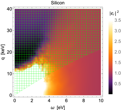
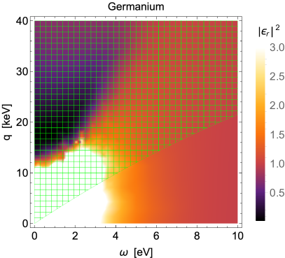
Figure 1: Modulus squared of the dielectric function, $|\varepsilon_{r}|^{2}$, as a function of the momentum transfer, $|\mathbf{q}|$, and of the deposited energy $\omega$ for Si (left panel) and Ge (right panel). For the generalised susceptibilities that receive in-medium corrections ($\chi_{n_{0}n_{0}}$, $\chi_{j_{Mm}j_{Ml}}$ and $\Delta\chi_{j_{Ml}n_{0}}$ in the case of non-spin-polarised materials), $|\varepsilon_{r}|^{2}$ determines the size and nature of such corrections. For example, $|\varepsilon_{r}|^{2}>1$ corresponds to a suppression of the material response to an external DM perturbation associated with screening, whereas $|\varepsilon_{r}|^{2}<1$ implies an amplification of the material response due to collective excitations. In both panels, we superimpose a green grid over the points that fulfil $v_{\rm min}>v_{\rm max}$, and which are thus not kinematically accessible for a DM particle mass of 10 MeV. Collective excitations correspond to energies and momenta in the black regions, and are thus kinematically inaccessible.

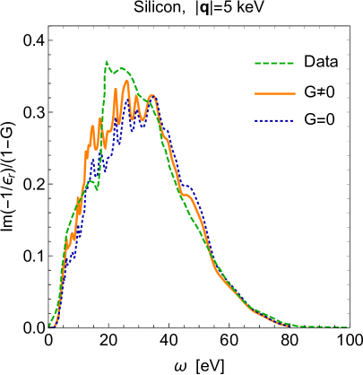
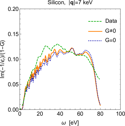
Figure 2: Silicon loss function, $\Im(-1/\varepsilon_{r})/(1-G)$, versus deposited energy $\omega$ for $|\mathbf{q}|=5$ keV (left panel) and $|\mathbf{q}|=7$ keV (right panel). In both panels, the dashed green lines represent experimental data from Weissker et al. (2010), while the dotted blue lines correspond to theoretical predictions based on Eq. (101) with $G=0$ and using the density-density response function $\chi_{n_{0}n_{0}}$ computed in Knapen et al. (2022) with the GPAW code Mortensen et al. (2005) in the RPA limit. With these settings, the dotted blue lines account for exchange and correlation in the calculation of $\chi_{n_{0}n_{0}}$, but not in the relation between $\chi_{n_{0}n_{0}}$ and $\varepsilon_{r}$. The solid orange lines correspond to our theoretical predictions based on Eq. (101) with $G\neq 0$. They thus account for exchange and correlation both in the calculation of $\chi_{n_{0}n_{0}}$ and in the relation between $\chi_{n_{0}n_{0}}$ and $\varepsilon_{r}$. While $G\neq 0$ implies a relatively small correction to $\Im(-1/\varepsilon^{\rm GPAW}_{r})$, it improves the agreement between theory and observations by increasing the loss function at small $\omega$, while decreasing the latter for intermediate values of $\omega$.

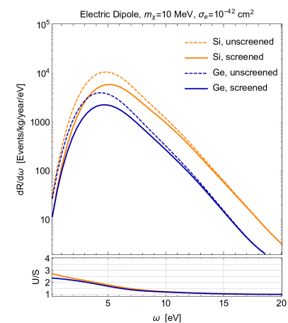
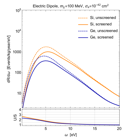
Figure 3: Differential rate of electronic transition per unit detector mass as a function of the deposited energy $\omega$ in Si (orange) or Ge (blue) crystals for a reference DM-electron scattering cross section of $10^{-42}$ cm². We assume that the DM particle is characterised by an electric dipole and has a mass of either 10 MeV (left panels) or 100 MeV (right panels). Solid lines correspond to screened interactions, i.e. $|\varepsilon_{r}|^{2}\neq 1$, whereas dashed lines neglect in-medium effects, i.e. $|\varepsilon_{r}|^{2}=1$. The bottom panels report the unscreened to screened rate ratio as function of $\omega$ for the germanium and silicon curves in the corresponding top panel.

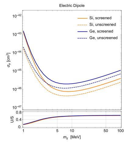
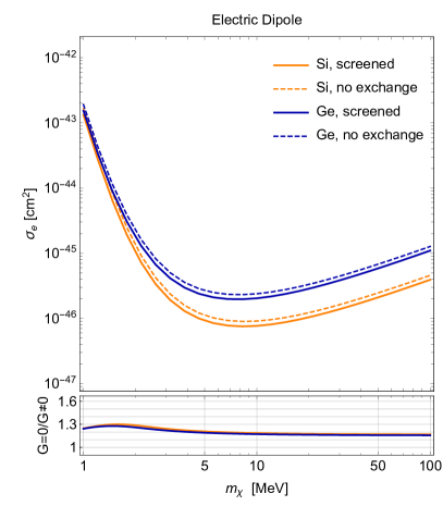
Figure 4: Projected 90% C.L. exclusion limits on the reference cross section $\sigma_{e}$ as a function of the DM particle mass $m_{\chi}$ for electric dipole DM. We assume a kg-year exposure in hypothetical background-free detectors made of either Si (orange lines) or Ge (blue lines) crystals. Solid lines correspond to predictions obtained accounting for in-medium as well as exchange and correlation effects ($G\neq 0$), whereas dashed lines neglect either the former (left panels) or the latter (right panels). The bottom panels report the ratios between dashed and solid lines of the same colour (i.e. same target) in the corresponding top panels.

VI Application to dark matter direct detection

An important result we have derived from Eq. (102) is that only the three generalised susceptibilities $\Im(\chi_{n_{0}n_{0}})$, $\Im(\chi_{j_{Ml}j_{Mm}})$ and $\Im(\Delta\chi_{j_{Ml}n_{0}})$ receive in-medium corrections for non-spin-polarised detector materials, i.e. materials where spin-up and spin-down electrons have the same wave functions for a given band index and reciprocal space vector. Focusing on DM models that generate these susceptibilities, we now apply the formalism developed in the previous sections to calculate the expected rates of DM-induced electronic transitions and the associated sensitivity of future experiments based on Ge and Si crystals.

VI.1 Electronic transition rates and exclusion limits

In this analysis, we focus on models where the DM particle is characterised by either an anapole or an electric dipole moment. This allows us to place the emphasis on the impact of in-medium effects, as well as of a non-zero local field factor $G$ on the calculated electron transition rates. In the case of DM candidates with an anapole moment, we are interested in external DM perturbations described by the potential in Eq. (42) with Catena et al. (2020),

$$c^{s}_{8} =8em_{e}m_{\chi}\frac{g}{\Lambda^{2}}$$

$$c^{s}_{9} =-8em_{e}m_{\chi}\frac{g}{\Lambda^{2}}\,,$$ (135)

and all other coupling constants set to zero. In the case of DM candidates with an electric dipole moment, we assume

$$c^{\ell}_{11}= \frac{16em_{\chi}m_{e}^{2}}{q_{\rm ref}^{2}}\frac{g}{\Lambda}\,,$$ (136)

with no other coupling constants different from zero. The dimensionless constant $g$ and the mass scale $\Lambda$ are in general different in Eqs. (135) and (136), although here we denote them with the same symbol for simplicity. By analogy with previous studies of anapole DM in the context of DM-nucleon scattering Del Nobile et al. (2013), we express $c^{s}_{8}$ and $c^{s}_{9}$ in terms of a reference DM-electron scattering cross section defined by

$$\sigma_{e}\equiv 2\alpha\,\frac{g^{2}\mu^{2}}{\Lambda^{4}}\,.$$ (137)

Similarly, in the case of electric dipole DM, e.g. Del Nobile et al. (2014), we introduce the reference DM-electron scattering cross section,

$$\sigma_{e}\equiv 4\alpha\,\frac{g^{2}}{\Lambda^{2}}\,.$$ (138)

In terms of generalised susceptibilities, the electric dipole DM model involves the density-density response function only, $\Im(\chi_{n_{0}n_{0}})$, whereas the anapole DM model is associated with the generalised susceptibilities $\Im(\chi_{n_{0}n_{0}})$, $\Im(\chi_{j_{Ml}j_{Mm}})$ and $\Im(\Delta\chi_{j_{Ml}n_{0}})$. As shown in Sec. V.2, for materials described by Eq. (126) in-medium corrections to $\Im(\chi_{n_{0}n_{0}})$, $\Im(\chi_{j_{Ml}j_{Mm}})$ and $\Im(\Delta\chi_{j_{Ml}n_{0}})$ depend on the ratio $\Im(\varepsilon_{r})/[|\varepsilon_{r}|^{2}(1-G)]$, known as the loss function. We have also seen that in-medium effects vanish in the $|\varepsilon_{r}|^{2}\rightarrow 1$ limit, which motivates a study of how $|\varepsilon_{r}|^{2}$ varies with $\mathbf{q}$ and $\omega$.

Fig. 1 shows $|\varepsilon_{r}|^{2}$ (not to be confused with $|\varepsilon^{\rm GPAW}_{r}|^{2}$), as a function of the momentum transfer, $|\mathbf{q}|$, and of the deposited energy $\omega$ for Si (left panel) and Ge (right panel) crystals. As anticipated in Sec. IV.3, $|\varepsilon_{r}|^{2}>1$ corresponds to a suppression of the generalised susceptibilities that receive in-medium corrections ($\chi_{n_{0}n_{0}}$, $\chi_{j_{Ml}j_{Mm}}$ and $\Delta\chi_{j_{Ml}n_{0}}$ in the case of non-spin-polarised materials) that is due to the screening of $n_{\rm ext}$ in Eq. (108). Similarly, $|\varepsilon_{r}|^{2}<1$ implies an amplification of the material response due to collective excitations. From Fig. 1 we thus expect collective excitations to be important in a region around $|\mathbf{q}|\sim$20 keV and $\omega\sim$1 eV. However, this region is not kinematically accessible in non-relativistic DM-electron scattering. To visualise this point, in both panels of Fig. 1, we superimpose a green grid over the points that fulfil the inequality $v_{\rm min}>v_{\rm max}$ for $m_{\chi}=10$ MeV, where $v_{\rm min}=\omega/q+q/(2m_{\chi})$ and $v_{\rm max}=v_{e}+v_{\mathrm{esc}}$. The same conclusion applies to different values of the DM particle mass.

Let us now focus on the Si loss function directly. Fig. 2 shows $\Im(\varepsilon_{r})/[|\varepsilon_{r}|^{2}(1-G)]$ as a function of the deposited energy $\omega$ for two representative values of the momentum transfer, namely $|\mathbf{q}|=5$ keV (left panel) and $|\mathbf{q}|=7$ keV (right panel). The dashed green lines in the two panels of Fig. 2 represent experimental data from Weissker et al. (2010), extracted from Fig. 1 of Knapen et al. (2022). In the same panels, the dotted blue lines correspond to theoretical predictions based on Eq. (101) with $G=0$ and the density-density response function $\chi_{n_{0}n_{0}}$ computed in Knapen et al. (2022) with the GPAW code Mortensen et al. (2005) in the RPA limit. Consequently, the dotted blue lines in the figure account for exchange in the calculation of $\chi_{n_{0}n_{0}}$, but not in the relation between $\chi_{n_{0}n_{0}}$ and $\varepsilon_{r}$. In contrast, the solid orange lines in the two panels of Fig. 2 correspond to our theoretical predictions based on Eq. (101) with $G\neq 0$. They thus account for exchange both in the calculation of $\chi_{n_{0}n_{0}}$ and in the relation between $\chi_{n_{0}n_{0}}$ and $\varepsilon_{r}$. While $G\neq 0$ implies a relatively small correction to the Si loss function, it improves the agreement between theory and experiment by increasing the loss function at small $\omega$, while decreasing it for larger $\omega$ values. We find a qualitatively similar behaviour for the Ge loss function (not shown).

Focusing on Ge and Si crystals, let us now calculate the differential rate of DM-induced electronic transitions per unit detector mass, ${\rm d}R/{\rm d}\omega$, within our generalised susceptibility formalism. Fig. 3 shows the differential rate ${\rm d}R/{\rm d}\omega$ as a function of $\omega$ for the case of electric dipole DM and a reference DM-electron scattering cross section of $10^{-42}$ cm². The left panels refer to a DM particle mass of 10 MeV, while the right panels correspond to $m_{\chi}=$ 100 MeV. While the top panels show the rate ${\rm d}R/{\rm d}\omega$ for a given DM-electron scattering cross section in different targets with and without in-medium effects, the bottom panels in the figure report the corresponding rate ratios to facilitate the comparison of distinct calculations. Specifically, the solid lines in the top panels account for in-medium effects in Si (orange) and Ge (blue) crystals, while the dashed lines assume $|\varepsilon_{r}|^{2}=1$. At the same time, the bottom panels in Fig. 3 report the unscreened to screened rate ratio as a function of $\omega$ for the crystals and mass in the corresponding top panel. As one can see from Fig. 3, in-medium corrections to $\Im(\chi_{n_{0}n_{0}})$ suppress the rate of DM-induced electronic transitions in crystals by a factor of 2 or 3 for $\omega$ below about $5$ eV, while they are negligible for $\omega$ larger than $15$ eV. The amplitude of the in-medium corrections for dipole DM is comparable with what was found in Knapen et al. (2022) focusing on models where DM couples to the density $n_{0}$ via the exchange of a heavy or light mediator, which, within our notation, would correspond to $\mathcal{M}=c^{s}_{1}\langle\mathcal{O}_{1}\rangle$ and $\mathcal{M}=c^{\ell}_{1}(q_{\rm ref}/q)^{2}\langle\mathcal{O}_{1}\rangle$, respectively.

Let us now focus on the impact of in-medium effects and electron exchange on the expected sensitivity of Ge and Si detectors. Fig. 4 shows the expected 90% confidence level (C.L.) exclusion limits on the reference cross section $\sigma_{e}$ as a function of the DM mass $m_{\chi}$ for electric dipole DM. We assume a kg-year exposure in hypothetical background-free detectors made of either Si (orange lines) or Ge (blue lines) crystals. The solid lines in the top panels correspond to predictions obtained accounting for in-medium as well as exchange effects ($G\neq 0$), whereas the dashed lines neglect either the former (left panel) or the latter (right panel). The bottom panels in Fig. 4 report the ratios between dashed and solid lines of the same colour in the corresponding top panels. From Fig. 4, we conclude that neglecting screening effects in the calculation of the expected 90% C.L. exclusion limits for electric dipole DM leads to an order one error on $\sigma_{e}$, whereas neglecting the exchange factor $G$ in the relation between the dielectric function $\varepsilon_{r}$ and $\chi_{n_{0}n_{0}}$ induces a $10\%$ error on $\sigma_{e}$.

In contrast, in-medium corrections are found to be negligible in the case of anapole DM, where the rate of electron transitions receives large contributions from the transverse components of $\Im(\chi_{j_{Ml}j_{Mm}})$, which are unscreened in nearly isotropic materials, and from $\Im\chi_{j_{5l}^{\dagger}j_{5m}}$, which is unscreened in non-spin-polarised detectors. For this reason, we do not report here the corresponding differential rate per unit detector mass and expected sensitivity studies.

Since the unscreened transverse components of $\Im(\chi_{j_{Ml}j_{Mm}})$ generically tend to “wash out” in-medium effects in electron transition rate calculations, and the generalised susceptibility $\Im(\Delta\chi_{j_{Ml}n_{0}})$ always appears together with $\Im(\chi_{j_{Ml}j_{Mm}})$, we arrive at the important conclusion that DM has to couple to the electron density $n_{0}$ alone for in-medium effects to be important in the DM-electron scattering in non-spin-polarised and nearly isotropic materials.

VI.2 Comparison with previous results

We now compare our expression for the rate of DM-induced electronic transitions in materials, Eq. (41), with the results found in Catena et al. (2021) for electronic transitions in semiconductor crystals assuming Bloch wave functions of the type

$$\psi_{i}(\mathbf{r}_{1}) =\phi_{i}(\mathbf{r}_{1})\,\eta^{\sigma}$$

$$\psi_{f}(\mathbf{r}_{1}) =\phi_{f}(\mathbf{r}_{1})\,\eta^{\sigma^{\prime}}\,,$$ (139)

for the initial and final state electrons, respectively. The $\eta^{\sigma}$ and $\eta^{\sigma^{\prime}}$ spinors are defined in the text above Eq. (67), whereas the $\phi_{i}(\mathbf{r}_{1})$ and $\phi_{f}(\mathbf{r}_{1})$ spatial wave functions are given in Eq. (113). When the electron spin wave function factorises as in Eq. (139) and as assumed in Catena et al. (2021), the matrix elements in Eq. (38) can be evaluated as in the following example,

$$|\langle f|e^{-i\mathbf{q}\cdot\mathbf{r}_{1}}\boldsymbol{\sigma}_{e}|i\rangle|^{2}= \sum_{\sigma\sigma^{\prime}}\eta^{\sigma^{\prime}\dagger}\boldsymbol{\sigma}_{e}\eta^{\sigma}\cdot\eta^{\sigma\dagger}\boldsymbol{\sigma}_{e}\eta^{\sigma^{\prime}}\langle f||e^{-i\mathbf{q}\cdot\mathbf{r}_{1}}||i\rangle|^{2}$$

$$= \mathrm{Tr}(\boldsymbol{\sigma}_{e}\cdot\boldsymbol{\sigma}_{e})\,\langle f||e^{-i\mathbf{q}\cdot\mathbf{r}_{1}}||i\rangle|^{2}$$ (140)

where

$$\langle f|\sigma_{e,l}e^{-i\mathbf{q}\cdot\mathbf{r}_{1}}|i\rangle\equiv\eta^{\sigma^{\prime}\dagger}\sigma_{e,l}\eta^{\sigma}\langle f||e^{-i\mathbf{q}\cdot\mathbf{r}_{1}}||i\rangle\,,$$ (141)

while $\sigma_{e,l}$ is the $l$-th Pauli matrix and $\boldsymbol{\sigma}_{e}$ a spatial vector. By inserting Eqs. (139) and (112) and the explicit expressions for the electron densities and currents, Eq. (32), into our differential rate formula, Eq. (40), we finally obtain

$${\rm d}\Gamma=\frac{{\rm d}\mathbf{q}}{(2\pi)^{3}} \int{\rm d}\omega\left(\frac{1}{8m_{e}^{2}m_{\chi}^{2}V}\right)\delta(\omega+\Delta E_{\chi})$$

$$\times\Big{[}A|f|^{2}+B_{(lm)}\,\Im(if_{l}^{*}f_{m})+B_{[lm]}\,\Re(if_{l}^{*}f_{m})$$

$$+C_{l}\,\Re(ff^{*}_{l})+\widetilde{C}_{l}\,\Im(ff^{*}_{l})\Big{]}\,,$$ (142)

where

$$A= ~{}\langle F^{*}_{0}F_{0}\rangle+\frac{q^{2}}{4m_{e}^{2}}\langle F^{*}_{A}F_{A}\rangle+\langle\mathbf{F}^{*}_{5}\cdot\mathbf{F}_{5}\rangle$$

$$+\frac{1}{4m_{e}^{2}}\left[\langle|\mathbf{q}\cdot\mathbf{F}_{M}|^{2}\rangle+\left(q^{2}\delta_{lm}-q_{l}q_{m}\right)\langle F^{*}_{El}F_{Em}\rangle\right]$$

$$+\frac{q_{l}}{m_{e}}\Re\langle F^{*}_{Ml}F_{0}\rangle+\frac{q_{l}}{m_{e}}\Re\langle F_{A}^{*}F_{5l}\rangle$$

$$+\frac{q_{i}}{m_{e}}\varepsilon_{ilm}\Im\langle F_{5l}^{*}F_{Em}\rangle\,,$$ (143)

while

$$B_{(lm)}= ~{}\langle F_{A}^{*}F_{A}\rangle\delta_{lm}+\Re\langle F_{Ml}^{*}F_{Mm}\rangle$$

$$+(\delta_{ij}\delta_{lm}-\delta_{im}\delta_{jl})\langle F_{Ei}^{*}F_{Ej}\rangle$$

$$B_{[lm]}= ~{}2\varepsilon_{ilm}\langle F_{Ei}^{*}F_{A}\rangle+\Im\langle F_{Ml}^{*}F_{Mm}\rangle\,,$$ (144)

and

$$C_{l}= ~{}\frac{q_{l}}{m_{e}}\langle F_{A}^{*}F_{A}\rangle+\frac{q_{m}}{m_{e}}\Re\langle F_{Ml}^{*}F_{Mm}\rangle$$

$$+\frac{q_{m}}{m_{e}}(\delta_{ij}\delta_{lm}-\delta_{im}\delta_{jl})\langle F_{Ei}^{*}F_{Ej}\rangle$$

$$+2\Re\langle F_{Ml}^{*}F_{0}\rangle+2\Re\langle F_{A}^{*}F_{5l}\rangle+2\varepsilon_{lij}\Im\langle F_{5i}^{*}F_{Ej}\rangle\,,$$

$$\widetilde{C}_{l}= ~{}-2\Im\langle F_{Ml}^{*}F_{0}\rangle-2\Im\langle F_{A}^{*}F_{5l}\rangle-2\varepsilon_{lij}\Re\langle F_{5i}^{*}F_{Ej}\rangle\,.$$ (145)

In all equations, a sum over repeated three-dimensional indices is understood. Obtaining Eq. (142), we use the identities

$$\mathrm{Tr}(\sigma_{e,i})=0$$

$$\mathrm{Tr}(\sigma_{e,i}\sigma_{e,j})=2\delta_{ij}\,.$$ (146)

Eq. (146) implies that many of the correlation functions that could in principle contribute to the differential rate ${\rm d}\Gamma$ are actually zero. In particular, all correlation functions linear in $\boldsymbol{\sigma}_{e}$ vanish. This is in general not true when spin up and spin down electrons have different wave functions, in contrast with Eq. (139), or many-body wave functions are used in the evaluation of the correlation functions $K_{j^{\dagger}_{\beta}j_{\alpha}}$.

By inserting the explicit expressions for the quadratic “strength functions” given in Appendix A into Eq. (145), we find that the total rate $\mathscr{R}$ resulting from Eqs. (41), (142) and (145) coincides with that given in Catena et al. (2021), with the exception of the coefficient in front of the $c_{14}c_{15}W_{5}$ term, which we find here to be $-1/8$, but which is erroneously reported to be $-1/2$ in Catena et al. (2021).

VII Summary and outlook

Within the non-relativistic effective theory of DM-electron interactions, we identified the densities and currents a spin-1/2 DM particle can couple to in a material, and found their corresponding electromagnetic analogues in a $1/c$ expansion of the Dirac Hamiltonian. Specifically, we found that DM can in general perturb a solid state system by coupling to the electron density, the paramagnetic current, the spin current, the scalar product of spin and paramagnetic current, as well as the Rashba spin-orbit current in the material. In the $(1/c)$ expansion of the Dirac Hamiltonian, the first, second and third couplings arise at order $(1/c)^{0}$, while the last two couplings originate at order $(1/c)^{2}$. We then wrote down the explicit expression for the time dependent effective potential that describes the scattering of DM particles by the electrons bound to a solid-state system, $V_{\rm eff}^{ss^{\prime}}(t)$ in Eq. (42), in terms of the five densities and currents listed above.

We interpreted the effective potential $V_{\rm eff}^{ss^{\prime}}(t)$ as an external perturbation in linear response theory, and identified the generalised susceptibilities that describe the response of a generic solid-state system to the perturbation $V_{\rm eff}^{ss^{\prime}}(t)$ by extending the Kubo formula to the case of DM-electron scattering in materials. We then combined the extended Kubo formula, Eq. (45), with Fermi’s golden rule to express the rate of DM-induced electronic transitions in a solid state system in terms of the generalised susceptibilities associated with the external perturbation $V_{\rm eff}^{ss^{\prime}}(t)$.

This expression for the electronic transition rate allowed us to factorise in a neat manner the material physics contribution, encoded in a set of generalised susceptibilities, from the particle physics input. Interestingly, this factorisation enables the use of existing experimental data on the generalised susceptibilities associated with $V_{\rm eff}^{ss^{\prime}}(t)$ to calibrate theoretical predictions for the rate of DM-induced electronic transitions in a given detector.

In order to evaluate our transition rate formula, i.e. Eq. (60), we applied the equation of motion method. This approach allowed us to express the set of generalised susceptibilities we identified in this work as the mean-field solution to a time-evolution equation, for which we also provided a useful diagrammatic interpretation. This solution, see Eq. (102), is one of the main results of our work.

An important conclusion we drew from Eq. (102) is that only three generalised susceptibilities receive corrections that are associated with screening or collective excitations in the case of non-spin-polarised materials, i.e. materials where spin up and spin down electrons have the same wave functions for a given band index and reciprocal space vector. These generalised susceptibilities are $\Im(\chi_{n_{0}^{\dagger}n_{0}})$, $\Im(\chi_{j^{\dagger}_{Ml}j_{Mm}})$ and $\Im(\Delta\chi_{j^{\dagger}_{Ml}n_{0}})$, where $n_{0}$ is the electron density and $j_{Ml}$, $l=1,2,3$ is the paramagnetic current. We also found that the in-medium corrections to $\Im(\chi_{n_{0}^{\dagger}n_{0}})$, $\Im(\Delta\chi_{j^{\dagger}_{Ml}n_{0}})$ and $\Im(\chi_{j^{\dagger}_{Ml}j_{Mm}})$ can be expressed in terms of the electron loss function in the case of isotropic materials. Another conclusion we drew from Eq. (102), is that it captures exchange effects that would be missed in the random phase approximation (RPA).

Finally, we applied the formalism developed in this work to calculate the expected electronic transition rate and sensitivity of hypothetical DM direct detection using Ge and Si crystals as detector materials. This calculation was performed by the combined use of the computer programmes QEdark-EFT Urdshals and Matas (2021), QEdark Essig et al. (2016) and DarkELF Knapen et al. (2022) as explained in Sec. VI.1. Emphasis was placed on quantifying the importance of in-medium corrections as well as exchange effects. For example, we found that neglecting screening effects in the calculation of the expected 90% C.L. exclusion limits for DM candidates with an electric dipole (modelled via the potential $V_{\rm eff}^{ss^{\prime}}(t)$) leads to an $\mathcal{O}(1)$ error in the reference DM-electron scattering cross section, $\sigma_{e}$, whereas neglecting electron exchange in the relation between dielectric function, $\varepsilon_{r}$, and density-density response function, $\chi_{n_{0}^{\dagger}n_{0}}$, induces a $10\%$ error in $\sigma_{e}$.

In contrast, in-medium corrections were found to be negligible in the case of anapole DM, because the rate of electron transitions in detector materials receives in this case large contributions from the transverse components of the current-current response functions $\Im(\chi_{j_{Ml}^{\dagger}j_{Mm}})$ and from $\Im\chi_{j_{5l}^{\dagger}j_{5m}}$. The former is unscreened in nearly isotropic materials, while the latter is unscreened in non-spin-polarised detectors.

More generally, we arrived at the important conclusion that, if screening of the transverse responses is neglected, then in-medium effects are significant in the DM scattering from non-spin-polarized materials only when the DM couples to the electron density $n_{0}$ alone.  This is due to the fact that the unscreened transverse components of $\Im(\chi_{j_{Ml}^{\dagger}j_{Mm}})$ generically tend to “wash out” in-medium effects in electron transition-rate calculations, and that $\Im(\Delta\chi_{j_{Ml}^{\dagger}n_{0}})$ always appears together with $\Im(\chi_{j_{Ml}^{\dagger}j_{Mm}})$.

Summarising, the linear response theory for light DM direct detection we developed in this work paves the way for the study of in-medium effects in the presence of general DM-electron interactions. It provides a framework for using existing or future experimental measurements of the generalised susceptibilities $\chi_{j_{\alpha}j_{\beta}}$ to calibrate theoretical predictions of the rate of DM-induced electronic transitions in detector materials. Finally, it can be straightforwardly extended to the case of spin-polarised detectors, as well as to highly inhomogeneous or anisotropic materials. We leave these investigations for future work.

Appendix A Quadratic strength functions

In this appendix, we list explicit expressions for the functions $F_{0}^{ss^{\prime}}$, $F_{A}^{ss^{\prime}}$, $\mathbf{F}_{5}^{ss^{\prime}}$, $\mathbf{F}_{M}^{ss^{\prime}}$, and $\mathbf{F}_{E}^{ss^{\prime}}$. They are given by

$$F_{0}^{ss^{\prime}}= ~{}\xi^{s^{\prime}\dagger}\left[c_{1}+i\left(\frac{\mathbf{q}}{m_{e}}\times\mathbf{v}_{\chi}^{\perp}\right)\cdot\mathbf{S}_{\chi}c_{5}+\mathbf{v}_{\chi}^{\perp}\cdot\mathbf{S}_{\chi}\right.c_{8}$$

$$+\left.i\frac{\mathbf{q}}{m_{e}}\cdot\mathbf{S}_{\chi}c_{11}\right]\xi^{s}$$

$$F_{A}^{ss^{\prime}}= ~{}-\frac{1}{2}\xi^{s^{\prime}\dagger}\left[c_{7}+i\frac{\mathbf{q}}{m_{e}}\cdot\mathbf{S}_{\chi}~{}c_{14}\right]\xi^{s}$$

$$\mathbf{F}_{5}^{ss^{\prime}}= ~{}\frac{1}{2}\xi^{s^{\prime}\dagger}\left[i\frac{\mathbf{q}}{m_{e}}\times\mathbf{v}_{\chi}^{\perp}~{}c_{3}+\mathbf{S}_{\chi}c_{4}+\frac{\mathbf{q}}{m_{e}}~{}\frac{\mathbf{q}}{m_{e}}\cdot\mathbf{S}_{\chi}c_{6}\right.$$

$$+\left.\mathbf{v}_{\chi}^{\perp}c_{7}+i\frac{\mathbf{q}}{m_{e}}\times\mathbf{S}_{\chi}c_{9}+i\frac{\mathbf{q}}{m_{e}}c_{10}+\mathbf{v}_{\chi}^{\perp}\times\mathbf{S}_{\chi}c_{12}\right.$$

$$+\left.i\mathbf{v}_{\chi}^{\perp}\frac{\mathbf{q}}{m_{e}}\cdot\mathbf{S}_{\chi}~{}c_{14}+\frac{\mathbf{q}}{m_{e}}\times\mathbf{v}_{\chi}^{\perp}~{}\frac{\mathbf{q}}{m_{e}}\cdot\mathbf{S}_{\chi}~{}c_{15}\right]\xi^{s}$$

$$\mathbf{F}_{M}^{ss^{\prime}}= ~{}\xi^{s^{\prime}\dagger}\left[i\frac{\mathbf{q}}{m_{e}}\times\mathbf{S}_{\chi}c_{5}-\mathbf{S}_{\chi}c_{8}\right]\xi^{s}$$

$$\mathbf{F}_{E}^{ss^{\prime}}= ~{}\frac{1}{2}\xi^{s^{\prime}\dagger}\left[\frac{\mathbf{q}}{m_{e}}~{}c_{3}+i\mathbf{S}_{\chi}c_{12}-i{\mathbf{q}\over m_{e}}\frac{\mathbf{q}}{m_{e}}\cdot\mathbf{S}_{\chi}c_{15}\right]\xi^{s}\,,$$ (147)

where

$$\mathbf{v}_{\chi}^{\perp}=\left(\frac{\mathbf{p}+\mathbf{p}^{\prime}}{2m_{\chi}}\right)=\mathbf{v}-\frac{\mathbf{q}}{2m_{\chi}}\,,$$ (148)

$\mathbf{v}=\mathbf{p}/m_{\chi}$, $\mathbf{q}=\mathbf{p}-\mathbf{p}^{\prime}$ is the momentum transferred to the electron, and, finally, we shortened the notation by defining,

$$c_{i}\equiv\left(c_{i}^{s}+c^{\ell}_{i}\frac{q_{\rm ref}^{2}}{|\mathbf{q}|^{2}}\right)\,.$$ (149)

Furthermore, we list the quadratic strength functions used in Sec. III to calculate the rate of DM-induced electronic transitions in materials. They can be written as follows:

$$\langle F_{0}^{*}F_{0}\rangle =c_{1}^{2}+\frac{1}{4}\left|\frac{\mathbf{q}}{m_{e}}\times\mathbf{v}_{\chi}^{\perp}\right|^{2}c_{5}^{2}+\frac{v_{\chi}^{\perp 2}}{4}c_{8}^{2}+\frac{q^{2}}{4m_{e}^{2}}c_{11}^{2}\,,$$ (150)

$$\langle F_{A}^{*}F_{A}\rangle =\frac{1}{4}\left(c_{7}^{2}+\frac{q^{2}}{4m_{e}^{2}}c_{14}^{2}\right)\,,$$ (151)

$$\langle\mathbf{F}_{5}^{*}\cdot\mathbf{F}_{5}\rangle =\frac{1}{4}\bigg{(}\left|\frac{\mathbf{q}}{m_{e}}\times\mathbf{v}_{\chi}^{\perp}\right|^{2}c_{3}^{2}+\frac{3}{4}c_{4}^{2}+\frac{q^{4}}{4m_{e}^{4}}c_{6}^{2}$$

$$+v_{\chi}^{\perp 2}c_{7}^{2}+\frac{q^{2}}{2m_{e}^{2}}c_{9}^{2}+\frac{q^{2}}{m_{e}^{2}}c_{10}^{2}+\frac{v_{\chi}^{\perp 2}}{2}c_{12}^{2}$$

$$+\frac{q^{2}}{4m_{e}^{2}}v_{\chi}^{\perp 2}c_{14}^{2}+\left|\frac{\mathbf{q}}{m_{e}}\times\mathbf{v}_{\chi}^{\perp}\right|^{2}\frac{q^{2}}{4m^{2}_{e}}c_{15}^{2}$$

$$+\frac{q^{2}}{2m_{e}^{2}}c_{4}c_{6}+\left|\frac{\mathbf{q}}{m_{e}}\times\mathbf{v}_{\chi}^{\perp}\right|^{2}c_{14}^{2}c_{15}^{2}\bigg{)}\,,$$ (152)

$$\langle F^{*}_{Ml}F_{Mm}\rangle =\frac{1}{4m_{e}^{2}}\left(q^{2}\delta_{lm}-q_{l}q_{m}\right)c_{5}^{2}+\frac{1}{4}c_{8}^{2}\delta_{lm}$$

$$-\frac{i}{2}\varepsilon_{lmi}\frac{q_{i}}{m_{e}}c_{5}c_{8}\,,$$ (153)

$$\langle F^{*}_{El}F_{Em}\rangle =\frac{1}{4}\bigg{(}\frac{q_{l}q_{m}}{m_{e}^{2}}c_{3}^{2}+\frac{1}{4}\delta_{lm}c_{12}^{2}+\frac{q^{2}}{4m_{e}^{2}}\frac{q_{l}q_{m}}{m_{e}^{2}}c_{15}^{2}$$

$$-\frac{q_{l}q_{m}}{2m_{e}^{2}}c_{12}c_{15}\bigg{)}\,.$$ (154)

In addition, we made use of the following off-diagonal terms:

$$\langle F_{El}^{*}F_{A}\rangle =\frac{1}{4}\left(-\frac{q_{l}}{m_{e}}c_{3}c_{7}-\frac{q_{l}}{4m_{e}}c_{12}c_{14}+\frac{q_{l}}{4m_{e}}\frac{q^{2}}{m_{e}^{2}}c_{14}c_{15}\right)$$ (155)

$$\langle F_{Ml}^{*}F_{0}\rangle =-\frac{1}{4}(v_{\chi}^{\perp})_{l}c_{8}^{2}-\frac{i}{2}\left|\frac{\mathbf{q}}{m_{e}}\times\mathbf{v}_{\chi}^{\perp}\right|_{l}c_{5}c_{8}-\frac{i}{4}\frac{q_{l}}{m_{e}}c_{8}c_{11}$$ (156)

$$\langle F_{A}^{*}F_{5l}\rangle =-\frac{1}{4}(v_{\chi}^{\perp})_{l}c_{7}^{2}-\frac{q^{2}}{16m_{e}^{2}}(v_{\chi}^{\perp})_{l}c_{14}^{2}$$

$$-\frac{i}{4}\left(\frac{\mathbf{q}}{m_{e}}\times\mathbf{v}_{\chi}^{\perp}\right)_{l}c_{3}c_{7}-\frac{i}{4}\frac{q_{l}}{m_{e}}c_{7}c_{10}$$

$$+\frac{i}{16}\frac{q_{l}}{m_{e}}c_{4}c_{14}+\frac{i}{16}\frac{q^{2}}{m_{e}^{2}}\frac{q_{l}}{m_{e}}c_{6}c_{14}$$

$$+\frac{i}{16}\frac{q^{2}}{m_{e}^{2}}\left(\frac{\mathbf{q}}{m_{e}}\times\mathbf{v}_{\chi}^{\perp}\right)_{l}c_{14}c_{15}\,,$$ (157)

and, finally,

$$\varepsilon_{ilm}\langle F_{5l}^{*}F_{Em}\rangle =\frac{1}{4}\bigg{[}\frac{i}{m_{e}^{2}}\left(q_{i}q_{m}-q^{2}\delta_{mi}\right)(v_{\chi}^{\perp})_{m}c_{3}^{2}$$

$$-\frac{i}{2}(v_{\chi}^{\perp})_{i}c_{12}^{2}$$

$$+\frac{i}{4m_{e}^{2}}\left(\mathbf{q}\cdot\mathbf{v}_{\chi}^{\perp}q_{i}-q^{2}(v_{\chi}^{\perp})_{i}\right)\frac{q^{2}}{m_{e}^{2}}c_{15}^{2}$$

$$+\varepsilon_{ilm}(v_{\chi}^{\perp})_{l}\frac{q_{m}}{m_{e}}c_{3}c_{7}-\frac{q_{i}}{2m_{e}}c_{9}c_{12}$$

$$-\frac{5i}{4m_{e}^{2}}\left(\mathbf{q}\cdot\mathbf{v}_{\chi}^{\perp}q_{i}-q^{2}(v_{\chi}^{\perp})_{i}\right)c_{12}c_{15}$$

$$+\varepsilon_{ilm}(v_{\chi}^{\perp})_{l}\frac{q_{m}}{m_{e}}c_{12}c_{14}$$

$$-\frac{q^{2}}{4m_{e}^{2}}\varepsilon_{ilm}(v_{\chi}^{\perp})_{l}\frac{q_{m}}{m_{e}}c_{14}c_{15}\bigg{]}\,.$$ (158)

Appendix B Kubo formula for dark matter-electron scattering

We are interested in DM-induced perturbations to detector materials that can be described by the effective potential

$$V_{\rm eff}^{ss^{\prime}}(t)\equiv-\int{\rm d}\mathbf{r}\,B(\mathbf{r})S^{ss^{\prime}}(\mathbf{r},t)$$ (159)

where $B(\mathbf{r})$ is an operator acting on the wave functions of the electrons in the material and $S^{ss^{\prime}}(\mathbf{r},t)$ is the strength of the perturbation. $S^{ss^{\prime}}(\mathbf{r},t)$ depends on the initial and final DM particle spin configurations, $s$ and $s^{\prime}$. Each term in the effective potential actually used in this work, Eq. (30), has the form assumed here in Eq. (159) for illustrative purposes. Under such perturbations, the density matrix $\rho$ of the given detector material evolves according to

$$\frac{{\rm d}\rho(t)}{{\rm d}t}=i\left[\rho(t),H_{0}+V^{ss^{\prime}}_{\rm eff}(t)\right]$$ (160)

where $H_{0}$ is the Hamiltonian of the system in the absence of external perturbations. By imposing $\rho(t\rightarrow-\infty)=\rho_{0}$, where $\rho_{0}$ is the density matrix when $V^{ss^{\prime}}_{\rm eff}=0$, and using

$$\frac{{\rm d}}{{\rm d}t}\Big{[}e^{iH_{0}t}\rho(t)\,e^{-iH_{0}t}\Big{]}=ie^{iH_{0}t}\left[\rho(t),V^{ss^{\prime}}_{\rm eff}(t)\right]e^{-iH_{0}t}\,,$$ (161)

Eq. (160) can conveniently be rewritten in an integral form,

$$\rho(t)=\rho_{0}+i\int_{-\infty}^{t}{\rm d}t^{\prime}e^{-iH_{0}(t-t^{\prime})}\left[\rho(t^{\prime}),V^{ss^{\prime}}_{\rm eff}(t^{\prime})\right]e^{iH_{0}(t-t^{\prime})}\,.$$ (162)

At first order in $V^{ss^{\prime}}_{\rm eff}$, Eq. (162) admits the following solution

$$\rho(t)=\rho_{0}+i\int_{-\infty}^{t}{\rm d}t^{\prime}e^{-iH_{0}(t-t^{\prime})}\left[\rho_{0},V^{ss^{\prime}}_{\rm eff}(t^{\prime})\right]e^{iH_{0}(t-t^{\prime})}\,.$$ (163)

We can now use Eq. (163) to calculate the expectation value of any observable $A(\mathbf{r},t=0)\equiv A(\mathbf{r})$. This is given by

$$\langle A\rangle =\mathrm{Tr}\left\{A\rho\right\}$$

$$=\mathrm{Tr}\left\{A\rho_{0}\right\}+\langle\Delta A\rangle$$ (164)

where $\langle\Delta A\rangle$ is the induced perturbation in the observable $A$, namely

$$\langle\Delta A(\mathbf{r},t)\rangle= i\mathrm{Tr}\left\{\int_{-\infty}^{t}{\rm d}t^{\prime}\,A(\mathbf{r},t-t^{\prime})\left[\rho_{0},V^{ss^{\prime}}_{\rm eff}(t^{\prime})\right]\right\}$$

$$= -i\int_{-\infty}^{t}{\rm d}t^{\prime}\,\mathrm{Tr}\left\{\rho_{0}\left[A(\mathbf{r},t-t^{\prime}),V^{ss^{\prime}}_{\rm eff}(t^{\prime})\right]\right\}$$

$$= i\int_{-\infty}^{t}{\rm d}t^{\prime}\int{\rm d}\mathbf{r}^{\prime}\,\Big{\langle}\left[A(\mathbf{r},t-t^{\prime}),B(\mathbf{r}^{\prime})\right]\Big{\rangle}$$

$$\times S^{ss^{\prime}}(\mathbf{r}^{\prime},t^{\prime})$$

$$= i\int_{-\infty}^{t}{\rm d}t^{\prime}\int{\rm d}\mathbf{r}^{\prime}\,\Big{\langle}\left[A(\mathbf{r},t),B(\mathbf{r}^{\prime},t^{\prime})\right]\Big{\rangle}$$

$$\times S^{ss^{\prime}}(\mathbf{r}^{\prime},t^{\prime})\,,$$ (165)

where $A(\mathbf{r},t)=\exp(iH_{0}t)A(\mathbf{r})\exp(-iH_{0}t)$, and similarly for $B(\mathbf{r}^{\prime},t^{\prime})$. Introducing now the generalised susceptibility

$$\chi_{AB}(\mathbf{r}-\mathbf{r}^{\prime},t-t^{\prime})=i\theta(t-t^{\prime})\Big{\langle}\left[A(\mathbf{r},t),B(\mathbf{r}^{\prime},t^{\prime})\right]\Big{\rangle}$$ (166)

we obtain the Kubo formula for DM-electron scattering, namely

$$\langle\Delta A(\mathbf{r},t)\rangle=\int_{-\infty}^{t}{\rm d}t^{\prime}\int{\rm d}\mathbf{r}^{\prime}\,\chi_{AB}(\mathbf{r}-\mathbf{r}^{\prime},t-t^{\prime})S^{ss^{\prime}}(\mathbf{r}^{\prime},t^{\prime})$$ (167)

which describes the response to the DM-induced perturbation $V^{ss^{\prime}}_{\rm eff}$ of a given observable $A$ in a detector material.

Appendix C Spectral representation of generalised susceptibilities

In this appendix, we derive the spectral representations for the correlation function $K_{j_{\alpha}j_{\beta}}$ and the generalised susceptibility $\chi_{j_{\alpha}j_{\beta}}$ that we use in Sec. III. We treat the case of translationally invariant systems, in which both $K_{j_{\alpha}j_{\beta}}$ and $\chi_{j_{\alpha}j_{\beta}}$ depend on the relative distance $(\mathbf{r}-\mathbf{r}^{\prime})$ between the spatial points at which the densities or current densities $j_{\alpha}$ and $j_{\beta}$ are evaluated, and not on $\mathbf{r}$ and $\mathbf{r}^{\prime}$ separately. Consequently, the Fourier transform with respect to $(\mathbf{r}-\mathbf{r}^{\prime})$ of the correlation function $K_{j_{\alpha}j_{\beta}}(\mathbf{r}-\mathbf{r}^{\prime},t-t^{\prime})$ can be written as follows

$$K_{j_{\alpha}j_{\beta}}(\mathbf{q},t-t^{\prime}) =\int{\rm d}(\mathbf{r}-\mathbf{r}^{\prime})e^{-i\mathbf{q}\cdot(\mathbf{r}-\mathbf{r}^{\prime})}\langle j_{\alpha}(\mathbf{r},t)j_{\beta}(\mathbf{r}^{\prime},t^{\prime})\rangle$$

$$=\frac{1}{V}\langle j_{\alpha}(\mathbf{q},t)j_{\beta}(-\mathbf{q},t^{\prime})\rangle\,.$$ (168)

Furthermore, the Fourier transform of $K_{j_{\alpha}j_{\beta}}(\mathbf{q},t-t^{\prime})$ with respect to $t-t^{\prime}$ can be expressed in terms of a complete set of energy eigenstates, denoted here by $|\psi_{n}\rangle$. One finds,

$$K_{j_{\alpha}j_{\beta}}(\mathbf{q},\omega)= \int_{-\infty}^{+\infty}{\rm d}(t-t^{\prime})e^{i\omega(t-t^{\prime})}K_{j_{\alpha}j_{\beta}}(\mathbf{q},t-t^{\prime})$$

$$= \frac{1}{V}\int_{-\infty}^{+\infty}{\rm d}(t-t^{\prime})e^{i\omega(t-t^{\prime})}\sum_{n,m}\frac{e^{-\overline{\beta}E_{n}}}{Z}$$

$$\times\langle\psi_{n}|j_{\alpha}(\mathbf{q},t)|\psi_{m}\rangle\langle\psi_{m}|j_{\beta}(-\mathbf{q},t^{\prime})|\psi_{n}\rangle$$ (169)

Translating now the operators $j_{\alpha}$ and $j_{\beta}$ to time $t=0$, we find

$$K_{j_{\alpha}j_{\beta}}(\mathbf{q},\omega)= \frac{1}{V}\sum_{n,m}\int_{-\infty}^{+\infty}{\rm d}(t-t^{\prime})e^{i\omega(t-t^{\prime})}$$

$$\times\frac{e^{-\overline{\beta}E_{n}}}{Z}e^{i(E_{n}-E_{m})(t-t^{\prime})}$$

$$\times\langle\psi_{n}|j_{\alpha}(\mathbf{q})|\psi_{m}\rangle\langle\psi_{m}|j_{\beta}(-\mathbf{q})|\psi_{n}\rangle\,,$$ (170)

with $j_{\alpha}(\mathbf{q})=j_{\alpha}(t=0,\mathbf{q})$ and $j_{\beta}(\mathbf{q})=j_{\beta}(t^{\prime}=0,\mathbf{q})$. Performing the integral over $(t-t^{\prime})$ explicitly, we finally obtain

$$K_{j_{\alpha}j_{\beta}}(\mathbf{q},\omega)= \frac{2\pi}{V}\sum_{n,m}\frac{e^{-\overline{\beta}E_{n}}}{Z}\delta(E_{n}-E_{m}+\omega)$$

$$\times\langle\psi_{n}|j_{\alpha}(\mathbf{q})|\psi_{m}\rangle\langle\psi_{m}|j_{\beta}(-\mathbf{q})|\psi_{n}\rangle$$ (171)

which is the spectral representation for the correlation function $K_{j_{\alpha}j_{\beta}}$ used in Sec. III. Similarly, the double Fourier transform of the generalised susceptibility $\chi_{j_{\alpha}j_{\beta}}$, namely

$$\chi_{j_{\alpha}j_{\beta}}(\mathbf{q},\omega)= \int_{-\infty}^{+\infty}{\rm d}(t-t^{\prime})e^{i\omega(t-t^{\prime})}\chi_{j_{\alpha}j_{\beta}}(\mathbf{q},t-t^{\prime})$$ (172)

can be written as

$$\chi_{j_{\alpha}j_{\beta}}(\mathbf{q},\omega)= \frac{i}{V}\int_{-\infty}^{+\infty}{\rm d}(t-t^{\prime})\theta(t-t^{\prime})e^{i\omega(t-t^{\prime})}$$

$$\times\sum_{n,m}\frac{e^{-\overline{\beta}E_{n}}}{Z}e^{i(E_{n}-E_{m})(t-t^{\prime})}$$

$$\times\langle\psi_{n}|j_{\alpha}(\mathbf{q})|\psi_{m}\rangle\langle\psi_{m}|j_{\beta}(-\mathbf{q})|\psi_{n}\rangle$$

$$\times\left(1-e^{-\overline{\beta}(E_{m}-E_{n})}\right)\,.$$ (173)

Using now the integral representation for the step function,

$$\theta(t-t^{\prime})=-\frac{1}{2\pi i}\int^{+\infty}_{-\infty}{\rm d}\omega\,\frac{e^{-i\omega(t-t^{\prime})}}{\omega+i\delta}\,,$$ (174)

we find

$$\chi_{j_{\alpha}j_{\beta}}(\mathbf{q},\omega)= -\frac{1}{V}\sum_{n,m}\frac{e^{-\overline{\beta}E_{n}}}{Z}$$

$$\times\langle\psi_{n}|j_{\alpha}(\mathbf{q})|\psi_{m}\rangle\langle\psi_{m}|j_{\beta}(-\mathbf{q})|\psi_{n}\rangle$$

$$\times\frac{\left(1-e^{-\overline{\beta}(E_{m}-E_{n})}\right)}{\omega+E_{n}-E_{m}+i\delta}\,,$$ (175)

which is the spectral representation for $\chi_{j_{\alpha}j_{\beta}}$ we use in Sec. III. The spectral representation for $\chi^{A}_{j_{\alpha}j_{\beta}}$ can be derived using

$$\theta(t^{\prime}-t)=\frac{1}{2\pi i}\int^{+\infty}_{-\infty}{\rm d}\omega\,\frac{e^{i\omega(t^{\prime}-t)}}{\omega-i\delta}\,.$$ (176)

One finds

$$\chi^{A}_{j_{\alpha}j_{\beta}}(\mathbf{q},\omega)= -\frac{1}{V}\sum_{n,m}\frac{e^{-\overline{\beta}E_{n}}}{Z}$$

$$\times\langle\psi_{n}|j_{\alpha}(\mathbf{q})|\psi_{m}\rangle\langle\psi_{m}|j_{\beta}(-\mathbf{q})|\psi_{n}\rangle$$

$$\times\frac{\left(1-e^{-\overline{\beta}(E_{m}-E_{n})}\right)}{\omega+E_{n}-E_{m}-i\delta}\,.$$ (177)

Before concluding, we notice that

$$\chi^{*}_{j^{\dagger}_{\beta}j^{\dagger}_{\alpha}}(\mathbf{q},\omega)= -\frac{1}{V}\sum_{n,m}\frac{e^{-\overline{\beta}E_{n}}}{Z}$$

$$\times\langle\psi_{n}|j^{\dagger}_{\beta}(\mathbf{q})|\psi_{m}\rangle^{*}\langle\psi_{m}|j^{\dagger}_{\alpha}(-\mathbf{q})|\psi_{n}\rangle^{*}$$

$$\times\frac{\left(1-e^{-\overline{\beta}(E_{m}-E_{n})}\right)}{\omega+E_{n}-E_{m}-i\delta}\,.$$ (178)

Since $\langle\psi_{n}|j^{\dagger}_{\beta}(\mathbf{q})|\psi_{m}\rangle^{*}=\langle\psi_{m}|j_{\beta}(-\mathbf{q})|\psi_{n}\rangle$, we finally obtain

$$\chi^{*}_{j^{\dagger}_{\beta}j^{\dagger}_{\alpha}}(\mathbf{q},\omega)=\chi^{A}_{j_{\alpha}j_{\beta}}(\mathbf{q},\omega)\,.$$ (179)