Distributed Quasi-Newton Method for Multi-Agent Optimization

Abstract

We present a distributed quasi-Newton (DQN) method, which enables a group of agents to compute an optimal solution of a separable multi-agent optimization problem locally using an approximation of the curvature of the aggregate objective function. Each agent computes a descent direction from its local estimate of the aggregate Hessian, obtained from quasi-Newton approximation schemes using the gradient of its local objective function. Moreover, we introduce a distributed quasi-Newton method for equality-constrained optimization (EC-DQN), where each agent takes Karush-Kuhn-Tucker-like update steps to compute an optimal solution. In our algorithms, each agent communicates with its one-hop neighbors over a peer-to-peer communication network to compute a common solution. We prove convergence of our algorithms to a stationary point of the optimization problem. In addition, we demonstrate the competitive empirical convergence of our algorithm in both well-conditioned and ill-conditioned optimization problems, in terms of the computation time and communication cost incurred by each agent for convergence, compared to existing distributed first-order and second-order methods. Particularly, in ill-conditioned problems, our algorithms achieve a faster computation time for convergence, while requiring a lower communication cost, across a range of communication networks with different degrees of connectedness, by leveraging information on the curvature of the problem.

I Introduction

The paradigm of optimization has been widely employed in model design and analysis [1, 2, 3, 4, 5], planning [6, 7, 8], and control [9, 10, 11], across broad problem domains. In many situations, the pertinent problem requires optimization over spatially-distributed data and agent-specific objective and constraints across a group of agents—referred to as the multi-agent problem. Privacy constraints and resource limitations often make aggregation of the problem data for centralized optimization intractable, thus rendering distributed optimization as a viable alternative for optimization. Via distributed optimization, each agent communicates with its local neighbors over a communication network to compute a common, optimal solution of the problem, without any access to the aggregate problem data over all agents. In this work, we not only consider unconstrained multi-agent problems, we also consider equality-constrained problems, noting that many existing distributed optimization algorithms (e.g., the broad class of distributed first-order methods) typically consider only unconstrained multi-agent optimization problems. Meanwhile, constrained multi-agent optimization problems arise in many settings, e.g., basis pursuit problems in signal processing.

Distributed first-order methods, such as distributed gradient descent methods, enable each agent to solve the aggregate multi-agent optimization problem by utilizing only the local gradient of its objective function [12, 13, 14]. However, distributed first-order methods generally exhibit slow convergence, particularly in ill-conditioned problems. In contrast, second-order methods—which utilize information on the higher-order derivatives of the problem, specifically the Hessian—provide faster convergence rates in these problems. By leveraging information on the curvature of the objective function, second-order methods provide a more effective descent direction for the minimization problem. However, computation of the Hessian often proves challenging, and sometimes intractable, in many problems. Quasi-Newton methods seek to address this challenge, by approximating the Hessian of the objective function, often at the expense of a decrease in the convergence rate. Further, we note that many existing distributed second-order and quasi-Newton methods either require significant computation and communication overhead to achieve fast convergence rates, from exact computation of the local Hessians, or suffer from slow convergence, when approximating the local Hessians [15, 16].

To address these challenges, we present a distributed quasi-Newton (DQN) method for unconstrained optimization, as well as its extension to equality-constrained optimization problems EC-DQN. These algorithms enable a group of agents to cooperatively compute an optimal solution locally, by leveraging the approximate curvature of the objective function. Each agent uses only its local gradients to estimate the Hessian of the aggregate objective function, while communicating with its local neighbors over a communication network. We prove convergence of our algorithms to a stationary solution of the aggregate optimization problem, provided the objective function is convex and smooth.

We examine the performance of DQN and EC-DQN in unconstrained and equality-constrained optimization problems, respectively, in comparison to existing distributed optimization algorithms. In well-conditioned problems, DQN performs competitively, in terms of the computation time required for convergence and the associated communication cost, in comparison to distributed first-order methods, especially in more-densely-connected communication networks, while performing better than distributed second-order methods. In addition, we demonstrate faster empirical convergence of DQN compared to other distributed first-order and second-order methods in ill-conditioned problems, where the distributed first-order methods achieve a low success rate in converging to the optimal solution on many problem instances. In ill-conditioned problems, DQN provides about a seven-times reduction in the communication cost of each agent compared to the best-competing second-order method, while achieving the fastest computation time across a range of communication networks. In the unconstrained logistic regression problem, DQN achieves the least communication cost, providing about an order of magnitude reduction in the communication cost compared to the best-competing second-order method, which is the only other method that converged on all problem instances. In the equality-constrained setting, EC-DQN achieves faster convergence in constrained basis pursuit denoising and logistic regression problems across communication networks with different degrees of connectedness. In particular, EC-DQN requires shorter computation times for convergence, with lower associated communication costs, especially in networks having a connectivity ratio of at least $0.57$.

We summarize our contributions as follows:

1. We derive a distributed quasi-Newton (DQN) method for unconstrained multi-agent optimization, enabling each agent to leverage information on the curvature of the objective function to improve convergence, especially in ill-conditioned problem settings.

2. Further, we present a distributed quasi-Newton method for equality-constrained optimization problems EC-DQN, which enables agents to utilize local first-order information to compute an optimal solution satisfying the problem constraints, without any associated projection procedure.

3. We demonstrate the superior performance of our algorithms DQN and EC-DQN in a variety of problems across a range of communication networks, particularly in ill-conditioned problems.

II Related Work

Distributed optimization methods have been widely developed for finite-sum unconstrained optimization problems [17, 18]. These algorithms can be broadly grouped into the following categories: distributed first-order methods, distributed primal-dual methods, and distributed second-order methods and closely-related quasi-Newton methods. In this section, we review notable algorithms within each of the enumerated categories, identifying the key distinguishing techniques employed by these algorithms.

The simplest distributed optimization algorithms extend the well-known centralized gradient descent algorithm to the distributed setting [19, 12]. In decentralized gradient descent algorithms, each agent updates its local copy of the problem variable in the direction of its local gradient, in contrast to the centralized case, where the problem variable is updated in the direction of the aggregate gradient. Noting that the local gradients of all agents are not necessarily collinear, these algorithms employ consensus techniques such as the linear consensus protocol, enabling all agents to agree on a common solution. Alternatively, some variants of decentralized gradient descent utilize the push-sum protocol to achieve consensus among the agents [20]. In generally, this subcategory of distributed first-order methods do not converge to an optimal solution of the aggregate optimization problem under a fixed step-size scheme, converging rather to a neighborhood of the optimal solution [21] at a linear rate, provided the local objective function of each agent is strongly convex. This limitation arises from the fact that the critical point of the aggregate objective function might not coincide with the critical point of each agent’s local objective function. Distributed gradient-tracking methods [22, 23, 24, 25, 26, 27] attempt to address this fundamental limitation by enabling each agent to estimate the gradient of the aggregate objective function and subsequently utilize its estimate of the aggregate gradient in updating its estimate of the solution of the optimization problem. Distributed diffusion methods [28, 29, 30, 31] represent a subcategory of distributed first-order methods, closely related to distributed gradient descent methods, with notable similarities in the composition of the iterative update procedures and the challenges faced by these methods, e.g., convergence to a local neighborhood of the optimal solution when updating the estimate of the solution using the local gradients under a constant step-size, which is addressed through a “correction” procedure. In the best-case scenario, i.e., in problems with strongly-convex objective functions with Lipschitz-continuous gradients, distributed first-order methods achieve linear convergence to an optimal solution of the problem. Further, we note that these algorithms apply to separable unconstrained optimization problems.

Distributed primal-dual methods represent a main class of distributed optimization algorithms. These algorithms utilize a Lagrangian-based approach to solving distributed optimization problems, considering the associated Lagrangian (or augmented Lagrangian) of the problem. These methods seek to find a saddle-point of the Lagrangian, provided one exists, which represents a primal-dual solution for the problem. We note that the primal solution is optimal for the original problem, minimizing the aggregate objective function over the feasible set, while the dual solution is optimal for the dual problem, maximizing the dual function. Primal-dual methods compute a primal-dual solution by alternating between a minimization procedure to compute a primal iterate and a maximization procedure to compute a dual iterate. Some primal-dual methods utilize (sub)gradient descent on the Lagrangian to update the primal and dual iterates [32, 33, 34]. Other methods explicitly solve the minimization problem to compute the primal iterates, while still updating the dual iterates via dual gradient ascent, such as algorithms based on the alternating direction method of multipliers (ADMM) [35, 36, 37, 38, 39] and other augmented-Lagrangian-based distributed optimization algorithms [40, 41, 42]. By taking a Lagrangian-based approach, primal-dual methods solve constrained optimization problems directly, without requiring any explicit projection procedures, in general. Like distributed first-order methods, distributed primal-dual methods converge linearly to an optimal solution of the problem, in the best-case setting.

Distributed second-order methods utilize higher-order information, such as the Hessian of the objective function, to compute a solution to the optimization problem. These methods extend Newton’s method to distributed optimization problems [43, 15, 44]. By leveraging higher-order information, these methods generally provide faster convergence rates compared to other distributed optimization methods, often achieving superlinear to quadratic convergence rates. However, the improved rate of convergence often comes at the cost of a greater computational overhead, and in some situations, computation of the problem Hessian is outrightly infeasible. Distributed quasi-Newton methods attempt to resolve this challenge by rather utilizing an estimate of the problem Hessian, rendering computation of the exact Hessian unnecessary [16, 45, 46, 47]. We note that many existing distributed quasi-Newton methods either require a hub-spoke communication topology, hindering their applications in a broad set of multi-agent problems with peer-to-peer communication networks, or require multi-hop communication, posing a communication bottleneck in resource-constrained problems. Further, in general, distributed second-order methods and quasi-Newton methods are not directly applicable to distributed constrained optimization.

Although many distributed first-order and second-order algorithms could be extended to the constrained setting through a subsequent projection procedure, similar to their centralized counterparts such as projected gradient descent, the resulting projection-based algorithms do not perform well in a broad class of constrained optimization problems, only performing well in problems where the projection operator can be easily computed (i.e., problems with simple convex feasible sets), such as in cases where a closed-form solution exists. We note that primal-dual methods such as ADMM-based methods circumvent the need for a projection operation by leveraging Lagrangian optimization. However, primal-dual methods generally provide linear convergence rates in the best-case scenario with strongly-convex objective functions, unlike the superlinear convergence rates provided by some distributed second-order and quasi-Newton methods. Our distributed quasi-Newton method (DQN) addresses the challenges of existing distributed algorithms: neither requiring multi-hop communication nor a hub-spoke communication topology, making it amenable to a broad class of multi-agent optimization problems. By directly estimating the inverse Hessian of the aggregate optimization problem, DQN circumvents the computational cost associated with matrix inversion procedures arising in Newton (or quasi-Newton) methods. In addition, our distributed algorithm EC-DQN combines the benefits of Lagrangian optimization with the benefits of utilizing inexact higher-order information, resulting in an algorithm amenable to (convex) equality-constrained optimization problems, which provides faster convergence without the computational burden of computing the problem Hessian.

The paper is organized as follows: In Section III, we present notation and introduce relevant concepts fundamental to understanding the discussion in this paper. In Section IV, we formulate the distributed optimization problem. We derive our distributed optimization algorithms in Sections V and VI. We examine the performance of our algorithms in simulation in Sections VII and VIII. In Section IX, we provide concluding remarks.

III Notation and Preliminaries

We present relevant notation used in this paper. Given an objective function ${f:\mathbb{R}^{n}\rightarrow\mathbb{R}}$, we denote its gradient by ${\nabla f:\mathbb{R}^{n}\rightarrow\mathbb{R}^{n}}$ and its Hessian by ${\nabla^{2}f:\mathbb{R}^{n}\rightarrow\mathbb{R}^{n\times n}}$. Further, we denote the domain of a function $f$ by ${\mathrm{dom}(f)}$. We denote the spectral norm of a matrix ${A\in\mathbb{R}^{m\times n}}$ by $\rho(A)$, representing its largest singular value. We denote the $p$-norm of a matrix by $\left\|\cdot\right\|_{p}$, where ${p=F}$ denotes the Frobenius norm. We denote the $n$-dimensional all-ones vector by $\bm{1}_{n}$ and the Identity matrix by ${I_{n}\in\mathbb{R}^{n\times n}}$. We denote the non-negative orthant by $\mathbb{R}_{+}$, the strictly-positive orthant by $\mathbb{R}_{++}$, and the set of symmetric positive-definite matrices by $\mathbb{S}_{++}^{n}$. We define the (row-wise) mean of a matrix ${A\in\mathbb{R}^{m\times n}}$ as ${\overline{A}=\frac{1}{m}\bm{1}_{m}\bm{1}_{m}^{\mathsf{T}}A}$, where ${\overline{A}\in\mathbb{R}^{m\times n}}$. In addition, we provide the following definitions.

Definition 1 (Coercive Function).

Given a function ${f:\mathbb{R}^{n}\rightarrow\mathbb{R}^{m}}$, if ${f(x)\rightarrow\infty}$ as ${x\rightarrow\infty}$, for all ${x\in\mathrm{dom}\left({f}\right)}$, then $f$ is referred to as a coercive function.

Definition 2 (Convex Function).

Given a function ${f:\mathbb{R}^{n}\rightarrow\mathbb{R}^{m}}$, if for all ${x,y\in\mathrm{dom}(f)}$ and all ${\zeta\in[0,1]}$:

$$f(\zeta x+(1-\zeta)y)\leq\zeta f(x)+(1-\zeta)f(y),$$ (1)

$f$ is referred to as a convex function, provided the domain of $f$, ${\mathrm{dom}\left({f}\right)\subseteq\mathbb{R}^{n}}$, is convex.

Definition 3 (Smoothness).

Given a function ${f:\mathbb{R}^{n}\rightarrow\mathbb{R}}$, if $f$ is continuously differentiable over its domain and its gradients are $L$-Lipschitz continuous, i.e.:

$$\left\|\nabla{f}(x)-\nabla{f}(y)\right\|_{2}\leq L\left\|x-y\right\|_{2},\ \forall x,y\in\mathrm{dom}\left({f}\right),$$ (2)

where ${L\in\mathbb{R}_{++}}$ is the Lipschitz constant, then $f$ is referred to as an $L$-smooth function.

In this paper, we represent the agents as nodes in a static, undirected communication graph ${\mathcal{G}=(\mathcal{V},\mathcal{E})}$, defined by a set of vertices ${\mathcal{V}=\{1,\ldots,N\}}$, denoting the agents, and a set of edges ${\mathcal{E}\subset\mathcal{V}\times\mathcal{V}}$, signifying the existence of a communication link between a pair of agents. For example, edge ${e=(i,j)}$ indicates that agent $i$ can communicate with agent $j$. Further, we denote the set of neighbors of agent $i$, including agent $i$, as ${\mathcal{N}_{i}=\{i\}\cup\{(i,j),\ \forall j\in\mathcal{V}\mid(i,j)\in\mathcal{E}\}}$. In addition, we associate a mixing matrix ${W\in\mathbb{R}^{N\times N}}$ with the communication graph $\mathcal{G}$. A mixing matrix is compatible with $\mathcal{G}$, if ${w_{ij}=0,\ \forall j\notin\mathcal{N}_{i},\ \forall i\in\mathcal{V}}$.

IV Problem Formulation and Centralized Quasi-Newton Methods

We consider a problem setting with $N$ agents, where each agent has access to its local problem data (which may have been collected from its onboard sensors). In the unconstrained multi-agent optimization problem setting, the group of agents seeks to collaboratively compute a solution to the aggregate optimization problem, defined over the entire data across all agents, given by:

$$\underset{x\in\mathbb{R}^{n}}{\mathrm{minimize}}\ \frac{1}{N}\sum_{i=1}^{N}f_{i}(x),$$ (3)

where the objective function comprises of a sum of the individual objective functions of all agents, defined over the optimization variable denoted by ${x\in\mathbb{R}}$. In (3), ${f_{i}:\mathbb{R}^{n}\mapsto\mathbb{R}}$ denotes the local objective function of agent $i$, which depends only on its local data, such as its local observations, measurements, and preferences, and does not involve the local problem data of other agents.

In the constrained optimization setting, each agent seeks to compute an optimal solution of the convex equality-constrained optimization problem, given by:

$$\underset{x\in\mathbb{R}^{n}}{\mathrm{minimize}} \sum_{i=1}^{N}f_{i}(x)$$ (4)

$$\mathrm{subject\ to\ } Ax=b,$$

where ${f_{i}:\mathbb{R}^{n}\mapsto\mathbb{R}}$, denotes the local convex objective function of agent $i$. The solution of (4) must satisfy the equality constraint in (4), with ${A\in\mathbb{R}^{m\times n}}$ and ${b\in\mathbb{R}^{m}}$, which could encode domain-specific prior knowledge or requirements. We assume that each agent has access to $A$ and $b$. Such situations arise in practice, e.g., when the constraints defined by $A$ and $b$ results from functional or safety requirements that must be satisfied by the solution. Such constraints arise in a variety of disciplines, e.g., in controls and signal processing domains, where the solution (signal) should be compatible with the observed measurements, given the measurement model, in the noiseless case.

Overloading notation, we denote the composite objective function in (3) and (4) as ${f:\mathbb{R}^{n}\mapsto\mathbb{R}}$. In this work, we assume that the local problem data of each agent is inaccessible to other agents, due to privacy or communication limitations.. We note that each agent cannot solve (3) or (4) independently, i.e., in isolation, since each agent lacks global access to the entire problem data. Consequently, all the agents must work together to compute an optimal solution, by leveraging distributed optimization techniques.

We state some assumptions on the objective and constraint functions in (3) and (4), in addition to assumptions on the communication graph representing the communication network among the agents.

Assumption 1.

The local objective function of each agent is convex, closed, and proper. Further, $f_{i}$ is coercive and $L_{i}$-smooth, where ${L_{i}\in\mathbb{R}_{++}}$, ${\forall i\in\mathcal{V}}$.

This assumption implies that $\nabla f_{i}$ is Lipschitz-continuous and further implies that $f$ is $L$-smooth, where ${L=\max_{i\in\mathcal{V}}L_{i}}$.

Assumption 2.

The multi-agent optimization problems (3) and (4) have a non-empty feasible set, with an optimal solution $x^{\star}$.

This assumption eliminates scenarios with unbounded and infeasible optimization problems.

Assumption 3.

The mixing matrix $W$ is doubly-stochastic with ${W\bm{1}_{N}=\bm{1}_{N}}$ and ${\bm{1}_{N}^{\mathsf{T}}W=\bm{1}_{N}}$. In addition, the matrix ${M=W-\frac{\bm{1}_{N}\bm{1}_{N}^{\mathsf{T}}}{N}}$ has its minimum singular value less than one.

Various schemes exist for generating mixing matrices that satisfy this assumption, such as schemes that utilize Metropolis-Hasting weights, given by:

$$w_{ij}=\begin{cases*}\frac{1}{\max\{\deg(i),\deg(j)\}+\epsilon},&if $(i,j)\in\mathcal{E},$\\ 0&if $(i,j)\notin\mathcal{E}$ and $i\neq j,$\\ 1-\sum_{r\in\mathcal{V}}w_{ir}&if $i=j,$\end{cases*}$$

where ${\epsilon>0}$ represents a sufficiently small positive constant. From Assumption 3, given that the spectral norm of the matrix ${M=W-\frac{\bm{1}_{N}\bm{1}_{N}^{\mathsf{T}}}{N}}$ is less than one, we note that:

$$\lim_{k\rightarrow\infty}W^{k}=\frac{\bm{1}_{N}\bm{1}_{N}^{\mathsf{T}}}{N},$$ (5)

i.e., consensus is attained when the mixing matrix $W$ is utilized in a linear-consensus scheme.

Before discussing centralized quasi-Newton methods, we provide a brief overview of Newton’s method for optimization problems, without a line-search procedure. Newton’s method seeks to compute the extremum of the optimization problem in (3) by generating a sequence of iterates through the recurrence

$$x^{(k+1)}=x^{(k)}-\left(\nabla^{2}f(x^{(k)})\right)^{-1}\nabla f(x^{(k)}),$$ (6)

which requires the evaluation of the gradient and Hessian of $f$, in addition to computing the inverse of the Hessian. Generally, Newton’s method yields high-accuracy solutions within only a few iterations, when it converges, making it a highly effective optimization method. However, in large-scale problems (e.g., with more than $10^{4}$ decision variables) the computation of the inverse Hessian is particularly challenging, limiting the application of Newton’s method to relatively small problems.

Quasi-Newton methods were developed to address these limitations. These methods approximate the Hessian (or its inverse), eliminating the need for its explicit, exact computation. Examples of quasi-Newton methods include the Broyden-Fletcher-Goldfarb-Shanno (BFGS) method [48], Davidon-Fletcher-Powell (DFP) method [49], and the Symmetric Rank-One (SR1) method [50]. Here, we describe the BFGS and note similarities between the BFGS method and other quasi-Newton methods. Quasi-Newton methods compute an approximate Hessian $B^{(k+1)}$ that satisfies the secant equation, given by:

$$B^{(k+1)}s^{(k)}=y^{k},$$ (7)

at iteration $k$, where ${s^{(k)}=x^{(k+1)}-x^{(k)}}$ and ${y^{(k)}=\nabla f(x^{(k+1)})-\nabla f(x^{(k)})}$. In addition, noting the symmetry of the Hessian, these methods seek a symmetric approximation of the Hessian, that is also positive-definite, to guarantee that a solution exists for the recurrence in (6), when the approximate Hessian is used in place of the exact Hessian. We note that the approximate Hessian computed by the SR1 method is not guaranteed to be positive-definite. The BFGS method computes the approximate inverse Hessian $C^{(k+1)}$ as the solution of the optimization problem:

$$\underset{C}{\mathrm{minimize}} \left\|\Lambda^{-1}(C-C^{(k)})\Lambda^{-\mathsf{T}}\right\|_{F}$$ (8)

$$\mathrm{subject\ to\ } C=C^{\mathsf{T}}$$

$$Cy^{(k)}=s^{(k)},$$

where ${C\in\mathbb{R}^{n\times n}}$, and ${\Lambda\in\mathbb{R}^{n\times n}}$ denotes a nonsingular matrix, satisfying the equality ${\Lambda\Lambda^{\mathsf{T}}y=s}$. This equality ensures that ${y^{\mathsf{T}}s>0}$, referred to as the curvature condition. Satisfaction of the curvature condition guarantees positive-definiteness of the resulting approximate (inverse) Hessian. The BFGS update scheme for the approximate Hessian simplifies to:

$$C^{(k+1)} =\left(I_{n}-\frac{s^{(k)}y^{(k)\mathsf{T}}}{y^{(k)\mathsf{T}}s^{(k)}}\right)C^{(k)}\left(I_{n}-\frac{y^{(k)}s^{(k)\mathsf{T}}}{y^{(k)\mathsf{T}}s^{(k)}}\right)$$ (9)

$$\quad+\frac{s^{(k)}s^{(k)\mathsf{T}}}{y^{(k)\mathsf{T}}s^{(k)}}.$$

Similarly, the DFP update scheme can be derived by solving a related optimization problem, with the resulting update scheme given by:

$$C^{(k+1)} =C^{(k)}-\frac{C^{(k)}y^{(k)}y^{(k)\mathsf{T}}C^{(k)}}{y^{(k)\mathsf{T}}C^{(k)}y^{(k)}}+\frac{s^{(k)}s^{(k)\mathsf{T}}}{y^{(k)\mathsf{T}}s^{(k)}}.$$ (10)

Quasi-Newton methods compute the minimizer of the optimization problem in (3) via the following recurrence:

$$x^{(k+1)}=x^{(k)}-\alpha^{(k)}C^{(k)}\nabla f(x^{(k)}),$$ (11)

where ${\alpha^{k}\in\mathbb{R}_{++}}$ represents the step-size at iteration $k$.

V Distributed Unconstrained Optimization

To solve the optimization problem in (3), quasi-Newton methods require the computation of the approximate Hessian $C^{(k)}$ to execute the recurrence in (11), which involves the local data of all agents through the gradient of $f$. However, no agent has access to all the problem data. Aggregation of the problem data at a central node and subsequent optimization pose notable challenges, as discussed in Section I. Consequently, in this section, we derive a distributed quasi-Newton method for unconstrained optimization in multi-agent networks, which eliminates the need for a central station, while enabling each agent to compute an optimal solution of (3), via local computation and communication with its immediate neighbors.

We begin by assigning local variables ${x_{i}\in\mathbb{R}^{n}}$ to each agent, representing a copy of the shared optimization variable ${x}$. Further, we introduce the following aggregate objective function and aggregate problem variable

$$\bm{f}(\bm{x}) =\sum_{i=1}^{N}f_{i}(x_{i}),\quad\bm{x}=\begin{bmatrix}\makebox[20.00003pt]{$\smash{-}\mkern-7.0mu\cleaders\hbox{$\mkern-2.0mu\smash{-}\mkern-2.0mu$}\hfill\mkern-7.0mu\smash{-}$}\kern-5.0pt&x_{1}^{\mathsf{T}}&\kern-5.0pt\makebox[20.00003pt]{$\smash{-}\mkern-7.0mu\cleaders\hbox{$\mkern-2.0mu\smash{-}\mkern-2.0mu$}\hfill\mkern-7.0mu\smash{-}$}\\ &\vdots&\\ \makebox[20.00003pt]{$\smash{-}\mkern-7.0mu\cleaders\hbox{$\mkern-2.0mu\smash{-}\mkern-2.0mu$}\hfill\mkern-7.0mu\smash{-}$}\kern-5.0pt&x_{N}^{\mathsf{T}}&\kern-5.0pt\makebox[20.00003pt]{$\smash{-}\mkern-7.0mu\cleaders\hbox{$\mkern-2.0mu\smash{-}\mkern-2.0mu$}\hfill\mkern-7.0mu\smash{-}$}\end{bmatrix},$$

where each component of ${f:\mathbb{R}^{N\times n}\mapsto\mathbb{R}}$ depends on the local optimization variable of each agent, with the concatenation of the local problem variables denoted by ${\bm{x}\in\mathbb{R}^{N\times n}}$. In addition, we denote the concatenation of the local gradient of all agents by

$$\bm{g}(\bm{x}) =\begin{bmatrix}\makebox[20.00003pt]{$\smash{-}\mkern-7.0mu\cleaders\hbox{$\mkern-2.0mu\smash{-}\mkern-2.0mu$}\hfill\mkern-7.0mu\smash{-}$}\kern-5.0pt&\left(\nabla f_{1}(x_{1})\right)^{\mathsf{T}}&\kern-5.0pt\makebox[20.00003pt]{$\smash{-}\mkern-7.0mu\cleaders\hbox{$\mkern-2.0mu\smash{-}\mkern-2.0mu$}\hfill\mkern-7.0mu\smash{-}$}\\ &\vdots&\\ \makebox[20.00003pt]{$\smash{-}\mkern-7.0mu\cleaders\hbox{$\mkern-2.0mu\smash{-}\mkern-2.0mu$}\hfill\mkern-7.0mu\smash{-}$}\kern-5.0pt&\left(\nabla f_{N}(x_{N})\right)^{\mathsf{T}}&\kern-5.0pt\makebox[20.00003pt]{$\smash{-}\mkern-7.0mu\cleaders\hbox{$\mkern-2.0mu\smash{-}\mkern-2.0mu$}\hfill\mkern-7.0mu\smash{-}$}\end{bmatrix}.$$

We use the terms: $\bm{g}(\bm{x})$ and $\nabla\bm{f}(\bm{x})$ interchangeably. To compute an estimate of the inverse Hessian in (9) (similarly, (10)), each agent needs to compute the difference in successive evaluations of the gradient of $f$, denoted by $y$, and the difference in successive iterates of the problem variable $x$, denoted by $s$, which cannot be computed, given the problem setup. As a result, we leverage dynamic average consensus [51] to enable each agent to compute a local estimate of the gradient of the objective function $f$ in (3), denoted by ${v_{i}\in\mathbb{R}^{n}}$. Each agent updates its local estimate of the gradient $v_{i}$ using

$$v_{i}^{(k+1)}=\sum_{j\in\mathcal{N}_{i}}w_{ij}\left(v_{j}^{(k)}+\nabla f_{j}\Bigl{(}x_{j}^{(k+1)}\Bigr{)}-\nabla f_{j}\Bigl{(}x_{j}^{(k)}\Bigr{)}\right),$$ (12)

at iteration $k$, using its local estimate of the solution of the optimization problem $x_{i}$. We note that the sequence $\{v_{i}^{(k)}\}_{k\geq 0}$ converges to the limit point

$$v_{i}^{(\infty)}=\frac{1}{N}\left(\bm{g}\Bigl{(}\bm{x}^{(\infty)}\Bigr{)}\right)^{\mathsf{T}}\bm{1}_{N}=\nabla f\Bigl{(}x^{(\infty)}\Bigr{)},$$ (13)

provided that the underlying communication graph $\mathcal{G}$ is connected and ${\bm{x}^{(k)}\mapsto\bm{x}^{(\infty)}}$ as $k$ approaches infinity.

Now, we can define a fully-distributed update scheme for the approximate Hessian computed by agent $i$, given the local difference variables ${y_{i}^{(k)}=v_{i}^{(k+1)}-v_{i}^{(k)}}$ and ${s_{i}^{(k)}=x_{i}^{(k+1)}-x_{i}^{(k)}}$. With these local variables, we can extend the centralized quasi-Newton update schemes to the fully-distributed setting. For example, a fully-distributed variant of the BFGS update scheme in (9) is given by

$$C_{i}^{(k+1)} =\left(I_{n}-\frac{s_{i}^{(k)}y_{i}^{(k)\mathsf{T}}}{y_{i}^{(k)\mathsf{T}}s_{i}^{(k)}}\right)C_{i}^{(k)}\left(I_{n}-\frac{y_{i}^{(k)}s_{i}^{(k)\mathsf{T}}}{y_{i}^{(k)\mathsf{T}}s_{i}^{(k)}}\right)$$ (14)

$$\quad+\frac{s_{i}^{(k)}s_{i}^{(k)\mathsf{T}}}{y_{i}^{(k)\mathsf{T}}s_{i}^{(k)}},$$

while the analogous DFP update is given by

$$C_{i}^{(k+1)} =C_{i}^{(k)}-\frac{C_{i}^{(k)}y_{i}^{(k)}y_{i}^{(k)\mathsf{T}}C_{i}^{(k)}}{y_{i}^{(k)\mathsf{T}}C_{i}^{(k)}y_{i}^{(k)}}+\frac{s_{i}^{(k)}s_{i}^{(k)\mathsf{T}}}{y_{i}^{(k)\mathsf{T}}s_{i}^{(k)}}.$$ (15)

In this work, we require positive-definiteness of $C_{i}^{(k)}$, ${\forall k,\ \forall i\in\mathcal{V}}$. This property holds in the BFGS and DFP update schemes if $y_{i}^{(k)\mathsf{T}}s_{i}^{(k)}>0$. In other cases, to maintain this property, each agent may need to project its estimate of the inverse Hessian to the set of positive-definite matrices $\mathbb{S}_{++}^{n}$.

To compute an optimal solution for (3), all agents have to collaborate on minimizing their local objective functions, while simultaneously cooperating to achieve consensus, i.e., agreement on their local estimates of the optimal solution. To achieve these goals, we introduce the distributed quasi-Newton (DQN) algorithm, given by the recurrence:

$$\bm{x}^{(k+1)} =W\left(\bm{x}^{(k)}+\bm{\alpha}^{(k)}\bm{z}^{(k)}\right),$$ (16)

$$\bm{v}^{(k+1)} =W\left(\bm{v}^{(k)}+\nabla\bm{f}\Bigl{(}\bm{x}^{(k+1)}\Bigr{)}-\nabla\bm{f}\Bigl{(}\bm{x}^{(k)}\Bigr{)}\right),$$ (17)

$$\bm{z}^{(k+1)} =W\bm{d}^{(k+1)},$$ (18)

where $\bm{v}$ and $\bm{z}$ denote the concatenation of their respective variables, similar to $\bm{x}$, and $\bm{d}$ represents the concatenation of the local quasi-Newton step of all agents, with

$$\bm{d}^{(k+1)}=\begin{bmatrix}\makebox[20.00003pt]{$\smash{-}\mkern-7.0mu\cleaders\hbox{$\mkern-2.0mu\smash{-}\mkern-2.0mu$}\hfill\mkern-7.0mu\smash{-}$}\kern-5.0pt&-\Bigl{(}H_{1}^{(k+1)}v_{1}^{(k+1)}\Bigr{)}^{\mathsf{T}}&\kern-5.0pt\makebox[20.00003pt]{$\smash{-}\mkern-7.0mu\cleaders\hbox{$\mkern-2.0mu\smash{-}\mkern-2.0mu$}\hfill\mkern-7.0mu\smash{-}$}\\ &\vdots&\\ \makebox[20.00003pt]{$\smash{-}\mkern-7.0mu\cleaders\hbox{$\mkern-2.0mu\smash{-}\mkern-2.0mu$}\hfill\mkern-7.0mu\smash{-}$}\kern-5.0pt&-\Bigl{(}H_{N}^{(k+1)}v_{N}^{(k+1)}\Bigr{)}^{\mathsf{T}}&\kern-5.0pt\makebox[20.00003pt]{$\smash{-}\mkern-7.0mu\cleaders\hbox{$\mkern-2.0mu\smash{-}\mkern-2.0mu$}\hfill\mkern-7.0mu\smash{-}$}\end{bmatrix},$$

where $C_{i}$ is computed using a quasi-Newton update scheme, e.g., (14), (15). Further, ${\bm{\alpha}=\mathrm{diag}(\alpha_{1},\dots,\alpha_{N})}$, where ${\alpha_{i}\in\mathbb{R}_{++}}$ denotes the local step-size of agent $i$. The update procedures of the DQN algorithm from the perspective of an individual agent is given by

$${x}_{i}^{(k+1)} =\sum_{j\in\mathcal{N}_{i}}w_{ij}\left({x}_{j}^{(k)}+{\alpha}_{j}^{(k)}{z}_{j}^{(k)}\right),$$ (19)

$${z}_{i}^{(k+1)} =\sum_{j\in\mathcal{N}_{i}}w_{ij}{d}_{j}^{(k+1)},$$ (20)

where ${{d}_{i}^{(k+1)}=-C_{i}^{(k+1)}v_{i}^{(k+1)}}$, with the update procedure of $v_{i}$ given by (12). DQN is initialized with ${x_{i}^{(0)}\in\mathbb{R}^{n}}$, ${v_{i}^{(0)}=\nabla f_{i}(x_{i}^{(0)})}$, ${C_{i}^{(0)}\in\mathbb{S}_{++}^{n}}$, and ${d_{i}^{(0)}=-C_{i}^{(0)}v_{i}^{(0)}}$, with $z_{i}^{(0)}$ computed via (20) from ${d_{j}^{(0)}}$, ${\forall j\in\mathcal{N}_{i}}$. We outline the DQN method in Algorithm 1.

Initialization:

${x_{i}^{(0)}\in\mathbb{R}^{n}}$, ${v_{i}^{(0)}=\nabla f_{i}(x_{i}^{(0)})}$, ${C_{i}^{(0)}\in\mathbb{S}_{++}^{n}}$, ${d_{i}^{(0)}=-C_{i}^{(0)}v_{i}^{(0)}}$, and ${\alpha_{i}^{(0)}\in\mathbb{R}_{++}}$, ${\forall i\in\mathcal{V}}$.

do in parallel $\forall i\in\mathcal{V}$:

       $x_{i}^{(k+1)}\leftarrow$ Procedure (19)

      [0.4em]$v_{i}^{(k+1)}\leftarrow$ Procedure (12)

      [0.4em]Compute $C_{i}^{(k+1)}$: e.g., (14) or (15).

      [0.4em]$z_{i}^{(k+1)}\leftarrow$ Procedure (20)

      [0.4em]$k\leftarrow k+1$

while not converged or stopping criterion is not met;

Algorithm 1 Distributed Quasi-Newton (DQN)

Now, we analyze the convergence properties of the DQN algorithm, provided positive-definiteness of $C_{i}^{(k)}$ is maintained. Given the local variable $x_{i}$ of agent $i$, we define the disagreement between its local variable and the local variables of other agents by ${\tilde{x}_{i}=x_{i}-\frac{1}{N}\sum_{j\in\mathcal{V}}x_{j}}$, representing the consensus error. We define the variables $\tilde{v}_{i}$ and $\tilde{z}_{i}$ similarly. In the subsequent discussion, we drop the argument of $\bm{g}$, denoting $\bm{g}(\bm{x}^{(k)})$ by $\bm{g}^{(k)}$, to simplify notation. The following lemma shows convergence of ${\{\overline{\bm{x}}^{(k)}\}_{\forall k\geq 0}}$ to a limit point for sufficiently large $k$.

Lemma 1 (Convergence of ${\{\overline{\bm{x}}^{(k)}\}_{\forall k\geq 0}}$).

The sequence ${\{\overline{\bm{x}}^{(k)}\}_{\forall k\geq 0}}$ converges to a limit point for sufficiently large $k$, with:

$$\lim_{k\rightarrow\infty}\left\|\overline{\bm{x}}^{(k+1)}-\overline{\bm{x}}^{(k)}\right\|_{2}=\lim_{k\rightarrow\infty}\left\|\overline{\bm{\alpha}^{(k)}\bm{z}^{(k)}}\right\|_{2}=0.$$ (21)

Further, as ${k\rightarrow\infty}$, the sequence ${\{\overline{\bm{g}}^{(k)}\}_{\forall k\geq 0}}$, denoting the average gradient of the objective function $f$, where each component of the gradient is evaluated at the local iterate of the corresponding agent, converges to zero, i.e.,

$$\lim_{k\rightarrow\infty}\left\|\overline{\bm{g}}^{(k)}\right\|_{2}=0.$$ (22)

Proof.

The proof is provided in Appendix A.

∎

Corollary 1 (Convergence of ${\{\overline{\bm{v}}^{(k)}\}_{\forall k\geq 0}}$).

For sufficiently large $k$, the sequence ${\{\overline{\bm{v}}^{(k)}\}_{\forall k\geq 0}}$ converges to zero, with:

$$\lim_{k\rightarrow\infty}\left\|\overline{\bm{v}}^{(k)}\right\|_{2}=0.$$ (23)

Corollary 1 follows from the fact that ${\overline{v}^{(k)}=\overline{g}^{(k)}}$, ${\forall k\geq 0}$. The limit in (22) does not conclusively indicate that the local iterates of all agents $\bm{x}^{(k+1)}$ converge to a stationary point of the joint objective function $f$ in (3). For this claim to be true, all agents must achieve agreement, computing a common solution for the optimization solution, which is shown in the following theorem.

Theorem 1 (Consensus).

The disagreement errors of the local variables of all agents converge to zero, for sufficiently large $k$; i.e., the local variables of agent $i$, ${\left(x_{i}^{(k)},v_{i}^{(k)},z_{i}^{(k)}\right)}$, converge to the mean. Specifically:

$$\lim_{k\rightarrow\infty}\left\|\tilde{\bm{x}}^{(k)}\right\|_{2}=0,\ \lim_{k\rightarrow\infty}\left\|\tilde{\bm{v}}^{(k)}\right\|_{2}=0,\ \lim_{k\rightarrow\infty}\left\|\tilde{\bm{z}}^{(k)}\right\|_{2}=0.$$ (24)

Proof.

Please refer to Appendix B for the proof. ∎

Together, Lemma 1 and Theorem 1 indicate that the local iterate of each agent, ${x_{i}^{(k)}}$, converges to a common solution $x^{(\infty)}$, as ${k\rightarrow\infty}$, given by the mean of the local iterates of all agents. Moreover, the limit point $x^{(\infty)}$ satisfies the first-order optimality conditions.

Theorem 2 (Convergence of the Objective Value).

The value of the aggregate objective function $\bm{f}$ converges to the optimal objective value $f^{\star}$, as ${k\rightarrow\infty}$, with:

$$\lim_{k\rightarrow\infty}\bm{f}(\bm{x}^{(k)})=f^{\star}.$$ (25)

We omit the proof, which follows from convexity, coerciveness, and smoothness of $f$, enabling us to bound the optimality gap. Following from consensus among the agents, Theorem 2 indicates that the error between the optimal objective value of $f$ and the objective value evaluated at the local iterates of all agents $\bm{x}^{(k)}$ converges to zero.

VI Distributed Constrained Optimization

Two main approaches exist for solving the constrained problem in (4), namely: penalty-based approaches and Lagrangian-based approaches. Penalty-based approaches introduce the constraint function as an additional term in the objective function, with a penalty parameter determining the contribution of violations of the constraint function to the value of the composite objective function. However, these methods generally suffer from ill-conditioning in many situations. Exact penalty-based methods overcome these challenges, but require optimization over non-smooth objective functions, making these methods difficult to implement in practice. In contrast, Lagrangian-based methods consider the Lagrangian associated with the problem in (4), computing a solution that satisfies the Karush-Kuhn-Tucker (KKT) conditions. For the problem in (4), a point satisfying the KKT conditions associated with (4) represents a global minimizer of (4).

In this work, we take a Lagrangian-based approach to solving (4). The Lagrangian $\mathcal{L}$ of (4) is given by:

$$\mathcal{L}(x,\lambda)=\sum_{i=1}^{N}f_{i}(x)+\lambda^{\mathsf{T}}(Ax-b),$$ (26)

where ${\lambda\in\mathbb{R}^{m}}$ denotes the Lagrange multiplier associated with the equality constraint. A global minimizer $x^{\star}$ of (4) satisfies the KKT conditions:

1. Stationarity Condition:

   $$\sum_{i=1}^{N}\nabla f_{i}(x)+A^{\mathsf{T}}\lambda=0.$$ (27)

2. Primal Feasibility:

   $$Ax=b.$$ (28)

We can define a root-finding problem from the KKT conditions in (27) and (28), where we seek to compute a solution satisfying the system of equations given by:

$$r(x,\lambda)=0,$$ (29)

where $r$ denotes the residual computed at ${(x,\lambda)}$, with:

$$r(x,\lambda)=\begin{bmatrix}\sum_{i=1}^{N}\nabla f_{i}(x)+A^{\mathsf{T}}\lambda\\ Ax-b\end{bmatrix}.$$ (30)

In general, the KKT conditions given by (29) represents a nonlinear system of equations, which can be difficult to solve. However, in many cases, the root-finding problem can be solved efficiently using iterative methods, such as Newton’s method, provided that $f$ is twice-differentiable. Given a current iterate ${(x^{(k)},\lambda^{(k)})}$, Newton’s method involves linearizing (29) at the current iterate, yielding the system of linear equations:

$$\begin{bmatrix}\sum_{i=1}^{N}\nabla^{2}f_{i}(x^{(k)})&A^{\mathsf{T}}\\ A&0\end{bmatrix}\begin{bmatrix}\Delta x^{(k)}\\ \Delta\lambda^{(k)}\end{bmatrix}=-\begin{bmatrix}r_{\mathrm{stat}}^{(k)}\\ r_{\mathrm{prim}}^{(k)}\end{bmatrix},$$ (31)

where ${(\Delta x^{(k)},\Delta\lambda^{(k)})}$ represents the update direction for the current iterate and:

$$r_{\mathrm{stat}}^{(k)} =\sum_{i=1}^{N}\nabla f_{i}(x^{(k)})+A^{\mathsf{T}}\lambda^{(k)},$$ (32)

$$r_{\mathrm{prim}}^{(k)} =Ax^{(k)}-b.$$

Subsequently, the next iterate is computed from:

$$x^{(k+1)}=x^{(k)}+\alpha^{(k)}\Delta x^{(k)},\quad\lambda^{(k+1)}=\lambda^{(k)}+\alpha^{(k)}\Delta\lambda^{(k)},$$ (33)

where ${\alpha\in\mathbb{R}_{++}}$ denotes the step-size. Provided certain assumptions hold, we note that Newton’s method is guaranteed to yield the global minimizer of (4) [52].

In the multi-agent setting, notable challenges arise in directly implementing a Newton-like algorithm for equality-constrained optimization. Firstly, computation of the update direction in (31) requires knowledge of the aggregate objective function (and the associated data) to compute the Hessian and the residual vector $r$, which is not accessible to any individual agent. Secondly, in many problems, computation of the Hessian of the objective function proves difficult, posing an additional challenge even if the aggregate objective function were to be known by all agents. In this work, we introduce a distributed algorithm EC-DQN, derived from equality-constrained distributed quasi-Newton updates, designed to address these challenges.

In our algorithm, each agent maintains a local copy of the problem variable $x$, representing its estimate of the solution of the aggregate problem (4), where ${x_{i}\in\mathbb{R}^{n}}$ denotes agent $i$’s copy of $x$. To enable distributed computation of $r_{\mathrm{stat}}$ in (31), we utilize dynamic consensus techniques to enable each agent to compute an estimate of the gradient of $f$ locally. We denote agent $i$’s estimate of the average gradient of the local objective functions by ${v_{i}\in\mathbb{R}^{n}}$, updated via the procedure:

$$v_{i}^{(k+1)}=\sum_{j\in\mathcal{N}_{i}}w_{ij}\left(v_{j}^{(k)}+\nabla f_{j}\left(x_{j}^{(k+1)}\right)-\nabla f_{j}\left(x_{j}^{(k)}\right)\right),$$ (34)

at each iteration $k$.

To circumvent the difficulty associated with computing the Hessian of the objective function, we utilize a quasi-Newton update scheme to estimate the Hessian of the objective function. In this work, we utilize the DFP update scheme (15) and BFGS update scheme (14). Given its local estimate of the average gradient and the average Hessian, each agent computes an update direction for its local copy of $x$ from the system of linear equations:

$$\begin{bmatrix}H_{i}^{(k)}&A^{\mathsf{T}}\\ A&0\end{bmatrix}\begin{bmatrix}\Delta x_{i}^{(k)}\\ \lambda_{i}^{(k+1)}\end{bmatrix}=-\begin{bmatrix}r_{i,\mathrm{stat}}^{(k)}\\ r_{i,\mathrm{prim}}^{(k)}\end{bmatrix},$$ (35)

noting the invariance of the optimal solution of (4) to non-negative scaling of the objective function, where:

$$r_{i,\mathrm{stat}}^{(k)} =v_{i}^{(k)},$$ (36)

$$r_{i,\mathrm{prim}}^{(k)} =Ax^{(k)}-b.$$

In EC-DQN, we do not linearize the KKT conditions with respect to ${\lambda_{i}}$, linearizing only with respect to $x_{i}$. Each agent maintains an auxiliary variable ${d_{i}^{(k)}\in\mathbb{R}^{n}}$ associated with its update direction $\Delta x_{i}^{(k)}$, which is computed from:

$$d_{i}^{(k)}=\sum_{j\in\mathcal{N}_{i}}w_{ij}\Delta x_{j}^{(k)}.$$ (37)

Subsequently, agent $i$ updates its local estimate of the solution of the optimization problem with:

$$x_{i}^{(k+1)}=\sum_{j\in\mathcal{N}_{i}}w_{ij}\left(x_{j}^{(k)}+\alpha_{j}d_{j}^{(k)}\right),$$ (38)

using the information received from its neighbors. Algorithm 2 outlines the update procedures of our distributed algorithm EC-DQN for equality-constrained optimization.

Initialization:

${x_{i}^{(0)}\in\mathbb{R}^{n}}$, ${v_{i}^{(0)}=\nabla f_{i}\left(x_{i}^{(0)}\right)}$, ${H_{i}^{(0)}\in\mathbb{S}_{++}^{n}}$, and ${\alpha_{i}^{(0)}\in\mathbb{R}_{++}}$, ${\forall i\in\mathcal{V}}$.

do in parallel $\forall i\in\mathcal{V}$:

       $\Delta x_{i}^{(k)}\leftarrow$ Procedure (35)

      [0.4em]$d_{i}^{(k)}\leftarrow$ Procedure (37)

      [0.4em]$x_{i}^{(k+1)}\leftarrow$ Procedure (38)

      [0.4em]$v_{i}^{(k+1)}\leftarrow$ Procedure (34)

      [0.4em]Compute $H_{i}^{(k+1)}$: (e.g., via (10) or (9)).

      [0.4em]$k\leftarrow k+1$

while not converged or stopping criterion is not met;

Algorithm 2 EC-DQN: A Distributed Quasi-Newton Algorithm for Equality-Constrained Optimization

We assume that that EC-DQN is initialized with a positive-definite estimate of the Hessian of the local objective function of each agent, i.e., ${H_{i}^{(0)}\in\mathbb{S}_{++}^{n}}$, ${\forall i\in\mathcal{V}}$. Further, we assume that each maintains a positive-definite approximation of the Hessian of its local objective function at each iteration, which may require modification of the quasi-Newton updates to preserve positive-definiteness of the estimates.

Remark 1.

In defining the update procedure of the local copy of $x$ maintained by each agent, we utilized the update direction computed by taking the weighted sum of each agent’s corresponding solution of its local KKT system and those of its neighbors, denoted by $d_{i}^{(k)}$. We note that this additional procedure (37) is not entirely necessary. In essence, agent $i$ could perform the update in (38) using its local estimate $\Delta x_{i}^{(k)}$ in place of $d_{i}^{(k)}$. We observe empirically that introducing (37) into EC-DQN does not provide significant improvements in its performance, except in sparsely-connected communication networks, where this additional communication step aids in enhancing the diffusion of information through the network of agents. However, we highlight that the improved performance in these situations comes at the expense of a greater communication overhead.

Theorem 3.

The local iterates of all agents converge to the mean of the corresponding iterate. Specifically, the local iterate $x_{i}$ of agent $i$ converges to a limit point $x^{(\infty)}$, which satisfies the first-order optimality conditions, ${\forall i\in\mathcal{V}}$.

We omit the proof here. The proof follows from a similar analysis in [53], building upon the results of [51], showing convergence of the iterates ${(x_{i}^{(k)},v_{i}^{(k)})}$ to the mean, computed across all agents for sufficiently large $k$. In addition, convergence of quasi-Newton methods for equality-constrained optimization follows from [54, 55].

VII Numerical Evaluations of DQN

We assess the performance of our distributed quasi-Newton method DQN on separable unconstrained optimization problems, comparing its performance to other notable distributed optimization methods, including the first-order distributed algorithms DIGing-ATC [23], C-ADMM [35], and $ABm$ [56] and the second-order distributed algorithms ESOM-$K$ [46] and the distributed Newton’s Method D-Newton [15]. We note that the first-order methods do not require information on the curvature of the objective function (i.e., the Hessian of the objective function or its inverse), unlike the second-order methods. Further, we compare our method to the distributed quasi-Newton methods D-BFGS [16] and PD-QN [47]. However, these methods were not competitive with the other methods examined in this section in our evaluations, in addition to being amenable to a smaller set of problems [15], showing slower convergence rates and failing to converge to the desired tolerance in the problems considered in this section. In addition, these methods do not scale well to larger-scale problems. The update procedures in these methods require each agent to solve a linear system of size $n|\mathcal{N}_{i}|$ per iteration, where $n$ denotes the dimension of the problem variable and $|\mathcal{N}_{i}|$ represents the number of neighbors of agent $i$, including itself. Consequently, in the worst-case (i.e., in fully-connected communication networks), these algorithms have a computational complexity of $O(n^{3}N^{3})$ per iteration, considering the computation cost of factorizing the matrix in the linear system, in lieu of computing its inverse. As a result, we do not include the results of these methods in this section.

We examine the convergence rate of each method in distributed quadratic programming problems and in logistic regression problems, across a range of communication networks with varying degrees of connectedness, characterized by the connectivity ratio ${\kappa=\frac{2|\mathcal{E}|}{N(N-1)}}$, which represents the fraction of edges in the associated communication graph relative to the fully-connected case. We utilize the golden-section method to select the optimal step-size for each method (and optimal penalty parameter in the case of C-ADMM). Further, we utilize Metropolis-Hastings Weights in all the methods, with the exception of C-ADMM, which does not require a mixing matrix. We utilize doubly-stochastic weights in the $ABm$ method, and refer to this method as the $ABm$ or $ABm-DS$ method, interchangeably. We measure the convergence error using the relative-squared error metric (RSE), associated with the optimal solution ${x^{\star}\in\mathbb{R}^{n}}$, which is given by:

$$\mathrm{RSE}(x_{i})=\frac{\left\|x_{i}-x^{\star}\right\|_{2}}{\left\|x^{\star}\right\|_{2}},$$ (39)

where ${x_{i}\in\mathbb{R}^{n}}$ denotes the local iterate of agent $i$. We implement the algorithms on an AMD Ryzen $9$ $5900$X computer with $31$GB of RAM, measuring the computation time required by each algorithm to converge to the specified tolerance. We assume that the local copy of the problem variable maintained by each agent is represented using double-precision floating-point representation format. Due to space limitations, we present performance results of each algorithms in distributed quadratic programming problems in the Supplemental Material. Here, we discuss results in distributed logistic regression.

VII-A Quadratic Programming

Quadratic programming (QP) problems are prevalent in many domains, in design, estimation, and analysis. We consider separable quadratic programs of the form:

$$\underset{x\in\mathbb{R}^{n}}{\mathrm{minimize}}\ \sum_{i=1}^{N}\left(\frac{1}{2}x^{\mathsf{T}}P_{i}x+q_{i}^{\mathsf{T}}x\right),$$ (40)

where agent $i$ has access to only its local problem data ${P_{i}\in\mathbb{R}^{m_{i}\times n}}$ and ${q_{i}\in\mathbb{R}^{n}}$, which often arises when the problem data is collected locally by each agent. We consider the quadratic program in (40) with $50$ agents (${N=50}$) and ${n=40}$. We generate the local data $P_{i}$ by randomly generating the data matrix ${A_{i}\in\mathbb{R}^{m_{i}\times n_{i}}}$, with ${P_{i}=A_{i}^{\mathsf{T}}A_{i}}$ and the local data $q_{i}$ by randomly generating the data vector ${b_{i}\in\mathbb{R}^{m_{i}}}$. We randomly generate $m_{i}$ from the uniform distribution over the interval ${[5,30)}$. We note the resulting local objective function is non-strongly-convex. Further, the local objective function of each agent has does not have a unique optimal solution, since the local data $P_{i}$ is not full-rank, ${\forall i\in\mathcal{V}}$. We assess the performance of each method in terms of the computation time required for convergence to an RSE of $1e^{-10}$, in addition to the total number of bits of information shared by each agent prior to convergence of the algorithm. Further, we set the maximum number of iterations of each method at $1000$. We randomly initialize the iterate of each agent, and use the same initial iterate for all methods. We utilize a closed-form solution for the optimization problems arising in the primal update procedure of C-ADMM, making C-ADMM more competitive with other distributed algorithms in terms of computation time by eliminating the need for a nested iterative optimization solver.

Generally, first-order distributed optimization methods, which utilize the local gradients of the objective function, exhibit good convergence rates in well-conditioned optimization problems. However, the performance of these methods degrade notably in poorly-conditioned optimization problems. We present the performance results of each algorithm in the well-conditioned problem setting in the Supplementary Material. Here, we provide the results of our evaluations on poorly-conditioned optimization problems.

We consider quadratic programs where the Hessian of the objective function is not well-conditioned. Generally, second-order methods exhibit good empirical convergence rates in these problems. In contrast, the convergence rates of first-order optimization methods typically degrade significantly in these problems. As in the well-conditioned setting, we assess the performance of each distributed algorithm on a randomly-generated connected communication network, with ${\kappa=0.569}$, and a randomly-generated quadratic program, with the condition number of the aggregate Hessian given by $75.367$. We implement the D-Newton Rank-$K$ algorithm with ${K=25}$, ${M=1}$, and ${\gamma=0.03}$ and utilize $15$ communication rounds for the multi-step consensus procedure. Further, we initialize DQN with the estimate of the inverse Hessian of each agent’s local objective function given by $0.1I_{n}$. We set ${\epsilon=0.1}$ and ${K=10}$ in ESOM-$K$.

We present the cumulative computation time and the cumulative size of messages exchanged per agent in each distributed algorithm in Table I. In addition, we indicate the success or failure of each algorithm in converging to the optimal solution. From Table I, we note that the first-order algorithms $ABm$-DS and DIGing-ATC fail to converge to the optimal solution within the maximum number of iterations, with the exception of C-ADMM, which is generally less sensitive to the condition number of the problem, provided that a suitable value is selected for the penalty parameter. In contrast, DQN and the second-order algorithms D-Newton Rank-$K$ and ESOM converge to the optimal solution within $1000$ iterations. In this problem, C-ADMM requires the least computation time for convergence to the optimal solution, while DQN incurs the least communication cost for convergence.

TABLE I: The cumulative computation time (in seconds), the cumulative size of messages exchanged per agent, and the convergence status in the poorly-conditioned quadratic program, with ${\kappa=0.569}$.

Algorithm Computation Time (secs.) Messages Exchanged (MB) Converged $ABm$-DS [56] — — ✗ C-ADMM [35] $\bm{5.239\mathrm{e}^{-3}}$ $2.592\mathrm{e}^{-1}$ ✓ DIGing-ATC [23] — — ✗ D-Newton Rank-$K$ [15] $4.224\mathrm{e}^{-1}$ $6.090\mathrm{e}^{0}$ ✓ ESOM [46] $2.439\mathrm{e}^{-2}$ $9.101\mathrm{e}^{-1}$ ✓ DQN (ours) $7.144\mathrm{e}^{-3}$ $\bm{1.248\mathrm{e}^{-1}}$ ✓

In Figure 1, we show the convergence error of each agent per iteration of each distributed algorithm for the poorly-conditioned quadratic program. As shown in Figure 1, the performance of DIGing-ATC and $ABm$-DS degrades significantly, requiring more than $1000$ iterations for convergence, unlike C-ADMM. Although the second-order algorithms D-Newton Rank-$K$ and ESOM require significantly fewer iterations for convergence, these methods still require a greater computation time, along with a greater communication cost, compared to C-ADMM. In contrast, DQN provides a better tradeoff between the number of iterations required for convergence and the associated computation and communication cost.

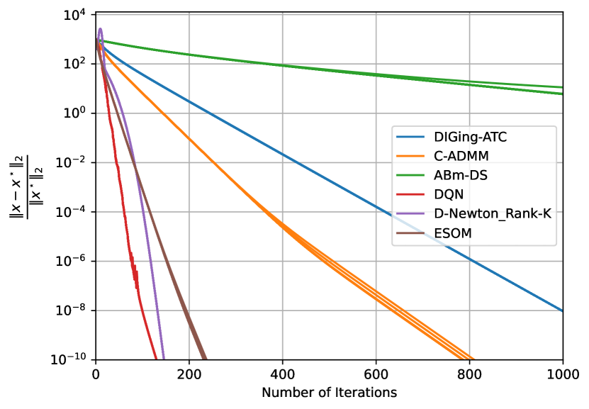
Figure 1: Convergence error of each agent per iteration in the distributed quadratic programming problem with a poorly-conditioned Hessian on a randomly-generated connected communication graph, with ${\kappa=0.569}$. The performance of DIGing-ATC and $ABm$-DS degrades notably in poorly-conditioned problems, compared to C-ADMM, DQN, and the second-order methods D-Newton Rank-$K$ and ESOM.

Further, we examine the performance of the distributed optimization methods on $20$ randomly-generated poorly-conditioned quadratic programs on different communication graphs, with the condition number of the aggregate Hessian ranging between $42.339$ and $172.149$. We initialize the estimate of the inverse Hessian of each agent’s local objective function to $0.1I_{n}$ in DQN, and further initialize ESOM-$K$ with ${\epsilon=0.1}$ and ${K=10}$. We do not include D-Newton Rank-$K$ in this evaluation, noting that D-Newton Rank-$K$ requires more than one order of magnitude greater computation time and about seven-times greater communication cost compared to the best-competing second-order method ESOM. In Table II, we provide the mean and standard deviation of the cumulative computation time and the cumulative size of the messages exchanged per agent in each algorithm. We compute the summary statistics over successful runs of each algorithm and provide the associated success rate of each algorithm in Table II. We display the best-performing stats in bold font, considering only algorithms that converge on all problems. We display entries associated with a success rate below $100\%$ in red. We note that only DQN and ESOM attain a $100\%$ success rate, converging to the optimal solution in all problems. In line with the preceding discussion, the first-order methods $ABm$-DS, DIGing-ATC, and C-ADMM attain low success rates, especially on sparsely-connected communication graphs. As noted in the Table II, DQN incurs the least communication cost across all values of the connectivity ratio $\kappa$, reducing the communication cost of ESOM by about seven-times. Moreover, DQN attains the fastest computation time across all values of $\kappa$, with the exception of ${\kappa=0.21}$, where ESOM attains a faster computation time. Even without a limit on the maximum number of iterations available to each algorithm for convergence, DQN still requires the least communication overhead in comparison to all other algorithms, including $ABm$-DS, DIGing-ATC, and C-ADMM, across all values of ${\kappa}$, except ${\kappa=0.21}$.

TABLE II: The mean and standard deviation of the cumulative computation time (Comp. Time), in seconds (secs.), and the cumulative size of messages exchanged per agent (Comm. Cost), in Megabytes (MB), in $20$ poorly-conditioned quadratic programs, across a range of communication networks, in addition to the success rate of each algorithm in converging to the optimal solution. Entries associated with a success rate below $100\%$ are displayed in red.

Algorithm $\bm{\kappa}=\bm{0.21}$ $\bm{\kappa}=\bm{0.57}$ Comp. Time (secs.) Comm. Cost (MB) Success Rate ($\%$) Comp. Time (secs.) Comm. Cost (MB) Success Rate ($\%$) $ABm$-DS [56] — — $0$ — — $0$ C-ADMM [35] $7.04\mathrm{e}^{-3}\pm 1.37\mathrm{e}^{-3}$ $2.49\mathrm{e}^{-1}\pm 4.23\mathrm{e}^{-2}$ $45$ $7.24\mathrm{e}^{-3}\pm 1.40\mathrm{e}^{-3}$ $2.51\mathrm{e}^{-1}\pm 4.27\mathrm{e}^{-2}$ $60$ DIGing-ATC [23] $5.90\mathrm{e}^{-3}$ $5.65\mathrm{e}^{-1}$ $5$ $4.62\mathrm{e}^{-3}\pm 7.63\mathrm{e}^{-4}$ $5.10\mathrm{e}^{-1}\pm 8.99\mathrm{e}^{-2}$ $15$ ESOM [46] $\bm{3.23\mathrm{e}^{-2}\pm 1.07\mathrm{e}^{-2}}$ $2.00\mathrm{e}^{0}\pm 3.36\mathrm{e}^{-1}$ $100$ $1.74\mathrm{e}^{-2}\pm 5.14\mathrm{e}^{-3}$ $1.10\mathrm{e}^{0}\pm 2.55\mathrm{e}^{-1}$ $100$ DQN (ours) $3.85\mathrm{e}^{-2}\pm 1.15\mathrm{e}^{-2}$ $\bm{4.10\mathrm{e}^{-1}\pm 1.19\mathrm{e}^{-1}}$ $100$ $\bm{1.63\mathrm{e}^{-2}\pm 4.14\mathrm{e}^{-3}}$ $\bm{1.61\mathrm{e}^{-1}\pm 2.45\mathrm{e}^{-2}}$ $100$

Algorithm $\bm{\kappa}=\bm{0.74}$ $\bm{\kappa}=\bm{0.85}$ Comp. Time (secs.) Comm. Cost (MB) Success Rate ($\%$) Comp. Time (secs.) Comm. Cost (MB) Success Rate ($\%$) $ABm$-DS [56] — — $0$ — — $0$ C-ADMM [35] $7.48\mathrm{e}^{-3}\pm 1.53\mathrm{e}^{-3}$ $2.58\mathrm{e}^{-1}\pm 4.38\mathrm{e}^{-2}$ $70$ $8.29\mathrm{e}^{-3}\pm 2.02\mathrm{e}^{-3}$ $2.58\mathrm{e}^{-1}\pm 4.58\mathrm{e}^{-2}$ $70$ DIGing-ATC [23] $4.84\mathrm{e}^{-3}\pm 9.70\mathrm{e}^{-4}$ $5.12\mathrm{e}^{-1}\pm 8.84\mathrm{e}^{-2}$ $20$ $5.27\mathrm{e}^{-3}\pm 9.30\mathrm{e}^{-4}$ $4.97\mathrm{e}^{-1}\pm 8.71\mathrm{e}^{-2}$ $20$ ESOM [46] $1.78\mathrm{e}^{-2}\pm 5.06\mathrm{e}^{-3}$ $1.08\mathrm{e}^{0}\pm 2.59\mathrm{e}^{-1}$ $100$ $1.94\mathrm{e}^{-2}\pm 8.21\mathrm{e}^{-3}$ $1.08\mathrm{e}^{0}\pm 2.34\mathrm{e}^{-1}$ $100$ DQN (ours) $\bm{1.37\mathrm{e}^{-2}\pm 3.07\mathrm{e}^{-3}}$ $\bm{1.52\mathrm{e}^{-1}\pm 4.01\mathrm{e}^{-2}}$ $100$ $\bm{1.27\mathrm{e}^{-2}\pm 4.75\mathrm{e}^{-3}}$ $\bm{1.48\mathrm{e}^{-1}\pm 3.26\mathrm{e}^{-2}}$ $100$

VII-B Logistic Regression

We examine the performance in non-quadratic problems, specifically logistic regression problems, which arise in a variety of domains. We consider the logistic regression problem:

$$\underset{x\in\mathbb{R}^{n}}{\mathrm{minimize}}\ \frac{\alpha}{2}\left\|x\right\|_{2}^{2}+\sum_{i=1}^{N}\sum_{j=1}^{m_{i}}\ln\left(1+\exp\left(-(a_{ij}^{\mathsf{T}}x)b_{ij}\right)\right),$$ (41)

where ${\alpha\in\mathbb{R}_{+}}$ denotes the weight of the regularization term (added to prevent overfitting), and $m_{i}$ denotes the number of training samples ${\{(a_{ij},b_{ij})\}_{j=1}^{m_{i}}}$ available to agent $i$, with ${a_{ij}\in\mathbb{R}^{n}}$ and ${b_{ij}\in\{-1,1\}}$ representing the binary labels. We note that each agent has access to only its local training samples. We consider a problem with ${N=50}$ agents, ${n=40}$, and ${\alpha=1\mathrm{e}^{-2}}$. We randomly generate the training samples, with $m_{i}$ sampled from the uniform distribution over the interval ${[5,30)}$.

We examine the performance of each algorithm on a randomly-generated connected communication graph with ${\kappa=0.569}$. We initialize D-Newton Rank-$K$ with ${\gamma=0.03}$, ${M=1}$, and ${K=25}$, with the number of communication rounds for the multi-step consensus procedure set at $15$. Likewise, we initialize ESOM-$K$ with ${\epsilon=1}$ and ${K=15}$. In DQN, we set the initial estimate of the inverse Hessian of each agent’s objective function to $1\mathrm{e}^{-2}I_{n}$. We note that a closed-form solution does not exist for C-ADMM, limiting the competitiveness of C-ADMM. Consequently, we do not include C-ADMM in this evaluation. We provide the cumulative computation time and cumulative size of messages exchanged per agent in Table III. While the first-order methods $ABm$-DS and DIGing-ATC fail to converge in this problem, DQN as well as the second-order methods D-Newton Rank-$K$ and ESOM converge to the optimal solution. Further, DQN attains the fastest computation time, while incurring the minimum communication cost. Despite using a poor guess as the initial estimate of the inverse Hessian in DQN, DQN still converges in about the same number of iterations as the second-order methods, as depicted in Figure 2. The first-order methods exhibit notably slower convergence rate in terms of the number of iterations compared to the other algorithms.

TABLE III: The cumulative computation time (in seconds), the cumulative size of messages exchanged per agent (in Megabytes), and the convergence status in the logistic regression problem, with ${\kappa=0.569}$.

Algorithm Computation Time (secs.) Messages Exchanged (MB) Converged $ABm$-DS [56] — — ✗ DIGing-ATC [23] — — ✗ D-Newton Rank-$K$ [15] $5.215\mathrm{e}^{-1}$ $7.392\mathrm{e}^{0}$ ✓ ESOM [46] $3.184\mathrm{e}^{-2}$ $9.683\mathrm{e}^{-1}$ ✓ DQN (ours) $\bm{1.246\mathrm{e}^{-2}}$ $\bm{1.478\mathrm{e}^{-1}}$ ✓

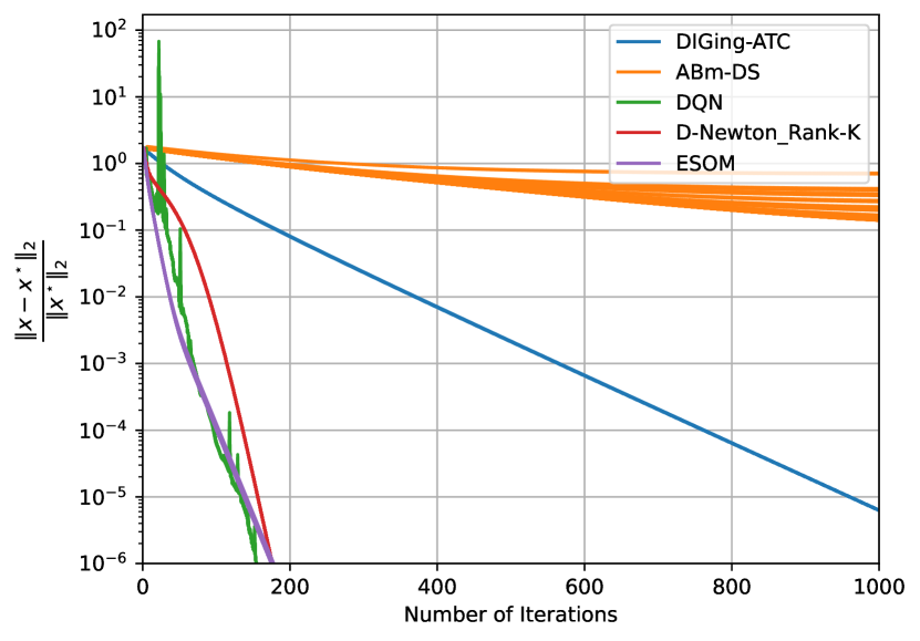
Figure 2: Per-iteration convergence error of each agent in the distributed logistic regression problem on a randomly-generated connected communication graph, with ${\kappa=0.569}$. While the first-order methods DIGing-ATC and $ABm$-DS exhibit slow convergence, DQN and the second-order methods D-Newton Rank-$K$ and ESOM converge faster.

In addition, we assess the performance across a range of communication networks, over $20$ logistic regression problems. We initialize each algorithm with the same parameters, retaining ESOM while dropping D-Newton Rank-$K$ in the evaluations. Table IV. While ESOM achieves the fastest computation time when ${\kappa=0.21}$, DQN achieves the fastest computation time for all other values of $\kappa$, compared to the other algorithms. Moreover, DQN and ESOM attain a perfect success rate, unlike the first-order methods. DQN incurs the least communication cost for convergence, even when each algorithm has an unlimited number of iterations available for convergence. Compared to ESOM, DQN incurs about an order of magnitude lower communication cost for all values of $\kappa$, with the exception of ${\kappa=0.21}$ where DQN reduces the communication cost by a factor of about four, relative to ESOM.

TABLE IV: The mean and standard deviation of the cumulative computation time (Comp. Time), in seconds (secs.), and the cumulative size of messages exchanged per agent (Comm. Cost), in Megabytes (MB), in $20$ logistic regression problems, across a range of communication networks, in addition to the success rate of each algorithm in converging to the optimal solution. Entries associated with a success rate below $100\%$ are displayed in red.

Algorithm $\bm{\kappa}=\bm{0.21}$ $\bm{\kappa}=\bm{0.57}$ Comp. Time (secs.) Comm. Cost (MB) Success Rate ($\%$) Comp. Time (secs.) Comm. Cost (MB) Success Rate ($\%$) $ABm$-DS [56] — — $0$ — — $0$ DIGing-ATC [23] $3.25\mathrm{e}^{-2}\pm 8.56\mathrm{e}^{-3}$ $5.62\mathrm{e}^{-1}\pm 7.55\mathrm{e}^{-2}$ $40$ $2.89\mathrm{e}^{-2}\pm 6.19\mathrm{e}^{-3}$ $5.02\mathrm{e}^{-1}\pm 8.24\mathrm{e}^{-2}$ $85$ ESOM [46] $\bm{2.60\mathrm{e}^{-2}\pm 1.69\mathrm{e}^{-2}}$ $1.17\mathrm{e}^{0}\pm 8.09\mathrm{e}^{-1}$ $100$ $2.31\mathrm{e}^{-2}\pm 1.44\mathrm{e}^{-2}$ $1.16\mathrm{e}^{0}\pm 8.59\mathrm{e}^{-1}$ $100$ DQN (ours) $3.91\mathrm{e}^{-2}\pm 1.40\mathrm{e}^{-2}$ $\bm{2.72\mathrm{e}^{-1}\pm 1.28\mathrm{e}^{-1}}$ $100$ $\bm{1.84\mathrm{e}^{-2}\pm 5.19\mathrm{e}^{-3}}$ $\bm{1.18\mathrm{e}^{-1}\pm 3.85\mathrm{e}^{-2}}$ $100$

Algorithm $\bm{\kappa}=\bm{0.74}$ $\bm{\kappa}=\bm{0.85}$ Comp. Time (secs.) Comm. Cost (MB) Success Rate ($\%$) Comp. Time (secs.) Comm. Cost (MB) Success Rate ($\%$) $ABm$-DS [56] — — $0$ — — $0$ DIGing-ATC [23] $2.68\mathrm{e}^{-2}\pm 8.49\mathrm{e}^{-3}$ $4.99\mathrm{e}^{-1}\pm 1.10\mathrm{e}^{-1}$ $95$ $2.48\mathrm{e}^{-2}\pm 7.31\mathrm{e}^{-3}$ $4.64\mathrm{e}^{-1}\pm 1.18\mathrm{e}^{-1}$ $85$ ESOM [46] $2.42\mathrm{e}^{-2}\pm 1.42\mathrm{e}^{-2}$ $1.16\mathrm{e}^{0}\pm 7.78\mathrm{e}^{-1}$ $100$ $2.33\mathrm{e}^{-2}\pm 1.38\mathrm{e}^{-2}$ $1.15\mathrm{e}^{0}\pm 7.62\mathrm{e}^{-1}$ $100$ DQN (ours) $\bm{1.65\mathrm{e}^{-2}\pm 4.85\mathrm{e}^{-3}}$ $\bm{1.06\mathrm{e}^{-1}\pm 1.60\mathrm{e}^{-2}}$ $100$ $\bm{1.63\mathrm{e}^{-2}\pm 6.13\mathrm{e}^{-3}}$ $\bm{1.04\mathrm{e}^{-1}\pm 2.35\mathrm{e}^{-2}}$ $100$

VIII Numerical Evaluations of EC-DQN

We evaluate the performance of EC-DQN, in comparison to existing distributed algorithms for multi-agent constrained optimization, including consensus ADMM (C-ADMM) [35], SONATA [27], and DPDA [34]. In our evaluations, we consider equality-constrained basis pursuit denoising and logistic regression problems across communication networks with different connectivity ratios ${\kappa}$. We utilize the same evaluation setup as in Section VII. The update procedures in C-ADMM and SONATA require each agent to solve an optimization problem, adversely affecting the computation time of each agent if these problems are solved exactly. To ensure that these methods remain competitive to other algorithms with respect to the computation time, we solve the pertinent optimization problems inexactly using sequential quadratic programming techniques. Empirical results indicate that the inexact updates did not have a material effect on the convergence rates of these algorithms.

VIII-A Basis Pursuit Denoising

We consider the following optimization problem:

$$\underset{x\in\mathbb{R}^{n}}{\mathrm{minimize}} \sum_{i=1}^{N}\frac{1}{2}\left\|A_{i}x-b_{i}\right\|_{2}^{2}+\lambda\left\|x\right\|_{1}$$ (42)

$$\mathrm{subject\ to\ } Fx=e,$$

where ${A_{i}\in\mathbb{R}^{p_{i}\times n}}$, ${b_{i}\in\mathbb{R}^{p_{i}}}$ represent the local data only available to agent $i$. Moreover, each agent has access to ${(F\in\mathbb{R}^{m\times n},e\in\mathbb{R}^{m})}$ defining the constraints in the optimization problem. The parameter $\lambda$ determines the relative weighting between the reconstruction quality associated with the $\ell_{2}^{2}$-norm and sparsity of the solution associated with the $\ell_{1}$-norm. Problems of this form arise in a variety of applications such as image compression, compressed sensing, and least absolute shrinkage and selection operator (LASSO) regression. Similar problems also arise in sparse dictionary learning. We consider a multi-agent setting with ${N=50}$ agents, ${n=40}$, and ${\lambda=1\mathrm{e}^{-2}}$. We randomly generate the problem data available to each agent, including the number of constraints, such that the rank of ${A_{i}<n}$, ${\forall i\in\mathcal{V}}$. We execute each algorithm for a maximum of $1000$ iterations, with a convergence threshold of $1\mathrm{e}^{-8}$. We initialize each agent’s estimate of the Hessian of the problem to a randomly-generated positive-definite symmetric matrix in EC-DQN. Due to space constraints, we consider poorly-conditioned basis problems here and provide the results in well-conditioned problem settings in the Supplemental Material.

We begin by examining the performance of each algorithm in $20$ well-conditioned optimization problems on randomly-generated communication networks, with ${\kappa}$ varying from $0.219$ to $0.856$ and condition number of the Hessian ranging between $2.578$ and $2.097$. We present the computation time and associated communication cost required for convergence per agent in each algorithm in Table V. When ${\kappa=0.22}$, SONATA achieves the fastest computation time, while C-ADMM requires the least communication cost for convergence to the optimal solution. However, for all other values of $\kappa$, EC-DQN attains the fastest computation time, while incurring the least communication cost for convergence. In these problems, C-ADMM requires a notably greater computation time relative to the other algorithms. DPDA fails to converge to the desired convergence threshold within the maximum number of iterations. In Figure 3, we examine the performance of each algorithm on a problem with condition number $2.312$ and a communication graph with ${\kappa=0.578}$. We note that EC-DQN requires the fewest number of iterations for convergence to the optimal solution. Further, EC-DQN attains the fastest computation time and least communication cost of $3.17\mathrm{e}^{-2}$ secs. and $8.81\mathrm{e}^{-3}$ MB, respectively, compared to the best-competing algorithm SONATA with a computation time and communication cost of $8.52\mathrm{e}^{-2}$ secs. and $2.32\mathrm{e}^{-2}$ MB, respectively. Although the convergence error of the agents’ iterates in DPDA decreases at each iteration, it does not decrease fast enough to attain convergence within $1000$ iterations. C-ADMM, however, converges in about $400$ iterations.

TABLE V: The mean and standard deviation of the cumulative computation time (Comp. Time), in seconds (secs.), and communication cost (Comm. Cost), in Megabytes (MB), per agent, in $20$ well-conditioned basis pursuit denoising problems, on different communication networks.

Algorithm	$\bm{\kappa}=\bm{0.22}$		$\bm{\kappa}=\bm{0.57}$
	Comp. Time (secs.)	Comm. Cost (MB)	Comp. Time (secs.)	Comm. Cost (MB)
C-ADMM [35]	$2.73\mathrm{e}^{-2}\pm 1.32\mathrm{e}^{-2}$	$\bm{7.93\mathrm{e}^{-2}\pm 4.23\mathrm{e}^{-2}}$	$3.44\mathrm{e}^{-2}\pm 1.91\mathrm{e}^{-2}$	$8.93\mathrm{e}^{-2}\pm 4.36\mathrm{e}^{-2}$
DPDA [34]	—	—	—	—
SONATA [27]	$\bm{1.74\mathrm{e}^{-2}\pm 4.62\mathrm{e}^{-3}}$	$9.80\mathrm{e}^{-2}\pm 3.94\mathrm{e}^{-2}$	$6.72\mathrm{e}^{-3}\pm 2.13\mathrm{e}^{-3}$	$4.61\mathrm{e}^{-2}\pm 1.80\mathrm{e}^{-2}$
EC-DQN (ours)	$1.91\mathrm{e}^{-2}\pm 5.60\mathrm{e}^{-3}$	$1.28\mathrm{e}^{-1}\pm 1.72\mathrm{e}^{-2}$	$\bm{4.95\mathrm{e}^{-3}\pm 1.55\mathrm{e}^{-3}}$	$\bm{3.24\mathrm{e}^{-2}\pm 3.32\mathrm{e}^{-3}}$

Algorithm	$\bm{\kappa}=\bm{0.75}$		$\bm{\kappa}=\bm{0.86}$
	Comp. Time (secs.)	Comm. Cost (MB)	Comp. Time (secs.)	Comm. Cost (MB)
C-ADMM [35]	$2.83\mathrm{e}^{-2}\pm 1.39\mathrm{e}^{-2}$	$7.67\mathrm{e}^{-2}\pm 3.65\mathrm{e}^{-2}$	$2.49\mathrm{e}^{-2}\pm 1.41\mathrm{e}^{-2}$	$6.96\mathrm{e}^{-2}\pm 3.54\mathrm{e}^{-2}$
DPDA [34]	—	—	—	—
SONATA [27]	$5.29\mathrm{e}^{-3}\pm 2.30\mathrm{e}^{-3}$	$3.20\mathrm{e}^{-2}\pm 1.10\mathrm{e}^{-2}$	$7.08\mathrm{e}^{-3}\pm 3.87\mathrm{e}^{-3}$	$4.23\mathrm{e}^{-2}\pm 2.12\mathrm{e}^{-2}$
EC-DQN (ours)	$\bm{3.71\mathrm{e}^{-3}\pm 1.08\mathrm{e}^{-3}}$	$\bm{2.27\mathrm{e}^{-2}\pm 2.61\mathrm{e}^{-3}}$	$\bm{3.39\mathrm{e}^{-3}\pm 8.60\mathrm{e}^{-4}}$	$\bm{2.40\mathrm{e}^{-2}\pm 3.87\mathrm{e}^{-3}}$

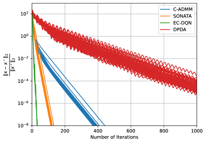
Figure 3: Convergence error of each algorithm on a randomly-generated communication graph with ${\kappa=0.566}$ in a well-conditioned basis pursuit denoising problem. EC-DQN converges faster than all methods.

Further, we examine the performance of each algorithm in poorly-conditioned basis pursuit denoising problems, with the condition number ranging between $53.895$ and $125.029$, on randomly-generated communication networks with different connectivity ratios. Table VI summarizes the performance of each algorithm in these problems, highlighting the cumulative computation time and communication cost on $20$ instances of such problems. Similar to the results obtained in the well-conditioned problem setting, when ${\kappa=0.22}$, C-ADMM attains the least communication cost, with SONATA achieving the fastest computation time for convergence. Although at ${\kappa=0.22}$, we note that all algorithms achieve similar performance in terms of computation time and communication cost. For all other values of $\kappa$, EC-DQN converges the fastest, while requiring the least communication overhead. Further, the performance of DPDA degrades notably, as illustrated in Figure 4. In Figure 4, we show the performance of each algorithm on an instance of the problems with ${\kappa=0.566}$ and a condition number of $99.698$. In this problem, EC-DQN and C-ADMM incur the least communication cost, requiring $5.19\mathrm{e}^{-2}$ MB for convergence. However, EC-DQN attains the fastest computation time of $1.43\mathrm{e}^{-2}$ secs., compared to the second-fastest method SONATA, which requires $2.33\mathrm{e}^{-2}$ secs. and a communication cost of $9.28\mathrm{e}^{-2}$ MB. C-ADMM requires $2.51\mathrm{e}^{-2}$ secs. for convergence. Further, we note that C-ADMM, SONATA, and EC-DQN converged on all problem instances, in the well-conditioned and poorly-conditioned settings.

TABLE VI: The mean and standard deviation of the cumulative computation time (Comp. Time), in seconds (secs.), and communication cost (Comm. Cost), in Megabytes (MB), per agent, in $20$ poorly-conditioned basis pursuit denoising problems, on different communication networks.

Algorithm	$\bm{\kappa}=\bm{0.22}$		$\bm{\kappa}=\bm{0.57}$
	Comp. Time (secs.)	Comm. Cost (MB)	Comp. Time (secs.)	Comm. Cost (MB)
C-ADMM [35]	$4.67\mathrm{e}^{-2}\pm 1.28\mathrm{e}^{-2}$	$\bm{1.35\mathrm{e}^{-1}\pm 3.09\mathrm{e}^{-2}}$	$4.33\mathrm{e}^{-2}\pm 1.53\mathrm{e}^{-2}$	$1.27\mathrm{e}^{-1}\pm 4.05\mathrm{e}^{-2}$
DPDA [34]	—	—	—	—
SONATA [27]	$\bm{2.85\mathrm{e}^{-2}\pm 1.09\mathrm{e}^{-2}}$	$1.76\mathrm{e}^{-1}\pm 7.01\mathrm{e}^{-2}$	$1.73\mathrm{e}^{-2}\pm 7.70\mathrm{e}^{-3}$	$1.34\mathrm{e}^{-1}\pm 7.50\mathrm{e}^{-2}$
EC-DQN (ours)	$2.88\mathrm{e}^{-2}\pm 8.44\mathrm{e}^{-3}$	$1.89\mathrm{e}^{-1}\pm 3.65\mathrm{e}^{-2}$	$\bm{9.99\mathrm{e}^{-3}\pm 2.21\mathrm{e}^{-3}}$	$\bm{6.92\mathrm{e}^{-2}\pm 2.26\mathrm{e}^{-2}}$

Algorithm	$\bm{\kappa}=\bm{0.75}$		$\bm{\kappa}=\bm{0.86}$
	Comp. Time (secs.)	Comm. Cost (MB)	Comp. Time (secs.)	Comm. Cost (MB)
C-ADMM [35]	$4.03\mathrm{e}^{-2}\pm 1.56\mathrm{e}^{-2}$	$1.21\mathrm{e}^{-1}\pm 4.26\mathrm{e}^{-2}$	$4.24\mathrm{e}^{-2}\pm 1.82\mathrm{e}^{-2}$	$1.22\mathrm{e}^{-1}\pm 4.56\mathrm{e}^{-2}$
DPDA [34]	—	—	—	—
SONATA [27]	$1.44\mathrm{e}^{-2}\pm 5.35\mathrm{e}^{-3}$	$1.11\mathrm{e}^{-1}\pm 6.60\mathrm{e}^{-2}$	$1.36\mathrm{e}^{-2}\pm 6.95\mathrm{e}^{-3}$	$1.16\mathrm{e}^{-1}\pm 7.94\mathrm{e}^{-2}$
EC-DQN (ours)	$\bm{7.36\mathrm{e}^{-3}\pm 1.67\mathrm{e}^{-3}}$	$\bm{5.25\mathrm{e}^{-2}\pm 1.83\mathrm{e}^{-2}}$	$\bm{7.51\mathrm{e}^{-3}\pm 3.14\mathrm{e}^{-3}}$	$\bm{5.32\mathrm{e}^{-2}\pm 1.86\mathrm{e}^{-2}}$

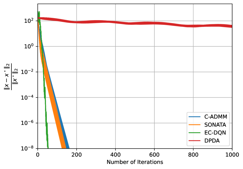
Figure 4: Convergence error of each algorithm in a poorly-conditioned basis pursuit denoising problem, on a randomly-generated communication graph with ${\kappa=0.566}$. EC-DQN achieves the fastest convergence rate compared to the other algorithms.

VIII-B Logistic Regression

In addition, we evaluate each algorithm in constrained logistic regression problems, expressed in the form:

$$\underset{x\in\mathbb{R}^{n}}{\mathrm{minimize}} \frac{\alpha}{2}\left\|x\right\|_{2}^{2}+\sum_{i=1}^{N}\sum_{j=1}^{m_{i}}\ln\left(1+\exp\left(-(a_{ij}^{\mathsf{T}}x)b_{ij}\right)\right),$$ (43)

$$\mathrm{subject\ to\ } Fx=e,$$

where ${\{(a_{ij},b_{ij})\}_{j=1}^{m_{i}}}$ denotes the training data available to agent $i$ and $m_{i}$ denotes the number of training data samples, with regularization parameter ${\alpha\in\mathbb{R}_{+}}$, ${F\in\mathbb{R}^{m\times n}}$, and ${e\in\mathbb{R}^{m}}$. We consider the problem in (43) with ${N=50}$ agents and ${n=40}$. Further, we randomly generate the problem data, the communication networks, and each agent’s estimate of the Hessian of the problem. We utilize a convergence threshold of $1\mathrm{e}^{-7}$, with ${\alpha=1\mathrm{e}^{-2}}$ and the maximum number of iterations set at $1000$.

In Table VII, we summarize the performance of each algorithm on $20$ instances of the logistic regression problem, noting the total computation time and communication cost per agent required by each algorithm for convergence on different communication graphs. As presented in Table VII, EC-DQN achieves the fastest computation time and least communication cost across all communication networks, except at ${\kappa=0.22}$ where C-ADMM attains the minimum communication cost. We note that, on each communication graph, C-ADMM failed to converge in one problem, whereas EC-DQN and SONATA converged in all cases. When an algorithm fails to converge, we do not utilize the computation time and communication cost for that run in computing the summary statistics for that algorithm. Figure 5 depicts the convergence rate of each algorithm per iteration on an instance of (43) with ${\kappa=0.566}$. We note that EC-DQN converges within the fewest number of iterations. Moreover, EC-DQN requires the least communication cost of ${2.50\mathrm{e}^{-2}}$ MB with the fastest computation time ($8.00\mathrm{e}^{-3}$ secs.) for convergence. In this problem, SONATA requires a computation time and communication cost of $2.49\mathrm{e}^{-2}$ secs. and $6.15\mathrm{e}^{-2}$ MB, respectively, outperforming C-ADMM, which requires a computation time and communication cost of $4.49\mathrm{e}^{-2}$ secs. and $6.56\mathrm{e}^{-2}$ MB, respectively. DPDA fails to converge within $1000$ iterations.

TABLE VII: The mean and standard deviation of the cumulative computation time (Comp. Time), in seconds (secs.), and communication cost (Comm. Cost), in Megabytes (MB), per agent, in $20$ constrained logistic regression problems, on different communication networks.

Algorithm	$\bm{\kappa}=\bm{0.22}$		$\bm{\kappa}=\bm{0.57}$
	Comp. Time (secs.)	Comm. Cost (MB)	Comp. Time (secs.)	Comm. Cost (MB)
C-ADMM [35]	$4.05\mathrm{e}^{-2}\pm 2.74\mathrm{e}^{-2}$	$\bm{7.86\mathrm{e}^{-2}\pm 4.31\mathrm{e}^{-2}}$	$3.95\mathrm{e}^{-2}\pm 2.06\mathrm{e}^{-2}$	$7.70\mathrm{e}^{-2}\pm 4.25\mathrm{e}^{-2}$
DPDA [34]	—	—	—	—
SONATA [27]	$3.81\mathrm{e}^{-2}\pm 1.64\mathrm{e}^{-2}$	$1.80\mathrm{e}^{-1}\pm 1.17\mathrm{e}^{-1}$	$2.88\mathrm{e}^{-2}\pm 1.22\mathrm{e}^{-2}$	$1.39\mathrm{e}^{-1}\pm 8.82\mathrm{e}^{-2}$
EC-DQN (ours)	$\bm{2.41\mathrm{e}^{-2}\pm 1.16\mathrm{e}^{-2}}$	$1.43\mathrm{e}^{-1}\pm 4.43\mathrm{e}^{-2}$	$\bm{5.79\mathrm{e}^{-3}\pm 3.89\mathrm{e}^{-3}}$	$\bm{4.13\mathrm{e}^{-2}\pm 3.37\mathrm{e}^{-2}}$

Algorithm	$\bm{\kappa}=\bm{0.75}$		$\bm{\kappa}=\bm{0.86}$
	Comp. Time (secs.)	Comm. Cost (MB)	Comp. Time (secs.)	Comm. Cost (MB)
C-ADMM [35]	$4.03\mathrm{e}^{-2}\pm 2.19\mathrm{e}^{-2}$	$7.95\mathrm{e}^{-2}\pm 4.71\mathrm{e}^{-2}$	$4.51\mathrm{e}^{-2}\pm 2.41\mathrm{e}^{-2}$	$7.90\mathrm{e}^{-2}\pm 3.84\mathrm{e}^{-2}$
DPDA [34]	—	—	—	—
SONATA [27]	$2.80\mathrm{e}^{-2}\pm 1.44\mathrm{e}^{-2}$	$1.37\mathrm{e}^{-1}\pm 1.01\mathrm{e}^{-1}$	$2.51\mathrm{e}^{-2}\pm 1.24\mathrm{e}^{-2}$	$1.23\mathrm{e}^{-1}\pm 7.85\mathrm{e}^{-2}$
EC-DQN (ours)	$\bm{5.57\mathrm{e}^{-3}\pm 4.14\mathrm{e}^{-3}}$	$\bm{3.66\mathrm{e}^{-2}\pm 3.58\mathrm{e}^{-2}}$	$\bm{4.95\mathrm{e}^{-3}\pm 3.08\mathrm{e}^{-3}}$	$\bm{2.89\mathrm{e}^{-2}\pm 2.12\mathrm{e}^{-2}}$

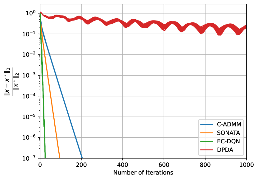
Figure 5: Convergence error of each algorithm in constrained logistic regression problems with ${\kappa=0.566}$. EC-DQN converges the fastest in comparison to the other algorithms.

IX Conclusion

We introduce distributed quasi-Newton algorithms: DQN—for unconstrained optimization—and EC-DQN—for equality-constrained optimization—that enable a group of agents to solve multi-agent optimization problems using an estimate of the curvature of the objective function of the problem. In our algorithms, each agent estimates the curvature of the objective function using its local gradients, while communicating with its immediate, one-hop neighbors over a communication network. Our algorithms converge to a stationary point of the optimization problem and provide faster empirical convergence in unconstrained and constrained problems, particularly in ill-conditioned problem settings, where distributed first-order methods show slow convergence rates. Moreover, our algorithm avoids the significant computation and communication overhead associated with existing distributed second-order and quasi-Newton methods by eschewing exact computation of the Hessian of the problem, in addition to estimating the inverse Hessian directly, making it amenable to problems where computation of the Hessian of the objective function is impractical or impossible. Future work will analyze the convergence rates of the proposed algorithms, noting that the numerical evaluations suggest superlinear convergence. In addition, future work will examine the extension of the proposed algorithms to convex inequality-constrained optimization problems, and more generally, non-convex constrained optimization problems, which arise in many applications.

Appendix

A Proof of Lemma 1

We prove convergence of the sequence ${\{\overline{\bm{x}}^{(k)}\}_{\forall k\geq 0}}$ to a limit point. Before proceeding, we introduce the following notation: We denote the mean step-size at iteration $k$ by ${\overline{\bm{\alpha}}^{(k)}\in\mathbb{R}^{N\times N}}$, a diagonal matrix with ${\overline{\bm{\alpha}}^{(k)}_{ii}=\frac{1}{N}\sum_{j\in\mathcal{V}}\alpha_{j}^{(k)}}$, ${\forall i\in\mathcal{V}}$, and, further, define ${r_{\alpha}=\alpha_{\max}\max_{k\geq 0}\frac{1}{\left\|\overline{\bm{\alpha}}^{(k)}\right\|_{2}}}$, where ${\alpha_{\max}=\max_{k\geq 0}\left\{\left\|\bm{\alpha}^{(k)}\right\|_{2}\right\}}$. In addition, from (16), (17), and (18), we obtain the following sequences:

$$\overline{\bm{x}}^{(k+1)} =\overline{\bm{x}}^{(k)}+\overline{\bm{\alpha}^{(k)}\bm{z}^{(k)}}$$ (44)

$$\overline{\bm{v}}^{(k+1)} =\overline{\bm{v}}^{(k)}+\overline{\bm{g}}^{(k+1)}-\overline{\bm{g}}^{(k)}$$ (45)

$$\overline{\bm{z}}^{(k+1)} =-\frac{\bm{1}_{N}\bm{1}_{N}^{\mathsf{T}}}{N}\bm{d}^{(k+1)}.$$ (46)

The following lemma bounds the disagreement error between the iterates of each agent and the mean of all the agents’ iterates. We omit the proof here, noting that the proof follows along the same lines as that in [53].

Lemma 2.

The sequences $\{\tilde{\bm{x}}^{(k)}\}_{\forall k\geq 0}$, $\{\tilde{\bm{v}}^{(k)}\}_{\forall k\geq 0}$, and $\{\tilde{\bm{z}}^{(k)}\}_{\forall k\geq 0}$, representing the disagreement between the agents on their corresponding local variables satisfy the following bounds:

$$\left\|\tilde{\bm{x}}^{(k+1)}\right\|_{2} \leq\lambda\left\|\tilde{\bm{x}}^{(k)}\right\|_{2}+\lambda r_{\alpha}\left\|\overline{\bm{\alpha}^{(k)}\bm{z}^{(k)}}\right\|_{2}$$

$$\quad+\lambda^{2}\alpha_{\max}(1+r_{\alpha})q\left(\left\|\tilde{\bm{v}}^{(k)}\right\|_{2}+\left\|\overline{\bm{g}}^{(k)}\right\|_{2}\right),$$ (47)

$$\left\|\tilde{\bm{v}}^{(k+1)}\right\|_{2} \leq\left(\lambda+\lambda^{3}L\alpha_{\max}(1+r_{\alpha})q\right)\left\|\tilde{\bm{v}}^{(k)}\right\|_{2}$$

$$\quad+\lambda L(1+\lambda)\left\|\tilde{\bm{x}}^{(k)}\right\|_{2}$$

$$\quad+\lambda^{3}L\alpha_{\max}(1+r_{\alpha})q\left\|\overline{\bm{g}}^{(k)}\right\|_{2}$$

$$\quad+\lambda L(1+\lambda r_{\alpha})\left\|\overline{\bm{\alpha}^{(k)}\bm{z}^{(k)}}\right\|_{2},$$ (48)

$$\left\|\tilde{\bm{z}}^{(k+1)}\right\|_{2} \leq\lambda q\left(\left\|\tilde{\bm{v}}^{(k+1)}\right\|_{2}+\left\|\overline{\bm{g}}^{(k+1)}\right\|_{2}\right),$$ (49)

respectively, given the recurrence in (19), (12), (20), where ${q^{2}=\min\{n,N\}}$.

Upon defining the following sequences:

$$X^{(k)} =\sqrt{\sum_{l=0}^{k}\left\|\tilde{\bm{x}}^{(l)}\right\|_{2}^{2}},\quad V^{(k)}=\sqrt{\sum_{l=0}^{k}\left\|\tilde{\bm{v}}^{(l)}\right\|_{2}^{2}},$$ (50)

$$R^{(k)} =\sqrt{\sum_{l=0}^{k}\left(\left\|\overline{\bm{\alpha}^{(l)}\bm{z}^{(l)}}\right\|_{2}^{2}+\left\|\tilde{\bm{g}}^{(l+1)}\right\|_{2}^{2}\right)},$$ (51)

we obtain the following bounds on $X^{(k)}$ and $V^{(k)}$ from Lemma 2:

$$X^{(k)}\leq\mu_{xr}R^{(k)}+\mu_{xc},$$ (52)

$$V^{(k)}\leq\theta_{vr}R^{(k)}+\theta_{vc},$$ (53)

where ${\mu_{xr}=\frac{\rho_{xr}+\rho_{xv}\rho_{vr}}{\eta}}$, ${\mu_{xc}=\frac{\rho_{xv}\epsilon_{v}+\epsilon}{\eta}}$, ${\theta_{vr}=\frac{\rho_{vx}\rho_{xr}+\rho_{vr}}{\eta}}$, ${\theta_{vc}=\frac{\rho_{vx}\epsilon{x}+\epsilon_{v}}{\eta}}$, ${\eta=1-\rho_{vx}\rho_{xv}}$, with ${\rho_{xv}=\frac{\sqrt{2}}{1-\lambda}\lambda^{2}\alpha_{\max}(1+r_{\alpha})q}$, ${\rho_{vx}=\frac{\sqrt{2}}{1-\lambda}\lambda L(1+\lambda)}$, ${\rho_{xr}=\frac{\sqrt{2}}{1-\lambda}\left(\lambda^{2}\alpha_{\max}(1+r_{\alpha})q+\lambda r_{\alpha}\right)}$, ${\rho_{vr}=\frac{\sqrt{2}}{1-\lambda}\left(\lambda^{3}L\alpha_{\max}(1+r_{\alpha})q+\lambda L(1+\lambda r_{\alpha})\right)}$, ${\epsilon_{x}=\left\|\tilde{\bm{x}}^{(0)}\right\|_{2}\sqrt{\frac{2}{1-\lambda^{2}}}}$, and ${\epsilon_{v}=\left\|\tilde{\bm{v}}^{(0)}\right\|_{2}\sqrt{\frac{2}{1-\lambda^{2}}}}$.

Further, the following relation:

$$\bm{f}(\overline{\bm{x}}^{(k+1)}) \leq\bm{f}(\overline{\bm{x}}^{(k)})+\frac{1}{2}\left(\left\|\overline{\bm{g}}^{(k)}\right\|_{2}^{2}+\left\|\overline{\bm{\alpha}^{(k)}\bm{z}^{(k)}}\right\|_{2}^{2}\right)$$ (54)

$$\quad+\frac{L}{2}\left\|\overline{\bm{\alpha}^{(k)}\bm{z}^{(k)}}\right\|_{2}^{2}+L\left\|\tilde{\bm{x}}^{(k)}\right\|_{2}\left\|\overline{\bm{\alpha}^{(k)}\bm{z}^{(k)}}\right\|_{2}$$

results from $L$-Lipschitz continuity of the gradient of $f_{i}$, ${\forall i\in\mathcal{V}}$, which reduces to:

$$\bm{f}(\overline{\bm{x}}^{(t+1)}) \leq\bm{f}(\overline{\bm{x}}^{(0)})+\frac{1}{2}(1+L)\left(R^{(t)}\right)^{2}+LX^{(t)}R^{(t)},$$ (55)

by summing over $k$ from $0$ to $t$.

Using (52), we obtain:

$$\bm{f}(\overline{\bm{x}}^{(t+1)})\leq\bm{f}(\overline{\bm{x}}^{(0)})+a\left(R^{(t)}\right)^{2}+bR^{(t)},$$ (56)

where ${a=\frac{1}{2}(1+L)+L\mu_{xr}}$ and ${b=L\mu_{xc}}$.

Following the same procedure as the proof in [53], we obtain the following relation:

$$\lim_{t\rightarrow\infty}R^{(t)}\leq\frac{b+\sqrt{b^{2}-4a\left(\bm{f}(\overline{\bm{x}}^{(0)})-f^{\star}\right)}}{-2a}=\Sigma<\infty.$$ (57)

Applying the monotone convergence theorem, we note that:

$$\lim_{k\rightarrow\infty}\left(\left\|\overline{\bm{g}}^{(k)}\right\|_{2}^{2}+\left\|\overline{\bm{\alpha}^{(k)}\bm{z}^{(k)}}\right\|_{2}^{2}\right)=0,$$ (58)

which shows that:

$$\lim_{k\rightarrow\infty}\left\|\overline{\bm{g}}^{(k)}\right\|_{2}=\lim_{k\rightarrow\infty}\left\|\overline{\bm{\alpha}^{(k)}\bm{z}^{(k)}}\right\|_{2}=0,$$ (59)

and in addition:

$$\lim_{k\rightarrow\infty}\left\|\overline{\bm{x}}^{(k+1)}-\overline{\bm{x}}^{(k)}\right\|_{2}=0.$$ (60)

B Proof of Theorem 1

The proof of Lemma 1 follows from (52) and (53). From (57), we note that:

$$\lim_{k\rightarrow\infty}\left\|\tilde{\bm{x}}^{(k)}\right\|_{2}=0,\ \lim_{k\rightarrow\infty}\left\|\tilde{\bm{v}}^{(k)}\right\|_{2}=0,$$ (61)

since ${\lim_{k\rightarrow\infty}X^{(k)}<\infty}$ and ${\lim_{k\rightarrow\infty}X^{(k)}<\infty}$. Further, ${\lim_{k\rightarrow\infty}\left\|\tilde{\bm{z}}^{(k)}\right\|_{2}=0}$.

References

- [1] M. Bashir, S. Longtin-Martel, R. M. Botez, and T. Wong, “Aerodynamic design optimization of a morphing leading edge and trailing edge airfoil–application on the uas-s45,” Applied Sciences, vol. 11, no. 4, p. 1664, 2021.
- [2] M. Masdari, M. Tahani, M. H. Naderi, and N. Babayan, “Optimization of airfoil based savonius wind turbine using coupled discrete vortex method and salp swarm algorithm,” Journal of Cleaner Production, vol. 222, pp. 47–56, 2019.
- [3] V. Harish and A. Kumar, “Reduced order modeling and parameter identification of a building energy system model through an optimization routine,” Applied Energy, vol. 162, pp. 1010–1023, 2016.
- [4] I. Ahmadianfar, W. Gong, A. A. Heidari, N. A. Golilarz, A. Samadi-Koucheksaraee, and H. Chen, “Gradient-based optimization with ranking mechanisms for parameter identification of photovoltaic systems,” Energy Reports, vol. 7, pp. 3979–3997, 2021.
- [5] W. Long, T. Wu, M. Xu, M. Tang, and S. Cai, “Parameters identification of photovoltaic models by using an enhanced adaptive butterfly optimization algorithm,” Energy, vol. 229, p. 120750, 2021.
- [6] C. Toumieh and A. Lambert, “Decentralized multi-agent planning using model predictive control and time-aware safe corridors,” IEEE Robotics and Automation Letters, vol. 7, no. 4, pp. 11 110–11 117, 2022.
- [7] A. Torreno, E. Onaindia, and O. Sapena, “Fmap: Distributed cooperative multi-agent planning,” Applied Intelligence, vol. 41, pp. 606–626, 2014.
- [8] S. Mishra, C. Bordin, A. Tomasgard, and I. Palu, “A multi-agent system approach for optimal microgrid expansion planning under uncertainty,” International Journal of Electrical Power & Energy Systems, vol. 109, pp. 696–709, 2019.
- [9] G. Franzè, W. Lucia, and F. Tedesco, “A distributed model predictive control scheme for leader–follower multi-agent systems,” International Journal of Control, vol. 91, no. 2, pp. 369–382, 2018.
- [10] P. Wang and B. Ding, “A synthesis approach of distributed model predictive control for homogeneous multi-agent system with collision avoidance,” International Journal of Control, vol. 87, no. 1, pp. 52–63, 2014.
- [11] R. Luo, R. Bourdais, T. J. van den Boom, and B. De Schutter, “Multi-agent model predictive control based on resource allocation coordination for a class of hybrid systems with limited information sharing,” Engineering Applications of Artificial Intelligence, vol. 58, pp. 123–133, 2017.
- [12] I. Lobel and A. Ozdaglar, “Distributed subgradient methods for convex optimization over random networks,” IEEE Transactions on Automatic Control, vol. 56, no. 6, pp. 1291–1306, 2010.
- [13] C. Xi, R. Xin, and U. A. Khan, “ADD-OPT: Accelerated distributed directed optimization,” IEEE Transactions on Automatic Control, vol. 63, no. 5, pp. 1329–1339, 2017.
- [14] C. Xi, V. S. Mai, R. Xin, E. H. Abed, and U. A. Khan, “Linear convergence in optimization over directed graphs with row-stochastic matrices,” IEEE Transactions on Automatic Control, vol. 63, no. 10, pp. 3558–3565, 2018.
- [15] H. Liu, J. Zhang, A. M.-C. So, and Q. Ling, “A communication-efficient decentralized newton’s method with provably faster convergence,” IEEE Transactions on Signal and Information Processing over Networks, 2023.
- [16] M. Eisen, A. Mokhtari, and A. Ribeiro, “Decentralized quasi-newton methods,” IEEE Transactions on Signal Processing, vol. 65, no. 10, pp. 2613–2628, 2017.
- [17] T. Yang, X. Yi, J. Wu, Y. Yuan, D. Wu, Z. Meng, Y. Hong, H. Wang, Z. Lin, and K. H. Johansson, “A survey of distributed optimization,” Annual Reviews in Control, vol. 47, pp. 278–305, 2019.
- [18] O. Shorinwa, T. Halsted, J. Yu, and M. Schwager, “Distributed optimization methods for multi-robot systems: Part ii–a survey,” arXiv preprint arXiv:2301.11361, 2023.
- [19] A. Nedic and A. Ozdaglar, “Distributed subgradient methods for multi-agent optimization,” IEEE Transactions on Automatic Control, vol. 54, no. 1, pp. 48–61, 2009.
- [20] F. Bénézit, V. Blondel, P. Thiran, J. Tsitsiklis, and M. Vetterli, “Weighted gossip: Distributed averaging using non-doubly stochastic matrices,” in 2010 IEEE International Symposium on Information Theory. IEEE, 2010, pp. 1753–1757.
- [21] K. Yuan, Q. Ling, and W. Yin, “On the convergence of decentralized gradient descent,” SIAM Journal on Optimization, vol. 26, no. 3, pp. 1835–1854, 2016.
- [22] W. Shi, Q. Ling, G. Wu, and W. Yin, “EXTRA: An exact first-order algorithm for decentralized consensus optimization,” SIAM Journal on Optimization, vol. 25, no. 2, pp. 944–966, 2015.
- [23] A. Nedic, A. Olshevsky, and W. Shi, “Achieving geometric convergence for distributed optimization over time-varying graphs,” SIAM Journal on Optimization, vol. 27, no. 4, pp. 2597–2633, 2017.
- [24] Y. Liao, Z. Li, K. Huang, and S. Pu, “A compressed gradient tracking method for decentralized optimization with linear convergence,” IEEE Transactions on Automatic Control, vol. 67, no. 10, pp. 5622–5629, 2022.
- [25] H. Li and Z. Lin, “Accelerated gradient tracking over time-varying graphs for decentralized optimization,” arXiv preprint arXiv:2104.02596, 2021.
- [26] Q. Lü, X. Liao, H. Li, and T. Huang, “A Nesterov-like gradient tracking algorithm for distributed optimization over directed networks,” IEEE Transactions on Systems, Man, and Cybernetics: Systems, 2020.
- [27] Y. Sun, G. Scutari, and A. Daneshmand, “Distributed optimization based on gradient tracking revisited: Enhancing convergence rate via surrogation,” SIAM Journal on Optimization, vol. 32, no. 2, pp. 354–385, 2022.
- [28] J. Chen and A. H. Sayed, “Diffusion adaptation strategies for distributed optimization and learning over networks,” IEEE Transactions on Signal Processing, vol. 60, no. 8, pp. 4289–4305, 2012.
- [29] A. H. Sayed, “Adaptive networks,” Proceedings of the IEEE, vol. 102, no. 4, pp. 460–497, 2014.
- [30] A. H. Sayed et al., “Adaptation, learning, and optimization over networks,” Foundations and Trends® in Machine Learning, vol. 7, no. 4-5, pp. 311–801, 2014.
- [31] K. Yuan, B. Ying, X. Zhao, and A. H. Sayed, “Exact diffusion for distributed optimization and learning—part i: Algorithm development,” IEEE Transactions on Signal Processing, vol. 67, no. 3, pp. 708–723, 2018.
- [32] D. Mateos-Núnez and J. Cortés, “Distributed saddle-point subgradient algorithms with laplacian averaging,” IEEE Transactions on Automatic Control, vol. 62, no. 6, pp. 2720–2735, 2016.
- [33] J. Cortés and S. K. Niederländer, “Distributed coordination for nonsmooth convex optimization via saddle-point dynamics,” Journal of Nonlinear Science, vol. 29, pp. 1247–1272, 2019.
- [34] N. S. Aybat and E. Yazdandoost Hamedani, “A primal-dual method for conic constrained distributed optimization problems,” Advances in neural information processing systems, vol. 29, 2016.
- [35] G. Mateos, J. A. Bazerque, and G. B. Giannakis, “Distributed sparse linear regression,” IEEE Transactions on Signal Processing, vol. 58, no. 10, pp. 5262–5276, 2010.
- [36] J. F. Mota, J. M. Xavier, P. M. Aguiar, and M. Püschel, “D-admm: A communication-efficient distributed algorithm for separable optimization,” IEEE Transactions on Signal processing, vol. 61, no. 10, pp. 2718–2723, 2013.
- [37] T.-H. Chang, M. Hong, and X. Wang, “Multi-agent distributed optimization via inexact consensus ADMM,” IEEE Transactions on Signal Processing, vol. 63, no. 2, pp. 482–497, 2014.
- [38] O. Shorinwa, T. Halsted, and M. Schwager, “Scalable distributed optimization with separable variables in multi-agent networks,” in 2020 American Control Conference (ACC). IEEE, 2020, pp. 3619–3626.
- [39] R. Carli and M. Dotoli, “Distributed alternating direction method of multipliers for linearly constrained optimization over a network,” IEEE Control Systems Letters, vol. 4, no. 1, pp. 247–252, 2019.
- [40] Y. Zhang and M. M. Zavlanos, “A consensus-based distributed augmented lagrangian method,” in 2018 IEEE Conference on Decision and Control (CDC). IEEE, 2018, pp. 1763–1768.
- [41] D. Jakovetić, J. M. Moura, and J. Xavier, “Linear convergence rate of a class of distributed augmented lagrangian algorithms,” IEEE Transactions on Automatic Control, vol. 60, no. 4, pp. 922–936, 2014.
- [42] S. S. Kia, “An augmented lagrangian distributed algorithm for an in-network optimal resource allocation problem,” in 2017 American Control Conference (ACC). IEEE, 2017, pp. 3312–3317.
- [43] A. Mokhtari, Q. Ling, and A. Ribeiro, “Network newton distributed optimization methods,” IEEE Transactions on Signal Processing, vol. 65, no. 1, pp. 146–161, 2016.
- [44] F. Mansoori and E. Wei, “A fast distributed asynchronous newton-based optimization algorithm,” IEEE Transactions on Automatic Control, vol. 65, no. 7, pp. 2769–2784, 2019.
- [45] S. Soori, K. Mishchenko, A. Mokhtari, M. M. Dehnavi, and M. Gurbuzbalaban, “Dave-qn: A distributed averaged quasi-newton method with local superlinear convergence rate,” in International Conference on Artificial Intelligence and Statistics. PMLR, 2020, pp. 1965–1976.
- [46] A. Mokhtari, W. Shi, Q. Ling, and A. Ribeiro, “A decentralized second-order method with exact linear convergence rate for consensus optimization,” IEEE Transactions on Signal and Information Processing over Networks, vol. 2, no. 4, pp. 507–522, 2016.
- [47] M. Eisen, A. Mokhtari, and A. Ribeiro, “A primal-dual quasi-newton method for exact consensus optimization,” IEEE Transactions on Signal Processing, vol. 67, no. 23, pp. 5983–5997, 2019.
- [48] J. E. Dennis, Jr and J. J. Moré, “Quasi-newton methods, motivation and theory,” SIAM review, vol. 19, no. 1, pp. 46–89, 1977.
- [49] W. Davidon, “Variable metric method for minimization, argonne natl,” Labs., ANL-5990 Rev, 1959.
- [50] R. H. Byrd, H. F. Khalfan, and R. B. Schnabel, “Analysis of a symmetric rank-one trust region method,” SIAM Journal on Optimization, vol. 6, no. 4, pp. 1025–1039, 1996.
- [51] M. Zhu and S. Martínez, “Discrete-time dynamic average consensus,” Automatica, vol. 46, no. 2, pp. 322–329, 2010.
- [52] P. Deuflhard and G. Heindl, “Affine invariant convergence theorems for newton’s method and extensions to related methods,” SIAM Journal on Numerical Analysis, vol. 16, no. 1, pp. 1–10, 1979.
- [53] J. Xu, S. Zhu, Y. C. Soh, and L. Xie, “Augmented distributed gradient methods for multi-agent optimization under uncoordinated constant stepsizes,” in 2015 54th IEEE Conference on Decision and Control (CDC). IEEE, 2015, pp. 2055–2060.
- [54] R. Fontecilla, T. Steihaug, and R. A. Tapia, “A convergence theory for a class of quasi-newton methods for constrained optimization,” SIAM Journal on Numerical Analysis, vol. 24, no. 5, pp. 1133–1151, 1987.
- [55] R. Tapia, “Quasi-newton methods for equality constrained optimization: Equivalence of existing methods and a new implementation,” in Nonlinear programming 3. Elsevier, 1978, pp. 125–164.
- [56] R. Xin and U. A. Khan, “Distributed heavy-ball: A generalization and acceleration of first-order methods with gradient tracking,” IEEE Transactions on Automatic Control, vol. 65, no. 6, pp. 2627–2633, 2019.