Scalable Kernel Logistic Regression with Nyström Approximation: Theoretical Analysis and Application to Discrete Choice Modelling

Abstract

The application of kernel-based Machine Learning (ML) techniques to discrete choice modelling using large datasets often faces challenges due to memory requirements and the considerable number of parameters involved in these models. This complexity hampers the efficient training of large-scale models. This paper addresses these problems of scalability by introducing the Nyström approximation for Kernel Logistic Regression (KLR) on large datasets. The study begins by presenting a theoretical analysis in which: i) the set of KLR solutions is characterised, ii) an upper bound to the solution of KLR with Nyström approximation is provided, and finally iii) a specialisation of the optimisation algorithms to Nyström KLR is described. After this, the Nyström KLR is computationally validated. Four landmark selection methods are tested, including basic uniform sampling, a $k$-means sampling strategy, and two non-uniform methods grounded in leverage scores. The performance of these strategies is evaluated using large-scale transport mode choice datasets and is compared with traditional methods such as Multinomial Logit (MNL) and contemporary ML techniques. The study also assesses the efficiency of various optimisation techniques for the proposed Nyström KLR model. The performance of gradient descent, Momentum, Adam, and L-BFGS-B optimisation methods is examined on these datasets. Among these strategies, the $k$-means Nyström KLR approach emerges as a successful solution for applying KLR to large datasets, particularly when combined with the L-BFGS-B and Adam optimisation methods. The results highlight the ability of this strategy to handle datasets exceeding $200,000$ observations while maintaining robust performance.

[inst1]organization=Department of Mathematics, Escuela Superior de Informática,addressline=University of Castilla-La Mancha, city=Ciudad Real, postcode=13071, country=Spain [inst2]organization=Department of Information and System Technologies, Escuela Superior de Informática,addressline=University of Castilla-La Mancha, city=Ciudad Real, postcode=13071, country=Spain [inst3]organization=Transport and Mobility Laboratory,addressline=Ecole Polytechnique Fédérale de Lausanne, city=Lausanne, postcode=1015, country=Switzerland

1 Introduction

Discrete Choice Models (DCM) have long been central to analysing individual decision making, with wide-ranging applications in economics, marketing, and transportation (McFadden, 1973; Ben-Akiva and Lerman, 1985; Train, 2009). DCM offer simple explanations of decision processes and statistical tools to test the underlying choice mechanisms. Random Utility Models (RUMs) are commonly employed in this context, relying on utility functions defined by the modellers as a function of the attributes of the available alternatives and the characteristics of the individuals making the choices.

In recent years, the incorporation of Machine Learning (ML) techniques has significantly impacted this field. A growing body of literature demonstrates that ML models generally outperform traditional DCM in terms of predictive capacity (Omrani, 2015; Sekhar et al., 2016; Hagenauer and Helbich, 2017; Zhao et al., 2018; Lhéritier et al., 2019; Zhao et al., 2020; Wang et al., 2021; Martín-Baos et al., 2021, 2023). As a result, substantial research efforts have been devoted to exploring and exploiting the potential of ML in this direction. Nonetheless, it is essential to acknowledge that certain ML methods, such as ensemble approaches, might exhibit poor extrapolation properties, and encounter numerical challenges in calculating derivatives of the probability function of the models. These limitations can ultimately impact the performance of the econometric indicators extracted from them, including the calculation of the Willingness to Pay (WTP) or market shares, as identified by Martín-Baos et al. (2023). Therefore, while ML holds great promise, it is crucial to identify which ML methods do not exhibit these limitations, in order to guarantee their successful application in DCM.

Among ML techniques, supervised learning with Reproducing Kernel Hilbert Spaces (RKHS) has gained popularity. Specifically, previous studies have successfully applied Support Vector Machine (SVM) (Cortes and Vapnik, 1995), Gaussian Process (GP) (Rasmussen and Williams, 2005), and Kernel Logistic Regression (KLR) (Zhu and Hastie, 2005) to discrete choice problems. However, one limitation of SVM is its inability to directly estimate probabilities, making it unsuitable for estimating econometric indicators. On the other hand, KLR has demonstrated its effectiveness in the realm of transport choice modelling and offers a regularisation solution similar to Gaussian processes (Rasmussen and Williams, 2005).

KLR has two crucial advantages in the area of model output derivation. Firstly, it operates with latent functions which take on the role of utility functions in traditional DCM, but with the notable advantage of not requiring a pre-specification of the utility function. This allows for the automatic capture of non-linear effects, leading to greater flexibility in modelling. Secondly, KLR excels at properly estimating choice probabilities and their derivatives with respect to the attributes, providing essential information for behavioural analysis of the various models (Martín-Baos et al., 2021). These advantages collectively enhance the suitability and performance of KLR in transportation mode choice analysis.

The estimation of parameters in kernel-based ML models entails significantly higher computational complexity compared to DCM models. The Multinomial Logit (MNL), which is the fundamental model in DCM, is mathematically equivalent to KLR, as both require estimating a linear parameter function. The difference is that while MNL models typically involve only tens of parameters, KLR uses $N\cdot I$ parameters, where $N$ represents the number of data samples in the training set, and $I$ denotes the number of available alternatives. In the past, the sample size $N$ was relatively small, mainly sourced from household surveys, enabling rapid model estimation. However, with the advent of different kinds of electronic devices capturing massive amounts of data from passengers and transport services, the sample size $N$ has grown considerably, necessitating methodologies suitable for handling large datasets.

The computational cost of estimating large-scale KLR models is further influenced by the dense and high-dimensional nature of the so-called kernel or Gram matrix. To enhance the efficiency of the kernel-based techniques, a widely adopted approach involves generating a low-rank matrix approximation to the kernel matrix. The Nyström method (Sun et al., 2015) stands out as a leading technique for achieving this approximation.

This study introduces the Nyström approximation into the estimation procedure of KLR to address the computational burden of the method. This study examines multiple combinations of optimisation techniques used in training large-scale ML models, along with Nyström approximations. The numerical analysis shows that by applying this technique it is possible to effectively estimate KLR in large-scale transport mode choice problems.

1.1 Contributions and scope

The main contributions of this research paper can be summarised as follows:

1. From a theoretical point of view, this study characterises the solution set of the KLR as a hyperplane. This analysis allows a suitable formulation of the training problem, which has been called the restricted training problem, and differs from the common formulation used in the literature, overcoming the sub-optimality present in such formulations. Subsequently, the Nyström approximation is integrated into the KLR, and an error bound is established in the application of the Nyström KLR.

2. It looks at the use of four Nyström methods to expedite the training process of KLR, namely a basic uniform method, a $k$-means algorithm-based method, and two non-uniform methods that rely on leverage scores. Their effectiveness is demonstrated in addressing transport mode choice problems within large datasets that would otherwise be impractical to handle without the application of these techniques

3. Experimentation centres on the critical task of transport mode choice, using the LPMC (Hillel et al., 2018) and NTS (Hagenauer and Helbich, 2017) datasets, because of their significant size. A comprehensive comparison of the Nyström-based KLR approaches is carried out, followed by an extensive analysis of their accuracy and computational complexity in comparison to benchmark techniques for transport mode choice, including MNL, Random Forests (RF), SVM, Extreme Gradient Boosting (XGBoost), and Neural Network (NN).

4. The computation of the training loss function and its gradient in the Nyström method-KLR has been specialised, ensuring tailored optimisation. Additionally, the efficiency of the gradient descent, Momentum, Adam, and L-BFGS-B optimisation methods is assessed for the proposed Nyström KLR model, enabling the most effective approach within this specific problem domain to be identified.

1.2 Structure

The remaining sections of this paper are structured as follows: Section 2 provides an overview of the previous techniques relevant to our proposed approach. Section 3 presents the formulation of the KLR model and analyses the structure of the solution set. Next, Section 4 details the strategy for approximating the kernel matrix of KLR using Nyström method, and discusses the error bounds involved in this approximation. Section 5 formulates the optimisation algorithms applicable to Nyströn-KLR models. Section 6 then outlines the experiments conducted, and presents a comprehensive analysis of the numerical results obtained from this research. Finally, Section 7 sets out the key findings and draws conclusions from the study, while also suggesting potential avenues for future research.

2 Related work

The two major methodologies commonly applied when studying individual travel behaviour are traditional RUM and ML methods. The comparison between these approaches has been examined in the literature from two angles: (i) assessment of the performance of the models, and (ii) behavioural interpretation in the context of discrete choice modelling.

Focusing on the ML techniques, many studies indicate that XGBoost and RF show good performance (Wang et al., 2021) in this domain, as well as in other classification domains such as stock price direction (Ballings et al., 2015). This performance is supported by comparisons among classifiers, such as those presented in Fernández-Delgado et al. (2014) with 17 families of classifiers in 171 datasets. However, ensemble methods present problems when obtaining derivable probability functions, which makes kernel-based methods and neural networks more promising from the point of view of obtaining model outputs (Salas et al., 2022; Martín-Baos et al., 2023).

The canonical classifier of kernel-based methods is SVM, but one of its major limitations is that it cannot return class probabilities. Thus, when probability outputs are required, alternatives like KLR are preferred. This method has exhibited potential in other domains. For instance, Ouyed and Allili (2018) applied it to action recognition, Liu et al. (2016) proved its efficacy in web image annotation, Langrock et al. (2014) used this approach to analyse party preferences based on the characteristics of individuals, and Bansal et al. (2019) used it to study factors linked to institutional births in India. Nonetheless, kernel-based methods have found limited application in the field of transport. Notably, in studies by Espinosa-Aranda et al. (2015) and Espinosa-Aranda et al. (2018), a nested KLR was used to model rail service choices. Additionally, Mann et al. (2018) demonstrated the application of Gaussian processes to housing choice data, while Martín-Baos et al. (2021) employed KLR to obtain unbiased estimates of econometric indicators like the WTP.

One of the drawbacks to the application of kernel-based methods, such as KLR, is that they typically exhibit a computational complexity $O(N^{3})$. The computational cost of these models primarily stems from the dense, large-dimensional kernel matrix used in these techniques. This cost limits their use when exceeding a certain amount of data, which is usually established as around $10,000$ data samples. Therefore, it is necessary to reduce the computational cost of these techniques.

To increase the efficiency of the method, common approaches involve employing approximation techniques that yield a low-rank representation of the kernel matrix. These methods include subset of regressors (Zhang et al., 2011), the Nyström method (Lei et al., 2019), subset of data (Zhu and Hastie, 2005), and incomplete Choleski factorisation (Cawley and Talbot, 2005; López García et al., 2015), among others. The focus of this study is on the Nyström method, a technique that has achieved excellent results in the approximation of the kernel matrix (Sun et al., 2015), making it a commonly-used approach in other domains.

The Nyström method’s efficacy has been demonstrated in Kernel Regression applications, as evidenced by works such as Alaoui and Mahoney (2015) and Zhang et al. (2022). To enhance the accuracy of the Nyström approximation, several improved variants have been developed, including ensemble Nyström (Sun et al., 2015), modified Nyström (De Bonis and Laurita, 2016), and SS-Nyström (Wang et al., 2014). Another approach involves applying sampling analysis methods to identify a subset of landmark points that capture the majority of the dataset’s information. These are then used for the Nyström computation. A detailed exploration of these sampling methods can be found in Sun et al. (2015).

The work of Gittens and Mahoney (2016) highlights that the performance of various Nyström approximations depends on intricate factors present in the data structure, such as spectral decay, leverage score structure, eigenvalue gaps in relevant parts of the spectrum, etc. Zhang et al. (2022) examined a non-uniform Nyström approximation for sparse kernel regression and introduce two non-uniform Nyström methods with theoretical guarantees for sparse kernel regression. While theoretical contributions in prior works can offer recommendations on the suitability of different methods, the most appropriate technique for a particular situation is ultimately determined by the specific application. Regarding Nyström’s application to KLR, Lei et al. (2019) proposed combining the basic Nyström method with a fast iterative algorithm, similar to sequential minimal optimisation, to solve binary classification problems. However, the studies conducted by these authors addressed simpler problems compared to those encountered in this research. Specifically, they exclusively dealt with binary classification problems, and the datasets they considered contained fewer than $4,000$ samples.

The standard approach for training the parameters of KLR is by Penalised Maximum Likelihood Estimation (PMLE). To solve this model, it is necessary to explore unconstrained optimisation methods. Some of the most commonly used methods in ML include stochastic gradient, nonlinear conjugate gradient, quasi-Newton (in particular, limited memory BFGS, or L-BFGS), Newton, and truncated Newton methods (Bottou et al., 2018). The canonical algorithm applied in MNL is the Newton method (Hasan et al., 2016), which is implemented as the default method in software packages like Biogeme (a widely used Python package for estimating RUM models). However, Newton’s method has limited scalability when dealing with a large number of instances. To overcome this limitation, quasi-Newton methods have been developed, with the limited-memory BFGS algorithm being particularly efficient and effective (Malouf, 2002; Andrew and Gao, 2007). One technique that has proved successful for MNL on large datasets is the truncated Newton method (Koh et al., 2007). In particular, Lin et al. (2008) proposed the TRON algorithm, which is a truncated Newton method that uses a $L_{2}$ regularised MNL to solve problems with large numbers of both instances and features. Zaidi and Webb (2017) showed that for sparse binary classification problems, TRON is faster than L-BFGS for $L_{2}$ regularised MNL. Building on these results, Maalouf and Trafalis (2011b, a) apply a truncated Newton method to KLR, and show its effectiveness for small to medium-sized datasets. An alternative approach is represented by the work of Koh et al. (2007), who introduced a specialised interior-point method to solve an $L_{1}$ regularised MNL, which exhibits high efficiency across problem sizes. The efficiency of this method is only marginally slower when compared to conjugate gradients and L-BFGS algorithms applied to an $L_{2}$ regularised MNL.

After this review of the relevant literature, the next section introduces the theoretical basis of multinomial kernel logistic regression.

3 Multinomial Kernel Logistic Regression

In contrast to traditional RUM, the primary objective of KLR is not to explain the decision-making process of individual users. Instead, it focuses on developing procedures with minimal classification error. KLR is often considered as a variant of SVM (Cortes and Vapnik, 1995). Nonetheless, KLR not only predicts the classification of an object, such as an individual’s choice but also provides probability estimates for membership in each category.

The foundation of KLR lies in constructing several latent functions, which are analogous to the systematic utility functions found in RUMs. However, unlike RUM, KLR treats these latent functions as black boxes, where the modeller does not need to explicitly state the relationship between the feature vector and the utilities. Rather, KLR operates within the framework of RKHS, seeking these latent functions $f_{i}:\mathcal{X}\mapsto\mathbb{R}$ for $i=1,\ldots,I$ within this function space. The RKHS is univocally generated by the positive-definite real-valued kernel on $k:{\cal X}\times{\cal X}\mapsto\mathbb{R}$, and its associated RKHS space is denoted by ${\mathcal{H}}_{k}$. The family of functions $\{k(\mathbf{x},\mathbf{x}^{\prime})\}_{\mathbf{x}^{\prime}\in\mathcal{X}}$ constitutes a basis for this vector space. Thus, any element from ${\mathcal{H}}_{k}$ can be represented as a linear combination of basis elements, in particular for $f_{i}\in{\mathcal{H}}_{k}$.

The utilisation of RKHS ensures a flexible and powerful approach to modelling the complex relationships between the feature vectors and latent functions, making KLR a highly effective classification tool in various applications. Knowing these latent functions, the classification criterion used is:

$$f(\mathbf{x})=\underset{i\in\{1,\ldots,I\}}{\hbox{\rm arg maximise }}f_{i}(\mathbf{x}).$$ (1)

where arg maximise denotes the input point $i$ at which the function output values $f_{i}(\mathbf{x})$ is maximised.

Let $\{\mathbf{x}_{n},y_{n}\}_{n=1}^{N}$ be $N$ pairs of points in ${\cal X}\times{\cal Y}$, where ${\cal X}\subseteq{\mathbb{R}}^{M}$ is the input space and $\cal Y\subseteq\mathbb{R}$ is the response space, which, in our context, serves as a label space. The kernel-based learning problem can be stated as the following optimisation problem:

$$\underset{f\in{\cal H}_{k}}{\hbox{Minimise }}\frac{1}{N}\sum_{n=1}^{N}\ell(y_{n},f(\mathbf{x}_{n}))+R(f),$$ (2)

where $\ell:{\cal Y}\times{\cal Y}\mapsto\mathbb{R}$ is a loss function that quantifies the discrepancies between the predicted, $f(\mathbf{x}_{n})$, and the observed labels, $y_{n}$, and $R(f)$ is a regularisation term to enhance the generalisation capacity of the model.

As stated, this optimisation problem can be infinite-dimensional in nature, since it takes place over the RKHS. The representer theorem, Kimeldorf and Wahba (1971), states that a minimiser of the regularised empirical risk problem, Equation (2), admits a representation of the form:

$$f_{i}(\mathbf{x})=\sum_{n=1}^{N}\alpha_{ni}k(\mathbf{x}_{n},\mathbf{x})$$ (3)

if and only if there exists a non-decreasing function $h:[0,\infty)\mapsto\mathbb{R}$ for which $R(f)=h(\|f\|_{{\cal H}_{k}})$. As a straightforward consequence, the problem represented in Equation (2) is reduced to an finite-dimensional optimisation problem where the goal is to find a matrix $\boldsymbol{\alpha}_{\cdot\cdot}=(\alpha_{ni})\in\mathbb{R}^{N\times I}$ that solves:

$$\underset{\boldsymbol{\alpha_{\cdot\cdot}}\in\mathbb{R}^{N\times I}}{\hbox{Minimise }}\frac{1}{N}\sum_{n=1}^{N}\ell(y_{n},f(\mathbf{x}_{n}))+R(f),$$ (4)

One of the most commonly used regularisation term is the Ridge penalisation, often referred to as Tikhonov regularisation. This regularisation term includes a convex and differentiable quadratic component in the objective function, which tends to smooth out the model’s parameters and reduce their variance, thereby helping to prevent overfitting and enhancing the generalisation capacity of the model. This, in turn, allows the model to perform better on unseen data. Tikhonov regularisation is defined as the sum of the norm of the latent functions in RKHS:

$$R(f)=\dfrac{\lambda}{2}\sum_{i=1}^{I}\|f_{i}(\mathbf{x})\|^{2}_{{\cal H}_{K}}=\dfrac{\lambda}{2}\sum_{i=1}^{I}\sum_{n=1}^{N}\sum_{n^{\prime}=1}^{N}k(\mathbf{x}_{n},\mathbf{x}_{n^{\prime}})\alpha_{ni}\alpha_{n^{\prime}i}=\dfrac{\lambda}{2}\sum_{i=1}^{I}\boldsymbol{\alpha}_{\cdot i}^{\top}\mathbf{K}\boldsymbol{\alpha}_{\cdot i},$$ (5)

where $\mathbf{K}$ is the so-called kernel or Gram matrix, defined as follows: $\mathbf{K}_{n\,n^{\prime}}=k(\mathbf{x}_{n},\mathbf{x}_{n^{\prime}})\hbox{ for }n,n^{\prime}=1,\ldots,N;$ and $\boldsymbol{\alpha}_{\cdot i}$ is the $i-$th column of the matrix $\boldsymbol{\alpha}_{\cdot\cdot}$, i.e. $\boldsymbol{\alpha}_{\cdot\cdot}=(\boldsymbol{\alpha}_{\cdot 1},\ldots,\boldsymbol{\alpha}_{\cdot I})\in\mathbb{R}^{N\times I}$. As $k(\cdot,\cdot)$ is a kernel function, the Gram matrix is guaranteed to be symmetric and positive definite. Additionally, the regularisation parameter $\lambda$ controls the trade-off between the model’s goodness of fit and its complexity. In order to facilitate the later computation of the gradient, the regularisation parameter is divided by $2$ in this expression.

Given the fundamental role of these matrices in subsequent computations, it is crucial to establish the following notation to efficiently represent and manipulate the Gram matrices. Specifically, $\mathbf{k}_{n}$ denotes the $n$-th column of $\mathbf{K}$, which represents the transformed attribute vector for each decision maker $n=1,\ldots,N$, i.e. the feature vector.

In the case of KLR, the negative value of the log-likelihood (see Hastie et al. (2001); Zhu and Hastie (2005); Ouyed and Allili (2018)), is typically used as the loss function, which is commonly referred to as minimising the Regularised Negative Log-Likelihood (RNLL) or, equivalently, maximising the PMLE. In KLR, the softmax function is used to provide estimates of the posterior probability of the alternatives. Hence,

$$p_{ni}\left(\boldsymbol{\alpha}_{\cdot\cdot}\right)=\frac{\exp\left(f_{i}(\mathbf{x}_{n})\right)}{\sum_{j=1}^{I}\exp\left(f_{j}(\mathbf{x}_{n})\right)}=\frac{\exp\left(\mathbf{k}_{n}^{\top}\boldsymbol{\alpha}_{\cdot i}\right)}{\sum_{j=1}^{I}\exp\left(\mathbf{k}_{n}^{\top}\boldsymbol{\alpha}_{\cdot j}\right)}.$$ (6)

Hence, the RNLL problem used for training the KLR can be formulated as follows:

$$\underset{\boldsymbol{\alpha}_{\cdot\cdot}}{\hbox{Minimise }}{\cal L}(\boldsymbol{\alpha}_{\cdot\cdot})=-\frac{1}{N}\sum_{n=1}^{N}\sum_{i=1}^{I}y_{ni}\log p_{ni}(\boldsymbol{\alpha}_{\cdot\cdot})+\frac{\lambda}{2}\sum_{i=1}^{I}\boldsymbol{\alpha}_{\cdot i}^{\top}\mathbf{K}\boldsymbol{\alpha}_{\cdot i},$$ (7)

where the matrix $\mathbf{y}_{\cdot\cdot}$ represents whether individual $n$ has selected alternative $i$ (i.e. it is the one-hot encoding of the label assigned to $n$, $y_{ni}=1$ if $y_{n}=i$ and $y_{ni}=0$ otherwise).

3.1 Preliminaries

This section introduces the concepts and mathematical notation for analysing both the solution of the KLR model and the derivation of error bounds for the Nyström KLR method.

Vectors and matrices. Given a matrix $\mathbf{A}_{\cdot\cdot}\in\mathbb{R}^{N\times I}$, $\mathbf{A}_{n\cdot}$ represents the $n-th$ row of $\mathbf{A}_{\cdot\cdot}$ and $\mathbf{A}_{\cdot i}$ the $i-th$ column. In some non-confusing contexts it is possible to simplify the notation by eliminating the subscript $\cdot\,\cdot$. For the special case of the kernel matrix the notation is simplified by using $\mathbf{K}$ for the matrix and $\mathbf{k}_{i}$ for the $i-th$ column. $\mathbb{I}_{R}$ is the $R\times R$ identity matrix, $\mathbf{0}$ is a vector or matrix with only zeros, sized accordingly, and $\mathbf{1}$ is a similarly sized vector containing exclusively ones.

Singular Value Decomposition (SVD). Let $\mathbf{A}\in\mathbb{R}^{N\times R}$ and let $R$ be the rank of the matrix $\mathbf{A}$, i. e. $R=\hbox{rank}(\mathbf{A})$. A SVD of $\mathbf{A}$ can be written as

$$\mathbf{A}=\mathbf{U}\boldsymbol{\Sigma}\mathbf{V}^{\top}=\sum_{j=1}^{R}\sigma_{j}\mathbf{U}_{\cdot j}\mathbf{V}_{j\cdot}$$ (8)

where $\mathbf{U},\boldsymbol{\Sigma},\mathbf{V}$ are an $N\times R$ column-orthogonal matrix, an $R\times R$ diagonal matrix with nonnegative entries and an $R\times R$ column-orthogonal matrix, respectively. By convention, take $\sigma_{1}\geq\sigma_{2}\geq\cdots\sigma_{R}>0$.

In the case of the kernel matrix $\mathbf{K}\in\mathbb{R}^{N\times N}$, due to the fact that $\mathbf{K}$ is a symmetric and semidefinite matrix, $\mathbf{U}=\mathbf{V}$ holds, and it can be expressed by using the SVD:

$$\mathbf{K}=\mathbf{U}\Sigma\mathbf{U}^{\top}=\sum_{j=1}^{R}\sigma_{j}\mathbf{U}_{\cdot j}\mathbf{U}_{\cdot j}^{\top},$$ (9)

The Moore-Penrose inverse of $\mathbf{A}$ is defined by $\mathbf{A}^{\dagger}=\mathbf{U}\boldsymbol{\Sigma}^{-1}\mathbf{V}^{\top}$, where $\boldsymbol{\Sigma}^{-1}$ is the diagonal matrix formed by the values $\frac{1}{\sigma_{1}},\cdots,\frac{1}{\sigma_{R}}$.

Matrix Norms. The real-valued matrix norm involved in this paper is the Schatten $p-$norm, which is defined as:

$$\|\mathbf{A}\|_{p}:=\left(\sum_{i=1}^{\min\{N,I\}}\sigma_{i}^{p}\right)^{1/p}$$

where $\sigma_{i}$ are the eigenvalues of the matrix $\sqrt{\mathbf{A}^{\top}\mathbf{A}}$. In the case $\mathbf{a}\in\mathbb{R}^{N\times 1}$, the Schatten $p-$ norm $\|\mathbf{a}\|_{p}$ coincides with the well-known $l_{p}$ norm $\|\mathbf{a}\|_{p}=\left(\sum_{i=1}^{N}|a_{i}|^{p}\right)^{\frac{1}{p}}$, with $1\leq p<\infty.$ (see Hunag et al. (2019)).

The case $p=2$ yields the Frobenius norm, $p=1$ yields the nuclear norm and $p=\infty$ yields the spectral norm, which is the operator norm stemming from the vector 2-norm:

$$\|\mathbf{A}\|_{\infty}:=\underset{\|\mathbf{a}\|_{2}=1}{\max}\frac{\|\mathbf{A}\mathbf{a}\|_{2}}{\|\mathbf{a}\|_{2}}=\sqrt{(\sigma_{1}(\mathbf{A}^{\top}\mathbf{A})}$$

The Schatten $p-$norm was selected because it is sub-multiplicative and also unitarily invariant.

To measure the error in the Taylor approximation of the softmax function, the matrix norm induced by the vector 2- and $\infty$- norm is used:

$$\|\mathbf{A}_{\cdot\cdot}\|_{2,\infty}:=\underset{1\leq n\leq N}{\max}\|\mathbf{A}_{n\cdot}\|_{2}$$

Linear span. The span of $\mathbf{A}$ is the set of all linear combinations of the columns of $\mathbf{A}$ and is denoted by $L(\mathbf{A}).$ The orthogonal complement of $L(\mathbf{A})$ is defined by

$$L(\mathbf{A})^{\perp}:=\left\{\mathbf{v}\in\mathbb{R}^{N\times 1}:\langle\mathbf{A}_{\cdot j},\mathbf{v}\rangle=\mathbf{A}_{\cdot j}^{\top}\mathbf{v}=0;\hbox{ for all }j=1,\cdots,I\right\}.$$ (10)

The linear space can be expressed as the direct sum $\mathbb{R}^{N\times 1}=L(\mathbf{A})\oplus L(\mathbf{A})^{\perp}.$ Moreover, if the linear space $L(\widehat{\mathbf{A}})\subseteq L(\mathbf{A})$, then $L(\mathbf{A})^{\perp}\subseteq L(\widehat{\mathbf{A}})^{\perp}$.

Orthogonal projections. Let $\left\{\mathbf{U}_{\cdot 1},\cdots,\mathbf{U}_{\cdot R}\right\}$ be an orthonormal basis of the linear space $L(\mathbf{A})$. The orthogonal projection of a vector $\mathbf{v}$ onto the linear space $L(\mathbf{A})$ is:

$$\mathcal{P}^{\perp}_{L(\mathbf{A})}(\mathbf{a}):=\sum_{j=1}^{R}\langle\mathbf{a},\mathbf{U}_{\cdot j}\rangle\mathbf{U}_{\cdot j}\in L(\mathbf{A})$$ (11)

and this expression is independent of the orthonormal basis.

Projection matrix. The projection matrix in the space generated by the columns of $\mathbf{A}$, $L(\mathbf{A})$, is given by $\boldsymbol{\Pi}^{\perp}_{L(\mathbf{A})}=\mathbf{A}(\mathbf{A}^{\top}\mathbf{A})^{\dagger}\mathbf{A}^{\top}$. Then, Equation (11) can be rewritten as:

$$\mathcal{P}^{\perp}_{L(\mathbf{A})}(\mathbf{a})=\boldsymbol{\Pi}^{\perp}_{L(\mathbf{A})}\mathbf{a}$$ (12)

Matrix notation. For notational convenience, express $\mathbf{B}_{\cdot\cdot}\in L(\mathbf{A})$ if and only if $\mathbf{B}_{\cdot j}\in L(\mathbf{A})$ for all $j$. Let $\mathcal{P}^{\perp}_{L(\mathbf{A})}(\mathbf{B}_{\cdot\cdot})$ represent the matrix obtained by applying $\mathcal{P}^{\perp}_{L(\mathbf{A})}(\mathbf{B}_{\cdot j})$ to each column individually. Using the projection matrix, $\mathcal{P}^{\perp}_{L(\mathbf{A})}(\mathbf{B}_{\cdot\cdot})=\boldsymbol{\Pi}^{\perp}_{L(\mathbf{A})}\mathbf{B}_{\cdot\cdot}.$ is satisfied.

3.2 Analysis of the solution set of the KLR

This section characterises the solution set of the KLR training problem by showing that it is a hyperplane in which the function $\cal L$ remains constant. This result is deemed significant from two distinct perspectives. On the one hand, it would allow the so-called restricted training problem to be formulated, meaning the optimal parameters can be obtained by means of an optimisation problem of dimension $\hbox{rank}(\mathbf{K})\cdot I\leq N\cdot I$, suitably correcting the overspecification of the model (infinite solutions), which slows down many of the optimisation algorithms usually employed. On the other hand, it provides a theoretical basis for establishing error bounds in the estimation of optimal parameters when employing a Nyström approximation for KLR.

Theorem 3.1 (Characterisation of the solution set of the KLR training problem)

The KLR general solution is expressed as:

$$\boldsymbol{\alpha}^{*}_{\cdot\cdot}=\boldsymbol{\aleph}^{*}_{\cdot\cdot}+\boldsymbol{\eta}_{\cdot\cdot},$$ (13)

where $\boldsymbol{\eta}_{\cdot\cdot}\in L(\mathbf{K})^{\perp}$, $\boldsymbol{\aleph}^{*}_{\cdot\cdot}\in L(\mathbf{K})$, and $\boldsymbol{\aleph}^{*}_{\cdot\cdot}$ is the unique solution to the problem (7) restricted to the subspace $L(\mathbf{K})$:

$$\underset{\boldsymbol{\alpha}_{\cdot\cdot}\in L(\mathbf{K})}{\hbox{Minimise }}{\cal L}(\boldsymbol{\alpha}_{\cdot\cdot}).$$ (14)

The problem represented by (14) will be known as the restricted training problem.

Furthermore, any optimal solution $\boldsymbol{\alpha}^{*}_{\cdot\cdot}$ satisfies the optimality conditions:

$$\mathbf{K}\left[N\lambda\boldsymbol{\alpha}^{*}_{\cdot i}-\mathbf{p}_{\cdot i}(\boldsymbol{\alpha}^{*}_{\cdot\cdot})+\boldsymbol{y}_{\cdot i}\right]=\mathbf{0},\hskip 28.45274pti=1,\cdots I.$$ (15)

The proof of this theorem is given in A.

Remark 3.1

The training problem formulation commonly found in the literature assumes that the model’s parameters are overspecified (see Karsmakers et al. (2007), Ouyed and Allili (2018), Zhu and Hastie (2005)). To expedite convergence of KLR, these parameters are generally set to zero for one alternative (typically the last one), $\boldsymbol{\alpha}_{\cdot I}=\mathbf{0}$. However, as illustrated in Theorem 3.1, this approach is not valid in general because $\boldsymbol{\alpha}^{*}_{\cdot\cdot}\in\boldsymbol{\Theta}=\left\{\boldsymbol{\alpha}_{\cdot\cdot}\in\mathbb{R}^{N\times I}:{\alpha}_{\cdot I}=\mathbf{0}\right\}$ is not equivalent to $\boldsymbol{\alpha}^{*}_{\cdot\cdot}\in L(\mathbf{K})$ and it leads to a suboptimal solution. Consequently, in this study, the training problem formulation given by Equation (7) is adopted instead of the restriction mainly used in the literature $\boldsymbol{\alpha}_{\cdot\cdot}\in\boldsymbol{\Theta}$.

4 Nyström-based Multinomial Kernel Logistic Regression

Firstly, Section 4.1 provides a comprehensive overview of the Nyström-based approximations. After that, Section 4.2 introduces the column selection methods tested in the computational experimentation. Finally, Section 4.3 contains the second most important theoretical contribution, concerning the error bounds when using the Nyström approximation when applying KLR.

4.1 Matrix sketching and the Nyström Method

The Nyström method exploits the assumption that certain individuals (or observations) in the kernel matrix contain redundant information (i.e. rank$(\mathbf{K})<N$), and thus it is convenient to avoid duplicating this information. Then, the goal is to select the most representative columns with the so-called sketching matrix. Formally, given the kernel matrix $\mathbf{K}\in\mathbb{R}^{N\times N}$, it is called $\mathbf{C}=\mathbf{K}\mathbf{P}\in\mathbb{R}^{N\times C}$ (typically $C\ll N$) as a sketch of $\mathbf{K}$ and $\mathbf{P}\in\mathbf{R}^{N\times C}$ is a sketching matrix. The columns of $\mathbf{C}$ typically comprise a rescaled subset of the columns of $\mathbf{K}$; the former type of sketching is called column selection.

Given a kernel matrix $\mathbf{K}\in\mathbb{R}^{N\times N}$ and a sketching matrix $\mathbf{P}\in\mathbb{R}^{N\times C}$, the Nyström method approximates $\mathbf{K}$ as follows:

$$\widehat{\mathbf{K}}=\mathbf{C}\mathbf{W}^{\dagger}\mathbf{C}^{\top},$$ (16)

where $\mathbf{W}=\mathbf{P}^{\top}\mathbf{K}\mathbf{P}$ and ^† denotes the Moore-Penrose pseudoinverse. The first thing to note about Equation (16) is that the columns of the matrix $\hat{\mathbf{K}}$ are a linear combination of the columns of $\mathbf{C}$, so that $L(\mathbf{\widehat{K}})\subset L(\mathbf{C})$. Since both vector spaces have the same dimension, $L(\widehat{\mathbf{K}})=L(\mathbf{C})$.

Then, the Nyström matrix can be written:

$$\widehat{\mathbf{K}}=\mathbf{K}^{1/2}\left\{\mathbf{K}^{1/2}\mathbf{P}\left[[\mathbf{K}^{1/2}\mathbf{P}]^{\top}\mathbf{K}^{1/2}\mathbf{P}\right]^{\dagger}[\mathbf{K}^{1/2}\mathbf{P}]^{\top}\right\}\mathbf{K}^{1/2}.$$ (17)

Identifying the projection matrix in Equation (17), the residual is expressed as:

$$\mathbf{K}-\widehat{\mathbf{K}}=\mathbf{K}^{1/2}\left\{\mathbb{I}_{N}-\boldsymbol{\Pi}^{\perp}_{L(\mathbf{K}^{1/2}\mathbf{P})}\right\}\mathbf{K}^{1/2}.$$ (18)

The Nyström approximation $\widehat{\mathbf{K}}$ is the best possible $C-$ approximation to $\mathbf{K}$ given the information $\mathbf{C}$.

In more detail, for all symmetric matrices $\widehat{\mathbf{K}}$ spanned by the columns of $\mathbf{C}$ with a positive semi-definite residual matrix $\mathbf{K}-\widehat{\mathbf{K}}$, the Nyström approximation has the smallest error as measured by either any unitary invariant norm, such as the Schatten $-p$ norm.

4.2 Column selection methods

The previous theoretical result indicates that once the $\mathbf{C}$ matrix is given, the Nyström approximation is optimal. It is for this reason that the effort is expended on finding optimal strategies to select the sketching matrix $\mathbf{P}$. The optimal selection for matrix $\mathbf{P}$ involves computing the $C$ eigenvectors corresponding to the largest eigenvalues $\sigma_{1},\cdots,\sigma_{C}$. Regrettably, achieving high-precision computation of these eigenvectors is computationally demanding. However, a viable alternative is to resort to column selection methods.

Columns selection obtains $\mathbf{C}\in\mathbb{R}^{N\times C}$ using a randomly sampled and rescaled subset of the columns of $\mathbf{K}\in\mathbb{R}^{N\times N}$. The columns of the sketch are selected identically and independently as follows: Let $q_{1},\cdots q_{N}\in(0,1)$, with $q_{1}+\cdots+q_{N}=1$, be the sampling probabilities associated with the columns of $\mathbf{K}$, each column of $\mathbf{C}$ is randomly sampled from the columns of $\mathbf{K}$ according to the sampling probabilities and rescaled by $\frac{1}{\sqrt{Cp_{i}}}$. Three column selection techniques are detailed below.

1. Uniform sampling is column sampling with $q_{1}=\cdots=q_{N}=\frac{1}{N}$. The simplest method involves randomly drawing $C$ samples from the matrix $\mathbf{K}$ and has been named as the Nyström KLR method.

2. Leverage score sampling (Cherfaoui et al., 2022) takes $q_{i}=\frac{l_{i}}{\sum_{n=1}^{N}l_{n}}$ where the ridge-leverage score $l_{i}$ for any $i$ is expressed by:

   $$l_{i}=[\mathbf{K}[\mathbf{K}+\mu\mathbb{I}_{N}]^{-1}]_{ii},\hbox{ where }\mu>0.$$ (19)

   The main limitation of this method is that it requires inverting the matrix $(\mathbf{K}+\mu\mathbb{I}_{N})$, resulting in a complexity of ${\cal O}(N^{3})$. It is therefore necessary to approximate these scores. Two approaches have been successfully applied in the literature, both with a theoretical computational complexity of ${\cal O}(N\cdot S^{2})$. The first one is based on the divide-and-conquer ridge-leverage (Cherfaoui et al., 2022), which, instead of computing the leverage scores using all the data, divides the dataset into $Q$ disjoint small subsets of size $S$, and then computes the leverage scores for each subset. This method can be applied to the Nyström KLR and is named as DAC ridge-leverage Nyström KLR. The second method is based on a recursive implementation of the ridge-leverage scores (Musco and Musco, 2017). At each step, the ridge-leverage scores are recursively improved by approximating the kernel matrix using landmark points sampled from the previously computed scores. The implementation of this method with Nyström KLR will be named as RLS Nyström KLR. In these methods, column selection corresponds to a sketching matrix $\mathbf{P}\in\mathbb{R}^{N\times C}$ that has exactly one non-zero entry in each column, whose position corresponds to the index of the column selected from $\mathbf{K}$.

3. k-means sampling. Oglic and Gärtner (2017); Kumar et al. (2012); Zhang et al. (2008) study the effectiveness of kernel $k-$means samples as landmarks in the Nyström method for low-rank approximation of kernel matrices. In this method the $N$ columns of the kernel matrix $\mathbf{K}$ are grouped into $C$ groups and each of these groups is replaced by its mean (centroid). Among clustering methods with a fixed number of clusters, the $k-$means algorithm stands out as a widely used method. However, this technique can also be computationally expensive when dealing with large datasets. For instance, the complexity of the kernel $k-$means clustering as applied to problem at hand ($k=C$) is ${\cal O}(N^{3}+N^{2}\cdot M+T\cdot N^{2}\cdot C)$, where $M$ is the dimension of the instance space and $T$ the number of iterations completed. This complexity makes it unaffordable in the context of large data sets. A viable solution was proposed by Wang et al. (2019) through the introduction of Nyström methods that would obtain a bound on computational cost ${\cal O}(N\cdot C^{2}+N\cdot M\cdot C+T\cdot N\cdot S\cdot C)$ with $S\geq C$. Alternatively, in this study, $k-$means are applied in the original space ${\cal X}$, leading to a computational cost ${\cal O}(T\cdot N\cdot C^{2})$, and in addition, the mini-batch $k$-means method is used to reduce this computational burden, as proposed by Sculley (2010). Oglic and Gärtner (2017) gives a theoretical justification for why selecting centroids obtained using $k-$means clustering in the instance space generates a good estimate of the kernel $k-$means centroids. For the latter centroids, Oglic and Gärtner (2017) show that under certain hypothesis they span the same subspace as the top $(C-1)$ singular vectors of a factorisation of the kernel matrix and, thus, define a good low-rank approximation of the kernel matrix. Once the cluster analysis has been performed, the most direct way to choose the sketching matrix $\mathbf{P}$ to weight the corresponding columns of $\mathbf{K}$, would be the same way the centroids were calculated in the original space ${\cal X}$. However, a novel way to do this is introduced, where the original data are enlarged with the centroids of the $C$ groups. In such cases, it can be considered that the samples in the dataset comprise both the original individuals, denoted by the letter $X$, and the created individuals associated with the centroids, denoted by $Y$. Then, an extended kernel matrix could be written in block form:

   $$\mathbf{K}^{*}=\left(\begin{array}[]{@{}c|c@{}}\begin{matrix}\mathbf{K}_{YY}\end{matrix}&\begin{matrix}\mathbf{K}_{YX}\end{matrix}\\ \hline\cr\begin{matrix}\mathbf{K}_{XY}\end{matrix}&\begin{matrix}\mathbf{K}\end{matrix}\end{array}\right).$$

   The original kernel matrix $\mathbf{K}$ can be approximated using the Nyström approach on the extended kernel matrix $\mathbf{K}^{*}$ for $\mathbf{P}=[\mathbb{I}_{C}|\mathbf{0}]^{\top}$ as follows:

   $$\widehat{\mathbf{K}}=\mathbf{K}_{XY}(\mathbf{K}_{YY})^{\dagger}\mathbf{K}_{YX}.$$ (20)

4.3 Nyström KLR error bounds

Now, the error incurred by using Nyström KLR instead of the KLR is scrutinised by examining the norm of the difference between their optimal parameters: $\|\boldsymbol{\alpha}^{*}_{\cdot i}-\widehat{\boldsymbol{\alpha}}^{*}_{\cdot i}\|_{p}$. As a consequence of Theorem 3.1, it may occur that $\|\boldsymbol{\alpha}^{*}_{\cdot i}-\widehat{\boldsymbol{\alpha}}^{*}_{\cdot i}\|_{p}\rightarrow\infty$ while $\|\mathbf{p}_{\cdot i}(\boldsymbol{\alpha}^{*}_{\cdot\cdot})-\mathbf{p}_{\cdot i}(\widehat{\boldsymbol{\alpha}}^{*}_{\cdot\cdot})\|_{p}\rightarrow 0$. That is, both methods could give the same predictions with completely different parameters. This forces the analysis to focus on comparing the respective solutions of the restricted training problems, i. e. by bounding $\|\boldsymbol{\aleph}^{*}_{\cdot i}-\widehat{\boldsymbol{\aleph}}^{*}_{\cdot i}\|_{p}$.

Theorem 4.1 (Error bounds in Nyström KLR)

Let $\widehat{\mathbf{K}}$ be the Nyström approximation for the Kernel matrix $\mathbf{K}$ generated using the sketching matrix $\mathbf{P}$ and $\mathbf{C}=\mathbf{K}\mathbf{P}$. Let $\boldsymbol{\aleph}^{*}_{\cdot i}$ and $\widehat{\boldsymbol{\aleph}^{*}_{\cdot i}}$ be the optimal solution for KLR and the optimal solution for Nyströnm-KLR for the kernel matrix $\widehat{\mathbf{K}}$, respectively.

Thus, $\widehat{\boldsymbol{\aleph}^{*}_{\cdot i}}={\mathcal{P}}^{\perp}_{L(\widehat{\mathbf{K}})}(\boldsymbol{\aleph}^{*}_{\cdot i})$ and an error bound is given by the following expression:

$$\|\boldsymbol{\aleph}^{*}_{\cdot i}-\widehat{\boldsymbol{\aleph}^{*}_{\cdot i}}\|_{p}\leq\|\boldsymbol{\aleph}^{*}_{\cdot i}\|_{p}\left\|\left[\mathbf{K}^{2}-\widehat{\mathbf{K}^{2}}\right]^{1/2}\mathbf{K}^{{\dagger}}\right\|_{p},$$ (21)

and also:

$$\|\boldsymbol{\aleph}^{*}_{\cdot i}\|_{p}\leq\frac{2}{N\lambda}\|\mathbf{1}\|_{p},$$

where $\mathbf{1}\in\mathbb{R}^{N}$ is a vector of 1s.

The proof of this theorem is given in the Appendix B. The norm $\left\|\left[\mathbf{K}^{2}-\widehat{\mathbf{K}^{2}}\right]^{1/2}\right\|_{p}$ depends on spectral decay of $\mathbf{K}$ and Theorem 4.1 quantifies the performance of the Nyström KLR method based on this value.

5 Training Algorithms for the Nyström-based Kernel Logistic Regression

First, Section 5.1 begins by elaborating on the process of calculating the gradient and the loss function of the Nyström KLR method and delving into the computational complexity it entails. Lastly, Section 5.2 introduces a detailed discussion on the general theory of optimisation algorithms that can be effectively applied to efficiently estimate Nyström KLR.

5.1 Calculating the gradient and loss function in Nyström-based KLR

A comprehensive review of optimisation methods for large-scale ML was conducted by Bottou et al. (2018), emphasising the crucial role played by numerical optimisation algorithms, particularly the Stochastic Gradient Descent (SGD) method, within the realm of ML. The application of SGD to specific classes of ML models relies on the premise that the objective function used in training possesses a separable structure. This allows the objective function to be decomposed into the sum of individual loss functions for each sample $n=1,\ldots,N$ in the dataset, as depicted below:

$$\mathcal{L}(\boldsymbol{\alpha}_{\cdot\cdot})=\frac{1}{N}\sum_{n=1}^{N}\mathcal{L}_{n}(\boldsymbol{\alpha}_{\cdot\cdot}).$$ (22)

Accordingly, the gradient of the objective function can also be expressed in a separable form concerning the individual samples:

$$\nabla\mathcal{L}(\boldsymbol{\alpha}_{\cdot\cdot})=\frac{1}{N}\sum_{n=1}^{N}\nabla\mathcal{L}_{n}(\boldsymbol{\alpha}_{\cdot\cdot}).$$ (23)

The computational cost associated with model training is driven by the number of parameters and the dataset size. To mitigate the impact of the latter factor, a common approach employed in the literature is to randomly select a subset of samples at each iteration to approximate the gradient. Each of these sets is known as a mini-batch. This approximation is feasible due to the separable nature of the gradient across the dataset. This characteristic is exploited by the mini-batch SGD, which provides an efficient way of optimising models on large-scale datasets.

The penalty term of the RNLL, as seen in Equation (7), disrupts the separable structure of the problem. For this reason, instead of the expression found in the existing literature, a separable expression was derived for the gradient of KLR. This expression is as follows:

$$\nabla_{\boldsymbol{\alpha}}\mathcal{L}=\frac{1}{N}\sum_{n=1}^{N}\left(N\lambda\boldsymbol{\alpha}_{n\cdot}+(\mathbf{p}_{n\cdot}-\mathbf{y}_{n\cdot})\right)\otimes\mathbf{k}_{n},$$ (24)

where $\otimes$ denotes the Kronecker product, used to obtain a compact notation in the gradient. This matrix operator is defined as follows. Let $\mathbf{A}\in\mathbb{R}^{c\times d}$ and $\mathbf{B}\in\mathbb{R}^{e\times f}$, then:

$$\mathbf{A}\otimes\mathbf{B}=\begin{bmatrix}A_{11}\mathbf{B}&&A_{1d}\mathbf{B}\\ &\ddots&\\ A_{c1}\mathbf{B}&&A_{cd}\mathbf{B}\end{bmatrix}\in\mathbb{R}^{c\cdot e\times d\cdot f}.$$ (25)

A detailed explanation of the derivation of this gradient can be found in Martín-Baos (2023).

From a computational point of view, it is convenient to work with matrices rather than vectors in the calculation of the gradient and the evaluation of the objective function, which is why Equation (24) is reshaped into a matrix:

$$\nabla\mathcal{L}_{\cdot\cdot}(\boldsymbol{\alpha}_{\cdot\cdot})=\frac{1}{N}\mathbf{K}\left[N\lambda\boldsymbol{\alpha}_{\cdot\cdot}-\mathbf{p}_{\cdot\cdot}(\boldsymbol{\alpha}_{\cdot\cdot})+\boldsymbol{y}_{\cdot\cdot}\right]\in\mathbb{R}^{N\times I}.$$ (26)

Generally, when the sample size $N$ reaches tens of thousands, the computational time becomes prohibitively expensive, posing a significant challenge in handling such large datasets with KLR models. Efficiently computing the matrix of latent functions $\mathbf{f}_{\cdot\cdot}$ is crucial for evaluating the objective function and its gradient during the training of KLR. This is the motivation behind the use of the Nyström approximation, and below is given an outline of its application to the calculation of the gradient and loss function.

$$\widehat{\mathbf{f}}_{\cdot\cdot}(\boldsymbol{\alpha}_{\cdot\cdot})= \widehat{\mathbf{K}}\boldsymbol{\alpha}_{\cdot\cdot}=\,\mathbf{C}\left[\mathbf{W}^{\dagger}[\mathbf{C}^{\top}\boldsymbol{\alpha}_{\cdot\cdot}]\right].$$ (27)

$$\widehat{\mathbf{p}}_{\cdot\cdot}(\boldsymbol{\alpha}_{\cdot\cdot})= \left[\exp(\widehat{\mathbf{f}}_{\cdot\cdot}(\boldsymbol{\alpha}_{\cdot\cdot}))\mathbf{1}\right]^{\top}_{\circ-1}\exp(\widehat{\mathbf{f}}_{\cdot\cdot}(\boldsymbol{\alpha}_{\cdot\cdot})).$$ (28)

$$\nabla\mathcal{L}_{\cdot\cdot}(\boldsymbol{\alpha}_{\cdot\cdot})= \frac{1}{N}\,\mathbf{C}\left[\mathbf{W}^{\dagger}\left[\mathbf{C}^{\top}\left[N\lambda\boldsymbol{\alpha}_{\cdot\cdot}-\widehat{\mathbf{p}}_{\cdot\cdot}(\boldsymbol{\alpha}_{\cdot\cdot})+\boldsymbol{y}_{\cdot\cdot}\right]\right]\right].$$ (29)

$$\mathcal{L}(\boldsymbol{\alpha}_{\cdot\cdot})= \mathbf{1}^{\top}[\log(\widehat{\mathbf{p}}_{\cdot\cdot}(\boldsymbol{\alpha}_{\cdot\cdot}))^{\top}\mathbf{y}_{\cdot\cdot}]\mathbf{1}+\frac{\lambda}{2}\hbox{Trace}(\boldsymbol{\alpha}^{\top}_{\cdot\cdot}\widehat{\mathbf{f}}_{\cdot\cdot}(\boldsymbol{\alpha}_{\cdot\cdot})).$$ (30)

where $\mathbf{1}\in\mathbb{R}^{I\times 1}$, $\hbox{Trace}(\mathbf{A})$ denotes the trace of the matrix $\mathbf{A}$, the operation $\mathbf{A}_{\circ-1}$ in the previous expressions represent the Hadamard power operation. Furthermore, both this operation and the functions $\log(\mathbf{A})$ and $\exp(\mathbf{A})$ are applied element-wise on the matrix $\mathbf{A}$.

The Nyström method offers two significant advantages. The first pertains to the spatial complexity of the model, as it reduces the memory required for storing the kernel matrix from ${\cal O}(N^{2})$ to ${\cal O}(N\cdot C)$. The second advantage is related to the temporal complexity. The computation of the objective function and its gradient involves successive kernel matrix multiplications, as seen in Equations (27) and (29). The Nyström method enables the computational cost for each kernel matrix multiplication to be reduced from ${\cal O}(N^{2}\cdot I)$ to ${\cal O}(N\cdot C\cdot I)$ (typically $C\ll N$).

5.2 Line search methods

In practical optimisation problems, the choice of the optimisation algorithm depends on a range of factors, such as the problem’s dimensions and complexity, the desired level of accuracy, and the available computational resources. This study uses line search methods to estimate the parameter matrix $\boldsymbol{\alpha}_{\cdot\cdot}$. These techniques update the parameter matrix iteratively through the following formula:

$$\boldsymbol{\alpha}^{(t+1)}_{\cdot\cdot}=\boldsymbol{\alpha}^{(t)}_{\cdot\cdot}-\delta_{t}g(\boldsymbol{\alpha}^{(t)}_{\cdot\cdot}).$$ (31)

Here, $\delta_{t}$ represents the learning rate, conforming to the condition $\delta_{t}>0$, and $g(\boldsymbol{\alpha}^{(t)}_{\cdot\cdot})$ is the search direction. This search direction can take different forms, with three common options being:

• When $g(\boldsymbol{\alpha}^{(t)}_{\cdot\cdot})=\nabla\mathcal{L}_{\cdot\cdot}(\boldsymbol{\alpha}^{(t)}_{\cdot\cdot})$, it leads to the Gradient Descent (GD) method.

• When $g(\boldsymbol{\alpha}^{(t)}_{\cdot\cdot})=[\nabla^{2}\mathcal{L}(\boldsymbol{\alpha}^{(t)}_{\cdot\cdot})]^{-1}\nabla\mathcal{L}_{\cdot\cdot}(\boldsymbol{\alpha}^{(t)}_{\cdot\cdot})$, where $\nabla^{2}\mathcal{L}(\boldsymbol{\alpha}^{(t)}_{\cdot\cdot})$ is a proper representation of the Hessian matrix, it leads to Newton’s method. Under the assumption that the Hessian matrix maintains Lipschitz continuity and the function $f$ exhibits strong convexity at $\boldsymbol{\alpha}^{(t)}_{\cdot\cdot}$, Newton’s method shows quadratic convergence towards the optimal parameters.

• When $g(\boldsymbol{\alpha}^{(t)}_{\cdot\cdot})=\mathbf{H}^{(t)}\nabla\mathcal{L}_{\cdot\cdot}(\boldsymbol{\alpha}^{(t)}_{\cdot\cdot})$, where $\mathbf{H}^{(t)}$ is a positive definite matrix approximating the Hessian matrix, it results in quasi-Newton methods.

Convergence rate is a crucial aspect of optimisation algorithms, as it determines how quickly the algorithm can reach an optimal solution. Among popular optimisation methods, the GD method exhibits a linear convergence rate. On the other hand, quasi-Newton methods demonstrate superlinear convergence, while Newton’s method shows quadratic convergence. Algorithms with higher convergence rates require fewer iterations to achieve a certain level of accuracy. However, it is important to consider that these benefits come at the cost of increased computational complexity, especially in the case of Newton’s method, which requires computing the Hessian matrix at each iteration.

This study employs a selection of algorithms with a variety of convergence rates that have demonstrated effectiveness in solving optimisation problems involving extensive datasets. Specifically, the quasi-Newton method, L-BFGS-B (Byrd et al., 1995), was chosen for its superlinear convergence rate, which offers efficient convergence. Additionally, the study explored the GD method as a representative of an algorithm with a linear convergence approach, and two widely-used variants of the GD method: the Momentum GD and the Adam method.

Momentum GD is a variant of the standard GD algorithm that helps to accelerate convergence by adding a momentum term to the update rule. The update at each iteration is based not only on the current gradient but also on the accumulated gradient of past iterations. The momentum term acts as a moving average of past gradients, which smooths the search trajectory and helps the algorithm avoid getting stuck in local minima. This smoothing effect is particularly beneficial in the presence of noise or sparse gradients. The momentum term is controlled by a hyperparameter, typically denoted as $\beta\in[0,1]$. A $\beta$ value close to one gives more weight to the past gradients, resulting in a more stable search trajectory, while a $\beta$ value close to zero puts more emphasis on the current gradient, allowing the algorithm to respond quickly to changes in the optimisation landscape. A variation of this technique is called the Nesterov Accelerated Gradient, which incorporates a look-ahead step that anticipates the momentum’s effect on the gradient direction, resulting in improved convergence properties and faster optimisation. The Momentum GD algorithm has been shown to be effective in accelerating convergence in various optimisation problems, especially in deep learning applications. The search direction used for this algorithm is stated as follows:

$$g(\boldsymbol{\alpha}^{(t)}_{\cdot\cdot})=\beta g(\boldsymbol{\alpha}^{(t-1)}_{\cdot\cdot})+(1-\beta)\nabla\mathcal{L}_{\cdot\cdot}(\boldsymbol{\alpha}^{(t)}_{\cdot\cdot}).$$ (32)

Adam (Kingma and Ba, 2014) is another popular optimisation algorithm that combines the advantages of two other optimisation methods, Momentum and RMSprop. Adam uses a momentum term that estimates the first-order and second-order moments of the gradients to update the parameters, resulting in a more efficient optimisation process. This is particularly effective in non-convex optimisation problems with large and sparse datasets, where other optimisation algorithms may struggle. Despite its effectiveness, the performance of Adam is heavily dependent on the choice of hyperparameters, such as the learning rate, or the momentum parameters $\beta_{1}\in[0,1]$ and $\beta_{2}\in[0,1]$. Consequently, precise calibration of these hyperparameters is crucial to attaining optimal performance across varying optimisation scenarios. This algorithm is stated as follows:

$$\mathbf{M}^{(t)} =\beta_{1}\mathbf{M}^{(t-1)}+(1-\beta_{1})\nabla\mathcal{L}_{\cdot\cdot}(\boldsymbol{\alpha}^{(t)}_{\cdot\cdot})$$ (33)

$$\mathbf{V}^{(t)} =\beta_{2}\mathbf{V}^{(t-1)}+(1-\beta_{2})\nabla\mathcal{L}_{\cdot\cdot}(\boldsymbol{\alpha}^{(t)}_{\cdot\cdot})_{\circ 2}$$ (34)

$$g(\boldsymbol{\alpha}^{(t)}_{\cdot\cdot}) =\dfrac{\sqrt{1-\beta^{t}_{2}}}{1-\beta^{t}_{1}}\frac{\mathbf{M}^{(t)}}{\mathbf{V}^{(t)}_{\circ\frac{1}{2}}+\varepsilon},$$ (35)

where the operations $\mathbf{A}_{\circ 2}$ and $\mathbf{A}_{\circ\frac{1}{2}}$ in the previous formulae represent the Hadamard power and root operations, respectively, which are performed element-wise on the matrix $\mathbf{A}$. $\beta^{t}_{1}$ and $\beta^{t}_{2}$ denote the $t$-th power of $\beta_{1}$ and $\beta_{2}$, respectively. Additionally, $\varepsilon\geq 0$.

The learning rate, often referred to as the step size, plays a pivotal role in optimisation algorithms, as it determines the speed at which the optimiser descends the error curve. Selecting an appropriate learning rate is critical for achieving timely convergence in optimisation processes. In methods that use a high-quality search direction, such as quasi-Newton methods, determining the optimal step size typically involves solving a one-dimensional optimisation problem, or using the Armijo rule to ensure sufficient descent. However, in the context of ML problems, the Armijo rule may introduce computational overheads and is thus less commonly used. Consequently, a frequently employed approach is to use a constant learning rate $\delta_{t}=\delta$ at all iterations. However, this approach may lead to convergence issues if the learning rate is not chosen appropriately.

To overcome this limitation, a more dynamic approach can be adopted, generating a sequence of decreasing learning rates using various methods, such as the time-based, exponential, or step learning rate decay methods. These approaches provide more control over the step size, and have the potential to expedite convergence. This study employs a time-based learning rate decay strategy, where the learning rate at iteration $t$ is determined by $\delta_{t}=\frac{\delta_{0}}{1+\gamma t}$, where $\delta_{0}$ is the initial learning rate, and $\gamma$ is a decay rate.

Now that the theoretical basis of this proposal has been established, the next section introduces the experimental results.

6 Experimental results

The numerical results obtained from the experiments are now presented. Firstly, Section 6.1 describes the two large datasets selected, LPMC and NTS. These datasets were widely used in previous comparisons in the literature. Additionally, this section introduces ML classifiers that have demonstrated good performance in previous work, and which were replicated in the experimentation here. To ensure a concise methodology, the section finishes by outlining the steps taken in this study. Subsequently, two experiments were conducted and are presented in Sections 6.2 and 6.3: the first compared the four Nyström methods implemented for KLR, while the second compared these methods with other representative ML and MNL models. Finally, Section 6.4 assesses several optimisation algorithms applied to the Nyström KLR method, aiming to determine which is the most efficient.

6.1 Experimental setup

All numerical tests were conducted using Python 3 on a Linux computer with Ubuntu 20.04 LTS. The system specifications included a $3.8$ GHz 12-core AMD Ryzen 3900xt processor and $32$ GB of RAM. The Python programming language was chosen for its flexibility and rich ecosystem of libraries that implement ML and MNL methods. Moreover, Python is extensively used in the majority of research studies in the literature, providing a solid foundation for the comparison and reproducibility of results.

6.1.1 Datasets

The numerical experiments in this study used two datasets, LPMC and NTS. These datasets were selected for their large sample sizes and their use in state-of-the-art comparisons of ML methods for travel mode choice, which make them well-suited for this research.

The LPMC dataset (Hillel et al., 2018) used in this study comprises London Travel Demand Survey data, enriched with additional variables sourced from a directions API. It encompasses a substantial sample size of $81,096$ entries, collected from $17,616$ participants, and consists of $31$ variables, of which $20$ were specifically selected for this study. Categorical variables in the dataset were encoded using the one-hot encoding technique. The choice variable in the LPMC dataset has four distinct categories: walk ($17.6\%$), bike ($2.98\%$), public transport ($35.28\%$), and car ($44.16\%$).

Conversely, the NTS dataset (Hagenauer and Helbich, 2017) is a ML-focused dataset containing Dutch National Travel Survey results from 2010 to 2012, with a total of $230,608$ surveys. However, in order to speed up the comparative analysis, only $50\%$ of the samples were used in this experiment. The NTS dataset includes sixteen variables, all of which were considered. Categorical variables in the dataset were also encoded using one-hot encoding. Like the LPMC dataset, the choice variable in NTS also has four categories: walk ($16.29\%$), bike ($24.41\%$), public transport ($4.03\%$), and car ($55.26\%$).

6.1.2 Proposed classifiers

The MNL model is usually considered the baseline model for discrete choice analysis. This study employs the open-source Python package Biogeme (Bierlaire, 2003) to estimate the MNL models using a Maximum Likelihood Estimation (MLE) approach. For the NTS dataset, linear utilities specified over all attributes were considered, using distinct parameters for each alternative. However, for the LPMC dataset, a utility function with individual-specific attributes and alternative-varying attributes was defined. In this case, all features were selected as individual-specific, except for certain features which were chosen per alternative:

• Walk: distance and dur_walking.

• Bike: distance and dur_cycling.

• Public transport: dur_pt_access, dur_pt_rail, dur_pt_bus, dur_pt_int_waiting, dur_pt_int_walking,
  pt_n_interchanges, and cost_transit.

• Car: dur_driving and cost_driving_total.

Now, ML methods included in this research are briefly described:

• Support Vector Machine (SVM). This is a binary classifier that employs a kernel to transform the data into a high-dimension space, aiming to identify the optimal linear decision surface (hyperplane) that separates data into two classes. This paper incorporates two variants of this model: one with a linear kernel, a model frequently included in prior studies comparing MNL and ML methods, and another SVM equipped with a radial basis function kernel. The latter model presents estimation problems due to the large size of the datasets used. This is addressed by the use of a strategy similar to that used for KLR, applying the Nÿstrom method. This is done using the same configuration as in the base Nÿstrom KLR model for each dataset. A one-vs-one strategy is applied to extend SVM to multi-class classification. The one-vs-one classification strategy trains a binary SVM classifier for each unique pair of classes and predicts the class that receives the most votes. Note that SVM does not directly provide probability estimates for each class. Hence, the probabilities were approximated using Platt’s method, which consists of training the SVM using $5-$fold CV, and subsequently applying a logistic regression to the SVM scores.

• Random Forests (RF). This classifier works by training several decision trees in parallel, using a random subset of attributes in order to build an uncorrelated forest. In a decision tree, nodes represent binary decision rules, while leaves signify distinct classes. The predictions of the RF are determined by aggregating the votes of these individual decision trees. The ensemble of trees yields more accurate classifications compared to the average performance of an individual decision tree.

• Extreme Gradient Boosting (XGBoost). Gradient Boosting is a tree-based ensemble method first proposed by Friedman (2001). This method is grounded in iteratively growing low-depth decision trees based on the idea of additive training. Each individual decision tree tries to predict the total residual error of the previous decision tree. XGBoost is open-source and implements a scalable and efficient version of the Gradient Boosting algorithms.

• Neural Network (NN). Neural models are extensively employed for function approximation and classification tasks. In this study, we adopt a Multilayer Perceptron (MLP) topology due to its simplicity and its capability to capture intricate non-linear relationships between input variables and the predicted class. This architecture begins with an input layer, comprising one neuron for each attribute in the dataset. Subsequently, a hidden layer follows, which contains a variable number of neurons interconnected with the input layer’s neurons. Finally, the output layer of the model consists of neurons corresponding to the number of classes in the problem. These output neurons provide probabilities indicating the probability of a given instance belonging to each class.

Next, RF, SVM, and NN methods were implemented using the scikit-learn Python package, and the XGBoost package (Chen and Guestrin, 2016) was used for XGBoost. With regard to the KLR model, it was implemented using the GKLR package developed by the authors.

6.1.3 Model validation

The datasets used in this study were partitioned into training and testing subsets. For the NTS dataset, a random split was made, with $70\%$ of the data used for training and $30\%$ for testing. In line with the methodology employed by Hillel et al. (2018), the LPMC dataset was divided into a training set comprising the first two years of data (approximately $70\%$ of the dataset) and a test set comprising the last year of data. Using the training set as reference, all variables in both training and test sets were were normalised, centering them to zero mean and unit standard deviation. It should be noted that no measures were taken to address the class imbalance in the datasets.

In their study, Hillel (2021) highlighted that employing trip-wise sampling with panel data introduces a bias in model performance assessments, especially when dealing with flexible non-linear ML classifiers. To adhere to the crucial principle of validating ML classifiers on unseen out-of-sample data, it is essential to ensure that responses from the same individuals (or households) are entirely included in either the training or test set. This requirement is easily met in the LPMC dataset; however, the NTS dataset lacks such information. To address this issue, the approach proposed by Hillel (2021) was followed, which involves identifying households based on a unique combination of geographic area (inferred from the variables diversity and green) and socio-economic information about the individuals (comprising variables such as age, gender, ethnicity, education, income, cars, bikes, and driving license ownership).

After preparing the training and test datasets, the subsequent crucial step involves training the models using the selected methods. However, it is critical first to undertake a hyperparameter tuning phase to identify the optimal set of hyperparameters for the ML models. This process also includes fine-tuning the parameters of the optimisation algorithms. For instance, in the case of KLR, parameters such as the learning rate decay method, the initial learning rate, and the decay rate were adjusted.

This hyperparameter optimisation stage was performed using the hyperopt Python package, employing the Cross-Entropy Loss (CEL) metric to evaluate the quality of the hyperparameters. To ensure a robust estimation of this metric, a 5-fold cross-validation approach on the training data was used. $1,000$ function evaluations were carried out to adjust the hyperparameters. The details regarding the search space and the optimal hyperparameter values for each model are provided in C to facilitate transparency and reproducibility of this research.

The next step is training the models and assessing their performance. The study proposes two performance metrics: Discrete Classification Accuracy (DCA) and Geometric Mean Probability of Correct Assignment (GMPCA). Within the ML community, the most frequently-used benchmark index is DCA (also known as accuracy), which quantifies the proportion of observations from the model that have been correctly predicted. Although this is not a recommended index for comparing discrete choice models, it is used in this study to enable comparisons with results from earlier studies in the literature. Accuracy is defined as

$$\lx@glossaries@gls@link{acronym}{dca}{\leavevmode DCA}=\dfrac{1}{N_{\hbox{\tiny test}}}\sum_{n}^{N_{\hbox{\tiny test}}}\mathbb{I}(y_{n}=\widehat{y}_{n}),$$ (36)

where $N_{\hbox{\tiny test}}$ is the number of samples in the test set.

According to the findings presented in Hillel (2019), it should be emphasised that performance measures should include probability-based indices, due to their crucial role in the behavioural analysis of models. Traditionally, log-likelihood is the metric applied in RUM studies, in order to identify the model that best explains a given dataset. Nevertheless, this metric has two inherent difficulties: i) its sensitivity to dataset size, and ii) its challenging interpretability. To address these shortcomings, Hillel (2019) advocate for the adoption of the GMPCA as an alternative indicator. The GMPCA is a probability-based index that measures the geometric mean of the probabilities of each individual, to choose the correct alternative according to the model, hence, this index can be interpreted as a normalised likelihood function. The advantage of the GMPCA is that it has a clear physical interpretation as a robust measure of the average correctness of the model. In light of this recommendation, the GMPCA index was incorporated into the analysis, and is expressed as follows:

$$\lx@glossaries@gls@link{acronym}{gmpca}{\leavevmode GMPCA}=\left(\prod_{n}^{N_{\hbox{\tiny test}}}p_{n,i_{n}}\right)^{\frac{1}{N_{\hbox{\tiny test}}}},$$ (37)

where $i_{n}$ is the alternative chosen by individual $n$, and $N_{\hbox{\tiny test}}$ is the number of samples in the test set.

6.2 Comparison of Nyström methods for KLR on large datasets

The primary objective of the initial experiment was to evaluate the GMPCA, DCA, and the computational cost of various implementations of KLR, using the column selection methods presented in Section 4.2. The parameters of these models were estimated using the L-BFGS-B algorithm. Specifically, the comparison focuses on determining the number of landmark points $C$ required in each Nyström approximation to achieve satisfactory results.

Before exploring the performance of various column selection methods in the KLR, the quality of the best Nyström approximation of rank $C$ to the kernel matrix $\mathbf{K}$ is considered. Figure 1 illustrates the decay of the spectrum of matrix $\mathbf{K}$ across both datasets used in this study. The optimal Nyström approximation of rank $C$ is $\widehat{\mathbf{K}}_{C}=\sum_{j=1}^{C}\sigma_{j}\mathbf{U}_{\cdot j}\mathbf{U}_{\cdot j}^{\top}$, where the spectral norm of the residual $\|\mathbf{K}-\widehat{\mathbf{K}}_{C}\|_{\infty}=\sigma_{C+1}$. Figure 1 displays a similar trend for both problems, despite the datasets having entirely distinct characteristics. It is observed that, by selecting more than $500$ landmarks, Nyström matrix approximations of the order $10^{-1}$ are achievable. For the NTS problem, more landmark points are required to achieve the same level of accuracy as for the LPMC.

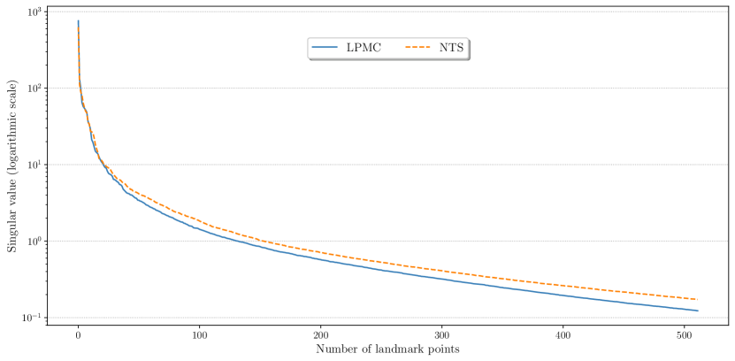
Figure 1: Singular values of the kernel matrix $\mathbf{K}$ for the LPMC and NTS datasets

The results for the LPMC and NTS datasets are illustrated in Figures 2 and 3, respectively. The standard Nyström method using uniform sampling is denoted by the blue line, the Nyström method using the $k$-means sampling strategy is represented by the orange line, the DAC ridge-leverage Nyström by the green line, and the RLS-Nyström by the red line.

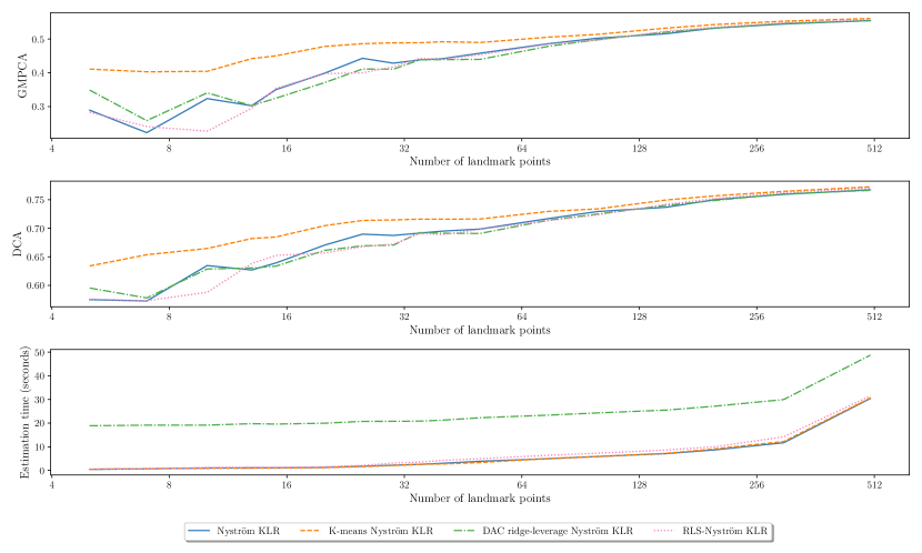
Figure 2: Comparison of Nyström sampling techniques on the LPMC dataset

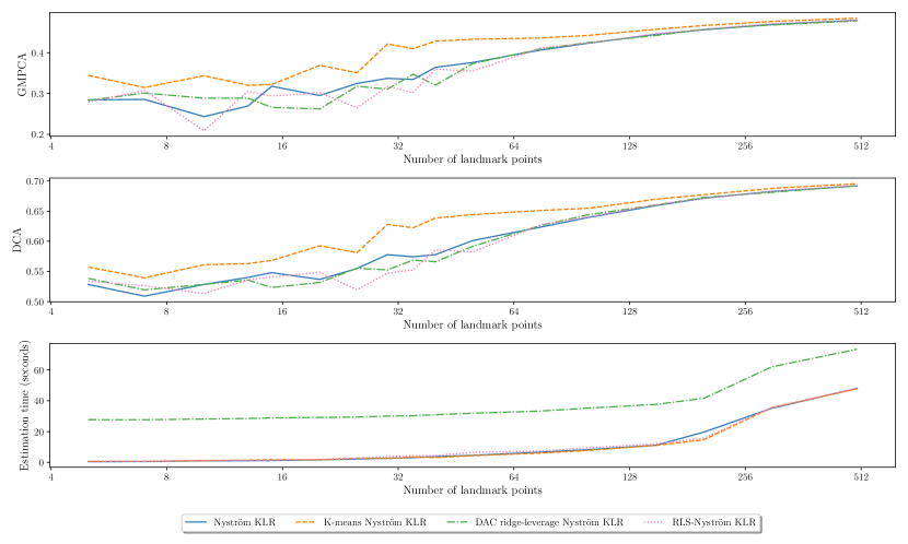
Figure 3: Comparison of Nyström sampling techniques on the NTS dataset

In both datasets, as the number of landmark points in the Nyström method increases, all the methods eventually converge to a similar level of accuracy, equal to the optimal rank $C$ Nyström approximation $\widehat{\mathbf{K}}_{C}$, approaching the performance that would be achieved by directly applying KLR without the Nyström approximation. However, it is important to highlight that using KLR directly, without Nyström, on these datasets would not be feasible due to the size of the kernel matrix. To illustrate this, storing the training matrices ($70\%$ of the observations) of the LPMC and NTS datasets would require approximately $22$ GB and $194$ GB of RAM memory, respectively. Hence, the adoption of the techniques described here becomes indispensable for handling such large datasets.

Regarding computational costs, all methods give similar performance, except for the DAC ridge-leverage Nyström, which requires more time to compute the leverage indices. The RLS-Nyström method also takes slightly longer than the $k$-means Nyström method, although the difference is minimal.

The analysis of the results suggests that the $k$-means Nyström KLR method exhibits faster convergence on both datasets, especially when the number of landmark points is small. This can be evidenced by the lower values of the GMPCA and DCA indices when using less than $100$ landmark points. Additionally, the results of the NTS dataset indicate that, as the dataset size increases, this method becomes more effective when working with few landmark points. However, as the number of landmark points grows larger, there is little discernible difference between the various techniques, except for a slight overall improvement in GMPCA and DCA. Nevertheless, it should be noted that the estimation time of the KLR model and the size of the kernel matrix will significantly increase when using a large number of landmark points.

6.3 Comparison of the Nyström KLR method with other ML algorithms on large datasets

Having studied the behaviour of the different Nyström-based KLR methods, in this experiment, these methods were compared with several state-of-the-art ML methods and a MNL model. The purpose of this comparison was to demonstrate that the Nyström KLR method can serve as a viable alternative to other methods for large datasets. For this experiment, a baseline model was established using a MNL with linear utility functions, which were estimated using Biogeme.

The results of this experiment are set out in Table 1. As seen in Figure 2 for the LPMC dataset, the Nyström KLR with $500$ landmark points returns asymptotic values for the DCA and GMPCA, so there is hardly any difference in performance between the models. Hence, $500$ landmark points were used for the Nyström KLR models. For the NTS dataset, a much larger dataset, Figure 3 shows that for $500$ landmark points the DCA and GMPCA indices still have a small positive slope, therefore $1,000$ landmark points were chosen for the Nyström methods. If the number of landmark points is reduced, it can be seen that the performance of the $k$-means Nyström method would decrease slightly, while the other Nyström methods would experience a more severe decrease.

It is important to note that the estimated size of the training kernel matrices in these models is approximately $0.2$ GB and $1.2$ GB for the LPMC and NTS datasets, respectively. This represents a reduction of $110$ and $160$ times their size, respectively, compared to traditional KLR models, which makes the application of this model feasible for such large datasets.

In terms of the computational time required to estimate the Nyström KLR models, although they are still significant, they are much lower than those of the linear SVM model, especially for very large datasets such as NTS, and similar to those of the SVM with Nÿstrom. Furthermore, the estimation time of all Nyström KLR models, except the DAC ridge-leverage, is lower than the time required by the MNL models, commonly used by practitioners in this field, for such large datasets.

Finally, analysing the performance of the models, it can be observed that the ensemble-based methods (such as XGBoost or RF) and neural networks are the best performers in terms of DCA and GMPCA. The best-performing model with respect to each index in both datasets is marked in bold, which in this case always corresponds to the XGBoost model. This finding is in line with other recent studies in the literature (Wang et al., 2021).

Regarding the KLR models, the best KLR implementation for each dataset is marked with an asterisk ‘*’. It can be observed that for the LPMC dataset, which is the smallest one, the results of all the Nyström KLR models are quite close to those of the top-performing ML algorithms, which suggests they are promising models. However, by employing sampling strategies, the Nystrom-based KLR models demonstrate improved performance compared to the base MNL model. It is noteworthy that, in the NTS dataset, the Nyström KLR methods yield lower scores in terms of DCA. Nevertheless, they still provide better approximations to the probability of each alternative, as measured through the GMPCA, compared to the MNL models.

There are two plausible explanations for the weaker results in the NTS dataset. The first relates to the significant class imbalance observed in the ‘public transport’ and ‘walk’ alternatives. Table 2 reports the precision scores for each alternative in the test set. It is notable that for the minority classes in the LPMC and NTS datasets, precision scores are generally low across all methods. Significantly, KLR, along with MNL, SVM, and XGBoost, achieve the highest precision scores for the smallest class in both datasets. Addressing this class imbalance through techniques such as resampling or using different evaluation metrics tailored for imbalanced datasets might yield improved results. Future research should address this problem.

Another possible explanation for the performance difference is that the LPMC dataset focuses on discrete choice modelling, whereas the NTS dataset is more oriented towards ML applications, and not all variables are equally important. For instance, the NTS dataset contains a significant number of environmental variables, which might have a reduced impact on the classification process. This issue was highlighted in Martín-Baos et al. (2023), where it was calculated the SHAP values for each variable in both datasets, which allowed the variations in variable importance to be analysed. In the LPMC dataset, numerous variables influence the decision maker, while in the NTS dataset, only a few variables, primarily the ‘distance’, have a notable impact. This highlights the sensitivity of the KLR method to non-significant features, suggesting the importance of conducting an attribute analysis prior to applying these techniques. The poor performance of the Nyström SVM on this dataset may also be attributed to these reasons, as well as to the need for a greater number of landmark points for this model.

Table 1: Evaluation of DCA and GMPCA indices in the test set and estimation time by model for LPMC and NTS datasets

	LPMC			NTS
	DCA	GMPCA	Estimation time (s)	DCA	GMPCA	Estimation time (s)
MNL	72.54	48.85	623.43	65.42	43.83	855.61
SVM	73.61	49.92	193.48	63.22	43.34	765.59
LinearSVM	72.13	48.92	691.21	64.64	43.72	3,963.52
RF	73.58	50.14	2.67	68.19	46.84	1.87
XGBoost	74.71	51.85	82.04	68.72	48.05	138.72
NN	73.87	50.72	5.25	68.40	47.12	7.51
Nyström KLR	73.45	50.41*	303.39	64.98	44.53*	776.46
k-means Nyström KLR	73.46	50.35	309.40	65.09*	44.50	719.25
DAC ridge-leverage Nyström KLR	73.49	50.33	507.37	64.91	44.41	1,010.26
RLS-Nyström KLR	73.62*	50.43	324.85	64.81	44.52	727.24

Table 2: Evaluation of precision score for each alternative in the test sets for LPMC and NTS datasets

	LPMC				NTS
	Walk	Bike	Public Transport	Car	Walk	Bike	Public Transport	Car
MNL	0.66	0.50	0.77	0.72	0.56	0.51	0.62	0.72
SVM	0.66	0.38	0.78	0.74	0.55	0.53	0.70	0.66
LinearSVM	0.67	0.00	0.78	0.70	0.54	0.49	0.00	0.71
RF	0.70	0.00	0.75	0.74	0.64	0.54	0.66	0.74
XGBoost	0.71	0.31	0.76	0.75	0.63	0.54	0.65	0.75
NN	0.70	0.00	0.76	0.74	0.60	0.54	0.62	0.75
Nyström KLR	0.67	0.23	0.76	0.74	0.60	0.51	0.71	0.70
K-means Nyström KLR	0.67	0.27	0.76	0.74	0.61	0.51	0.71	0.70
DAC ridge-leverage Nyström KLR	0.67	0.24	0.76	0.74	0.61	0.51	0.73	0.70
RLS-Nyström KLR	0.67	0.18	0.76	0.74	0.61	0.51	0.73	0.70

6.4 Comparative of optimisation techniques for Nyström KLR

After overcoming the challenge of storing large kernel matrices, the subsequent step involves determining the most efficient optimisation algorithm to estimate the vector of parameters in KLR. The estimation process involves solving the optimisation problem in Equation (7), where the loss function is the negative conditional log-likelihood, leading to a procedure called minimising RNLL or, equivalently, maximising PMLE. Typically, the algorithms used for solving this PMLE problem rely on the gradient of the objective function.

From a theoretical perspective, training MNL or KLR models using PMLE is equivalent, as both require estimating functions that are linear in their parameters. However, the differences appear from a computational point of view due to the number of parameters in the models. In the case of MNL (in the context of RUM), the number of parameters increases on the order of ${\cal O}(M\cdot I)$, where $M$ is the dimension of the original input space, i.e., $\mathbf{X}\subset\mathbb{R}^{M}$, and $I$ is the number of alternatives in the choice set. On the other hand, KLR grows more abruptly with ${\cal O}(N\cdot I)$, where $N$ is the number of observations. Consequently, training KLR models poses a computational challenge, as it requires the estimation of a large number of coefficients.

As discussed earlier, the Nyström KLR model has the advantage of reducing the size of the kernel matrix, which makes the number of parameters to be estimated in the model increase on the order of ${\cal O}(C\cdot I)$, where $C$ is the number of landmark points. This advantageous feature allows the number of required parameters to no longer depend on the size of the dataset but only on the number of landmark points, which is a significant advantage for large datasets. Thus, the number of parameters becomes more similar to that of the MNL, making the Nyström approach a promising method for scalable estimation on large datasets.

To compare the different optimisation techniques, it was necessary to first implement these optimisation methods within the GKLR Python package. The experimental setup and datasets of the previous section are maintained, and it was selected a $k$-means Nyström KLR method for this comparison. Specifically, the LPMC dataset was used, with $500$ landmark points, while the NTS dataset employed $1,000$ landmark points.

The $k$-means Nyström KLR model was estimated for both datasets with a PMLE and using the L-BFGS-B, GD, Momentum, and Adam optimisation methods. For the L-BFGS-B method, convergence was ensured by setting a tolerance of $10^{-12}$ and a maximum of $10,000$ iterations. This guarantees that the method terminates only when it can no longer explore lower values of the objective function. Regarding the GD, Momentum, and Adam methods, they were set to undergo a total of $5,000$ iterations (epochs) with a time-based learning rate decay strategy. Furthermore, a hyperparameter tuning process was conducted for the learning rate and decay rate through grid search within a predefined search space for all optimisation methods.

Figure 4 illustrates the relationship between the objective function value and the required estimation time for each optimisation method using the LPMC dataset. A similar representation is offered in Figure 5 for the NTS dataset, which is notably larger in scale. Furthermore, Table 3 provides a comprehensive overview of the final optimisation results for each method.

Upon analysis, it becomes evident that the L-BFGS-B method is the optimal choice for training the $k$-means Nyström KLR model under the PMLE framework. Closely behind are the Adam and Momentum methods, in that order. Notably, the GD method lags behind the other algorithms even with adjustments to the learning rate or increased computational time. Additional numerical tests, which have not been reported, indicate that the Adam method can achieve the best results when a sufficient number of iterations are performed with a good hyperparameter set. However, it is essential to note that the Adam method takes approximately $4$ to $6$ times longer (in terms of CPU time) than the L-BFGS-B method to achieve and surpass these optimal values.

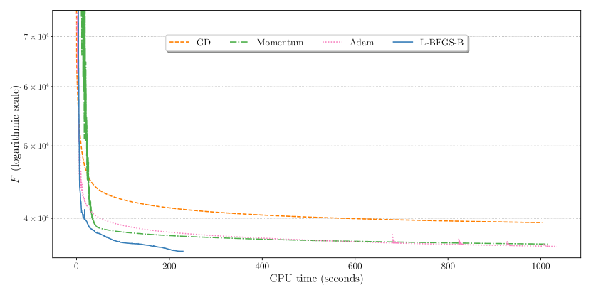
Figure 4: Comparison of optimisation algorithms for KLR on the LPMC dataset

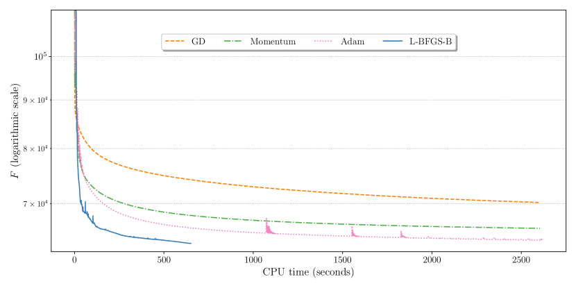
Figure 5: Comparison of optimisation algorithms for KLR on the NTS dataset

Table 3: Optimisation results

	LPMC		NTS
	Final Loss	CPU Time (s)	Final Loss	CPU Time (s)
L-BFGS-B	36,144.43	229.31	63,552.09	650.78
GD	39,473.54	1,003.81	70,173.70	2,599.00
Momentum	36,949.68	1,020.09	65,908.53	2,605.57
Adam	36,686.48	1,035.54	64,020.47	2,620.94

An important consideration of this study is that to obtain the graphs presented, it was necessary to report the value of the objective function at every iteration of the estimation methods. However, obtaining the value of the objective function using the KLR method with large datasets is computationally expensive. Consequently, all estimation methods display CPU times that surpass those that would have been the case if the objective function’s value were not reported, or if it were computed only at intervals of $\Delta_{t}$ iterations.

7 Conclusion and future work

This study has addressed the challenges of applying the KLR technique to discrete choice modelling with large datasets. Despite inherent complexities posed by memory demands and the large number of parameters in these models, the proposed solution effectively addressed scalability obstacles. The contributions of this research can be summarised into four key points.

Firstly, a theoretical study was conducted to characterise the solution set of the KLR training problem, identifying that the common practice in the literature of constraining the parameters of the last alternative to zero is suboptimal with respect to the so-called restricted training problem. Furthermore, the performance of KLR with the Nyström approximation was rigorously analysed, characterising the solution of Nyström KLR, and establishing the first error bound.

Secondly, the study assessed the feasibility of using the Nyström approach within KLR to analyse large datasets. This technique significantly reduced kernel matrix size, while upholding the performance of the model. In the datasets used for this comparison, performance superior to that of traditional discrete choice models was achieved, such as MNL, while reducing the size of the kernel matrices by a factor of between $110$ and $160$, compared to the original KLR model. A comprehensive comparison of four Nyström methods demonstrated their potential for efficiently handling datasets exceeding $200,000$ observations. These four methods encompass distinct sampling approaches, including a uniform, $k$-means, and two non-uniform strategies based on leverage scores. They were tested on a multi-categorical classification problem within the domain of transport mode choice, using large datasets. The $k$-means Nyström strategy emerged as particularly effective, particularly when a modest number of landmark points is used to approximate the kernel matrix. However, it was found that when the number of landmark points increases, all strategies converge to the optimal rank-$C$ approximation of Nyström.

Thirdly, the performance of Nyström-based strategies was benchmarked against traditional methods commonly applied in the transport field, such as MNL and state-of-the-art ML techniques. The results concluded that while effective, the Nyström KLR models did not surpass the superior performance of methods like XGBoost. However, a noteworthy observation is that top-performing methods like ensemble approaches (XGBoost or RF) often struggle in estimating the derivatives of probabilities, as reported by Martín-Baos et al. (2023), which is crucial for extracting econometric indicators. The KLR approach allows the derivatives of the probabilities to be estimated accurately (Martín-Baos et al., 2020), and this is what motivates further research in the direction of obtaining econometric information using these models.

Fourthly, it was found that the results of the Nyström KLR model depend to a large extent on the correct estimation of their parameters and hyperparameters. Therefore, this research looks at a number of optimisation techniques for Nyström KLR model estimation and finds that the L-BFGS-B method emerges as the most effective choice, closely followed by the Adam method (which is a commonly-used technique for training Deep Neural Networks (DNNs)).

Promising avenues for further work include exploring the capabilities of the mini-batch SGD for the estimation of the Nyström KLR model. This method offers significant advantages, including accelerated convergence and enhanced generalisation performance, as evidenced in the existing literature (Bottou et al., 2018). However, integrating mini-batch SGD into the current GKLR package (https://github.com/JoseAngelMartinB/gklr) proves challenging for large datasets as the gradient computation requires calculating the Kronecker product for a subset of the kernel matrix (i.e., the mini-batch). In the current implementation of the package, this operation dominates the computational cost. Consequently, employing mini-batches entails multiple iterations of the Kronecker product, thereby escalating computational demands proportionally. Addressing this limitation requires optimising the estimation module of the GKLR package to take advantage of the parallel processing capabilities of the CPU to overcome this barrier.

Lastly, datasets applied in discrete choice modelling, such as survey datasets, might exhibit imbalances due to unequal representation of alternatives in the population. The study shows that the ML methods achieve lower precision scores on the less represented classes. Addressing these imbalances is another avenue for future research. Exploring data balancing techniques and investigating their impact on model performance holds promise for further refinement. In essence, this study contributes valuable insights into the effectiveness and limitations of Nyström KLR in handling large datasets, paving the way for continued advancements in the field.

Declaration of Generative AI and AI-assisted technologies in the writing process

During the preparation of this work, the authors used OpenAI GPT-3.5 and Grammarly to aid in generating and refining natural language text for different sections of the manuscript. After using this tool, the authors reviewed and edited the content as needed and take full responsibility for the content of the publication.

Acronyms

CEL

Cross-Entropy Loss

DCA

Discrete Classification Accuracy

DCM

Discrete Choice Models

DNN

Deep Neural Network

GD

Gradient Descent

GMPCA

Geometric Mean Probability of Correct Assignment

GP

Gaussian Process

KLR

Kernel Logistic Regression

ML

Machine Learning

MLE

Maximum Likelihood Estimation

MLP

Multilayer Perceptron

MNL

Multinomial Logit

NL

Nested Logit Model

NN

Neural Network

PMLE

Penalised Maximum Likelihood Estimation

RF

Random Forests

RKHS

Reproducing Kernel Hilbert Spaces

RNLL

Regularised Negative Log-Likelihood

RUM

Random Utility Model

SGD

Stochastic Gradient Descent

SVD

Singular Value Decomposition

SVM

Support Vector Machine

WTP

Willingness to Pay

XGBoost

Extreme Gradient Boosting

Appendix A Analysis of the KLR model overspecification under RNLL

This appendix is intended to show the sources of overspecification of RNLL.

Lemma A.1

The function $\mathbf{h}_{\cdot i}(\boldsymbol{\upsilon}_{\cdot\cdot})=\mathbf{p}_{\cdot i}(\boldsymbol{\alpha}_{\cdot\cdot}+\boldsymbol{\upsilon}_{\cdot\cdot})$ remains constant over the vector space $\boldsymbol{\upsilon}_{\cdot\cdot}\in V+L(\mathbf{K})^{\perp}$ where:

$$V=\left\{\mathbf{1}^{\top}\otimes\boldsymbol{\beta}:\boldsymbol{\beta}\in\mathbb{R}^{N\times 1}\right\}$$

Proof.
Let $\boldsymbol{\alpha}_{\cdot\cdot}\in\mathbb{R}^{N\times I}$ and $\boldsymbol{\alpha}^{*}_{\cdot\cdot}=\boldsymbol{\alpha}_{\cdot\cdot}+\mathbf{1}^{\top}\otimes\boldsymbol{\beta}+\boldsymbol{\alpha}^{\perp}_{\cdot\cdot}$ where $\boldsymbol{\alpha}^{\perp}_{\cdot\cdot}\in L(\mathbf{K})^{\perp}$, then,

$$p_{ni}\left(\boldsymbol{\alpha}^{*}_{\cdot\cdot}\right) =\frac{\exp\left(\mathbf{k}_{n}^{\top}(\boldsymbol{\alpha}_{\cdot i}+\boldsymbol{\beta}+\boldsymbol{\alpha}^{\perp}_{\cdot i})\right)}{\sum_{j=1}^{I}\exp\left(\mathbf{k}_{n}^{\top}(\boldsymbol{\alpha}_{\cdot j}+\boldsymbol{\beta}+\boldsymbol{\alpha}^{\perp}_{\cdot j})\right)}=\frac{\exp\left(\mathbf{k}_{n}^{\top}\boldsymbol{\alpha}_{\cdot i}\right)\exp\left(\mathbf{k}_{n}^{\top}\boldsymbol{\beta}\right)\exp(0)}{\sum_{j=1}^{I}\exp\left(\mathbf{k}_{n}^{\top}\boldsymbol{\alpha}_{\cdot j}\right)\exp\left(\mathbf{k}_{n}^{\top}\boldsymbol{\beta}\right)\exp(0)}$$

$$=\frac{\exp\left(\mathbf{k}_{n}^{\top}\boldsymbol{\alpha}_{\cdot i}\right)}{\sum_{j=1}^{I}\exp\left(\mathbf{k}_{n}^{\top}\boldsymbol{\alpha}_{\cdot j}\right)}=p_{ni}\left(\boldsymbol{\alpha}_{\cdot\cdot}\right)$$ (38)

_■

Remark A.1

Applying the MLE method to KLR (by setting $\lambda=0$), it will not be possible to univocally determine the function $f_{i}(\mathbf{x})$, since there are infinite functions $f^{*}_{i}(\mathbf{x})$ leading to the same probability functions $\mathbf{p}_{\cdot i}(\boldsymbol{\alpha}_{\cdot\cdot})$ and, therefore, the log-likelihood value remains constant. This leads to the overspecification of the MLE problem, resulting in an infinite number of optimal solutions. To address this, a potential solution involves setting the parameter value for the last alternative, $I$, to $\mathbf{0}$. This choice is equivalent to setting $\boldsymbol{\beta}=-\boldsymbol{\alpha}_{I}$ yields another optimal MLE solution, where the parameter vector of the last alternative is $\mathbf{0}$. This restriction does not compromise the quality of the solution of the training problem, but the analysis is not correct when $\lambda>0$.

The proof to Theorem 3.1 is given as follows.

Proof.
Let $\boldsymbol{\alpha}^{*}_{\cdot\cdot}$ be a solution to the training problem specified in Equation (7). Then, this solution can be written as:

$$\boldsymbol{\alpha}^{*}_{\cdot\cdot}={\mathcal{P}}^{\perp}_{L(\mathbf{K})}\left(\boldsymbol{\alpha}^{*}_{\cdot\cdot}\right)+{\mathcal{P}}^{\perp}_{L(\mathbf{K})^{\perp}}\left(\boldsymbol{\alpha}^{*}_{\cdot\cdot}\right)=\boldsymbol{\aleph}^{*}_{\cdot\cdot}+\boldsymbol{\eta}_{\cdot\cdot}$$ (39)

As $\boldsymbol{\eta}_{\cdot\cdot}=(\mathbf{1}^{\top}\otimes\mathbf{0})+\boldsymbol{\eta}_{\cdot\cdot}\in V+L(\mathbf{K})^{\perp}$, applying the Lemma A.1 gives:

$$\mathbf{p}_{\cdot i}\left(\boldsymbol{\alpha}^{*}_{\cdot\cdot}\right)=\mathbf{p}_{\cdot i}\left(\boldsymbol{\aleph}^{*}_{\cdot\cdot}\right)$$ (40)

On the other hand, since $\boldsymbol{\eta}_{\cdot\cdot}\in L(\mathbf{K})^{\perp}$:

$$\mathbf{K}\,\boldsymbol{\eta}_{\cdot\cdot}=\mathbf{0}\Rightarrow\mathbf{K}\,\boldsymbol{\alpha}^{*}_{\cdot\cdot}=\mathbf{K}\,\boldsymbol{\aleph}^{*}_{\cdot\cdot}$$ (41)

which ensures that the regularisation term satisfies:

$$\frac{\lambda}{2}\sum_{i=1}^{I}\boldsymbol{\alpha}_{\cdot i}^{\top}\mathbf{K}\boldsymbol{\alpha}_{\cdot i}=\frac{\lambda}{2}\sum_{i=1}^{I}\boldsymbol{\aleph}_{\cdot i}^{\top}\mathbf{K}\boldsymbol{\aleph}_{\cdot i}$$ (42)

From Equations (40) and (42) it can be obtained that:

$$\mathcal{L}(\boldsymbol{\alpha}^{*}_{\cdot\cdot})=\mathcal{L}(\boldsymbol{\aleph}^{*}_{\cdot\cdot})$$ (43)

Furthermore, Equation (43) guarantees that $\boldsymbol{\aleph}^{*}_{\cdot\cdot}$ is a minimiser of:

$$\min_{\boldsymbol{\alpha}_{\cdot\cdot}\in\mathbb{R}^{N\times I}}\mathcal{L}(\boldsymbol{\alpha}_{\cdot\cdot})$$ (44)

Because $\mathbb{R}^{N\times 1}=$$L(\mathbf{K})\oplus L(\mathbf{K})^{\perp}$, it holds that:

$$\min_{\boldsymbol{\alpha}_{\cdot\cdot}\in L(\mathbf{K})}\mathcal{L}(\boldsymbol{\alpha}_{\cdot\cdot})\geq\min_{\boldsymbol{\alpha}_{\cdot\cdot}\in\mathbb{R}^{N\times I}}\mathcal{L}(\boldsymbol{\alpha}_{\cdot\cdot})$$ (45)

From the fact that $\boldsymbol{\aleph}^{*}_{\cdot\cdot}\in L(\mathbf{K})$, and from the optimality of $\boldsymbol{\aleph}^{*}_{\cdot\cdot}$ for the problem (44), Equation (45) leads to the optimality of $\boldsymbol{\aleph}^{*}_{\cdot\cdot}$ for the restricted problem $\min_{\boldsymbol{\alpha}_{\cdot\cdot}\in L(\mathbf{K})}\mathcal{L}(\boldsymbol{\alpha}_{\cdot\cdot}).$

To prove that the restricted problem has a unique solution, consider the decomposition of SVD of the kernel matrix:

$$\mathbf{K}=\mathbf{U}\boldsymbol{\Sigma}\mathbf{U}^{\top}$$

where $\mathbf{U},\boldsymbol{\Sigma}$ are an $N\times R$ column-orthogonal matrix and an $R\times R$ diagonal matrix with nonnegative entries, respectively. Assuming that $\hbox{rank}(\mathbf{K})=R$ then $\mathbf{K}$ has $\sigma_{1}>\cdots>\sigma_{R}>0$ eigenvalues and $\boldsymbol{\Sigma}=\hbox{diag}(\sigma_{1}\cdots\sigma_{R})$.

As the column vectors of $\mathbf{U}$ form a basis of the vector space $L(\mathbf{K})$:

$$\boldsymbol{\alpha}_{\cdot\cdot}\in L(\mathbf{K})\Leftrightarrow\boldsymbol{\alpha}_{\cdot\cdot}=\mathbf{U}\boldsymbol{\Sigma}^{-\frac{1}{2}}\boldsymbol{\beta}_{\cdot\cdot}$$ (46)

where $\boldsymbol{\Sigma}^{-\frac{1}{2}}=\hbox{diag}(\sigma^{-1/2}_{1}\cdots\sigma^{-1/2}_{R})$ and $\boldsymbol{\beta}_{\cdot\cdot}\in\mathbb{R}^{R\times I}$.

Now, the restricted training problem is expressed in terms of the new variable $\boldsymbol{\beta}_{\cdot\cdot}$ as:

$$\boldsymbol{\alpha}^{\top}_{\cdot i}\mathbf{K}\boldsymbol{\alpha}_{\cdot i}=\boldsymbol{\beta}^{\top}_{\cdot i}\boldsymbol{\Sigma}^{-\frac{1}{2}}\mathbf{U}^{\top}\mathbf{K}\mathbf{U}\boldsymbol{\Sigma}^{-\frac{1}{2}}\boldsymbol{\beta}_{\cdot i}=\boldsymbol{\beta}^{\top}_{\cdot i}\boldsymbol{\Sigma}^{-\frac{1}{2}}\mathbf{U}^{\top}\mathbf{U}\boldsymbol{\Sigma}\mathbf{U}^{\top}\mathbf{U}\boldsymbol{\Sigma}^{-\frac{1}{2}}\boldsymbol{\beta}_{\cdot i}=\boldsymbol{\beta}^{\top}_{\cdot i}\mathbb{I}_{R}\boldsymbol{\beta}_{\cdot i}$$ (47)

where $\mathbb{I}_{R}$ is the identity matrix of order $R$. As the identity matrix is positive definite this shows that the penalisation term for the restricted training problem is a strictly convex function.

On the other hand, the latent functions can be written as:

$$\mathbf{f}_{\cdot\cdot}=\mathbf{K}\boldsymbol{\alpha}_{\cdot\cdot}=\mathbf{K}\mathbf{U}\boldsymbol{\Sigma}^{-\frac{1}{2}}\boldsymbol{\beta}_{\cdot\cdot}=\mathbf{U}\boldsymbol{\Sigma}\mathbf{U}^{\top}\mathbf{U}\boldsymbol{\Sigma}^{-\frac{1}{2}}\boldsymbol{\beta}_{\cdot\cdot}=\mathbf{U}\boldsymbol{\Sigma}^{\frac{1}{2}}\boldsymbol{\beta}_{\cdot\cdot}$$ (48)

Letting $\mathbf{B}=\mathbf{U}\boldsymbol{\Sigma}^{\frac{1}{2}}\in\mathbb{R}^{N\times I}$ gives:

$$p_{ni}(\boldsymbol{\alpha}_{\cdot\cdot})=\frac{\exp(\mathbf{B}_{n\cdot}\boldsymbol{\beta}_{\cdot i})}{\sum_{j=1}^{I}\exp(\mathbf{B}_{n\cdot}\boldsymbol{\beta}_{\cdot j})}=p_{ni}(\boldsymbol{\beta}_{\cdot\cdot})$$ (49)

$${\mathcal{L}}(\boldsymbol{\beta}_{\cdot\cdot})=-\frac{1}{N}\sum_{n=1}^{N}\sum_{i=1}^{I}y_{ni}\log p_{ni}(\boldsymbol{\beta}_{\cdot\cdot})+\frac{\lambda}{2}\sum_{i=1}^{I}\boldsymbol{\beta}_{\cdot i}^{\top}\mathbb{I}_{R}\boldsymbol{\beta}_{\cdot i},$$ (50)

If $\lambda>0$, it is observed that the objective function of the restricted training problem ${\mathcal{L}}(\boldsymbol{\beta}_{\cdot\cdot})$ can be seen as the sum of two main components: (i) the negative log-likelihood and (ii) a penalty term. Notably, Daganzo and Kusnic (1993) and Hasan et al. (2016) demonstrated the convexity of component (i) within the broader context of the Nested Logit Model (NL) model, which encompasses MNL. Furthermore, the term (ii) also exhibits strictly convex characteristics due to the positive definiteness inherent in the identity matrix $\mathbb{I}_{R}$ and ${\mathcal{L}}(\boldsymbol{\beta}_{\cdot\cdot})$ becomes a strictly convex function. As a result, the restricted training problem has a unique solution. Since it has been proved that $\boldsymbol{\aleph}^{*}_{\cdot\cdot}$ is a minimiser of the restricted training problem, this is the only solution of the problem.
_■

Appendix B Error bounds for Nyström KLR

Lemma B.1

Let $\mathbf{p}_{\cdot i}(\boldsymbol{\alpha}_{\cdot\cdot})$ be the probabilities vector computed for the kernel matrix $\mathbf{K}$, and let $\widehat{\mathbf{p}}_{\cdot i}(\boldsymbol{\alpha}_{\cdot\cdot})$ be the same probabilities vector found by using the approximation $\widehat{\mathbf{K}}$. Then:

$$\widehat{\mathbf{p}}_{\cdot i}(\boldsymbol{\alpha}_{\cdot\cdot})=\mathbf{p}_{\cdot i}(\boldsymbol{\alpha}_{\cdot\cdot})-\mathbf{p}_{\cdot\cdot}(\boldsymbol{\alpha}_{\cdot\cdot})\left[\boldsymbol{\alpha}_{\cdot\cdot}^{\top}(\widehat{\mathbf{K}}-\mathbf{K})\right]\mathbf{p}_{\cdot i}(\boldsymbol{\alpha}_{\cdot\cdot})+\boldsymbol{\varepsilon}$$ (51)

where $\|\boldsymbol{\varepsilon}\|_{2}=o(\|(\widehat{\mathbf{K}}-\mathbf{K})^{\top}\boldsymbol{\alpha}_{\cdot\cdot}\|_{2,\infty})$.

Proof.
Consider the softmax function:

$$S_{i}(\mathbf{f})=\dfrac{\exp(\mathbf{f}_{i})}{\sum_{j=1}^{I}\exp(\mathbf{f}_{j})}$$ (52)

This function is expressed by its first-order Taylor polynomial expanded at $\mathbf{f}$:

$$S_{i}(\widehat{\mathbf{f}})=S_{i}(\mathbf{f})-S_{i}(\mathbf{f})\sum_{j=1}^{I}S_{j}(\mathbf{f})\left[\widehat{\mathbf{f}}_{j}-\mathbf{f}_{j}\right]+o(\|\widehat{\mathbf{f}}-\mathbf{f}\|_{2})$$ (53)

Letting $\widehat{\mathbf{f}}_{nj}=\widehat{\mathbf{k}}_{n}^{\top}\boldsymbol{\alpha}_{\cdot j}$ and $\mathbf{f}_{nj}=\mathbf{k}_{n}^{\top}\boldsymbol{\alpha}_{\cdot j}$, then $\widehat{\mathbf{f}}_{n\cdot}=\widehat{\mathbf{k}}_{n}^{\top}\boldsymbol{\alpha}_{\cdot\cdot}$ and $\mathbf{f}_{n\cdot}=\mathbf{k}_{n}^{\top}\boldsymbol{\alpha}_{\cdot\cdot}$.

The probability that user $n$ selects alternative $i$, computed either exactly or approximately using the feature vector, is given respectively by:

$$p_{ni}=S_{i}(\mathbf{f}_{n\cdot})=S_{i}(\mathbf{k}_{n}^{\top}\boldsymbol{\alpha}_{\cdot\cdot})$$

$$\widehat{p}_{ni}=S_{i}(\widehat{\mathbf{f}}_{n\cdot})=S_{i}(\widehat{\mathbf{k}}_{n}^{\top}\boldsymbol{\alpha}_{\cdot\cdot})$$

Applying Taylor’s expansion to Equation (53) gives:

$$\widehat{p}_{ni}=p_{ni}-p_{ni}\sum_{j=1}^{I}p_{nj}[\widehat{\mathbf{k}}_{n}^{\top}\boldsymbol{\alpha}_{\cdot j}-\mathbf{k}_{n}^{\top}\boldsymbol{\alpha}_{\cdot j}]+o(\|(\widehat{\mathbf{k}}_{n}-\mathbf{k}_{n})^{\top}\boldsymbol{\alpha}_{\cdot\cdot}\|_{2})$$ (54)

Rewriting Equation (54) using matrices:

$$\widehat{p}_{ni}=p_{ni}-p_{ni}\,\mathbf{p}_{n\cdot}\left[\boldsymbol{\alpha}_{\cdot\cdot}^{\top}(\widehat{\mathbf{k}}_{n}-\mathbf{k}_{n})\right]+o(\|(\widehat{\mathbf{k}}_{n}-\mathbf{k}_{n})^{\top}\boldsymbol{\alpha}_{\cdot\cdot}\|_{2})$$ (55)

Then, expanding the above expression with respect to $n$:

$$\widehat{\mathbf{p}}_{\cdot i}=\mathbf{p}_{\cdot i}-\mathbf{p}_{\cdot\cdot}\left[\boldsymbol{\alpha}_{\cdot\cdot}^{\top}(\widehat{\mathbf{K}}-\mathbf{K})\right]\mathbf{p}_{\cdot i}+\boldsymbol{\varepsilon}$$ (56)

where for the error vector $\boldsymbol{\varepsilon}$, all components satisfy $\boldsymbol{\varepsilon}_{n}=o(\|(\widehat{\mathbf{k}}_{n}-\mathbf{k}_{n})^{\top}\boldsymbol{\alpha}_{\cdot\cdot}\|_{2})$, therefore $\boldsymbol{\varepsilon}_{n}=o\left(\underset{n}{\max}{\|(\widehat{\mathbf{k}}_{n}-\mathbf{k}_{n})^{\top}\boldsymbol{\alpha}_{\cdot\cdot}}\|_{2}\right)=o(\|(\widehat{\mathbf{K}}-\mathbf{K})^{\top}\boldsymbol{\alpha}_{\cdot\cdot}\|_{2,\infty})$, and it follows that $\|\boldsymbol{\varepsilon}\|_{2}=o(\|(\widehat{\mathbf{K}}-\mathbf{K})^{\top}\boldsymbol{\alpha}_{\cdot\cdot}\|_{2,\infty})$.
_■

The proof of Theorem 4.1 is given as follows.

Proof.
By hypothesis, $\widehat{\mathbf{K}}$ is a Nyström approximation associated to the sketching matrix $\mathbf{P}$, giving $\mathbf{C}=\mathbf{K}\mathbf{P}.$ It holds that $L(\mathbf{C})=L(\widehat{\mathbf{K}})$ and so, this linear space can be interchangeably referred to in the proof.

Let $\boldsymbol{\aleph}^{*}_{\cdot\cdot}$ be a solution, Equation (7). It then satisfies the optimality conditions:

$$\mathbf{K}\underset{\mathbf{z}_{i}}{\underbrace{\left[N\lambda\boldsymbol{\aleph}^{*}_{\cdot i}-\mathbf{p}_{\cdot i}(\boldsymbol{\aleph}^{*}_{\cdot\cdot})+\boldsymbol{y}_{\cdot i}\right]}}=\mathbf{0},\hskip 28.45274pti=1,\cdots,I.$$ (57)

Equation (57) shows that $\mathbf{K}\mathbf{z}_{i}=\mathbf{0}\Rightarrow\mathbf{z}_{i}\in L(\mathbf{K})^{\perp}$. Moreover, by hypothesis, $\widehat{\mathbf{K}}$ is a Nyström approximation and, therefore, $L(\widehat{\mathbf{K}})\subseteq L(\mathbf{K})$ from which it follows that $L(\mathbf{K})^{\perp}\subseteq L(\widehat{\mathbf{K}})^{\perp}$ and therefore $\mathbf{z}_{i}\in L(\widehat{\mathbf{K}})^{\perp}$. This leads to $\widehat{\mathbf{K}}\mathbf{z}_{i}=\mathbf{0}$, that is:

$$\widehat{\mathbf{K}}\left[N\lambda\boldsymbol{\aleph}^{*}_{\cdot i}-\mathbf{p}_{\cdot i}(\boldsymbol{\aleph}^{*}_{\cdot\cdot})+\boldsymbol{y}_{\cdot i}\right]=\mathbf{0},\hskip 28.45274pti=1,\cdots,I.$$ (58)

This solution is uniquely expressed as:

$$\boldsymbol{\aleph}^{*}_{\cdot i}={\mathcal{P}}^{\perp}_{L(\widehat{\mathbf{K}})}(\boldsymbol{\aleph}^{*}_{\cdot i})+{\mathcal{P}}^{\perp}_{L(\widehat{\mathbf{K}})^{\perp}}(\boldsymbol{\aleph}^{*}_{\cdot i})$$ (59)

Letting ${\widehat{\boldsymbol{\chi}}^{*}_{\cdot i}}={\mathcal{P}}^{\perp}_{L(\widehat{\mathbf{K}})}(\boldsymbol{\aleph}^{*}_{\cdot i})$ and ${\widehat{\boldsymbol{\chi}}^{*\perp}_{\cdot i}}={\mathcal{P}}^{\perp}_{L(\widehat{\mathbf{K}})^{\perp}}(\boldsymbol{\aleph}^{*}_{\cdot i})$. Now establish:

$$\widehat{\boldsymbol{\chi}}^{*\top}_{\cdot\cdot}[\mathbf{K}-\widehat{\mathbf{K}}]=\mathbf{0}$$ (60)

The following relationship (refer to Equation (18) for its derivation)

$$\mathbf{K}-\widehat{\mathbf{K}}=\mathbf{K}^{1/2}\left[\mathbb{I}-\boldsymbol{\Pi}^{\perp}_{L(\mathbf{K}^{1/2}\mathbf{P})}\right]\mathbf{K}^{1/2}$$ (61)

allows Equation (60) to be written as:

$$\widehat{\boldsymbol{\chi}}^{*\top}_{\cdot\cdot}[\mathbf{K}-\widehat{\mathbf{K}}]=\widehat{\boldsymbol{\chi}}^{*\top}_{\cdot\cdot}\mathbf{K}^{1/2}\mathbf{A}$$ (62)

where $\mathbf{A}=\left[\mathbb{I}-\boldsymbol{\Pi}^{\perp}_{L(\mathbf{K}^{1/2}\mathbf{P})}\right]\mathbf{K}^{1/2}\subseteq L(\mathbf{K}^{1/2}\mathbf{P})^{\perp}$. On the other hand, $\mathbf{K}^{1/2}=\mathcal{P}^{\perp}_{L(\mathbf{K}^{1/2}\mathbf{P})}(\mathbf{K}^{1/2})+\mathcal{P}^{\perp}_{L(\mathbf{K}^{1/2}\mathbf{P})^{\perp}}(\mathbf{K}^{1/2})$, and so rewriting:

$$\widehat{\boldsymbol{\chi}}^{*\top}_{\cdot\cdot}[\mathbf{K}-\widehat{\mathbf{K}}]=\widehat{\boldsymbol{\chi}}^{*\top}_{\cdot\cdot}\left[\mathcal{P}^{\perp}_{L(\mathbf{K}^{1/2}\mathbf{P})}(\mathbf{K}^{1/2})+\mathcal{P}^{\perp}_{L(\mathbf{K}^{1/2}\mathbf{P})^{\perp}}(\mathbf{K}^{1/2})\right]\mathbf{A}=$$

$$\widehat{\boldsymbol{\chi}}^{*\top}_{\cdot\cdot}\underset{\mathbf{=0(*)}}{\underbrace{\mathcal{P}_{L(\mathbf{K}^{1/2}\mathbf{P})}(\mathbf{K}^{1/2})\mathbf{A}}}+\underset{\mathbf{=0(**)}}{\underbrace{\widehat{\boldsymbol{\chi}}^{*\top}_{\cdot\cdot}\mathcal{P}_{L(\mathbf{K}^{1/2}\mathbf{P})^{\perp}}(\mathbf{K}^{1/2})}}\mathbf{A}=\mathbf{0}$$

The relationship (*) is satisfied by the definition of $\mathbf{A}$. Now consider the relationship $(**)$. Given $\widehat{\boldsymbol{\chi}}^{*}_{\cdot\cdot}\in L(\mathbf{KP})\Rightarrow\widehat{\boldsymbol{\chi}}^{*}_{\cdot\cdot}=\mathbf{KPD}$ with $\mathbf{D}\in\mathbb{R}^{C\times I}$, then:

$$\widehat{\boldsymbol{\chi}}^{*\top}_{\cdot\cdot}=\mathbf{D}^{\top}\mathbf{P}^{\top}\mathbf{K}=\mathbf{D}^{\top}\mathbf{P}^{\top}\mathbf{K}^{1/2}\mathbf{K}^{1/2}=\mathbf{D}^{\top}\mathbf{P}^{\top}\mathbf{K}^{1/2}\left[\mathcal{P}^{\perp}_{L(\mathbf{K}^{1/2}\mathbf{P})}(\mathbf{K}^{1/2})+\mathcal{P}^{\perp}_{L(\mathbf{K}^{1/2}\mathbf{P})^{\perp}}(\mathbf{K}^{1/2})\right]$$ (63)

from which is obtained:

$$\widehat{\boldsymbol{\chi}}^{*\top}_{\cdot\cdot}\mathcal{P}_{L(\mathbf{K}^{1/2}\mathbf{P})^{\perp}}(\mathbf{K}^{1/2}) =\mathbf{D}^{\top}\mathbf{P}^{\top}\mathbf{K}^{1/2}\left[\mathcal{P}^{\perp}_{L(\mathbf{K}^{1/2}\mathbf{P})}(\mathbf{K}^{1/2})+\mathcal{P}^{\perp}_{L(\mathbf{K}^{1/2}\mathbf{P})^{\perp}}(\mathbf{K}^{1/2})\right]\mathcal{P}^{\perp}_{L(\mathbf{K}^{1/2}\mathbf{P})^{\perp}}(\mathbf{K}^{1/2})$$ (64)

$$=\mathbf{D}^{\top}\mathbf{P}^{\top}\mathbf{K}^{1/2}\left[\mathcal{P}^{\perp}_{L(\mathbf{K}^{1/2}\mathbf{P})^{\perp}}(\mathbf{K}^{1/2})\right]^{2}=\mathbf{0}$$ (65)

Using the Taylor expansion at $\boldsymbol{\aleph}^{*}_{\cdot\cdot}$, as given in Lemma B.1:

$$\widehat{\mathbf{p}}_{\cdot i}\left({\widehat{\boldsymbol{\chi}}^{*}_{\cdot\cdot}}\right)=\mathbf{p}_{\cdot i}\left(\boldsymbol{\aleph}^{*}_{\cdot\cdot}\right)-\mathbf{p}_{\cdot\cdot}\left(\boldsymbol{\aleph}^{*}_{\cdot\cdot}\right)\underset{\mathbf{=0}}{\underbrace{\left[\widehat{\boldsymbol{\chi}}^{*\top}_{\cdot\cdot}(\widehat{\mathbf{K}}-\mathbf{K})\right]}}\mathbf{p}_{\cdot i}\left(\boldsymbol{\aleph}^{*}_{\cdot\cdot}\right)+\boldsymbol{\varepsilon}\Rightarrow\widehat{\mathbf{p}}_{\cdot i}\left({\widehat{\boldsymbol{\chi}}^{*}_{\cdot\cdot}}\right)=\mathbf{p}_{\cdot i}\left(\boldsymbol{\aleph}^{*}_{\cdot\cdot}\right)+\boldsymbol{\varepsilon}$$ (66)

Next, using Equation (66), Equation (58) can be rewritten as:

$$\widehat{\mathbf{K}}\left[N\lambda\left[\widehat{\boldsymbol{\chi}}^{*}_{\cdot i}+\widehat{\boldsymbol{\chi}}^{*\perp}_{\cdot i}\right]-\widehat{\mathbf{p}}_{\cdot i}(\widehat{\boldsymbol{\chi}}^{*}_{\cdot\cdot})+\boldsymbol{y}_{\cdot i}+\boldsymbol{\varepsilon}\right]=\mathbf{0},\hskip 28.45274pti=1,\cdots I.$$ (67)

From orthogonality: i) $\widehat{\mathbf{K}}\widehat{\boldsymbol{\chi}}^{*\perp}_{\cdot i}=\mathbf{0}$. Additionally, the property ii) $\|\boldsymbol{\varepsilon}\|_{2}=o(\|(\widehat{\mathbf{K}}-\mathbf{K})^{\top}\widehat{\boldsymbol{\chi}}^{*}_{\cdot\cdot}\|_{2,\infty})=0\Rightarrow\boldsymbol{\varepsilon}=\mathbf{0}$ holds. Incorporating i) and ii) into Equation (67) shows that $\widehat{\boldsymbol{\chi}}^{*}_{\cdot i}$ satisfies the optimality condition:

$$\widehat{\mathbf{K}}\left[N\lambda\widehat{\boldsymbol{\chi}}^{*}_{\cdot i}-\widehat{\mathbf{p}}_{\cdot i}(\widehat{\boldsymbol{\chi}}^{*}_{\cdot\cdot})+\boldsymbol{y}_{\cdot i}\right]=\mathbf{0},\hskip 28.45274pti=1,\cdots,I.$$ (68)

Let $\widehat{\boldsymbol{\aleph}}^{*}_{\cdot i}\in L(\widehat{\boldsymbol{K}})$ with $i=1,\cdots,I$ be the optimal solution for Nyström KLR posed in the matrix $\widehat{\mathbf{K}}$. As $\widehat{\boldsymbol{\chi}}^{*}_{\cdot i}\in L(\widehat{\boldsymbol{K}})$ and from the uniqueness of the optimal solution for the restricted training problem, it follows that $\widehat{\boldsymbol{\aleph}}^{*}_{\cdot i}=\widehat{\boldsymbol{\chi}}^{*}_{\cdot i}$ for every $i$. Thus:

$$\|\boldsymbol{\aleph}^{*}_{\cdot i}-\widehat{\boldsymbol{\aleph}}^{*}_{\cdot i}\|_{p}=\|\boldsymbol{\chi}^{*}_{\cdot i}+\boldsymbol{\chi}^{*\perp}_{\cdot i}-\widehat{\boldsymbol{\aleph}}^{*}_{\cdot i}\|_{p}=\|\widehat{\boldsymbol{\aleph}}^{*}_{\cdot i}+\boldsymbol{\chi}^{*\perp}_{\cdot i}-\widehat{\boldsymbol{\aleph}}^{*}_{\cdot i}\|_{p}=\|{\mathcal{P}}^{\perp}_{L(\widehat{\mathbf{K}})^{\perp}}(\boldsymbol{\aleph}^{*}_{\cdot i})\|_{p}$$ (69)

By definition of the $p-$Schatten norm:

$$\|{\mathcal{P}}^{\perp}_{L(\widehat{\mathbf{K}})^{\perp}}(\boldsymbol{\aleph}^{*}_{\cdot i})\|_{p}=\hbox{Trace}\left(\left[\left[[\mathbb{I}-\boldsymbol{\Pi}^{\perp}_{L(\widehat{\mathbf{K}})}]\boldsymbol{\aleph}^{*}_{\cdot i}\right]^{\top}\left[[\mathbb{I}-\boldsymbol{\Pi}^{\perp}_{L(\widehat{\mathbf{K}})}]\boldsymbol{\aleph}^{*}_{\cdot i}\right]\right]^{p/2}\right)^{1/p}=$$

$$\sqrt{\boldsymbol{\aleph}^{*\top}_{\cdot i}[\mathbb{I}-\boldsymbol{\Pi}^{\perp}_{L(\widehat{\mathbf{K}})}]^{2}\boldsymbol{\aleph}^{*}_{\cdot i}}=\sqrt{\boldsymbol{\aleph}^{*\top}_{\cdot i}\left[\mathbb{I}-\boldsymbol{\Pi}^{\perp}_{L(\widehat{\mathbf{K}})}\right]\boldsymbol{\aleph}^{*}_{\cdot i}}$$ (70)

Next, lets compute the value of the preceding expression (70). Rewriting Equation (61) for the symmetric positive semi-definite $\mathbf{K}^{2}$ gives:

$$\mathbf{K}^{2}-\widehat{\mathbf{K}^{2}}=\mathbf{K}\left[\mathbb{I}-\boldsymbol{\Pi}^{\perp}_{L(\mathbf{K}\mathbf{P})}\right]\mathbf{K}$$ (71)

Multiplying on the left and on the right of the preceding expression with the matrix $\mathbf{K}^{{\dagger}}=\mathbf{U}\boldsymbol{\Sigma}^{-1}\mathbf{U}^{\perp}$ gives:

$$\mathbf{K}^{{\dagger}}\left[\mathbf{K}^{2}-\widehat{\mathbf{K}^{2}}\right]\mathbf{K}^{{\dagger}}=\mathbf{U}\mathbf{U}^{\perp}\left[\mathbb{I}-\boldsymbol{\Pi}^{\perp}_{L(\mathbf{C})}\right]\mathbf{U}\mathbf{U}^{\perp},$$ (72)

where, to simplify notation, let $\mathbf{C}=\mathbf{KP}$.

Note that ${\boldsymbol{\Pi}}^{\perp}_{L(\mathbf{U})}=\mathbf{U}\mathbf{U}^{\perp}$. As $\boldsymbol{\aleph^{*}_{\cdot i}}\in L(\mathbf{K})=L(\mathbf{U})$ then ${\mathcal{P}}^{\perp}_{L(\mathbf{U})}(\boldsymbol{\aleph^{*}_{\cdot i}})=\mathbf{U}\mathbf{U}^{\perp}\boldsymbol{\aleph^{*}_{\cdot i}}=\boldsymbol{\aleph^{*}_{\cdot i}}\in L(\mathbf{K})$. On the other hand, as $\boldsymbol{\aleph^{*}_{\cdot i}}\in L(\mathbf{K})$, the orthogonal protection of $\left[\mathbb{I}-\boldsymbol{\Pi}^{\perp}_{L(\mathbf{C})}\right]\boldsymbol{\aleph}^{*}_{\cdot i}\in L(\mathbf{K})$, and, considering the above argument, $\mathbf{U}\mathbf{U}^{\perp}\left[\mathbb{I}-\boldsymbol{\Pi}^{\perp}_{L(\mathbf{C})}\right]\boldsymbol{\aleph}^{*}_{\cdot i}=\left[\mathbb{I}-\boldsymbol{\Pi}^{\perp}_{L(\mathbf{C})}\right]\boldsymbol{\aleph}^{*}_{\cdot i}$. Joining both relationships and using Equation (72), it is found that:

$$\|{\mathcal{P}}^{\perp}_{L(\widehat{\mathbf{K}})^{\perp}}(\boldsymbol{\aleph}^{*}_{\cdot i})\|_{p} =\sqrt{\boldsymbol{\aleph}^{*\top}_{\cdot i}\left[\mathbb{I}-\boldsymbol{\Pi}^{\perp}_{L(\mathbf{C})}\right]\boldsymbol{\aleph}^{*}_{\cdot i}}=\sqrt{\boldsymbol{\aleph}^{*\top}_{\cdot i}\mathbf{U}\mathbf{U}^{\perp}\left[\mathbb{I}-\boldsymbol{\Pi}^{\perp}_{L(\mathbf{C})}\right]\mathbf{U}\mathbf{U}^{\perp}\boldsymbol{\aleph}^{*}_{\cdot i}}=\sqrt{\boldsymbol{\aleph}^{*\top}_{\cdot i}\mathbf{K}^{{\dagger}}\left[\mathbf{K}^{2}-\widehat{\mathbf{K}^{2}}\right]\mathbf{K}^{{\dagger}}\boldsymbol{\aleph}^{*}_{\cdot i}}$$

$$=\left\|\left[\mathbf{K}^{2}-\widehat{\mathbf{K}^{2}}\right]^{1/2}\mathbf{K}^{{\dagger}}\boldsymbol{\aleph}^{*}_{\cdot i}\right\|_{p}$$ (73)

Finally, because all Schatten norms are sub-multiplicative:

$$\|\boldsymbol{\aleph}^{*}_{\cdot i}-\widehat{\boldsymbol{\aleph}}^{*}_{\cdot i}\|_{p}=\left\|\left[\mathbf{K}^{2}-\widehat{\mathbf{K}^{2}}\right]^{1/2}\mathbf{K}^{{\dagger}}\boldsymbol{\aleph}^{*}_{\cdot i}\right\|_{p}\leq\|\boldsymbol{\aleph}^{*}_{\cdot i}\|_{p}\left\|\left[\mathbf{K}^{2}-\widehat{\mathbf{K}^{2}}\right]^{1/2}\mathbf{K}^{{\dagger}}\right\|_{p}$$ (74)

The following statement of the theorem

$$\|\boldsymbol{\aleph}^{*}_{\cdot i}\|_{p}\leq\frac{2}{N\lambda}\|\mathbf{1}\|_{p}$$

will now be proved.

From the optimality conditions, stated in Equation (57), it can be deduced that $\mathbf{K}\,\mathbf{z}_{i}=\mathbf{0}$, and therefore, $\mathbf{z}_{i}\in L(\mathbf{K})^{\perp}\Rightarrow\mathcal{P}^{\perp}_{L(\mathbf{K})}(\mathbf{z}_{i})=\mathbf{0}$. From which it is obtained:

$${\mathcal{P}}^{\perp}_{L(\mathbf{K})}\left(\left[N\lambda\boldsymbol{\aleph}^{*}_{\cdot i}-\mathbf{p}_{\cdot i}(\boldsymbol{\aleph}^{*}_{\cdot\cdot})+\boldsymbol{y}_{\cdot i}\right]\right)={N\lambda\boldsymbol{\aleph}^{*}_{\cdot i}+\mathcal{P}}^{\perp}_{L(\mathbf{K})}\left(\left[-\mathbf{p}_{\cdot i}(\boldsymbol{\aleph}^{*}_{\cdot\cdot})+\boldsymbol{y}_{\cdot i}\right]\right)=\mathbf{0}$$ (75)

Then:

$$\|{\boldsymbol{\aleph}^{*}_{\cdot i}\|_{p}=\frac{1}{N\lambda}\|\mathcal{P}}^{\perp}_{L(\mathbf{K})}\left(-\mathbf{p}_{\cdot i}(\boldsymbol{\aleph}^{*}_{\cdot\cdot})+\boldsymbol{y}_{\cdot i}\right)\|_{p}\leq\frac{1}{N\lambda}\|-\mathbf{p}_{\cdot i}(\boldsymbol{\aleph}^{*}_{\cdot\cdot})+\boldsymbol{y}_{\cdot i}\|_{p}\leq\frac{1}{N\lambda}\left[\,\|\mathbf{p}_{\cdot i}(\boldsymbol{\aleph}^{*}_{\cdot\cdot})\|_{p}+\|\boldsymbol{y}_{\cdot i}\|_{p}\,\right]$$

Note that the components of these vectors $p_{ni}$ are probabilities, and therefore $0\leq p_{ni}\leq 1$. Moreover, through the codification of $y_{ni}$, these elements take values of $0$ or $1$, yielding the desired result.
_■

Appendix C Hyperparameter Optimisation

Table 4 provides an overview of the search spaces for every hyperparameter used in the ML algorithms employed within this study. Additionally, the table includes the optimal values of those hyperparameters obtained for each dataset.

Table 4: Hyperparameter space of the ML models

Technique	Name of the hyperparameter	Notation	Type	Search space	NTS	LPMC
LinearSVM	Soft margin constant	$C$	Log-uniform distribution	$[0.1,10]$	$6.380$	$2.704$
SVM	Soft margin constant	$C$	Log-uniform distribution	$[0.1,10]$	$7.999$	$6.391$
	Kernel function	$K$	Choice	$[\textrm{RBF}]$	RBF	RBF
	Parameter of the Gaussian function	$c$	Log-uniform distribution	$[10^{-3},1]$	$0.008$	$0.007$
	Number of landmark points in Nyström	$C$	Choice	$[500,1000]$	$1000$	$500$
RF	Number of individual decision trees	$B$	Uniform distribution	$[1,200]$	$153$	$180$
	Maximum features for the best split	$m$	Uniform distribution	$[2,\textrm{Nº features}]$	$8$	$16$
	Maximum depth of each tree	$d$	Uniform distribution	$[3,10]$	$10$	$10$
	Minimum samples to be at a leaf node	$l$	Uniform distribution	$[1,20]$	$3$	$11$
	Minimum samples to split an internal node	$s$	Uniform distribution	$[2,20]$	$15$	$14$
	Goodness of split metric	$c$	Choice	$[\textrm{Gini}|\textrm{Entropy}]$	Entropy	Entropy
XGBoost	Maximum tree depth	$d$	Uniform distribution	$[1,14]$	$7$	$7$
	Minimum loss for a new split	$\gamma$	Log-uniform distribution	$[10^{-4},5]$	$4.970$	$4.137$
	Minimum instance weight in a child	$w$	Uniform distribution	$[1,100]$	$1$	$32$
	Maximum delta step in each tree	$\delta$	Uniform distribution	$[0,10]$	$0$	$4$
	Subsample ratio of the training instance	$s$	Uniform distribution	$[0.5,1]$	$0.823$	$0.935$
	Subsample ratio of columns at each tree	$c_{t}$	Uniform distribution	$[0.5,1]$	$0.553$	$0.679$
	Subsample ratio of columns for each level	$c_{l}$	Uniform distribution	$[0.5,1]$	$0.540$	$0.629$
	L1 regularisation term	$\alpha$	Log-uniform distribution	$[10^{-4},10]$	$0.028$	$0.003$
	L2 regularisation term	$\lambda$	Log-uniform distribution	$[10^{-4},10]$	$0.264$	$0.5\cdot 10^{-3}$
	Number of boosting rounds	$B$	Uniform distribution	$[1,6000]$	$4376$	$2789$
NN	Number of neurons in the hidden layer	$n_{1}$	Uniform distribution	$[10,500]$	10	51
	Activation function of hidden layers	$f$	Choice	$[\textrm{tanh}]$	tanh	tanh
	Solver for weights optimisation	$S$	Choice	$[\textrm{LBFGS}|\textrm{SGD}|\textrm{Adam}]$	LBFGS	SGD
	Initial learning rate	$\eta_{0}$	Uniform distribution	$[10^{-4},1]$	0.416	0.041
	Learning rate schedule	$\eta$	Choice	$[\textrm{adaptive}]$	adaptive	adaptive
	Maximum number of iterations	$t$	Choice	$[10^{6}]$	$10^{6}$	$10^{6}$
	Batch size for training	$BS$	Choice	$[128|256|512|1024]$	$512$	$1024$
	Tolerance for the optimisation algorithm	$tol$	Choice	$[10^{-3}]$	$10^{-3}$	$10^{-3}$
KLR	Kernel function	$K$	Choice	$[\textrm{RBF}]$	RBF	RBF
	Parameter of the Gaussian function	$c$	Log-uniform distribution	$[10^{-3},1]$	$0.054$	$0.037$
	Tikhonov penalization parameter	$\lambda$	Fixed	$10^{-6}$	$10^{-6}$	$10^{-6}$

References

- Alaoui and Mahoney (2015) Alaoui, A.E., Mahoney, M.W., 2015. Fast randomized kernel ridge regression with statistical guarantees. Advances in Neural Information Processing Systems 2015-Janua, 775–783.
- Andrew and Gao (2007) Andrew, G., Gao, J., 2007. Scalable training of L1-regularized log-linear models, in: ACM International Conference Proceeding Series, ACM Press, New York, New York, USA. pp. 33–40. URL: http://portal.acm.org/citation.cfm?doid=1273496.1273501, doi:10.1145/1273496.1273501.
- Ballings et al. (2015) Ballings, M., Van Den Poel, D., Hespeels, N., Gryp, R., 2015. Evaluating multiple classifiers for stock price direction prediction. Expert Systems with Applications 42, 7046–7056.
- Bansal et al. (2019) Bansal, P., Daziano, R.A., Sunder, N., 2019. Arriving at a decision: A semi-parametric approach to institutional birth choice in India. Journal of Choice Modelling 31, 86–103. URL: https://www.sciencedirect.com/science/article/pii/S175553451830054X?via%3Dihub, doi:10.1016/J.JOCM.2019.04.001.
- Ben-Akiva and Lerman (1985) Ben-Akiva, M.E., Lerman, S.R., 1985. Discrete choice analysis: Theory and Application to Travel Demand. volume 9. MIT press, Cambridge, Massachusetts.
- Bierlaire (2003) Bierlaire, M., 2003. BIOGEME: A free package for the estimation of discrete choice models, in: Swiss transport research conference.
- Bottou et al. (2018) Bottou, L., Curtis, F.E., Nocedal, J., 2018. Optimization Methods for Large-Scale Machine Learning. SIAM Review 60, 223–311. URL: https://doi.org/10.1137/16M1080173, doi:10.1137/16M1080173.
- Byrd et al. (1995) Byrd, R.H., Lu, P., Nocedal, J., Zhu, C., 1995. A Limited Memory Algorithm for Bound Constrained Optimization. SIAM Journal on Scientific Computing 16, 1190–1208. URL: http://epubs.siam.org/doi/10.1137/0916069, doi:10.1137/0916069.
- Cawley and Talbot (2005) Cawley, G., Talbot, N., 2005. The evidence framework applied to sparse kernel logistic regression. Neurocomputing 64, 119–135. doi:10.1016/j.neucom.2004.11.021.
- Chen and Guestrin (2016) Chen, T., Guestrin, C., 2016. XGBoost: A Scalable Tree Boosting System, in: Proceedings of the 22nd ACM SIGKDD International Conference on Knowledge Discovery and Data Mining, ACM, New York, NY, USA. pp. 785–794. URL: http://doi.acm.org/10.1145/2939672.2939785, doi:10.1145/2939672.2939785.
- Cherfaoui et al. (2022) Cherfaoui, F., Kadri, H., Ralaivola, L., 2022. Scalable Ridge Leverage Score Sampling for the Nyström Method, in: ICASSP 2022 - 2022 IEEE International Conference on Acoustics, Speech and Signal Processing (ICASSP), pp. 4163–4167. doi:10.1109/ICASSP43922.2022.9747039.
- Cortes and Vapnik (1995) Cortes, C., Vapnik, V., 1995. Support-vector networks. Machine Learning 20, 273–297. doi:10.1007/BF00994018.
- Daganzo and Kusnic (1993) Daganzo, C.F., Kusnic, M., 1993. Technical Note-Two Properties of the Nested Logit Model. Transportation Science 27, 395. URL: http://pubsonline.informs.org400.https//doi.org/10.1287/trsc.27.4.395http://www.informs.org, doi:10.1287/trsc.27.4.395.
- De Bonis and Laurita (2016) De Bonis, M.C., Laurita, C., 2016. A modified Nyström method for integral equations with Mellin type kernels. Journal of Computational and Applied Mathematics 296, 512–527. URL: https://www.sciencedirect.com/science/article/pii/S0377042715005099, doi:https://doi.org/10.1016/j.cam.2015.10.010.
- Espinosa-Aranda et al. (2018) Espinosa-Aranda, J., García-Ródenas, R., López-García, M., Angulo, E., 2018. Constrained nested logit model: formulation and estimation. Transportation 45, 1523–1557. doi:10.1007/s11116-017-9774-2.
- Espinosa-Aranda et al. (2015) Espinosa-Aranda, J., García-Ródenas, R., Ramírez-Flores, M., López-García, M., Angulo, E., 2015. High-speed railway scheduling based on user preferences. European Journal of Operational Research 246, 772–786. doi:10.1016/j.ejor.2015.05.052.
- Fernández-Delgado et al. (2014) Fernández-Delgado, M., Cernadas, E., Barro, S., Amorim, D., 2014. Do we need hundreds of classifiers to solve real world classification problems? Journal of Machine Learning Research 15, 3133–3181.
- Friedman (2001) Friedman, J.H., 2001. Greedy function approximation: A gradient boosting machine. Annals of Statistics 29, 1189–1232. doi:10.1214/AOS/1013203451.
- Gittens and Mahoney (2016) Gittens, A., Mahoney, M.W., 2016. Revisiting the Nyström method for improved large-scale machine learning. Journal of Machine Learning Research 17, 1–65.
- Hagenauer and Helbich (2017) Hagenauer, J., Helbich, M., 2017. A comparative study of machine learning classifiers for modeling travel mode choice. Expert Systems with Applications 78, 273–282. doi:10.1016/j.eswa.2017.01.057.
- Hasan et al. (2016) Hasan, A., Zhiyu, W., Mahani, A.S., 2016. Fast estimation of multinomial logit models: R package mnlogit. Journal of Statistical Software 75. doi:10.18637/jss.v075.i03.
- Hastie et al. (2001) Hastie, T., Tibshirani, R., Friedman, J., 2001. The Elements of Statistical Learning. Springer Series in Statistics, Springer New York Inc., New York, NY, USA.
- Hillel (2019) Hillel, T., 2019. Understanding travel mode choice: A new approach for city scale simulation. Ph.D. thesis. University of Cambridge.
- Hillel (2021) Hillel, T., 2021. New perspectives on the performance of machine learning classifiers for mode choice prediction: An experimental review, in: 21st Swiss Transport Research Conference, Monte Verità, Ascona. URL: http://www.strc.ch/2021/Hillel.pdf.
- Hillel et al. (2018) Hillel, T., Elshafie, M.Z.E.B., Jin, Y., 2018. Recreating passenger mode choice-sets for transport simulation: A case study of London, UK. Proceedings of the Institution of Civil Engineers - Smart Infrastructure and Construction 171, 29–42. URL: https://www.icevirtuallibrary.com/doi/10.1680/jsmic.17.00018, doi:10.1680/JSMIC.17.00018.
- Hunag et al. (2019) Hunag, C.H., Chen, J.S., Hu, C.C., 2019. The Schatten p-norm on Rn. Journal of Nonlinear and Convex Analysis 21, 21–29.
- Karsmakers et al. (2007) Karsmakers, P., Pelckmans, K., Suykens, J.A., 2007. Multi-class kernel logistic regression: A fixed-size implementation, in: IEEE International Conference on Neural Networks - Conference Proceedings, pp. 1756–1761. doi:10.1109/IJCNN.2007.4371223.
- Kimeldorf and Wahba (1971) Kimeldorf, G., Wahba, G., 1971. Some results on Tchebycheffian spline functions. J. Math. Anal. Appl. 33, 82–95. URL: https://doi.org/10.1016/0022-247X(71)90184-3, doi:10.1016/0022-247X(71)90184-3.
- Kingma and Ba (2014) Kingma, D.P., Ba, J., 2014. Adam: A Method for Stochastic Optimization. URL: http://arxiv.org/abs/1412.6980, doi:10.48550/arXiv.1412.6980.
- Koh et al. (2007) Koh, K., Kim, S.J., Boyd, S., Lin, Y., 2007. An Interior-Point Method for Large-Scale 1-Regularized Logistic Regression. Technical Report.
- Kumar et al. (2012) Kumar, S., Mohri, M., Talwalkar, A., 2012. Sampling methods for the Nyström method. Journal of Machine Learning Research 13, 981–1006.
- Langrock et al. (2014) Langrock, R., Heidenreich, N.B., Sperlich, S., 2014. Kernel-based semiparametric multinomial logit modelling of political party preferences. Statistical Methods and Applications 23, 435–449. doi:10.1007/s10260-014-0261-z.
- Lei et al. (2019) Lei, D., Tang, J., Li, Z., Wu, Y., 2019. Using low-rank approximations to speed up kernel logistic regression algorithm. IEEE Access 7, 84242–84252. doi:10.1109/ACCESS.2019.2924542.
- Lhéritier et al. (2019) Lhéritier, A., Bocamazo, M., Delahaye, T., Acuna-Agost, R., 2019. Airline itinerary choice modeling using machine learning. Journal of Choice Modelling 31, 198–209. doi:10.1016/j.jocm.2018.02.002.
- Lin et al. (2008) Lin, C.J., Weng, R.C., Keerthi, S.S., Smola, A., 2008. Trust Region Newton Method for Large-Scale Logistic Regression. Technical Report. URL: http://www.csie.ntu.edu.tw/.
- Liu et al. (2016) Liu, W., Liu, H., Tao, D., Wang, Y., Lu, K., 2016. Manifold regularized kernel logistic regression for web image annotation. Neurocomputing 172, 3–8. doi:10.1016/j.neucom.2014.06.096.
- López García et al. (2015) López García, M.L., García-Ródenas, R., González Gómez, A., 2015. K-means algorithms for functional data. Neurocomputing 151. doi:10.1016/j.neucom.2014.09.048.
- Maalouf and Trafalis (2011a) Maalouf, M., Trafalis, T., 2011a. Robust weighted kernel logistic regression in imbalanced and rare events data. Computational Statistics and Data Analysis 55, 168–183. doi:10.1016/j.csda.2010.06.014.
- Maalouf and Trafalis (2011b) Maalouf, M., Trafalis, T.B., 2011b. Kernel logistic regression using truncated Newton method. Comput Manag Sci 8, 415–428. doi:10.1007/s10287-010-0128-1.
- Malouf (2002) Malouf, R., 2002. A comparison of algorithms for maximum entropy parameter estimation, in: In Proceedings of the 6th conference on Natural language learning, Association for Computational Linguistics. pp. 1–7.
- Mann et al. (2018) Mann, R.P., Spaiser, V., Hedman, L., Sumpter, D.J., 2018. Choice modelling with Gaussian processes in the social sciences: A case study of neighbourhood choice in stockholm. PLoS ONE 13, e0206687. URL: https://dx.plos.org/10.1371/journal.pone.0206687, doi:10.1371/journal.pone.0206687.
- Martín-Baos (2023) Martín-Baos, J.Á., 2023. Machine learning methods applied to transport demand modelling. Ph.D. thesis. Universidad de Castilla-La Mancha. Ciudad Real. URL: http://hdl.handle.net/10578/31733.
- Martín-Baos et al. (2020) Martín-Baos, J.Á., García-Ródenas, R., López-García, M.L., Rodriguez-Benitez, L., 2020. Discrete choice modeling using Kernel Logistic Regression, in: Transportation Research Procedia, pp. 457–464. doi:10.1016/j.trpro.2020.03.121.
- Martín-Baos et al. (2021) Martín-Baos, J.Á., García-Ródenas, R., Rodriguez-Benitez, L., 2021. Revisiting kernel logistic regression under the random utility models perspective. An interpretable machine-learning approach. Transportation Letters 13, 151–162. doi:10.1080/19427867.2020.1861504.
- Martín-Baos et al. (2023) Martín-Baos, J.Á., López-Gómez, J.A., Rodriguez-Benitez, L., Hillel, T., García-Ródenas, R., 2023. A prediction and behavioural analysis of machine learning methods for modelling travel mode choice. Transportation Research Part C: Emerging Technologies 156, 104318. URL: https://www.sciencedirect.com/science/article/pii/S0968090X23003078, doi:https://doi.org/10.1016/j.trc.2023.104318.
- McFadden (1973) McFadden, D., 1973. Conditional Logit Analysis of Qualitative Choice Behaviour, in: Zarembka, P. (Ed.), Frontiers in Econometrics. Academic Press New York, New York, NY, USA, pp. 105–142.
- Musco and Musco (2017) Musco, C., Musco, C., 2017. Recursive Sampling for the Nyström Method, in: 31st Conference on Neural Information Processing Systems (NIPS 2017), Long Beach.
- Oglic and Gärtner (2017) Oglic, D., Gärtner, T., 2017. Nyström Method with Kernel K-means++ Samples as Landmarks, in: Precup, D., Teh, Y.W. (Eds.), Proceedings of the 34th International Conference on Machine Learning, PMLR. pp. 2652–2660. URL: https://proceedings.mlr.press/v70/oglic17a.html.
- Omrani (2015) Omrani, H., 2015. Predicting travel mode of individuals by machine learning, in: Transportation Research Procedia, Elsevier. pp. 840–849.
- Ouyed and Allili (2018) Ouyed, O., Allili, M.S., 2018. Feature weighting for multinomial kernel logistic regression and application to action recognition. Neurocomputing 275, 1752–1768. URL: https://doi.org/10.1016/j.neucom.2017.10.024, doi:10.1016/j.neucom.2017.10.024.
- Rasmussen and Williams (2005) Rasmussen, C.E., Williams, C.K.I., 2005. Gaussian Processes for Machine Learning (Adaptive Computation and Machine Learning). The MIT Press. URL: www.GaussianProcess.org/gpml.
- Salas et al. (2022) Salas, P., De la Fuente, R., Astroza, S., Carrasco, J.A., 2022. A systematic comparative evaluation of machine learning classifiers and discrete choice models for travel mode choice in the presence of response heterogeneity. Expert Systems with Applications 193, 116253. doi:10.1016/J.ESWA.2021.116253.
- Sculley (2010) Sculley, D., 2010. Web-scale k-means clustering, in: Proceedings of the 19th International Conference on World Wide Web, WWW ’10, pp. 1177–1178. doi:10.1145/1772690.1772862.
- Sekhar et al. (2016) Sekhar, C., Minal, Madhu, E., 2016. Mode Choice Analysis Using Random Forrest Decision Trees, in: Transportation Research Procedia, pp. 644–652. doi:10.1016/j.trpro.2016.11.119.
- Sun et al. (2015) Sun, S., Zhao, J., Zhu, J., 2015. A review of Nyström methods for large-scale machine learning. Information Fusion 26, 36–48. URL: https://www.sciencedirect.com/science/article/pii/S1566253515000317, doi:https://doi.org/10.1016/j.inffus.2015.03.001.
- Train (2009) Train, K., 2009. Discrete Choice Methods with Simulation. Cambridge University Press, Cambridge.
- Wang et al. (2019) Wang, S., Gittens, A., Mahoney, M.W., 2019. Scalable Kernel K-Means Clustering with Nystrom Approximation: Relative-Error Bounds. Journal of Machine Learning Research 20, 1–49. URL: http://jmlr.org/papers/v20/17-517.html.
- Wang et al. (2021) Wang, S., Mo, B., Hess, S., Zhao, J., 2021. Comparing hundreds of machine learning classifiers and discrete choice models in predicting travel behavior: an empirical benchmark. URL: https://arxiv.org/abs/2102.01130, doi:10.48550/arxiv.2102.01130.
- Wang et al. (2014) Wang, S., Zhang, C., Qian, H., Zhang, Z., 2014. Improving the Modified Nyström Method Using Spectral Shifting, in: Proceedings of the 20th ACM SIGKDD International Conference on Knowledge Discovery and Data Mining, Association for Computing Machinery, New York, NY, USA. pp. 611–620. URL: https://doi.org/10.1145/2623330.2623614, doi:10.1145/2623330.2623614.
- Zaidi and Webb (2017) Zaidi, N.A., Webb, G.I., 2017. A Fast Trust-Region Newton Method for Softmax Logistic Regression, in: Proceedings of the 2017 SIAM International Conference on Data Mining. Society for Industrial and Applied Mathematics, Philadelphia, PA, pp. 705–713. doi:10.1137/1.9781611974973.79.
- Zhang et al. (2008) Zhang, K., Tsang, I.W., Kwok, J.T., 2008. Improved Nyström low-rank approximation and error analysis. Proceedings of the 25th International Conference on Machine Learning , 1232–1239doi:10.1145/1390156.1390311.
- Zhang et al. (2022) Zhang, Q., Shi, W., Hoi, S., Xu, Z., 2022. Non-uniform Nyström approximation for sparse kernel regression: Theoretical analysis and experimental evaluation. Neurocomputing 501, 410–419. doi:10.1016/j.neucom.2022.05.112.
- Zhang et al. (2011) Zhang, Z., Dai, G., Edu, J.B., 2011. Bayesian Generalized Kernel Mixed Models. Technical Report.
- Zhao et al. (2018) Zhao, X., Yan, X., Yu, A., Van Hentenryck, P., 2018. Modeling Stated Preference for Mobility-on-Demand Transit: A Comparison of Machine Learning and Logit Models. URL: http://arxiv.org/abs/1811.01315, doi:10.48550/arXiv.1811.01315.
- Zhao et al. (2020) Zhao, X., Yan, X., Yu, A., Van Hentenryck, P., 2020. Prediction and Behavioral Analysis of Travel Mode Choice: A Comparison of Machine Learning and Logit Models. Travel Behaviour and Society 20, 22–35.
- Zhu and Hastie (2005) Zhu, J., Hastie, T., 2005. Kernel logistic regression and the import vector machine. Journal of Computational and Graphical Statistics 14, 185–205. doi:10.1198/106186005X25619.