Measuring the Dunkelflaute: How (not) to analyze variable renewable energy shortage

Abstract

As variable renewable energy sources increasingly gain importance in global energy systems, there is a growing interest in understanding periods of variable renewable energy shortage (“Dunkelflauten”). Defining, quantifying, and comparing such shortage events across different renewable generation technologies and locations presents a surprisingly intricate challenge. Various approaches exist in different bodies of literature, such as hydrology, wind and solar energy analysis, or energy system modeling. The subject of interest in previous analyses ranges from single technologies in specific locations to diverse technology portfolios across multiple regions, focusing either on supply from variable renewables or its mismatch with electricity demand. We provide an overview of methods for quantifying variable renewable energy shortage. We explain and critically discuss the merits and challenges of different approaches for defining and identifying shortage events and propose further methodological improvements for more accurate shortage determination. Additionally, we elaborate on comparability requirements for multi-technological and multi-regional energy shortage analysis. In doing so, we aim to contribute to unifying disparate methodologies, harmonizing terminologies, and providing guidance for future research.

CAZ

Constantly-Above-Zero

CBT

Constantly-Below-Threshold

CSP

Centralized Solar Power

ENTSO-e

European Network of Transmission System Operators for Electricity

FLH

Full-load hours

FMAZ

fixed-duration MAZ

FMBT

fixed-duration MBT

LWP

low-wind-periods

MAZ

Mean-Above-Zero

MBT

Mean-Below-Threshold

NTC

Net Transfer Capacity

PRL

positive residual load

PV

photovoltaics

RoR

Run-of-River

SPA

Sequent Peak Algorithm

SPA^adj

adjusted Sequent Peak Algorithm

TYNDP

Ten Year Network Development Plan

VMAZ

variable-duration MAZ

VMBT

variable-duration MBT

VRE

variable renewable energy

2.5cm2.4cm1.5cm2cm

1 Introduction

Motivation: Dunkelflauten. Wind and solar power are cornerstone technologies for achieving climate-neutral energy systems around the world [1]. Because of their variable generation profiles, their system integration requires an increasing amount of temporal and spatial power sector flexibility. This includes, for example, different types of energy storage, demand-side flexibility, and geographical balancing [2, 3, 4, 5, 6, 7]. While various implications of renewable variability have been explored in the literature, attention has recently shifted to the occurrence of prolonged periods with extremely low wind and/or solar availability, also referred to as “Dunkelflauten”. This applies to both the research and the energy policy discourse in many countries [8, 9, 10, 11, 12, 13].

Relevance of VRE shortage analysis. There is a growing interest in the questions as to how frequent and severe such shortage events may become in future energy systems heavily relying on variable renewable energy (VRE), and how to deal with them. Periods of VRE shortage will particularly require the use of long-duration energy storage [14, 15] as the potential for geographical balancing may be limited. This is because of the synoptic scale of these weather events, arising across thousands of kilometers [16]. However, a unique and generally accepted definition of VRE shortage events has not yet been established. This is because defining and quantifying VRE shortage events is a surprisingly intricate task that can be addressed from different angles, requiring a range of methodological choices and parameter assumptions. With this paper, we aim to provide comprehensive guidance for the analysis of VRE shortage conditions.

Diverse approaches in VRE shortage analysis. VRE shortage events can be analyzed using different types of input data. One approach focusing on energy supply is to detect periods with low VRE availability, which can be either derived from measurements, modeled weather variables, or further processed recognizing technological assumptions and spatial distribution of the installed capacity. Many different terms have been used in the literature for such shortage events (Figure 1), e.g., “wind drought” [17], “wind and solar resource drought” [18], or“energy production droughts” [19] in the literature. Alternatively, analyses may consider not only VRE generation potentials but also how these relate to electric load profiles. This can be done by analyzing residual load, sometimes also referred to as net load, which represents the net balance of electricity demand and VRE supply. Again, there is no consensus in the literature on how to term such shortage events (Figure 1), which, for example, have been referred to as “energy supply droughts” [19], “energy deficits” [20], or “energy shortfall events” [21]. For clarity, we propose the following terminology: “VRE droughts” for periods with low resource availability of a single or multiple VRE technologies, “ positive residual load (PRL) events” for periods where VRE supply falls short of electric load, and “VRE shortages” as a generic term that captures both concepts (Figure 1).

Figure 1: Proposal for a distinctive terminology and overview of previously used terms for VRE shortage conditions.

Diverse scope of VRE shortage analyses. VRE shortage analyses can be done with various methods, ranging from stylized, assumption-based projections of future energy mixes to more sophisticated, optimizing energy system models. Further, the scope of VRE shortage analyses is broad, ranging from the assessment of individual renewable technologies in specific locations to optimized portfolios of generation technologies and demand flexibility across large balancing areas, encompassing multiple countries. Consequently, the definitions and identification methods for VRE shortage events should facilitate meaningful comparisons across various renewable generation technologies and regions.

Literature: wind analysis. Different bodies of literature contribute to the analysis of VRE shortage events, primarily related to meteorology or energy research. One literature strand focuses on wind energy. Notably, wind droughts in the United Kingdom are well-studied. Cannon et al. [22] explore extreme onshore wind power events in the UK based on reanalysis data covering 33 years. Thresholds correspond to percentiles of the cumulative frequency distribution of investigated data. Potisomporn & Vogel [23] study the spatial and temporal correlation of low-wind-power events for offshore wind locations in the United Kingdom given a historical and projected distribution of offshore wind farms. Potisomporn et al. [24] contrast low-wind speed events derived from ERA5 reanalysis data to measured data from 205 onshore and offshore wind locations in the United Kingdom. The same authors [17] compare different identification methods for low-wind events in the United Kingdom based on 72 years of ERA5 reanalysis data, deploying concepts for analyzing hydrological droughts [25, 26]. Abdelaziz et al. [27] assess offshore wind speed droughts in the United Kingdom. They identify consecutive days with daily average wind speed below a given threshold. There are related studies analyzing other regions. Leahy & McKeogh [28] and Patlakas et al. [29] study the persistence of low-wind speeds for different locations in Ireland and the North Sea based on historical records. They search for events with wind speeds constantly below a threshold and for annual minimal values of moving average wind speeds over pre-defined intervals, applying extreme value theory. Thresholds are based on a range of exogenously set wind speeds. Ohlendorf & Schill [30] investigate the duration and frequency of low onshore wind power events in Germany based on reanalysis data and exogenously set thresholds.

Literature: VRE portfolio analysis. While the first VRE drought analyses focused on wind power, research interest in energy droughts of VRE portfolios that also include solar photovoltaics (PV) is growing. Raynaud et al. [19] investigate droughts for wind, solar, and hydro, both separately and combined as a portfolio, for 12 European regions and 30 years of data. They employ relative regional thresholds as fractions of the mean daily availability factor. Rinaldi et al. [18] draw on Raynaud et al. [19] for identifying wind, solar, and wind-solar droughts in the Western U.S. for 39 years of data for different thresholds relative to mean daily generation. Gangopadhyay et al. [31] apply a similar approach to India, drawing on 5000 years of synthetic data. Kies et al. [32] compare seven VRE availability datasets for Europe. Using a composite VRE portfolio time series that combines wind and PV availability, they search for periods constantly below a range of exogenous thresholds. Kapica et al. [33] compare energy droughts for solar PV and wind in Europe, either separately or as a combined portfolio, for historical and future weather conditions retrieved from eight regional climate models. Their identification method again draws on [19] with thresholds relative to seasonal and regional averages. Hu et al. [34] explore the risk of simultaneously occurring VRE droughts for European countries for single VRE technologies and a VRE portfolio, and compare it to droughts arising across all of Europe assuming perfect electricity exchange. Breyer et al. [35] model decarbonization pathways for Europe until 2040 or 2050, using the weather year 2005. They screen their model outcomes for drought periods constantly below a range of thresholds relative to the maximum availability of wind and PV separately and combined for Germany and Europe. Kaspar et al. [36] analyze wind and PV separately and combined for Germany based on reanalysis data. For given averaging intervals, they scan for moving averages below exogenously set thresholds. Mockert et al. [37] also study VRE droughts in Germany in the context of prevailing weather regimes and lean on Kaspar et al. [36] for drought identification. Mayer et al. [38] analyze concurrent PV and wind droughts in Hungary by identifying consecutive time steps with availability from both technologies below exogenous thresholds. Ohba et al. [39] link wind and solar droughts, both separately and combined as a portfolio, to four typical weather patterns arising in eastern Japan using an exogenously set threshold and neural network learning.

Literature: residual load analysis. Finally, VRE shortage events are analyzed in the context of residual load. In addition to their VRE drought analysis, Raynaud et al. [19] investigate the imbalance of demand and VRE supply in Europe. Van der Wiel et al. [21] test whether low wind and solar generation as well as high residual events are linked to large-scale weather regimes arising over Europe. Otero et al. [43] investigate periods with simultaneously low wind and solar generation and high demand across 27 European countries based on absolute thresholds. Otera et al. [40] use copula analysis to analyze VRE droughts based on a threshold relative to a ten percent fraction of its mean availability, and residual load events above the 90% percentile of its distribution in Europe based on ERA5 reanalysis. Allen & Otero [41] introduce standardized VRE droughts indices derived from meteorological indicators that incorporate both VRE generation and electricity demand. They showcase the proposed method for droughts in Europe. Ruhnau & Qvist [20] retrieve residual load time series from a model analysis of a least-cost decarbonized Germany power sector scenario and search for persistent positive residual load events. Dawkins & Rushby [8] characterize wind droughts and residual load events that qualify as droughts in the United Kingdom based on percentile thresholds. Francois et al. [44] explore positive residual load events (coined electricity deficits) for run-of-river hydropower and solar PV net of demand for Northern Italy. They deploy Complete-Time-Analysis, which is focused on return periods lasting from single hours up to several years. Based on the assumption of sufficient storage availability, Plain et al. [45] identify low-solar periods using 21 years of satellite data to size microgrids power systems in Africa based on the mismatch between solar production and demand. Bracken et al. [42] characterize VRE droughts across the U.S. concerning frequency, duration, magnitude, and seasonality given the existing energy infrastructure in 2020. They investigate single VRE technologies, VRE portfolios, and positive residual load events.

Contribution - harmonization. The review shows that different bodies of literature, e.g., hydrology, wind and solar energy, or energy system modeling, use a wide range of methodological approaches for defining and quantifying VRE shortage. Respective studies differ in terms of the technological, geographical, and temporal scope of the investigated system, based on partly inconsistent terminology. This could be a result of the disconnect of involved research fields. Communities at the intersections of these previously disconnected fields have established, bridging the gap between meteorology and energy research [46, 47]. Yet, the literature lacks a structured overview and explanation of different methodological approaches for VRE shortage analyses using harmonized terminology. We aim to contribute to the literature by closing this gap.

Contribution - VRE supply & residual load. We provide a methodological overview of different approaches for identifying VRE droughts across multiple regions and VRE technologies from the perspective of the energy system. We discuss possible definitions of VRE droughts and identification methods, focusing on renewable availability time series. As VRE potentials vary across technologies, space, and time, we elaborate on how to enable comparability across these dimensions. We further discuss how VRE drought analysis can be extended to also include electric load, i.e., how to evaluate extreme PRL. This allows for identifying compound low-VRE availability and high-demand events indicating the need for dispatchable capacity. Drawing on the proposed method for VRE availability time series, we discuss how to analyze PRL events and discuss essential points of criticism.

2 Concepts for defining variable renewable energy droughts

2.1 Drought definitions

VRE availability factors. When exploring VRE droughts, i.e., VRE shortage focusing on the energy supply side, one approach is to detect periods with low wind speeds or solar irradiation. According data can originate from measurements (in-situ or by satellites) or meteorological models. Alternatively, drought analyses can use VRE availability time series, also referred to as capacity factors, either derived from measurements or converted from modeled weather variables. These indicate how much electricity (e.g., in megawatt hours) a VRE source can generate at a given time step $t$, normalized by its installed generation capacity (e.g., in megawatt). In other words, an availability factor is a measure of a VRE generator’s capture efficiency of the meteorological resource [48]. While our analysis focuses on discrete time series of VRE availability factors $\phi_{t}^{VRE}\in[0,1]$, the discussed methods generally apply to all of the above-mentioned data types. For clarity, we start with a single technology and one region, and later turn to renewable technology portfolios and larger regions.

Drought threshold. Given a VRE availability time series, VRE droughts can generally be defined as periods below a certain drought qualification threshold $\tau\in[0,1]$ (gray lines in Figure 2).

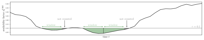
(a) Drought windows with fixed duration below a drought threshold $\tau=0.1$.

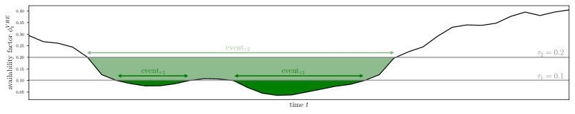
(b) Drought events with variable duration below two drought thresholds $\tau_{1}=0.1$ and $\tau_{1}=0.2$. Using higher thresholds generally leads to longer, but fewer, events.

Figure 2: Comparison of VRE drought definitions. The window perspective underestimates drought duration and overestimates the number of droughts.

Drought definition: window perspective. There are different definitions for VRE drought periods. One option is searching for ’drought windows’ with predefined duration [19, 33, 18], e.g., a given number of time steps below a given threshold (Figure 2a). Implementing a respective search algorithm for a specified window duration is straightforward. Yet, droughts identified via predefined windows may be shorter than actual droughts (Figure 2a). Further, consecutive windows that form one longer combined drought may be counted individually (Figure 2a, right windows). Thus, this definition systematically underestimates drought duration and overestimates the number of droughts.

Drought definition: event perspective. An alternative approach is searching for complete ’drought events’ below a threshold, which last as long as a drought qualification criterion is met. That is, drought duration is not predefined by setting a window length, but, for example, the result of a search on how many consecutive time steps are below a given threshold [25, 26, 17]. This ensures that identified events are completely captured, and consecutive droughts are properly accounted for (Figure 2b). We thus consider the drought event perspective to be a superior concept for identifying VRE droughts, and focus on it henceforward.

Threshold intuition. Higher thresholds generally identify less severe, but longer-lasting drought events. This tends to reduce the number of obtained droughts, as events that are considered to be separate for lower thresholds may integrate into combined ones (Figure 2b).

2.2 Drought identification methods

Identification method: CBT. Numerous methods exist for identifying VRE droughts. We focus on a selection in the following (Figure 3). A Constantly-Below-Threshold (CBT) event relates to a period of consecutive time steps during which availability factors are constantly below a threshold $\tau$ [50, 28, 22, 29, 30, 23, 17, 38]. In the hydrologic literature, this method has been first introduced as ’runs analysis’ [25]. The boolean function $\psi_{t}^{CBT}$ determines whether time step $t$ qualifies as drought (1) or not (0):

$$\psi_{t}^{CBT}=\begin{cases}1&\text{if $\phi_{t}^{VRE}<\tau\ \ \forall\ \ t$}\\ 0&\text{if $\phi_{t}^{VRE}\geq\tau\ \ \forall\ \ t$}\end{cases}$$ (1)

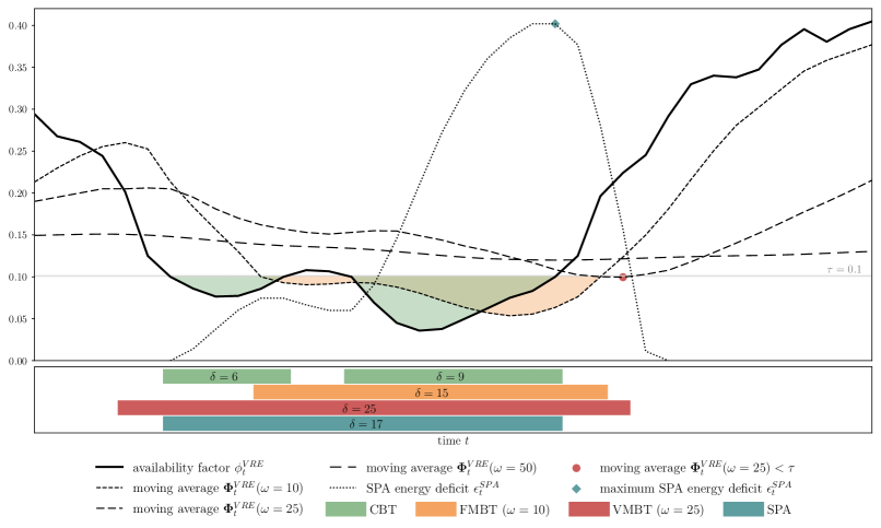
Figure 3: The upper panels shows exemplary VRE availability time series (bold line) and identification methods CBT, FMBT, VMBT, and SPA. The gray line represents the drought threshold $\tau=0.1$. Green and orange areas highlight the energy deficit obtained by CBT and FMBT, respectively. The lower panel’s horizontal bars illustrate the varying event duration $\delta$ identified by each method.

CBT duration & energy deficit. The duration of a CBT event $\delta^{CBT}$ is the number of consecutive time steps with $\psi_{t}^{CBT}=1$. Suppose $t_{k}$ and $t_{l}$ are the first and the last time steps of an event. Then the event’s cumulative energy, also referred to as energy deficit or drought severity [25, 17], is defined as follows:

$$\epsilon^{CBT}=\sum_{t_{k}}^{t_{l}}\tau-\phi_{t}^{VRE}\ \ \forall\ \ t_{k}\leq t\leq t_{l}$$ (2)

Limitation CBT. The CBT notion identifies VRE droughts regardless of availability factors in adjacent periods, even if their availability is briefly above the drought threshold (Figure 3).

Identification method: MBT. Addressing this limitation, Mean-Below-Threshold (MBT) events define consecutive time steps during which a moving average of availability factors $\Phi_{t}^{VRE}(\omega)$ is below a threshold [19, 30, 36, 37, 17]. This approach smooths out short-term fluctuations over the lagging averaging interval $[t-\omega,t]$ with a predefined duration $\omega$. Equivalent to $\psi_{t}^{CBT}$, the function $\psi_{t}^{MBT}$ evaluates each time step $t$ as follows:

$$\psi_{t}^{MBT}=\begin{cases}1&\text{if $\Phi_{t}^{VRE}(\omega)<\tau\ \ \forall\ \ t$}\\ 0&\text{if $\Phi_{t}^{VRE}(\omega)\geq\tau\ \ \forall\ \ t$}\end{cases}$$ (3)

Fixed-duration MBT. The MBT method can be applied in two different ways. First, the fixed-duration MBT (FMBT) searches for MBT events based on a fixed averaging interval $\omega^{FMBT}$ [36, 37, 17]. The duration of an FMBT event $\delta^{FMBT}$ corresponds to the number of consecutive time steps with $\psi_{t}^{FMBT}=1$ (e.g., $\delta^{FMBT}=15$ for $\omega=10$ in Figure 3). The energy deficit $\epsilon^{FMBT}$ is computed analogously to $\epsilon^{CBT}$ (i.e., using $\Phi_{t}^{VRE}(\omega)$ instead of $\phi_{t}^{VRE}$) and decreases due to the smoothing effect of the moving average. One option to avoid this is evaluating the energy deficit based on the original time series $\phi_{t}^{VRE}$ instead of $\Phi_{t}^{VRE}(\omega)$, i.e., reporting $\epsilon^{CBT}$ instead of $\epsilon^{FMBT}$ corresponding to the identified FMBT event [17].

Comparison CBT & FMBT. Unlike CBT, the FMBT approach allows for instances above the drought threshold before, between, and after potentially multiple CBT drought events that are filtered out by pooling them together (compare CBT and FMBT events in Figure 3) [17]. In the hydrology literature, such CBT events are referred to as ’mutually dependent’ [26]. For prolonging averaging intervals, the moving average smoothing becomes more pronounced. Hence, the choice of $\omega^{FMBT}$ determines to which extent shorter CBT events are filtered out. By design, for a given threshold, the CBT approach identifies more drought events than FMBT, whereas FMBT finds fewer but longer-lasting events. Thus, the CBT method may overestimate the number of drought events while underestimating the duration and energy deficit, which is particularly relevant for characterizing the cumulative energy of extreme VRE droughts. In contrast, the FMBT method acknowledges natural fluctuations in VRE availability by accounting for brief periods of higher availability within an overall low-availability period. FMBT therefore provides a more realistic view of prolonged VRE droughts and the corresponding power sector flexibility needs.

Limitation FMBT. However, there is no clear relation between a power sector attribute and $\omega^{FMBT}$, whose parameterization remains arbitrary. VRE availability time series could be evaluated for a range of different $\omega^{FMBT}$. Yet, drought events based on different $\omega^{FMBT}$ may partially overlap, creating ambiguity in their characteristics like duration, energy deficit, and frequency. In fact, results may substantially change with varying $\omega^{FMBT}$ (compare the moving averages $\Phi_{t}^{VRE}(\omega=10)$ and $\Phi_{t}^{VRE}(\omega=50)$ in Figure 3, with the latter obtaining no drought at all). Consequently, VRE droughts identified via the FMBT approach are valid only for a specific parameterization of $\omega^{FMBT}$, limiting the applicability of this concept.

Variable-duration MBT. Addressing this limitation, we introduce the variable-duration MBT (VMBT) method, which to the best of our knowledge is a novelty. It obtains unique VRE droughts, ranging from very long-lasting events, e.g., months, to such that last only a few time steps. This is achieved by deploying the MBT perspective for a large number of different averaging intervals, iteratively adjusting $\omega^{VMBT}$ in descending order. Importantly, to ensure that no long-duration events with $\delta^{VMBT}>\omega^{VMBT}$ are missed, the first iteration should start with a very high $\omega^{VMBT}$, so that the moving average $\Phi_{t}^{VRE}(\omega)>\tau$ across the entire time series (in the example shown in Figure 3, compare the moving average $\Phi_{t}^{VRE}(\omega^{VMBT}=50)$). In subsequent iterations, $\omega^{VMBT}$ is reduced and $\Phi_{t}^{VMBT}$ updated, until the first drought event is identified at $\Phi_{t}^{VMBT}<\tau$ (compare the moving average $\Phi_{t}^{VRE}(\omega=25)$ in Figure 3). Its duration equals the averaging interval $\delta^{VMBT}=\omega^{VMBT}$. The respective period is then excluded in later iterations, where $\omega^{VMBT}$ decreases further and additional (shorter) drought events are identified, and so on. For a given drought threshold $\tau$, this iterative process effectively captures all unique drought events, without any overlap or double counting, each accurately recorded with its maximum possible duration. Compared to FMBT, this renders the VMBT approach a more accurate and informative method for drought identification.

Limitation VMBT. Note that the VMBT energy deficit $\epsilon^{VMBT}$ is insignificant due to the close proximity of the moving average to the threshold. Further, this method involves a trade-off between accuracy and computational efficiency. Iteratively reducing the interval of the moving average ($\omega^{VMBT}$), with an incremental change that equals the resolution of the underlying time series, ensures captures all unique drought events, but requires numerous iterations and may lead to long processing time.

Identification method: SPA. Finally, the Sequent Peak Algorithm (SPA) identification method searches for the maximum cumulative energy deficit of a drought event, while accommodating intermediate periods where renewable availability may surpass the threshold. Originating in hydrology [51, 26], SPA has been extended to other bodies of literature, such as wind energy analysis [17]. A similar concept has also been applied to characterizing renewable surplus events [52]. The cumulative energy deficit is defined as follows:

$$\epsilon_{t}^{SPA}=\begin{cases}\epsilon^{SPA}_{t-1}+\tau-\phi_{t}^{VRE}&\text{if $\epsilon^{SPA}_{t-1}+\tau-\phi_{t}^{VRE}>0\ \ \forall\ \ t$}\\ 0&\text{if $\epsilon^{SPA}_{t-1}+\tau-\phi_{t}^{VRE}\leq 0\ \ \forall\ \ t$}\end{cases}$$ (4)

SPA duration. The SPA measures event duration $\delta^{SPA}$ from the first instance when the cumulative energy deficit of a single SPA event becomes positive to its global maximum. This maximum occurs when the VRE availability curve intersects with the threshold for the last time during an SPC event, i.e., when $\phi_{t}^{VRE}\geq\tau$ (Figure 3). This algorithm requires no iterations or assumptions on averaging intervals, and only a single straightforward computation of cumulative energy deficits for the underlying VRE availability time series. It allows for long-duration events that include brief periods with above-threshold availability.

Comparison SPA & VMBT: Unlike VMBT, SPA events start when VRE availability falls below the threshold and thus depends on threshold parameterization. In contrast, the VMBT method allows for high or low availability periods before SPA events, making it less reliant on specific threshold parameterization. For a given threshold, both VMBT and SPA obtain a unique and unambiguous set of VRE drought events, and thus appear to be superior to the CBT of FMBT approaches. SPA is computationally less demanding than VMBT, as it requires no iterations over averaging intervals. Yet, SPA may not recognize minor events that follow a longer-lasting drought, which has been criticized in the literature [17].

Comparison duration CBT, FMBT, VMBT, SPA. As indicated by Figure 3, for a given threshold, the VMBT approach generally leads to the longest drought duration of all four identification strategies explained above. The SPA method identifies events with extended duration, albeit shorter than VMBT, followed by FMBT events with moderate duration. On the other end of the spectrum, the CBT method leads to the shortest drought duration.

Limitation of energy deficits in VRE drought analysis. While often reported in other bodies of literature, energy deficits of VRE droughts identified purely based on VRE availability are hard to interpret as they do not allow for drawing direct energy system conclusions.

Threshold parameterization. Note that an effective threshold parameterization is methodologically challenging and subject to user discretion (see Section 2.3 for further discussion).

2.3 Comparability and the choice of threshold

Comparability issues. Research interest is increasingly moving beyond single technologies at particular regions (e.g., [22, 23, 24, 27, 30]) towards a characterization of VRE drought patterns of portfolios of different renewable generation technologies for multiple regions (e.g., [19, 18, 32, 33]). For this, enabling comparability across VRE technologies and regions when analyzing VRE drought events is imperative.

Differences in generation potentials: single technologies. Previous research draws on absolute, exogenously set thresholds for availability factors, e.g., 0.01, 0.02, 0.05, or 0.10 [28, 29, 36, 30, 32, 17]. Yet, such analyses face compatibility issues when analyzing systems with different technologies and/or across several regions. This is because applying absolute thresholds on normalized availability factor time series implies assuming uniform generation capacity (e.g., in megawatts) across all compared systems. However, these systems may have very different annual generation potentials (e.g., in megawatt hours) depending on the meteorological conditions of the location and the VRE technology. VRE availability duration curves, sorting availability factor time series in descending order, highlight the discrepancies in generation potentials between different technologies and regions (Figure 4a).

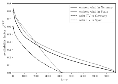
(a) Availability duration curves of single VRE technologies.

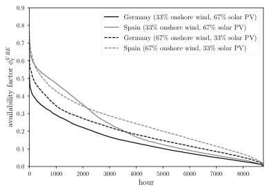
(b) Availability duration curves of VRE portfolios with different exemplary capacity mixes.

Figure 4: Annual generation potentials of onshore wind power, solar PV, and portfolios with different mixes of these technologies in Germany and Spain in 2010, visualized as the area below the availability duration curves. The data is retrieved from the Pan-European Climate Database [53].

Differences in generation potentials: technology portfolios. The same applies to energy systems transitioning towards variable renewables. Here, the optimal capacity mix of VRE technologies depends on their respective generation potentials as well as cost parameters, and may vary substantially across regions. This results in diverse generation potentials for such VRE portfolios based on the location and the capacity mix (Figure 4b).

Challenges with absolute thresholds: FLH bias. Full-load hours (FLH) serve as a commonly used metric for comparing annual average generation (or generation potential before potential curtailment). This metric indicates how long a generator (or technology aggregate) would operate at full capacity to provide its annual energy (potential). An analysis based on a uniform, exogenously set threshold for each compared system does not account for discrepancies in annual generation potentials. Consequently, such analyses (e.g., [36, 32, 39, 38]) are biased by a FLH effect, which puts their validity into question.

Threshold scaling relative to maximum availability factor. As a remedy, the drought threshold can be scaled to account for FLH differences between VRE technologies and locations. Threshold scaling relative to different time series attributes can be found in the literature. One option is to scale thresholds relative to their system-specific maximum availability factor [35].. Focusing on the VRE availability of a single point in time (i.e., the peak point of the duration curves in Figure 4), this approach ignores general availability patterns over the course of a year. Consequently, it does not mitigate differences in FLH.

Thresholds scaling relative to the distribution of availability factors. Another option is to use a percentile of the availability time series distribution as threshold [26, 22, 45]. Duration curves are a graphical representation of availability factor distributions (Figure 4). A percentile refers to the availability factor below a certain fraction of the population of time steps falls and depends on the shape of the distribution, which may vary across technologies and regions. Unlike scaling relative to the maximum availability factor, this method recognizes all VRE availability states. However, the percentile approach does not fully adjust for FLH differences.

Thresholds scaling relative to mean availability factor. An effective option for this is to align the drought threshold with each system’s mean availability factor $\bar{\phi}^{VRE}$. This method inherently scales with the system’s FLH and, therefore, enables comparability across technologies or technology portfolios, regions, and, in the case of comparing multiple years, time [19, 18, 31, 40, 33].

Effective threshold ranges. A priori, a meaningful parameterization of the fraction $\alpha$ of the mean availability factor $\bar{\phi}^{VRE}$ for drought identification is not straightforward. Previous studies use various fractions of the mean [25]. While lower thresholds, e.g., $\tau=0.1\bar{\phi}^{VRE}$, find very severe but potentially brief and isolated VRE drought events, higher fractions closer to $\bar{\phi}^{VRE}$ may result in identifying extended periods of below-average availability rather than true VRE droughts. Relevant fractions likely lie between these extremes. It therefore appears useful to explore a range of thresholds, $\tau=\alpha*\bar{\phi}^{VRE}$, for example with $\alpha$ ranging between 0.1 and 0.9. Obtained events reflect different degrees of low VRE availability, which may be relevant for different types of flexibility options in renewable energy systems.

2.4 Technological and spatial scope of analysis

VRE drought analyses scopes. The scope of a VRE drought analysis focusing on VRE supply may differ in terms of technological and spatial scope. Each of these dimensions demands specific assumptions, weighting, as well as comparability requirements.

Portfolio time series in multi-technology analyses. In contrast to single-technology drought analyses, according investigations of a VRE portfolio require a composite time series that combines the availability factors of different VRE technologies. It can be computed as the weighted average of the technology-specific time series. Weighting factors correspond to the technology shares in the assumed overall capacity mix. Considering the temporal and spatial complementarity of wind and solar power [54, 55], such a composite time series allows for within-portfolio balancing, which reflects the generation dynamics of power sectors with high shares of variable renewables. This is in line with several related studies [19, 43, 20, 44]. Another approach excludes or limits such balancing by applying a definition of compound VRE drought events as periods with simultaneously arising drought conditions of multiple VRE technologies [18, 38]. This discards VRE complementarity, hence potentially overestimating droughts characteristics of a VRE portfolio.

Interconnection states in multi-regional analysis. For multi-regional settings, drought analyses using VRE availability time series can be based on two extreme scenarios regarding regional interconnection: i) perfect interconnection, which abstracts from grid limitations (often referred to as the “copper plate” assumption), and ii) complete isolation, where regions are treated as “island systems” without electricity exchange. When comparing VRE droughts of such island systems, FLH-adjusted threshold scaling is required as discussed above. Realistic patterns of cross-regional electricity exchange fall between these extremes and typically necessitate more sophisticated energy system modeling beyond simple VRE time series analysis.

Cross-regional time series. Similar to the technology portfolio case, multi-regional settings with assumed perfect interconnection require a composite time series that collectively represents all regions. It can be generated as the weighted average of respective regional time series. The weights are assigned based on the relative share of each region’s capacity within the overall system. Unless multiple cross-regional composite time series are to be compared, no FLH-adjustment of the threshold is required. For VRE portfolios across regions, weighting factors need to reflect both within-regional and across-regional shares in the capacity mixes.

3 Extending the methodology to positive residual load events

3.1 Positive residual load event definition

Motivation: kalte Dunkelflauten. In addition to focusing exclusively on VRE supply, research interest on the dynamics between VRE droughts and periods of high electricity demand is intensifying. This becomes more relevant as many countries plan to electrify their heat, transport, and industry sectors, and respective additional loads enter the power sector. Notably during the heating season, electrified heating appliances such as heat pumps increase electricity demand with characteristic profiles [56, 57, 58]. Compound high-demand and VRE drought events, sometimes also referred to as “cold dark doldrums” or, in German, “kalte Dunkelflauten” are emerging as a challenge for decarbonized energy systems that rely on VRE.

Positive & negative residual load events. PRL events, characterized by high demand and a shortage of VRE supply, indicate the need for firm capacity from thermal generators, or flexibility provided by electricity storage, imports, or demand-side measures [59, 60, 61]. In contrast, negative residual load events represent VRE surplus generation. This surplus can be integrated into the power sector through electricity storage or exports to other areas, or used for electrified loads from coupled sectors, such as heat provision or transport [62]. Alternatively, it can be curtailed [52, 60]. Note that the latter is not an option for PRL periods, which makes them more challenging to deal with than negative residual loads. Accurately quantifying both positive and negative residual load events is relevant for capacity planning of weather-resilient energy systems.

PRL characteristics. Key PRL characteristics, e.g., duration and energy deficits, can be analyzed using residual load time series $\phi_{t}^{RL}$ (Figure 5). While this can be done analogously to VRE drought analysis, the energy deficit of PRL events can directly be associated with the need for energy that has to be provided by, for instance, long-duration storage. Importantly, the maximum capacity need can be inferred from peak residual load (compare left-most value of the residual load duration curve in Figure 5) and does not require a dedicated analysis of PRL events.

Implicit threshold parameterization. Unlike VRE drought analysis, there is no need for deliberate threshold parameterization to identify PRL events. Instead, PRL events are simply obtained as periods above zero (gray line in Figure 5). In previous PRL analysis other approaches such as percentile-based thresholds were used [40]. However, positive residual load directly relates to the need for energy from firm generators, storage, or imports. Hence, from the perspective of a power sector, diverting from thresholds aligned with the zero line appears counter-intuitive.

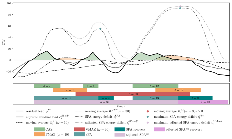
Figure 5: Exemplary residual load time series and identification methods CAZ, FMAZ, VMAZ, SPA (with or without recovery), and SPA^adj (upper panel). The green and orange areas indicate the obtained CAZ and FMAZ energy deficit, respectively. The lower panel’s horizontal bars illustrate the varying event duration $\delta$ identified by each method.

3.2 Identification methods

Identification methods: CAZ & MAZ. We adapt the VRE droughts identification methods discussed in Section 2 to PRL events. Unless stated otherwise, the algorithmic routine is equivalent but recalibrated to identify periods where residual load $\phi_{t}^{RL}$, or its average $\Phi_{t}^{RL}$, is above zero, rather than below a designated threshold. Analogously to CBT and MBT, we denote Constantly-Above-Zero (CAZ) and Mean-Above-Zero (MAZ) as:

$$\psi_{t}^{CAZ}= \begin{cases}1&\text{if $\phi_{t}^{RL}>0\ \ \forall\ \ t$}\\ 0&\text{if $\phi_{t}^{RL}\leq 0\ \ \forall\ \ t$}\end{cases} \psi_{t}^{FMAZ}= \begin{cases}1&\text{if $\Phi_{t}^{RL}(\omega)>0\ \ \forall\ \ t$}\\ 0&\text{if $\Phi_{t}^{RL}(\omega)\leq 0\ \ \forall\ \ t$}\end{cases}$$ (5)

Identification methods: FMAZ & VMAZ. Accordingly, the fixed-duration MAZ (FMAZ) and variable-duration MAZ (VMAZ) concepts emulate the FMBT and VMBT approaches.

Duration CAZ, FMAZ, VMAZ.. Analogously to VRE drought analysis, the PRL event duration $\delta^{CAZ}$ and $\delta^{FMAZ}$ corresponds to the number of consecutive time steps with $\psi_{t}^{CAZ}=1$ and $\psi_{t}^{FMAZ}=1$, respectively. The duration of VMAZ event equals the iteration-specific averaging interval $\delta^{VMAZ}=\omega^{VMAZ}$.

Energy deficit CAZ, FMAZ, VMAZ. The VMAZ energy deficit is near zero and hence insignificant. With $t_{k}$ and $t_{l}$ as the start and end points of a PRL event, the CAZ and FMAZ event’s energy deficit (green and orange areas in Figure 5) are defined as:

$$\epsilon^{CAZ}= \sum_{t_{k}}^{t_{l}}\phi_{t}^{RL} \epsilon^{FMAZ}= \sum_{t_{k}}^{t_{l}}\Phi_{t}^{RL} \forall\ \ t_{k}\leq t\leq t_{l}$$ (6)

Limitations of CAZ, FMAZ, and VMAZ. The limitations associated with CBT, FMBT, and VMBT discussed in Section 2 also extend to their PRL counterparts. The CAZ method, while directly linking event duration, its energy deficit, and its temporal occurrence to for example the required generation and dispatch period of a capacity-constrained firm generator, ignores brief periods of negative residual load adjacent to PRL events (compare the two CAZ events on the left in Figure 5). This can lead to underestimating the need for energy-constrained flexibility options, such as long-duration electricity storage. As for FMAZ, the parameterization of the averaging interval $\omega^{MAZ}$ lacks a directly attributable power sector reference and remains arbitrary. As identified FMAZ events may substantially change with varying $\omega^{MAZ}$, they are ambiguous. Further, their interpretation is not straightforward. In general, longer averaging periods may lead to an underestimation of actual PRL challenges as averaging already assumes temporal balancing, for instance, in real-world power systems carried out by electricity storage or other flexibility options. The VMAZ approach, in contrast, obtains unique events. Yet, its relevance remains limited in PRL analysis as it only allows for evaluating PRL event duration but not energy deficit, which converges to zero by design.

Identification method: SPA. The SPA identifies unique PRL while obtaining a meaningful energy deficit. Unlike for VRE droughts, SPA does not require setting an arbitrary threshold for PRL detection, precluding a respective shortcoming in the case of VRE drought identification. SPA allows for brief periods with negative residual load and detects all PRL events within a single iteration. Consequently, we regard it as particularly well-suited for identifying PRL events. Analogously to VRE droughts, its cumulative energy deficit is denoted as:

$$\epsilon_{t}^{SPA}=\begin{cases}\epsilon^{SPA}_{t-1}+\phi_{t}^{RL}&\text{if $\epsilon^{SPA}_{t-1}+\phi_{t}^{RL}>0\ \ \forall\ \ t$}\\ 0&\text{if $\epsilon^{SPA}_{t-1}+\phi_{t}^{RL}\leq 0\ \ \forall\ \ t$}\end{cases}$$ (7)

SPA duration and recovery period. The SPA event duration $\delta^{SPA}$ refers to the period beginning when the cumulative energy deficit of a single SPA event becomes positive to its global maximum. The SPA method further allows for quantifying a recovery period $\sigma^{SPC}$. Originating from the hydrology field [63], this period represents the balancing time required for the surplus VRE energy from intermediate and subsequent negative residual load events to offset the energy deficit of a PRL event. It corresponds to the period following the peak cumulative energy deficit $\epsilon_{t}^{SPA}$ to the point in time where this deficit returns to zero $\epsilon_{t}^{SPC}=0$ (Figure 5).

Accounting for efficiency losses: adjusted SPA. In real-world energy systems, long-duration electricity storage is a key option for dealing with PRL events [20]. Storage always incurs conversion losses, i.e., the amount of electricity recovered from storage is always smaller than previous storage charging. The standard SPA method does not account for such losses. To address this, we introduce an adjusted Sequent Peak Algorithm (SPA^adj) method, which incorporates storage efficiency losses arising when balancing positive and negative residual load periods. This can be achieved by adjusting all negative residual load values to account for storage round-trip efficiency $\eta^{LDS}$ as denoted by:

$$\phi_{t}^{RL,adj}=\frac{\phi_{t}^{RL}}{\eta^{LDS}}\ \ \forall\ \ \phi_{t}^{RL}<0$$ (8)

Adjusted recovery period. In the SPA^adj method, the adjusted energy deficit $\epsilon_{t}^{SPA,adj}$ is calculated equivalently to $\epsilon_{t}^{SPA}$. However, assuming that long-duration electricity storage is the relevant flexibility option for dealing with a PRL event, the round-trip efficiency adjustment prolongs the recovery period $\sigma^{SPA,adj}$ to reflect the time needed to recharge the storage to its pre-PRL state of charge (Figure 5). This approach results in an extended recovery period $\sigma^{SPA,adj}$ and event duration $\delta^{SPC}$ when compared to calculations without considering efficiency losses. This adjustment leads to a more realistic representation of the energy system flexibility need during compound peak demand and VRE drought events. Note that real-world storage options may also incur relevant standing losses, depending on how long the energy is stored. Incorporating these into the SPA concept would be significantly increase complexity and should rather be studied using appropriate energy models.

3.3 Comparability, scope of analysis, and critical appraisal

Implicit comparability. Unlike VRE droughts, analyzing PRL events does not require pre-processing, such as a FLH adjustment, to enable comparability. PRL events are denoted in energy (e.g., megawatt hours), which is readily comparable across different technological, spatial, and temporal scopes.

Setting: Exogenous residual load. The analysis of residual load time series can be approached in two ways. On option is to use exogenous assumptions for both VRE availability factors and demand time series. This setup facilitates the exploration of various user-specific VRE capacity mix scenarios.

Setting: Optimized residual load. Alternatively, residual load time series can be retrieved from a scenario optimized by an energy system model. This method is more resource-intensive due to the need for comprehensive input data and complex modeling assumptions, but also less dependent on exogenous capacity assumptions. It further enables an analysis of policy-relevant scenarios, such as those outlined in strategic documents like the Ten Year Network Development Plan for the European electricity infrastructure [64].

Interpretation of PRL characteristics. Characterizing extreme PRL events, i.e., their duration, energy deficit, frequency, etc., allows exploring the need for power sector flexibility, which can be provided by long-duration storage or other flexibility options. The SPA^adj, accounting for energy losses of such flexibility options, appears to be particularly useful in this respect.

General Limitation. During an extreme PRL events, brief periods with very high VRE generation requiring partial curtailment may occur. None of the discussed identification methods is able to account for such curtailed energy, which can lead to underestimating the energy deficit and duration of extreme PRL events [20]. More importantly, insights from PRL event analysis are only applicable to specific assumptions on the VRE portfolio and load, or driven by the parameterization of optimizing models. Therefore, when discussing characteristics such as the duration, frequency, or energy deficit of PRL events, contextualization is essential. This is particularly important for a meaningful comparison of the findings of different studies, and for communication with policy-makers or the general public.

Limitations: exogenous residual load. By design, an exogenously derived residual load time series does not account for electricity exchange and potentially neglects flexibility from conventional demand and electrified loads from the heating, transport, or industry sector. Accurately estimating the operation of these loads without the use of an energy system model is challenging and may require numerous assumptions.

Limitations: optimized residual load. As for residual load time series generated by optimizing energy system models, model outcomes rely on the used modeling framework and its underlying optimization rationale, the level and detail of technology representation, and techno-economical assumptions, such as available technologies, costs, meteorological resources [65, 66, 67]. For instance, ceteris paribus, changes in storage investment costs can significantly affect storage investment and usage in a modeled scenario, thus altering the energy deficit or duration of obtained PRL events.

Note that an optimized residual load resulting from energy system modeling already takes into account the optimal capacities and dispatch decisions of electricity storage and other flexibility options. This inherently affects PRL event characteristics.

4 Conclusion and recommendations

4.1 Contribution

Gap in literature & suggested terminology. VRE shortage has drawn research interest from various fields, including hydrology, wind and solar energy, energy system modeling, or climatology, and has been analyzed using a range of methods and disparate naming. Yet, there is no structured overview and explanation of these methods using harmonized terminology. It thus remains unclear as to what methodological approach is useful for different settings of VRE shortage analysis, which can be studied based on time series of VRE availability or positive residual load. For clarity, we suggest “variable renewable energy shortage” as a generic term covering both “variable renewable droughts” as periods with low resource availability of a single or multiple VRE technologies and “positive residual load events” as periods with a net imbalance of electric load and VRE supply.

Contribution. This paper addresses this gap by providing a methodological overview and guidance for defining and quantifying VRE shortage events across technologies and regions, discussing different approaches for both VRE availability and PRL time series. While not claiming to be exhaustive, we categorize and discuss relevant existing shortage event definitions and identification methods, propose methodological improvements, and elaborate on how to enable compatibility in cross-technology or multi-regional analyses. Our work seeks to support the harmonization of terminology across related fields. We also aim to aid in advancing future research on VRE shortage events by facilitating a better interpretation of such studies’ potential findings.

4.2 What (not) to do in variable renewable energy shortage analysis

Good practices. We identify a range of good practices for VRE shortage analysis to obtain accurate, broadly applicable, and easy-to-interpret findings on the duration, frequency, and energy deficit of VRE shortage events. This is important for guiding policy or infrastructure decisions for future energy systems with high VRE penetration.

Good practices: specify method. We advocate for future work to clearly and unambiguously specify the shortage period definitions and identification methods used, as well as key parameter choices such as thresholds or averaging intervals. Methods that are poorly defined or not transparent hinder the accurate interpretation and contextualization of findings, in both research and policy discourse.

Good practice: methodical requirements. For accurate identification, VRE shortage analysis should meet a range of methodological criteria. First, VRE shortage periods should be defined according to the event perspective, i.e., capturing the full extent of qualifying periods allowing for event duration ranging from just a few time steps to extensive weeks or even months. Second, identified shortage events should be unique, avoiding double counting and overlap with adjacent events. Third, the method should allow for pooling of closely occurring events to include periods that independently may not qualify as VRE drought or PRL events but are adjacent to periods of low availability or high residual load.

Good practice: recommended VRE shortage characteristics. In general, reporting the VRE shortage duration appears to be equally relevant to VRE drought and PRL analyses. Yet, claims on identified durations have to be contextualized, as they depend on the identification method used. Further, evaluating energy deficits of PRL events is valuable for understanding the demand for firm generation or long-duration storage energy in renewable power sectors. Conversely, even tho this metric is commonly applied in VRE drought analysis across different bodies of literature, it appears to be less relevant in such settings, as it strongly depends on the threshold parameter choice and cannot be associated with a power sector attribute.

Good practice: recommended methods. For VRE droughts analysis, the VMBT and SPA methods align well with these methodological requirements. The VMBT method finds events with the longest duration but lacks meaningful energy deficits, which is a reasonable cost for accurate duration identification. In the case of PRL analyses, we recommend the use of SPA or its adjusted version, SPA^adj. Besides adhering to the outlined criteria, these methods allow for accurately quantifying both duration and the energy deficit of PRL events.

Good practice: comparative analyses. Analyzing VRE droughts across multiple regions and/or for different VRE technologies or technology portfolios poses comparability challenges. It is essential to base the analysis on uniform average generation (or generation potential) across compared systems to avoid a FLH bias in obtained drought characteristics. Threshold scaling for each investigated system according to a fraction of the mean capacity factors is an effective option for enabling comparability.

Good practice: threshold selection. The selection of the respective fraction remains a sensitive parameter choice and requires careful consideration. Too high thresholds may identify long-lasting periods with below-average VRE availability rather than actual VRE droughts. Conversely, very low thresholds may find very severe but potentially brief and isolated droughts. We advise exploring various threshold values between these extremes, ranging from near-zero to the average availability factor. This ensures a comprehensive capture of the full spectrum of drought events, from mild to very severe.

Good practices: open code and data. For transparency and reproducibility, it further appears vital to document and provide the underlying data and the algorithms used, adhering to open-source and open-data principles [68]. Such practices will not only foster transparency and replicability, but also strengthen the overall accuracy and practical usefulness of VRE drought analyses.

Bad practices. Based on our analysis, we identify a range of bad practices for VRE shortage analysis. Searching for fixed-duration shortage windows underestimates shortage duration while inflating the number of identified shortage periods. We thus strongly recommend not using the window perspective. Methods yielding ambiguous sets of events that may change for varying method parameterization, such as FMBT and FMAZ, should be avoided due to the limited applicability of obtained shortage characteristics. Next, we advise against the use of methods incapable of pooling mutually dependent shortage events, such as CBT and CAZ, as obtained results overestimate the number of events while underestimating event duration and energy deficit. Finally, in VRE drought studies, using absolute thresholds can further lead to misleading comparisons based on normalized generation capacities rather than actual energy production, resulting in potentially flawed conclusions.

4.3 Methodological trade-offs and outlook

Trade-offs between VRE drought and PRL analysis. Renewable energy shortage can be studied based on time series of VRE availability or positive residual load. While both approaches have their merits, a trade-off between policy relevance and the universality of insights emerges. VRE drought analysis based on VRE availability data typically requires fewer assumptions, yielding conclusions with broader applicability. PRL events analyses aim to be more policy-oriented, as they quantify the mismatch between electricity demand and VRE supply, which is especially relevant for highly renewable decarbonization scenarios. However, the latter approach requires extensive assumptions on the composition of the renewable generation portfolio and demand-side flexibility. This may necessitate detailed energy system modeling, whose outcomes hinge upon underlying optimization rationales, technology representation, and parameterization. This potentially limits the validity of PRL analyses to the particular scenarios investigated.

Trade-offs between single and multiple technologies VRE drought analysis. Such a trade-off also applies to the technological scope of VRE drought analysis. Aside from methodological assumptions inherent to the generation of VRE availability time series, e.g., such for reanalysis, insights from single-technology analysis are broadly applicable but less policy-relevant for future energy systems that rely on a mix of VRE technologies. Conversely, analyzing a VRE portfolio is more policy-oriented but involves energy modeling or exogenous assumptions on the composition of the investigated capacity mix. VRE capacity mixes determined by an energy modeling are optimal only in the context of the other optimized system components and flexibility options that are represented in the model (e.g., storage, electricity exchange, or direct-electrified applications from the heat, industry, or transport sector). Similarly, exogenous capacity mixes rely on user-specific assumptions. These aspects limit the validity of insights to investigated scenarios.

Outlook. While we provide general guidance on the advantages and drawbacks of different VRE shortage identification methods, a thorough quantitative comparison would be desirable, ideally for a range of VRE technologies and electric load profiles for different world regions and weather years. Another key aspect that requires attention is the choice of the threshold parameter, particularly in distinguishing between severe VRE droughts and prolonged periods of below-average availability. This distinction could support the selection of relevant weather years to enable weather- and climate-resilient energy system analyses and well-informed decarbonization policies. Additionally, assessing the sensitivity of outcomes to different VRE availability datasets would be useful and could be valuable feedback to the meteorological research community that provides and continuously improves such datasets [47].

Author Contributions

Martin Kittel: Conceptualization (equal), methodology, software, investigation, data curation, visualization, writing - original draft, review and editing (equal). Wolf-Peter Schill: Conceptualization (equal), writing - review and editing (equal), project administration.

References

-
[1]
K. Calvin, D. Dasgupta, G. Krinner, A. Mukherji, P. W. Thorne, C. Trisos, J. Romero, P. Aldunce, K. Barrett, G. Blanco, W. W. Cheung, S. Connors, F. Denton, A. Diongue-Niang, D. Dodman, M. Garschagen, O. Geden, B. Hayward, C. Jones, F. Jotzo, T. Krug, R. Lasco, Y.-Y. Lee, V. Masson-Delmotte, M. Meinshausen, K. Mintenbeck, A. Mokssit, F. E. Otto, M. Pathak, A. Pirani, E. Poloczanska, H.-O. Pörtner, A. Revi, D. C. Roberts, J. Roy, A. C. Ruane, J. Skea, P. R. Shukla, R. Slade, A. Slangen, Y. Sokona, A. A. Sörensson, M. Tignor, D. Van Vuuren, Y.-M. Wei, H. Winkler, P. Zhai, Z. Zommers, J.-C. Hourcade, F. X. Johnson, S. Pachauri, N. P. Simpson, C. Singh, A. Thomas, E. Totin, P. Arias, M. Bustamante, I. Elgizouli, G. Flato, M. Howden, C. Méndez-Vallejo, J. J. Pereira, R. Pichs-Madruga, S. K. Rose, Y. Saheb, R. Sánchez Rodríguez, D. Ürge Vorsatz, C. Xiao, N. Yassaa, A. Alegría, K. Armour, B. Bednar-Friedl, K. Blok, G. Cissé, F. Dentener, S. Eriksen, E. Fischer, G. Garner, C. Guivarch, M. Haasnoot, G. Hansen,
M. Hauser, E. Hawkins, T. Hermans, R. Kopp, N. Leprince-Ringuet, J. Lewis, D. Ley, C. Ludden, L. Niamir, Z. Nicholls, S. Some, S. Szopa, B. Trewin, K.-I. Van Der Wijst, G. Winter, M. Witting, A. Birt, M. Ha, J. Romero, J. Kim, E. F. Haites, Y. Jung, R. Stavins, A. Birt, M. Ha, D. J. A. Orendain, L. Ignon, S. Park, Y. Park, A. Reisinger, D. Cammaramo, A. Fischlin, J. S. Fuglestvedt, G. Hansen, C. Ludden, V. Masson-Delmotte, J. R. Matthews, K. Mintenbeck, A. Pirani, E. Poloczanska, N. Leprince-Ringuet, C. Péan, IPCC, 2023: Climate Change 2023: Synthesis Report. Contribution of Working Groups I, II and III to the Sixth Assessment Report of the Intergovernmental Panel on Climate Change [Core Writing Team, H. Lee and J. Romero (eds.)]. IPCC, Geneva, Switzerland., Tech. rep., Intergovernmental Panel on Climate Change (IPCC), edition: First (Jul. 2023).
doi:10.59327/IPCC/AR6-9789291691647.
URL https://www.ipcc.ch/report/ar6/syr/ -
[2]
P. Denholm, M. Hand, Grid flexibility and storage required to achieve very high penetration of variable renewable electricity, Energy Policy 39 (3) (2011) 1817–1830.
doi:10.1016/j.enpol.2011.01.019.
URL https://linkinghub.elsevier.com/retrieve/pii/S0301421511000292 -
[3]
M. G. Rasmussen, G. B. Andresen, M. Greiner, Storage and balancing synergies in a fully or highly renewable pan-European power system, Energy Policy 51 (2012) 642–651.
doi:10.1016/j.enpol.2012.09.009.
URL https://linkinghub.elsevier.com/retrieve/pii/S0301421512007677 -
[4]
D. Schlachtberger, T. Brown, S. Schramm, M. Greiner, The benefits of cooperation in a highly renewable European electricity network, Energy 134 (2017) 469–481.
doi:10.1016/j.energy.2017.06.004.
URL https://linkinghub.elsevier.com/retrieve/pii/S0360544217309969 -
[5]
A. Roth, W.-P. Schill, Geographical balancing of wind power decreases storage needs in a 100% renewable European power sector, iScience 26 (7) (2023) 107074.
doi:10.1016/j.isci.2023.107074.
URL https://linkinghub.elsevier.com/retrieve/pii/S2589004223011513 -
[6]
G. He, D. S. Mallapragada, A. Bose, C. F. Heuberger-Austin, E. Gençer, Sector coupling via hydrogen to lower the cost of energy system decarbonization, Energy & Environmental Science 14 (9) (2021) 4635–4646.
doi:10.1039/D1EE00627D.
URL http://xlink.rsc.org/?DOI=D1EE00627D -
[7]
D. Kirchem, W.-P. Schill, Power sector effects of green hydrogen production in Germany, Energy Policy 182 (2023) 113738.
doi:10.1016/j.enpol.2023.113738.
URL https://linkinghub.elsevier.com/retrieve/pii/S0301421523003233 - [8] L. C. Dawkins, I. Rushby, Characterising Adverse Weather for the UK Electricity System, Tech. rep., MetOffice (2020).
-
[9]
F. Huneke, C. Perez Linkenheil, M. Niggemeier, Kalte Dunkelflaute Robustheit des Stromsystems bei Extremwetter, Tech. rep., Energy Brainpool, Berlin (2017).
URL https://www.energybrainpool.com/de/downloads -
[10]
DHU, Hintergrundpapier: Versorgungssicherheit mit 100% Erneuerbaren Energien, Tech. rep., Deutsche Umwelthilfe, Berlin (2021).
URL https://www.duh.de/fileadmin/user_upload/download/Projektinformation/Erneuerbare_Energien/DUH_Hintergrundpapier_Versorgungssicherheit_Nov21.pdf - [11] D. Bundestag, Sicherstellung der Stromversorgung bei Dunkelflauten, Tech. rep., Deutscher Bundestag, Berlin (Jan. 2019).
- [12] T. Wood, J. Ha, Go for net zero, Tech. rep., Grattan Institute (2021).
- [13] J. Novacheck, J. Sharp, M. Schwarz, P. Donohoo-Vallett, Z. Tzavelis, G. Buster, M. Rossol, The Evolving Role of Extreme Weather Events in the U.S. Power System with High Levels of Variable Renewable Energy, Tech. Rep. NREL/TP-6A20-78394, National Renewable Energy Laboratory, Golden, CO (2021).
-
[14]
J. A. Dowling, K. Z. Rinaldi, T. H. Ruggles, S. J. Davis, M. Yuan, F. Tong, N. S. Lewis, K. Caldeira, Role of Long-Duration Energy Storage in Variable Renewable Electricity Systems, Joule 4 (9) (2020) 1907–1928.
doi:10.1016/j.joule.2020.07.007.
URL https://linkinghub.elsevier.com/retrieve/pii/S2542435120303251 -
[15]
N. A. Sepulveda, J. D. Jenkins, A. Edington, D. S. Mallapragada, R. K. Lester, The design space for long-duration energy storage in decarbonized power systems, Nature Energy 6 (5) (2021) 506–516.
doi:10.1038/s41560-021-00796-8.
URL https://www.nature.com/articles/s41560-021-00796-8 -
[16]
P. T. Brown, D. J. Farnham, K. Caldeira, Meteorology and climatology of historical weekly wind and solar power resource droughts over western North America in ERA5, SN Applied Sciences 3 (10) (2021) 814.
doi:10.1007/s42452-021-04794-z.
URL https://link.springer.com/10.1007/s42452-021-04794-z -
[17]
P. Potisomporn, T. A. Adcock, C. R. Vogel, Extreme value analysis of wind droughts in Great Britain, Renewable Energy 221 (2024) 119847.
doi:10.1016/j.renene.2023.119847.
URL https://linkinghub.elsevier.com/retrieve/pii/S0960148123017627 -
[18]
K. Z. Rinaldi, J. A. Dowling, T. H. Ruggles, K. Caldeira, N. S. Lewis, Wind and Solar Resource Droughts in California Highlight the Benefits of Long-Term Storage and Integration with the Western Interconnect, Environmental Science & Technology 55 (9) (2021) 6214–6226.
doi:10.1021/acs.est.0c07848.
URL https://pubs.acs.org/doi/10.1021/acs.est.0c07848 -
[19]
D. Raynaud, B. Hingray, B. François, J. Creutin, Energy droughts from variable renewable energy sources in European climates, Renewable Energy 125 (2018) 578–589.
doi:10.1016/j.renene.2018.02.130.
URL https://linkinghub.elsevier.com/retrieve/pii/S0960148118302829 -
[20]
O. Ruhnau, S. Qvist, Storage requirements in a 100% renewable electricity system: extreme events and inter-annual variability, Environmental Research Letters 17 (4) (2022) 044018.
doi:10.1088/1748-9326/ac4dc8.
URL https://iopscience.iop.org/article/10.1088/1748-9326/ac4dc8 -
[21]
K. van der Wiel, H. C. Bloomfield, R. W. Lee, L. P. Stoop, R. Blackport, J. A. Screen, F. M. Selten, The influence of weather regimes on European renewable energy production and demand, Environmental Research Letters 14 (9) (2019) 094010.
doi:10.1088/1748-9326/ab38d3.
URL https://iopscience.iop.org/article/10.1088/1748-9326/ab38d3 -
[22]
D. Cannon, D. Brayshaw, J. Methven, P. Coker, D. Lenaghan, Using reanalysis data to quantify extreme wind power generation statistics: A 33 year case study in Great Britain, Renewable Energy 75 (2015) 767–778.
doi:10.1016/j.renene.2014.10.024.
URL https://linkinghub.elsevier.com/retrieve/pii/S096014811400651X -
[23]
P. Potisomporn, C. R. Vogel, Spatial and temporal variability characteristics of offshore wind energy in the United Kingdom, Wind Energy 25 (3) (2022) 537–552.
doi:10.1002/we.2685.
URL https://onlinelibrary.wiley.com/doi/10.1002/we.2685 -
[24]
P. Potisomporn, T. A. Adcock, C. R. Vogel, Evaluating ERA5 reanalysis predictions of low wind speed events around the UK, Energy Reports 10 (2023) 4781–4790.
doi:10.1016/j.egyr.2023.11.035.
URL https://linkinghub.elsevier.com/retrieve/pii/S2352484723015603 -
[25]
V. Yevyevich, An Objective Approach to Definition and Investigations of Continental Hydrologic Droughts, Ph.D. thesis, Colorado State University (1967).
URL https://api.mountainscholar.org/server/api/core/bitstreams/5f26da05-d712-49bc-acc0-397ec0f70fef/content - [26] A. K. Fleig, L. M. Tallaksen, H. Hisdal, S. Demuth, A global evaluation of streamflow drought characteristics, Hydrol. Earth Syst. Sci. (2006).
-
[27]
S. Abdelaziz, S. N. Sparrow, W. Hua, D. C. Wallom, Assessing long-term future climate change impacts on extreme low wind events for offshore wind turbines in the UK exclusive economic zone, Applied Energy 354 (2024) 122218.
doi:10.1016/j.apenergy.2023.122218.
URL https://linkinghub.elsevier.com/retrieve/pii/S0306261923015829 -
[28]
P. G. Leahy, E. J. McKeogh, Persistence of low wind speed conditions and implications for wind power variability: Persistence of low wind speeds, Wind Energy 16 (4) (2013) 575–586.
doi:10.1002/we.1509.
URL https://onlinelibrary.wiley.com/doi/10.1002/we.1509 -
[29]
P. Patlakas, G. Galanis, D. Diamantis, G. Kallos, Low wind speed events: persistence and frequency, Wind Energy 20 (6) (2017) 1033–1047.
doi:10.1002/we.2078.
URL https://onlinelibrary.wiley.com/doi/10.1002/we.2078 -
[30]
N. Ohlendorf, W.-P. Schill, Frequency and duration of low-wind-power events in Germany, Environmental Research Letters 15 (8) (2020) 084045.
doi:10.1088/1748-9326/ab91e9.
URL https://iopscience.iop.org/article/10.1088/1748-9326/ab91e9 -
[31]
A. Gangopadhyay, A. Seshadri, N. Sparks, R. Toumi, The role of wind-solar hybrid plants in mitigating renewable energy-droughts, Renewable Energy 194 (2022) 926–937.
doi:10.1016/j.renene.2022.05.122.
URL https://linkinghub.elsevier.com/retrieve/pii/S096014812200773X -
[32]
A. Kies, B. U. Schyska, M. Bilousova, O. El Sayed, J. Jurasz, H. Stoecker, Critical review of renewable generation datasets and their implications for European power system models, Renewable and Sustainable Energy Reviews 152 (2021) 111614.
doi:10.1016/j.rser.2021.111614.
URL https://linkinghub.elsevier.com/retrieve/pii/S136403212100890X -
[33]
J. Kapica, J. Jurasz, F. A. Canales, H. Bloomfield, M. Guezgouz, M. De Felice, K. Zbigniew, The potential impact of climate change on European renewable energy droughts, Renewable and Sustainable Energy Reviews 189 (2024) 114011.
doi:10.1016/j.rser.2023.114011.
URL https://linkinghub.elsevier.com/retrieve/pii/S1364032123008699 -
[34]
J. Hu, V. Koning, T. Bosshard, R. Harmsen, W. Crijns-Graus, E. Worrell, M. Van Den Broek, Implications of a Paris-proof scenario for future supply of weather-dependent variable renewable energy in Europe, Advances in Applied Energy 10 (2023) 100134.
doi:10.1016/j.adapen.2023.100134.
URL https://linkinghub.elsevier.com/retrieve/pii/S2666792423000136 -
[35]
C. Breyer, D. Bogdanov, M. Ram, S. Khalili, E. Vartiainen, D. Moser, E. Román Medina, G. Masson, A. Aghahosseini, T. N. O. Mensah, G. Lopez, M. Schmela, R. Rossi, W. Hemetsberger, A. Jäger‐Waldau, Reflecting the energy transition from a European perspective and in the global context—Relevance of solar photovoltaics benchmarking two ambitious scenarios, Progress in Photovoltaics: Research and Applications (2022) pip.3659doi:10.1002/pip.3659.
URL https://onlinelibrary.wiley.com/doi/10.1002/pip.3659 -
[36]
F. Kaspar, M. Borsche, U. Pfeifroth, J. Trentmann, J. Drücke, P. Becker, A climatological assessment of balancing effects and shortfall risks of photovoltaics and wind energy in Germany and Europe, Advances in Science and Research 16 (2019) 119–128.
doi:10.5194/asr-16-119-2019.
URL https://asr.copernicus.org/articles/16/119/2019/ -
[37]
F. Mockert, C. M. Grams, T. Brown, F. Neumann, Meteorological conditions during periods of low wind speed and insolation in Germany: The role of weather regimes, Meteorological Applications 30 (4) (2023) e2141.
doi:10.1002/met.2141.
URL https://rmets.onlinelibrary.wiley.com/doi/10.1002/met.2141 -
[38]
M. J. Mayer, B. Biró, B. Szücs, A. Aszódi, Probabilistic modeling of future electricity systems with high renewable energy penetration using machine learning, Applied Energy 336 (2023) 120801.
doi:10.1016/j.apenergy.2023.120801.
URL https://linkinghub.elsevier.com/retrieve/pii/S0306261923001654 -
[39]
M. Ohba, Y. Kanno, D. Nohara, Climatology of dark doldrums in Japan, Renewable and Sustainable Energy Reviews 155 (2022) 111927.
doi:10.1016/j.rser.2021.111927.
URL https://linkinghub.elsevier.com/retrieve/pii/S1364032121011928 -
[40]
N. Otero, O. Martius, S. Allen, H. Bloomfield, B. Schaefli, A copula-based assessment of renewable energy droughts across Europe, Renewable Energy 201 (2022) 667–677.
doi:10.1016/j.renene.2022.10.091.
URL https://linkinghub.elsevier.com/retrieve/pii/S0960148122015841 -
[41]
S. Allen, N. Otero, Standardised indices to monitor energy droughts, Renewable Energy 217 (2023) 119206.
doi:10.1016/j.renene.2023.119206.
URL https://linkinghub.elsevier.com/retrieve/pii/S0960148123011217 -
[42]
C. Bracken, N. Voisin, C. D. Burleyson, A. M. Campbell, Z. J. Hou, D. Broman, Standardized benchmark of historical compound wind and solar energy droughts across the Continental United States, Renewable Energy 220 (2024) 119550.
doi:10.1016/j.renene.2023.119550.
URL https://linkinghub.elsevier.com/retrieve/pii/S0960148123014659 -
[43]
N. Otero, O. Martius, S. Allen, H. Bloomfield, B. Schaefli, Characterizing renewable energy compound events across Europe using a logistic regression‐based approach, Meteorological Applications 29 (5) (2022) e2089.
doi:10.1002/met.2089.
URL https://rmets.onlinelibrary.wiley.com/doi/10.1002/met.2089 -
[44]
B. François, H. Puspitarini, E. Volpi, M. Borga, Statistical analysis of electricity supply deficits from renewable energy sources across an Alpine transect, Renewable Energy 201 (2022) 1200–1212.
doi:10.1016/j.renene.2022.10.125.
URL https://linkinghub.elsevier.com/retrieve/pii/S0960148122016275 -
[45]
N. Plain, B. Hingray, S. Mathy, Accounting for low solar resource days to size 100% solar microgrids power systems in Africa, Renewable Energy 131 (2019) 448–458.
doi:10.1016/j.renene.2018.07.036.
URL https://linkinghub.elsevier.com/retrieve/pii/S0960148118308334 -
[46]
H. C. Bloomfield, P. L. M. Gonzalez, J. K. Lundquist, L. P. Stoop, J. Browell, R. Dargaville, M. De Felice, K. Gruber, A. Hilbers, A. Kies, M. Panteli, H. E. Thornton, J. Wohland, M. Zeyringer, D. J. Brayshaw, The Importance of Weather and Climate to Energy Systems: A Workshop on Next Generation Challenges in Energy–Climate Modeling, Bulletin of the American Meteorological Society 102 (1) (2021) E159–E167.
doi:10.1175/BAMS-D-20-0256.1.
URL https://journals.ametsoc.org/view/journals/bams/102/1/BAMS-D-20-0256.1.xml -
[47]
M. T. Craig, J. Wohland, L. P. Stoop, A. Kies, B. Pickering, H. C. Bloomfield, J. Browell, M. De Felice, C. J. Dent, A. Deroubaix, F. Frischmuth, P. L. Gonzalez, A. Grochowicz, K. Gruber, P. Härtel, M. Kittel, L. Kotzur, I. Labuhn, J. K. Lundquist, N. Pflugradt, K. Van Der Wiel, M. Zeyringer, D. J. Brayshaw, Overcoming the disconnect between energy system and climate modeling, Joule 6 (7) (2022) 1405–1417.
doi:10.1016/j.joule.2022.05.010.
URL https://linkinghub.elsevier.com/retrieve/pii/S2542435122002379 -
[48]
E. Nuño, P. Maule, A. Hahmann, N. Cutululis, P. Sørensen, I. Karagali, Simulation of transcontinental wind and solar PV generation time series, Renewable Energy 118 (2018) 425–436.
doi:10.1016/j.renene.2017.11.039.
URL https://linkinghub.elsevier.com/retrieve/pii/S0960148117311400 -
[49]
E. Zelenhasić, A. Salvai, A method of streamflow drought analysis, Water Resources Research 23 (1) (1987) 156–168.
doi:10.1029/WR023i001p00156.
URL https://agupubs.onlinelibrary.wiley.com/doi/10.1029/WR023i001p00156 - [50] P. L. A. Guerrero-Salazar, V. M. Yevjevich, Analysis of drought characteristics by the theory of runs, Ph.D. thesis, Colorado State University, Colorado (1975).
-
[51]
R. M. Vogel, J. R. Stedinger, Generalized storage-reliability-yield relationships, Journal of Hydrology 89 (3-4) (1987) 303–327.
doi:10.1016/0022-1694(87)90184-3.
URL https://linkinghub.elsevier.com/retrieve/pii/0022169487901843 -
[52]
W.-P. Schill, Residual load, renewable surplus generation and storage requirements in Germany, Energy Policy 73 (2014) 65–79.
doi:10.1016/j.enpol.2014.05.032.
URL https://linkinghub.elsevier.com/retrieve/pii/S0301421514003310 -
[53]
M. De Felice, ENTSO-E Pan-European Climatic Database (PECD 2021.3) in Parquet format (Oct. 2022).
doi:10.5281/ZENODO.5780184.
URL https://zenodo.org/record/5780184 -
[54]
F. Weschenfelder, G. De Novaes Pires Leite, A. C. Araújo Da Costa, O. De Castro Vilela, C. M. Ribeiro, A. A. Villa Ochoa, A. M. Araújo, A review on the complementarity between grid-connected solar and wind power systems, Journal of Cleaner Production 257 (2020) 120617.
doi:10.1016/j.jclepro.2020.120617.
URL https://linkinghub.elsevier.com/retrieve/pii/S0959652620306648 -
[55]
R. Pedruzzi, A. R. Silva, T. Soares Dos Santos, A. C. Araujo, A. L. Cotta Weyll, Y. K. Lago Kitagawa, D. Nunes Da Silva Ramos, F. Milani De Souza, M. V. Almeida Narciso, M. L. Saraiva Araujo, R. C. Medrado, W. O. Camilo Júnior, A. T. Neto, M. De Carvalho, W. R. Pires Bezerra, T. T. Costa, J. Bione De Melo Filho, A. . Bandeira Santos, D. M. Moreira, Review of mapping analysis and complementarity between solar and wind energy sources, Energy 283 (2023) 129045.
doi:10.1016/j.energy.2023.129045.
URL https://linkinghub.elsevier.com/retrieve/pii/S0360544223024398 -
[56]
A. Bloess, W.-P. Schill, A. Zerrahn, Power-to-heat for renewable energy integration: A review of technologies, modeling approaches, and flexibility potentials, Applied Energy 212 (2018) 1611–1626.
doi:10.1016/j.apenergy.2017.12.073.
URL https://linkinghub.elsevier.com/retrieve/pii/S0306261917317889 -
[57]
O. Ruhnau, L. Hirth, A. Praktiknjo, Heating with wind: Economics of heat pumps and variable renewables, Energy Economics 92 (2020) 104967.
doi:10.1016/j.eneco.2020.104967.
URL https://linkinghub.elsevier.com/retrieve/pii/S0140988320303078 -
[58]
A. Roth, D. Kirchem, C. Gaete-Morales, W.-P. Schill, Flexible heat pumps: must-have or nice to have in a power sector with renewables?, arXiv:2307.12918 [econ, q-fin] (Jul. 2023).
URL http://arxiv.org/abs/2307.12918 -
[59]
W.-P. Schill, Electricity Storage and the Renewable Energy Transition, Joule 4 (10) (2020) 2059–2064.
doi:10.1016/j.joule.2020.07.022.
URL https://linkinghub.elsevier.com/retrieve/pii/S2542435120303408 -
[60]
A. Zerrahn, W.-P. Schill, C. Kemfert, On the economics of electrical storage for variable renewable energy sources, European Economic Review 108 (2018) 259–279.
doi:10.1016/j.euroecorev.2018.07.004.
URL https://linkinghub.elsevier.com/retrieve/pii/S0014292118301107 -
[61]
L. Göke, J. Weibezahn, M. Kendziorski, How flexible electrification can integrate fluctuating renewables, Energy 278 (2023) 127832.
doi:10.1016/j.energy.2023.127832.
URL https://linkinghub.elsevier.com/retrieve/pii/S0360544223012264 -
[62]
T. Brown, D. Schlachtberger, A. Kies, S. Schramm, M. Greiner, Synergies of sector coupling and transmission reinforcement in a cost-optimised, highly renewable European energy system, Energy 160 (2018) 720–739.
doi:10.1016/j.energy.2018.06.222.
URL https://linkinghub.elsevier.com/retrieve/pii/S036054421831288X -
[63]
F. N. Correia, M. A. Santos, R. R. Rodrigues, Engineering Risk in Regional Drought Studies, in: L. Duckstein, E. J. Plate (Eds.), Engineering Reliability and Risk in Water Resources, Springer Netherlands, Dordrecht, 1987, pp. 61–86.
doi:10.1007/978-94-009-3577-8_4.
URL http://link.springer.com/10.1007/978-94-009-3577-8_4 - [64] ENTSO-e, Ten Year Network Development Plan 2022 - High-Level Report, Tech. rep., European Network of Transmission System Operators for Electricity, Brussels (2022).
-
[65]
H. C. Gils, H. Gardian, M. Kittel, W.-P. Schill, A. Zerrahn, A. Murmann, J. Launer, A. Fehler, F. Gaumnitz, J. van Ouwerkerk, C. Bußar, J. Mikurda, L. Torralba-Díaz, T. Janßen, C. Krüger, Modeling flexibility in energy systems — comparison of power sector models based on simplified test cases, Renewable and Sustainable Energy Reviews 158 (2022) 111995.
doi:10.1016/j.rser.2021.111995.
URL https://linkinghub.elsevier.com/retrieve/pii/S1364032121012582 -
[66]
H. C. Gils, H. Gardian, M. Kittel, W.-P. Schill, A. Murmann, J. Launer, F. Gaumnitz, J. van Ouwerkerk, J. Mikurda, L. Torralba-Díaz, Model-related outcome differences in power system models with sector coupling—Quantification and drivers, Renewable and Sustainable Energy Reviews 159 (2022) 112177.
doi:10.1016/j.rser.2022.112177.
URL https://linkinghub.elsevier.com/retrieve/pii/S1364032122001022 - [67] J. van Ouwerkerk, H. C. Gils, H. Gardian, M. Kittel, W.-P. Schill, A. Zerrahn, A. Murmann, J. Launer, L. Torralba-Díaz, C. Bu, Impacts of power sector model features on optimal capacity expansion: A comparative study, Renewable and Sustainable Energy Reviews (2022) 12.
-
[68]
S. Pfenninger, L. Hirth, I. Schlecht, E. Schmid, F. Wiese, T. Brown, C. Davis, M. Gidden, H. Heinrichs, C. Heuberger, S. Hilpert, U. Krien, C. Matke, A. Nebel, R. Morrison, B. Müller, G. Pleßmann, M. Reeg, J. C. Richstein, A. Shivakumar, I. Staffell, T. Tröndle, C. Wingenbach, Opening the black box of energy modelling: Strategies and lessons learned, Energy Strategy Reviews 19 (2018) 63–71.
doi:10.1016/j.esr.2017.12.002.
URL https://linkinghub.elsevier.com/retrieve/pii/S2211467X17300809