The Fermionic greybody factor and quasinormal modes of hairy black holes, as well as Hawking radiation’s power spectrum and sparsity

Abstract

A hairy black hole (HBH) emerges due to matter surrounding the Schwarzschild metric when using the Extended Gravitational Decoupling (GD) approach. The fermionic greybody factors (GFs) and quasinormal modes (QNMs) as well as Hawking spectra and sparsity of HBH solutions are investigated. We consider massive and massless spin- 1/2 fermions, along with massless spin- 3/2 fermions. The equations of the effective potential for fermions with different spins are derived in HBH spacetime. Then, the rigorous bound method is used to calculate the fermionic spin- 1/2 and spin- 3/2 GFs. With the time domain integration method at our disposal, we illustrate the impact of additional parameters on the ringdown waveform of the massless fermionic spin -1/2 and spin -3/2 fields and, in turn, on their quasinormal modes. We then delve into investigating the Hawking spectra and sparsity of the radiation emitted by an HBH. Hairy parameters significantly affect the sparsity of Hawking radiation as well. We observe that the total power emitted by the BH increases both with $\alpha$ and $Q$ but decreases with $l_{0}$. Our study conclusively shows the significant impact of the additional parameters on important astrophysical phenomena such as quasinormal modes, Hawking spectra, and sparsity.

I Introduction

A fascinating prediction of Einstein’s theory of general relativity (GR) is the black hole (BH) that is entirely characterized by three externally observed classical parameters like mass $M$, charge $Q$ and angular momentum $L$ HAW1 . Other attributes of the BHs are exclusively determined only by these three parameters. Information regarding matter going into or creating the BH disappears behind its event horizon once it has settled, making it invisible forever to outside observers. According to the no-hair theorem, a BH should not carry charges other than $M$, $J$, and $Q$. In HAW2 , however, it was conjectured that additional charges associated with inner gauge symmetries might exist in the BHs, and it is now known that BHs could have soft quantum hair. Long-term research has examined a variety of scenarios and potential conditions for getting around the no-go theorem PTS ; BABI ; PTS1 ; RADU ; SALGA ; RBENK ; ANTO ; ANAB ; ACIST1 ; ACISR2 ; SVOLKOV ; KAN1 ; KAN2 ; VOLKOV ; CMART ; KGZ . Ref. PTS3 has drawn much attention to studying a fundamental scalar field. The existence of new fundamental fields that influence the structure of the BH could lead to hairy BH solutions. Instead of examining particular fundamental fields to produce hair in BH solution. Instead of considering specific fundamental fields to generate hair in BHs, in the paper olliv , the authors assumed the presence of a generic source in addition to the one generating the vacuum Schwarzschild geometry. This generic source is described by a conserved energy-momentum tensor and adopted the so-called olliv ; OVALLE0 ; OVALLE00 ; OVALLE1 ; OVALLE2 . Einstein’s theory of GR is a well-known and reliable theory; nevertheless, there lies a great deal of uncertainty in estimating the precise measurement of mass and angular momentum of the resulting BHs. So, alternative theories of gravity have received considerable scope to materialize ALTG . In this respect, studying different aspects of hairy BHs has attracted significant attention.

The existence of gravitational waves originating from the merger of two BHs ALTG ; MERGE1 ; MERGE2 ; MERGE4 ; MERGE5 ; MERGE6 has been confirmed from recent observation LIGO1 ; LIGO2 , confirming the prediction made by the theory of GR. From an observational perspective, the most significant phase of gravitational wave emission can be explained in terms of proper oscillation frequencies of the BHs, which are known as quasinormal modes (QNMs) QNM1 ; QNM2 ; QNM3 . Press PRESS first used the term QNMs, but Vishveshwara VISH initially identified them in the simulations of gravitational wave scattering off a Schwarzschild BH.

Perturbation of spacetime using a field is a useful tool to accumulate precise information about the interior of the BHs. The study of spacetime perturbation associated with various BHs using different probes (field) has become an intriguing area of investigation after the confirmation of gravitational wave detection from the observation LIGO1 ; LIGO2 . There are various ways to introduce perturbation, including scalar, electromagnetic, and fermion fields. Many studies have been conducted to identify QNMs using perturbation through different fields against diverse geometrical backgrounds. Scalar and electromagnetic perturbation are often used in research to find QNMs in different geometrical environments. Despite the various scientific efforts, there needs to be more substantial literature on QNMs studied through perturbation using a fermionic field as a probe. Perturbation involving the fermion field entails an additional level of complexity due to the presence of positive and negative energy solutions offered by the Dirac equation, but interestingly, research has shown that at least when it comes to Schwarzschild background, both positive and negative energy solutions produce identical QNMs. There are numerous applications of the quasinormal modes in GR. The study of QNMs is crucial to analyzing the classical stability of BHs against matter fields that are used as perturbation probes. QNMs are essential for the AdS/CFT correspondence because they define the relaxation durations of dual-field theories AHAR ; HORO . For quark-gluon plasmas QGP1 ; QGP2 , the QNMs of asymptotically AdS BHs play a crucial role in the holographic description. Another remarkable possibility is raised through the fascinating conjecture made by Hod concerning quantizing the area of BHs SHOD ; OD ; MAGGI . It is also considered how QNMs and Hawking radiation are related KONO ; KIEF . The advancements in experimental astrophysics and the detection of gravitational waves present a fresh opportunity to apply the QNM approach for verifying certain general relativity conjectures or estimating various properties of compact sources of gravitational field BERTI .

The perturbation of the hairy BH background is interesting in its own right. Here, we find an extra hair (charge). This extra charge generated here using the ingenious technique of decoupling of energy-momentum tensor evades no-go theorem OVALLE0 ; OVALLE00 . On the other hand, the perturbation of spacetime background using a fermion field tt1 ; ahmad1 ; ahmad2 is scanty compared to the perturbation with scalar and electromagnetic fields. Therefore, studying fermionic greybody factors (GFs) and QNM for a hairy BH using fermion field perturbation is instructive and of interest. This paper focuses on one recent solution reported in olliv among all the possible hairy BHs in literature. The authors of Ref. hb10 study the linear stability of a BH with scalar hair under axial gravitational perturbations and find that the BH is linearly stable under axial perturbations. The QNM of Hairy BH (HBH) caused by gravitational decoupling has been studied recently in hb11 . They conclude that for HBH, the effects of these hairy parameters on time-domain profiles and QNM frequencies under perturbations show similar behavior. The main objectives were to analyze a scalar perturbation in the HBH background solution and compare it to the ordinary Schwarzschild background solution were the main objectives hb12 . Furthermore, the HBH solution has stimulated further research in its generalization to hairy Kerr hb12b .

The organization of the remaining part of the paper is as follows. Sect. II briefly reviewed the spacetime of HBH caused by GD. In Sect. III, we also reviewed the equations of motion related to the spinorial wave equations, namely the Dirac and Rarita-Schwinger, around the HBH spacetime. Further, we obtain the corresponding effective potentials for each field, respectively. Sect. IV is devoted to calculating the bounds of the GFs of BH and analyzing their graphical behavior. We obtain the GFs for massive spin- 1/2 fermions, massless spin- 1/2 fermions, and massless spin- 3/2 fermions, respectively. In Sect. V, the time-domain profiles of massless fermionic spin- 1/2 and spin- 3/2 fields perturbations in HBH spacetime are given. In Sect. VI, we examine the Hawking spectra and sparsity of the radiation emitted by HBHs. The conclusion is given in Sect. VII.

II Brief review of HBH

In this section, we briefly describe the HBHs obtained by the GD in Ref. olliv through the Minimal Geometric Deformation (MGD) extended (for details about GD and MGD, see hb1 ; hb2 ; hb3 ; hb4 ; hb5 ; hb6 ; hb7 ; hb8 ). The HBH spacetime is given by

$$ds^{2}=g(r)dt^{2}-\frac{1}{g(r)}dr^{2}-r^{2}\left(d\theta^{2}+\sin^{2}\theta d\phi^{2}\right)$$ (1)

where

$$g(r)=1-\frac{2M}{r}+\frac{Q^{2}}{r^{2}}-\alpha\left(\frac{l_{0}+Me^{-r/M}}{r}\right),$$ (2)

in which, $M$ is the mass and $\left(\alpha,Q,l_{0}\right)$ are the GD HBH parameters. We note that $Q$ is not necessarily the electric charge, but could be a tidal charge of extra-dimensional origin or any other charge for the Maxwell tensor. This solution is presented by using GD and dominant energy condition (DEC). It is called the “charged” HBH which extends a Reissner-Nordström-like metric. It is readily seen that for $\alpha=0$ and $Q=0$, the metric (1) reduces to the Schwarzschild BH. The event horizon is given by the solution of

$$\alpha l_{0}=r_{h}-2M+\frac{Q^{2}}{r_{h}}-\alpha Me^{-r_{h}/M}.$$ (3)

For DEC to be fulfilled, $r_{h}\geq 2M$, which results in additional restrictions to $Q$ and $l_{0}$, namely

$$Q^{2}\geq 4\alpha\left(M/e\right)^{2}\text{ \ and \ }l_{0}\geq M/e^{2}.$$ (4)

We see that from Eq. (4) the case of $Q=0$ and $\alpha$ non-zero is not allowed. Consequently, this case is not discussed in this paper.

Throughout this work, we will focus on massive BH $(e^{-r/M}<<1)$. As there is no analytical solution to Eq. (3), we can expand the metric function Eq. (2) as

$$g(r)\simeq 1-\frac{2M}{r}+\frac{Q^{2}}{r^{2}}-\frac{\alpha\left(l_{0}+M-r\right)}{r}.$$ (5)

A calculation of the horizon radius can be done as follows:

$$r_{\pm}=\frac{2M+\alpha l_{0}+\alpha M\pm\sqrt{\left(2M+\alpha M+\alpha l_{0}\right)^{2}-4\left(1+\alpha\right)Q^{2}}}{2(1+\alpha)}.$$ (6)

It is evident from the Eq. (6) that we must have the following condition fulfilled for the existence of the BH

$$\left(2M+\alpha M+\alpha l_{0}\right)^{2}-4\left(1+\alpha\right)Q^{2}\geq 0.$$ (7)

Inequalities (4) and (7) together provide the parameter space for which we have a BH. It is shown in Fig. 1

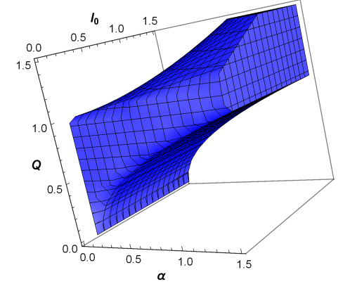
Figure 1: Parameter space for the existence of an HBH.

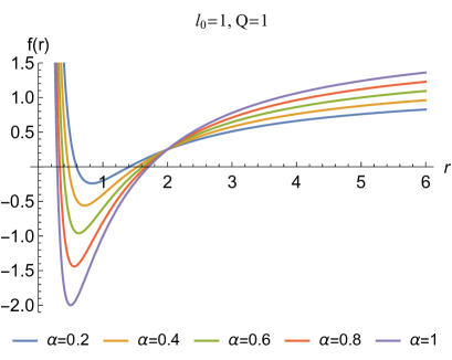
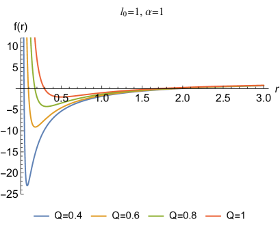
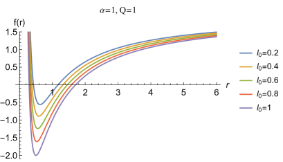
Figure 2: The metric function (5) vs. $r$ for different values of the BH parameters ($M=1$).

For a clear understanding of the parameter region enabling the BH to exist, a graph of the metric function (5) is generated in Fig. 2.

III Spinorial wave equations

The aim of this section is to review Dirac and Rarita-Schwinger equations in the background of the HBH solution.

III.1 Dirac equation

Our focus in this part is on obtaining the effective potential for fermions propagating in HBH geometry with spin- 1/2 field. Hence, we consider the vielbein formalism for the spin- 1/2 fields in curved spacetime (1), the vielbein can be defined as follows

$$e_{\widehat{\alpha}}^{\mu}=daig\left(\frac{1}{\sqrt{g}},\sqrt{g},\frac{1}{r},\frac{1}{r\sin\theta}\right).$$ (8)

The Dirac equation for massive spin-1/2 particles

$$\gamma^{\mu}\left[\left(\partial_{\mu}+\Gamma_{\mu}\right)+m\right]\Psi=0,$$ (9)

where, $\gamma^{\mu}$ is the Dirac gamma matrix and $\Gamma_{\mu}$ is the spin connection, which can be expressed in terms of the Christoffel symbols $\Gamma_{\mu\nu}^{\rho}$ as follows

$$\Gamma_{\mu}=\frac{1}{8}e_{\widehat{\alpha}}^{\rho}\left(\partial_{\mu}e_{\rho\widehat{\beta}}-\Gamma_{\mu\rho}^{\sigma}e_{\sigma\widehat{\beta}}\right)\left[\gamma^{\widehat{\alpha}},\gamma^{\widehat{\beta}}\right].$$ (10)

Here, the Dirac gamma matrices, $\gamma^{\mu}$are represented in terms of the Pauli spin matrices $\sigma^{i}\left(i=0,1,2,3\right).$ The solution procedure of Dirac’s equation (9) will be ignored in this study due to the repetition of references Wong ; badawi2023 . We will present the final answer as a Schrödinger-like one-dimensional wave equation with Dirac field effective potential. Thus, the effective potentials of the massive fermionic waves having spin- 1/2 and moving in the HBH geometry are,

$$V_{\pm 1/2}=\pm\frac{dW}{dr_{\ast}}+W^{2},$$ (11)

where

$$W=\frac{\left(\sqrt{g}/r\right)\sqrt{\lambda^{2}+m^{2}r^{2}}}{1+\left(g/2\omega\right)\left(\lambda m/\left(\lambda^{2}+m^{2}r^{2}\right)\right)},$$ (12)

here, $\lambda=\left(\frac{1}{2}+s\right)$ is the standard spherical harmonics indices, and $\omega$ is the angular frequency of the incoming field. Effective potentials are expressed explicitly as follows:

$$\begin{split}V_{\pm 1/2}=\frac{\left(\lambda^{2}+m^{2}r^{2}\right)^{5/2}\sqrt{g}}{D^{2}}&\Bigg{[}\frac{\sqrt{g}}{r^{2}}\left(\lambda^{2}+m^{2}r^{2}\right)^{1/2}\pm\left(\frac{g^{\prime}}{2r}-\frac{g}{r^{2}}\right)\pm 3m^{2}g\\ &\mp\frac{g}{rD}\left(2m^{2}r+(\lambda m/2\omega)g^{\prime}\right)\Bigg{]},\end{split}$$ (13)

where

$$D=\left(\lambda^{2}+m^{2}r^{2}+\left(\lambda m/2\omega\right)g\right).$$

We can obtain the effective potential of massless Dirac fields (fermions) propagating in this spacetime by setting $m=0$ in (13) namely

$$V_{\pm 1/2}=\frac{\lambda}{r^{2}}\left(\lambda g\pm\frac{r\sqrt{g}g^{\prime}}{2}\mp g^{3/2}\right).$$ (14)

III.2 Rarita-Schwinger equation

We will use the massless form of the Rarita-Schwinger equation to represent the spin- 3/2 field,

$$\gamma^{\mu\nu\alpha}\widetilde{\emph{D}}_{\nu}\psi_{\alpha}=0$$ (15)

where $\widetilde{\emph{D}}_{\nu}$ is the super covariant derivative, $\psi_{\alpha}$ indicates the spin-3/2 field and $\gamma^{\mu\nu\alpha}$ is the antisymmetric of Dirac gamma matrices given by

$$\gamma^{\mu\nu\alpha}=\gamma^{[\mu}\gamma^{\nu}\gamma^{\alpha]}=\gamma^{\mu}\gamma^{\nu}\gamma^{\alpha}-\gamma^{\mu}g^{\nu\alpha}+\gamma^{\nu}g^{\mu\alpha}-\gamma^{\alpha}g^{\mu\nu}.$$ (16)

The super covariant derivative for the spin-3/2 field in our BH spacetime can be written as

$$\widetilde{\emph{D}}_{\nu}=\nabla_{\nu}+\frac{1}{4}\gamma_{\alpha}F_{\nu}^{\alpha}+\frac{i}{8}\gamma_{\nu\alpha\mu}F^{\alpha\mu}.$$ (17)

The solution procedure of Dirac’s equation (15) will be ignored in this study due to the repetition of references chen16 ; chen18 . We will present the final answer as a Schrödinger-like one-dimensional wave equation with Dirac field effective potential. Thus, the explicit forms of the effective potentials for spin-3/2 fermions are written as

$$V_{1,2}=g\frac{\overline{\lambda}\left(1-\overline{\lambda}^{2}\right)}{r\left(g-\overline{\lambda}^{2}\right)}\left[\frac{\overline{\lambda}\left(1-\overline{\lambda}^{2}\right)}{r\left(g-\overline{\lambda}^{2}\right)}\pm\left(\frac{rg^{\prime}-2g}{2r\sqrt{g}}\right)\mp\frac{\sqrt{g}g^{\prime}}{\left(g-\overline{\lambda}^{2}\right)}\right],$$ (18)

where the eigenvalue $\overline{\lambda}=\left(l+1/2\right)$ , and $l=3/2,5/2,7/2,...$.

IV GFs of HBH

When attempting to formulate a general description of the spectrum observed by an observer at infinity, it is critical to know the transmission amplitude of the BH’s radiation or GFs hb20 ; hb21 ; hb22 ; hb23 ; hb24 ; hb25 ; hb26 ; hb27 ; hb28 ; hb29 ; hb30 . Our aim of this section is to examine the GFs of HBH using the rigorous bounds and general semi-analytic bounds. Consequently, it is possible to determine how the potential affects the GF. The transmission probability $\sigma_{l}\left(w\right)$ is given by hb29 ; hb30

$$\sigma_{l}\left(w\right)\geq\sec h^{2}\left(\int_{-\infty}^{+\infty}\wp dr_{\ast}\right),$$ (19)

in which $r_{\ast}$ is the tortoise coordinate and

$$\wp=\frac{1}{2h}\sqrt{\left(\frac{dh\left(r_{\ast}\right)}{dr_{\ast}}\right)^{2}+(w^{2}-V_{eff}-h^{2}\left(r_{\ast}\right))^{2}}.$$ (20)

where $h(r_{\ast})$ is a positive function satisfying $h\left(-\infty\right)=h\left(+\infty\right)=w$. For more details, one can see hb29 . We select $h=w$. Therefore, Eq. (20)

$$\sigma_{l}\left(w\right)\geq\sec h^{2}\left(\int_{r_{h}}^{+\infty}\frac{V_{eff}}{2w}dr_{\ast}\right).$$ (21)

In this process, the metric function plays a significant role in determining the relationship between the GFs and the effective potential. Our GF calculations will be carried out in three cases since we have fermions with different spins. When computing GFs, we usually focus on the study of the potential $V_{+}$.

IV.1 Spin- 1/2 fermions emission

In this section, we will look at the GF using rigorous bounds. This method allows us to analyze the results qualitatively. As a result, the potential’s effect on the greybody factor can be calculated. The rigorous bounds on the greybody factors are given by

$$\sigma_{l}\left(w\right)\geq\sec h^{2}\left(\int_{-\infty}^{+\infty}\left|\frac{V_{eff}}{2w}\right|dr_{\ast}\right)$$ (22)

Substituting the effective potential (11) derived from Dirac equations into Eq. (22), we obtain

$$\sigma_{l}^{+}\left(w\right)\geq\sec h^{2}\left[\frac{1}{2w}\left(\int_{-\infty}^{+\infty}\left|\frac{dW}{dr_{\ast}}\right|dr_{\ast}+\int_{-\infty}^{+\infty}\left|W^{2}\right|dr_{\ast}\right)\right].$$ (23)

We will discuss separately the first and second integrals in Eq. (23). For the first integral, we have

$$\int_{-\infty}^{+\infty}\left|\pm\frac{dW}{dr_{\ast}}\right|dr_{\ast}=W\left|{}_{r_{+}}^{r_{-}}=\right.0,$$ (24)

where $r_{+}$ and $r_{-}$ are the two horizons (6) of the BH. The second integral can be written as

$$\int_{r_{+}}^{r-}\left(\frac{\left(\lambda^{2}+m^{2}r^{2}\right)^{2}}{r^{2}\left[(\lambda m/2k)\left|g\right|+\left(\lambda^{2}+m^{2}r^{2}\right)\right]}\right)dr,$$ (25)

There is a considerable difference between the results of this formulation for massless and massive instances. These two cases are, therefore, considered separately.

IV.1.1 Massless case

To compute the GFs for massless spin- 1/2 fermions emission, we choose $m=0,$ then the integral (25) becomes

$$\int_{r_{+}}^{r-}\frac{\lambda^{2}}{r^{2}}dr=\lambda^{2}\left(\frac{1}{r_{+}}-\frac{1}{r_{-}}\right).$$ (26)

Substituting the result of this integral in Eq. (23), the rigorous bound can be expressed as

$$\sigma_{l}^{+}\left(w\right)\geq\sec h^{2}\left(\frac{\lambda^{2}}{2\omega}\left[\frac{1}{r_{+}}-\frac{1}{r_{-}}\right]\right).$$ (27)

After putting the values of the horizons (6), the rigorous bound of the HBH for massless fermions is calculated as follows:

$$\sigma_{l}^{+}\left(w\right)\geq\sec h^{2}\left(\frac{\lambda^{2}}{2\omega}\left[\frac{-\sqrt{\left(2M+\alpha M+\alpha l_{0}\right)^{2}-4\left(1+\alpha\right)Q^{2}}}{Q^{2}}\right]\right).$$ (28)

A massless spin- $1/2$ fermion bound in an HBH exhibits a behavior that depends on the distance between two horizons, as reflected in the argument of function $sech$. It is, therefore, possible to analyze the behavior of the bound by considering how the distance between two horizons varies with the hairy parameters. These can be illustrated in Figs. 3, 4, 5 and 6.

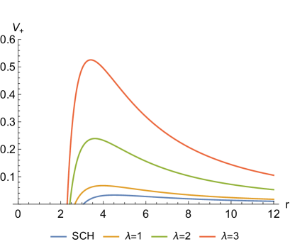
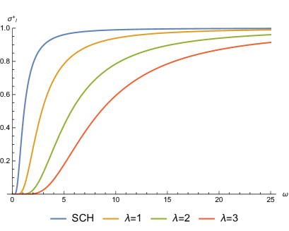
Figure 3: The left panel shows the potential (14) for massless spin- $1/2$ field with $M=1$, $\alpha=0.5$, $l_{0}=1$ and $Q=0.7$. The right panel shows the corresponding GF bound.

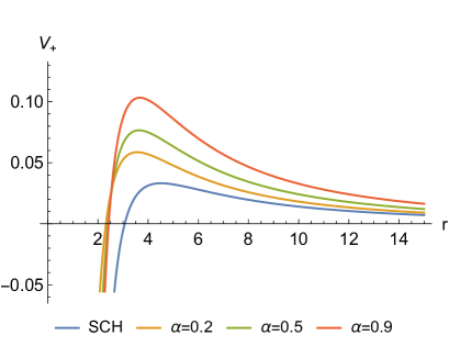
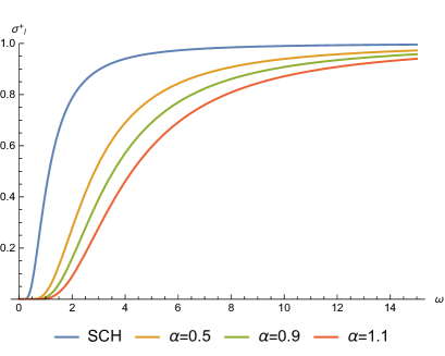
Figure 4: The left panel shows the potential (14) for massless spin- $1/2$ field with $M=1$, $\lambda=1$, $l_{0}=1$ and $Q=0.6$. The right panel shows the corresponding GF bound.

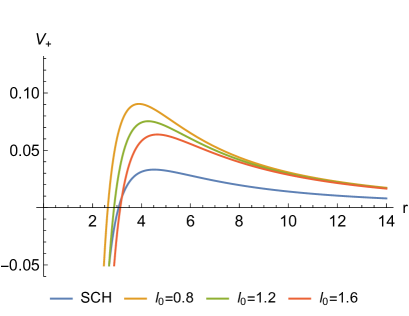
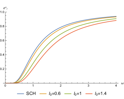
Figure 5: The left panel shows the potential (14) for massless spin- $1/2$ field with M = 1, $\lambda=1$, $\alpha=0.8$ and $Q=0.4$. The right panel shows the corresponding GF bound.

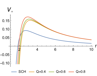
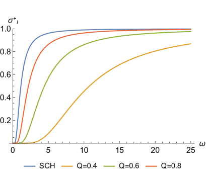
Figure 6: The left panel shows the potential (14) for massless spin- $1/2$ field with $M=1$, $\lambda=1$, $\alpha=1$ and $l_{0}=1.4$. The right panel shows the corresponding GF bound.

Using the potential shape as a starting point, we can examine how the rigorous bound $\sigma_{l}$ behaves. This can be achieved by varying the hairy parameters, $(\alpha,Q,l_{0})$ and angular parameter $\lambda$. By adjusting the hairy parameters, the potential increases when $\lambda$ increases, as shown in the left panel of Fig. 3. As shown in the right panel of Fig. 3, the GF decreases for a given value of $\omega$ because the wave is more difficult to transmit through the higher potential. Similar analysis can be performed for the hairy parameters $(\alpha$ and $l_{0})$, as shown in Figs. 4 and 5. The analysis for the hairy parameter $Q$, on the other hand, is the inverse, as shown in Fig. 6.

IV.1.2 Massive case

To compute the GFs for massive spin- 1/2 fermions emission, we will write the integral (25) as

$$\int_{r_{+}}^{r-}\frac{\lambda^{2}\left(1+\mu^{2}r^{2}\right)}{r^{2}\left(1+\frac{\mu g}{\left(1+\mu^{2}r^{2}\right)2w}\right)}dr=\int_{r_{+}}^{r-}Adr,$$ (29)

where

$$A=\frac{\lambda^{2}\left(1+\mu^{2}r^{2}\right)}{r^{2}\left(1+\frac{\mu g}{\left(1+\mu^{2}r^{2}\right)2w}\right)},\hskip 28.45274pt\mu=m/\lambda.$$ (30)

When we consider the equation above, we can see that $A$ is larger than $1$, since the factor $1+\frac{\mu g}{\left(1+\mu^{2}r^{2}\right)2w}>1$. In this way, we can approximate the integrand, which is given by the following

$$A=\frac{\lambda^{2}\left(1+\mu^{2}r^{2}\right)}{r^{2}\left(1+\frac{\mu g}{\left(1+\mu^{2}r^{2}\right)2w}\right)}\leq\frac{\lambda^{2}}{r^{2}}\left(1+\mu^{2}r^{2}\right)=A_{app}.$$ (31)

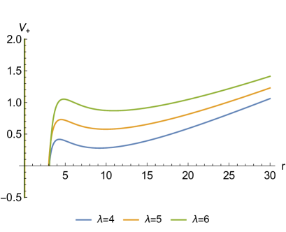
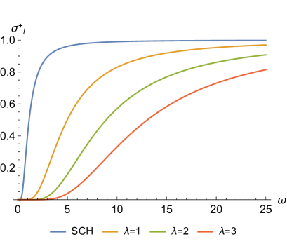
Figure 7: The left panel shows the potential (13) for massive spin- 1/2 field with $M=1$, $m=0.5$, $Q=0.7$ and $l_{0}=0.5$. The right panel shows the corresponding GF bound

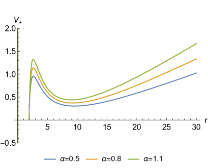
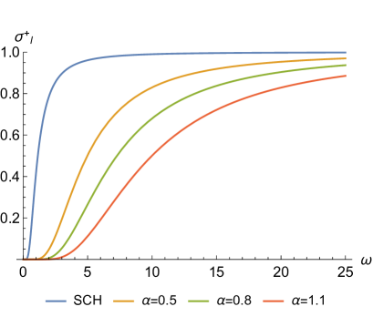
Figure 8: The left panel shows the potential (13) for massive spin- 1/2 field for varying $Q$ with $M=1$, $m=1$, $\alpha=0.4$ and $l_{0}=1$. The right panel shows the corresponding GF bound

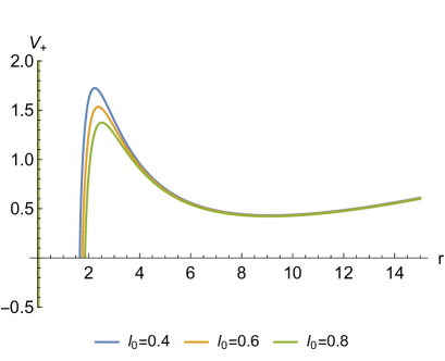
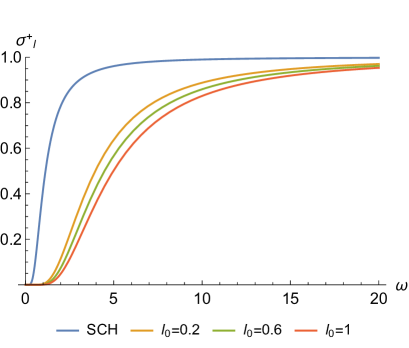
Figure 9: The left panel shows the potential (13) for massive spin- 1/2 field with $M=1$, $m=1$, $Q=0.4$ and $\alpha=1$. The right panel shows the GFs of massive spin- $1/2$ field for varying $l_{0}$

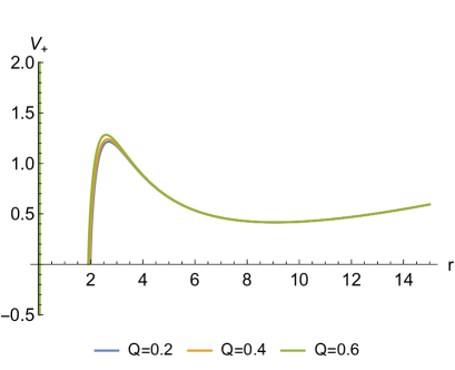
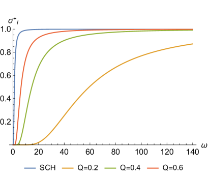
Figure 10: The left panel shows the potential (13) for massive spin- 1/2 field with $M=1$, $m=1$, $l_{0}=1$ and $\alpha=1$. The right panel shows the GFs of massive spin- $1/2$ field for varying $Q$

The integral Eq. (29) can be evaluated by using the same arguments as in hb33 namely,

$$\sigma_{l}^{+}\left(w\right)\geq\sec h^{2}\left(\int_{r_{+}}^{r-}A_{app}dr\right)$$ (32)

$$\sigma_{l}^{+}\left(w\right)\geq\sec h^{2}\left(\frac{\lambda^{2}}{2\omega}\left[\frac{r_{-}-r_{+}}{r_{+}r_{-}}\left(1+\mu^{2}r_{+}r_{-}\right)\right]\right).$$ (33)

After putting the values of the horizons in Eq. (33), the rigorous bound of the HBH for massive fermions is calculated as follows

$$\sigma_{l}^{+}\left(w\right)\geq\sec h^{2}\left(\frac{\lambda^{2}}{2\omega}\left[\frac{-\sqrt{\left(2M+\alpha M+\alpha l_{0}\right)^{2}-4\left(1+\alpha\right)Q^{2}}}{\left(1+\alpha\right)Q^{2}}\left(1+\alpha+\mu^{2}Q^{2}\right)\right]\right).$$ (34)

This expression is reduced to that of the GF bound for the massless case when $\mu\rightarrow 0.$ According to (34), the bound for the massive case is still reliant on the hairy parameters in the same way that the bound for the massless case is. The GF bounds for massive spin- $1/2$ are illustrated in Figs. 7- 10. It is worth to mention that according to Ref olliv , HBHs were created by demanding that they satisfy the strong energy condition or dominant energy condition between the BH’s horizon $r\geq 2M$ and infinity. As shown in olliv , all of the new HBHs solutions correspond to Schwarzschild vacuum deformations. Therefore, the plots of the effective potential exhibits a negative gap when the $r$ coordinate is less than the horizon as shown in the left panel of the Figs. 7- 10.

IV.2 Spin- 3/2 fermions emission

With general semi-analytic bounds, we can obtain the GF for spin-3/2 fermions emission using the potential derived in (18). Then, Eq. (21) becomes

$$\begin{split}\sigma_{l}\left(w\right)\geq\sec h^{2}&\Bigg{[}\frac{\lambda}{2\omega}\int_{r_{h}}^{+\infty}\Bigg{(}\frac{\overline{\lambda}\left(1-\overline{\lambda}^{2}\right)}{r^{2}\left(g-\overline{\lambda}^{2}\right)^{2}}\\ &\left(\overline{\lambda}\left(1-\overline{\lambda}^{2}\right)+\frac{\left(rg^{\prime}-2g\right)\left(g-\overline{\lambda}^{2}\right)}{2\sqrt{g}}-r\sqrt{g}g\right)dr\Bigg{)}\Bigg{]},\end{split}$$ (35)

We will apply asymptotic series expansion to overcome the difficulties encountered in evaluating the above complicated integral (35). Then, the GF of massless spin- $3/2$ fermions is

$$\begin{split}\sigma_{l}^{+}\left(w\right)\geq\sec h^{2}&\Bigg{[}\frac{1}{2w}\Bigg{(}\frac{\overline{\lambda}\left(1-\overline{\lambda}^{2}\right)\left(2\alpha+\alpha^{2}+\left(2\overline{\lambda}\sqrt{1+\alpha}-1-\overline{\lambda}^{2}\right)\right)\left(2M+\alpha\left(l_{0}+M\right)\right)}{2\overline{\lambda}\sqrt{1+\alpha}\left(1+\alpha-\overline{\lambda}^{2}\right)r_{h}^{2}}\\ &+\frac{\overline{\lambda}\left(1-\overline{\lambda}^{2}\right)\left(\alpha\sqrt{1+\alpha}-\left(\sqrt{1+\alpha}-\overline{\lambda}\right)\left(\overline{\lambda}^{2}-1\right)\right)}{\left(1+\alpha-\overline{\lambda}^{2}\right)r_{h}}\Bigg{)}\Bigg{]},\end{split}$$ (36)

Figure 11 shows the variation of the GF of massless spin-$3/2$ field with various hairy parameters. The graph shows that as $\alpha$ parameter increases, GF decreases, whereas GF increases as $l_{0}$ increases.

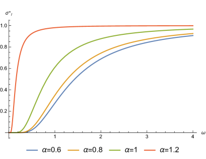
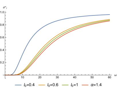
Figure 11: The GFs of massless spin- $3/2$ field for varying $\alpha$ (left panel) and $l_{0}$ (right panel) with $M=1$, $m=0.5$, $Q=0.7$ and $l_{0}=0.5$.

V Ringdown waveform

With the help of the time domain integration method gundlach1 , we, in this section, intend to scrutinize the impact of parameters $(\alpha$,$Q,l_{0})$ on the time evolution of the massless fermionic spin -1/2 and spin -3/2 fields. We implement the time domain integration method with initial conditions $\psi(r_{*},t)=\exp\left[-\dfrac{(r_{*}-\hat{r}_{*})^{2}}{2\sigma^{2}}\right]$ and $\psi(r_{*},t)|_{t<0}=0$. We choose the values of $\Delta t$ and $\Delta r_{*}$ such that the Von Neumann stability condition, $\frac{\Delta t}{\Delta r_{*}}<1$, is satisfied. The time profile helps us scrutinize the qualitative variation of the decay rate and the frequency with the variation of parameters $\alpha$,$Q,l_{0}$.

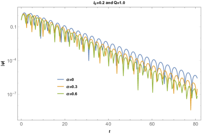
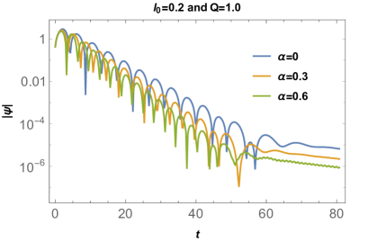
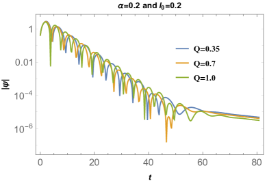
Figure 12: Time profile of massless fermionic spin -1/2 perturbation. Here, we have taken $\lambda=3$.

In Fig. 12, we show the ringdown waveform for a massless spin -$1/2$ perturbation field, and in Fig. 13, we provide the waveform for a massless spin -$3/2$ field. From Figs 12, 13, we observe that the decay rate as well the frequency increases with an increase in $\alpha$ for both the perturbations. The parameter $l_{0}$ influences quasinormal modes in such a way that the decay rate, as well as the frequency, first decreases and then increases with an increase in $l_{0}$. The impact of $Q$ can be inferred from Figs. 12, 13. We can conclude that the decay rate decreases and the frequency increases with $Q$.

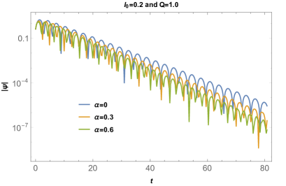
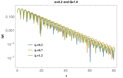
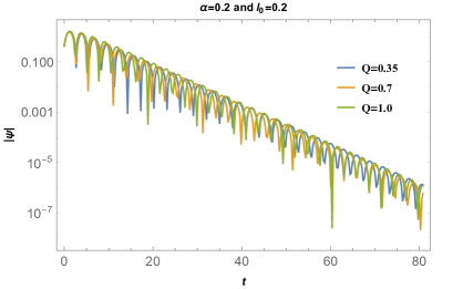
Figure 13: Time profile of massless fermionic spin- 3/2 perturbation. Here, we have taken $\overline{\lambda}=3$.

To compare the ringdown waveforms of massless and massive spin -1/2 perturbations, we plot them for massless and massive perturbations in Fig. 14. It clearly shows that the frequency and decay rate for massive perturbation is less than those for massless perturbation.

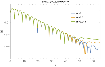
Figure 14: Time profile of massless and massive fermionic spin- 1/2 perturbations. Here, we have taken $\lambda=2$.

Our study in this section conclusively illustrates the impact of parameters $(\alpha,Q,l_{0})$ on the time evolution of perturbation fields and enriches our understanding of this very important aspect of BH physics.

VI Hawking spectra and sparsity

The Hawking spectra and the sparsity of radiation emitted by HBH are investigated in this section. The power emitted per unit frequency in the $l^{th}$ mode is yg2017 ; fg2016

$$P_{l}\left(\omega\right)=\frac{A}{8\pi^{2}}\sigma_{l}^{+}\frac{\omega^{3}}{e^{\omega/T_{H}}-1},$$ (37)

where A is taken to be the horizon area yg2017 . $T_{H}$ is the Hawking temperature given by

$$T_{H} = \frac{1}{4\pi}\frac{dg}{dr}|_{r=r_{+}}$$

$$= \frac{H1}{H2}\quad\text{where}$$

$$H1 = (\alpha+1)^{2}\left(\alpha^{2}\left(l_{0}+M\right){}^{2}+2M\left(\sqrt{\left(\alpha\left(l_{0}+M\right)+2M\right){}^{2}-4(\alpha+1)Q^{2}}+2M\right)\right.$$

$$\left.+\alpha\left(l_{0}+M\right)\left(\sqrt{\left(\alpha\left(l_{0}+M\right)+2M\right){}^{2}-4(\alpha+1)Q^{2}}+4M\right)-4\alpha Q^{2}-4Q^{2}\right),$$

$$H2 = \pi\left(\alpha\left(l_{0}+M\right)+\sqrt{\left(\alpha l_{0}+(\alpha+2)M\right){}^{2}-4(\alpha+1)Q^{2}}+2M\right){}^{3}.$$

The total power emitted in the $l^{th}$ mode is given by

$$P_{tot}=\int_{0}^{\infty}P_{\l}\left(\omega\right)d\omega.$$ (39)

Combining Eqs. (37, VI) we analyze the qualitative variation of $P_{l}$ with respect to $\omega$ for different scenarios in Figs. 15, 16. From Fig. 15 we observe that the total power emitted by the BH increases with $\alpha$, and the position of the peak shifts towards the right. Figs. 15, 15 also reveal that the total emitted power decreases with $l_{0}$ but increases with $Q$, whereas the peak of the spectrum shifts towards the right for an increase in $l_{0}$ and towards the left for an increase in $Q$. These observations are for a massive fermionic spin -$1/2$ field. Now, for a massless spin -$3/2$ field, we turn our attention towards Fig. 16. From Fig. 16, we observe that the peak of the power spectrum first increases with $\alpha$ and then decreases, whereas the position of the peak always shifts to the right. It is also observed that the total power emitted by the BH increases with $\alpha$. It is evident from Figs. 16, 16 that the total power emitted by the BH increases with $l_{0}$ and decreases with $Q$.

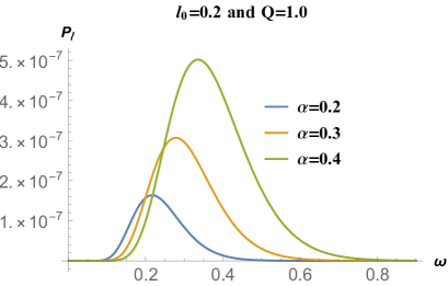
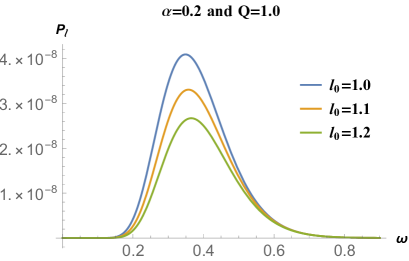
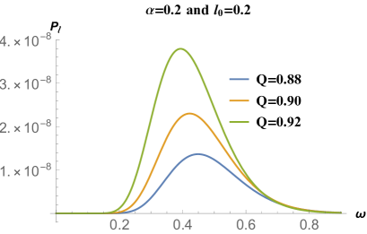
Figure 15: Power spectrum of massive fermionic spin -1/2 field. Here, we have taken $\lambda=2$ and $\mu=0.25$.

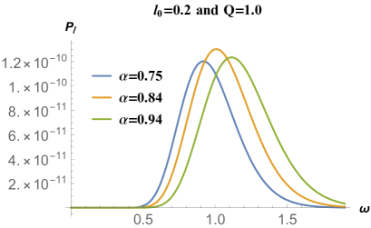
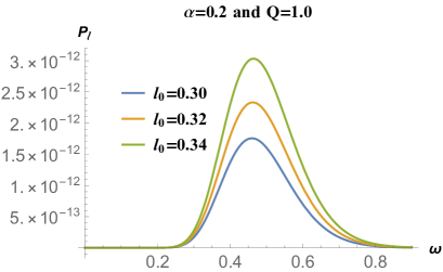
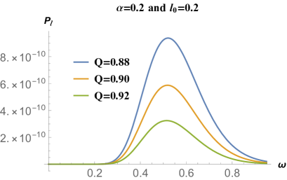
Figure 16: Power spectrum of massless fermionic spin -3/2 field. Here, we have taken $\overline{\lambda}=2$.

To have a quantitative measure of the radiation emitted by the BH, we introduce sparsity, a dimensionless quantity, defined as yg2017 ; fg2016 ; ac2020 ; sh2016 ; sh2015

$$\eta=\frac{\tau_{gap}}{\tau_{emission}}.$$ (40)

Here, $\tau_{gap}$ and $\tau_{emission}$ are the time that is taken by a radiation quantum for emissions and the average time gap between two successive radiation quanta, respectively. These are defined by

$$\tau_{gap}=\frac{\omega_{max}}{P_{tot}}\quad\tau_{emission}\geq\tau_{localisation}=\frac{2\pi}{\omega_{max}},.$$ (41)

where $\tau_{localisation}$ is the time period of the emitted wave of frequency $\omega_{max}$. For $\eta\ll 1$, we will have a continuous flow of Hawking radiation, whereas a large value of $\eta$ implies a sparse Hawking radiation. Quantitative values of $\omega_{max}$, $P_{max}$, $P_{tot}$, and $\eta$ are given in Tables 1, 2, 3 for a massive spin -$1/2$ field and in Tables 4, 5, 6 for a massless spin -$3/2$ field. These tables reinforce our conclusions drawn from Figs.15, 16. Additionally, we can also observe the effect of various parameters on the sparsity. From Tables 1, 2, 3 we see that the sparsity of the radiation decreases with $\alpha$ and $Q$ but increases with $l_{0}$ for a massive spin -$1/2$ field. It can be observed from the Table 4 that the sparsity initially decreases and then increases with $\alpha$ having critical value at $\alpha=0.871$. On the other hand, $\eta$ decreases with $l_{0}$ and increases with $Q$ as evident from Tables 5, 6.

Table 1: Numerical values of $\omega_{max}$, $P_{max}$, $P_{tot}$, and $\eta$ for massive spin -1/2 perturbation for various values of $\alpha$ with $l_{0}=0.2$, $Q=1$, $\lambda=2$, and $\mu=0.25$.

$\alpha$	0.2	0.4	0.6	0.8	1.0
$\omega_{\max}$	0.217541	0.335618	0.445538	0.552871	0.656921
$P_{max}$	$1.63372$ $\times$ $10^{-7}$	$5.0177$ $\times$ $10^{-7}$	$1.0799$ $\times$ $10^{-6}$	$1.96344$ $\times$ $10^{-6}$	$3.21797$ $\times$ $10^{-6}$
$P_{\text{tot}}$	$2.58744\times 10^{-8}$	$1.22075\times 10^{-7}$	$3.47708\times 10^{-7}$	$7.82162\times 10^{-7}$	$1.524\times 10^{-6}$
$\eta$	$2.91094\times 10^{5}$	$1.46853\times 10^{5}$	$9.08604\times 10^{4}$	$6.21972\times 10^{4}$	$4.50672\times 10^{4}$

Table 2: Numerical values of $\omega_{max}$, $P_{max}$, $P_{tot}$, and $\eta$ for massive spin -1/2 perturbation for various values of $l_{0}$ with $\alpha=0.2$, $Q=1$, $\lambda=2$ and $\mu=0.25$.

$l_{0}$	$0.2$	$0.4$	$0.6$	$0.8$	$1.0$
$\omega_{\max}$	$0.217541$	$0.268992$	$0.304746$	$0.331781$	$0.359994$
$P_{max}$	$1.63372\times 10^{-7}$	$1.32654\times 10^{-7}$	$9.29835\times 10^{-8}$	$6.21794\times 10^{-8}$	$4.05768\times 10^{-8}$
$P_{\text{tot}}$	$2.58744\times 10^{-8}$	$2.51919\times 10^{-8}$	$1.94188\times 10^{-8}$	$1.37758\times 10^{-8}$	$9.41305\times 10^{-9}$
$\eta$	$2.91094\times 10^{5}$	$4.57127\times 10^{5}$	$7.61159\times 10^{5}$	$1.27176\times 10^{6}$	$2.19119\times 10^{6}$

Table 3: Numerical values of $\omega_{max}$, $P_{max}$, $P_{tot}$, and $\eta$ for massive spin -1/2 perturbation for various values of $Q$ with $\alpha=0.2$, $l_{0}=0.2$, $\lambda=2$ and $\mu=0.25$.

$Q$	$0.35$	$0.48$	$0.61$	$0.74$	$0.87$
$\omega_{\max}$	$1.38934$	$0.9631$	$0.862479$	$0.599048$	$0.436239$
$P_{\max}$	$1.65373\times 10^{-22}$	$2.06223\times 10^{-16}$	$6.96079\times 10^{-13}$	$1.84607\times 10^{-10}$	$1.0156\times 10^{-8}$
$P_{\text{tot}}$	$8.17937\times 10^{-23}$	$9.30337\times 10^{-17}$	$2.95924\times 10^{-13}$	$6.21224\times 10^{-11}$	$2.96887\times 10^{-9}$
$\eta$	$3.75593\times 10^{21}$	$1.5868\times 10^{15}$	$4.00071\times 10^{11}$	$9.19382\times 10^{8}$	$1.02018\times 10^{7}$

Table 4: Numerical values of $\omega_{max}$, $P_{max}$, $P_{tot}$, and $\eta$ for massless spin -3/2 perturbation for various values of $\alpha$ with $l_{0}=0.2$, $Q=1$, $\overline{\lambda}=2$.

$\alpha$	$0.2$	$0.4$	$0.6$	$0.8$	$1.0$
$\omega_{\max}$	$0.436239$	$0.599048$	$0.862479$	$0.9631$	$1.12591$
$P_{\max}$	$2.75106\times 10^{-13}$	$1.56319\times 10^{-11}$	$6.72487\times 10^{-11}$	$1.27798\times 10^{-10}$	$1.09201\times 10^{-10}$
$P_{\text{tot}}$	$5.93889\times 10^{-14}$	$4.91794\times 10^{-12}$	$3.09834\times 10^{-11}$	$6.46398\times 10^{-11}$	$6.82237\times 10^{-11}$
$\eta$	$5.09993\times 10^{11}$	$1.16134\times 10^{10}$	$3.82109\times 10^{9}$	$2.28383\times 10^{9}$	$2.95727\times 10^{9}$

Table 5: Numerical values of $\omega_{max}$, $P_{max}$, $P_{tot}$, and $\eta$ for massless spin -3/2 perturbation for various values of $l_{0}$ with $\alpha=0.2$, $Q=1$, $\overline{\lambda}=2$.

$l_{0}$	$0.2$	$0.4$	$0.6$	$0.8$	$1.0$
$\omega_{\max}$	$0.436239$	$0.436239$	$0.436239$	$0.436239$	$0.436239$
$P_{\max}$	$2.75106\times 10^{-13}$	$5.64809\times 10^{-12}$	$2.68204\times 10^{-11}$	$7.27206\times 10^{-11}$	$1.47412\times 10^{-10}$
$P_{\text{tot}}$	$5.93889\times 10^{-14}$	$1.45152\times 10^{-12}$	$7.46322\times 10^{-12}$	$2.07892\times 10^{-11}$	$4.21614\times 10^{-11}$
$\eta$	$5.09993\times 10^{11}$	$2.08664\times 10^{10}$	$4.0583\times 10^{9}$	$1.45691\times 10^{9}$	$7.18382\times 10^{8}$

Table 6: Numerical values of $\omega_{max}$, $P_{max}$, $P_{tot}$, and $\eta$ for massless spin -3/2 perturbation for various values of $Q$ with $\alpha=0.2$, $l_{0}=0.2$, $\overline{\lambda}=2$.

$Q$	$0.35$	$0.48$	$0.61$	$0.74$	$0.87$
$\omega_{\max}$	$0.536861$	$0.536861$	$0.536861$	$0.536861$	$0.536861$
$P_{\max}$	$1.86991\times 10^{-8}$	$1.50416\times 10^{-8}$	$1.03636\times 10^{-8}$	$5.23738\times 10^{-9}$	$1.13655\times 10^{-9}$
$P_{\text{tot}}$	$6.08023\times 10^{-9}$	$4.85163\times 10^{-9}$	$3.30778\times 10^{-9}$	$1.64503\times 10^{-9}$	$3.43338\times 10^{-10}$
$\eta$	$7.54438\times 10^{6}$	$9.45489\times 10^{6}$	$1.38678\times 10^{7}$	$2.78849\times 10^{7}$	$1.33605\times 10^{8}$

VII Conclusion

We begin the assessment of how the rigorous bound $\sigma_{l}$ behaves, comprehending the potential shape of the potential associated with fulminic perturbation. The shape of the potential depends crucially on the hairy parameters, $(\alpha,Q,l_{0}$), as well as on the angular parameter $\lambda$. According to the findings, the left panel of Fig. 3 displays that the potential rises with the increase in the parameter $\lambda$ for particular hairy parameters. The right panel of Fig. 3, however, shows that the GF decreases with $\lambda$ for a given value of $\omega$ because the wave is more difficult to transmit through the higher potential. Similar analysis follows for the hairy parameters $(\alpha$ and $l_{0})$ as it is transparent from the Figs. 4 and 5. Fig. 6 displays that the action of the hairy parameter $Q$, on the other hand, is entirely the inverse of what was found for the parameter $(\alpha$ and $l_{0})$.

Using the argument hb33 leads us to find out the GFs bounds for both massive and massless cases. As per (34), the massive case’s bound depends on the hairy parameters, just as the bound for the massless case. The GFs bounds for massive spin- $1/2$ fermion are depicted in Figs. 7- 10. Along with the spin- $1/2$ fermion, we have considered the spin-$3/2$ fermion in our study, where Dirac equation is replaced by the Schwinger-Dyson equation. Fig. (11) shows the variation of the GF of massless spin-$3/2$ fermion with various hairy parameters. The graph indicates that while GF increases as $l_{0}$ increases, it drops as $\alpha$ parameter increases.

Our study includes the ringdown waveform due to the perturbation of massless spin -$1/2$ and spin -$3/2$ fields. Fig. 12 displays the ringdown waveform for a massless spin -$1/2$ The perturbation field in which Fig. 13 displays the same due to the perturbation of spin -$3/2$ field. From Figs. (12, 13) we observe that the decay rate, as well as the frequency, increases with an increase in $\alpha$ for both the perturbations caused by both of the fields having the odd integral spin $1/2$ and $3/2$. The influences of the parameter $l_{0}$ on the quasinormal modes are as follows. Both the decay rate and the frequency of oscillation decrease, to begin with, and then increase with an increase in $l_{0}$. The impact of $Q$ can be inferred from Figs. (12, 13). It is found that the decay rate decreases, whereas the frequency increases when the value of $Q$ enhances.

When the study of the emissive power of Hawking radiation is carried out, we analyze the qualitative variation of $P_{l}$ with respect to $\omega$ for different scenarios in Figs. 15, 16. Combining Eqs. (37, VI) we became able to study the qualitative behavior of the variation of $P_{l}$ with respect to $\omega$. According to Fig. 15, the overall power emission rises with $\alpha$, and the location of the peak of the spectra moves to the right. Figs. (15, 15) reveal that the total emitted power decreases with $l_{0}$ but increases with $Q$, whereas the peak of the spectra acquire a right shift and left shift, respectively, for an increase in $l_{0}$ and $Q$. These findings pertain to the perturbation when it is caused due to the massive fermionic field having spin -$1/2$. For the perturbation due to the massless spin -$3/2$ fermionic field, let us focus on Fig. 16. Fig. 16 shows that the peak of the power spectrum increases with $\alpha$, to begin with, and then is followed by a drop, whereas the position of the peak of the spectra always shifts to the right. It is also observed that the total power emitted by the BH increases with $\alpha$. The Figs. 16, and 16 exhibit that the total power emitted by the BH enhances with $l_{0}$; however, it drops off with Q.

For a quantitative idea, we compute the numerical values of $\omega_{max}$, $P_{max}$, $P_{tot}$, and $\eta$ which are displayed in Tables 1, 2, and 3 for a massive spin -$1/2$ fermionic field, and for a massless spin -$3/2$ field, the corresponding quantities are presented in Tables 4, 5, and 6. These tables reinforce our conclusions drawn from Figs.15, and 16. Additionally, we can observe the effect of various parameters on the sparsity of the Hawking radiation. From Tables 1, 2, and 3, we see that the sparsity of the radiation expands with $\alpha$ and $Q$ but shrinks with $l_{0}$ for a massive spin -$1/2$ field. Table 4 furnishes that the sparsity initially diminishes and then enhances with $\alpha$. Conversely, $\eta$ falls off with $l_{0}$ and grows with $Q$ according to the numerical information of the Tables 5 and 6. According to our study, hairy parameters have significant effects on GFs, QNMs, Hawking spectra, and sparsity. These findings will enhance our understanding of hairy black holes and their astrophysical significance.
Acknowledgements
We are thankful to the Editor and anonymous Referees for their constructive suggestions and comments.

Data Availability
No data availability in this manuscript.

References

- (1) S. W. Hawking, Commun. Math. Phys. 25 (1972) 15215
- (2) S. W. Hawking, M. J. Perry and A. Strominger, Phys. Rev. Lett. 116 (2016) 231301 [arXiv:1601.00921 [hep-th]].
- (3) T. P. Sotiriou and V. Faraoni, Phys. Rev. Lett. 108 (2012) 081103 [arXiv:1109.6324 [gr-qc]].
- (4) E. Babichev and C. Charmousis, JHEP 1408 (2014) 106 [arXiv:1312.3204 [gr-qc]].
- (5) T. P. Sotiriou and S. Y. Zhou, Phys. Rev. Lett. 112 (2014) 251102 [arXiv:1312.3622 [gr-qc]].
- (6) C. A. R. Herdeiro and E. Radu, Int. J. Mod. Phys. D 24 (2015) 1542014 [arXiv:1504.08209 [gr-qc]].
- (7) P. Canate, L. G. Jaime and M. Salgado, Class. Quant. Grav. 33 (2016) 155005 [arXiv:1509.01664 [gr-qc]].
- (8) R. Benkel, T. P. Sotiriou and H. Witek, Class. Quant. Grav. 34 (2017) no.6, 064001 [arXiv:1610.09168 [gr-qc]].
- (9) G. Antoniou, A. Bakopoulos and P. Kanti, ”Evasion of No-Hair Theorems in Gauss-Bonnet Theories,” arXiv:1711.03390 [hep-th].
- (10) A. Anabalon, A. Cisterna and J. Oliva, Phys. Rev. D 89, 084050 (2014) [arXiv:1312.3597 [gr-qc]].
- (11) A. Cisterna and C. Erices, Phys. Rev. D 89, 084038 (2014) [arXiv:1401.4479 [gr-qc]].
- (12) A. Cisterna, M. Hassaine, J. Oliva and M. Rinaldi, Phys. Rev. D 96, no. 12, 124033 (2017) [arXiv:1708.07194 [hep-th]].
- (13) M. S. Volkov and D. V. Galtsov, JETP Lett. 50 (1989) 346 [Pisma Zh. Eksp. Teor. Fiz. 50 (1989) 312].
- (14) P. Kanti, N. E. Mavromatos, J. Rizos, K. Tamvakis and E. Winstanley, Phys. Rev. D 54 (1996) 5049 [hep-th/9511071].
- (15) P. Kanti, N. E. Mavromatos, J. Rizos, K. Tamvakis and E. Winstanley, Phys. Rev. D 57 (1998) 6255 [hep-th/9703192].
- (16) M. S. Volkov and D. V. Galtsov, Phys. Rept. 319 (1999) 1 [hep-th/9810070].
- (17) C. Martinez, R. Troncoso, J. Zanelli, Phys.Rev. D 70 (2004) 084035 arXiv:hep-th/0406111
- (18) K. G. Zloshchastiev, Phys. Rev. Lett. 94 (2005) 121101 [hep-th/0408163].
- (19) J. Ovalle, R. Casadio, E. Contreras, and A. Sotomayor, Phys. Dark Univ. 31, 100744 (2021), arXiv:2006.06735 [gr-qc]
- (20) T. P. Sotiriou, Class. Quant. Grav. 32 (2015) 214002 [arXiv:1505.00248 [gr-qc]].
- (21) J. Ovalle, Phys. Lett. B788, 213 (2019), arXiv:1812.03000 [gr-qc].
- (22) J. Ovalle, Phys. Rev. D95, 104019 (2017), arXiv:1704.05899 [gr-qc].
- (23) H. T. Cho, A. S. Cornell, Jason Doukas, and Wade Naylor Phys. Rev. D 75, 104005 (2007).
- (24) Ahmad Al-Badawi and Amani Kraishan, Annals of Physics 458 (2023) 169467.
- (25) Ahmad Al-Badawi and Amani Kraishan, Chinese Journal of Physics, 87 59–69 (2024).
- (26) J. Ovalle, Mod. Phys. Lett. A23, 3247 (2008), arXiv:grqc/0703095 [gr-qc].
- (27) J. Ovalle and R. Casadio, Buy Beyond Einstein Gravity: The Minimal Geometric Deformation Approach in the Brane-World, Springer, 2020
- (28) R. Konoplya and A. Zhidenko, Phys. Lett. B 756, 350 (2016).
- (29) R. Konoplya and A. Zhidenko, Phys. Lett. B 756, 350 (2016) [arXiv:1602.04738 [gr-qc]]; JCAP 1612, no. 12, 043 (2016) [arXiv:1606.00517 [gr-qc]];
- (30) N. Yunes, K. Yagi and F. Pretorius, Phys. Rev. D 94, no. 8, 084002 (2016) [arXiv:1603.08955 [gr-qc]].
- (31) R. A. Konoplya and A. Zhidenko, Rev. Mod. Phys. 83, 793 (2011) [arXiv:1102.4014 [gr-qc]];
- (32) E. Berti, V. Cardoso and A. O. Starinets, Class. Quant. Grav. 26, 163001 (2009) [arXiv:0905.2975 [gr-qc]];
- (33) K. D. Kokkotas and B. G. Schmidt, Living Rev. Rel. 2, 2 (1999) [gr-qc/9909058]
- (34) B. P. Abbott et al. (LIGO Scientific and Virgo Collaborations), Phys. Rev. Lett. 116, 061102 (2016).
- (35) B. P. Abbott et al. (LIGO Scientific and Virgo Collaborations), Phys. Rev. Lett. 116, 221101 (2016).
- (36) R. A. Konoplya and A. Zhidenko, Rev. Mod. Phys. 83, 793 (2011) [arXiv:1102.4014 [gr-qc]];
- (37) E. Berti, V. Cardoso and A. O. Starinets, Class. Quant. Grav. 26, 163001 (2009) [arXiv:0905.2975 [gr-qc]];
- (38) K. D. Kokkotas and B. G. Schmidt, Living Rev. Rel. 2, 2 (1999) [gr-qc/9909058]
- (39) H. W. Press, Longwave trains of gravitational waves from a vibrating black hole, Astrophys. J 170, L105-L108 (1971)
- (40) V. C. Vishveshwara, Scattering of gravitational radiation by a Schwarzschild black hole, Nature. 227:936-938 (1970)
- (41) E. Berti, V. Cardoso, A. O. Starinets, Class. Quant. Grav. 26, 163001 (2009).
- (42) R. A. Konoplya, A. Zhidenko, Rev. Mod. Phys. 83, 793 (2011).
- (43) O. Aharony, S. S. Gubser, J. Maldacena, H. Ooguri, Y. Oz, Phys. Rept. 323, 183 (2000).
- (44) G. T. Horowitz, V. E. Hubeny, Phys. Rev. D 62, 024027 (2000).
- (45) D. T. Son, A. O. Starinets, JHEP 09, 042 (2002).
- (46) A. O. Starinets, Phys. Rev. D 66, 124013 (2002).
- (47) A. Nunez, A. O. Starinets, Phys. Rev. D 67, 124013 (2003).
- (48) P. K. Kovtun, A. O. Starinets, Phys. Rev. D 72, 086009 (2005).
- (49) S. Hod, Phys. Rev. Lett. 81, 4293 (1998).
- (50) O. Dreyer, Phys. Rev. Lett. 90, 081301 (2003).
- (51) M. Maggiore, Phys. Rev. Lett. 100, 141301 (2008).
- (52) R. A. Konoplya, Phys. Rev. D 70, 047503 (2004).
- (53) C. Kiefer, Class. Quant. Grav. 21, L123 (2004).
- (54) P. Kovtun, D. T. Son, and A. O. Starinets, Phys. Rev. Lett. 94, 111601 (2005).
- (55) M. Luzum and P. Romatschke, Phys. Rev. C 78, 034915 (2008); 79, 039903(E) (2009).
- (56) N. Chatzifotis, C. Vlachos, K. Destounis, and E. Papantonopoulos, Gen. Rel. Grav. 54, 49 (2022), arXiv:2109.02678 [gr-qc].
- (57) Yi Yang, Dong Liu, Ali Övgün, Zheng-Wen Long, and Zhaoyi Xu, Phys. Rev. D 107, 064042 (2023).
- (58) R. T. Cavalcanti, R. C. de Paiva, R. da Rocha, Eur. Phys. J. Plus (2022) 137:1185.
- (59) J. Ovalle, Internat. J. Modern Phys. D 18 (2009) 837–852, arXiv:0809.3547.
- (60) Subhash Mahapatra and Indrani Banerjee, Physics of the Dark Universe, 39 101172, (2023).
- (61) J. Ovalle, Modern Phys. Lett. A 25 (2010) 3323–3334, arXiv:1009.3674.
- (62) R. Casadio, J. Ovalle, Phys. Lett. B715 (2012) 251–255, arXiv:1201.6145.
- (63) J. Ovalle, F. Linares, A. Pasqua, A. Sotomayor, Classical Quantum Gravity 30 (2013) 175019, arXiv:1304.5995.
- (64) J. Ovalle, L.A. Gergely, R. Casadio, Classical Quantum Gravity 32 (2015) 045015, arXiv:1405.0252.
- (65) R. Casadio, J. Ovalle, R. da Rocha, Europhys. Lett. 110 (4) (2015) 40003, arXiv:1503.02316.
- (66) R. Casadio, J. Ovalle, R. da Rocha, Classical Quantum Gravity 32 (21) (2015) 215020, arXiv:1503.02873.
- (67) R.T. Cavalcanti, A.G. da Silva, R. da Rocha, Classical Quantum Gravity 33 (21) (2016) 215007, arXiv:1605.01271.
- (68) R. N. P. Wongjun, C.H. Chen, Physical Review D 101, 124033 (2020).
- (69) A. Al-Badawi, The European Physical Journal C 83, 380 (2023).
- (70) C.-H. Chen, H. T. Cho, A. S. Cornell, and G. Harmsen, Phys. Rev. D 94, 044052 (2016).
- (71) C.-H. Chen, H. T. Cho, A. S. Cornell, G. Harmsen, and X. Ngcobo, Phys. Rev. D 97, 024038 (2018).
- (72) M. Visser, Phys. Rev. A 59, 427 (1999).
- (73) P. Boonserm and M. Visser, Phys. Rev. D 78, 101502 (2008).
- (74) I. Sakalli, Phys. Rev. D 94, 084040 (2016).
- (75) P. Boonserm, T. Ngampitipan, and P. Wongjun, The European Physical Journal C 79 (2019).
- (76) A. Al-Badawi, I. Sakalli, and S. Kanzi, Annals of Physics 412, 168026 (2020).
- (77) A. Al-Badawi, S. Kanzi, and ˙I. Sakallı, The European Physical Journal Plus 135, 1 (2020).
- (78) S. Barman, The European Physical Journal C 80, 50 (2020).
- (79) M. Okyay and A. Ovgun, Journal of Cosmology and Astroparticle Physics, 2022, 009 (2022).
- (80) A. Al-Badawi, S. Kanzi, and ˙I. Sakallı, Annals of Physics 452, 169294 (2023).
- (81) M. Visser, Physical Review A 59, 427 (1999).
- (82) P. Boonserm and M. Visser, Physical Review D 78, 101502 (2008).
- (83) P. Boonserm, C. H. Chen, T. Ngampitipan, and P. Wongjun Phys. Rev. D 104, 084054 ]
- (84) S. W. Hawking, Nature 248, 30 (1974).
- (85) S. W. Hawking, Commun. Math. Phys. 43, 199 (1975), [Erratum: Commun.Math.Phys. 46, 206 (1976).
- (86) Gundlach C, Price R H, and Pullin J 1994 Late time behavior of stellar collapse and explosions: 2. Nonlinear evolution Phys. Rev. D 49 890-899
- (87) Y.-G. Miao and Z.-M. Xu, Hawking Radiation of Five-Dimensional Charged Black Holes with Scalar Fields, Phys. Lett. B 772, 542 (2017).
- (88) F. Gray, S. Schuster, A. Van–Brunt, and M. Visser, The Hawking Cascade from a Black Hole Is Extremely Sparse, Class. Quantum Grav. 33, 115003 (2016).
- (89) A. Chowdhury and N. Banerjee, Greybody Factor and Sparsity of Hawking Radiation from a Charged Spherical Black Hole with Scalar Hair, Phys. Lett. B 805, 135417 (2020).
- (90) S. Hod, The Hawking Cascades of Gravitons from Higher-Dimensional Schwarzschild Black Holes, Phys. Lett. B 756, 133 (2016) [arXiv:1605.08440].
- (91) S. Hod, The Hawking Evaporation Process of Rapidly-Rotating Black Holes: An Almost Continuous Cascade of Gravitons, Eur. Phys. J. C 75, 329 (2015) [arXiv:1506.05457].