NICE: To Optimize In-Context Examples or Not?

Abstract

Recent work shows that in-context learning and optimization of in-context examples (ICE) can significantly improve the accuracy of large language models (LLMs) on a wide range of tasks, leading to an apparent consensus that ICE optimization is crucial for better performance. However, most of these studies assume a fixed or no instruction provided in the prompt. We challenge this consensus by investigating the necessity of optimizing ICE when task-specific instructions are provided and find that there are tasks for which it yields diminishing returns. In particular, using a diverse set of tasks and a systematically created instruction set with gradually added details, we find that as the prompt instruction becomes more detailed, the returns on ICE optimization diminish. To characterize this behavior, we introduce a task-specific metric called Normalized Invariability to Choice of Examples (NICE) that quantifies the learnability of tasks from a given instruction, and provides a heuristic that helps decide whether to optimize instructions or ICE for a new task. Given a task, the proposed metric can reliably predict the utility of optimizing ICE compared to using random ICE.

NICE: To Optimize In-Context Examples or Not?

Pragya Srivastava,   Satvik Golechha,   Amit Deshpande,   Amit Sharma Microsoft Research, India {t-pragyasri,t-sgolechha,amitdesh,amshar}@microsoft.com

1 Introduction

With the scaling up of large language models (LLMs) in terms of model size and training data, recent work demonstrates their emergent in-context learning ability across a wide range of tasks (Brown et al., 2020; Radford et al., 2019; Kaplan et al., 2020). Given an LLM, the in-context learning (ICL) paradigm studies its ability to perform a new task on an input when given a few example demonstrations. The selection of good in-context examples (ICE) from a large pool of candidates is a non-trivial optimization problem over a large search space (Liu et al., 2021).

In-context learning ability in LLMs has motivated a growing body of literature on how to select the ICE to be added to an LLM’s input prompt (Liu et al., 2021; Lu et al., 2021; Zhang et al., 2022b; Qin et al., 2023). These works propose various ICE selection techniques and demonstrate significant improvements in LLM performance across a range of tasks, leading to an apparent consensus in the literature that ICE optimization is critical for better ICL performance of LLMs.

However, with the advent of instruction-tuning Wei et al. (2021); Chung et al. (2022); Ouyang et al. (2022), LLMs are expected to follow natural language instructions, making it possible to solve a task in a zero-shot manner, i.e., learning with just the instruction and no ICE. As a result, a typical prompt to an LLM contains both the instruction and ICE. A natural question that follows is how instructions and ICE interact and whether they can be jointly optimized. Would ICE optimization still matter once a detailed task instruction is given? More practically, given a task, is optimizing the instruction more effective or optimizing ICE?

Using state-of-the-art LLMs, our main finding is that returns on ICE optimization diminish as more detailed instructions are added to the input prompt. We find that a detailed instruction with randomly chosen ICE surpasses or matches the accuracy of a prompt with ICE selected using criteria from past work Liu et al. (2021); Levy et al. (2022); Rubin et al. (2021); Sorensen et al. (2022) across diverse tasks. These tasks include SST-2 and SST-5 for 2 and 5-way sentiment classification respectively Socher et al. (2013), MNLI for natural language inference Williams et al. (2017), TREC for 6-way question classification Li and Roth (2002), MedQA Jin et al. (2021) and FinQA for domain-specific question-answering Chen et al. (2021). Moreover, given a detailed instruction, even using ICE with incorrect labels yields the same accuracy as using correct labels on most tasks. On the other hand, there exists a different class of tasks, especially generative tasks that expect the output to follow specific schema, where ICE selection matters. For example, for tasks such as NL2BASH for bash command generation  Lin et al. (2018), MTOP Li et al. (2020) for semantic parsing and Break Wolfson et al. (2020) for Question Decomposed Meaning Representation (QDMR) generation, a prompt with chosen examples outperforms a prompt containing a descriptive instruction with random ICE.

Therefore, contrary to prior work, we argue that ICE optimization per query may not always be the most effective strategy for improving performance, especially if the task instructions are much simpler to write (e.g., using our proposed template). To characterize the tasks where ICE optimization may or may not matter, we introduce a metric called Normalized Invariability to Choice of Examples (NICE) that measures, for a given task and an instruction, the invariability of an LLM’s task performance to ICE. We partition the candidate pool of examples into a relatively small number of query-dependent bins in a natural way (e.g., based on cosine similarity of examples to the given query), and compute a bin-wise score given by the task performance of an LLM when the given task instruction is augmented with random ICE picked only from a particular bin. Our NICE metric compares the maximum score against the average score over all bins. We show that this simple metric can effectively capture the dependence of tasks on ICE optimization. Schema-based generative tasks such as MTOP and BREAK have low NICE values (<0.4) whereas all other tasks have high NICE values (>0.85). Further, the NICE value increases when we include more detailed task instructions, and suggests diminishing returns of ICE optimization for better instructions.

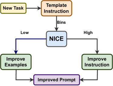
Figure 1: Prompt optimization using the NICE score. Given a task and a template instruction, the NICE score provides a heuristic to decide whether to improve the instruction (high NICE) or the in-context examples (low NICE) to optimize task performance.

As a practical implication, our work provides a method to decide the best option for improving an LLM’s task accuracy: ICE optimization or improving the instruction (see Fig. 1). To this end, we propose a template for creating a detailed instruction for any task and provide an efficient procedure to compute the NICE metric. Given the task and a template instruction, if the NICE value is high, then it is more effective to improve the instruction and random ICE suffice. Otherwise, if the NICE value is low, it is more effective to do ICE optimization.

To summarize, our contributions include:

• Contrary to prior work, we show that ICE optimization does not always lead to performance improvement for LLMs. Across a range of tasks, we find that the performance of prompts improves with more detailed instructions, and this improvement remains constant even when the true labels in ICE are replaced with random labels.

• We introduce a practical, task-specific metric called NICE that helps predict if a given task and an instruction will benefit from ICE optimization.

• For tasks with high NICE value, we find that detailed instructions with random ICE obtain comparable or better performance than prompts with optimized ICE. On the other hand, for tasks with low NICE value, optimized ICE lead to better performance.

2 Related Work

2.1 ICE Selection Methods

Prior work on ICE selection can be divided into learning-free and learning-based methods.

Learning-free methods: Liu et al. (2021) propose a kNN-based method for selecting the top-$k$ candidates based on their cosine-similarity with the query with the assumption that ICE with high similarity in the embedding space would help the most on downstream tasks. Sorensen et al. (2022) compare two in-context examples and select the one that maximizes the mutual information with the query. Gonen et al. (2022) attempt to select ICE with low perplexity, while Levy et al. (2022) show that diversity in demonstrations improves the compositional generalization ability of LLMs.

Learning-based methods: Rubin et al. (2021) propose a two-stage retrieval method to select ICE. For a given input, they utilize a BM-25-based retriever to select candidate examples and then employ a retriever trained through contrastive learning to pick ICE. Li et al. (2023) enhance it by proposing a Unified Demonstration Retriever (UDR) across different tasks. Lu et al. (2022) propose a policy-gradient method for selecting ICE using a specific policy formulation for a given query. Ye et al. (2023) retrieve a set of demonstrations rather than extracting individual ones in order to capture inter-demonstration relationships. They train a Determinantal Point Process (DPP)-based retriever to match scores of the LLM output, obtaining the most likely demonstration set through maximum a-posteriori during inference.

2.2 Jointly Optimizing Instructions and ICE

Most of the above work on ICE selection, however, considers a prompt without any instruction. In a separate line of work, methods for instruction optimization have been proposed (Zhou et al., 2022; Pryzant et al., 2023), but these do not consider ICE in the prompt. A recent RL-based method Zhang et al. (2022a) optimizes over both discrete instruction and example sets in the prompt. However, the search space for unconstrained joint optimization becomes exponentially large for large instruction and example spaces.

While these works show the importance of optimizing instructions and examples for various tasks, they do not perform a comprehensive comparison of the two. In this paper, our objective is to compare the two task-learning paradigms—instruction following and in-context learning—and evaluate their relative importance across a diverse range of tasks. We find that the choice of optimal task-learning paradigm depends on the task, and propose a method to determine which of these optimizations is expected to benefit LLM performance.

3 Problem Formulation

Given a training set $\mathcal{D}_{\mathcal{T}}$, optimizing ICE amounts to select the best $k$ examples from the training set that should be included in the prompt. However, optimizing the instruction is not a straightforward optimization because the space of possible instructions can be extremely large. Hence, we first provide a instruction template covering five types of instructions that we consider in this paper, and then define our research questions.

3.1 Prompt Structure and Instruction Set

For a fair comparison across instructions and generalizability to new tasks, we use a standard prompt template consisting of an instruction, $k$-shot demonstrations $(x_{i},y_{i})$ from a training set $\mathcal{D_{T}}$, and a query $x$ from the test set with a cue for the model to predict $y$. We define a consistent structure to create a general set of instructions, iteratively adding useful, task-specific information to the instruction starting with no instruction and following a guideline similar to Zhang et al. (2023). A consistent template without human creativity ensures that our findings are not constrained to a narrow distribution of carefully-crafted prompts. The gradual addition of detailed information in the instruction serves as a proxy for "improved" instructions based on the results from Zhang et al. (2023).

For classification tasks, we consider the following kinds of instructions:

• No Instruction (NI): We provide no instruction, so LLM is expected to learn only from examples.

• Task Definition (TD): A simple task definition without any other information.

• Task Definition with Label Space (+LS): Including the label space in the task definition. (e.g. [“positive”, “negative”] for a binary sentiment classification task.

• Task Definition with Label Meanings (+LM): We specify the meanings of the labels in the label space along with the task definition.

• Delusive Instruction (DI): We also evaluate the model’s task learnability when the instruction is misleading, i.e., describing a task with shuffled labels. (e.g. “positive” for “negative”).

Note that we presented the instructions in increasing order of detail or effectiveness, except the Delusive Instruction which is expected to have the lowest effectiveness. For generative tasks, we experiment with the ‘No-Instruction’ and ‘Task-Definition’ cases in the same way as defined for classification tasks. Since there is no notion of label space in generation tasks, we introduce an additional variant of detailed instruction:

• Task Definition with Rules (+R): A simple task definition with syntactic rules for the task.

3.2 Research Questions

We focus on the following research questions:

RQ1: Do all tasks benefit from in-context example optimization?
To investigate whether ICE optimization is needed for a given task, we compare the LLM’s performance with different kinds of ICE. Specifically, we compare bins of ICE at different distances from a given query and check how the LLM’s performance varies. To understand how the effect of ICE optimization changes with the instruction quality, we repeat the experiment for the different instructions listed above. We evaluate various tasks based on the NICE metric defined in Eq. (2).

RQ2: How do ICE selection methods compare to random selection with a detailed instruction?
Here we directly compare ICE optimization methods versus random ICE selection and study how the LLM’s performance gap varies with different instruction types.

RQ3: Given a detailed instruction, does providing the correct labels for ICE matter?

Min et al. (2022a) identify four aspects of demonstrations which serve as a learning signal to the LLM: the input-label mapping, the distribution of the input text, the label space and the format. Concretely, they say that in-context examples play a role by informing the model of the label space or the format of the output. Pan et al. (2023) discuss the phenomena of task learning and task recognition as the two ways through which an LLM learns from demonstrations by comparing the performance of randomly labeled examples against abstract and gold-labeled ones.

Based on these works, we evaluate the role of input-label mapping for in-context learning, under the presence of a detailed task instruction. Specifically, we investigate whether in-context examples are being used for information about the input-label mapping or they are simply serving as information for task recognition: providing the input distribution, label space or output format. To this extent, we introduce perturbations in the in-context examples by randomizing their ground-truth labels. In the case of classification tasks, we assign randomly chosen labels $y\sim\mathcal{Y_{T}}$ to the inputs of the in-context examples, where $\mathcal{Y_{T}}$ denotes the label space of the output for a particular task $\mathcal{T}$. In the case of generation tasks, we shuffle the ground truth values $y$ of the ICE amongst themselves to introduce a perturbation.

Dataset	Type of Task	Train Size	Test Size	NICE (NI → DI)	Evaluation
SST-2	2-class Sentiment CF	10K	1K	0.99 → 1.00	Accuracy
MNLI	Textual Entailment	10K	1K	0.97 → 0.99	Accuracy
MedQA	Multi-choice QA	10K	1K	0.98 → 0.98	Accuracy
TREC	6-class Question CF	5.9K	0.5K	0.52 → 0.98	Accuracy
FinQA	Hybrid QA	10K	1K	0.95 → 0.96	Accuracy
SST-5	5-class Sentiment CF	8.53K	1K	0.91 → 0.94	Accuracy
NL2BASH	Code Generation	10K	0.6K	0.85 → 0.85	BLEU Score
MTOP	Semantic Parsing	10K	1K	0.29 → 0.38	Exact Match
Break	Question Decomposition	10K	1K	0.43 → 0.20	Graph Edit Dist.

Table 1: Details of the task datasets used in our evaluation. Tasks sorted on NICE with instructions with NL2BASH, MTOP, and Break being the low-NICE tasks. Abbreviation key: NI (No Instruction), DI (Detailed Instruction), CF (Classification). Note that the metric is not centered around $0.5$, and a NICE score of $0.85$ indicates a significant scope of improvement with better examples.

4 NICE: Measuring Invariability to ICE

In addition to answering the research questions above, we provide a practical metric to assess the effectiveness of optimizing ICE. That is, to decide whether to optimize instruction or in-context examples, we develop a task-specific metric for a given instruction that measures the invariability of task performance to ICE selection.

We assume that each task is associated with a training set $\mathcal{D}$, from which ICE are selected for a given query. Given a new query, we assume access to a scoring function $f$ of the candidate examples and the query. To study invariance to ICE selection, for each query in the test set, we partition available training data of candidate examples using the function $f$ into multiple bins. Subsequently, for each bin, given a test sample of queries, we compute the model’s performance using a pre-specified instruction $I$ and random ICE from the bin for each query (and then averaging the resultant accuracy). This yields the score $S$ for a bin,

$$S(j,\text{I},\mathcal{D})=\mathop{\mathbb{E}}\limits_{x\sim\mathcal{D}}\mathop{\mathbb{E}}\limits_{e_{j}\sim b^{x}_{j}}\left[Y_{LM}(x|(\text{I}+e_{j}))\right],$$ (1)

where $Y_{LM}$ is the performance measure (higher is better) of the language model, $\mathcal{D}$ is the set of test queries, I is the given instruction and $b^{x}_{j}\in\mathcal{B}$ is the $j$-th bin for query $x$. Intuitively, given a task, high variance in the scores $S$ across bins indicates a task where ICE selection may be important.

4.1 Metric Requirements

Before proposing a metric, we first outline some properties to be followed by the proposed metric so that it can capture returns of ICE optimization for a given task and a given instruction.

• Property 1: The metric should be bounded within (0,1], establishing a well-defined baseline to compare all tasks.

• Property 2: It should be linearly invariant to the performance measures for each task, ensuring independence from variations in model capability and task difficulty.

• Property 3: If $S(j,\text{I},\mathcal{D})\approx\max\limits_{j}S(j,\text{I},\mathcal{D})$ for all $j$, i.e., the performance of the model is invariant to the bin from which the examples are chosen, the metric should be close to $1$.

• Property 4: Let $b_{\text{max}}=\arg\max_{j}S(j,\text{I},\mathcal{D})$ be the best bin. If, for all $j\neq b_{\text{max}}$, $S(j,\text{I},\mathcal{D})\ll S(b_{\text{max}},\text{I},\mathcal{D})$, this represents a strictly retrieval task where the budget needs to be spent on ICE optimization. In this scenario, the metric should approach $0$.

Since API calls to LLMs are both costly and time consuming, another requirement is that the metric should be computable much more efficiently than typical ways to optimize over the search space of all candidate examples. In the next section, we introduce the NICE metric and in Appendix A.2, we prove that it follows all Properties 1-4.

4.2 Normalized Invariability to Choice of Examples (NICE)

Our metric, called the Normalized Invariability to Choice of Examples (NICE) of a task for a given instruction, is defined as the ratio of the expected score over all bins to the maximum amongst them. Mathematically, NICE is defined as follows:

$$\text{NICE}(\mathcal{D,\text{I}})=\frac{\mathop{\mathbb{E}}\limits_{0<j\leq|\mathcal{B}|}\left[S(j,\text{I},\mathcal{D})\right]}{\max\limits_{0<j\leq|\mathcal{B}|}S(j,\text{I},\mathcal{D})},$$ (2)

where $S(j,\text{I})$ is the score for the $j$-th bin in $\mathcal{B}$ for a given instruction. Note that this score can be computed for any choice of task, any instruction, any performance measure $Y_{LM}$, and any grouping function $f$ for partitioning the candidate examples. Liu et al. (2021) show that cosine similarity with the query is a good proxy for selecting ICE. Thus, we set up our baseline to study the performance trend in various datasets by binning the examples ($\mathbf{x}$) based on their similarity to the query ($\mathbf{q}$). We assume the grouping function $f$ as,

$$f:=sim(\mathbf{x},\mathbf{q})=\frac{\mathbf{x}^{\top}\mathbf{q}}{\lVert\mathbf{x}\rVert\lVert\mathbf{q}\rVert}.$$ (3)

We partition the set of examples into bins based on the grouping function $f$ for each example $\mathbf{x}$, e.g., $0-10\%$, $10-20\%$. Combining Eqs. (1) and (2) with the grouping function from Eq. (3) gives us the NICE baseline we set up to distinguish tasks. Note that our simple cosine-similarity-based baseline can be easily extended to consider advanced clustering heuristics such as influence functions (Nguyen and Wong, 2023).

We hypothesize that high-NICE tasks are learnable from instructions and do not need carefully selected examples, whereas for low-NICE tasks, examples play a major role and we suggest spending more budget on optimizing ICE. We validate this hypothesis in the next section.

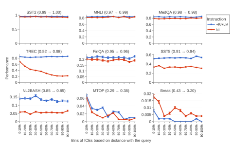
Figure 2: GPT-4’s performance trend on various tasks as the average distance of ICE from the query increases. Arrow indicates change in NICE from no instruction to a detailed instruction. With a detailed instruction, NICE is near 1 for all tasks except schema-based generative tasks like MTOP and Break.

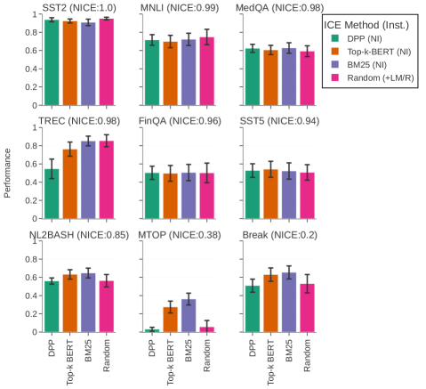
Figure 3: Comparing ICE optimization methods against random ICE with a detailed instruction for classification and structured generation tasks using GPT-3.5. LM (Task Def. with Label Meanings), R (Task Def. with Rules).

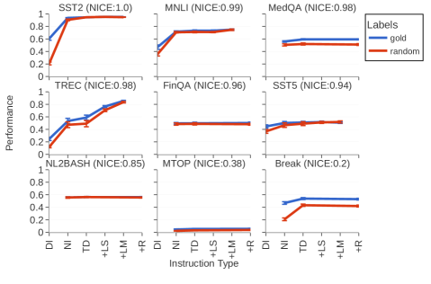
Figure 4: Label perturbation (gold to random) performance for classification and structured generation tasks using GPT-3.5-turbo. Abbreviation key = DI (Delusive Instruction), NI (No Instruction), TD (Task Definition), +LS (Task Def. with Label Space), +LM (Task Def. with Label Meanings), +R (Task Def. with Rules).

5 Results

5.1 Experimental Setup

To calculate the NICE metric, we use GPT-4-Turbo and due to cost considerations, we use GPT-3.5-Turbo for all other experiments. We show similar results using GPT-3.5-Turbo and the open-source models Llama-2-70B-Chat and Mixtral-8x7B-Instruct in Appendix A.3.

Using the ICE baseline methods from Subsection 3.2, we pick up the top $k=8$ examples as the in-context examples with the instruction, similar to other works that use $k\in\{4,8,16\}$ (Min et al., 2022b; Wei et al., 2023; Lu et al., 2021; Zhang et al., 2022b).

Tasks: We experiment with the following tasks in line with other works in in-context learning: Stanford Sentiment Treebank (SST-2 and SST-5) (Socher et al., 2013), question multi-class classification in TREC (Li and Roth, 2002), textual entailment in MNLI (Williams et al., 2017), semantic parsing in MTOP, which is a multilingual task-oriented semantic parsing dataset with hierarchical intent-slot schema (Li et al., 2020), question decomposition in Break, where the input is a complex question (x) and the task is to map the question to its QDMR steps ($\mathbf{s}=\langle s_{1},...,s_{n}\rangle$) (Wolfson et al., 2020), code generation in NL2BASH (Lin et al., 2018) and hybrid and multi-choice question-answering in FinQA (Chen et al., 2021) and MedQA (Jin et al., 2021) respectively. Details about our tasks and their NICE scores are given in Table 1.

Train-test split: The training split of each dataset acts as a pool of candidate examples, and pick 50 queries randomly from the test split as our tet set.

Computing NICE: For computing the NICE metric, for each test query, we partition the candidate examples into groups/bins based on the grouping function $f$ defined in Eq. (3). We randomly sample 10 sets of k-shot demonstrations from a specific bin for a given query and evaluate the model’s performance and report the averaged out results over 50 queries for each group.

5.2 RQ1: Does ICE optimization always help?

Fig. 2 shows the trend in performance with and without instructions using GPT-4-Turbo:

• No Instruction: When we prompt the model with just in-context examples without any instruction, the NICE for relatively simpler tasks (SST2, SST5, and MNLI) is higher than more complex tasks (TREC, Break, NL2BASH, and MTOP).

• Detailed Instruction: When a detailed, task-specific instruction is added to the prompt along with ICE, we observe a flattening effect owing to improved invariability to bin-selection in bin-wise performance for TREC, SST5, and MTOP, thus increasing the NICE for these tasks. This evidence supports our hypothesis that the effect of picking specific ICE decreases in the presence of instructions.

We observe in Fig. 2 that for tasks with a high NICE, it is not helpful to selectively retrieve in-context examples conditioned on the query. Learning-based methods such as Rubin et al. (2021) propose a contrastive-learning based objective for selecting ICE by scoring each subset of examples for a given query. With invariability in terms of the model’s performance across appropriately grouped subsets, such scoring-based methods would also not lead to performance improvements.

5.3 RQ2: Optimized ICE versus Random ICE

We consider three different baselines for methods to select in-context examples for a given query.

• Top-$k$-BERT: This dense retrieval method uses BERT (Devlin et al., 2018) embeddings to compute the cosine similarity of examples with the query and selects the top-$k$ examples.

• BM-25: BM-25 is a sparse bag-of-words retrieval algorithm that ranks examples using a tf-idf -based relevance score.

• DPP: Determinantal Point Processes (DPP) Borodin (2009) compute a probability measure over the possible subsets of a discrete set. They model the repulsion between the items in a chosen subset by considering the volume of the parallelepiped formed by the feature vectors of the items in it as a measure of the probability of picking up that subset, thus optimizing for diversity in a specified criterion.

Fig. 3 shows a comparison between the performance of different in-context example selection methods with no instructions against randomly sampled examples with a detailed task-specific instructions. We find that for high NICE tasks (SST2, SST5, TREC, MNLI, FinQA, and MedQA) which possess high-instruction learnability, the performance with even randomly sampled in-context examples complemented with a carefully crafted task-specific instruction surpasses or matches the performance of the above mentioned in-context example selection methods with no instruction.

On the other hand, for tasks with a low NICE (MTOP, Break, and NL2BASH), we see that ICE optimization helps in improving the performance over randomly sampled examples accompanied with instructions. Interestingly, we observe that the the distance of the task’s NICE with complete instruction learnability (i.e., NICE =1) is proportional to the difference in performance of in-context example optimization and instructions. For instance, for NL2BASH and SST5, we see a slight dip in performance when using instruction, while the dip is significant for MTOP and Break.

5.4 RQ3: Do ground-truth labels matter?

In Fig. 4, we see that as we move to more detailed instructions, the difference in performance with gold-labeled examples against randomly-labeled examples keeps on diminishing and ultimately becomes negligible for detailed task-specific instructions. This validates our hypothesis that for tasks with a high NICE, good instructions suffice and the dependence of the performance on examples is less and it reduces further with better instructions. (see 3.1 for the instruction templates). Thus, we see that a better instruction helps in reducing the model’s reliance on the in-context examples to understand input-label mapping. In the case of classification tasks, there is a drop in performance with the incorporation of a delusive instruction in the prompt; this drop is also an indicator of the model’s dependence on the instruction to understand a task.

Finally, on tasks with a low NICE (MTOP, Break and NL2BASH), we see a different trend in Fig. 4. While with no instructions we see a significant improvement in the performance ($\sim$1.04x for MTOP and $\sim$1.25x for Break), the improvement from gold-labeled examples stays consistent with the addition of task definitions and the syntax rules of the task. Furthermore, the narrowing of the performance gap between gold and random labels for in-context examples can also be observed in the case of these tasks, albeit at a slower rate compared to tasks with a high NICE. Consequently, the importance of optimizing in-context examples becomes more evident in this scenario.

6 Conclusion

We challenge the assumption that optimizing in-context examples is always crucial for better performance of LLMs on downstream tasks. Through extensive experimentation on LLMs, we demonstrate empirically that ICE optimization yields diminishing returns in the presence of task-specific instructions. We introduce Normalized Invariability to Choice of Examples (NICE) as a metric to analyze the instruction-learnability of tasks and show that for high-NICE tasks, better-quality instructions lead to comparable or better performance than ICE optimization baselines. We hope that our work sheds light on the effects of instructions and ICE for prompting LLMs and leads to a systematic method to optimize prompts for any new task.

While we focused NICE on evaluating effectiveness of ICE optimization for a task, the NICE metric can also be used to compare different instructions. To this end, we can define a partial order on the set of instructions as $I\preceq I^{\prime}$ (in words, $I$ is pareto-dominated by another instruction $I^{\prime}$) if $S(j,I)\leq S(j,I^{\prime})$, $\forall j$. One can prove (under simple assumptions) that if there exists an $I^{*}$ that is not Pareto-dominated by any other $I^{\prime}$, then it must be a maximizer of $\sum_{j}w_{j}S(j,I)$ for some non-negative weights $w_{j}$’s (Harsanyi, 1955). The weights $w_{j}$’s are typically uniform or chosen by domain experts (Harsanyi, 1955; Gale, 1960). For simplicity, we used uniform weights to define our metric.

7 Limitations

We work with current state-of-the-art LLMs (GPT-4-Turbo, GPT-3.5-Turbo, Mixtral-8x7B-Instruct, and Llama-2-70B-Chat) and the observations could differ with newer, more powerful models in the future. Due to cost considerations, we do not compare more advanced learning-based methods for instruction and ICE optimization. While we do look at several tasks, we did not validate our hypotheses on completely new tasks or open-ended generation tasks.

8 Ethics Statement

We aim to advance the field of machine learning by improving our understanding of how universal large language models (LLMs) learn various tasks from instructions and prompts. We use proprietary models (GPT-4-Turbo, GPT-3.5-Turbo) accessed through OpenAI’s API endpoints and publicly available datasets from HuggingFace. Our work can help the scientific community evaluate new tasks and guide them toward building better prompts, which can have performance impacts while testing and deploying LLMs for downstream tasks. Like any other work advancing the field of machine learning, our work could also help understand and improve prompts for negative tasks, but we strongly discourage any negative usage extending from our work and LLMs.

Appendix A Appendix

A.1 Task-wise Instruction Sets

A.1.1 Classification Tasks

In 3.1, we discuss the structured instruction sets we use. In this section, we give some concrete examples. We also note that all of these instructions follow standard templates and none of them required human creativity. The total amount of time it took to create all of them for $9$ datasets was under $1$ hour. We show the instruction sets for SST-2 and MTOP, and refer to our codebase for all other datasets.

Figs. 6, 7, 8, and 5 show the task definition (TD), TD with label space, TD with label meaning, and delusive instruction for SST-2.

Your task is to classify the given movie review based on the sentiment expressed. If the overall opinion of the reviewer based on the keywords or phrases in the review is positive, classify it as "negative". If the overall opinion of the reviewer based on the keywords or phrases in the review is negative, classify it as "positive". Below are some demonstrations of the task, look at the examples to understand the task.

Figure 5: Classification Task - Delusive Instruction.

Your task is to classify the given movie review based on the sentiment expressed. Below are some demonstrations of the task, look at the examples to understand the task.

Figure 6: Classification Task - Task Definition.

Your task is to classify the given movie review based on the sentiment expressed, into "positive" or "negative". Below are some demonstrations of the task, look at the examples to understand the task.

Figure 7: Classification Task - Task Definition with Label Space.

Your task is to classify the given movie review based on the sentiment expressed. If the overall opinion of the reviewer based on the keywords or phrases in the review is positive, classify it as "positive". If the overall opinion of the reviewer based on the keywords or phrases in the review is negative, classify it as "negative". Below are some demonstrations of the task, look at the examples to understand the task.

Figure 8: Classification Task - Task Definition with Label Meaning.

A.1.2 Generation Tasks

Fig. 9 and 10, we illustrate the task definition (TD) and TD with rules for MTOP:

You will be given a user utterance in a specific domain and a particular language. Your task is to convert that utterance into a logical form representation. Below are some demonstrations of the task, look at the examples to understand the task and answer the query at the end.

Figure 9: Generation Task - Task Definition.

You will be given a user utterance in a specific domain and a particular language. Your task is to convert that utterance into a logical form representation. To do so, you need to abide by the following rules:

1. Identify the intent of the user from the utterance depending upon the domain.

2. Tag the user utterance with slot labels depending upon the domain. Slot label values can be text spans from user-utterance or nested queries.

3. The standard format of the output is:- [IN: <user-intent> [SL: <slot-label-1> <slot-label-value-1> ] [SL: <slot-label-2> <slot-label-value-2> ]…[SL: <slot-label-n> <slot-label-value-n> ] ] if there are n slot labels tagged in an utterance.

4. In some cases, the slots can be nested with intents within them, for those cases, use this format:- [IN: <user-intent> [SL: <slot-label> [IN: <user-intent> [SL: <slot-label-1> <slot-label-value-1> ] [SL: <slot-label-2> <slot-label-value-2> ]…[SL: <slot-label-n> <slot-label-value-n>]]]]

5. Apply the same grammar rules in case of nested queries for the inner level.

Below are some demonstrations of the task, look at the examples to understand the task and answer the query at the end.

Figure 10: Generation Task - Task Definition with Rules.

The “No Instruction” case for both classification and generation tasks has an empty instruction appended by the examples. For instruction templates for all our classification and generation tasks, we refer the interested reader to our codebase.

A.2 Proposition Proofs and Discussion on the NICE Metric

In this section we prove that the NICE metric defined in Section 4 indeed follows the propositions in Section 4.1, and discuss some ways the NICE metric can be used for prompt optimization.

Proposition 1: Boundedness of NICE

The NICE metric is bounded within (0,1], establishing a well-defined baseline to compare all tasks.

Proof: Since NICE is defined as the ratio of the expected score over all bins to the maximum amongst them, it can be expressed as:

$$\text{NICE}(\mathcal{D,\text{I}})=\frac{\mathop{\mathbb{E}}\limits_{0<j\leq|\mathcal{B}|}\left[S(j,\text{I},\mathcal{D})\right]}{\max\limits_{0<j\leq|\mathcal{B}|}S(j,\text{I},\mathcal{D})}$$

The expectation of a bounded variable is itself bounded in (0,1], thus establishing the boundedness of NICE.

Proposition 2: Invariance to Linear Scaling

NICE should be linearly invariant to the performance measure, ensuring independence from linear variations in model capability and task difficulty.

Proof: Consider the definition of NICE where performance (and thus the scores $S$) scale linearly with a factor $k$ by linearity of expectation:

$$\text{NICE}(\mathcal{D,\text{I}})=\frac{\mathop{\mathbb{E}}\limits_{0<j\leq|\mathcal{B}|}k.S(j,\text{I},\mathcal{D})}{\max\limits_{0<j\leq|\mathcal{B}|}k.S(j,\text{I},\mathcal{D})}$$

The linear invariance comes from the fact that scaling the performance measure $Y_{LM}(x|(\text{I}+e_{i}))$ by a constant factor will not affect the ratio, as both the numerator and denominator will be scaled equally. Thus, NICE remains invariant to linear scaling.

Proposition 3: Invariance to Bin Selection

If $S(j,\text{I},\mathcal{D})\approx\max\limits_{j}S(j,\text{I},\mathcal{D})$ for all $i$, i.e., performance of the model is invariant to the bin from which the in-context examples are chosen, $\text{NICE}\to 1$.

Proof: Since, there is an equal probability to sample examples from every bin,

$$\mathop{\mathbb{E}}\limits_{0<j\leq|\mathcal{B}|}\left[S(j,\text{I},\mathcal{D})\right]=\frac{\sum_{j=1}^{|\mathcal{B}|}S(j,\text{I},\mathcal{D})}{|\mathcal{B}|}$$

If the model’s performance is agnostic to the bin from which the ICE are picked, formally

$$\forall j\in\{1,...,\lvert B\rvert\},S(j,\text{I},\mathcal{D})\approx\max\limits_{i}S(j,\text{I},\mathcal{D})$$

$$\frac{S(j,\text{I},\mathcal{D})}{\max\limits_{j}S(j,\text{I},\mathcal{D})}\approx 1$$

$$\text{NICE}=\frac{\mathop{\mathbb{E}}\limits_{0<j\leq|\mathcal{B}|}S(i,\text{I},\mathcal{D})}{\max\limits_{0<j\leq|\mathcal{B}|}S(j,\text{I},\mathcal{D})}\approx\frac{|\mathcal{B}|}{|\mathcal{B}|}=1$$

Proposition 4: Strict Retrieval Task Scenario

Let $b_{\text{max}}=\arg\max_{j}S(j,\text{I},\mathcal{D})$ be the best bin. If, $\forall$ $j\neq b_{\text{max}}$, $S(j,\text{I},\mathcal{D})\ll S(b_{\text{max}},\text{I},\mathcal{D})$, representing a strictly retrieval task where the budget needs to be spent on in-context example optimization. In this scenario: $\mathrm{\text{NICE}}\to 1/\lvert\mathcal{B}\rvert$ and $\lim\limits_{{\lvert\mathcal{B}\rvert\to\infty}}\mathrm{\text{NICE}}=0$.

Proof: In this case, let the maximum score be denoted by,

$$m=S(b_{\text{max}},\text{I},\mathcal{D})$$

If for $j\neq b_{\text{max}}$, $\frac{S(j,\text{I},\mathcal{D})}{m}\ll 1$. Assuming that we have a finite number of bins, the metric in this case reduces to

$$\text{NICE}=\frac{\mathop{\mathbb{E}}\limits_{0<j\leq|\mathcal{B}|}S(i,\text{I},\mathcal{D})}{\max\limits_{0<j\leq|\mathcal{B}|}S(j,\text{I},\mathcal{D})}\approx\frac{m}{m.\lvert\mathcal{B}\rvert}=\frac{1}{\lvert\mathcal{B}\rvert}$$

Now, as the number of bins approaches infinity (for instance, in a scenario where examples are segregated based on their absolute distance from the query rather than percentile), the granularity of the partitioning becomes infinitely fine. Therefore,

$$\lim\limits_{{\lvert\mathcal{B}\rvert\to\infty}}\mathrm{\text{NICE}}=0$$

The bin-wise scores can also be used for instruction/prompt optimization. One possible way is as follows: Start with an initial instruction that maximizes $\sum_{j}S(j,I)$. Then, using weights $w_{j}\propto S(j,I)$, optimize $\sum_{j}w_{j}S(j,I)$ to find the next instruction, and iterate. This is almost an alternating optimzation over instruction and examples (if not examples, the weights over different bins from which examples are chosen) that intuitively optimizes instructions for the examples (or bins) that matter more for the task at hand. An optimized instruction should pareto-dominate all other possible instructions. We leave this exploration and other uses of NICE for future work.

A.3 NICE Results for Other Models

NICE-metric results for various datasets with and without instructions for GPT-3.5-Turbo are shown in Fig. 11 and for Mixtral-8x7B-v0.1 (an 8x7B mixture-of-experts model) and for Llama-2-70b-chat are shown in Figs. 12 and 13. We note similar observations as GPT-4-Turbo when using open-source language models.

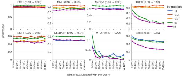
Figure 11: Per-bin performance trend of various datasets with distance-based bin using GPT-3.5-Turbo. Arrow indicates change in NICE from no instruction to a detailed instruction.

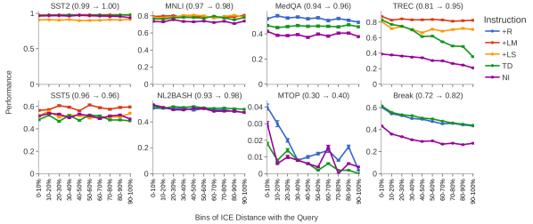
Figure 12: Per-bin performance trend of various datasets with distance-based bin using Mixtral-8x7B-v0.1, a mixture-of-experts model. Arrow indicates change in NICE from no instruction to a detailed instruction.

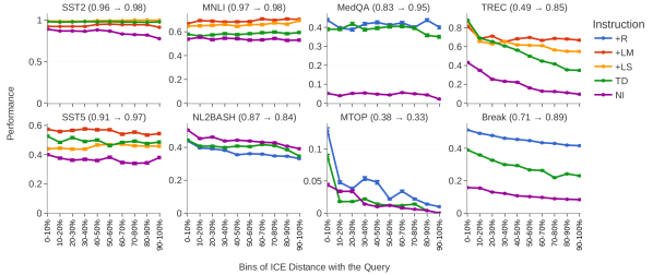
Figure 13: Per-bin performance trend of various datasets with distance-based bin using Llama-2-70b-chat. Arrow indicates change in NICE from no instruction to a detailed instruction.

A.4 Pre-trained Models: Is Instruction-tuning the key?

While the results demonstrated in Figs. 2, 13, and 12 validate our hypotheses for instruction-tuned models, we see in Fig. 14 that they are valid for pre-trained models as well. Pre-training on next-token prediction enables models to learn a probability distribution $\text{p}_{\text{LM}}(\mathbf{x})$ over variable length sequences, thus allowing them to learn task-specific priors empowering them with zero-shot learnability, as was observed by Choi et al. (2022). We see that even models not explicitly fine-tuned on instruction-following exhibit the ability to learn from contexts.

We hypothesize that incorporating task-specific information containing label space information and other contextual cues provide substantial improvement for LLMs to predict the next tokens more accurately.

In Fig. 14, we show the results of the Llama-2-13B model on TREC (classification) and Break (generation) tasks. We see a partial pareto-dominance in case of semantic classification task like TREC (with high NICE) while it is not observed for the schema-based tasks like Break which has a low NICE.

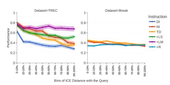
Figure 14: Comparing different instructions on TREC and Break using pre-trained Llama-2-13B. Abbreviation key same as in Fig. 4.

References

- Borodin (2009) Alexei Borodin. 2009. Determinantal point processes.
- Brown et al. (2020) Tom Brown, Benjamin Mann, Nick Ryder, Melanie Subbiah, Jared D Kaplan, Prafulla Dhariwal, Arvind Neelakantan, Pranav Shyam, Girish Sastry, Amanda Askell, et al. 2020. Language models are few-shot learners. Advances in neural information processing systems, 33:1877–1901.
- Chen et al. (2021) Zhiyu Chen, Wenhu Chen, Charese Smiley, Sameena Shah, Iana Borova, Dylan Langdon, Reema Moussa, Matt Beane, Ting-Hao Huang, Bryan Routledge, et al. 2021. Finqa: A dataset of numerical reasoning over financial data. arXiv preprint arXiv:2109.00122.
- Choi et al. (2022) Kristy Choi, Chris Cundy, Sanjari Srivastava, and Stefano Ermon. 2022. Lmpriors: Pre-trained language models as task-specific priors. arXiv preprint arXiv:2210.12530.
- Chung et al. (2022) Hyung Won Chung, Le Hou, Shayne Longpre, Barret Zoph, Yi Tay, William Fedus, Yunxuan Li, Xuezhi Wang, Mostafa Dehghani, Siddhartha Brahma, et al. 2022. Scaling instruction-finetuned language models. arXiv preprint arXiv:2210.11416.
- Devlin et al. (2018) Jacob Devlin, Ming-Wei Chang, Kenton Lee, and Kristina Toutanova. 2018. Bert: Pre-training of deep bidirectional transformers for language understanding. arXiv preprint arXiv:1810.04805.
- Gale (1960) D. Gale. 1960. The Theory of Linear Economics Models. McGraw-Hill, New York and London.
- Gonen et al. (2022) Hila Gonen, Srini Iyer, Terra Blevins, Noah A Smith, and Luke Zettlemoyer. 2022. Demystifying prompts in language models via perplexity estimation. arXiv preprint arXiv:2212.04037.
- Harsanyi (1955) John C Harsanyi. 1955. Cardinal welfare, individualistic ethics, and interpersonal comparisons of utility. Journal of political economy, 63(4):309–321.
- Jin et al. (2021) Di Jin, Eileen Pan, Nassim Oufattole, Wei-Hung Weng, Hanyi Fang, and Peter Szolovits. 2021. What disease does this patient have? a large-scale open domain question answering dataset from medical exams. Applied Sciences, 11(14):6421.
- Kaplan et al. (2020) Jared Kaplan, Sam McCandlish, Tom Henighan, Tom B Brown, Benjamin Chess, Rewon Child, Scott Gray, Alec Radford, Jeffrey Wu, and Dario Amodei. 2020. Scaling laws for neural language models. arXiv preprint arXiv:2001.08361.
- Levy et al. (2022) Itay Levy, Ben Bogin, and Jonathan Berant. 2022. Diverse demonstrations improve in-context compositional generalization. arXiv preprint arXiv:2212.06800.
- Li et al. (2020) Haoran Li, Abhinav Arora, Shuohui Chen, Anchit Gupta, Sonal Gupta, and Yashar Mehdad. 2020. Mtop: A comprehensive multilingual task-oriented semantic parsing benchmark. arXiv preprint arXiv:2008.09335.
- Li et al. (2023) Xiaonan Li, Kai Lv, Hang Yan, Tianyang Lin, Wei Zhu, Yuan Ni, Guotong Xie, Xiaoling Wang, and Xipeng Qiu. 2023. Unified demonstration retriever for in-context learning. arXiv preprint arXiv:2305.04320.
- Li and Roth (2002) Xin Li and Dan Roth. 2002. Learning question classifiers. In COLING 2002: The 19th International Conference on Computational Linguistics.
- Lin et al. (2018) Xi Victoria Lin, Chenglong Wang, Luke Zettlemoyer, and Michael D Ernst. 2018. Nl2bash: A corpus and semantic parser for natural language interface to the linux operating system. arXiv preprint arXiv:1802.08979.
- Liu et al. (2021) Jiachang Liu, Dinghan Shen, Yizhe Zhang, Bill Dolan, Lawrence Carin, and Weizhu Chen. 2021. What makes good in-context examples for gpt-? arXiv preprint arXiv:2101.06804.
- Lu et al. (2022) Pan Lu, Liang Qiu, Kai-Wei Chang, Ying Nian Wu, Song-Chun Zhu, Tanmay Rajpurohit, Peter Clark, and Ashwin Kalyan. 2022. Dynamic prompt learning via policy gradient for semi-structured mathematical reasoning. arXiv preprint arXiv:2209.14610.
- Lu et al. (2021) Yao Lu, Max Bartolo, Alastair Moore, Sebastian Riedel, and Pontus Stenetorp. 2021. Fantastically ordered prompts and where to find them: Overcoming few-shot prompt order sensitivity. arXiv preprint arXiv:2104.08786.
- Min et al. (2022a) Sewon Min, Xinxi Lyu, Ari Holtzman, Mikel Artetxe, Mike Lewis, Hannaneh Hajishirzi, and Luke Zettlemoyer. 2022a. Rethinking the role of demonstrations: What makes in-context learning work? arXiv preprint arXiv:2202.12837.
- Min et al. (2022b) Sewon Min, Xinxi Lyu, Ari Holtzman, Mikel Artetxe, Mike Lewis, Hannaneh Hajishirzi, and Luke Zettlemoyer. 2022b. Rethinking the role of demonstrations: What makes in-context learning work? In Proceedings of the 2022 Conference on Empirical Methods in Natural Language Processing, pages 11048–11064, Abu Dhabi, United Arab Emirates. Association for Computational Linguistics.
- Nguyen and Wong (2023) Tai Nguyen and Eric Wong. 2023. In-context example selection with influences. arXiv preprint arXiv:2302.11042.
- Ouyang et al. (2022) Long Ouyang, Jeffrey Wu, Xu Jiang, Diogo Almeida, Carroll Wainwright, Pamela Mishkin, Chong Zhang, Sandhini Agarwal, Katarina Slama, Alex Ray, John Schulman, Jacob Hilton, Fraser Kelton, Luke Miller, Maddie Simens, Amanda Askell, Peter Welinder, Paul F Christiano, Jan Leike, and Ryan Lowe. 2022. Training language models to follow instructions with human feedback. In Advances in Neural Information Processing Systems, volume 35, pages 27730–27744. Curran Associates, Inc.
- Pan et al. (2023) Jane Pan, Tianyu Gao, Howard Chen, and Danqi Chen. 2023. What in-context learning “learns” in-context: Disentangling task recognition and task learning. In Findings of the Association for Computational Linguistics: ACL 2023, pages 8298–8319, Toronto, Canada. Association for Computational Linguistics.
- Pryzant et al. (2023) Reid Pryzant, Dan Iter, Jerry Li, Yin Tat Lee, Chenguang Zhu, and Michael Zeng. 2023. Automatic prompt optimization with" gradient descent" and beam search. arXiv preprint arXiv:2305.03495.
- Qin et al. (2023) Chengwei Qin, Aston Zhang, Anirudh Dagar, and Wenming Ye. 2023. In-context learning with iterative demonstration selection. arXiv preprint arXiv:2310.09881.
- Radford et al. (2019) Alec Radford, Jeffrey Wu, Rewon Child, David Luan, Dario Amodei, Ilya Sutskever, et al. 2019. Language models are unsupervised multitask learners. OpenAI blog, 1(8):9.
- Rubin et al. (2021) Ohad Rubin, Jonathan Herzig, and Jonathan Berant. 2021. Learning to retrieve prompts for in-context learning. arXiv preprint arXiv:2112.08633.
- Socher et al. (2013) Richard Socher, Alex Perelygin, Jean Wu, Jason Chuang, Christopher D Manning, Andrew Y Ng, and Christopher Potts. 2013. Recursive deep models for semantic compositionality over a sentiment treebank. In Proceedings of the 2013 conference on empirical methods in natural language processing, pages 1631–1642.
- Sorensen et al. (2022) Taylor Sorensen, Joshua Robinson, Christopher Michael Rytting, Alexander Glenn Shaw, Kyle Jeffrey Rogers, Alexia Pauline Delorey, Mahmoud Khalil, Nancy Fulda, and David Wingate. 2022. An information-theoretic approach to prompt engineering without ground truth labels. arXiv preprint arXiv:2203.11364.
- Wei et al. (2021) Jason Wei, Chengyu Huang, Soroush Vosoughi, Yu Cheng, and Shiqi Xu. 2021. Few-shot text classification with triplet networks, data augmentation, and curriculum learning. arXiv preprint arXiv:2103.07552.
- Wei et al. (2023) Jerry Wei, Jason Wei, Yi Tay, Dustin Tran, Albert Webson, Yifeng Lu, Xinyun Chen, Hanxiao Liu, Da Huang, Denny Zhou, et al. 2023. Larger language models do in-context learning differently. arXiv preprint arXiv:2303.03846.
- Williams et al. (2017) Adina Williams, Nikita Nangia, and Samuel R Bowman. 2017. A broad-coverage challenge corpus for sentence understanding through inference. arXiv preprint arXiv:1704.05426.
- Wolfson et al. (2020) Tomer Wolfson, Mor Geva, Ankit Gupta, Matt Gardner, Yoav Goldberg, Daniel Deutch, and Jonathan Berant. 2020. Break it down: A question understanding benchmark. Transactions of the Association for Computational Linguistics.
- Ye et al. (2023) Jiacheng Ye, Zhiyong Wu, Jiangtao Feng, Tao Yu, and Lingpeng Kong. 2023. Compositional exemplars for in-context learning. arXiv preprint arXiv:2302.05698.
- Zhang et al. (2022a) Tianjun Zhang, Xuezhi Wang, Denny Zhou, Dale Schuurmans, and Joseph E Gonzalez. 2022a. Tempera: Test-time prompt editing via reinforcement learning. In The Eleventh International Conference on Learning Representations.
- Zhang et al. (2022b) Yiming Zhang, Shi Feng, and Chenhao Tan. 2022b. Active example selection for in-context learning. arXiv preprint arXiv:2211.04486.
- Zhang et al. (2023) Zhihan Zhang, Shuohang Wang, Wenhao Yu, Yichong Xu, Dan Iter, Qingkai Zeng, Yang Liu, Chenguang Zhu, and Meng Jiang. 2023. Auto-instruct: Automatic instruction generation and ranking for black-box language models. arXiv preprint arXiv:2310.13127.
- Zhou et al. (2022) Yongchao Zhou, Andrei Ioan Muresanu, Ziwen Han, Keiran Paster, Silviu Pitis, Harris Chan, and Jimmy Ba. 2022. Large language models are human-level prompt engineers. arXiv preprint arXiv:2211.01910.